Originally published as: 

 

 

 

 

 

 

 

 

Saynisch, J., Bergmann, I., Thomas, M. (2015): Assimilation of GRACE‐derived oceanic mass 

distributions with a global ocean circulation model. ‐ Journal of Geodesy, 89, 2, pp. 121—139. 

 

DOI: http://doi.org/10.1007/s00190‐014‐0766‐0 

Assimilating GRACE derived oceanic mass distributionswith a global ocean circulation model

J. Saynischa,∗, I. Bergmann-Wolfa, M. Thomasa,b

aHelmholtz Centre Potsdam, GFZ German Research Centre for Geosciences, Earth System Modelling,Potsdam, Germany

bFreie Universität Berlin Department of Earth Sciences, Institute of Meteorology,Berlin, Germany

Abstract

To study the sub-seasonal distribution and generation of ocean mass anomalies, GravityRecovery and Climate Experiment (GRACE) observations of daily and monthly reso-lution are assimilated into a global ocean circulation model with an ensemble basedKalman-Filter technique. The satellite gravimetry observations are processed to be-come time-variable fields of ocean mass distribution. Error budgets for the observa-tions and the ocean model’s initial state are estimated which contain the full covari-ance information. The consistency of the presented approach is demonstrated by in-creased agreement between GRACE observations and the ocean model. Furthermore,the simulations are compared with independent observations from 54 bottom pressurerecorders. The assimilation improves the agreement to high-latitude recorders by upto 2 hPa. The improvements are caused by assimilation induced changes in the atmo-spheric wind forcing, i.e., quantities not directly observed by GRACE. Finally, the useof the developed Kalman-Filter approach as a destriping-filter to remove artificial noisecontaminating the GRACE observations is presented.

Keywords: Data assimilation, GRACE satellite gravimetry, Time variant ocean massdistribution, GRACE error estimation, Correction of atmospheric forcing

1. Introduction

In the field of oceanography, the problem of satellite observations often lies inthe close entanglement of volume, mass and temperature on the one hand and mass,pressure and velocity of water parcels on the other hand. Other than altimetry whichmeasures sea level changes that may originate in salinity, temperature, ocean dynamicsor mass changes, satellite gravimetry measures mass anomalies alone.

From March 2002 on, the GRACE satellites have measured the gravity field of theEarth with unprecedented precision. To synthesize fields of mass anomalies from theGRACE spherical harmonic (Stokes) coefficients, additional post processing is neces-sary, e.g., to reduce the noise in the higher-degree coefficients which results in the wellknown stripes in the GRACE solutions. In the first years of the GRACE mission, lowpass filtering with an isotropic Gaussian filter as described by Wahr et al. (1998) was thestandard procedure. Since then, improvements have been made with the de-correlation

∗Corresponding authorEmail address: saynisch@gfz-potsdam.de (J. Saynisch)

October 29, 2014

method by Swenson and Wahr (2006) and with anisotropic filter designs (e.g., Werthet al., 2009). For smaller regions, the accuracy of these filter methods is insufficient andso called re-parameterization methods were introduced. Information of the spatial andtemporal structure of the observed region is used to improve the mass anomaly fieldsfrom GRACE by using least squares (e.g., Sasgen et al., 2010; Schrama and Wouters,2011). Recently, a GRACE product is released which uses a Kalman-Filter approachand increases the temporal resolution to daily values (Kurtenbach et al., 2012).

Oceanographic GRACE studies deal with the estimation of mass trends (e.g., Quinnand Ponte, 2010), the steric and non-steric contributions to interannual and seasonalsea level variability (e.g., Willis et al., 2008) and the derivation of the mean dynamictopography (e.g., Vianna et al., 2007). Recently, the focus shifted from trend and meanfield estimation to higher frequencies (e.g., Bonin and Chambers, 2011; Quinn andPonte, 2011). These studies note high discrepancies between modeled and observedocean bottom pressure at monthly and sub-monthly periods and recommend to studyand minimize these discrepancies by data assimilation techniques.

The assimilation of geodetic observations is frequently applied in oceanography(e.g., Wenzel and Schröter, 2007; Saynisch et al., 2011b). For gravimetry data, manymodel-to-observation comparisons exist (e.g., Chambers, 2006; Dobslaw and Thomas,2007) but the assimilation of GRACE observations is a newer field of research. Köhlet al. (2012) use an adjoint assimilation method to integrate monthly gravity field data,in combination with other oceanographic observations, in a global ocean circulationmodel. They found that ocean bottom pressure is partly complementary to combina-tions of other oceanographic data sets which include altimetry but the authors note thatin the assimilation context these data sets have larger prior errors. Furthermore, thesecombinations fail in certain regions, e.g., under the sea-ice, are restricted to the upperocean, have a low sampling interval or a low spatial resolution. Our study takes a sim-ilar approach as Köhl et al. (2012) but because of the mentioned problems, focuses onthe information contained in the GRACE measurements alone. The goal of our paperis first to understand the gain to expect from GRACE assimilation in the oceanic con-text and to identify connected problems, sensitivities, physical mechanism, error bud-gets and possible improvements by using the complementary information containedin GRACE without the superposition of error budgets and assumptions from differentobservation types. Consequently, to be entirely consistent, the observation error is es-timated from GRACE data alone and the success of our assimilation is evaluated bycomparisons with direct measurements of ocean mass, i.e, measured by bottom pres-sure recorders. Furthermore, since GRACE data contains significant physical signalsbelow the monthly resolution (Bonin and Chambers, 2011; Kurtenbach et al., 2012;Quinn and Ponte, 2012; Bergmann and Dobslaw, 2012), our study extends the assim-ilation of Köhl et al. (2012) to high-frequency mass variability by using the GRACEobservations of Kurtenbach et al. (2012) which have daily resolution. Instead of anadjoint method, our study applies an ensemble based Kalman-Filter assimilation tech-nique and in contrast to the globally uniform observation error of 1 hPa used in Köhlet al. (2012), a globally varying observation error with full covariance information isincorporated. Despite all aforementioned progress in the processing of GRACE mea-surements, the mass anomalies of different GRACE centers show still significant dif-ferences (Quinn and Ponte, 2008; Sakumura et al., 2014). Because in some regionsthese differences are larger than the distributed formal errors, we use these differencesto estimate the GRACE observation error budget.

The findings of these more fundamental assimilation experiments can be utilizedafterwards for a beneficial assimilation of combinations of oceanographic observations

2

or for the design and motivation of future satellite gravimetry missions.The experiment’s setup is described in Sect. 2. The description includes the ocean

model (Sec. 2.1), the incorporated gravimetry data and its processing (Sec. 2.2), theassimilation method (Sec. 2.3) and the estimation of the incorporated error budgets(Sec. 2.4). In Sect. 3 the results of the GRACE assimilation are presented and dis-cussed. We summarize the obtained results in Sect. 4.

2. Methods and Data

2.1. Ocean model

The Ocean Model for Circulation and Tides (OMCT, Thomas et al., 2001) is usedin this study. Despite the model’s name, tides are switched off to be consistent withthe assimilated GRACE observations (see Sec. 2.2). The applied OMCT version hasa resolution of 1.875 degrees in the horizontal and 13 layers in the vertical direc-tion. This resolution is sufficient, given the fact that the spatial resolution of the as-similated GRACE data is limited by spherical harmonic degree 40, i.e., 1000 km onthe Earth’s surface. Furthermore, Bingham and Hughes (2008) suggest that oceanbottom pressure differences between eddy permitting and coarser resolution oceanmodels are in general small. Quinn and Ponte (2012) show that on sub-seasonaltimescales and for observed variability of some hundred kilometer extent, the ocean isbarotropic. The OMCT’s temporal resolution of 30 minutes is sufficient to assimilatethe daily GRACE observations. The model is forced by 6-hourly ERA-Interim prod-ucts (wind-stress, freshwater-flux, heat-flux) from the European Centre for Medium-Range Weather Forecasts (ECMWF, Uppala et al., 2008) and river runoff from theLand Surface Discharge Model (LSDM, Dill, 2008). The OMCT conserves mass andthe correction of artificial mass change due to the Boussinesq-Approximation followsGreatbatch (1994). In this configuration, the OMCT is well suited for mass relatedstudies in general (Dobslaw and Thomas, 2007), for the modelling of short term oceanbottom pressure variability in particular (Bergmann and Dobslaw, 2012) and is in usefor the GRACE de-aliasing (Flechtner, 2007).

Two different simulations are generated with this model setup. First, the referencesimulation consists of the OMCT’s reaction to the ECMWF forcing and is similar to thesimulation which is used for the GRACE AOD1B-RL04 de-aliasing product (Flecht-ner, 2007). Second, the assimilation simulation consists of the OMCT coupled to anensemble Kalman-Filter (see Sec. 2.3) with the constraint to reproduce observation-based daily ocean bottom pressure fields from GRACE (see Sec. 2.2).

2.2. Gravimetry observations

In this study, daily GRACE solutions from the Institute of Theoretical Geodesy(ITG) of the University of Bonn are assimilated. The ITG-GRACE solutions use aKalman smoother approach to estimate daily gravity fields (Kurtenbach et al., 2012).The Stokes coefficients of ITG-GRACE are provided up to degree N=40. The observa-tions are cut to a time window from January 2003 to August 2009. For the estimationof changes in ocean bottom pressure, non-tidal mass effects of atmosphere and ocean(i.e., the GAC product) are added back. Additionally, the degree 1 term is included asa mean annual sinusoid determined from Satellite Laser Ranging and DORIS obser-vations (Eanes, 2000). Following Wahr et al. (1998), spectral leakage of continentalsignals is minimized by applying a Gaussian filtering with a half-width radius of 300

3

km. Fields of ocean bottom pressure changes are estimated from the Stokes coefficients∆Clm and ∆Slm according to Wahr et al. (1998):

∆pbot(ϕ,λ, t) =aE gρE

3

N

∑l=1

l

∑m=0

2l +11+ kl

Plm sin(ϕ)

·(∆Clm cos(mλ)+∆Slm sin(mλ)),

where aE is the semi-major axis of the reference ellipsoid, ρE the Earth’s meandensity, g the mean gravitational acceleration, kl the load Love numbers of degreel, Plm the normalized associated Legendre functions of degree l and order m, ϕ thegeographical latitude and λ the geographical longitude. The geographical positions areidentical to the grid points of the ocean model used for the assimilation.

In addition, one year (2004) of monthly GRACE data from the Deutsches GeoFor-schungsZentrum (GFZ) are assimilated. The GFZ-data is described in Sec. 2.4 and isassimilated to demonstrate certain properties of our Kalman-Filter approach.

2.3. Assimilation setup

For the assimilation of GRACE observations, the Singular Evolutive InterpolativeKalman-Filter (SEIK) of Pham et al. (1998) is used. Kalman-Filters combine an obser-vation (xo) and a model forecast (xm) to generate an analysis state (xa):

xa = qxm +(1−q)xo (1)

Here, q is a weighting factor between zero and one. For better understanding, it isassumed that the observation’s and the model’s state space are the same in dimensionand physical meaning (otherwise, the equations become less intuitive). After the calcu-lation (1), the analysis state is used to generate a new model forecast for the next timewhen observations become available. In the Kalman-Filter formalism, the weightingfactor q depends solely on the errors P and R of xm and xo:

q =R

R+P(2)

As can be seen in (1) and (2), if the observation error R becomes much larger than themodel error P, then q ≈ 1 and xa ≈ xm. Likewise, if P ≫ R then xa ≈ xo. In this study,a time-invariant observation error R is assumed and derived in Sec. 2.4. In contrastto R, the model error P is assumed to show substantial dynamic behavior. Since theincorporated ocean model is nonlinear, we use an ensemble Kalman-Filter (EnKF) topropagate the model’s initial error by an ensemble of model simulations xm

i=1...n:

P(t) = vari(xmi (t)) (3)

Here vari(·) denotes the variance over the n ensemble members at a certain time t, i.e.,the cross-ensemble variance. In real applications, P and R are often high-dimensionalmatrixes containing variances and covariances, i.e., R and P. The initial model errorP(t0) is estimated in Sec. 2.4 and used to generate an ensemble xm

i (t0) that fulfillsequation (3) at t = t0. The individual xm

i (t0) are then propagated through time by theocean model operator and subsequently (3) is used to estimate P(t). In the utilizedSEIK-EnKF, all evaluations and calculations are made in a subspace P of the model’sstate space. Hereby, P is spanned by the leading eigenvectors of the model’s error

4

covariance matrix P. This means, P is spanned by the directions in which the modelerror grows strongest. Equation (3) becomes:

∥ P(t) ∥=∥ vari(xmi (t)) ∥ (4)

The operator ∥ · ∥ projects its argument on P and the equation (4) describes the 2nd-order-exact sense of Pham (2001). In this sense, the cross-ensemble covariance ofthe initial model ensemble and the estimated model’s initial error covariance P(t0)are identical (see Sec. 2.4). The mean of the initial ensemble xm

i (t0) is chosen to beidentical to the initial state of the reference simulation.

The dimension of P is usually much smaller than the model’s state space and smallensemble sizes are sufficient to propagate the model’s initial error (Nerger et al., 2007).In this study, the used ensemble has 32 members and is constructed as described inPham (2001). By evaluating the leading eigenvalues of P(t0), 32 members are suffi-cient. More members do not improve the results.

The assimilation setup is depicted in Fig. 1. It can be seen how the ocean stateensemble is iteratively propagated through time by the OMCT model operator. Thepropagation is subject to the atmospheric forcings from ECMWF (grey). The forcingsare interpolated from their 6 hourly resolution to the 30 minutes time step of the oceanmodel. To take errors in the forcing into account and consequently to allow the forcingto be adjusted by the data assimilation, a forcing ensemble layer is added to the oceanmodel (green). These two-dimensional fields are individual for every ocean ensemblemember and are added to the prescribed forcing from ECMWF (which is the same forevery ocean ensemble member). The added fields will be referenced as EnKF-ADDfields from now on. The initial cross-ensemble mean of the EnKF-ADD ensemble iszero and the cross-ensemble covariance is equal, in the 2nd-order-exact sense, to theforcing error covariance estimated in Sec. 2.4. The EnKF-ADD fields are treated aspart of the ocean model’s control vector and change during the model’s EnKF updatestep (red).

The coupling of the OMCT ensemble to the SEIK-Filter is realized with the Par-allel Data Assimilation Framework (PDAF, Nerger and Hiller, 2012). The update steptakes place whenever GRACE observations (yellow) are available, i.e., once a modelday. The update changes the ocean model state and the EnKF-ADD fields consistently.Since this study focuses on the short term mass re-distribution, the global ocean mass isremoved from observed and modelled ocean bottom pressure fields (compare w. Quinnand Ponte, 2012; Köhl et al., 2012). The subtraction is realized within the SEIK ob-servation operator during the SEIK analysis step and consequently, the spatial averageof the ocean bottom pressure field is not part of the model-to-observation comparison.Temporal anomalies are likewise calculated in the observation operator and referenceto the 1st January of 2003. In this paper, the Kalman-Filter’s control vector consists ofthe two-dimensional field of sea surface height (SSH); the three dimensional fields ofocean temperature, salinity and velocity; and the two-dimensional EnKF-ADD fields,i.e., freshwater-flux and wind-stress.

Since in the SEIK-Filter, the output of the assimilation simulation is representedby the mean over an ensemble, it is necessary to quantify the influence of the cross-ensemble mean operator on the output of the simulation. Therefore, the initial ensem-ble states of the assimilation simulation are individually propagated through time, butwithout data assimilation and, as a result, with time-invariant EnKF-ADD fields. Themean over this ensemble of simulations is compared with the reference simulation. Thedifferences are negligible. Consequently, differences between assimilation simulation

5

and reference simulation must be attributed to the data assimilation, i.e., the GRACEobservation’s information content.

2.4. Error estimation

2.4.1. Observation errorsThe observation error variance and covariance information can be an important

factor in the fusion of model forecast and observation in the Kalman-Filter analysis step(see Sect. 2.3). The formal errors of the single GRACE processing centers disregardthe differences in the possible processing strategies and are longitude-invariant. Toconsider the full spatial variability of GRACE errors, one needs to go beyond the formalerrors. Quinn and Ponte (2008) estimate GRACE errors by comparing GRACE datawith assimilative ocean models. To avoid circular reasoning, we do not use assimilationand ocean model based estimates of GRACE errors for the assimilation of GRACE datainto an ocean model. In our study, the errors of the ocean bottom pressure observationsare estimated from GRACE alone.

The differences between GRACE products from different centers products showlatitudinal and longitudinal variations and regionally surpass the formal errors (Saku-mura et al., 2014). When spatially averaged, the differences and the formal errorsbecome comparable in size (Quinn and Ponte, 2008). Therefore, we use these differ-ences to estimate the GRACE observation errors. In particular, monthly Release-05solutions from the University of Texas (CSR), the Jet Propulsion Laboratory (JPL) andthe Deutsches GeoForschungsZentrum (GFZ) are used.

The data is cut to the same time period (2003-2009) as the ITG-GRACE data whichis used in the assimilation experiment. To match the spatial resolution of ITG-GRACE,the monthly solutions are truncated at degree and order 40. The processing is similarto the processing of ITG-GRACE (see Sect. 2.2) and differs only in the removal ofGRACE observational artifacts, i.e., the stripes. To reduce these effects in the monthlysolutions, a degree- and order-dependent spatial filtering of the Stokes coefficients witha non-isotropic two-point kernel function is applied (DDK2, Kusche, 2007). Note that,an additional filtering of the ITG-GRACE coefficients is not necessary due to the in-trinsic Kalman smoothing.

The monthly JPL, CSR and GFZ ocean bottom pressure estimates are used to cal-culate time series of pairwise differences at every geographical position of the oceanmodel grid. If the ocean model has M grid points this results in 3*M time series (CSR-JPL, JPL-GFZ, GFZ-CSR). By calculating the temporal variances and covariances be-tween these time series of differences, three covariance matrices are derived. Each withthe a dimension of M × M.

The root-mean-square-value (RMS) over all entries of a covariance matrix is cal-culated to choose the largest covariance matrix. To have a conservative observationerror estimate, we choose this largest matrix as the observation error covariance forthe ITG-GRACE data assimilation. In this RMS-sense, the largest covariance matrix isthe matrix based on the JPL-GFZ differences. The diagonal entries, i.e., the variancesof the JPL-GFZ ocean bottom pressure differences are plotted in Fig. 2 (top). Apartfrom stripe like error patterns in the tropics, the largest errors are located in the highlatitudes above 60◦. This agrees with Sakumura et al. (2014) who compare the differ-ent GRACE solutions and find the highest misfits between the JPL and GFZ products,especially, in the polar areas. By comparing ocean models and GRACE observations,Chambers and Bonin (2012) also find the GRACE errors to be higher in the polar andsubpolar regions. This seems to be in contrast to the formal errors distributed with the

6

GRACE solutions, which, due to the convergence of satellite ground tracks, decreaseat the high latitudes. One reason for these high latitude misfits is the increased varianceof ocean bottom pressure anomalies in the polar areas. There, the low vertical densitygradients inhibit the baroclinic compensation of ocean pressure anomalies. As a result,pressure anomalies are mostly barotropic (Quinn and Ponte, 2012) and strong surfaceanomalies, e.g., due to wind, can reach down to the ocean bottom. The GRACE datashould be cleaned from these signals prior to the gravity field modeling by subtractingthe AOD1B product. Therefore, it could be that the AOD1B does not fully removethe respective signals (see also, Quinn and Ponte, 2011). Another reason is a tide-aliaserror in the GRACE solutions. The error results in a spurious 161 day oscillation whichgrows towards the poles (Steffen et al., 2009).

A main question remains: How well do these differences between the monthly so-lutions describe the errors of the daily ITG solution. The GRACE data we use for theerror estimation differs from the GRACE data we use for the assimilation in spacial andtemporal resolution as well as in the applied destriping filter. These conceptual differ-ences influence the noise variances and the noise correlations to an unknown extent.The differences in spacial resolution can be neglected due to the consistent limitingto degree and order of 40. The noise in the monthly solutions may be smaller, dueto temporal averaging, than in the daily solution. In addition, the differences betweenmonthly solutions may underestimate the true noise because the errors in the monthlysolutions could be similar and cancel out in the differences. The influence of the dif-ferent destriping procedures is unclear, too. It turns out, however, that the presentedassimilation technique is very robust under a broad range of observation error estimatesand completely insensitive to the stripes in the GRACE data (see Sect. 3). Otherwise,the presented error estimates should only be used with great caution as observationerrors for the ITG data.

Nonetheless, our errors correspond to 1-3 cm of water column equivalent and agreewith the ranges and distributions in literature (Quinn and Ponte, 2008; Chambers andBonin, 2012). In addition, our error estimates are more conservative, i.e., higher, thanthe formal errors and the globally homogenous value of 1 cm used in Köhl et al. (2012).

Because the coastal areas are affected by signal leakage between land and ocean,the error estimates of regions within 600 km from the coast are masked out of theassimilation process.

2.4.2. Model errorIn the SEIK-Filter analysis step, the model error is estimated by the spread of the

ocean model ensemble. The spread of the ensemble itself is a consequence of thedifferent initial state of each ensemble member and the therefore different reactions tothe atmospheric forcing. Since the forcing itself has substantial errors (e.g., Trenberthet al., 2011; Chaudhuri et al., 2013), the forcing fields are included in the assimilationprocess (see Sect. 2.3). The errors of the initial ocean state and the initial forcingare estimated consistently together. The first year (2003) of the reference simulation(sea surface height, temperature, salinity and velocity) is extended by the respectiveERA-Interim forcings (freshwater-flux and wind-stress). The variables are detrendedgrid point wise. At every grid point a sinusoidal curve of annual period is fitted to themodel/forcing fields and subtracted. Afterwards, the temporal covariance matrix forthe year 2003 is calculated representing the non-seasonal variability. From this initialyear’s covariance matrix, the initial assimilation simulation ensemble and the initialEnKF-ADD ensemble is sampled (see Sect. 2.3 and Saynisch and Thomas, 2011). Forfreshwater-flux and wind-stress, the calculated variances, i.e., the diagonal entries of

7

the error covariance matrix are plotted in Fig. 3. The highest non seasonal wind-stressvariances are located in the westerlies at latitudes above 50◦. For the freshwater-flux,the pattern is more complex. High variances are found below 50◦ of latitude peakingin the thirties and the intertropical convergence zone. Note that, the covariances, i.e.,the non-diagonal entries (not plotted), are also used to generate the initial EnKF-ADDensemble.

3. Results and Discussion

3.1. Comparisons with assimilated satellite dataThe time frame of the experiment is from January 2003 till August 2009. In a first

evaluation, we estimate the quality of the model simulations by the relative explainedvariance (REV, e.g., Storch and Zwiers, 1999):

REV =var(xobs(t))− var(xobs(t)− xmodel(t))

var(xobs(t)),

where xobs and xmodel are the GRACE-based and the modelled ocean bottom pressuretime series. Note that, positive values indicate reasonable explanatory power of themodel with respect to the observations. Negative values indicate a failure of the modelto explain the observations. In the upper panel of Fig. 4 the relative explained vari-ance of the reference simulation is plotted. High discrepancies can be seen, e.g., in theAntarctic region, the East Pacific Rise, the Hudson Bay and the regions around Alaska.Apart from these peak values, large parts of the model ocean show a variance of themodel-to-observation misfit which is at least as large as the variance of the observedsignal itself. In the coastal regions, the misfits can be assigned to river discharge, glacialprocesses (e.g., Cazenave and Chen, 2010) and the respective land leakage (esp., Ama-zonas, Patagonia and Alaska). In shallow regions and regions of complex topography,the misfits originate in insufficient resolution of the ocean model (esp., Indonesia).The remaining misfits must be attributed to unrealistic model behavior. Nonetheless, areasonable agreement can be seen in the Indian Ocean.

The assimilation of ITG-GRACE data results in a better agreement between mod-elled and observed mass distributions. In the middle panel of Fig. 4, the respectivecomparison of the assimilation simulation with the observation is plotted. The gainof relative explained variance in the assimilation simulation with respect to the refer-ence simulation is plotted in the lower panel of Fig. 4. The large discrepancies in thePacific Ocean and in the Southern Ocean are strongly reduced. The global mean ofthe explained variance rises by approximately 15 hPa2. For comparison, on timescalesshorter than 60 days the ocean bottom pressure variances have a global mean of 4hPa2 but can reach up to 40 hPa2 in the high latitudes (Quinn and Ponte, 2011). Theglobal mean correlation between modelled and observed ocean bottom pressure in-creases from 0.15 in the reference simulation to 0.36 in the assimilation simulation.The increased agreement becomes most evident in the Pacific and in the North At-lantic. Parts of the central Atlantic show only a moderate explained variance or a slightworsening compared with the reference simulation. These are regions where the es-timated observation errors are higher (compare lower panel of Fig. 4 with the upperpanel of Fig. 2) than the cross-ensemble variance of the ocean model ensemble. Thishints either to missing variability in the ocean model, including the EnKF-ADD fields,or to inconsistencies in the observation data, i.e., the observed ocean pressure is not en-tirely of oceanic origin in these regions. The leakage induced misfits (see e.g., Alaska

8

in the middle panel) remain because these regions are masked out of the assimilationprocess (compare Sect. 2.4).

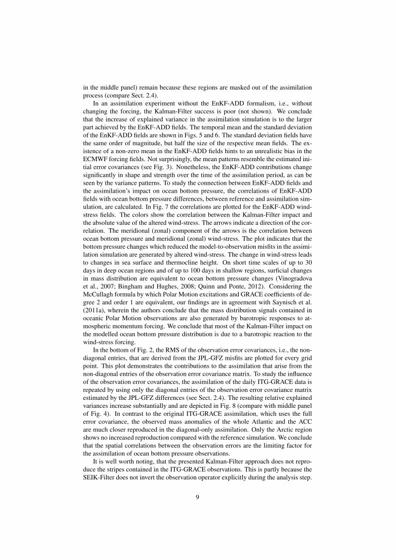
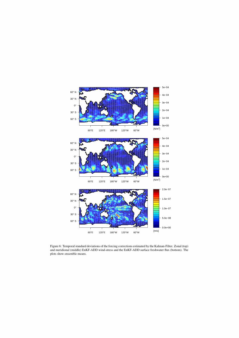
In an assimilation experiment without the EnKF-ADD formalism, i.e., withoutchanging the forcing, the Kalman-Filter success is poor (not shown). We concludethat the increase of explained variance in the assimilation simulation is to the largerpart achieved by the EnKF-ADD fields. The temporal mean and the standard deviationof the EnKF-ADD fields are shown in Figs. 5 and 6. The standard deviation fields havethe same order of magnitude, but half the size of the respective mean fields. The ex-istence of a non-zero mean in the EnKF-ADD fields hints to an unrealistic bias in theECMWF forcing fields. Not surprisingly, the mean patterns resemble the estimated ini-tial error covariances (see Fig. 3). Nonetheless, the EnKF-ADD contributions changesignificantly in shape and strength over the time of the assimilation period, as can beseen by the variance patterns. To study the connection between EnKF-ADD fields andthe assimilation’s impact on ocean bottom pressure, the correlations of EnKF-ADDfields with ocean bottom pressure differences, between reference and assimilation sim-ulation, are calculated. In Fig. 7 the correlations are plotted for the EnKF-ADD wind-stress fields. The colors show the correlation between the Kalman-Filter impact andthe absolute value of the altered wind-stress. The arrows indicate a direction of the cor-relation. The meridional (zonal) component of the arrows is the correlation betweenocean bottom pressure and meridional (zonal) wind-stress. The plot indicates that thebottom pressure changes which reduced the model-to-observation misfits in the assimi-lation simulation are generated by altered wind-stress. The change in wind-stress leadsto changes in sea surface and thermocline height. On short time scales of up to 30days in deep ocean regions and of up to 100 days in shallow regions, surficial changesin mass distribution are equivalent to ocean bottom pressure changes (Vinogradovaet al., 2007; Bingham and Hughes, 2008; Quinn and Ponte, 2012). Considering theMcCullagh formula by which Polar Motion excitations and GRACE coefficients of de-gree 2 and order 1 are equivalent, our findings are in agreement with Saynisch et al.(2011a), wherein the authors conclude that the mass distribution signals contained inoceanic Polar Motion observations are also generated by barotropic responses to at-mospheric momentum forcing. We conclude that most of the Kalman-Filter impact onthe modelled ocean bottom pressure distribution is due to a barotropic reaction to thewind-stress forcing.

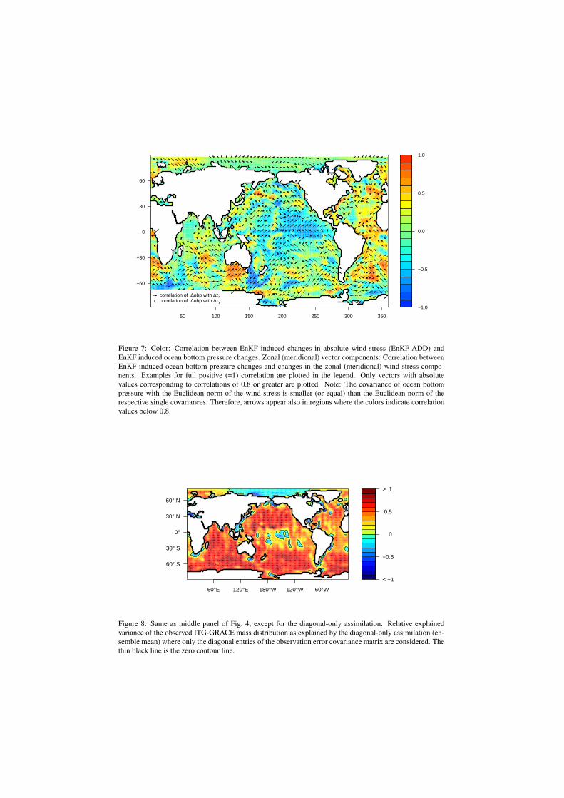
In the bottom of Fig. 2, the RMS of the observation error covariances, i.e., the non-diagonal entries, that are derived from the JPL-GFZ misfits are plotted for every gridpoint. This plot demonstrates the contributions to the assimilation that arise from thenon-diagonal entries of the observation error covariance matrix. To study the influenceof the observation error covariances, the assimilation of the daily ITG-GRACE data isrepeated by using only the diagonal entries of the observation error covariance matrixestimated by the JPL-GFZ differences (see Sect. 2.4). The resulting relative explainedvariances increase substantially and are depicted in Fig. 8 (compare with middle panelof Fig. 4). In contrast to the original ITG-GRACE assimilation, which uses the fullerror covariance, the observed mass anomalies of the whole Atlantic and the ACCare much closer reproduced in the diagonal-only assimilation. Only the Arctic regionshows no increased reproduction compared with the reference simulation. We concludethat the spatial correlations between the observation errors are the limiting factor forthe assimilation of ocean bottom pressure observations.

It is well worth noting, that the presented Kalman-Filter approach does not repro-duce the stripes contained in the ITG-GRACE observations. This is partly because theSEIK-Filter does not invert the observation operator explicitly during the analysis step.

9

To get the analysis-increment from the observations the SEIK-Filter uses a recombina-tion of the forecast-members. Therefore, the stripes are not reproduced because theyare not in the span of the leading eigenvectors of the ocean model’s cross-ensemblevariance. Or stated otherwise, the cross-ensemble variance, i.e., the ocean model error,is small in these regions compared with the estimated observation errors (see Fig. 2,top).

Because in general the destriping of the GRACE solutions is based on time-invariantstatistic assumptions, it would be interesting to develop an approach that is moredynamic and contains more physical information by incorporating an ocean model.Therefore, we study how much information our assimilation set-up can extract fromstripe contaminated observations. Since there is no respective version of ITG-GRACEavailable, a version of the GFZ solution which still contains stripes (GFZ-GRACE) isused instead. The only difference in the GFZ-GRACE processing to the one describedin Sect. 2.4 is that the destriping step is not applied. For better comparability with theITG-GRACE assimilation, the monthly GFZ-GRACE solutions (destriped and non-destriped) are interpolated to daily values using a spline approach. Since the unpro-cessed stripes are at least three orders of magnitude larger than the previously assimi-lated ocean bottom pressure signal, these three orders of magnitude must be consideredas observation error and the error budget has to be adapted accordingly. A matrix withentries of 1× 103 m2 on the diagonal and zero elsewhere is used as observation errormatrix. This number is an upper bound to typical GRACE errors of 1-3 cm (Quinn andPonte, 2008) that are increased by the three orders of magnitude which distinct typicalocean bottom pressure signals from the artificial stripes: 1×103 m2 > (0.03m×103)2.Note that, this experiment was run over the period of one year (2004) only. In the re-sulting GFZ-GRACE assimilation, no stripes are reproduced (not shown). The successof the GFZ-GRACE stripe assimilation is evaluated against the fully processed, i.e., de-striped GRACE observations from GFZ. The relative explained variances are depictedin Fig. 9. The model-to-observation agreements grow globally in the GFZ-GRACEassimilation compared with the reference simulation. The GFZ-GRACE assimilationshows pronounced agreements throughout the whole Southern Ocean and the gain inexplained variance reaches up to 80 hPa2 in the Southeast-Pacific Basin. The agree-ments are remarkable and the method can be ranked among the already existing de-striping mechanisms mentioned in Sect. 1.

3.2. Comparisons with independent ocean bottom pressure recorders

To further quantify the quality of the GRACE assimilations, we compare the modeloutput with independent, i.e., not assimilated, observations. For this comparison, datasets of in situ ocean bottom pressure recorders are used. The data was recorded byPressure Inverted Echo Sounders (PIES) and is provided by Macrander et al. (2010).The recordings are quality controlled, i.e., outliers are eliminated and drifts are reducedby a quadratic fit. Tides are removed by means of the FES2004 tide model (Lyard et al.,2006). To mimic the removal of the global mean ocean bottom pressure in the Kalman-Filter, the comparisons with the ocean model simulations take only signals of 100 daysand shorter into account, i.e., trends, annual and semi-annual signals are not containedin the recorder data and are, therefore, not part of the comparisons. It is important topoint out that PIES recorders are not evenly distributed over the ocean (Fig. 10, toppanel). Furthermore, the PIES are mostly located close to coasts or in places with com-plicated topographic or dynamic characteristic, e.g., in deep-sea trenches, the FramStrait or the Drake Passage. In addition, PIES measurements are point-measurements,

10

but ocean model grid points represent up to ten thousand square kilometers. The RMS-differences between 100 day highpass-filtered model simulations (respectively assimi-lations) and the 100 day highpass-filtered in situ recorders are displayed in Fig. 10. Thecorresponding numbers are given in Tab. 1. The global decrease in RMS-difference dueto assimilation is 0.2 hPa. The regional contributions to this value are very different. Inthe Pacific region the RMS-differences between ITG-GRACE assimilation and PIESdo not change compared with the reference simulation. One problem is that most ofthe PIES are located close to the coast where the GRACE-observations are influencedby continental leakage and the assimilation is switched off (see Sect. 2.4). A secondproblem is that many PIES are located near islands or ridges that are not resolved inthe ocean model. Furthermore, some PIES time series are not very well reproducedby the satellite GRACE observations. In Fig. 11, the time series of a PIES located inthe equatorial Pacific is plotted. This particular PIES is not close to the coast, but issituated in a shallow region with complicated bathymetry and dynamic. It can be seenthat ITG-GRACE data itself has little resemblance to the PIES observation. Conse-quently, the assimilation fails to reproduce the recorder data. In general, ocean modelsand satellite observations show insufficient sub-monthly variability in this equatorialregion (compare also with Fig. 2 of Bonin and Chambers, 2011). In the Indian and At-lantic region, there is a slight decrease of the model-to-observation misfits of up to 0.1hPa in the mean. In the high-latitude regions, there is a pronounced RMS-decrease ofup to 1.9 hPa, i.e., a decrease of 35 % (see, e.g., PIES #7, #21). The mean RMS of theregions decrease from 4.1 hPa to 3.7 hPa in the Arctic and from 3.7 hPa to 3.3 hPa in theSouthern Ocean. This pronounced impact on polar latitudes agrees with the findingsof Köhl et al. (2012) and extends them to higher frequencies. In Fig. 12, the PIES #21from the ACC region is plotted and both, ITG-GRACE and assimilation reproduce therecorder data very well. In most cases, the agreement between diagonal-only assimila-tion and PIES is better than between the original ITG-GRACE assimilation and PIES.In some cases, this relation is inverted. Here, overfitting occurs (e.g., PIES #45, #48).These PIES are located close to the North-American west coast where the original ITG-GRACE assimilation ignores the observations (see middle panel of Fig. 4). In contrastto this, the diagonal-only assimilation reproduces the ITG GRACE observations (seeFig. 8). The worse fit of the diagonal-only assimilation to PIES in this region hints tocoastal-leakage artifacts in the ITG-GRACE data. We conclude, to avoid overfittingit is important to consider the covariances of the observation errors in the assimilationprocess.

In the case of the assimilation of non-destriped GFZ-GRACE data, the same globaldependencies can be seen (Fig. 13, turquoise squares, see also Table 1). Note that,this experiment has a short time window of one year (2004) and the depicted RMScover only this period. Furthermore, not all PIES have a reasonable overlap with thatperiod. Most of the remaining model-to-PIES RMS reduce by assimilating the heav-ily striped GFZ-GRACE observations. The global mean RMS reduction amounts to0.5 hPa. At least in this short experiment, the level of agreement to the PIES data iscomparable but slightly (0.1 hPa) better than in the original ITG-GRACE assimilation(blue/white squares) and comparable but slightly (0.05 hPa) worse than in the diagonal-only ITG-GRACE assimilation (green squares). The better agreement of the diagonal-only ITG-GRACE assimilation is most pronounced in the Arctic Ocean (up to 0.6 hPa) where high-frequency signals play an important role (Quinn and Ponte, 2012, seealso Fig. 12). Nonetheless, the benefit from the assimilation of monthly non-destripeddata is remarkable. Given the very noisy observation data and the crude observationerror approximation used in this particular experiment, the results show how robust

11

the presented EnKF formalism performs if a reasonable ocean model ensemble can beconstructed.

4. Summary

Daily and monthly gravity field observations from the GRACE satellite missionare processed to derive ocean bottom pressure anomalies. These observations are as-similated with a dynamic global ocean circulation model. The daily observations areassimilated for the period 2003 to 2009. The monthly data is assimilated for the year2004. The assimilation method is an ensemble based Kalman-Filter that operates on asmall, but optimal subspace of the model’s state space. Variances and covariances ofthe initial model state errors are estimated and incorporated into the filter. To considererrors in the atmospheric forcing, i.e., wind-stress and freshwater-flux, the Kalman-Filter is extended to employ an ensemble of individual forcings. Variances and covari-ances of the GRACE observation errors are estimated. The assimilation experimentsare calculated with and without use of the observation error covariance information.

Compared with a reference simulation, the assimilation of GRACE data leads toincreased agreement between modelled ocean bottom pressure fields and the oceanbottom pressure fields observed by GRACE. The global mean correlation rises from0.15 to 0.36. The physical explanation for the higher correlations are found in wind-stress changes which are generated by the assimilation of GRACE data. These changesgenerate barotropic signals which influence the ocean bottom pressure fields.

Apart from reproducing the GRACE observations, the presented Kalman-Filter ap-proach shows great potential in reducing the artificial stripes that contaminate GRACEobservations. The assimilation of non-destriped GRACE data shows similar results asthe assimilation of destriped GRACE data. The reason is the EnKF’s rejection of fea-tures that lay outside the leading eigenvectors of the model’s cross-ensemble variance.This is an advantage over other, e.g., adjoint, assimilation methods.

In addition, the assimilation simulations show increased agreement to independent,i.e., not assimilated observations from in situ ocean bottom pressure recorders. In ourassimilation, RMS-differences reduce by up to 35 %. The improvements are most pro-nounced in the high latitudes. In the comparison with bottom pressure recorders, theassimilation of daily ITG solutions leads to slightly better results than the assimilationof monthly GRACE data. The reproduction of satellite and in situ ocean mass obser-vations is limited by the observation error budget and especially, by the error’s cor-relations. Assimilation experiments under the assumption of uncorrelated observationerrors show substantially increased agreement to the assimilated satellite observationsand moderate increased agreement to the independent in situ observations. The com-parison to the bottom pressure recorders shows that the information contained in theobservation error correlations can prevent the assimilation from overfitting.

Since in fact the GRACE observation errors are correlated and good destriping al-gorithms already exist, these benchmark experiments could be considered dispensablebut they demonstrate the power and robustness of the applied filter technique when areasonable model is constructed. Furthermore, the experiments show what informationcan be extracted from the observations if future satellite missions or coming process-ing techniques could decrease the observation’s errors and especially their correlations.The presented assimilation framework will be improved in future studies by a dynami-cal approach to the error budget of the forcings and the observations. Furthermore, untilthe observation and processing errors become smaller, the application of localized errorbudgets should be considered.

12

Acknowledgements

We thank Lars Nerger for his insightful comments and the opportunity to use hisParallel Data Assimilation Framework. This study could not have been done withoutERA-Interim data provided by the ECMWF, GRACE data from the ITG, the CSR, theJPL and the GFZ and the ocean bottom pressure recorder observations provided byAndreas Macrander. The model simulations are calculated at the German ClimateComputing Center and the study was funded by the German Research Foundation,which is much appreciated.

References

I. Bergmann, H. Dobslaw, Short-term transport variability of the Antarctic CircumpolarCurrent from satellite gravity observations. J. Geophys. Res.-Oceans 117, 05044(2012)

R.J. Bingham, C.W. Hughes, The relationship between sea-level and bottom pressurevariability in an eddy permitting ocean model. Geophys. Res. Lett. 35(3), 03602(2008)

J.A. Bonin, D.P. Chambers, Evaluation of high-frequency oceanographic signal inGRACE data: Implications for de-aliasing. Geophys. Res. Lett. 38, 17608 (2011)

A. Cazenave, J. Chen, Time-variable gravity from space and present-day mass redistri-bution in the Earth system. Earth Planet. Sci. Lett. 298(3-4), 263–274 (2010)

D.P. Chambers, Evaluation of new GRACE time-variable gravity data over the ocean.Geophys. Res. Lett. 33(17), 17603 (2006)

D.P. Chambers, J.A. Bonin, Evaluation of Release-05 GRACE time-variable gravitycoefficients over the ocean. Ocean Sci. 8(5), 859–868 (2012)

A.H. Chaudhuri, M.R. Ponte, G. Forget, P. Heimbach, A comparison of atmosphericreanalysis surface products over the ocean and implications for uncertainties in air-sea boundary forcing. J. Climate 26, 153–170 (2013)

R. Dill, Hydrological model LSDM for operational Earth rotation and gravity field vari-ations, Technical Report STR08/09, Helmholtz-Zentrum Potsdam Deutsches Geo-ForschungsZentrum, 2008

H. Dobslaw, M. Thomas, Simulation and observation of global ocean mass anomalies.J. Geophys. Res. Oceans 112(C05040), 05040 (2007)

R. Eanes, SLR solutions from the University of Texas Center for Space Research, Geo-center from TOPEX SLR/DORIS, 1992-2000, http://sbgg.jpl.nasa.gov/dataset.html,2000. IERS Spec. Bur. for Gravity/Geocent., Pasadena, Calif.

F. Flechtner, AOD1B product description document, GRACE 327-750, rev. 3.1, Tech-nical report, GFZ German Research Centre for Geosciences, 2007

R.J. Greatbatch, A note on the representation of steric sea-level in models that conservevolume rather than mass. J. Geophys. Res.-Oceans 99(C6), 12767–12771 (1994)

13

A. Köhl, F. Siegismund, D. Stammer, Impact of assimilating bottom pressure anomaliesfrom grace on ocean circulation estimates. J. Geophys. Res. 117, 04032 (2012)

E. Kurtenbach, A. Eicker, T. Mayer-Guerr, M. Holschneider, M. Hayn, M. Fuhrmann,J. Kusche, Improved daily GRACE gravity field solutions using a Kalman smoother.J. Geodyn. 59(SI), 39–48 (2012)

J. Kusche, Approximate decorrelation and non-isotropic smoothing of time-variableGRACE-type gravity field models. J. Geodesy 81(11), 733–749 (2007)

F. Lyard, F. Lefevre, T. Letellier, O. Francis, Modelling the global ocean tides: moderninsights from FES2004. Ocean Dyn. 56(5-6), 394–415 (2006)

A. Macrander, C. Böning, O. Boebel, J. Schröter, Validation of GRACE GravityFields by In-Situ Data of Ocean Bottom Pressure, in System Earth via Geodetic-Geophysical Space Techniques, ed. by F.M. Flechtner, T. Gruber, A. Güntner, M.Mandea, M. Rothacher, T. Schöne, J. Wickert Advanced Technologies in EarthSciences (Springer Berlin Heidelberg, ???, 2010), pp. 169–185. ISBN 978-3-642-10227-1

L. Nerger, W. Hiller, Software for ensemble-based data assimilation systems - imple-mentation strategies and scalability. J. Cageo 55, 110–118 (2012)

L. Nerger, S. Danilov, G. Kivman, W. Hiller, J. Schröter, Data assimilation with theEnsemble Kalman Filter and the SEIK filter applied to a finite element model of theNorth Atlantic. J. Mar. Syst. 65(1-4), 288–298 (2007)

D.T. Pham, Stochastic methods for sequential data assimilation in strongly nonlinearsystems. Mon. Weather Rev. 129(5), 1194–1207 (2001)

D.T. Pham, J. Verron, L. Gourdeau, Singular evolutive Kalman filters for data assimila-tion in oceanography. Comptes Rendus Acad. Sci. Ser. II A 326(4), 255–260 (1998)

K.J. Quinn, R.M. Ponte, Estimating weights for the use of time-dependent gravity re-covery and climate experiment data in constraining ocean models. J. Geophys. Res.-Oceans 113(C12), 12013 (2008)

K.J. Quinn, R.M. Ponte, Uncertainty in ocean mass trends from GRACE. Geophys. J.Int. 181(2), 762–768 (2010)

K.J. Quinn, R.M. Ponte, Estimating high frequency ocean bottom pressure variability.Geophys. Res. Lett. 38, 08611 (2011)

K.J. Quinn, R.M. Ponte, High frequency barotropic ocean variability observed byGRACE and satellite altimetry. Geophys. Res. Lett. 39, 07603 (2012)

C. Sakumura, S. Bettadpur, S. Bruinsma, Ensemble prediction and intercomparisonanalysis of GRACE time-variable gravity field models. J. Geophys. Res. 41(5),1389–1397 (2014)

I. Sasgen, Z. Martinec, J. Bamber, Combined GRACE and InSAR estimate of WestAntarctic ice mass loss. J. Geophys. Res.-Earth Surf. 115, 04010 (2010)

J. Saynisch, M. Thomas, Ensemble Kalman-Filtering of Earth rotation observationswith a global ocean model. J. Geodyn. 62, 24–29 (2011)

14

J. Saynisch, M. Wenzel, J. Schröter, Assimilation of Earth rotation parameters into aglobal ocean model: excitation of polar motion. Nonlinear Process. Geophys. 18(5),581–585 (2011a)

J. Saynisch, M. Wenzel, J. Schröter, Assimilation of Earth rotation parameters into aglobal ocean model: length of day excitation. J. Geodesy 85(2), 67–73 (2011b)

E.J.O. Schrama, B. Wouters, Revisiting Greenland ice sheet mass loss observed byGRACE. J. Geophys. Res.-Solid Earth 116, 02407 (2011)

H. Steffen, S. Petrovic, J. Mueller, R. Schmidt, J. Wuensch, F. Barthelmes, J. Kusche,Significance of secular trends of mass variations determined from GRACE solutions.J. Geodyn. 48(3-5, SI), 157–165 (2009)

H.v. Storch, F.W. Zwiers, Statistical Analysis in Climate Research (Cambridge Univer-sity Press, ???, 1999), p. 484

S. Swenson, J. Wahr, Post-processing removal of correlated errors in GRACE data.Geophys. Res. Lett. 33(8), 08402 (2006)

M. Thomas, J. Sündermann, E. Maier-Reimer, Consideration of ocean tides in anOGCM and impacts on subseasonal to decadal polar motion excitation. Geophys.Res. Lett. 28(12), 2457–2460 (2001)

K.E. Trenberth, J.T. Fasullo, J. Mackaro, Atmospheric moisture transports from oceanto land and global energy flows in reanalyses. J. Clim. 24(18), 4907–4924 (2011)

S. Uppala, D. Dee, S. Kobayashi, P. Berrisford, A. Simmons, Toward a climate data as-similation system: Status update of ERA Interim, Technical report, ECMWF Newsl.,2008

M.L. Vianna, V.V. Menezes, D.P. Chambers, A high resolution satellite-only GRACE-based mean dynamic topography of the South Atlantic Ocean. Geophys. Res. Lett.34(24), 24604 (2007)

N.T. Vinogradova, R.M. Ponte, D. Stammer, Relation between sea level and bottompressure and the vertical dependence of oceanic variability. Geophys. Res. Lett.34(3), 03608 (2007)

J. Wahr, M. Molenaar, F. Bryan, Time variability of the Earth’s gravity field: Hydro-logical and oceanic effects and their possible detection using GRACE. J. Geophys.Res. 103(B12), 30205–30229 (1998)

M. Wenzel, J. Schröter, The global ocean mass budget in 1993-2003 estimated fromsea level change. J. Phys. Oceanogr. 37(2), 203–213 (2007)

S. Werth, A. Guentner, R. Schmidt, J. Kusche, Evaluation of GRACE filter tools froma hydrological perspective. Geophys. J. Int. 179(3), 1499–1515 (2009)

J.K. Willis, D.P. Chambers, R.S. Nerem, Assessing the globally averaged sea level bud-get on seasonal to interannual timescales. J. Geophys. Res.-Oceans 113(C6), 06015(2008)

15

OMCT ensemble (day i)

Additional forcing ensemble (day i)

+

OMCT ensemble (day i+1)

GRACE data

time

ECMWF Interim Forcing

Additional forcing ensemble (day i+1)

Kalman Filter

Figure 1: Schematic of this study’s ensemble based Kalman-Filter configuration and time stepping.

0

1

2

3

4

5

6

> 7

60°E 120°E 180°W 120°W 60°W

60° S

30° S

0°

30° N

60° N

[hPa2]

0

1

2

3

4

5

60°E 120°E 180°W 120°W 60°W

60° S

30° S

0°

30° N

60° N

[hPa2]

Figure 2: Estimated error budget of the assimilated GRACE observations. Variances of the JPL-GFZ misfit(top). RMS-values of the covariances, i.e., the nondiagonal entries of the observation error covariance matrix(bottom).

0e+00

1e−08

2e−08

3e−08

4e−08

5e−08

60°E 120°E 180°W 120°W 60°W

60° S

30° S

0°

30° N

60° N

[N2/m4]

0e+00

1e−08

2e−08

3e−08

4e−08

5e−08

60°E 120°E 180°W 120°W 60°W

60° S

30° S

0°

30° N

60° N

[N2/m4]

0.0e+00

5.0e−15

1.0e−14

1.5e−14

60°E 120°E 180°W 120°W 60°W

60° S

30° S

0°

30° N

60° N

[m2/s2]

Figure 3: Estimated initial error variances of the EnKF-ADD fields, i.e., the initial EnKF-ADD cross-ensemble variances. Zonal wind-stress (top), meridional wind-stress (middle) and freshwater flux (bottom).

< −1

−0.5

0

0.5

> 1

60°E 120°E 180°W 120°W 60°W

60° S

30° S

0°

30° N

60° N

< −1

−0.5

0

0.5

> 1

60°E 120°E 180°W 120°W 60°W

60° S

30° S

0°

30° N

60° N

< −1

−0.5

0

0.5

> 1

60°E 120°E 180°W 120°W 60°W

60° S

30° S

0°

30° N

60° N

Figure 4: Relative explained variance of the observed ITG-GRACE mass distribution as explained by thereference simulation (top), as explained by the assimilation simulation (ensemble mean, middle) and thedifferences, i.e., the gain in relative explained variance by the assimilation simulation (bottom). The thinblack line is the zero contour line.

−1e−03

−5e−04

0e+00

5e−04

1e−03

60°E 120°E 180°W 120°W 60°W

60° S

30° S

0°

30° N

60° N

[N/m2]

−1e−03

−5e−04

0e+00

5e−04

1e−03

60°E 120°E 180°W 120°W 60°W

60° S

30° S

0°

30° N

60° N

[N/m2]

−4e−07

−2e−07

0e+00

2e−07

4e−07

60°E 120°E 180°W 120°W 60°W

60° S

30° S

0°

30° N

60° N

[m/s]

Figure 5: Temporal mean of the forcing corrections estimated by the Kalman-Filter. Zonal (top) and meridi-onal (middle) EnKF-ADD wind-stress and the EnKF-ADD surface freshwater flux (bottom). The plots showensemble means.

0e+00

1e−04

2e−04

3e−04

4e−04

5e−04

60°E 120°E 180°W 120°W 60°W

60° S

30° S

0°

30° N

60° N

[N/m2]

0e+00

1e−04

2e−04

3e−04

4e−04

5e−04

60°E 120°E 180°W 120°W 60°W

60° S

30° S

0°

30° N

60° N

[N/m2]

0.0e+00

5.0e−08

1.0e−07

1.5e−07

2.0e−07

60°E 120°E 180°W 120°W 60°W

60° S

30° S

0°

30° N

60° N

[m/s]

Figure 6: Temporal standard deviations of the forcing corrections estimated by the Kalman-Filter. Zonal (top)and meridional (middle) EnKF-ADD wind-stress and the EnKF-ADD surface freshwater flux (bottom). Theplots show ensemble means.

−1.0

−0.5

0.0

0.5

1.0

50 100 150 200 250 300 350

−60

−30

0

30

60

correlation of ∆obp with ∆τxcorrelation of ∆obp with ∆τy

Figure 7: Color: Correlation between EnKF induced changes in absolute wind-stress (EnKF-ADD) andEnKF induced ocean bottom pressure changes. Zonal (meridional) vector components: Correlation betweenEnKF induced ocean bottom pressure changes and changes in the zonal (meridional) wind-stress compo-nents. Examples for full positive (=1) correlation are plotted in the legend. Only vectors with absolutevalues corresponding to correlations of 0.8 or greater are plotted. Note: The covariance of ocean bottompressure with the Euclidean norm of the wind-stress is smaller (or equal) than the Euclidean norm of therespective single covariances. Therefore, arrows appear also in regions where the colors indicate correlationvalues below 0.8.

< −1

−0.5

0

0.5

> 1

60°E 120°E 180°W 120°W 60°W

60° S

30° S

0°

30° N

60° N

Figure 8: Same as middle panel of Fig. 4, except for the diagonal-only assimilation. Relative explainedvariance of the observed ITG-GRACE mass distribution as explained by the diagonal-only assimilation (en-semble mean) where only the diagonal entries of the observation error covariance matrix are considered. Thethin black line is the zero contour line.

< −1

−0.5

0

0.5

> 1

60°E 120°E 180°W 120°W 60°W

60° S

30° S

0°

30° N

60° N

< −1

−0.5

0

0.5

> 1

60°E 120°E 180°W 120°W 60°W

60° S

30° S

0°

30° N

60° N

< −1

−0.5

0

0.5

> 1

60°E 120°E 180°W 120°W 60°W

60° S

30° S

0°

30° N

60° N

Figure 9: Same as Fig. 4, except for the assimilation of non-destriped GFZ-GRACE data. Relative explainedvariance of the destriped GFZ-GRACE mass distribution as explained by the reference simulation (top),as explained by the assimilation simulation (ensemble mean, middle) and the differences, i.e., the gain inrelative explained variance by the assimilation simulation (bottom). The thin black line is the zero contourline.

60˚

60˚

120˚

120˚

180˚

180˚

−120˚

−120˚

−60˚

−60˚

0˚

0˚

−90˚ −90˚

−60˚ −60˚

−30˚ −30˚

0˚ 0˚

30˚ 30˚

60˚ 60˚

90˚ 90˚1

6

89

13

14

16

17 19

24

27

3233

36

37

39

40

44

46

51

52 53

54

59

63

2

22

29

49

4 5

1521

2526

34

35 38

5055

47

3

6162

2830

43

5657

4845

58

71012

18

20

23

31

41

42

11

60

0

1

2

3

4

5

6

Arctic

# 1−5

Southern Ocean

# 6−21

Indian

# 22

Pacific Ocean

# 23−53

Atlantic Ocean

# 54−63

100 days high pass

RM

S [h

Pa]

reference run assimilation run assimilation run (RL05)

Figure 10: Geographical location of the utilized Pressure Inverted Echo Sounders (PIES, top) and RMS-differences for 2003-2009 between modelled ocean bottom pressure and in situ recordings by PIES (bottom).RMS-differences between PIES and reference simulation (red), between PIES and assimilation simulation(ensemble mean, blue/white) and between PIES and diagonal-only assimilation simulation (ensemble mean,green).

01/08 02/08 03/08 04/08 05/08 06/08 07/08 08/08 09/08 10/08 11/08 12/08 01/09−10

−5

0

5

10

pres

sure

ano

mal

ies

[hP

a]

Station 27 − DART 52403 (Pacific−equator): 100 days high pass

residual RMS: 1.85 hPa

reference

01/08 02/08 03/08 04/08 05/08 06/08 07/08 08/08 09/08 10/08 11/08 12/08 01/09−10

−5

0

5

10

pres

sure

ano

mal

ies

[hP

a]

residual RMS: 1.86 hPa

assimilation

01/08 02/08 03/08 04/08 05/08 06/08 07/08 08/08 09/08 10/08 11/08 12/08 01/09−10

−5

0

5

10

pres

sure

ano

mal

ies

[hP

a]

residual RMS: 1.81 hPa

ITG−Grace

Figure 11: Ocean bottom pressure anomalies. In situ data from PIES #27 (DART 52403, equatorial Pacific,black). Reference simulation (red). Diagonal-only assimilation simulation (ensemble mean, green). ITG-GRACE observations (gold).

01/07 02/07 03/07 04/07 05/07 06/07 07/07 08/07 09/07 10/07 11/07 12/07 01/08−18

−12

−6

0

6

12

18

pres

sure

ano

mal

ies

[hP

a]

Station 21 − AWI ANT13a (Southern Ocean): 100 days high pass

residual RMS: 5.40 hPa

reference

01/07 02/07 03/07 04/07 05/07 06/07 07/07 08/07 09/07 10/07 11/07 12/07 01/08−18

−12

−6

0

6

12

18

pres

sure

ano

mal

ies

[hP

a]

residual RMS: 3.51 hPa

assimilation

01/07 02/07 03/07 04/07 05/07 06/07 07/07 08/07 09/07 10/07 11/07 12/07 01/08−18

−12

−6

0

6

12

18

pres

sure

ano

mal

ies

[hP

a]

residual RMS: 2.63 hPa

ITG−Grace

Figure 12: Ocean bottom pressure anomalies. In situ data from PIES #21 (AWI ANT13a, Southern Ocean,black). Reference simulation (red). Diagonal-only assimilation simulation (ensemble mean, green). ITG-GRACE observations (gold).

0

1

2

3

4

5

6

Arctic

# 1−5

Southern Ocean

# 6−21

Indian

# 22

Pacific Ocean

# 23−53

Atlantic Ocean

# 54−63

100 days high pass

RM

S [h

Pa]

reference run assimilation run (non−destriped) assimilation run assimilation run (RL05)

Figure 13: RMS-differences for 2004 between modelled ocean bottom pressure and in situ recordings byPIES, between PIES and reference simulation (red), between PIES and assimilation simulation (ensemblemean, blue/white), between PIES and diagonal-only assimilation simulation (ensemble mean, green) and be-tween PIES and assimilation of non-destriped GRACE data (ensemble mean, turquois). For the geographicallocation of the PIES see Fig. 10.

Station No. Data corresponding to 2003-2009 (Fig. 10) Data corresponding to 2004 (Fig. 13)ref assim diag-only ref assim diag-only GFZ-assim

Arc

ticO

cean

1 4.24 4.25 3.78 5.37 5.06 4.41 4.732 3.92 3.91 3.20 4.80 4.35 3.82 4.383 3.64 3.64 2.87 - - - -4 4.10 4.05 4.03 - - - -5 4.66 4.61 4.62 - - - -

mean 4.11 4.09 3.70 5.09 4.70 4.12 4.56

Sout

hern

Oce

an

6 4.32 4.15 3.51 5.40 5.06 3.75 3.607 5.28 4.94 3.61 - - - -8 3.16 3.02 2.79 - - - -9 3.66 3.56 2.73 - - - -

10 2.92 2.84 2.43 - - - -11 2.77 2.70 2.36 3.51 2.98 2.36 2.9212 3.34 3.32 3.26 - - - -13 7.25 7.23 7.29 - - - -14 2.80 2.78 2.58 4.25 3.38 3.04 3.0115 2.51 2.52 2.47 3.65 2.65 2.46 2.5616 2.27 2.16 1.93 - - - -17 3.18 3.18 3.20 3.78 3.68 3.79 3.6218 3.01 2.98 2.98 3.87 3.23 3.35 3.1419 4.12 4.10 4.13 5.13 4.17 4.26 4.1420 3.39 3.35 3.41 3.78 3.42 3.41 3.3721 5.40 4.12 3.51 - - - -

mean 3.71 3.56 3.26 4.17 3.57 3.30 3.30

Ind. O. 22 2.21 2.22 2.10 - - - -

Paci

ficO

cean

23 1.71 1.73 1.75 - - - -24 1.78 1.77 1.74 - - - -25 1.88 1.94 1.90 1.63 1.81 1.78 1.7526 1.43 1.44 1.44 1.55 1.42 1.45 1.3627 1.85 1.84 1.86 - - - -28 3.77 3.79 3.77 2.53 2.36 2.21 2.3129 3.16 3.17 3.29 3.27 3.49 3.59 3.5130 3.74 3.76 3.82 - - - -31 2.07 2.03 2.03 - - - -32 1.70 1.69 1.77 - - - -33 1.57 1.59 1.62 - - - -34 2.18 2.20 2.19 - - - -35 2.04 2.05 1.94 - - - -36 1.60 1.62 1.61 - - - -37 3.34 3.36 3.17 - - - -38 3.38 3.37 3.55 - - - -39 1.81 1.80 1.86 - - - -40 2.94 2.99 2.87 - - - -41 1.90 1.80 1.88 - - - -42 3.73 3.75 3.75 4.42 3.85 3.81 3.8243 3.56 3.59 3.63 4.38 3.84 3.72 3.8744 1.84 1.81 1.78 - - - -45 1.51 1.51 1.72 2.02 1.99 1.95 1.7546 2.72 2.70 2.86 - - - -47 4.25 4.24 4.19 - - - -48 2.58 2.58 2.74 - - - -49 3.52 3.53 3.58 - - - -50 1.33 1.33 1.47 - - - -51 2.71 2.72 2.72 - - - -52 1.56 1.54 1.51 - - - -53 1.40 1.41 1.43 - - - -

mean 2.40 2.41 2.43 2.81 2.68 2.64 2.63

Atla

ntic

Oce

an

54 1.94 1.93 1.87 - - - -55 4.62 4.67 4.16 - - - -56 4.82 4.84 4.81 - - - -57 4.46 4.49 4.44 - - - -58 2.46 2.44 2.41 - - - -59 1.88 1.86 1.92 - - - -60 2.39 2.38 2.35 2.55 2.10 1.95 2.0561 1.98 1.96 1.88 2.48 2.05 1.97 2.0962 2.11 2.08 2.00 2.44 2.11 2.09 2.1463 5.46 5.45 5.46 - - -

mean 3.21 3.21 3.13 2.49 2.06 2.00 2.09

global mean 3.00 2.96 2.85 3.54 3.15 2.96 3.01

Table 1: RMS-differences [hPa] between modelled ocean bottom pressure and in situ recordings by PIES.