grand canonical ensembles in general relativity
TRANSCRIPT

Grand canonical ensembles in general relativity
David Klein1 and Wei-Shih Yang2
We develop a formalism for general relativistic, grand canonical ensembles in
space-times with timelike Killing fields. Using that, we derive ideal gas laws,
and show how they depend on the geometry of the particular space-times.
A systematic method for calculating Newtonian limits is given for a class of
these space-times, which is illustrated for Kerr space-time. In addition, we
prove uniqueness of the infinite volume Gibbs measure, and absence of phase
transitions for a class of interaction potentials in anti-de Sitter space.
KEY WORDS: relativistic Gibbs state, Fermi coordinates, grand canonical
ensemble, ideal gas, anti-de Sitter space, de-Sitter space, Einstein static
universe, Kerr space-time
Mathematics Subject Classification: 82B21, 83C15, 83F05
1Department of Mathematics and Interdisciplinary Research Institute for the Sci-ences, California State University, Northridge, Northridge, CA 91330-8313. Email:[email protected].
2Department of Mathematics, Temple University, Philadelphia, PA 19122. Email:[email protected].

1. Introduction
Newtonian infinite volume grand canonical Gibbs measures on Riemannian man-ifolds have been studied for more than a decade [1, 2, 3, 4]. Recently, in thecontext of general relativity, the finite volume canonical ensemble was developedand compared to Newtonian analogs for an ideal gas of test particles, providedthat the container of gas is within the range of validity of Fermi coordinates foran observer whose worldline follows a timelike Killing vector, and the containeris stationary relative to the observer [5].
Here we consider grand canonical ensembles, with the assumption that the testparticles constituting the gas or fluid do not affect the background metric ten-sor. One might expect that the theory of specifications and Gibbs states forRiemannian manifolds developed in [1, 2, 3], and the references therein, couldbe applied in a straightforward manner to Lorentzian space-time manifolds, thusproviding a framework for general relativistic statistical mechanics. However,there are several impediments. First, space-time and energy-momentum coor-dinates are not easily decoupled as in the Newtonian case. One must work fromthe start with the cotangent bundle of space-time. In some spacetimes thereis a nonzero energy of the vacuum that must be accounted for in a thermody-namic formalism. There are also ambiguities associated with the notion of athermodynamic limit, since space-time can be foliated into space slices along anobserver’s timelike path in many different ways. In addition, the notion of po-tential energy, which is a feature of central importance in statistical mechanics,normally has no place in general relativity. These issues are considered in thesequel.
For the purposes of statistical mechanics, our requirement that the spacetimepossess a timelike Killing field is natural. The Killing vector field, tangent tothe timelike path of an observer, determines a time coordinate for the system,and thus an energy component of the four-momentum. As a consequence, com-parisons to corresponding non relativistic statistical mechanical formulas arepossible in some space-times for certain observers. Moreover, this choice offour-velocity forces the particle system to evolve in such a way that the geome-try of spacetime is unchanging along its worldsurface (since the Lie derivative ofthe metric vanishes in that direction), making it plausible on physical groundsfor the system to reach equilibrium.
The significance of the frame of reference in relativistic statistical mechanics wasdiscussed in [5]. Even in Minkowski space-time, there is no Lorentz invariantthermal state for an ideal gas system. A thermal state is in equilibrium only ina preferred Lorentz frame in which the container of gas is at rest, and thereforebreaks Lorentz invariance [6]. The natural generalization for statistical mechan-ics in a space-time with a timelike Killing field is an orthonormal tetrad in whichthe Killing vector determines the time axis.
2
In Sect. 2 of this paper, we develop a non rotating, orthonormal “Fermi-Walker-Killing” coordinate system in which the Killing vector serves as the time axis.The measure on phase space based on these coordinates satisfies a Liouville the-orem and is invariant under space coordinate transformations. Sect. 3 appliesthe grand canonical formalism already available for Riemannian manifolds tothe Fermi surface defined in the previous section, and establishes notation. Sect.4 provides a general relativistic ideal gas law. The term “ideal gas” is some-what misleading in the context of general relativity. This is because a volumeof gas subject to no forces is still affected by the curvature of space-time, andthis corresponds to a Newtonian gas subject to gravitational, tidal, and in someinstances “centrifugal forces,” but otherwise “ideal.”
In Sect. 5, we define “Newtonian limit” as the limit of statistical mechanicalquantities as the speed of light c→∞ for a class of spacetimes whose timelikeKilling fields have a certain dependence on c. We prove convergence of relativis-tic Gibbs states evaluated on cylinder sets to their Newtonian counterparts forthe ideal gas case, and define associated Newtonian pressures. This Newtonianlimit is illustrated in detail in Sect. 6 for a gas of particles following a circularorbit in Kerr space-time. In Sect. 7, we prove uniqueness of the infinite volumeGibbs state in anti-de Sitter space for a class of equilibrium interaction poten-tials and calculate the infinite volume relativistic pressure for an ideal gas oftest particles. Concluding remarks are given in Sect. 8.
2. Particle systems on space-time manifolds
Let (M, g) be a smooth four-dimensional Lorentzian manifold. The Levi-Civitaconnection is denoted by ∇, and throughout we use the sign conventions ofMisner, Thorne and Wheeler [7]. Let σ(τ) be a a timelike path parameterizedby proper time τ with unit tangent vector e0(τ). The path, σ(τ), represents theworldline of an observer, who (in principle) may make measurements.
Measurements in a gravitational field are most easily interpreted through theuse of a system of locally inertial coordinates. For the observer σ(τ), Fermi-Walker coordinates provide such a system. A Fermi-Walker coordinate frame isnonrotating in the sense of Newtonian mechanics and is realized physically asa system of gyroscopes [7, 8, 9, 10]. Expressed in these coordinates, the met-ric along the path is Minkowskian, with first order corrections away from thepath that depend only on the four-acceleration of the observer. If the path isgeodesic, the coordinates are commonly referred to as Fermi or Fermi normalcoordinates, and the metric is Minkowskian to first order near the path withsecond order corrections due only to curvature of the space-time [7]. A partiallisting of the numerous applications of Fermi-Walker coordinates is given in [11] .
3
A Fermi-Walker coordinate system for σ may be constructed as follows. Avector field ~v inM is said to be Fermi-Walker transported along σ if ~v satisfiesthe Fermi-Walker equations given in coordinate form by,
Fe0(vα) ≡ ∇e0 vα + Ωαβvβ = 0 . (1)
where Ωαβ = aαuβ − uαaβ , and aα is the four-acceleration along σ. A Fermi-Walker coordinate system along σ is determined by an orthonormal tetrad ofvectors, e0(τ), e1(τ), e2(τ), e3(τ) Fermi-Walker transported along σ. Fermi-Walker coordinates x0, x1, x2, x3 relative to this tetrad are defined by,
x0(
expσ(τ)(λjej(τ)
)= τ
xk(
expσ(τ)(λjej(τ)
)= λk,
(2)
where here and below, Greek indices run over 0, 1, 2, 3 and Latin over 1, 2, 3.The exponential map, expp(~v), denotes the evaluation at affine parameter 1 ofthe geodesic starting at the point p in the space-time, with initial derivative ~v,and it is assumed that the λj are sufficiently small so that the exponential mapsin Eq.(2) are defined. From the theory of differential equations, a solution tothe geodesic equations depends smoothly on its initial data so it follows fromEq.(2) that Fermi-Walker coordinates are smooth. Moreover, it follows from[12] that there exists a neighborhood of σ on which the map χ = (x0, x1, x2, x3)is a diffeomorphism onto an open set in R4 and hence a coordinate chart. Gen-eral formulas in the form of Taylor expansions for coordinate transformationsto and from Fermi-Walker coordinates, are given in [13].
Assume now that ~K is a timelike Killing vector field in a neighborhood of σ andthe tangent vector to σ is ~K, i.e., e0 = ~K. The vector field ~K is the infinitesimalgenerator of a local one-parameter group φs of diffeomorphisms. The functionφs is the flow with tangent vector ~K at each point, and σ(τ) = φτ (0, 0, 0, 0)(where (0, 0, 0, 0) is the origin in Fermi-Walker coordinates).
Following [5], define a diffeomorphism χ−1 from a sufficiently small neighbor-hood of the origin in R4 to a neighborhood U of σ(0) in M by
χ−1(x0, x1, x2, x3) ≡ φx0(χ−1(0, x1, x2, x3)) (3)
Then χ = (x0, x1, x2, x3) is a coordinate system on U which, as in [5], we referto as Fermi-Walker-Killing coordinates. It follows that,
4
(0, x1, x2, x3) = (0, x1, x2, x3)
∂
∂xi
∣∣∣x0=0
=∂
∂xi
∣∣∣x0=0
∂
∂x0= ~K.
(4)
Thus, in Fermi-Walker-Killing coordinates, the time coordinate x0 is the pa-rameter of the flow generated by the Killing field ~K with initial positions of theform (0, x1, x2, x3) in Fermi-Walker coordinates.
In the case of Fermi-Walker coordinates we designate momentum form coordi-nates as pα and in the case of Fermi-Walker-Killing coordinates, the momentumform coordinates will be designated as pα. Thus, coordinates of the cotangentbundle ofM will be represented as xα, pβ or xα, pβ. The metric componentsin Fermi-Walker coordinates are designated as gαβ and in Fermi-Walker-Killingcoordinates as gαβ . Note that gαβ does not depend on x0 because of Eqs.(4).
The state of a single particle consists of its four space-time coordinates togetherwith its four-momentum coordinates xα, pβ, but the one-particle Hamiltoniansatisfies,
H =1
2gαβ pαpβ = −m
2c2
2, (5)
where, for timelike geodesics, m is the rest mass of the particle, and c is the speedof light. Eq.(5) just states the standard fact from relativity that the square ofthe “norm” of the four-velocity of a timelike particle is -1. An arbitrary choiceof p1, p2, p3, determines p0 by,
p0 =−g0ipi +
√(g0j g0k − g00gjk)pj pk − g00m2c2
g00, (6)
so that Eq.(5) holds.
Let ϕ :M→ R by,
ϕ(x) = g(exp−1σ(0) x, σ
′(0)). (7)
The space slice, X, at time coordinate τ = 0 = x0, orthogonal to the observer’sfour-velocity (along σ(τ)) is given by,
X ≡ ϕ−1(0). (8)
5
The restriction 3g of the space-time metric g to X makes (X,3 g) a Riemannianmanifold, sometimes referred to as a Fermi surface or Landau submanifold, c.f.,for example, [14] and references therein.
Remark 1. The Fermi surface X defines the collection of space-time pointsthat are simultaneous with σ(0) in a natural way relative to the observer σ.Hypersurfaces parallel to X foliate a (possibly global) neighborhood of σ, anddefine a notion of simultaneity. This foliation has been used to study geometri-cally defined relative velocities of distant objects and time dependent diametersof Robertson-Walker cosmologies [15, 16]
Thus, using Eq.(6), the phase space for a single particle at time coordinatex0 = 0 is determined by the Fermi surface, X, together with the associatedmomentum coordinates, i.e., the cotangent bundle of the Fermi surface at fixedtime coordinate x0. Let P be the sub bundle of the cotangent bundle of space-time with each three dimensional fiber determined by (6). The proof of thefollowing proposition is given in [17].
Proposition 1. The volume 7-form ω on P given by,
ω =1
p0dx0 ∧ dx1 ∧ dx2 ∧ dx3 ∧ dp1 ∧ dp2 ∧ dp3, (9)
is invariant under all coordinate transformations.
As discussed in [5], phase space for a single particle is determined by the Fermisurface, at fixed time coordinate, orthogonal to the observer’s four-velocity(along σ(τ)), along with the associated momentum coordinates, i.e., the cotan-gent bundle of the Fermi surface at fixed time coordinate x0. The appropriatevolume form is given by the interior product i(m∂/∂τ)ω of the four-momentumvector m∂/∂τ = pα∂/∂xα with ω. Then,
mi(∂/∂τ)ω = dx1 ∧ dx2 ∧ dx3 ∧ dp1 ∧ dp2 ∧ dp3 + (dx0 ∧ ψ), (10)
where ψ is a five-form. Since dx0 = 0 on vectors on phase space (with fixedtime coordinate x0), the restriction of mi(∂/∂τ)ω to the one-particle (six-dimensional) phase space is,
mi(∂/∂τ)ω = dx1 ∧ dx2 ∧ dx3 ∧ dp1 ∧ dp2 ∧ dp3. (11)
It follows from Proposition 1 that the 6-form given by Eq.(11) is invariant undercoordinate changes of the space variables with x0 fixed. Thus,
6
dxdp ≡ dx1 ∧ dx2 ∧ dx3 ∧ dp1 ∧ dp2 ∧ dp3
= dx1 ∧ dx2 ∧ dx3 ∧ dp1 ∧ dp2 ∧ dp3
≡ dx1dx2dx3dp1dp2dp3
≡ dxdp
(12)
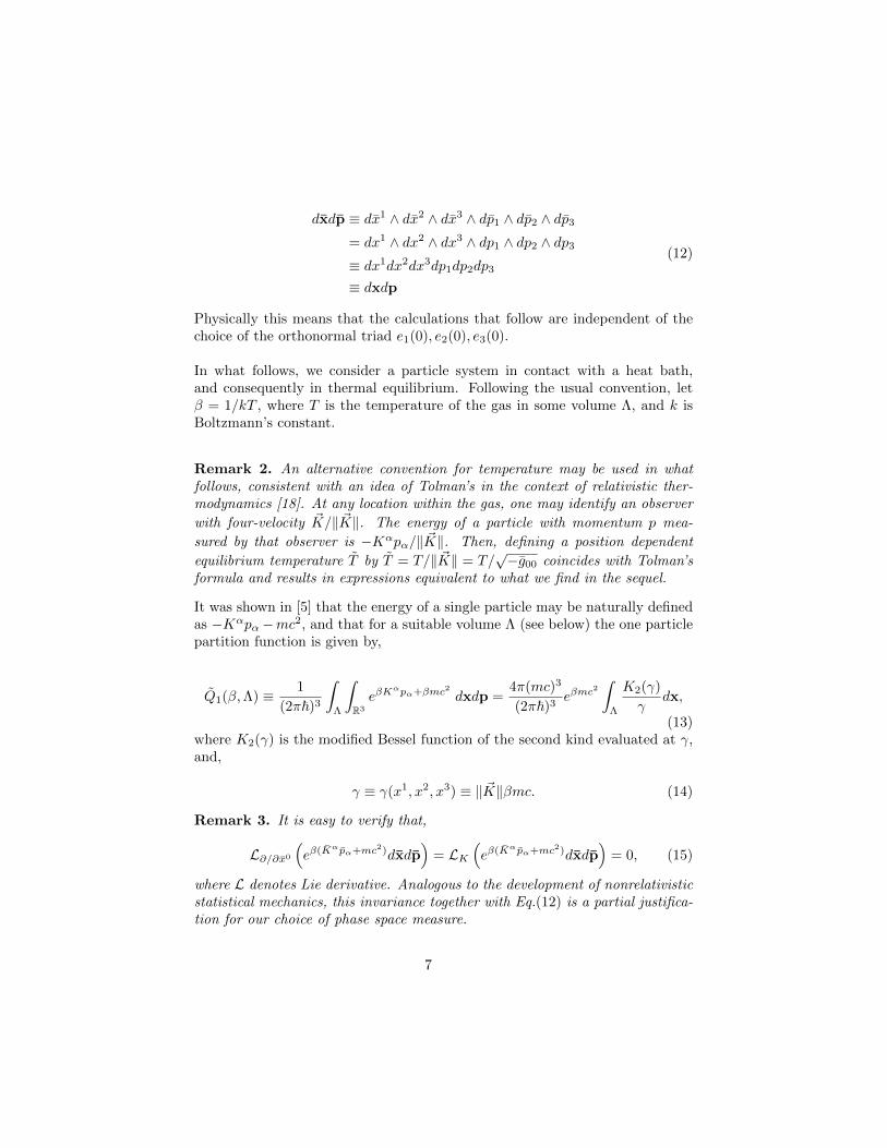
Physically this means that the calculations that follow are independent of thechoice of the orthonormal triad e1(0), e2(0), e3(0).
In what follows, we consider a particle system in contact with a heat bath,and consequently in thermal equilibrium. Following the usual convention, letβ = 1/kT , where T is the temperature of the gas in some volume Λ, and k isBoltzmann’s constant.
Remark 2. An alternative convention for temperature may be used in whatfollows, consistent with an idea of Tolman’s in the context of relativistic ther-modynamics [18]. At any location within the gas, one may identify an observer
with four-velocity ~K/‖ ~K‖. The energy of a particle with momentum p mea-
sured by that observer is −Kαpα/‖ ~K‖. Then, defining a position dependent
equilibrium temperature T by T = T/‖ ~K‖ = T/√−g00 coincides with Tolman’s
formula and results in expressions equivalent to what we find in the sequel.
It was shown in [5] that the energy of a single particle may be naturally definedas −Kαpα−mc2, and that for a suitable volume Λ (see below) the one particlepartition function is given by,
Q1(β,Λ) ≡ 1
(2π~)3
∫Λ
∫R3
eβKαpα+βmc2 dxdp =
4π(mc)3
(2π~)3eβmc
2
∫Λ
K2(γ)
γdx,
(13)where K2(γ) is the modified Bessel function of the second kind evaluated at γ,and,
γ ≡ γ(x1, x2, x3) ≡ ‖ ~K‖βmc. (14)
Remark 3. It is easy to verify that,
L∂/∂x0
(eβ(Kαpα+mc2)dxdp
)= LK
(eβ(Kαpα+mc2)dxdp
)= 0, (15)
where L denotes Lie derivative. Analogous to the development of nonrelativisticstatistical mechanics, this invariance together with Eq.(12) is a partial justifica-tion for our choice of phase space measure.
7

We take the phase space volume form for n particles to be the product of ncopies of Eq.(12), one copy for each particle, which we denote as,
dxndpn = dx11dx
21dx
31dp11dp12dp13 . . . dx
1ndx
2ndx
3ndpn1dpn2dpn3. (16)
It was shown in [5] that this measure satisfies a Liouville theorem. We now as-sume that the n-particle equilibrium distribution is determined by the followingpartition function:
Qn(β,Λ, s) ≡ enβmc2
(2π~)3n
∫Λn
∫R3n
eβ(∑ni=1 K
αpiα−VΛ(xn|s))dxndpn
=
[4π(mc)3eβmc
2
(2π~)3
]n ∫Λne−βVΛ(xn|s)
(n∏i=1
K2(γi)
γi
)dxn
(17)
where s denotes a configuration of particles outside of Λ that influences theequilibrium configuration of particles xn in Λ (s can be the empty configura-tion), VΛ(xn|s) ≡ VΛ(x1
1, x21, x
31, . . . x
1n, x
2n, x
3n|s) is a many body potential energy
function whose form and restrictions are given in the following section, andγi ≡ γ(x1
i , x2i , x
3i ). We note that this assumption excludes interaction functions
of both position and momentum coordinates, a significant restriction. However,a similar assumption for the case of special relativity was made in [19]. We em-phasize that we are not asserting that potential energy functions determine (viaa Hamiltonian) the dynamics of general relativistic particle systems; instead, weassume only that equilibrium behavior is governed by expressions of the formof Eq.(17).
3. Grand canonical ensemble on the Fermi space slice
Because the integrals in Eq.(17) factor as a product of configuration integralsand momentum integrals (which can be evaluated explicity), we focus on theformer. To proceed further, it is convenient to work with the grand canonicalensemble. A grand canonical formalism for particle systems on Riemannianmanifolds is described in [1, 2, 3] and references therein, briefly summarizedhere in way that is useful for our purposes.
Let B(X) denote the σ-algebra of Borel sets on X and Bc(X) represent thecollection of sets in B(X) with compact closure. Let ΓX be the set of particleconfigurations on X, i.e.,
ΓX = x ⊂ X : |x ∩K| <∞ for any compact K ⊂ X, (18)
8
where |A| denotes cardinality of the set A. For Λ ∈ Bc(X), define NΛ : ΓX →N0, the set of natural numbers (including zero) by,
NΛ(x) = |x ∩ Λ|. (19)
Let B(ΓX) be the σ-algebra generated by all such functions. For Λ ⊂ X, letxΛ = x ∩ Λ and,
ΓΛ = x ∈ ΓX : xX/Λ = ∅. (20)
For n = 0, 1, 2, ..., let,
Γ(n)Λ = x ∈ ΓΛ : |x| = n. (21)
There is a natural bijection,
Λn/Sn → Γ(n)Λ , (22)
where Sn is the permutation group over 1, ..., n and,
Λn ≡ (x1, ..., xn) ∈ Λn : xi 6= xj if i 6= j. (23)
If Λ ∈ Bc(X) is open, this correspondence determines a locally compact, metriz-
able topology on Γ(n)Λ and then,
ΓΛ =
∞⋃n=0
Γ(n)Λ (24)
is equipped with the topology of disjoint union and hence a Borel σ-algebra,B(ΓΛ). Then (ΓX ,B(ΓX)) is the projective limit of the measurable spaces(ΓΛ,B(ΓΛ)) as Λ increases to X, [1].
For Λ ∈ Bc(X), let BΛ = σNΛ′ : Λ′ ⊂ Λ, Λ′ ∈ Bc(X). The σ-algebras B(ΓΛ)and BΛ are σ-isomorphic.
Definition 1. Let Λ ∈ Bc(X). A set A ∈ BΛ ⊂ B(ΓX) is called a cylinder set.
Remark 4. If A is a cylinder set, let AΛ = xΛ : x ∈ A. Then 1A(x) =1AΛ(xΛ). To see this, let C = A ⊂ ΓX : 1A(x) = 1A(xΛ∪sX/Λ) for all s ∈ ΓX.Then 1A(x) = 1AΛ
(xΛ) holds if and only if A ∈ C. Let D be the class of thesets of the form x : NΛ1
(x) = n1, NΛ2(x) = n2, ..., NΛk(x) = nk, for some
nonnegative integers k, n1, n2, ..., nk, and Λ1,Λ2, ...,Λk ⊂ Λ. Then D is closedunder intersection and D ⊂ C. Moreover, C has the following properties (i)ΓX ∈ C, (ii) if A,B ∈ C and A ⊂ B then B/A ∈ C and (iii) if An ∈ Cand An ↑ A, then A ∈ C. By Dynkin’s Monotone Class Theorem, C containsσ(D) = BΛ.
9
We next define a Poisson measure on X, based on the measure dx, determined
by Eq.(12). Let Λ ∈ Bc(X) be open and let snΛ : Λn → Γ(n)Λ by snΛ((x1, ..., xn)) =
x1, ..., xn. Then dxn (snΛ)−1 is a measure on Γ(n)Λ which we again denote by
dxn (distinguished from Eq.(16) by context). For the case n = 0, dx0(∅) ≡ 1.For nonnegative activity z, and Λ ∈ Bc(X), we can define (un normalized)Poisson measure on ΓΛ by,
νΛ(dx) =
∞∑n=0
zn
n!dxn. (25)
For each Λ ∈ Bc(X), let VΛ be a B(ΓΛ) measurable interaction potential of theform,
VΛ(x) =
|x|∑n=0
∑y⊂x,|y|=n
φn(y), (26)
for finite configuration x, where φn : Γ(n)Λ → R ∪ +∞, infn,y φ(y) > −∞. For
the case n = 0, we define φ0(∅) = VΛ(∅) = |Λ|ρvac, where |Λ| is the volume ofΛ determined by the Riemannian metric 3g on X and ρvac is the energy densityof the vacuum given by
ρvac =λc4
8πG, (27)
where λ is the cosmological constant (possibly zero) and G is Newton’s universalgravitational constant.
Definition 2. An interaction potential of the form given by Eq.(26) has finiterange if for each n ≥ 2, there exists R > 0 such that φn(x1, ..., xn) = 0 wheneverthe proper distance (as determined by the Riemannian metric 3g) from xi to xjexceeds R for some i and j.
Though not essential, we assume henceforth that each φn has finite range forn > 3, so that only the two-body interactions might have infinite range. Inorder to develop notational consistency with Eq.(17), we also define a tempera-ture dependent, one-body potential (or equivalently, a temperature independentexternal field) by,
e−βφ1(x1,x2,x3) =K2(γ(x1, x2, x3))
γ(x1, x2, x3). (28)
For configurations x ⊂ Λ and s ⊂ X define,
10
VΛ(x|s) = |Λ|ρvac +
∞∑n=1
∑y⊂x∪(s∩X/Λ)
y∩x 6=∅|y|=n
φn(y), (29)
if the right hand side converges absolutely, and +∞ otherwise. For Λ ∈ Bc(X)and a boundary configuration s, define the partition function by,
ZΛ(s) = ZΛ(s, β, z) =
∫ΓΛ
e−βVΛ(x|s)νΛ(dx), (30)
where we assume that a factor 4π(mc)3eβmc2
/(2π~)3 is included in the activityz through Eq.(25) so that,
z =4π(mc)3
(2π~)3eβ(mc2+µ), (31)
where the parameter µ is chemical potential. With this identification, Eq.(30)may be rewritten as,
ZΛ(s, β, z) =
∞∑n=0
zn
n!Qn(β,Λ, s), (32)
where Q0(β,Λ, s) = exp(−β|Λ|ρvac) and for n ≥ 1,
Qn(β,Λ, s) =
∫Λne−βVΛ(x|s)dxn. (33)
Following the grand canonical statistical mechanical prescription, the connectionto thermodynamics is given by the following definitions.
Definition 3. The finite volume pressure PΛ(β, z) for Λ ∈ Bc(X) is given by,
βPΛ(β, z) =logZΛ(∅)
|Λ|, (34)
where the volume |Λ| determined by the Riemannian metric 3g on X.
Definition 4. For the case that X is unbounded, we define the infinite volumepressure P = P (β, z) by,
βP (β, z) = limn→∞
logZΛn(∅)
|Λn|, (35)
provided the limit exists. Here Λn is the ball of radius n centered at the originof Fermi-Walker-Killing coordinates.
11
Following [3], Eqs.(25) – (30) determine a local specification Π. For any s ∈ ΓX ,Λ ∈ Bc(X), and A ∈ B(X), let,
ΠΛ(A, s) =1ZΛ(s)<∞(s)
ZΛ(s)
∫ΓΛ
1A(x ∪ sX/Λ)e−βVΛ(x|s)νΛ(dx). (36)
We define a Gibbs state via the DLR equations [3].
Definition 5. Assume that X is unbounded. A probability measure µ on(ΓX ,B(ΓX)) is a Gibbs state if∫
ΓX
ΠΛ(A, s)µ(ds) = µ(A)
for all A ∈ B(ΓX) and Λ ∈ Bc(X).
Remark 5. For the case of pair potentials, conditions have been given for theexistence of Gibbs states in [3]; see also [4]. Note also that the specification givenby Eq.(36), and hence any Gibbs state, is invariant under changes of nonzeroenergy density of the vacuum φ0 (see Eq.(27)). However, the pressure is not.
4. Ideal Gas Laws
In the context of general relativity, we define an ideal gas to be the ensembledetermined by a potential V satisfying φn ≡ 0 for all n ≥ 2. Note, however,that φ1 6= 0 (see Eq.(28)), and φ0, which is proportional to the vacuum energygiven by Eq.(27), is not necessarily zero. Using the definitions of the precedingsections, a derivation of a finite volume general relativistic ideal gas law foran observer following a path tangent to a timelike Killing vector, using thegrandcanoncial ensemble is straightforward. By Def. 3,
PΛ(β, z) = −ρvac +z
β|Λ|
∫Λ
K2(γ(x))
γ(x)dx. (37)
The expected number of particles, 〈NΛ〉, in Λ is given by,
〈NΛ〉 =1
ZΛ(∅)
∞∑n=0
nzn
n!Qn(β,Λ,∅) = z
∂
∂zlogZΛ(∅) = z
∫Λ
K2(γ(x))
γ(x)dx.
(38)Combining Eqs. (37) and (38) then yields,
PΛ = −ρvac +〈NΛ〉|Λ|
kT = −ρvac + ρΛkT, (39)
where ρΛ is the number density of particles in Λ. In the case that ρvac = 0, thisis the standard form of the ideal gas law, with the volume |Λ| determined by the
12
induced metric 3g on the Fermi surface for the observer. The result is well-knownfor the case of Minkowski space-time. As in the classical (Newtonian) case, itis easily shown (using Eq.(38)) that the particle number is Poisson distributed.Thus, if PrΛ(N) represents the probability that N particles are in Λ, then,
PrΛ(N) = e−〈NΛ〉 〈NΛ〉N
N !. (40)
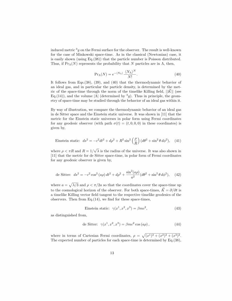
It follows from Eqs.(38), (39), and (40) that the thermodynamic behavior ofan ideal gas, and in particular the particle density, is determined by the met-ric of the space-time through the norm of the timelike Killing field, || ~K|| (seeEq.(14)), and the volume |Λ| (determined by 3g). Thus in principle, the geom-etry of space-time may be studied through the behavior of an ideal gas within it.
By way of illustration, we compare the thermodynamic behavior of an ideal gasin de Sitter space and the Einstein static universe. It was shown in [11] that themetric for the Einstein static universes in polar form using Fermi coordinatesfor any geodesic observer (with path σ(t) = (t, 0, 0, 0) in these coordinates) isgiven by,
Einstein static: ds2 = −c2dt2 + dρ2 +R2 sin2( ρR
)(dθ2 + sin2 θ dφ2), (41)
where ρ < πR and R = 1/√λ is the radius of the universe. It was also shown in
[11] that the metric for de Sitter space-time, in polar form of Fermi coordinatesfor any geodesic observer is given by,
de Sitter: ds2 = −c2 cos2 (aρ) dt2 + dρ2 +sin2(aρ)
a2(dθ2 + sin2 θ dφ2), (42)
where a =√λ/3 and ρ < π/2a so that the coordinates cover the space-time up
to the cosmological horizon of the observer. For both space-times, ~K = ∂/∂t isa timelike Killing vector field tangent to the respective timelike geodesics of theobservers. Then from Eq.(14), we find for these space-times,
Einstein static: γ(x1, x2, x3) = βmc2, (43)
as distinguished from,
de Sitter: γ(x1, x2, x3) = βmc2 cos (aρ) , (44)
where in terms of Cartesian Fermi coordinates, ρ =√
(x1)2 + (x2)2 + (x3)2.The expected number of particles for each space-time is determined by Eq.(38),
13
and respective volumes are calculated from Eqs.(41) and (42) after setting dt =0. For volumes determined by a given set of Fermi coordinates for the twospace-times, Eq.(39) and (27) yield,
PΛ = P = − λc4
8πG+ ρmass
kT
m, (45)
where ρmass = mρΛ is the mass density of the ideal gas when m is the massof each gas particle, and these densities for the two space-times depend on therespective values of γ, and will in general be different. So the relativistic ther-modynamic behavior of an ideal gas distinguishes the two space-times for anycommon value of λ.
Remark 6. It is interesting to note that the equation of state for the perfectfluid of the Einstein static universe is P = 0, with zero temperature, i.e., thefluid is “dust,” and the mass density ρ determined by the Einstein field equationsis,
ρ =λc2
4πG. (46)
If we set ρmass for the ideal gas of test particles equal to ρ of the perfect fluidand require P = 0, the temperature is given by,
kT =mc2
2, (47)
and approaches zero only as m → 0. Thus, the thermodynamic behavior of theideal gas models that of the perfect fluid (i.e. dust) only in the limiting case thatmass of each test particle of the gas goes to zero.
5. Newtonian limits
For a timelike path σ tangent to a Killing vector ~K in a given space-time, wehave defined through Eqs.(37) – (40) the relativistic grand canonical pressureof an ideal gas. Under appropriate conditions, there is associated with sucha statistical mechanical system an analogous Newtonian (i.e., nonrelativistic)expression for the pressure of the gas. It should be noted that the term “idealgas” is somewhat misleading in the context of general relativity. This is be-cause a volume of gas subject to no forces is still affected by the curvature ofspace-time, and this corresponds to a Newtonian gas subject to gravitational,tidal, and in some instances “centrifugal forces,” depending on the path of theobserver. This associated Newtonian partition function and finite volume Gibbsstate for an ideal gas is obtained as a limit as c→∞.
14
Definition 6. For a timelike Killing field ~K tangent to the path σ parameterizedby proper time τ , define a dimensionless function of the space coordinates onthe Fermi surface, α = α(x1, x2, x3), by ‖ ~K‖ = αc.
Throughout this section we let, y = 1/c so that the Newtonian limit is obtainedas y → 0+, and we assume that α can be extended to a smooth function ofy, x1, x2, x3 including at y = 0 (here and below we suppress the dependenceof α on x1, x2, x3). We refer to this function as α(y) and further assume thatα(0) = 1 and α′(0) = 0 (see the following section). Then,
α(y) = 1 +α′′(0)
2y2 +
α′′′(y0)
6y3 = 1 +
1
2α′′(0)y2 +O(y3), (48)
where 0 < y0 < y. Note that α′′(0) is a function of x1, x2, x3. Below we will iden-tify 1
2mα′′(0) as the Newtonian, nonrelativistic potential energy U(x1, x2, x3) of
a test particle of mass m with coordinates (0, x1, x2, x3) due to the gravitationalfield. This potential energy function U(x1, x2, x3) is normalized (by an addi-tive constant) so that U(0, 0, 0) = 0, i.e., the potential energy on the timelike
path σ is zero. This is because ~K is the four velocity on σ so α(y) = ‖ ~K‖/c isidentically 1 as a function of y = 1/c on σ, forcing α′′(0) = 0 there.
Definition 7. Let Λ ∈ Bc(X). For a particle system following a timelike pathσ, we define the following Newtonian statistical mechanical analogs.
(a) The Newtonian activity paramater, zNewt is given by,
zNewt =
(m
2π~2β
) 32
eβµ, (49)
where µ is the chemical potential (as in Eq.(31)).
(b) ZNewt(Λ) denotes the partition function for a non relativistic ideal gassubject to an external field with potential energy function 1
2mα′′(0) and
activity zNewt so that,
ZNewt(Λ) =
∞∑n=0
znNewt
n!
[∫Λ
e−12βmα
′′(0) dx
]n= exp
[zNewt
∫Λ
e−12βmα
′′(0) dx
] (50)
(c) Let ΠNewtΛ (A, s) denote the specification associated with the one-body New-
tonian potential 12βmα
′′(0) and partition function ZNewt(Λ) given by Eq.(36).
15
Theorem 1. Let σ be a timelike path with α satisfying Eq.(48). Assume thatΛ ∈ Bc(X). Then
(a) If ZΛ is the partition function for an ideal gas for an observer in a space-time with ρvac = 0 (i.e. with zero cosmological constant), then,
limc→∞
ZΛ = ZNewt(Λ), (51)
where as above c is the speed of light.
(b) If A ∈ BΛ then,
limc→∞
ΠΛ(A, s) = ΠNewtΛ (A, s) (52)
(where both sides of the equation are independent of s).
Proof. a) The asymptotic behavior of K2(γ) for large argument is given by (see[20]),
e−βφ1 =K2(γ)
γ∼√
π
2γ3e−γ . (53)
Since ~K is timelike, ‖ ~K‖ is nonzero and bounded below on Λ. It follows that
γ = ‖ ~K‖βmc → ∞ uniformly on Λ as c → ∞. By (53), given any ε > 0, thereexists δ > 0 such that 1/c = y < δ implies,∣∣∣∣∣∣ e−βφ1√
π2γ3 e−γ
− 1
∣∣∣∣∣∣ < ε. (54)
Multiplying by z, substituting Eqs.(31), (49), and γ = αβmc2, and rearrangingterms yields, ∣∣∣∣∣ze−βφ1 − zNewt
eβmc2(1−α)
α3/2
∣∣∣∣∣ < εzNewteβmc
2(1−α)
α3/2. (55)
Since α is smooth and the closure of Λ is compact, it follows from Eq.(48) thatα → 1 and βmc2(1 − α) → −βmα′′(0)/2, both uniformly on Λ as y → 0. Itthen follows from Eq.(55) and the triangle inequality that,
ze−βφ1 → zNewte− 1
2βmα′′(0), (56)
uniformly on Λ as y → 0. Integrating both sides of Eq.(56) then gives,
limc→∞
zQ1 = zNewt
∫Λ
e−12βmα
′′(0) dx. (57)
16
Thus,
limc→∞
ZΛ = limc→∞
exp[zQ1] = exp
[zNewt
∫Λ
e−12βmα
′′(0) dx
]= ZNewt(Λ). (58)
b) Let A ∈ BΛ be a cylinder set, and let AΛ = xΛ : x ∈ A. By Remark 4,
1A(x) = 1AΛ(xΛ). (59)
Since AΛ ⊂ ΓΛ we may write AΛ = ∪∞n=0AnΛ, where AnΛ = AΛ∩Γ
(n)Λ . From Eqs.
(25) and (36),
ΠΛ(1A, s) =1
ZΛ
∞∑n=0
1
n!
∫Λn
1AnΛ(x1, ..., xn)n∏i=1
(ze−βφ1(xi)
)dxn. (60)
By Eq.(56), there exists c0 independent of (x1, x2, x3) such that
ze−βφ1 ≤ zNewte− 1
2βmα′′(0) + 1, (61)
for all c ≥ c0 and all (x1, x2, x3) ∈ Λ. Since α′′(0) is bounded on Λ, there is aconstant C such that
∞∑n=0
1
n!
∫Λn
1AnΛ(x1, ..., xn)
n∏i=1
(zNewte
− 12βmα
′′(0) + 1)dxn
≤∞∑n=0
1
n!
∫Λn
1AnΛ(x1, ..., xn)Cndxn ≤ eC∫Λ
1dx <∞.(62)
Therefore part (b) follows from the Dominated Convergence Theorem and Eq.(58).
Corollary 1. Assume that the Fermi surface X is unbounded and let µ be theunique Gibbs state for the ideal gas. Let µNewt be the unique Newtonian Gibbsstate for the specification ΠNewt
Λ . Then for any cylinder set A,
limc→∞
µ(A) = µNewt(A). (63)
Proof. Existence and uniqueness of the Gibbs state for an ideal gas follows fromKolmogorov’s theorem for projective limit spaces (see e.g. [3] p. 21 or [21] ChapV, Theorem 3.2). Since A is a cylinder set, there exists Λ ∈ Bc(X) such thatΠΛ(A, s) is independent of s. It follows from Eq.(5) and Theorem 1 that,
limc→∞
µ(A) = limc→∞
ΠΛ(A, s) = limc→∞
ΠNewtΛ (A, s) = µNewt(A). (64)
17
Definition 8. Let PΛ(β, z), given by Eq.(37), be the pressure of an ideal gasaccording to a timelike observer satisfying the hypotheses of Theorem 1a. Wedefine the associated Newtonian pressure PNewt(β, z,Λ) to be,
βPNewt(β, z,Λ) =
(∫Λ
1 dx
)−1
logZNewt(Λ). (65)
In the case that ρvac 6= 0, we define the associated Newtonian pressure by,
βPNewt(β, z,Λ) = −ρvac +
(∫Λ
1 dx
)−1
logZNewt(Λ). (66)
We note that in the preceding definition, the role of volume Λ is restricted solelyto the identification of (constant) limits of integration for the volume integral.In the relativistic context, these limits of integration are determined by properlengths of the dimensions of the container of gas, and in the Newtonian limitthe limits of integration are absolute length measurements.
Our inclusion of the vacuum energy density term in Eq.(66) is motivated inpart by generalized Buchdahl inequalities that establish a minimum density ofmatter in space-times with a positive cosmological constant [22]. Evidently, acollection of particles falling below a certain critical density will be pushed apartby a positive vacuum energy.
6. Kerr space-time
In this section we calculate α(y) and the limiting Newtonian potential energyfunction, U(x1, x2, x3) ≡ mα′′(0)/2 for the case of circular geodesic orbit inthe equatorial plane of Kerr space-time. The Kerr metric in Boyer-Lindquistcoordinates is given by (recall that y = 1/c),
ds2 =−(
1− 2y2GMr
ρ2
)1
y2dt2 − 4y2GMar sin2 θ
ρ2dtdφ+
Σ
ρ2sin2 θdφ2
+ρ2
∆dr2 + ρ2dθ2,
(67)
where,
ρ2 = r2 + y2a2 cos2 θ,
∆ = r2 − 2GMy2r + y2a2,
Σ =(r2 + y2a2
)2 − y2a2∆ sin2 θ,
(68)
18
and where G is the gravitational constant, M is mass, and a is the angularmomentum per unit mass, and −GMy 6 a 6 GMy.
Below we will need notation for ∆, and Σ, evaluated at the specific coordinatesr = r0, and θ = π/2. For that purpose, we define,
∆0 = r20 − 2GMy2r0 + y2a2,
Σ0 =(r20 + y2a2
)2 − y2a2∆0.(69)
The circular orbit in the equatorial plane (see, e.g., [23], [24]) with dφ/dt > 0at radial coordinate r0, is given by,
σ(t) =
t, r0, π/2,t
y2a+
√r30
GM
, (70)
When a > 0, this orbit is co-rotational and when a < 0 the orbit is retrograde.All circular orbits in the equatorial plane are stable for r0 > 9GMy2, indepen-dent of a, but the co-rotational circular orbit is stable for smaller values, eveninside the ergosphere at r0 = 2GMy2 when a is sufficiently close to GMy2 (cf.[23]).
The Killing field tangent to the path (where it is the four velocity) is given by,
~K =
(y2a√GM + r
(3/2)0
D, 0, 0,
√GM
D
), (71)
where,
D =
√2y2a
√GMr
(3/2)0 + r3
0 − 3y2GMr20. (72)
Using Eqs.(67) and (71), α(y) = y√−KαKα may be found in Boyer-Lindquist
coordinates. Straightforward calculations show that α(0) = 1 and α′(0) = 0and,
1
2mα′′(0) = −GMm
r− GMmr2 sin2 θ
2r30
+3GMm
2r0. (73)
This expression may be interpreted as Newtonian potential energy of a singleparticle in a container of particles in circular orbit with angular velocity,
φ ≡ dφ
dt=
√GM
r30
, (74)
19

where r0 is the radius of the orbit. The first term on the right hand side ofEq.(73) is the gravitational potential energy, and the third term is an additiveconstant that forces α′′(0) = 0 when r = r0 and θ = π/2, i.e., at the origin ofcoordinates for the rotating container. The second term is the centrifugal poten-tial energy, more readily recognized when expressed in cylindrical coordinates.To that end, let ρ = r sin θ, with φ the azimuthal angle, and let z measure lineardistance along the axis of rotation. The magnitude of angular momentum ofa uniformly rotating particle of mass m with cylindrical coordinates (ρ, φ, z) is` = mρ2φ, and the centrifugal potential energy is then given by,
− `2
2mρ2= −GMmρ2
2r20
= −GMmr2 sin2 θ
2r30
. (75)
The minus signs in Eq.(75) take into account the direction of force, away fromthe central mass.
In order to compute α′′(0) in Fermi coordinates, we select the following tetradvectors in the tangent space at σ(0).
e0 =
(y2a√GM + r
(3/2)0
D, 0, 0,
√GM
D
),
e1 =
(0,
√∆0
r0, 0, 0
),
e2 =
(0, 0,
1
r0, 0
), (76)
e3 =
(y2√GM
(y2a2+r2
0−2y2a√GMr0
)D√
∆0
, 0, 0,y2√GM(a− 2
√r0) + r
(3/2)0
D√
∆0
)
This tetrad may be extended via parallel transport to the entire circular orbitgiven by Eq.(70), but we need these tetrad vectors only at σ(0).
Fermi coordinates relative to these coordinate axes (i.e., the above tetrad) maybe calculated using Eq.(27) of [13]. The result for the Boyer-Lindquist coordi-nates r and θ to second order expressed in the Fermi space coordinates x1, x2, x3
20

at (x0 = τ = t = 0) is,
θ =π
2+x2
r0−√
∆0 x1x2
r30
+ · · · , (77)
r = r0 +
√∆0 x
1
r0+
(r0y
2GM − y2a2) (x1)2
2r30
+∆0
(x2)2
2r30
+
(r0 − y2GM
) (x3)2
2r20
+ · · · , (78)
Now, calculating α(y) = y√−KαKα in Boyer-Lindquist coordinates, substitut-
ing for r and θ using Eqs.(77) and (78) gives,
α(y) = 1 +GMy2
(r20 + 3 a2y2 − 4 ay2
√r0GM
) (x2)2
2 r20 D2
−3GMy2∆0
(x1)2
2 r20 D2
+O(3)
(79)
Computing the second derivative with respect to y at y = 0 yields,
1
2mα′′(0) =
−GMm
r0+GMmx1
r20
−GMm
(2(x1)2 − (x2
)2 − (x3)2)
2r30
−
GMm
2r0+GMmx1
r20
+GMm
((x1)2
+(x3)2)
2r30
+3GMm
2r0+O(3).
(80)
Eq.(80) may be compared term-by-term with Eq.(73). The expression in thefirst pair of parentheses on the right hand side of Eq.(80) is the Taylor expan-sion to second order of the gravitational potential, which is the first term onthe right hand side of Eq.(73). The second terms in both equations are relatedanalogously. At the point σ(0) in the orbit, the Cartesian variable x1 in Eq.(80)measures (Newtonian) distance from the origin of coordinates in the radial di-rection away from the central mass, x2 measures distance in the “z direction”parallel to the axis of rotation, and x3 measures distance in the tangential di-rection, parallel to the motion of the container of gas in orbit. (However, theseorientations do not hold at other parts of the orbit since the coordinate axes arenonrotating.) Eq.(80) may obviously be simplified to yield the potential energyfunction,
21
U(x1, x2, x3) =1
2mα′′(0) = −
3GmM(x1)2
2r30
+GmM
(x2)2
2r30
+O(3). (81)
Combining Eq.(81) with Eqs.(50) and (65) immediately yields the Newtonianpressure (with y = 1/c) for a gas in circular orbit around a central mass towhich the relativistic counterpart given by Eq.(37) may be compared.
7. Anti-de Sitter space
In this section, we prove uniqueness of the infinite volume Gibbs state in anti-deSitter space for a class of equilibrium interaction potentials and calculate theinfinite volume relativistic pressure for an ideal gas of test particles.
Explicit transformation formulas to and from Fermi coordinates x0, x1, x2, x3for a geodesic observer in (the covering space for) anti-de Sitter space-time aregiven in [11]. The geodesic path of the Fermi observer in these coordinates isσ(t) = (t, 0, 0, 0). Fermi coordinates for this space-time are global, i.e., one co-ordinate patch covers the entire space-time.
Under the change of coordinates, x0 = t, x1 = ρ sin θ cosφ, x2 = ρ sin θ sinφ,x3 = ρ cos θ, the metric becomes diagonal. In these “polar-Fermi coordinates,”for any appropriate range of the angular coordinates, the line element becomes,
ds2 = −c2 cosh2 (aρ) dt2 + dρ2 +sinh2(aρ)
a2(dθ2 + sin2 θ dφ2), (82)
where a =√|λ|/3 and λ < 0 is the cosmological constant. For this space-time,
~K = ∂/∂t is a timelike Killing vector field tangent to σ so that e0 = ~K. FromEqs.(14) and (82),
γ(x1, x2, x3) = ‖ ~K‖βmc = βmc2 cosh(aρ), (83)
where ρ =√
(x1)2 + (x2)2 + (x3)2. The Fermi surface, X, given by Eq.(8), ishyperbolic space.
Because a single chart, with domain R3, covers the entire Fermi surface for thisspace-time, each configuration of particles on the Fermi surface corresponds toa configuration on R3, and Gibbs states on the Fermi surface are in a naturalone-to-one correspondence with Gibbs states of configurations on R3 with Pois-son measure of Eq.(25) based on Lebesgue measure dx. For an elaboration, see[1, 2, 3]. In this context, and noting Remark 5, we may regard V as an interac-tion on configurations on R3 and apply the following special case of Theorem 1
22
of [25] to the present circumstances.
Theorem 2. Suppose there exists an increasing sequence of bounded Borel setsΛk whose union is R3 such that:
(1) φn(x) = 0, for any n ≥ 2 and x = (x1, ..., xn) such that x ∩ Λk 6= ∅ 6=x ∩ (R3/Λk+1) for some k;
(2)∑k [sups ZAk(s, β, z)]
−1diverges, where Ak = Λk+1/Λk.
Then there is at most one Gibbs state for V, β, z.
Assume that V is a superstable interaction and has the form given by Eqs.(28)and (29). Assume further that V has finite range and satisfies the condition,
VΛ(x1, ..., xn|s) ≡∞∑n=2
∑y⊂x∪(s∩X/Λ)
y∩x 6=∅|y|=n
φn(y) > −Bn, (84)
for some B > 0, all boundary configurations s, and all configurations (x1, ..., xn).Observe that V is the same as V except that V does not include the vacuumenergy φ0 or the one-body potential function, φ1. The potential V satisfiesEq.(84) if it is positive or satisfies a hard-core condition (see [25]).
Theorem 3. Let V be a potential energy function with finite range R satisfyingEq.(84) on the Fermi surface X in anti-de Sitter space. Then there is at mostone Gibbs state on (ΓX ,B(ΓX)) for V, β, z for all choices of β and z.
Proof. Let Λk ⊂ X be the sphere of radius kR centered at the origin of coordi-nates in the chart for X, where R is as in Def. 2. Then condition (1) of Theorem2 is satisfied by Λk. To see that condition (2) of Theorem 2 is also satisfied,let Ak be defined as in Theorem 2 and observe by Eq.(84) that,
supsZAk(s, β, z) ≤
∫ΓAk
exp
βBn− β |x|∑i=1
φ1(xi)
νAk(dx). (85)
It follows from Eqs.(53) and (83) that when ρ =√
(x1)2 + (x2)2 + (x3)2 issufficiently large,
e−βφ1(x1,x2,x3) ≤ e−βmc2 cosh(aρ). (86)
Then for large k,
23
supsZAk(s, β, z) ≤
∞∑n=0
exp[βBn− βn cosh(kR)]zn
n!|Ak|n, (87)
where |Ak| =∫Akdx1dx2dx3, i.e., the Lebesgue measure of the image of Ak in
the Fermi coordinate chart. Hence, |Ak| < C(kR)2 for a constant C. Thus,
supsZAk(s, β, z) ≤ exp[zC(Rk)2eβB−β cosh(kR)], (88)
and condition (2) of Theorem 2 is clearly satisfied.
Corollary 2. The pressure of an ideal gas of test particles in anti-de Sitterspace is given by,
P = − λc4
8πG, (89)
where λ < 0 is the cosmological constant for anti-de Sitter space.
Proof. With the same notation as in the proof of Theorem 3, using Eq.(37) andchanging to spherical coordinates, we find,
PΛk(β, z) = −ρvac +4πz
βmc2|Λk|
∫ k
0
K2(βmc2 cosh(aρ))
cosh(aρ)ρ2dρ. (90)
The result now follows from Eqs.(35), (27), and (53).
Remark 7. The infinite volume pressure of an ideal gas of test particles in anti-de Sitter space is independent of temperature and chemical activity, and dependsonly on the magnitude of the cosmological constant. There is no correspondingNewtonian analog, as developed in Sect. 5, because Eq.(48) does not hold forthe Killing vector ∂/∂t.
8. Concluding Remarks
For space-times with timelike Killing fields, we have developed a grand canonicalformalism for statistical mechanical systems of test particles. The thermody-namic behavior of an ideal gas was shown in Sect. 4 to be determined by themetric of the space-time through the norm of the timelike Killing field, and thevolume of the particle system as determined by projection 3g of the metric onthe Fermi space slice of the timelike observer.
We proved uniqueness of the Gibbs state for a class of interaction potentials inanti-de Sitter space, and found the infinite volume pressure for an ideal gas oftest particles. For the case of an ideal gas in space-times where Eq.(48) is sat-isfied, we introduced a notion of Newtonian limit of Gibbs states and of grand
24

canonical pressures. The physical legitimacy of the grand canonical formalismwas demonstrated in Sect. 6, where it was shown that the Newtonian limit of arelativistic particle system following a circular geodesic orbit in Kerr space-timeresults in exactly what is predicted by classical mechanics.
Directions for further research include possible generalizations of the statisticalmechanical formalism which assume only the existence of approximate timelikeKilling vector fields or conformal timelike Killing fields, relaxing our assumptionof the existence of a timelike Killing vector field. In addition, alternative notionsof simultaneity associated with coordinate systems other than Fermi-Walker-Killing coordinates might be considered, such as standard curvature-normalizedcoordinates on Robertson-Walker cosmologies for observers co-moving with theHubble flow, or optical coordinates (in which events are “simultaneous” if theyare visible to the observer σ at the same proper time coordinate of σ). In thisway, the effect of the curvature of space on statistical mechanical behavior oftest particles might be analyzed for realistic circumstances.
Acknowledgment. The authors wish to thank Peter Collas for helpful discus-sions.
References
[1] Rockner, M.: Stochastic analysis on configuration spaces: basic ideas andrecent results arXiv:math/9803162v1 [math.PR] (1998).
[2] Albeverio, P., Kondratiev, Y., Rockner, M.: Analysis and Geometry onConfiguration Spaces: The Gibbsian Case J. Functional Analysis 157, 242-291 (1998).
[3] Kuna, T.: Studies in Configuration Space Analysis and Applications,Bonner Math. Schrift., 324, Univ. Bonn, Bonn, 1999, PhD dissertation,Rheinische Friedrich-Wilhelms-Universitat Bonn, Bonn (1999), 187 pp.MR1932768 (2003k:82058).
[4] Kondratiev, Y., Pasurek, T., Rockner, M.: Gibbs Measuresof Continuous Systems: an analytic approach www.math.uni-bielefeld.de/sfb701/preprints/sfb09019.pdf (2009).
[5] Klein, D., Collas, P.: Timelike Killing fields and relativistic statistical me-chanics, Class. Quantum Grav. 26, 045018 (16 pp) arXiv:0810.1776v2 [gr-qc] (2009).
[6] Montesinos, M., Rovelli, C.: Statistical mechanics of generally covariantquantum theories: a Boltzmann-like approach Class. Quantum Grav. 18,555-569 (2001).
25
[7] Misner, C. W., Thorne, K. S., and Wheeler, J. A. (1973). Gravitation, W.H. Freeman, San Francisco.
[8] Walker, A. G.: Note on relativistic mechanics Proc. Edin. Math. Soc. 4,170-174 (1935).
[9] Synge, J. L.: Relativity: The General Theory North Holland, Amsterdam(1960).
[10] Collas, P., Klein, D.: A Simple Criterion for Nonrotating Reference Frames,Gen. Rel. Grav. 36, 1493-1499 (2004).
[11] Klein, D., Collas, P.: Exact Fermi coordinates for a class of space-times, J. Math. Phys. 51, 022501, (10 pp) DOI:10.1063/1.3298684,arXiv:0912.2779v1 [math-ph] (2010).
[12] O’Neill, B.: Semi-Riemannian geometry with applications to relativity(1983). Academic Press, New York, p. 200.
[13] Klein, D., Collas, P., General Transformation Formulas for Fermi-WalkerCoordinates Class. Quant. Grav. 25, 145019 (17pp) DOI:10.1088/0264-9381/25/14/145019, [gr-qc] arxiv.org/abs/0712.3838v4 (2008).
[14] Bolos, V.: Intrinsic definitions of “relative velocity” in general relativityComm. Math. Phys. 273, 217-236 (2007).
[15] Klein, D., Randles, E., Fermi coordinates, simultaneity, and expandingspace in Robertson-Walker cosmologies Ann. Henri Poincare 12 303–28(2011) DOI: 10.1007/s00023-011-0080-9.
[16] Bolos, V., Klein D., Relative velocities for radial motion in expandingRobertson-Walker spacetimes Archive: arXiv:1106.3859v1 [gr-qc]
[17] Collas, P., Klein, D., A Statistical mechanical problem in Schwarzschildspace-time Gen. Rel. Grav. 39, 737-755 DOI:10.1007/s10714-007-0416-4(2007).
[18] Tolman, R. C.: Relativity, thermodynamics, and cosmology. Clarendon,Oxford (1934) pp. 318-9.
[19] Horwitz, L. P., Schieve, W. C., Piron, C.: Gibbs ensembles in relativisticclassical and quantum mechanics Ann. Phys., NY 137, 306-340 (1981).
[20] Erdelyi, A. (1953) Higher Transcendental Functions Vol. II. McGraw-Hill,New York, p. 23.
[21] Parthasarathy, K. R., Probability measures on metric spaces, Probabil-ity and mathematical statistics, Academic Press, New York and London(1967).
26
[22] Bohmer, C.G., Harko, T.: Does the cosmological constant imply the ex-istence of a minimum mass? Phys. Lett. B 630, 73-77 (2005) [arXiv:gr-qc/0509110].
[23] Bardeen, J. M., Press, W. H., Teukolsky, S. A., Rotating Black Holes:Locally Nonrotating Frames, Energy Extraction, and Scalar SynchrotronRadiation The Astrophysical Journal 178, 347-369 (1972).
[24] Bonnor, W., Steadman, B., The gravitomagnetic clock effect Class. Quant.Grav. 16, 1853–1861(1999).
[25] Klein, D., Yang, W.S.: Absence of phase transitions for continuum modelsof dimension d > 1 J. Math. Phys 29, 1130-1133 (1988).
27