graph coloring problems - departamento de matematica
TRANSCRIPT

Graph Coloring Problems
Guillermo Duran
Departamento de Ingenierıa IndustrialFacultad de Ciencias Fısicas y Matematicas
Universidad de Chile, Chile
XII ELAVIO, February 2007, Itaipava, Brasil

The Four-Color problem
StatementHistoryFirst attemptsThe proofs
The Four-Color problem
The Four-Color problem
StatementHistoryFirst attemptsThe proofs
The Four-Color problem
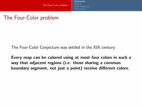
The Four-Color Conjecture was settled in the XIX century:
Every map can be colored using at most four colors in such away that adjacent regions (i.e. those sharing a commonboundary segment, not just a point) receive different colors.

The Four-Color problem
StatementHistoryFirst attemptsThe proofs
In terms of graphs...
Clearly a graph can be constructed from any map, the regionsbeing represented by the vertices of the graph and two verticesbeing joined by an edge if the regions corresponding to the verticesare adjacent.
The resulting graph is planar, that is, it can be drawn in the planewithout any edges crossing.
So, the Four-Color Conjecture asks if the vertices of a planar graphcan be colored with at most 4 colors so that no two adjacentvertices use the same color.

The Four-Color problem
StatementHistoryFirst attemptsThe proofs
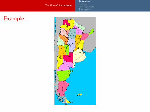
Example...
The Four-Color problem
StatementHistoryFirst attemptsThe proofs
Example...

The Four-Color problem
StatementHistoryFirst attemptsThe proofs
Example...

The Four-Color problem
StatementHistoryFirst attemptsThe proofs
History
The Four-Color Conjecture first seems to havebeen formulated by Francis Guthrie. He was astudent at University College London where hestudied under Augusts De Morgan.
After graduating from London he studied law butsome years later his brother Frederick Guthrie hadbecome a student of De Morgan. Francis Guthrieshowed his brother some results he had beentrying to prove about the coloring of maps andasked Frederick to ask De Morgan about them.
Guthrie
De Morgan

The Four-Color problem
StatementHistoryFirst attemptsThe proofs
De Morgan was unable to give an answer but, on 23 October 1852, thesame day he was asked the question, he wrote a letter to Sir WilliamHamilton in Dublin:
A student of mine asked me today to give him a reason for a fact which Idid not know was a fact - and do not yet. He says that if a figure beanyhow divided and the compartments differently colored so that figureswith any portion of common boundary line are differently colored - fourcolors may be wanted, but not more - the following is the case in whichfour colors are wanted. Query cannot a necessity for five or more beinvented. ... If you retort with some very simple case which makes meout a stupid animal, I think I must do as the Sphynx did...
Hamilton replied on 26 October 1852 (showing theefficiency of both himself and the postal service):
I am not likely to attempt your quaternion of colorsvery soon.
Hamilton

The Four-Color problem
StatementHistoryFirst attemptsThe proofs
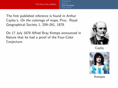
The first published reference is found in ArthurCayley’s, On the colorings of maps, Proc. RoyalGeographical Society 1, 259–261, 1879.
On 17 July 1879 Alfred Bray Kempe announced inNature that he had a proof of the Four-ColorConjecture.
Kempe was a London barrister who had studiedmathematics under Cayley at Cambridge anddevoted some of his time to mathematicsthroughout his life.
At Cayley’s suggestion Kempe submitted theTheorem to the American Journal of Mathematicswhere it was published in the ends of 1879.
Cayley
Kempes
The Four-Color problem
StatementHistoryFirst attemptsThe proofs
The first published reference is found in ArthurCayley’s, On the colorings of maps, Proc. RoyalGeographical Society 1, 259–261, 1879.
On 17 July 1879 Alfred Bray Kempe announced inNature that he had a proof of the Four-ColorConjecture.
Kempe was a London barrister who had studiedmathematics under Cayley at Cambridge anddevoted some of his time to mathematicsthroughout his life.
At Cayley’s suggestion Kempe submitted theTheorem to the American Journal of Mathematicswhere it was published in the ends of 1879.
Cayley
Kempes

The Four-Color problem
StatementHistoryFirst attemptsThe proofs
The first published reference is found in ArthurCayley’s, On the colorings of maps, Proc. RoyalGeographical Society 1, 259–261, 1879.
On 17 July 1879 Alfred Bray Kempe announced inNature that he had a proof of the Four-ColorConjecture.
Kempe was a London barrister who had studiedmathematics under Cayley at Cambridge anddevoted some of his time to mathematicsthroughout his life.
At Cayley’s suggestion Kempe submitted theTheorem to the American Journal of Mathematicswhere it was published in the ends of 1879.
Cayley
Kempe

The Four-Color problem
StatementHistoryFirst attemptsThe proofs
Idea of Kempe’s proof
Kempe used an argument known as the method ofKempe chains.
If we have a map in which every region is colored red,green, blue or yellow except one, say X. If this finalregion X is not surrounded by regions of all four colorsthere is a color left for X. Hence suppose that regionsof all four colors surround X.
If X is surrounded by regions A, B, C, D in order,colored red, yellow, green and blue then there are twocases to consider.
(i) There is no chain of adjacent regions from A to Calternately colored red and green.
(ii) There is a chain of adjacent regions from A to Calternately colored red and green.
BA C
D
X
BA C
D
X
BA C
D
X

The Four-Color problem
StatementHistoryFirst attemptsThe proofs
Cases:
(i) There is no chain of adjacent regions from A to Calternately colored red and green.
(ii) There is a chain of adjacent regions from A to Calternately colored red and green.
If (i) holds there is no problem. Change A to green,and then interchange the color of the red/greenregions in the chain joining A. Since C is not in thechain it remains green and there is now no red regionadjacent to X. Color X red.
If (ii) holds then there can be no chain of yellow/blueadjacent regions from B to D. [It could not cross thechain of red/green regions.] Hence property (i) holdsfor B and D and we change colors as above.
BA C
D
X
BA C
D
X

The Four-Color problem
StatementHistoryFirst attemptsThe proofs
Cases:
(i) There is no chain of adjacent regions from A to Calternately colored red and green.
(ii) There is a chain of adjacent regions from A to Calternately colored red and green.
If (i) holds there is no problem. Change A to green,and then interchange the color of the red/greenregions in the chain joining A. Since C is not in thechain it remains green and there is now no red regionadjacent to X. Color X red.
If (ii) holds then there can be no chain of yellow/blueadjacent regions from B to D. [It could not cross thechain of red/green regions.] Hence property (i) holdsfor B and D and we change colors as above.
X
BA C
D
X
BA C
D

The Four-Color problem
StatementHistoryFirst attemptsThe proofs
The Four-Color Theorem returned to being the Four-ColorConjecture in 1890.
Percy John Heawood, a lecturer at Durham England,published a paper called Map coloring theorem. In ithe states that his aim is “...rather destructive thanconstructive, for it will be shown that there is a defectin the now apparently recognised proof...”.
Although Heawood showed that Kempe’s proof was
wrong he did prove that every map can be 5-colored in
this paper.Heawood
Exercise
Using Kempe’s ideas, prove that every map can be 5-colored.
Hint: Every planar graph has at least one vertex of degree atmost 5.

The Four-Color problem
StatementHistoryFirst attemptsThe proofs
It was not until 1976 that the four-colorconjecture was finally proven by Kenneth Appeland Wolfgang Haken at the University of Illinois.They were assisted in some algorithmic work byJohn Koch.
K. Appel and W. Haken, Every planar map isfour colorable. Part I. Discharging, Illinois J.Math. 21 (1977), 429–490.
K. Appel, W. Haken and J. Koch, Everyplanar map is four colorable. Part II.Reducibility, Illinois J. Math. 21 (1977),491–567.
Appel
The Four-Color problem
StatementHistoryFirst attemptsThe proofs
Idea of the proof
If the four-color conjecture were false, there would be at least onemap with the smallest possible number of regions that requires fivecolors. The proof showed that such a minimal counterexamplecannot exist through the use of two technical concepts:
An unavoidable set contains regions such that every map musthave at least one region from this collection.
A reducible configuration is an arrangement of countries thatcannot occur in a minimal counterexample. If a map containsa reducible configuration, and the rest of the map can becolored with four colors, then the entire map can be coloredwith four colors and so this map is not minimal.
The Four-Color problem
StatementHistoryFirst attemptsThe proofs
Idea of the proof
Using different mathematical rules and procedures, Appel andHaken found an unavoidable set of reducible configurations, thusproving that a minimal counterexample to the four-color conjecturecould not exist.
Their proof reduced the infinitude of possible maps to 1,936reducible configurations (later reduced to 1,476) which had to bechecked one by one by computer.
However, the unavoidability part of the proof was over 500 pagesof hand written counter-counter-examples (these graph coloringswere verified by Haken’s son!). The computer program ran forhundreds of hours.

The Four-Color problem
StatementHistoryFirst attemptsThe proofs
But most of the researchers thought that there were two reasonswhy the Appel-Haken proof was not completely satisfactory.
Part of the Appel-Haken proof uses a computer, and cannotbe verified by hand, and
Even the part that is supposedly hand-checkable isextraordinarily complicated and tedious, and no one hasverified it in its entirety.

The Four-Color problem
StatementHistoryFirst attemptsThe proofs
Ten years ago, another proof:
N. Robertson, D. P. Sanders, P. D. Seymour and R. Thomas,The four color theorem, J. Combin. Theory Ser. B. 70(1997), 2–44.
N. Robertson, D. P. Sanders, P. D. Seymour and R. Thomas,A new proof of the four color theorem, Electron. Res.Announc. Amer. Math. Soc. 2 (1996), 17–25 (electronic).
Robertson Sanders Seymour Thomas

The Four-Color problem
StatementHistoryFirst attemptsThe proofs
Outline of the proof
The basic idea of the proof is the same as Appel and Haken’s. Theauthors exhibit a set of 633 “configurations”, and prove each ofthem is “reducible”. Recall, that this is a technical concept thatimplies that no configuration with this property can appear in aminimal counterexample to the Four-Color Theorem. It has beenknown since 1913 that every minimal counterexample to theFour-Color Theorem should be a special structure, called“internally 6-connected triangulation”.
In the second part of the proof they prove that at least one of the633 configurations appears in every internally 6-connected planartriangulation. This is called proving unavoidability, and here themethod used differs from that of Appel and Haken. The first partof proof needs a computer. The second part can be checked byhand in a few months, or, using a computer, it can be verified inabout 20 minutes.

The Four-Color problem
StatementHistoryFirst attemptsThe proofs
Why is this proof “better”?
The unavoidable set has size 633 as opposed to the 1476 memberset of Appel and Haken, and the second part of the proof uses onlyabout 30 rules, instead of the 300+ of Appel and Haken (and bycomputer can be verified in about 20 minutes against hundred ofhours of the other proof).

The Four-Color problem
StatementHistoryFirst attemptsThe proofs
At December 2004 in a scientific meeting in France, a joint groupbetween people by Microsoft Research in England and INRIA inFrance announced the verification of the Robertson et al. proof byformulating the problem in the equational logic program Coq andconfirming the validity of each of its steps (Devlin 2005,Knight 2005).

The Four-Color problem
StatementHistoryFirst attemptsThe proofs
But in both cases (Appel and Haken, and Robertson et al.), the‘proofs’ are not proofs in the traditional sense, because theycontain steps that can never be verified by humans. Up today, atraditional mathematical proof is not known for the Four-ColorTheorem.

Some basic concepts about computational complexityNP-completeness theoryP 6= NP? or P = NP?NP-completeness proofs
Some basic concepts about computationalcomplexity

Some basic concepts about computational complexityNP-completeness theoryP 6= NP? or P = NP?NP-completeness proofs
Some basic concepts about computational complexity
A problem is a general question to be answered, usuallypossessing several parameters, whose values are leftunspecified.
A problem is described by giving:
1. A general description of all its parameters.2. A statement of what properties the answer (or solution) is
required to satisfy.
The difficulty of a problem is related to its structure and thelength of the instance to be considered. This length is givenby one or two parameters, for example, in the graph coloringproblem, the number of vertices of the graph.
Some basic concepts about computational complexityNP-completeness theoryP 6= NP? or P = NP?NP-completeness proofs
Some basic concepts about computational complexity
In order to know the complexity of an algorithm we need tocalculate the number of elementary arithmetic operations thatthe algorithm does to solve a given problem. This number is afunction of the length of the instance.
We say that a problem is in P if there exists an algorithm ofpolynomial complexity to solve it (the number of thoseoperations is always upper bounded by a polynomial functionin n, the input length).

Some basic concepts about computational complexityNP-completeness theoryP 6= NP? or P = NP?NP-completeness proofs
NP-completeness theory
It is applied to decision problems, problems whose answer is“YES” or “NOT” (but it is easy to see that this theory hasseveral consequences on optimization problems).
For example, the decision problem related to the graphcoloring problem is the following: “Given a graph G and aninteger number k, is there a valid coloring with at most kcolors?”
A decision problem π consists of a set Dπ of instances and asubset Yπ ⊆ Dπ whose answer is “YES”.
Some basic concepts about computational complexityNP-completeness theoryP 6= NP? or P = NP?NP-completeness proofs
NP-completeness theory
A problem π ∈ NP if there exists a polynomial certificate toverify an instance of “YES” (this is, if I can verify inpolynomial time that an instance of “YES” is right).
So, it is not difficult to see that P ⊆ NP.
Open Conjecture: P 6= NP.

Some basic concepts about computational complexityNP-completeness theoryP 6= NP? or P = NP?NP-completeness proofs
Polynomial reduction
Let π and π′ be two decision problems. We say thatf : Dπ′ → Dπ is a polynomial reduction of π′ in π if f can becomputed in polynomial time and for every d ∈ Dπ′ ,d ∈ Yπ′ ⇔ f (d) ∈ Yπ. Notation: π′ 4 π.
Note that if π′′ 4 π′ and π′ 4 π then π′′ 4 π, because thecomposition of two polynomial reductions is a polynomialreduction.

Some basic concepts about computational complexityNP-completeness theoryP 6= NP? or P = NP?NP-completeness proofs
NP-complete problems
A problem π is NP-complete if:
1. π ∈ NP.2. For every π′ ∈ NP, π′ 4 π.
If a problem π verifies condition 2., we say that π is NP-hard(it is so “difficult” as all the problems in NP).
Some basic concepts about computational complexityNP-completeness theoryP 6= NP? or P = NP?NP-completeness proofs
P 6= NP? or P = NP?
If there is a problem π ∈ NP-c ∩ P, then P=NP.
If π ∈ NP-c ∩ P, there is a polynomial time algorithm to solveπ, because π is in P. On the other hand, as π ∈ NP-c, forevery π′ ∈ NP, π′ 4 π.
Let π′ be in NP. We have to use the polynomial reductionwhich transforms instances of π′ in instances of π, and thenthe polynomial time algorithm which solves π. It is easy to seethat we obtain a polynomial time algorithm to solve π′.
It is known any problem neither in NP-c ∩ P, nor in NP \ P(in this last case, it would be proved that P 6= NP).

Some basic concepts about computational complexityNP-completeness theoryP 6= NP? or P = NP?NP-completeness proofs
Inclusions between the classes
Some basic concepts about computational complexityNP-completeness theoryP 6= NP? or P = NP?NP-completeness proofs
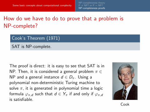
How do we have to do to prove that a problem isNP-complete?
Cook’s Theorem (1971)
SAT is NP-complete.
The proof is direct: it is easy to see that SAT is inNP. Then, it is considered a general problem π ∈NP and a general instance d ∈ Dπ. Using apolynomial non-deterministic Turing machine tosolve π, it is generated in polynomial time a logicformula ϕπ,d such that d ∈ Yπ if and only if ϕπ,d
is satisfiable.Cook

Some basic concepts about computational complexityNP-completeness theoryP 6= NP? or P = NP?NP-completeness proofs
How do we have to do to prove that a problem isNP-complete?
Using Cook’s Theorem, the standard technique to prove that aproblem π is NP-complete uses the transitivity of 4, and consistsin the following:
1. Prove that π is in NP.
2. Choose an appropriated problem π′ belonging to NP-c.
3. Build a polynomial reduction f of π′ in π.
The second condition of the definition holds using the transitivity:let π′′ be a problem in NP. As π′ is NP-c, π′′ 4 π′. But it wasproved that π′ 4 π, so π′′ 4 π.

Some basic concepts about computational complexityNP-completeness theoryP 6= NP? or P = NP?NP-completeness proofs
Some famous problems in NP-c
Traveling Salesman Problem (TSP)
Graph coloring
Integer Programming

Graph coloring
Chromatic numberGraph coloring algorithmsChromatic polynomialChromatic index
Graph coloring

Graph coloring
Chromatic numberGraph coloring algorithmsChromatic polynomialChromatic index
Graph coloring
A k-coloring of a graph G is an assignment of one color toeach vertex of G such that no more than k colors are usedand no two adjacent vertices receive the same color.
A graph is called k-colorable iff it has a k-coloring.
4-coloring 3-coloring

Graph coloring
Chromatic numberGraph coloring algorithmsChromatic polynomialChromatic index
Chromatic numberA clique in a graph G is a complete subgraph maximal underinclusion. The cardinality of a maximum clique is denoted byω(G ).The chromatic number of a graph G is the smallest number ksuch that G is k-colorable, and it is denoted by χ(G ). Anobvious lower bound for χ(G ) is ω(G ):
ω(G ) ≤ χ(G ) ∀G .
ω = 3 χ = 4
Graph coloring
Chromatic numberGraph coloring algorithmsChromatic polynomialChromatic index
Applications
The problem of coloring a graph has several applications such asscheduling, register allocation in compilers, frequency assignmentin Mobile radios, etc.
Example: Examination schedule
Each student must take an examination in each of his/her courses.Let X be the set of different courses and let Y be the set ofstudents. Since the examination is written, it is convenient that allstudents in a course take the examination at the same time. Whatis the minimum number of examination periods needed?
Exercise
Model this problem as a coloring problem.

Graph coloring
Chromatic numberGraph coloring algorithmsChromatic polynomialChromatic index
Computational complexity
The graph k-colorability problem is the following:
INSTANCE: A graph G = (V ,E ) and a positive integer k ≤ V .
QUESTION: Is G k-colorable?
This problem is NP-complete (Karp, 1972), andremains NP-c for k = 3.
Exercise
What happens for k = 2?
Karp
Graph coloring
Chromatic numberGraph coloring algorithmsChromatic polynomialChromatic index
Planar graphs coloring
For planar graphs the paper by Robertson et al. gives a quadraticalgorithm to four-color planar graphs, an improvement over thequadric algorithm by Appel and Haken.
Exercise
Does it mean that the k-colorability problem is polynomial forplanar graphs?

Graph coloring
Chromatic numberGraph coloring algorithmsChromatic polynomialChromatic index
Some easy properties about χ(G )
Let G be a graph with n vertices and G its complement.Then:
χ(G ) ≤ ∆(G ) + 1, where ∆(G ) is the maximum degree of G .
χ(G ) ω(G ) ≥ n
χ(G ) + ω(G ) ≤ n + 1
χ(G ) + χ(G ) ≤ n + 1

Graph coloring
Chromatic numberGraph coloring algorithmsChromatic polynomialChromatic index
Brooks’ Theorem
Brooks’ Theorem (1941)
Let G be a connected graph. Then G is ∆(G )-colorable, unless:
1. ∆(G ) 6= 2, and G is a ∆(G ) + 1-clique, or
2. ∆(G ) = 2, and G is an odd cycle.

Graph coloring
Chromatic numberGraph coloring algorithmsChromatic polynomialChromatic index
Graph coloring algorithms
As it was said, it is not known a polynomial time algorithm todetermine χ(G ). Let us see the following no efficient algorithm(contraction-connection):
Consider a graph G with two non-adjacent vertices a and b. Theconnection G1 is obtained by joining the two non-adjacent vertices aand b with an edge. The contraction G2 is obtained by shrinking{a, b} into a single vertex c(a, b) and by joining it to each neighborin G of vertex a and of vertex b (and eliminating multiple edges).
A coloring of G in which a and b have the same color yields acoloring of G1. A coloring of G in which a and b have differentcolors yields a coloring of G2.
Repeat the operations of connection and contraction in each graphgenerated, until the resulting graphs are all cliques. If the smallestresulting clique is a k-clique, then χ(G ) = k.

Graph coloring
Chromatic numberGraph coloring algorithmsChromatic polynomialChromatic index
Graph coloring algorithms
Exercise
Apply this method in the following graph

Graph coloring
Chromatic numberGraph coloring algorithmsChromatic polynomialChromatic index
Chromatic polynomial
The chromatic polynomial of a graph G is defined to be a functionPG (k) that expresses for each integer k the number of distinctpossible k-colorings for a graph G .
Example 1: If G is a tree with n vertices, then:
PG (k) = k(k − 1)n−1
Example 2: If G is a n-clique, then:
PG (k) = k(k − 1)(k − 2) . . . (k − n + 1)

Graph coloring
Chromatic numberGraph coloring algorithmsChromatic polynomialChromatic index
Chromatic polynomial
Property: PG (k) = PG1(k) + PG2(k), where G1 and G2 are thegraphs defined in the connection-contraction algorithm.
Exercise
Prove that the chromatic polynomial of a cycle Cn is:
PCn(k) = (k − 1)n + (−1)n(k − 1)

Graph coloring
Chromatic numberGraph coloring algorithmsChromatic polynomialChromatic index
Chromatic index
The chromatic index χ′(G ) of a graph G is defined to be thesmallest number of colors needed to color the edges of G sothat no two adjacent edges have the same color.
Clearly χ′(G ) ≥ ∆(G ), the maximum degree of G .
A q-coloring of the edges of G is defined to be a partition ofthe edge set of G into q subsets that are matchings (a set ofedges which do not share endpoints).

Graph coloring
Chromatic numberGraph coloring algorithmsChromatic polynomialChromatic index
Chromatic index
Property: If G is a complete graph with n vertices, then
χ′(G ) = n − 1, if n is evenχ′(G ) = n, if n is odd
Vizing’s Theorem (1964): Let G be a graph, then
∆ ≤ χ′(G ) ≤ ∆(G ) + 1.
The problem of determining if there exists a ∆(G )-coloring ofa graph G is NP-complete (Holyer, 1981), even if the givengraph is triangle-free with ∆(G ) = 3 (Koreas, 1997).

Perfect graphsCharacterization and recognitionVariations of perfect graphsSome subclasses of perfect graphs
Perfect graphs

Perfect graphsCharacterization and recognitionVariations of perfect graphsSome subclasses of perfect graphs
A famous class of graphs associated to graph coloring
A graph G is perfect if ω(H) = χ(H) for everyinduced subgraph H of G (Berge, 1961).
BergeBerge conjectured two statements:
1. A graph is perfect if and only if its complement is perfect.2. A graph is perfect if and only if it contains neither induced
odd cycle of length at least five nor its complement.

Perfect graphsCharacterization and recognitionVariations of perfect graphsSome subclasses of perfect graphs
The Perfect Graph Theorem (Lovasz, 1972; Fulkerson, 1973)
A graph is perfect if and only if its complement is perfect.
Lovasz Fulkerson
Exercise
Prove that odd holes and their complements are not perfect.

Perfect graphsCharacterization and recognitionVariations of perfect graphsSome subclasses of perfect graphs
The Strong Perfect Graph Theorem (Chudnovsky, Robertson, Seymour,Thomas, 2002)
A graph is perfect if and only if it contains neither induced oddcycle of length at least five nor its complement.
This work was published recently:
Chudnovsky M., Robertson N., Seymour P. and Thomas R.,The Strong Perfect Graph Theorem, Annals of Mathematics164 (2006), 51–229.
Chudnovsky Robertson Seymour Thomas

Perfect graphsCharacterization and recognitionVariations of perfect graphsSome subclasses of perfect graphs
Polynomial (but no efficient!) recognitionThe characterization by Chudnovsky et al. does not lead to a polynomialrecognition of perfect graphs (the complexity of recognizing odd holes isopen).
In 2002, two polynomial algorithms for recognizing perfectgraphs were presented.
Recognizing Berge Graphs, Chudnovsky andSeymour, 2002 (an O(n9) algorithm).
A Polynomial Algorithm for Recognizing PerfectGraphs, Cornuejols, Liu and Vuskovic, 2002 (anO(n20) algorithm).
In 2005, it was published the following joint work:
Chudnovsky M., Cornuejols G., Liu X., Seymour P.and Vuskovic K., Recognizing Berge Graphs,Combinatorica 25 (2005), 143–187.
Cornuejols
Vuskovic

Perfect graphsCharacterization and recognitionVariations of perfect graphsSome subclasses of perfect graphs
Another definition of perfect graphsAn independent set (or stable set) in a graph G is a subset ofpairwise non-adjacent vertices of G . The stability numberα(G ) is the cardinality of a maximum independent set of G .
A clique cover of a graph G is a subset of cliques covering allthe vertices of G . The clique-covering number k(G ) is thecardinality of a minimum clique cover of G .
It is easy to see that α(G ) = ω(G ) and k(G ) = χ(G ).
So, by PGT: A graph G is perfect when α(H) = k(H) forevery induced subgraph H of G .
α = 3
k = 3

Perfect graphsCharacterization and recognitionVariations of perfect graphsSome subclasses of perfect graphs
Another definition of perfect graphsAn independent set (or stable set) in a graph G is a subset ofpairwise non-adjacent vertices of G . The stability numberα(G ) is the cardinality of a maximum independent set of G .
A clique cover of a graph G is a subset of cliques covering allthe vertices of G . The clique-covering number k(G ) is thecardinality of a minimum clique cover of G .
It is easy to see that α(G ) = ω(G ) and k(G ) = χ(G ).
So, by PGT: A graph G is perfect when α(H) = k(H) forevery induced subgraph H of G .
α = 3 k = 3
Perfect graphsCharacterization and recognitionVariations of perfect graphsSome subclasses of perfect graphs
Variations of perfect graphs
Perfect graphsCharacterization and recognitionVariations of perfect graphsSome subclasses of perfect graphs
Clique-perfect graphs
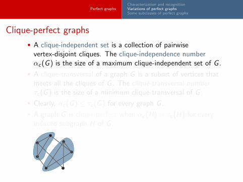
A clique-independent set is a collection of pairwisevertex-disjoint cliques. The clique-independence numberαc(G ) is the size of a maximum clique-independent set of G .
A clique-transversal of a graph G is a subset of vertices thatmeets all the cliques of G . The clique-transversal numberτc(G ) is the size of a minimum clique-transversal of G .
Clearly, αc(G ) ≤ τc(G ) for every graph G .
A graph G is clique-perfect when αc(H) = τc(H) for everyinduced subgraph H of G .

Perfect graphsCharacterization and recognitionVariations of perfect graphsSome subclasses of perfect graphs
Clique-perfect graphs
The terminology “clique-perfect” has been introduced byGuruswami and Pandu Rangan in 2000, but the equality ofthe parameters αc and τc was previously studied by Berge inthe seventies.
Guruswami Pandu Rangan
The complete list of minimal clique-imperfect graphs is stillnot known. Another open question concerning clique-perfectgraphs is the complexity of the recognition problem.

Perfect graphsCharacterization and recognitionVariations of perfect graphsSome subclasses of perfect graphs
Question: is there some relation between clique-perfectgraphs and perfect graphs?
Odd holes C2k+1, k ≥ 2, are not clique-perfect:αc(C2k+1) = k and τc(C2k+1) = k + 1.
Antiholes Cn, n ≥ 5, are clique-perfect if and only if n ≡ 0(3)(Reed, 2000): τc(Cn) = 3 and αc(Cn) = 2 or 3, being 3 onlyif n is divisible by three.
C5 C7 C9

Perfect graphsCharacterization and recognitionVariations of perfect graphsSome subclasses of perfect graphs
So we have the following scheme of relation between perfectgraphs and clique-perfect graphs:
C 6k±1
C 6k±2 C 6kC 6k+3
perfect clique-perfect

Perfect graphsCharacterization and recognitionVariations of perfect graphsSome subclasses of perfect graphs
In several works, clique-perfect graphs have been characterized bya restricted list of forbidden induced subgraphs when the graphbelongs to a certain class. Some of this characterizations lead topolynomial time recognition algorithms for clique-perfection withinthese classes.
J. Lehel and Z. Tuza, Neighborhood perfect graphs, DiscreteMathematics 61 (1986), 93–101.
F. Bonomo, M. Chudnovsky and G.D., Partialcharacterizations of clique-perfect graphs, Electronic Notes inDiscrete Mathematics 19 (2005), 95–101.
F. Bonomo and G.D., Characterization and recognition ofHelly circular-arc clique-perfect graphs, Electronic Notes inDiscrete Mathematics 22 (2005), 147–150.

Perfect graphsCharacterization and recognitionVariations of perfect graphsSome subclasses of perfect graphs
Example: The characterization for line graphsLet H be a graph. Its line graph L(H) is the intersection graph ofthe edges of H. A graph G is a line graph if there exists a graph Hsuch that G = L(H).
Theorem
Let G be a line graph. Then the following statements areequivalent:
1. No induced subgraph of G is and odd hole, or a pyramid.
2. G is clique-perfect.
3. G is perfect and it does not contain a pyramid.
pyramid

Perfect graphsCharacterization and recognitionVariations of perfect graphsSome subclasses of perfect graphs
Example: The characterization for line graphs
Line graphs have polynomial time recognition (Lehot, 1974).
The recognition of clique-perfect line graphs can be reduced to therecognition of perfect graphs with no pyramid, which is solvable inpolynomial time.
pyramid

Perfect graphsCharacterization and recognitionVariations of perfect graphsSome subclasses of perfect graphs
Coordinated graphs
Let v be a vertex of a graph G and m(v) the number ofcliques containing v .
Let M(G ) be the maximum m(v) for any v in G .
Let F (G ) be the cardinality of a minimum partition of thecliques of G into clique-independent sets, that is, the smallestnumber of colors that can be assigned to the cliques of G sothat intersecting cliques have different colors.
Note that F (G ) ≥ M(G ) for any graph G .
m(v) = 3,m(w) = 1,M = 3
F = 4

Perfect graphsCharacterization and recognitionVariations of perfect graphsSome subclasses of perfect graphs
Coordinated graphs
Let v be a vertex of a graph G and m(v) the number ofcliques containing v .
Let M(G ) be the maximum m(v) for any v in G .
Let F (G ) be the cardinality of a minimum partition of thecliques of G into clique-independent sets, that is, the smallestnumber of colors that can be assigned to the cliques of G sothat intersecting cliques have different colors.
Note that F (G ) ≥ M(G ) for any graph G .
m(v) = 3,m(w) = 1,M = 3 F = 4

Perfect graphsCharacterization and recognitionVariations of perfect graphsSome subclasses of perfect graphs
Coordinated graphs
We say that a graph G is coordinated if F (H) = M(H), forevery induced subgraph H of G (this class of graph wasdefined by Bonomo, D. and Groshaus in 2002).
Property: Coordinated graphs are perfect.
The complete list of minimal non-coordinated graphs is stillnot known. Again, they have been characterized by arestricted list of forbidden induced subgraphs when the graphbelongs to a certain class (Bonomo, D., Soulignac and Sueiro,2006).

Perfect graphsCharacterization and recognitionVariations of perfect graphsSome subclasses of perfect graphs
Example: The characterization for complements of forests
A forest is a graph with no cycles.
Theorem
Let G be a complement of a forest. Then G is coordinated if andonly if G contains neither 2P4 nor R as induced subgraphs.
2P4 and R
This theorem leads to a linear time recognition of coordinatedgraphs if the given graph is a complement of a forest.
The general recognition of coordinated graphs is NP-hard(Soulignac and Sueiro, 2006).

Perfect graphsCharacterization and recognitionVariations of perfect graphsSome subclasses of perfect graphs
Some subclasses of perfect graphs
A graph is an interval graph if it is the intersection graph of aset of intervals over the real line. A unit interval graph is theintersection graph of a set of intervals of length one.
A split graph is a graph whose vertex set can be partitionedinto a complete graph K and a stable set S . A split graph issaid to be complete if its edge set includes all possible edgesbetween K and S .
A bipartite graph is a graph whose vertex set can bepartitioned into two independent sets V1 and V2. A bipartitegraph is said to be complete if its edge set includes allpossible edges between V1 and V2.

Perfect graphsCharacterization and recognitionVariations of perfect graphsSome subclasses of perfect graphs
Some subclasses of perfect graphs
A cograph is a graph with no induced P4.
The line graph of a graph is the intersection graph of itsedges. Line graphs of bipartite graphs are perfect.
A graph is distance-hereditary if the distance between any twovertices in a connected induced subgraph containing both isthe same as in the original graph.
A graph is a block graph if it is connected and every maximal2-connected component is complete.

Extensions of the coloring problem
Problems descriptionGeneral resultsReview of computational complexitiesSome proofs
Extensions of the coloring problem

Extensions of the coloring problem
Problems descriptionGeneral resultsReview of computational complexitiesSome proofs
The list-coloring problemIn order to take into account particular constraints arising inpractical settings, more elaborate models of vertex coloring havebeen defined in the literature. One of such generalized models isthe list-coloring problem, which considers a prespecified set ofavailable colors for each vertex.
Given a graph G and a finite list L(v) ⊆ N for each vertexv ∈ V , the list-coloring problem asks for a list-coloring of G ,i.e., a coloring f such that f (v) ∈ L(v) for every v ∈ V .
1,2
1,3
1
2,3
3
2,3
21,3
1,2
1,3
1
2,3
3
2,3
21,3
3
3
3
2
2
2
1
1

Extensions of the coloring problem
Problems descriptionGeneral resultsReview of computational complexitiesSome proofs
The list-coloring problem
Many classes of graphs where the vertex coloring problem ispolynomially solvable are known, the most prominent beingthe class of perfect graphs [Grotschel-Lovasz-Schrijver, 1981].
Meanwhile, the list-coloring problem is NP-complete forperfect graphs, and is also NP-complete for many subclassesof perfect graphs, including split graphs, interval graphs, andbipartite graphs.
Trees and complete graphs are two classes of graphs wherethe list-coloring problem can be solved in polynomial time. Inthe first case it can be solved using dynamic programmingtechniques [Jansen-Scheffler, 1997]. In the second case, theproblem can be reduced to the maximum matching problem inbipartite graphs.

Extensions of the coloring problem
Problems descriptionGeneral resultsReview of computational complexitiesSome proofs
We are going to explore the complexity boundary between vertexcoloring and list-coloring in different subclasses of perfect graphs.The goal is to analyze the computational complexity of coloringproblems lying “between” (from a computational complexityviewpoint) these two problems.

Extensions of the coloring problem
Problems descriptionGeneral resultsReview of computational complexitiesSome proofs
The precoloring extension problemSome particular cases of list-coloring have been studied.
The precoloring extension (PrExt) problem takes as input agraph G = (V ,E ), a subset W ⊆ V , a coloring f ′ of W , anda natural number k, and consists in deciding whether Gadmits a k-coloring f such that f (v) = f ′(v) for every v ∈ Wor not [Biro-Hujter-Tuza, 1992].
In other words, a prespecified vertex subset is colored beforehand,and our task is to extend this partial coloring to a valid k-coloringof the whole graph.
k=3
1
2
k=3
1
1
2
2
2 2
33

Extensions of the coloring problem
Problems descriptionGeneral resultsReview of computational complexitiesSome proofs
The µ-coloring problem
Another particular case of the list-coloring problem is the following.
Given a graph G and a function µ : V → N, G is µ-colorableif there exists a coloring f of G such that f (v) ≤ µ(v) forevery v ∈ V [Bonomo-Cecowski, 2005].
This model arises in the context of classroom allocation to courses,where each course must be assigned a classroom which is largeenough so it fits the students taking the course.
1
2
3
2
<
<
<
<
<
<
<
<
3
3
3
2
1
2
3
2
3
3
3
2
2
2
1
1
<
<
<
<
<
<
<
<
3
3
3
2
Extensions of the coloring problem
Problems descriptionGeneral resultsReview of computational complexitiesSome proofs
The (γ, µ)-coloring problem
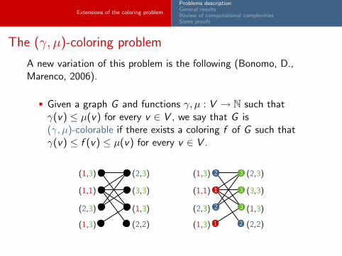
A new variation of this problem is the following (Bonomo, D.,Marenco, 2006).
Given a graph G and functions γ, µ : V → N such thatγ(v) ≤ µ(v) for every v ∈ V , we say that G is(γ, µ)-colorable if there exists a coloring f of G such thatγ(v) ≤ f (v) ≤ µ(v) for every v ∈ V .
(1,3)
(1,3)
(1,1)
(2,3)
(3,3)
(2,3)
(2,2)(1,3)
(1,3)
(1,3)
(1,1)
(2,3)
(3,3)
(2,3)
(2,2)(1,3) 1
1
2
2
2
3
3
3

Extensions of the coloring problem
Problems descriptionGeneral resultsReview of computational complexitiesSome proofs
The classical vertex coloring problem is clearly a special caseof µ-coloring and precoloring extension, which in turn arespecial cases of (γ, µ)-coloring.
Furthermore, (γ, µ)-coloring is a particular case oflist-coloring.
These observations imply that all the problems in thishierarchy are polynomially solvable in those graph classeswhere list-coloring is polynomial and, on the other hand, allthe problems are NP-complete in those graph classes wherevertex coloring is NP-complete.

Extensions of the coloring problem
Problems descriptionGeneral resultsReview of computational complexitiesSome proofs
General results
Since all the problems are NP-complete in the general case, thereare also polynomial-time reductions from list-coloring toprecoloring extension and µ-coloring. An example is shown in thefigure, where we can see a list-coloring instance and itscorresponding precoloring extension and µ-coloring instances.
3
4
2
1
3<
1<
2<< 4
2
1,42,3
1,32
3
1
4
4
k=4
3<3<
2<
1<
1<
1<2<
These reductions involve changes in the graph, but are closedwithin some graph classes. This fact allows us to prove thefollowing general results.

Extensions of the coloring problem
Problems descriptionGeneral resultsReview of computational complexitiesSome proofs
General results
Theorem
Let F be a family of graphs with minimum degree at least two. Thenlist-coloring, (γ, µ)-coloring and precoloring extension are polynomiallyequivalent in the class of F-free graphs.
Theorem
Let F be a family of graphs satisfying the following property: for everygraph G in F , no connected component of G is complete, and for everycutpoint v of G , no connected component of G \ v is complete. Thenlist-coloring, (γ, µ)-coloring, µ-coloring and precoloring extension arepolynomially equivalent in the class of F-free graphs.
Since odd holes and antiholes satisfy the conditions of the theoremsabove, these theorems are applicable for many subclasses of perfectgraphs.

Extensions of the coloring problem
Problems descriptionGeneral resultsReview of computational complexitiesSome proofs
Review: complexity table for coloring problems
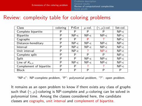
Class coloring PrExt µ-col. (γ, µ)-col. list-col.Complete bipartite P P P P NP-cBipartite P NP-c NP-c NP-c NP-cCographs P P P ? NP-cDistance-hereditary P NP-c NP-c NP-c NP-cInterval P NP-c NP-c NP-c NP-cUnit interval P NP-c ? NP-c NP-cComplete split P P P P NP-cSplit P P NP-c NP-c NP-cLine of Kn,n P NP-c NP-c NP-c NP-cComplement of bipartite P P ? ? NP-cBlock P P P P P
“NP-c”: NP-complete problem, “P”: polynomial problem, “?”: open problem.
As this table shows, unless P = NP, µ-coloring and precoloring extensionare strictly more difficult than vertex coloring, list-coloring is strictly moredifficult than (γ, µ)-coloring and (γ, µ)-coloring is strictly more difficultthan precoloring extension.

Extensions of the coloring problem
Problems descriptionGeneral resultsReview of computational complexitiesSome proofs
Review: complexity table for coloring problems
Class coloring PrExt µ-col. (γ, µ)-col. list-col.Complete bipartite P P P P NP-cBipartite P NP-c NP-c NP-c NP-cCographs P P P ? NP-cDistance-hereditary P NP-c NP-c NP-c NP-cInterval P NP-c NP-c NP-c NP-cUnit interval P NP-c ? NP-c NP-cComplete split P P P P NP-cSplit P P NP-c NP-c NP-cLine of Kn,n P NP-c NP-c NP-c NP-cComplement of bipartite P P ? ? NP-cBlock P P P P P
“NP-c”: NP-complete problem, “P”: polynomial problem, “?”: open problem.
As this table shows, unless P = NP, µ-coloring and precoloring extensionare strictly more difficult than vertex coloring, list-coloring is strictly moredifficult than (γ, µ)-coloring and (γ, µ)-coloring is strictly more difficultthan precoloring extension.
Extensions of the coloring problem
Problems descriptionGeneral resultsReview of computational complexitiesSome proofs
Review: complexity table for coloring problems
Class coloring PrExt µ-col. (γ, µ)-col. list-col.Complete bipartite P P P P NP-cBipartite P NP-c NP-c NP-c NP-cCographs P P P ? NP-cDistance-hereditary P NP-c NP-c NP-c NP-cInterval P NP-c NP-c NP-c NP-cUnit interval P NP-c ? NP-c NP-cComplete split P P P P NP-cSplit P P NP-c NP-c NP-cLine of Kn,n P NP-c NP-c NP-c NP-cComplement of bipartite P P ? ? NP-cBlock P P P P P
“NP-c”: NP-complete problem, “P”: polynomial problem, “?”: open problem.
It remains as an open problem to know if there exists any class of graphssuch that (γ, µ)-coloring is NP-complete and µ-coloring can be solved inpolynomial time. Among the classes considered here, the candidateclasses are cographs, unit interval and complement of bipartite.

Extensions of the coloring problem
Problems descriptionGeneral resultsReview of computational complexitiesSome proofs
Review: complexity table for coloring problems
Class coloring PrExt µ-col. (γ, µ)-col. list-col.Complete bipartite P P P P NP-cBipartite P NP-c NP-c NP-c NP-cCographs P P P ? NP-cDistance-hereditary P NP-c NP-c NP-c NP-cInterval P NP-c NP-c NP-c NP-cUnit interval P NP-c ? NP-c NP-cComplete split P P P P NP-cSplit P P NP-c NP-c NP-cLine of Kn,n P NP-c NP-c NP-c NP-cComplement of bipartite P P ? ? NP-cBlock P P P P P
“NP-c”: NP-complete problem, “P”: polynomial problem, “?”: open problem.
For split graphs, precoloring extension can be solved in polynomial time,whereas µ-coloring is NP-complete. It remains as an open problem tofind a class of graphs where the converse holds. Among the classesconsidered here, the candidate class is unit interval.

Extensions of the coloring problem
Problems descriptionGeneral resultsReview of computational complexitiesSome proofs
Review: hierarchy of coloring problems
list-coloring
k-coloring
(γ,µ)-coloring
PrExt µ-coloring
<<
<
< <

Extensions of the coloring problem
Problems descriptionGeneral resultsReview of computational complexitiesSome proofs
(γ, µ)-coloring is polynomial for complete bipartite graphs
Proof: The following is a combinatorial algorithm that solves(γ, µ)-coloring in polynomial time for complete bipartite graphs.
Let G = (V ,E ) be a complete bipartite graph, with bipartitionV1 ∪ V2, and let γ, µ : V → N such that γ(v) ≤ µ(v) for everyv ∈ V .
We have to consider two cases:
(i) There exists a vertex v such that γ(v) = µ(v).
(ii) For every vertex v , γ(v) < µ(v).
(1,3)
(1,3)
(1,1)
(2,3)
(3,3)
(2,3)
(2,2)(1,3)
21 3
Extensions of the coloring problem
Problems descriptionGeneral resultsReview of computational complexitiesSome proofs
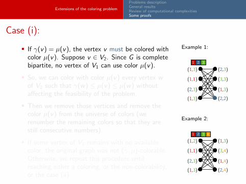
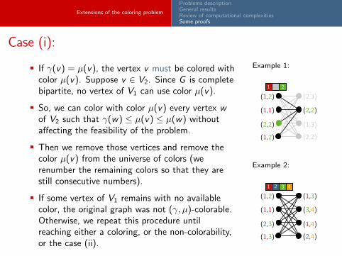
Case (i):
If γ(v) = µ(v), the vertex v must be colored withcolor µ(v). Suppose v ∈ V2. Since G is completebipartite, no vertex of V1 can use color µ(v).
So, we can color with color µ(v) every vertex wof V2 such that γ(w) ≤ µ(v) ≤ µ(w) withoutaffecting the feasibility of the problem.
Then we remove those vertices and remove thecolor µ(v) from the universe of colors (werenumber the remaining colors so that they arestill consecutive numbers).
If some vertex of V1 remains with no availablecolor, the original graph was not (γ, µ)-colorable.Otherwise, we repeat this procedure untilreaching either a coloring, or the non-colorability,or the case (ii).
Example 1:
(1,3)
(1,3)
(1,1)
(2,3)
(3,3)
(2,3)
(2,2)(1,3)
21 3
Example 2:
(1,2)
(1,4)
(1,1)
(1,3)
(3,4)
(2,3)
(2,4)(1,3)
21 3 4

Extensions of the coloring problem
Problems descriptionGeneral resultsReview of computational complexitiesSome proofs
Case (i):
If γ(v) = µ(v), the vertex v must be colored withcolor µ(v). Suppose v ∈ V2. Since G is completebipartite, no vertex of V1 can use color µ(v).
So, we can color with color µ(v) every vertex wof V2 such that γ(w) ≤ µ(v) ≤ µ(w) withoutaffecting the feasibility of the problem.
Then we remove those vertices and remove thecolor µ(v) from the universe of colors (werenumber the remaining colors so that they arestill consecutive numbers).
If some vertex of V1 remains with no availablecolor, the original graph was not (γ, µ)-colorable.Otherwise, we repeat this procedure untilreaching either a coloring, or the non-colorability,or the case (ii).
Example 1:
(1,2)
(1,3)
(1,1)
(2,3)
(2,2)
(2,2)
(2,2)(1,2)
1 2
Example 2:
(1,2)
(1,4)
(1,1)
(1,3)
(3,4)
(2,3)
(2,4)(1,3)
21 3 4

Extensions of the coloring problem
Problems descriptionGeneral resultsReview of computational complexitiesSome proofs
Case (i):
If γ(v) = µ(v), the vertex v must be colored withcolor µ(v). Suppose v ∈ V2. Since G is completebipartite, no vertex of V1 can use color µ(v).
So, we can color with color µ(v) every vertex wof V2 such that γ(w) ≤ µ(v) ≤ µ(w) withoutaffecting the feasibility of the problem.
Then we remove those vertices and remove thecolor µ(v) from the universe of colors (werenumber the remaining colors so that they arestill consecutive numbers).
If some vertex of V1 remains with no availablecolor, the original graph was not (γ, µ)-colorable.Otherwise, we repeat this procedure untilreaching either a coloring, or the non-colorability,or the case (ii).
Example 1:
(1,2)
(1,3)
(1,1)
(2,3)
()
(2,2)
(2,2)(1,2)
1
Example 2:
(1,2)
(2,4)
(1,1)
(2,3)
(3,4)
(2,3)
(2,4)(1,3)
2 3 4

Extensions of the coloring problem
Problems descriptionGeneral resultsReview of computational complexitiesSome proofs
Case (ii):
If for every vertex v , γ(v) < µ(v), then every vertex hasamong its possible colors at least an odd color and an evencolor.
So the graph is (γ, µ)-colorable, we can color the vertices ofV1 with odd colors and the vertices of V2 with even colors.
(1,2)
(2,4)
(1,1)
(2,3)
(3,4)
(2,3)
(2,4)(1,3)
2 3 4
2

Extensions of the coloring problem
Problems descriptionGeneral resultsReview of computational complexitiesSome proofs
Case (ii):
If for every vertex v , γ(v) < µ(v), then every vertex hasamong its possible colors at least an odd color and an evencolor.
So the graph is (γ, µ)-colorable, we can color the vertices ofV1 with odd colors and the vertices of V2 with even colors.
(1,2)
(1,4)
(1,1)
(1,3)
(3,4)
(2,3)
(2,4)(1,3)
21 3 4
2

Extensions of the coloring problem
Problems descriptionGeneral resultsReview of computational complexitiesSome proofs
µ-coloring is NP-complete for split graphsProof: It is used a reduction from the dominating set problem onsplit graphs, which is NP-complete (A. Bertossi, 1984).
An instance of the dominating set problem on split graphs is givenby a split graph G and an integer k ≥ 1, and consists in deciding ifthere exists a subset D of V (G ), with |D| ≤ k, and such thatevery vertex of V (G ) either belongs to D or has a neighbor in D.Such a set is called a dominating set.
k=3
dominating set

Extensions of the coloring problem
Problems descriptionGeneral resultsReview of computational complexitiesSome proofs
Let G be a split graph and k ≥ 0; V (G ) = K ∪ I , K is a completeand I is an independent set. We may assume G with no isolatedvertices and k ≤ |K |.
We will construct a split graph G ′ and a functionµ : V (G ′) → N such that G ′ is µ-colorable if and only if Gadmits a dominating set of cardinality at most k:
V (G ′) = K ∪ IK is a complete and I is an independent set in G ′
for v ∈ K and w ∈ I , vw ∈ E (G ′) iff vw 6∈ E (G )µ(v) = |K | for v ∈ K and µ(w) = k for w ∈ I .
instance of split dominating set instance of split µ-coloring

Extensions of the coloring problem
Problems descriptionGeneral resultsReview of computational complexitiesSome proofs
Suppose first that G admits a dominating set D with |D| ≤ k.Since G has no isolated vertices, G admits such a set D ⊆ K .
dominating set
µ-coloring
Let us define a µ-coloring of G ′ as follows:
color the vertices of D using different colors from 1 to |D|color the remaining vertices of K using different colors from|D|+ 1 to |K |for each vertex w in I , choose w ′ in D such that ww ′ ∈ E (G )and color w with the color used by w ′.

Extensions of the coloring problem
Problems descriptionGeneral resultsReview of computational complexitiesSome proofs
Suppose first that G admits a dominating set D with |D| ≤ k.Since G has no isolated vertices, G admits such a set D ⊆ K .
dominating set µ-coloring
Let us define a µ-coloring of G ′ as follows:
color the vertices of D using different colors from 1 to |D|color the remaining vertices of K using different colors from|D|+ 1 to |K |for each vertex w in I , choose w ′ in D such that ww ′ ∈ E (G )and color w with the color used by w ′.

Extensions of the coloring problem
Problems descriptionGeneral resultsReview of computational complexitiesSome proofs
Suppose now that G ′ is µ-colorable, and let c : V (G ′) → Nbe a µ-coloring of G ′. Since µ(v) = |K | for every v ∈ K andK is complete in G ′, it follows that c(K ) = {1, . . . , |K |}.
µ-coloring
dominating set
Since k ≤ |K |, for each vertex w ∈ I there is a vertex w ′ ∈ Ksuch that c(w) = c(w ′) ≤ k. Then ww ′ 6∈ E (G ′), soww ′ ∈ E (G ). Thus the set {v ∈ K : c(v) ≤ k} is adominating set of G of size k.
2

Extensions of the coloring problem
Problems descriptionGeneral resultsReview of computational complexitiesSome proofs
Suppose now that G ′ is µ-colorable, and let c : V (G ′) → Nbe a µ-coloring of G ′. Since µ(v) = |K | for every v ∈ K andK is complete in G ′, it follows that c(K ) = {1, . . . , |K |}.
µ-coloring dominating set
Since k ≤ |K |, for each vertex w ∈ I there is a vertex w ′ ∈ Ksuch that c(w) = c(w ′) ≤ k. Then ww ′ 6∈ E (G ′), soww ′ ∈ E (G ). Thus the set {v ∈ K : c(v) ≤ k} is adominating set of G of size k.
2

Extensions of the coloring problem
Problems descriptionGeneral resultsReview of computational complexitiesSome proofs
Acknowledgments: To Flavia Bonomo for her valuable help in thepreparation of this course.