graph theory and incentives - jesus & mary college · graph theory and incentives ... i problem...
TRANSCRIPT

Graph Theory and Incentives
Debasis MishraIndian Statistical Institute (ISI)
August 11, 2017

Outline of the talk
I Problem 1: Incentivizing truth-telling
I Graph theory and Farkas Lemma
I Problem 2: Reduced form auctions (time permitting)

Incentivizing truth-telling by payments
If payments are not allowed, it is difficult to incentivize individualsto tell the truth.
Example: In voting environment, the only truthful and unanimousvoting rule is a dictatorship.
Payments expand the possibility of incentivizing truth-telling.

Incentivizing truth-telling by payments
If payments are not allowed, it is difficult to incentivize individualsto tell the truth.
Example: In voting environment, the only truthful and unanimousvoting rule is a dictatorship.
Payments expand the possibility of incentivizing truth-telling.

Uses of payments
Many strategic interactions allow for the possibility of payments.
I Bilateral trading: a buyer and a seller meet and trade anobject that the seller owns by using payments.
I Auctions: bidders bid on objects and pay for them.
I Public good provision: deciding to build a nuclear plant in aneighborhood, some citizens may be taxed for it and somepeople may be subsidized.

Mechanism design with payments
Designing games where payments are allowed to induce “desired”equilibrium behavior.
One of the most successful branches of game theory in terms ofreal-life applications: auctions of all kinds.

Spectrum auctions
Govt owns many natural resources - some of them were exclusiveto Govt (for instance spectrum waves, coal mines).
These resources found their use beyond Govt - for instance,spectrum waves became useful outside defense with the arrival ofdigital communication.
They were sold using auctions - a country is divided into blocks or“circles” and the entire set of blocks are sold simulatenously usingauction (where bidders can claim any subset of objects).
Huge success of some spectrum auctions all over the world: interms of revenues achieved.

Internet advertisingMajor source of revenue for Google, Microsoft come from their saleof “display and search advertising slots”.
About 7,37,00,000 results (0.52 seconds)
Report images
Cute WalkSports Shoes...₹ 484.25FirstCry India
Lotto LegendWhite & Navy...₹ 1,319.00TataCLiQ.com
Nivia YorksRunning ...₹ 929.00Schoolkart
Lotto HurryBlack & Blue ...₹ 1,379.00TataCLiQ.com
ProvogueRunningShoes₹ 499.00Flipkart
Earton Men'sWhite EVA ...₹ 298.00Amazon India
Images for Running Shoes
More images for Running Shoes
SponsoredShop for Running Shoes on Google
Running Shoes - 40% to 70% Off On Select Brands - amazon.in Ad www.amazon.in/Running+Shoes Easy Returns & Pay On Delivery!100% Purchase Protection · Cash on Delivery · Huge Selection · Free Shipping*Types: Casual Shoes, Formal Shoes, Sports Shoes, Sandals & Floaters, Flip-flops, Boots, Sneakers, …Mens Shoes · Sales & Deals · Womens Shoes · Kids Shoes
Buy Running Shoes Online - Get Up to 60% Off On Shoes - abof.comAd www.abof.com/Shoes/RunningUse Coupon ABOFSS100 For Rs 100 Off On a Purchase of Rs 1295. Hurry!Hassle Free Returns · Curated Merchandise · Spring-Summer Collections · Cash On Delivery
Running Shoes for Men - Buy Shoes Online in India | Jabong.comwww.jabong.com › Men › ShoesBuy Men's Running Shoes Online in India. Select from the best range of Running Shoes atJabong.com. ✓ easy shipping ✓ 15 days Return ✓ Cash on Delivery ...
Running Shoes - Buy Running Shoes Online at Best Prices in India ...www.flipkart.com › Footwear › Men's Footwear › Sports ShoesShop Running Shoes Online and Check Latest Running Shoes Collections with Price and excitingoffers in India's favourite Online Shopping Site.
Amazon.in: Running Shoes: Shoes & Handbagswww.amazon.in/Mens-Running-Shoes/b?ie=UTF8&node=1983550031Results 1 - 60 of 7427 - Online shopping for Running Shoes from a great selection at Shoes &Handbags Store.
Mens Running Shoes at SportsDirect.comwww.sportsdirect.com › Running › Running ShoesImprove your personal best with our fantastic collection of men's running shoes and trainers fromspecialist running brands such as Nike, adidas, Karrimor and ...
Men's Running Shoes at Road Runner Sportswww.roadrunnersports.com/rrs/mensshoes/mensshoesrunning/Get the best running shoes for men at Road Runner Sports based on your arch type, body type &running terrain. Shop now!
Running Shoes | Zappos.com FREE Shipping | Zappos.comwww.zappos.com/running-shoesRunning Shoes Neutral Running Shoes Crosstraining Shoes Stability Running Shoes Trail RunningShoes Running Clothing & Activewear Running Tops, Tees, ...
Sneakers & Athletic Shoes, Running | Shipped Free at Zapposwww.zappos.com/sneakers-athletic-shoes/CK_XARC81wE6Ap4L.zso2536 items - Free shipping BOTH ways on Sneakers & Athletic Shoes, Running, from our vast
All Images News Videos Search toolsMore
A simple model
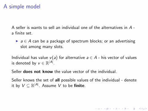
A seller is wants to sell an individual one of the alternatives in A -a finite set.
I a ∈ A can be a package of spectrum blocks; or an advertisingslot among many slots.
Individual has value v(a) for alternative a ∈ A - his vector of valuesis denoted by v ∈ R|A|.
Seller does not know the value vector of the individual.
Seller knows the set of all possible values of the individual - denoteit by V ⊆ R|A|. Assume V to be finite.

Rules
Allocation rule is a map
f : V → A.
It specifies what the seller would like to sell to the individual if heknew the values.
Payments are possible (and used to induce incentives). A paymentrule is a map
p : V → R.
Utility of individual: if the individual with value vector v getsalternative a ∈ A and pays an amount p, then his net payoff is
v(a)− p,
where p can be positive, negative, or zero also.

Mechanism
Mechanism (f , p):
I Seller asks the individual to announce a value vector in V .
I The individual announces a value vector in V (may not be histrue value vector).
I If v ′ ∈ V is announced, individual gets f (v ′) ∈ A and paysp(v ′).
I His utility isv(f (v ′))− p(v ′).

Implementing truth
DefinitionAn allocation rule f can be truthfully implemented if there existsp : V → R such that
v(f (v))− p(v) ≥ v(f (v ′))− p(v ′) ∀ v , v ′ ∈ V .
Which f can be truthfully implemented?
Not every f can be . . .
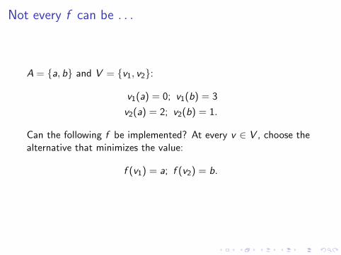
A = {a, b} and V = {v1, v2}:
v1(a) = 0; v1(b) = 3
v2(a) = 2; v2(b) = 1.
Can the following f be implemented? At every v ∈ V , choose thealternative that minimizes the value:
f (v1) = a; f (v2) = b.

Not every f can be . . .
Suppose f can be truthfully implemented. Then there exists p(v1)and p(v2) such that
0− p(v1) = v1(f (v1))− p(v1) ≥ v1(f (v2))− p(v2) = 3− p(v2)
1− p(v2) = v2(f (v2))− p(v2) ≥ v2(f (v1))− p(v1) = 2− p(v1).
Adding these gives us 1 ≥ 5 - a contradiction.

Towards a necessary condition
Suppose f can be truthfully implemented. Then, there existsp : V → R that implements it.
Consider a cycle of incentive constraints:
v1 → v2 → . . .→ vm → v1.

Incentive constraints along a cycle
v1(f (v1))− p(v1) ≥ v1(f (v2))− p(v2)
v2(f (v2))− p(v2) ≥ v2(f (v3))− p(v3)
. . . ≥ . . .
. . . ≥ . . .vm(f (vm))− p(vm) ≥ vm(f (v1))− p(v1).
The p terms cancel out in telescopic sum.

Incentive constraints along a cycle
v1(f (v1))− p(v1) ≥ v1(f (v2))− p(v2)
v2(f (v2))− p(v2) ≥ v2(f (v3))− p(v3)
. . . ≥ . . .
. . . ≥ . . .vm(f (vm))− p(vm) ≥ vm(f (v1))− p(v1).
The p terms cancel out in telescopic sum.

Reinterpreting
Denote for every v , v ′ ∈ V ,
`f (v ′, v) = [v(f (v))− v(f (v ′))].
The necessary condition is
m∑r=1
`f (v r , v r+1) ≥ 0
DefinitionAn allocation rule f is cyclically monotone if for every sequenceof distinct value vectors (v1, v2, . . . , vr )
`f (v1, v2) + . . .+ `f (vr−1, vr ) + `f (vr , v1) ≥ 0.
Graph Interpretation
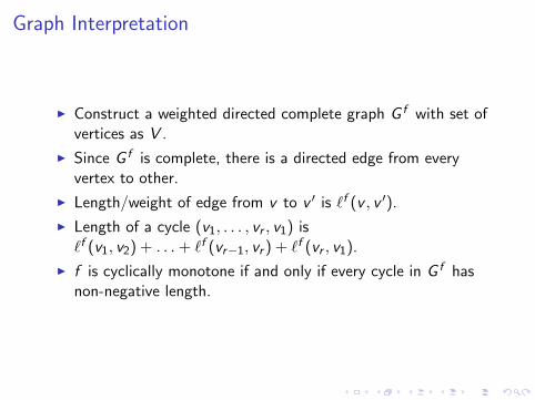
I Construct a weighted directed complete graph G f with set ofvertices as V .
I Since G f is complete, there is a directed edge from everyvertex to other.
I Length/weight of edge from v to v ′ is `f (v , v ′).
I Length of a cycle (v1, . . . , vr , v1) is`f (v1, v2) + . . .+ `f (vr−1, vr ) + `f (vr , v1).
I f is cyclically monotone if and only if every cycle in G f hasnon-negative length.

Illustration
v_3
−2
2
3
−1
0
1
v_1
v_2
Figure: Illustration of cycle monotonicity

Cycle monotonicity and implementation
TheoremAn allocation rule can be truthfully implemented if and only if it iscyclically monotone.

Two proofs
Proof 1. Direct - borrows results on “potential” functions in graphtheory.
Proof 2. Indirect - uses Farkas Lemma by considering the dual ofincentive constraints.

Directed graphs
A directed graph is defined by a set of vertices V and a set ofordered pairs (called edges) E := {(v , v ′) : v , v ′ ∈ V , v 6= v ′}.
A weighted directed graph is a directed graph with a weightfunction ` : E → R.
A potential function of a weighted directed graphG = ((V ,E ), `) is a map p : V → R such that
p(v)− p(v ′) ≤ `(v ′, v). ∀ (v ′, v) ∈ E

Cycles of directed graphs
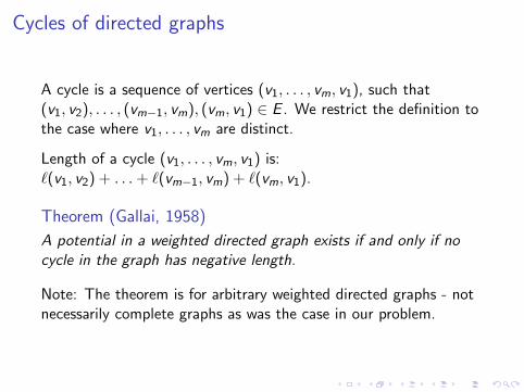
A cycle is a sequence of vertices (v1, . . . , vm, v1), such that(v1, v2), . . . , (vm−1, vm), (vm, v1) ∈ E . We restrict the definition tothe case where v1, . . . , vm are distinct.
Length of a cycle (v1, . . . , vm, v1) is:`(v1, v2) + . . .+ `(vm−1, vm) + `(vm, v1).
Theorem (Gallai, 1958)
A potential in a weighted directed graph exists if and only if nocycle in the graph has negative length.
Note: The theorem is for arbitrary weighted directed graphs - notnecessarily complete graphs as was the case in our problem.
Cycles of directed graphs
A cycle is a sequence of vertices (v1, . . . , vm, v1), such that(v1, v2), . . . , (vm−1, vm), (vm, v1) ∈ E . We restrict the definition tothe case where v1, . . . , vm are distinct.
Length of a cycle (v1, . . . , vm, v1) is:`(v1, v2) + . . .+ `(vm−1, vm) + `(vm, v1).
Theorem (Gallai, 1958)
A potential in a weighted directed graph exists if and only if nocycle in the graph has negative length.
Note: The theorem is for arbitrary weighted directed graphs - notnecessarily complete graphs as was the case in our problem.

Proof
Suppose a weighted directed graph G = ((V ,E ), `) has no cyclesof negative length.
If there is a vertex v0 ∈ V such that there is a path from v0 toevery other vertex, we choose that.
Else, construct a new graph G ′, where we put a dummy vertex v0and put edges (v0, vj) for all vj ∈ V .
The weights of new edges are zero: `(v0, vj) = 0 for all vj . So, wehave a new graph:
G ′ = ((V ∪ {v0},E ∪ {(v0, vj) : vj ∈ V }), `).

Illustration
Observation: If G has no cycles of negative length, G ′ also has nocycles of negative length.
1
2 3
45 −2
21
−3
4
1
4
2 −3 3
2
4−2
100
0 0
0
0
Note: G ′ = G if v0 can be chosen in V such that there is a pathfrom v0 to every other vertex.
Paths and shortest paths
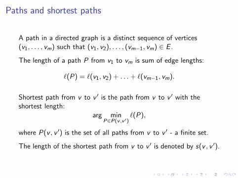
A path in a directed graph is a distinct sequence of vertices(v1, . . . , vm) such that (v1, v2), . . . , (vm−1, vm) ∈ E .
The length of a path P from v1 to vm is sum of edge lengths:
`(P) = `(v1, v2) + . . .+ `(vm−1, vm).
Shortest path from v to v ′ is the path from v to v ′ with theshortest length:
arg minP∈P(v ,v ′)
`(P),
where P(v , v ′) is the set of all paths from v to v ′ - a finite set.
The length of the shortest path from v to v ′ is denoted by s(v , v ′).

Illustration
v_3
−2
2
3
−1
0
1
v_1
v_2
Figure: Illustration of shortest paths
s(v2, v3) = −2.

Defining potentials
Define the following function:
p(v) = s(v0, v) ∀ v ∈ V .
Fix any v , v̂ ∈ V with (v , v̂) ∈ E . Two cases and show thatpotential inequalities hold.

Case 1
The shortest path from v0 to v does not include v̂ .
v0 v v̂
Then, shortest path from v0 to v and the direct edge (v , v̂) definesa path from v0 to v̂ .
s(v0, v̂) ≤ s(v0, v) + `(v , v̂). Hence,
p(v̂) ≤ p(v) + `(v , v̂).
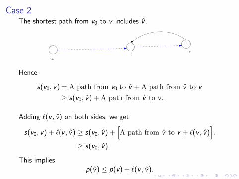
Case 2The shortest path from v0 to v includes v̂ .
v0
v̂v
Hence
s(v0, v) = A path from v0 to v̂ + A path from v̂ to v
≥ s(v0, v̂) + A path from v̂ to v .
Adding `(v , v̂) on both sides, we get
s(v0, v) + `(v , v̂) ≥ s(v0, v̂) +[A path from v̂ to v + `(v , v̂)
].
≥ s(v0, v̂).
This impliesp(v̂) ≤ p(v) + `(v , v̂).

Another construction
Instead of putting edges from dummy vertex to other vertices, putthem from other vertices to the dummy vertex (with zero length).
Define p(v) = −s(v , v0). for all v ∈ V . The same proof works andshows that this is a potential if no cycle has negative length.

Back to incentive problem
We are given f : V → A. We construct a complete directed graphwith edge lengths
`f (v ′, v) = v(f (v))− v(f (v ′)) ∀ v , v ′ ∈ V .
Denote this graph as G f - cycle monotonicity is no cycles ofnegative length in G f .
A potential function p : V → R of G f is a payment function thatsatisfies the incentive constraints:
p(v)− p(v ′) ≤ `f (v ′, v) = v(f (v))− v(f (v ′)) ∀ v , v ′ ∈ V .
So, f is truthfully implementable if and only if G f has no cycles ofnegative length.
Payments from G f
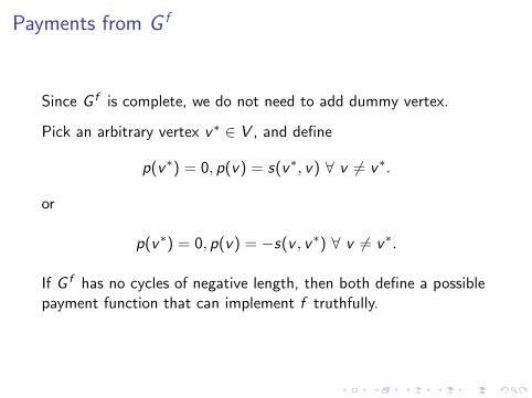
Since G f is complete, we do not need to add dummy vertex.
Pick an arbitrary vertex v∗ ∈ V , and define
p(v∗) = 0, p(v) = s(v∗, v) ∀ v 6= v∗.
or
p(v∗) = 0, p(v) = −s(v , v∗) ∀ v 6= v∗.
If G f has no cycles of negative length, then both define a possiblepayment function that can implement f truthfully.

A quick application
The seller has a cost vector κ : A→ R+ and for every v ,
f ∗(v) ∈ arg maxa∈A
[v(a)− κ(a)
].
Theoremf ∗ is truthfully implementable.

A quick application
Consider a cycle (v1, . . . , vm, v1) with f ∗ values (a1, . . . , am).Then, length of this cycle is[v1(a1)− v1(a2)
]+[v2(a2)− v2(a3)
]+ . . .+
[vm(am)− vm(a1)
]=[(v1(a1)− κ(a1))− (v1(a2)− κ(a2))
]+[(v2(a2)− κ(a2))− (v2(a3)− κ(a3))
]+ . . .
+[(vm(am)− κ(am))− (vm(a1)− κ(a1))
]≥ 0.

Infinite V sets
We assumed that V is finite. Not needed.
Suppose A is finite (as before) but V need not be finite.
Lemmaif f is implementable by p for any v , v ′ with f (v) = f (v ′) we havep(v) = p(v ′).
Suppose f (v) = f (v ′) = a, then incentive constraints v → v ′ andv ′ → v gives
v(a)− p(v) ≥ v(a)− p(v ′)
v ′(a)− p(v ′) ≥ v ′(a)− p(v).
This means p can be rewritten as a map p : A→ R.
Redefining incentive problem
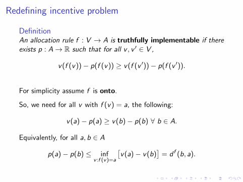
DefinitionAn allocation rule f : V → A is truthfully implementable if thereexists p : A→ R such that for all v , v ′ ∈ V ,
v(f (v))− p(f (v)) ≥ v(f (v ′))− p(f (v ′)).
For simplicity assume f is onto.
So, we need for all v with f (v) = a, the following:
v(a)− p(a) ≥ v(b)− p(b) ∀ b ∈ A.
Equivalently, for all a, b ∈ A
p(a)− p(b) ≤ infv :f (v)=a
[v(a)− v(b)
]= d f (b, a).

Redefining in a finite graph
DefinitionAn allocation rule f : V → A is truthfully implementable if thereexists p : A→ R such that for all a, b ∈ A,
p(a)− p(b) ≤ d f (b, a).
New graph H f : set of vertices A (a finite set), complete directedgraph, weight of edge (a, b) is d f (a, b).
f is truthfully implementable if and only if H f has no cycles ofnegative length.

More structure and deeper theorems
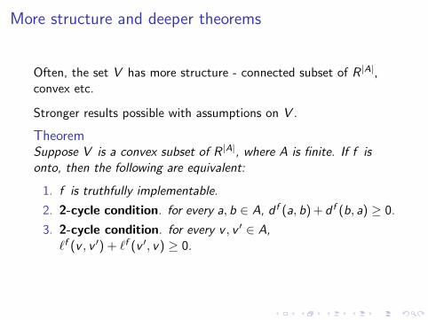
Often, the set V has more structure - connected subset of R |A|,convex etc.
Stronger results possible with assumptions on V .
TheoremSuppose V is a convex subset of R |A|, where A is finite. If f isonto, then the following are equivalent:
1. f is truthfully implementable.
2. 2-cycle condition. for every a, b ∈ A, d f (a, b) + d f (b, a) ≥ 0.
3. 2-cycle condition. for every v , v ′ ∈ A,`f (v , v ′) + `f (v ′, v) ≥ 0.
More structure and deeper theorems
Often, the set V has more structure - connected subset of R |A|,convex etc.
Stronger results possible with assumptions on V .
TheoremSuppose V is a convex subset of R |A|, where A is finite. If f isonto, then the following are equivalent:
1. f is truthfully implementable.
2. 2-cycle condition. for every a, b ∈ A, d f (a, b) + d f (b, a) ≥ 0.
3. 2-cycle condition. for every v , v ′ ∈ A,`f (v , v ′) + `f (v ′, v) ≥ 0.

A property of potentials
A potential function of a weighted directed graphG = ((V ,E ), `) is a map p : V → R such that
p(v)− p(v ′) ≤ `(v ′, v).
If p is a potential, then for any α ∈ R,
q(v) := p(v) + α ∀ v ∈ V
is also a potential function.
DefinitionA weighted directed graph satisfies potential equivalence if forany pair of potentials p, q, the following holds:
p(v)− q(v) = p(v ′)− q(v ′) ∀ v , v ′ ∈ V .

Why potential equivalence?
Finding one potential describes the entire set of potentials.
In our incentive problems, if we can find one payment function pthat implements f truthfully, we can describe the entire set ofpayment functions that implement f truthfully.
When does payoff equivalence hold?
We give an answer when G is a strongly connected graph - whichis the case for the graph induced by the incentive constraints.
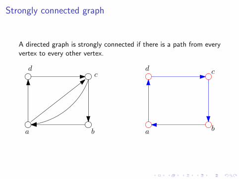
Strongly connected graph
A directed graph is strongly connected if there is a path from everyvertex to every other vertex.
a b
cd
a b
cd
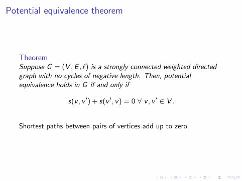
Potential equivalence theorem
TheoremSuppose G = (V ,E , `) is a strongly connected weighted directedgraph with no cycles of negative length. Then, potentialequivalence holds in G if and only if
s(v , v ′) + s(v ′, v) = 0 ∀ v , v ′ ∈ V .
Shortest paths between pairs of vertices add up to zero.

Proof of potential equivalence
Suppose potential equivalence holds. Fix v , v ′ ∈ V . Consider twopotentials
p(v) = 0, p(v̂) = s(v , v̂) ∀ v̂ 6= v .
q(v ′) = 0, p(v̂) = s(v ′, v̂) ∀ v̂ 6= v ′.
From our earlier proof, we know that both p and q are potentials.
Strong connectedness ensures that shortest paths exist.
By potential equivalence
−s(v ′, v) = p(v)− q(v) = p(v ′)− q(v ′) = s(v , v ′).

Proof of potential equivalence
Suppose for all v , v ′ we have s(v , v ′) + s(v ′, v) = 0.
Fix v , v ′ ∈ V and let (v = v0, v1, . . . , vk = v ′) be the shortest pathfrom v to v ′.
Pick a potential p (it exists since graph has no negative cycles)and add the potential constraints along the shortest path:
p(v1)− p(v0) ≤ `(v0, v1)
p(v2)− p(v1) ≤ `(v1, v2)
. . . ≤ . . .p(vk)− p(vk−1) ≤ `(vk−1, vk).

Proof of potential equivalence
Adding, we getp(v ′)− p(v) ≤ s(v , v ′).
Similarly, we get
p(v)− p(v ′) ≤ s(v ′, v) = −s(v , v ′).
This implies that
s(v , v ′) ≤ p(v ′)− p(v) ≤ s(v , v ′).
This gives us p(v ′)− p(v) = s(v , v ′) - since the RHS isindependent of the potential p, we get for any pair of potentialsp, q,
p(v ′)− p(v) = q(v ′)− q(v) = s(v , v ′).

Translating in incentive language
DefinitionAn implementable allocation rule f satisfies revenue equivalenceif for any pair of payment functions p, q implementing f , we have
p(v)− q(v) = p(v ′)− q(v ′) ∀ v , v ′ ∈ V .
The graph induced from an implementable f , H f , is always acomplete graph with no cycles of negative length (cyclemonotonicity).
Revenue equivalence of an implementable f holds if and only if inthe graph H f , we have s f (a, b) + s f (b, a) = 0 for all a, b ∈ A.

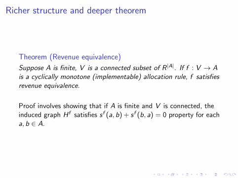
Richer structure and deeper theorem
Theorem (Revenue equivalence)
Suppose A is finite, V is a connected subset of R |A|. If f : V → Ais a cyclically monotone (implementable) allocation rule, f satisfiesrevenue equivalence.
Proof involves showing that if A is finite and V is connected, theinduced graph H f satisfies s f (a, b) + s f (b, a) = 0 property for eacha, b ∈ A.

The non-constructive proof
We now show a non-constructive proof of cycle monotonicityresult.
The proof works for finite V and uses the fact that the incentiveconstraints define a linear system of inequalities.
It then looks at the dual of this problem and then the theoremfollows immediately.

System of equations
x1 + x2 − 2x3 = 5
2x1 − x2 + 3x3 = 2
4x1 − x2 + 2x3 = 4
x1, x2, x3 ≥ 0
When do systems of linear equations/inequalties have non-negativesolutions?
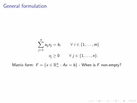
General formulation
n∑j=1
aijxj = bi ∀ i ∈ {1, . . . ,m}
xj ≥ 0 ∀ j ∈ {1, . . . , n}.
Matrix form: F = {x ∈ Rn+ : Ax = b} - When is F non-empty?
General idea of Farkas lemma
Farkas lemma provides an alternate system of inequalitieswhose infeasibility gives a certificate for the original system to benon-empty.
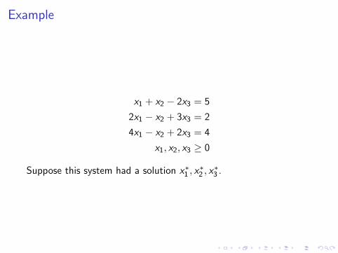
Example
x1 + x2 − 2x3 = 5
2x1 − x2 + 3x3 = 2
4x1 − x2 + 2x3 = 4
x1, x2, x3 ≥ 0
Suppose this system had a solution x∗1 , x∗2 , x∗3 .

Multipliers
Take multipliers y1, y2, y3 (one for each equation):
y1(x∗1 + x∗2 − 2x∗3 ) = 5y1
y2(2x∗1 − x∗2 + 3x∗3 ) = 2y2
y3(4x∗1 − x∗2 + 2x∗3 ) = 4y3
Adding them up gives
x∗1 (y1 + 2y2 + 4y3) + x∗2 (y1 − y2 − y3) + x∗3 (−2y1 + 3y2 + 2y3)
= (5y1 + 2y2 + 4y3).

Farkas alternative
y1 + 2y2 + 4y3 ≥ 0
y2 − y2 − y3 ≥ 0
−2y1 + 3y2 + 2y3 ≥ 0
5y1 + 2y2 + 4y3 < 0
has no solution.
The other direction is also true: If Farkas alternative has nosolution then original system has a solution.

Farkas alternative
y1 + 2y2 + 4y3 ≥ 0
y2 − y2 − y3 ≥ 0
−2y1 + 3y2 + 2y3 ≥ 0
5y1 + 2y2 + 4y3 < 0
has no solution.
The other direction is also true: If Farkas alternative has nosolution then original system has a solution.

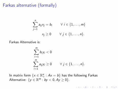
Farkas alternative (formally)
n∑j=1
aijxj = bi ∀ i ∈ {1, . . . ,m}
xj ≥ 0 ∀ j ∈ {1, . . . , n}.
Farkas Alternative is:
m∑i=1
biyi < 0
m∑i=1
aijyi ≥ 0 ∀ j ∈ {1, . . . , n}.
In matrix form {x ∈ Rn+ : Ax = b} has the following Farkas
Alternative: {y ∈ Rm : by < 0,Ay ≥ 0}.
Farkas alternative (formally)
n∑j=1
aijxj = bi ∀ i ∈ {1, . . . ,m}
xj ≥ 0 ∀ j ∈ {1, . . . , n}.
Farkas Alternative is:
m∑i=1
biyi < 0
m∑i=1
aijyi ≥ 0 ∀ j ∈ {1, . . . , n}.
In matrix form {x ∈ Rn+ : Ax = b} has the following Farkas
Alternative: {y ∈ Rm : by < 0,Ay ≥ 0}.
Farkas lemma
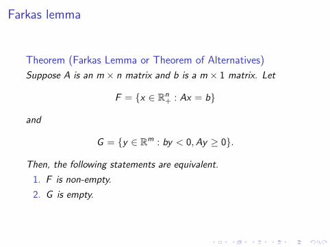
Theorem (Farkas Lemma or Theorem of Alternatives)
Suppose A is an m × n matrix and b is a m × 1 matrix. Let
F = {x ∈ Rn+ : Ax = b}
and
G = {y ∈ Rm : by < 0,Ay ≥ 0}.
Then, the following statements are equivalent.
1. F is non-empty.
2. G is empty.

One direction
Suppose (x∗1 , . . . , x∗n ) ∈ F . Then choose (y1, . . . , ym) such that
m∑i=1
aijyi ≥ 0 ∀ j ∈ {1, . . . , n}.
Since for every i ∈ {1, . . . ,m},
n∑j=1
aijx∗j = bi
⇒ yi
n∑j=1
aijx∗j = yibi .
One direction
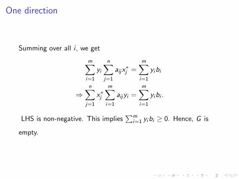
Summing over all i , we get
m∑i=1
yi
n∑j=1
aijx∗j =
m∑i=1
yibi
⇒n∑
j=1
x∗j
m∑i=1
aijyi =m∑i=1
yibi .
LHS is non-negative. This implies∑m
i=1 yibi ≥ 0. Hence, G is
empty.

Cones
Suppose A is an m × n matrix and let (a1, . . . , an) be the columnsof A. The set of all non-negative linear combinations of columns ofA is called the cone of A.
cone(A) = {b ∈ Rm :n∑
j=1
aijxj = bi ∀ i ∈ {1, . . . ,m} for some x ∈ Rn+}

Example of a cone
A =
[2 0 11 −2 −2
]If we take x = (2, 3, 1), then we get the following b ∈ cone(A).
b =
[4 + 0 + 1 = 5
2 + (−6) + (−2) = −6
]

cone(A)
(0,0)
(2,1)
(0,−2) (1,−2)
Figure: Illustration of cone in R2

Properties of cones
I For any A, cone(A) is a closed and convex set.
I Any point not in cone(A) can be separated from cone(A) bya hyperplane.

Separating hyperplane theorem illustration
Choice of hyperplane
Cy
z
Figure: Geometric illustration of separating hyperplane theorem

Separating hyperplane theorem
DefinitionLet C be a non-empty subset of Rm. A hyperplane
H(p, α) = {y ∈ Rm :m∑i=1
piyi = α}
is said to strictly separate z ∈ Rm \ C if
m∑i=1
piyi > α y ∈ C ,
m∑i=1
pizi < α.

Separating hyperplane theorem
Theorem (Separating hyperplane)
Let C be a closed convex set in Rm and z ∈ Rm be a point suchthat z /∈ C . Then, there exists a hyperplane which strictlyseparates z and C .

Remaining direction of Farkas lemma
Suppose
G = {y ∈ Rm :m∑i=1
biyi < 0,m∑i=1
aijyi ≥ 0 ∀ j ∈ {1, . . . , n}} = ∅.
Assume for contradiction that F = {x ∈ Rn+ : Ax = b} = ∅.
Then, b /∈ cone(A) and there is a hyperplane (y , α) such that
m∑i=1
yibi < α,
m∑i=1
yizi > α ∀ z ∈ cone(A).
Since 0 ∈ cone(A), α < 0, and hence,
m∑i=1
yibi < α < 0.

Proof continued
Fix some j ∈ {1, . . . , n}. We will show that∑m
i=1 aijyi ≥ 0.
Consider any λ > 0. By definition, λaj ∈ cone(A). Hence,
m∑i=1
yi (λaij) = λ
m∑i=1
aijyi > α.
If∑m
i=1 aijyi < 0, then λ > 0 can be chosen arbitrarily large, suchthat λ
∑mi=1 aijyi < α. Hence,
m∑i=1
aijyi ≥ 0.
Hence G 6= ∅. This is a contradiction. So, F 6= ∅.

General version of Farkas lemma
TheoremSuppose
F = {x ∈ Rn+, x
′ ∈ Rt :
Ax + Bx ′ = b
Cx + Dx ′ ≤ d}
and
G = {y ∈ Rm, y ′ ∈ Rk+ :
yA + y ′C ≥ 0
yB + y ′D = 0
yb + y ′d < 0}.
Then, F 6= ∅ if and only if G = ∅.

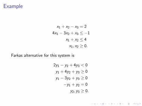
Example
x1 + x2 − x3 = 2
4x1 − 3x2 + x3 ≤ −1
x1 + x2 ≤ 4
x1, x2 ≥ 0.
Farkas alternative for this system is
2y1 − y2 + 4y3 < 0
y1 + 4y2 + y3 ≥ 0
y1 − 3y2 + y3 ≥ 0
−y1 + y2 = 0
y2, y3 ≥ 0.
Example
x1 + x2 − x3 = 2
4x1 − 3x2 + x3 ≤ −1
x1 + x2 ≤ 4
x1, x2 ≥ 0.
Farkas alternative for this system is
2y1 − y2 + 4y3 < 0
y1 + 4y2 + y3 ≥ 0
y1 − 3y2 + y3 ≥ 0
−y1 + y2 = 0
y2, y3 ≥ 0.
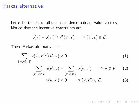
Farkas alternative
Let E be the set of all distinct ordered pairs of value vectors.Notice that the incentive constraints are:
p(v)− p(v ′) ≤ `f (v ′, v) ∀ (v ′, v) ∈ E .
Then, Farkas alternative is:∑(v ′,v)∈E
x(v ′, v)`f (v ′, v) < 0 (1)
∑(v ′,v)∈E
x(v ′, v) =∑
(v ,v ′)∈E
x(v , v ′) ∀ v ∈ V (2)
x(v , v ′) ≥ 0 ∀ (v , v ′) ∈ E . (3)

Illustration
Suppose V = {v1, v2, v3}. Then, incentive constraints are:
p(v1)− p(v2) ≤ `f (v2, v1)
p(v1)− p(v3) ≤ `f (v3, v1)
p(v2)− p(v1) ≤ `f (v1, v2)
p(v2)− p(v3) ≤ `f (v3, v2)
p(v3)− p(v1) ≤ `f (v1, v3)
p(v2)− p(v2) ≤ `f (v2, v3).
Illustration
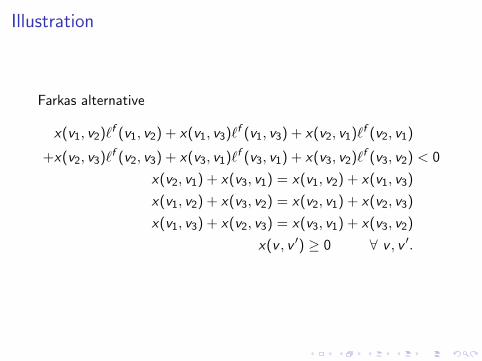
Farkas alternative
x(v1, v2)`f (v1, v2) + x(v1, v3)`f (v1, v3) + x(v2, v1)`f (v2, v1)
+x(v2, v3)`f (v2, v3) + x(v3, v1)`f (v3, v1) + x(v3, v2)`f (v3, v2) < 0
x(v2, v1) + x(v3, v1) = x(v1, v2) + x(v1, v3)
x(v1, v2) + x(v3, v2) = x(v2, v1) + x(v2, v3)
x(v1, v3) + x(v2, v3) = x(v3, v1) + x(v3, v2)
x(v , v ′) ≥ 0 ∀ v , v ′.

Flow interpretation of dual variables
v_3
−2
2
3
−1
0
1
v_1
v_2
Interpreting Farkas alternative
I Variable x(v , v ′) is the flow in the edge (v , v ′) (i.e., in theedge from v to v ′).
I So, the second (equality) set of constraints (2) in the Farkasalternative says
I the total flow into a node must equal the total flow out of it.I This is a feasible flow constraint.
I Call any x which satisfies constraints (2) and (3) a feasibleflow.
Flow decomposition
I Consider a feasible flow x and an edge (v , v ′).
I Let C (v , v ′) be the set of cycles through edge (v , v ′).
I Fact: For any feasible flow x we can define flows x(C ) foreach cycle C in graph G f such that
x(v , v ′) =∑
C∈C(v ,v ′)
x(C ).

Illustration of flow decomposition
v_2
10
7
2
1
4
5
v_1
v_3
Figure: A feasible flow

Illustration of flow decomposition continued
v_2
104
5
0 6
1
v_1
v_3
Figure: Flows for cycles

Illustration of flow decomposition continued
v_3
10
0 6
0
4
4
v_1
v_2
Figure: Flows for cycles
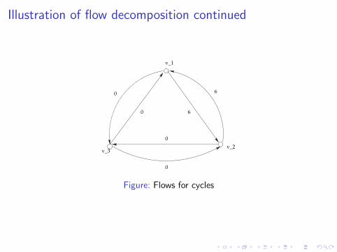
Illustration of flow decomposition continued
v_3
0 6
0
0
0
6
v_1
v_2
Figure: Flows for cycles

Illustration of flow decomposition continued
v_3
0
0
0
0
0
0
v_1
v_2
Figure: Flows for cycles
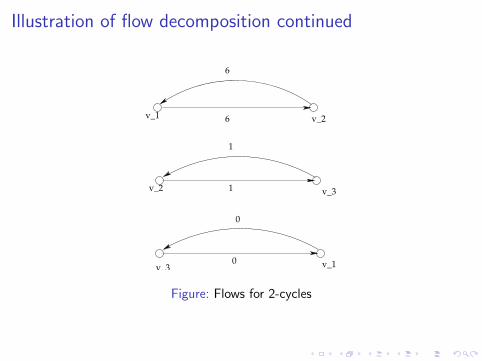
Illustration of flow decomposition continued
v_1
1
1
6
6
0
0
v_1 v_2
v_2 v_3
v_3
Figure: Flows for 2-cycles

Illustration of flow decomposition continued
v_3
1 1
1
44
4
v_1
v_2
v_3
v_1
v_2
Figure: Flows for 3-cycles

Back to Farkas alternative
I Constraint (1) says that the weighted sum of flows must benegative.
I Using `f (C ) to denote the length of a cycle C , we get∑(v ′,v)∈E
x(v ′, v)`f (v ′, v) =∑
(v ′,v)∈E
∑C∈C(v ′,v)
x(C )`f (v ′, v)
=∑C
∑(v ′,v)∈C
x(C )`f (v ′, v)
=∑C
x(C )`f (C ).

Proof of Theorem
I Suppose every cycle in G f has non-negative length.
I Since each flow is non-negative,∑
C x(C )`f (C ) ≥ 0.
I Hence, Farkas alternative has no solution.
I So, f can be truthfully implemented.

Proof of Theorem
If f can be implemented trutfully, then the Farkas alternative musthave no solution.
So, for every feasible flow x , we must have∑
C x(C )`f (C ) ≥ 0.
I Suppose cycle C ∗ has negative length.
I Then define a feasible flow which flows one unit along C ∗ andzero elsewhere.
I Then∑
C x(C )`f (C ) = `f (C ∗) < 0.
I Hence, the Farkas alternative has a solution, a contradiction.