graphical approach to college algebra 6th edition hornsby ... · section 2.1 69 copyright © 2015...
TRANSCRIPT

Section 2.1 69
Copyright © 2015 Pearson Education, Inc
Chapter 2: Analysis of Graphs and Functions
2.1: Graphs of Basic Functions and Relations; Symmetry
1. ( , ).
2. ( , ); [0, )
3. (0,0)
4. [0, ); [0, )
5. increases
6. ( ,0]; [0, )
7. x-axis
8. even
9. odd
10. y-axis; origin
11. The domain can be all real numbers; therefore, the function is continuous for the interval ( , ) .
12. The domain can be all real numbers; therefore, the function is continuous for the interval ( , ) .
13. The domain can only be values where 0;x therefore, the function is continuous for the interval [0, ).
14. The domain can only be values where 0;x therefore, the function is continuous for the interval ( ,0].
15. The domain can be all real numbers except 3; therefore, the function is continuous for the interval
( , 3) ( 3, ).
16. The domain can be all real numbers except 1; therefore, the function is continuous for the
interval ( ,1) (1, ).
17. (a) The function is increasing for the interval 3,
(b) The function is decreasing for the interval ,3
(c) The function is never constant; therefore, none.
(d) The domain can be all real numbers; therefore, the interval ( , ).
(e) The range can only be values where 0;y therefore, the interval [0, ).
18. (a) The function is increasing for the interval 4,
(b) The function is decreasing for the interval , 1
(c) The function is constant for the interval 1,4
(d) The domain can be all real numbers; therefore, the interval ( , ).
(e) The range can only be values where 3;y therefore, the interval [3, ).
19. (a) The function is increasing for the interval ,1
(b) The function is decreasing for the interval 4,
Graphical Approach to College Algebra 6th Edition Hornsby Solutions ManualFull Download: http://testbanklive.com/download/graphical-approach-to-college-algebra-6th-edition-hornsby-solutions-manual/
Full download all chapters instantly please go to Solutions Manual, Test Bank site: testbanklive.com

70 Chapter 2: Analysis of Graphs of Functions
Copyright © 2015 Pearson Education, Inc
(c) The function is constant for the interval 1,4
(d) The domain can be all real numbers; therefore, the interval ( , ).
(e) The range can only be values where 3;y therefore, the interval ( ,3].
20. (a) The function is never increasing; therefore, none.
(b) The function is always decreasing; therefore, the interval ( , ).
(c) The function is never constant; therefore, none.
(d) The domain can be all real numbers; therefore, the interval ( , ).
(e) The range can be all real numbers; therefore, the interval ( , ).
21. (a) The function is never increasing; therefore, none
(b) The function is decreasing for the intervals , 2 and 3,
(c) The function is constant for the interval ( 2,3).
(d) The domain can be all real numbers; therefore, the interval ( , ).
(e) The range can only be values where 1.5y or 2;y therefore, the interval ( ,1.5] [2, ).
22. (a) The function is increasing for the interval (3, ).
(b) The function is decreasing for the interval ( , 3).
(c) The function is constant for the interval 3,3
(d) The domain can be all real numbers except 3; therefore, the interval ( , 3) ( 3, ).
(e) The range can only be values where 1;y therefore, the interval (1, ).
23. Graph 5( ) .f x x See Figure 23. As x increases for the interval ( , ), y increases; therefore, the
function is increasing.
24. Graph 3( ) .f x x See Figure 24. As x increases for the interval ( , ), y decreases; therefore, the
function is decreasing.
25. Graph 4( ) .f x x See Figure 25. As x increases for the interval ,0 y decreases; therefore, the
function is decreasing on ,0
26. Graph 4( ) .f x x See Figure 26. As x increases for the interval 0, , y increases; therefore, the function
is increasing on 0,
[-10,10] by [-10,10] [-10,10] by [-10,10] [-10,10] by [-10,10] [-10,10] by [-10,10] Xscl = 1 Yscl = 1 Xscl = 1 Yscl = 1 Xscl= 1 Yscl = 1 Xscl = 1 Yscl= 1
Figure 23 Figure 24 Figure 25 Figure 26

Section 2.1 71
Copyright © 2015 Pearson Education, Inc
27. Graph ( ) | | .f x x See Figure 27. As x increases for the interval ,0 , y increases; therefore, the
function is increasing on ,0 .
28. Graph ( ) | | .f x x See Figure 28. As x increases for the interval 0, , y decreases; therefore, the
function is decreasing on 0, .
29. Graph 3( ) .f x x See Figure 29. As x increases for the interval ( , ), y decreases; therefore, the
function is decreasing.
30. Graph ( ) .f x x See Figure 30. As x increases for the interval 0, y decreases; therefore, the
function is decreasing.
[-10,10] by [-10,10] [-10,10] by [-10,10] [-10,10] by [-10,10] [-10,10] by [-10,10]
Xscl = 1 Yscl = 1 Xscl = 1 Yscl = 1 Xscl= 1 Yscl = 1 Xscl = 1 Yscl= 1
Figure 27 Figure 28 Figure 29 Figure 30
31. Graph 3( ) 1 .f x x See Figure 31. As x increases for the interval ( , ), y decreases; therefore, the function is
decreasing.
32. Graph 2( ) 2 .f x x x See Figure 32. As x increases for the interval 1, y increases; therefore, the
function is increasing on 1, .
33. Graph 2( ) 2 .f x x See Figure 33. As x increases for the interval ,0 y increases; therefore, the
function is increasing on ,0 .
34. Graph ( ) | 1 | .f x x See Figure 34. As x increases for the interval , 1 y decreases; therefore, the
function is decreasing on , 1 .
[-10,10] by [-10,10] [-10,10] by [-10,10] [-10,10] by [-10,10] [-10,10] by [-10,10]
Xscl = 1 Yscl = 1 Xscl = 1 Yscl = 1 Xscl= 1 Yscl = 1 Xscl = 1 Yscl= 1
Figure 31 Figure 32 Figure 33 Figure 34

72 Chapter 2: Analysis of Graphs of Functions
Copyright © 2015 Pearson Education, Inc
35. (a) No (b) Yes (c) No
36. (a) Yes (b) No (c) No
37. (a) Yes (b) No (c) No
38. (a) No (b) No (c) Yes
39. (a) Yes (b) Yes (c) Yes
40. (a) Yes (b) Yes (c) Yes
41. (a) No (b) No (c) Yes
42. (a) No (b) Yes (c) No 43. (a) Since ( ) ( ),f x f x this is an even function and is symmetric with respect to the y-axis.
See Figure 43a. (b) Since ( ) ( ),f x f x this is an odd function and is symmetric with respect to the origin.
See Figure 43b.
Figure 43a Figure 43b
44. (a) Since this is an odd function and is symmetric with respect to the origin. See Figure 44a.
(b) Since this is an even function and is symmetric with respect to the y-axis. See Figure 44b
Figure 44a Figure 44b
45. If f is an even function then ( ) ( )f x f x or opposite domains have the same range. See Figure 45
46. If g is an odd function then ( ) ( )g x g x or opposite domains have the opposite range. See Figure 46
Figure 45 Figure 46
Section 2.1 73
Copyright © 2015 Pearson Education, Inc
47. This is an even function since opposite domains have the same range.
48. This is an even function since opposite domains have the same range.
49. This is an odd function since opposite domains have the opposite range.
50. This is an odd function since opposite domains have the opposite range.
51. This is neither even nor odd since the opposite domains are neither the opposite or same range.
52. This is neither even nor odd since the opposite domains are neither the opposite or same range.
53. If 4 2( ) 7 6,f x x x then 4 2 4 2( ) ( ) 7( ) 6 ( ) 7 6.f x x x f x x x ⇒ Since
( ) ( ),f x f x the function is even.
54. If 6 2( ) 2 8 ,f x x x then 6 2 6 2( ) 2( ) 8( ) ( ) 2 8 .f x x x f x x x ⇒ Since
( ) ( ),f x f x the function is even.
55. If 3( ) 3 ,f x x x then 3 3( ) 3( ) ( ) ( ) 3f x x x f x x x ⇒ and
3 3( ) (3 ) ( ) 3 .f x x x f x x x ⇒ Since ( ) ( ),f x f x the function is odd.
56. If 5 3( ) 2 3 ,f x x x x then 5 3 5 3( ) ( ) 2( ) 3( ) ( ) 2 3f x x x x f x x x x ⇒ and
5 3 5 3( ) ( 2 3 ) ( ) 2 3 .f x x x x f x x x x ⇒ Since ( ) ( ),f x f x the function is odd.
57. If 6 4( ) 4 5f x x x then 6 4 6 4( ) ( ) 4( ) 5 ( ) 4 5.f x x x f x x x ⇒ Since
( ) ( ),f x f x the function is even.
58. If ( ) 8,f x then ( ) 8.f x Since ( ) ( ),f x f x the function is even.
59. If 5 3( ) 3 7 ,f x x x x then 5 3 5 3( ) 3( ) ( ) 7( ) ( ) 3 7f x x x x f x x x x ⇒ and
5 3 5 3( ) (3 7 ) ( ) 3 7 .f x x x x f x x x x ⇒ Since ( ) ( ),f x f x the function is odd.
60. If 3( ) 4 ,f x x x then 3 3( ) ( ) 4( ) ( ) 4f x x x f x x x ⇒ and
3 3( ) ( 4 ) ( ) 4 .f x x x f x x x ⇒ Since ( ) ( ),f x f x the function is odd.
61. If ( ) | 5 |,f x x then ( ) | 5( ) | ( ) | 5 | .f x x f x x ⇒ Since ( ) ( ),f x f x the function is even.
62. If 2( ) 1,f x x then 2 2( ) ( ) 1 ( ) 1.f x x f x x Since ( ) ( ),f x f x the function is
even.
63. If ( 3,11)and (2,9) then 1 1
( ) ( )2( ) 2
f x f xx x
⇒
and 1 1
( ) ( )2 2
f x f xx x
⎛ ⎞ ⇒ ⎜ ⎟⎝ ⎠
Since
( ) ( ),f x f x the function is odd.
64. If 1
( ) 4 ,f x xx
then 1 1
( ) 4( ) ( ) 4( )
f x x f x xx x
⇒
and
1 1
( ) 4 ( ) 4 .f x x f x xx x
⎛ ⎞ ⇒ ⎜ ⎟⎝ ⎠
Since ( ) ( ),f x f x the function is odd.
65. If 3( ) 2 ,f x x x then 3 3( ) ( ) 2( ) ( ) 2f x x x f x x x ⇒ and

74 Chapter 2: Analysis of Graphs of Functions
Copyright © 2015 Pearson Education, Inc
3 3( ) ( 2 ) ( ) 2 .f x x x f x x x ⇒ Since ( ) ( ),f x f x the function is symmetric with
respect to the origin. Graph 3( ) 2 ;f x x x the graph supports symmetry with respect to the origin.
66. If 5 3( ) 2 ,f x x x then 5 3 5 3( ) ( ) 2( ) ( ) 2f x x x f x x x ⇒ and
5 3 5 3( ) ( 2 ) ( ) 2 .f x x x f x x x ⇒ Since ( ) ( ),f x f x the function is symmetric with
respect to the origin. Graph 5 3( ) 2 ;f x x x the graph supports symmetry with respect to the origin.
67. If 4 2( ) 0.5 2 1,f x x x then 4 2 4 2( ) 0.5( ) 2( ) 1 ( ) 0.5 2 1.f x x x f x x x ⇒
Since ( ) ( ),f x f x the function is symmetric with respect to the y-axis. Graph
4 2( ) 0.5 2 1;f x x x the graph supports symmetry with respect to the y-axis.
68. If 2( ) 0.75 | | 1,f x x x then 2 2( ) 0.75( ) | ( ) | 1 ( ) 0.75 | | 1.f x x x f x x x ⇒
Since ( ) ( ),f x f x the function is symmetric with respect to the y-axis. Graph
4( ) .75 | | 1;f x x x the graph supports symmetry with respect to the y-axis.
69. If 3( ) 3,f x x x then 3 3( ) ( ) ( ) 3 ( ) 3f x x x f x x x ⇒ and
3 3( ) ( 3) ( ) 3.f x x x f x x x ⇒ Since ( ) ( ) ( ),f x f x f x the function is not
symmetric with respect to the y-axis or the origin.
70. If 4( ) 5 2,f x x x then 4 4( ) ( ) 5( ) 2 ( ) 5 2f x x x f x x x ⇒ and
4 4( ) ( 5 2) ( ) 5 2.f x x x f x x x ⇒ Since ( ) ( ) ( ),f x f x f x the function is
not symmetric with respect to the y-axis or the origin. Graph 4( ) 5 2;f x x x the graph supports no
symmetry with respect to the y-axis or the origin.
71. If 6 3( ) 4 ,f x x x then 6 3 6 3( ) ( ) 4( ) ( ) 4f x x x f x x x ⇒ and
6 3 6 3( ) ( 4 ) ( ) 4 .f x x x f x x x ⇒ Since ( ) ( ) ( ),f x f x f x the function is not
symmetric with respect to the y-axis or the origin. Graph 6 3( ) 4 ;f x x x the graph supports no
symmetry with respect to the y-axis or the origin.
72. If 3( ) 3 ,f x x x then 3 3( ) ( ) 3( ) ( ) 3f x x x f x x x ⇒ and
3 3( ) ( 3 ) ( ) 3 .f x x x f x x x ⇒ Since ( ) ( ),f x f x the function is symmetric with
respect to the origin. Graph 3( ) 3 ;f x x x the graph supports symmetry with respect to the origin.
73. If ( ) 6,f x then ( ) 6,f x Since ( ) ( ),f x f x the function is symmetric with respect to the y-
axis. Graph ( ) 6;f x the graph supports symmetry with respect to the y-axis.
74. If ( ) | |,f x x then ( ) | ( ) | ( ) | | .f x x f x x ⇒ Since ( ) ( ),f x f x the function is symmetric
with respect to the y-axis. Graph ( ) | |;f x x the graph supports symmetry with respect to the y-axis.

Section 2.2 75
Copyright © 2015 Pearson Education, Inc
75. If 3
1( ) ,
4f x
x then
3 3
1 1( ) ( )
4( ) 4f x f x
x x ⇒
and
3 3
1 1( ) ( ) .
4 4f x f x
x x⎛ ⎞ ⇒ ⎜ ⎟⎝ ⎠
Since
( ) ( ),f x f x the function is symmetric with respect to the origin. Graph3
1( ) ;
4f x
x the graph
supports symmetry with respect to the origin.
76. If 2( ) ( ) ,f x x f x x ⇒ then 2 2( ) ( ) ( ) ( ) .f x x f x x f x x ⇒ ⇒ Since
( ) ( ),f x f x the function is symmetric with respect to the y-axis. Graph 2( ) ;f x x the graph
2.2: Vertical and Horizontal Shifts of Graphs
1. The equation 2y x shifted 3 units upward is 2 3.y x
2. The equation 3y x shifted 2 units downward is 3 2.y x
3. The equation y x shifted 4 units downward is 4.y x
4. The equation 3y x shifted 6 units upward is 3 6.y x
5. The equation | |y x shifted 4 units to the right is | 4 | .y x
6. The equation | |y x shifted 3 units to the left is | 3 | .y x
7. The equation 3y x shifted 7 units to the left is 3( 7) .y x
8. The equation y x shifted 9 units to the right is 9.y x
9. The equation 2y x shifted 2 units downward and 3 units right is 23 2.y x
10. The equation 2y x shifted 4 units upward and 1 unit left is 21 4.y x
11. The equation y x shifted 3 units upward and 6 units to the left is 6 3.y x
12. The equation | |y x shifted 1 unit downward and 5 units to the right is | 5 | 1.y x
13. The equation 2y x shifted 500 units upward and 2000 units right is 22000 500.y x
14. The equation 2y x shifted 255 units downward and 1000 units left is 21000 255.y x
15. Shift the graph of f 4 units upward to obtain the graph of g.
16. Shift the graph of f 4 units to the left to obtain the graph of g.
17. The equation 2 3y x is 2y x shifted 3 units downward; therefore, graph B.
18. The equation 2( 3)y x is 2y x shifted 3 units to the right; therefore, graph C.
19. The equation 2( 3)y x is 2y x shifted 3 units to the left; therefore, graph A.
20. The equation | | 4y x is | |y x shifted 4 units upward; therefore; graph A.

76 Chapter 2: Analysis of Graphs of Functions
Copyright © 2015 Pearson Education, Inc
21. The equation | 4 | 3y x is | |y x shifted 4 units to the left and 3 units downward; therefore,
graph B.
22. The equation | 4 | 3y x is ( )y f x shifted 4 units to the right and 3 units downward; therefore,
graph C.
23. The equation 3( 3)y x is 3y x shifted 3 units to the right; therefore, graph C.
24. The equation 3( 2) 4y x is 3y x shifted 2 units to the right and 4 units downward; therefore,
graph A.
25. The equation 3( 2) 4y x is , .a b shifted 2 units to the left and 4 units downward; therefore,
graph B.
26. Using 2 1Y Y k and 0.x we get 19 15 4.k k ⇒
27. Using 2 1Y Y k and 0,x we get 5 3 2.k k ⇒
28. Using 2 1Y Y k and 0x , we get 5.5 4 1.5 1.5.k ⇒
29. From the graphs, (6,2) is a point on 1Y and (6, 1) a point on 2.Y Using 2 1Y Y k and 6,x we get
1 2 3.k k ⇒
30. From the graphs, ( 4,3) is a point on 1Y and ( 4,8) a point on 2.Y Using 2 1Y Y k and 4,x we
get 8 3 5.k k ⇒
31. For the equation 2 ,y x the Domain is ( , ) and the Range is [0, ). Shifting this 3 units downward
gives us: (a) Domain: ( , ) (b) Range: [ 3, ).
32. For the equation 2 ,y x the Domain is ( , ) and the Range is [0, ). Shifting this 3 units to the right
gives us: (a) Domain: ( , ) (b) Range: [0, ) .
33. For the equation | |,y x the Domain is ( , ) and the Range is [0, ). Shifting this 4 units to the left
and 3 units downward gives us: (a) Domain: ( , ) (b) Range: [ 3, ) .
34. For the equation | |,y x the Domain is ( , ) and the Range is [0, ). Shifting this 4 units to the
right and 3 units downward gives us: (a) Domain: ( , ) (b) Range: [ 3, ).
35. For the equation 3 ,y x the Domain is ( , ) and the Range is ( , ). Shifting this 3 units to the
right gives us: (a) Domain: ( , ) (b) Range: ( , )
36. For the equation 3 ,y x the Domain is ( , ) and the Range is ( , ) . Shifting this 2 units to the right
and 4 units downward gives us: (a) Domain: ( , ) (b) Range: ( , )
37. For the equation 2 ,y x the Domain is ( , ) and the Range is [0, ). Shifting this 1 unit to the right and
5 units downward gives us: (a) Domain: ( , ) (b) Range: [ 5, ) .
38. For the equation 2 ,y x the Domain is ( , ) and the Range is [0, ). Shifting this 8 units to the left and
3 units upward gives us: (a) Domain: ( , ) (b) Range: [3, ) .
39. For the equation ,y x the Domain is [0, ). and the Range is [0, ). Shifting this 4 units to the right
gives us: (a) Domain: [4, ). (b) Range: [0, ) .

Section 2.2 77
Copyright © 2015 Pearson Education, Inc
40. For the equation ,y x the Domain is [0, ). and the Range is [0, ). Shifting this 1 units to the left and
10 units downward gives us: (a) Domain: [ 1, ). (b) Range: [ 10, ) .
41. For the equation 3 ,y x the Domain is ( , ) and the Range is ( , ) . Shifting this 1 unit to the right
and 4 units upward gives us: (a) Domain: ( , ) (b) Range: ( , )
42. For the equation 3 ,y x the Domain is ( , ) and the Range is ( , ) . Shifting this 7 units to the left
and 10 units downward gives us: (a) Domain: ( , ) (b) Range: ( , )
43. The graph of ( )y f x is the graph of the equation 2y x shifted 1 unit to the right. See Figure 43.
44. The graph of 2y x is the graph of the equation y x shifted 2 units to the left. See Figure 44.
45. The graph of 3 1y x is the graph of the equation 3y x shifted 1 unit upward. See Figure 45.
Figure 43 Figure 44 Figure 45
46. The graph of | 2 |y x is the graph of the equation | |y x shifted 2 units to the left. See Figure 46.
47. The graph of 3( 1)y x is the graph of the equation 3y x shifted 1 unit to the right. See Figure 47.
48. The graph of | | 3y x is the graph of the equation | |y x shifted 3 units downward. See Figure 48.
Figure 46 Figure 47 Figure 48
49. The graph of 2 1y x is the graph of the equation y x shifted 2 units to the right and 1 unit
downward. See Figure 49.
50. The graph of 3 4y x is the graph of the equation y x shifted 3 units to the left and 4 units
downward. See Figure 50.
51. The graph of ( )f x is the graph of the equation 2y x shifted 2 units to the left and 3 units upward. See
Figure 51.

78 Chapter 2: Analysis of Graphs of Functions
Copyright © 2015 Pearson Education, Inc
Figure 49 Figure 50 Figure 51
52. The graph of 2( 4) 4y x is the graph of the equation 2y x shifted 4 units to the right and 4 units
downward. See Figure 52.
53. The graph of | 4 | 2y x is the graph of the equation | |y x shifted 4 units to the left and 2 units
downward. See Figure 53.
54. The graph of 3( 3) 1y x is the graph of the equation 3y x shifted 3 units to the left and 1 unit
downward. See Figure 54.
Figure 52 Figure 53 Figure 54
55. Since h and k are positive, the equation is 2y x shifted to the right and down; therefore, B.
56. Since h and k are positive, the equation is 2y x shifted to the left and down; therefore, D.
57. Since h and k are positive, the equation is 2y x shifted to the left and up; therefore, A.
58. Since h and k are positive, the equation is 2y x shifted to the right and up; therefore, C.
59. The equation ( ) 2y f x is ( )y f x shifted up 2 units or add 2 to the y-coordinate of each point as
follows: ( 3, 2) ( 3,0);( 1,4) ( 1,6);(5,0) (5,2). ⇒ ⇒ ⇒ See Figure 59.
60. The equation ( ) 2y f x is ( )y f x shifted down 2 units or subtract 2 from the y-coordinate of each
point as follows: ( 3, 2) ( 3, 4);( 1,4) ( 1,2);(5,0) (5, 2). ⇒ ⇒ ⇒ See Figure 60.

Section 2.2 79
Copyright © 2015 Pearson Education, Inc
Figure 59 Figure 60
61. The equation ( 2)y f x is ( )y f x shifted left 2 units or subtract 2 from the x-coordinate of each point
as follows: ( 3, 2) ( 5, 2);( 1,4) ( 3,4);(5,0) (3,0). ⇒ ⇒ ⇒ See Figure 61.
62. The equation ( 2)y f x is ( )y f x shifted right 2 units or add 2 to the x-coordinate of each point as
follows: ( 3, 2) ( 1, 2);( 1,4) (1, 4);(5,0) (7,0). ⇒ ⇒ ⇒ See Figure 62.
Figure 61 Figure 62 63. The graph is the basic function 2y x translated 4 units to the left and 3 units up; therefore, the new
equation is 2( 4) 3.y x The equation is now increasing for the interval: (a) 4, and decreasing for
the interval: (b) , 4 .
64. The graph is the basic function y x translated 5 units to the left; therefore, the new equation is 5.y x
The equation is now increasing for the interval: (a) 5, and does not decrease; therefore: (b) none.
65. The graph is the basic function 3y x translated 5 units down; therefore, the new equation is 3 5.y x
The equation is now increasing for the interval: (a) ( , ) and does not decrease; therefore: (b) none.
66. The graph is the basic function | |y x translated 10 units to the left; therefore, the new equation is
| 10 | .y x The equation is now increasing for the interval: (a) 10, and decreasing for the interval:
(b) , 10
67. The graph is the basic function y x translated 2 units to the right and 1 unit up; therefore, the new equation is
2 1.y x The equation is now increasing for the interval: (a) 2, and does not decrease; therefore: (b)
none.

80 Chapter 2: Analysis of Graphs of Functions
Copyright © 2015 Pearson Education, Inc
68. The graph is the basic function 2y x translated 2 units to the right and 3 units down; therefore, the new
equation is 2( 2) 3.y x The equation is now increasing for the interval: (a) 2, and decreasing for
the interval: (b) , 2 .
69. (a) ( ) 0 : {3,4}f x
(b) ( ) 0 :f x for the intervals ( ,3) (4, ).
(c) ( ) 0 :f x for the interval (3, 4).
70. (a) ( ) 0 : { 2}f x
(b) ( ) 0 :f x for the interval 2, .
(c) ( ) 0 :f x for the interval , 2 .
71. (a) ( ) 0 : { 4,5}f x
(b) ( ) 0 :f x for the intervals ( ] [ ), 4 5,-¥ - È ¥
(c) ( ) 0 :f x for the interval [ 4,5].
72. (a) ( ) 0 :f x never; therefore: .
(b) ( ) 0 :f x for the interval [1, ).
(c) ( ) 0 :f x never; therefore: .
73. The translation is 3 units to the left and 1 unit up; therefore, the new equation is | 3 | 1.y x The form
| | y x h k will equal | 3 | 1y x when: 3h and 1.k
74. The equation 2y x has a Domain: ( , ) and a Range: [0, ). After the translation the Domain is
still: ( , ) but now the Range is (38, ) , a positive or upward shift of 38 units. Therefore, the
horizontal shift can be any number of units, but the vertical shift is up 38. This makes h any real number
and 38.k
75. (a) (4) 66.25(4) 160 425B ; In 2010, 425,000 bankruptcies were filed.
(b) We will use the point (2006, 160) and the slope of 66.25 in the point slope form for the equation of a
line. 1 1( ) 160 66.25( 2006) 66.25( 2006) 160y y m x x y x y x
(c) 66.25(2010 2006) 160 66.25(4) 160 425y , In 2010, 425,000 bankruptcies were filed.
(d) 133 133
293 66.25( 2006) 160 133 66.25( 2006) 2006 200666.25 66.25
x x x x .
There will be 293 thousand bankruptcies in 2008.
76. (a) 3
(14) (14) 15 97
S ; In 2013, sales were $9 billion.

Section 2.2 81
Copyright © 2015 Pearson Education, Inc
(b) We will use the point (1999, 15) and the slope of 3
7 in the point slope form for the equation of a
line. 1 1
3 3( ) 15 ( 1999) ( 1999) 15
7 7y y m x x y x y x
(c) 3 3
(2013 1999) 15 (14) 15 97 7
y ; In 2013, sales were $9 billion.
(d) 3 3
12 ( 1999) 15 3 ( 1999) 7 1999 20067 7
x x x x
77. 2(2011) 13(2011 2006) 115 13(25) 115 440U ; The average U.S. household spent $440 on Apple
products in 2011.
78. The formula for ( )W x can be found by shifting 2( ) 13( 2006) 115U x x to the right 4 units.
2( ) 13( 2010) 115W x x ; 2( ) 13(2015 2010) 115 13(25) 115 440W x
In 2015, the average worldwide household spending on Apple products was $440, which equaled U.S.
spending 4 years earlier.
79. (a) Enter the year in 1L and enter tuition and fees in 2L . The year 2000 corresponds to 0x and so on.
The regression equation is 402.5 3460.y x
(b) Since 0x corresponds to 2000, the equation when the exact year is entered is
402.5( 2000) 3460y x
(c) 402.5(2009 2000) 3460 $7100y y ⇒
80. (a) Enter the year in 1L and enter the percent of women in the workforce in 2 .L The year 1970 corresponds
to 0x and so on. The regression equation is 0.40167 46.36.y x
(b) Since 0x corresponds to 1970, the equation when the exact year is entered is
0.40167 1970 46.36.y x
(c) 0.40167 2015 1970 46.36 64.4y y ⇒
81. See Figure 81.
Figure 81

82 Chapter 2: Analysis of Graphs of Functions
Copyright © 2015 Pearson Education, Inc
82. 2 ( 2) 4
23 1 2
m m ⇒
83. Using slope-intercept form yields: 1 1 12 2( 3) 2 2 6 2 4y x y x y x ⇒ ⇒
84. (1, 2 6) and (3, 2 6) (1, 4) ⇒ and (3,8)
85. 8 4 4
23 1 2
m m ⇒
86. Using slope-intercept form yields: 2 2 24 2( 1) 4 2 2 2 2y x y x y x ⇒ ⇒ .
87. Graph 1 2 4y x and 2 2 2y x See Figure 87. The graph 2y can be obtained by shifting the graph
of 1y upward 6 units. The constant 6, comes from the 6 we added to each y-value in Exercise 84.
[-10,10] by [-10,10] Xscl = 1 Yscl = 1
Figure 87
88. c; c; the same as; c; upward (or positive vertical)
2.3: Stretching, Shrinking, and Reflecting Graphs
1. The function 2y x vertically stretched by a factor of 2 is 22 .y x
2. The function 3y x vertically shrunk by a factor of 1
2 is 31
.2
y x
3. The function y x reflected across the y-axis is .y x
4. The function 3y x reflected across the x-axis is 3 .y x
5. The function y x vertically stretched by a factor of 3 and reflected across the x-axis is 3 .y x
6. The function y x vertically shrunk by a factor of 1
3 and reflected across the y-axis is
1.
3y x
7. The function 3y x vertically shrunk by a factor of 0.25 and reflected across the y-axis is 30.25( )y x
or 30.25 .y x
8. The function y x vertically shrunk by a factor of 0.2 and reflected across the x-axis is 0.2y x .
9. Graph 1y x , 2 3y x ( 1y shifted up 3 units), and 3 3y x ( 1y shifted down 3 units). See Figure 9.
10. Graph 31y x , 3
2 4y x ( 1y shifted up 4 units), and 33 4y x ( 1y shifted down units).
See Figure 10.
11. Graph 1y x , 2 3y x ( 1y shifted right 3 units), and 3 3y x ( 1y shifted left 3 units). See Figure 11.

Section 2.3 83
Copyright © 2015 Pearson Education, Inc
Figure 9 Figure 10 Figure 11 12. Graph 1 ,y x 2 3y x ( 1y shifted down 3 units), and 3 3y x ( 1y shifted up 3 units).
See Figure 12.
13. Graph 1 ,y x 2 6y x ( 1y shifted left 6 units), and 3 6y x ( 1y shifted right 6 units). See
Figure 13.
14. Graph 1y x , 2 2y x ( 1y stretched vertically by a factor of 2), and 3 2.5y x ( 1y stretched
vertically by a factor of 2.5). See Figure 14
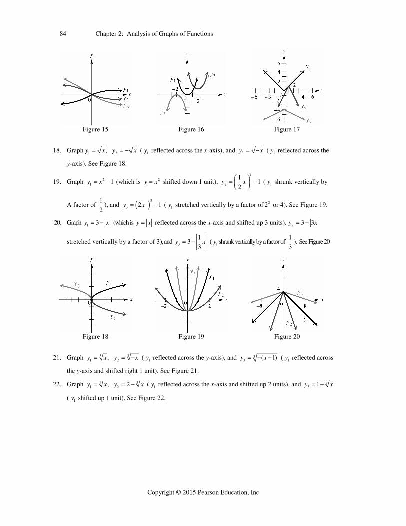
Figure 12 Figure 13 Figure 14 15. Graph 3
1 ,y x 32y x ( 1y reflected across the x-axis), and 3
3 2y x ( 1y reflected across the
x-axis and stretched vertically by a factor of 2). See Figure 15.
16. Graph 21 ,y x 2
2 ( 2) 1y x ( 1y shifted right 2 units and up 1 unit), and 23 ( 2)y x
( 1y shifted left 2 units and reflected across the x-axis). See Figure 16
17. Graph 1 ,y x 2 2 1 1y x ( 1y reflected across the x-axis, stretched vertically by a factor of 2,
shifted right 1 unit, and shifted up 1 unit), and 3
14
2y x ( 1y reflected across the x-axis, shrunk by
factor of 1
,2
and shifted down 4 units). See Figure 17
84 Chapter 2: Analysis of Graphs of Functions
Copyright © 2015 Pearson Education, Inc
Figure 15 Figure 16 Figure 17
18. Graph 1 ,y x 2y x ( 1y reflected across the x-axis), and 3y x ( 1y reflected across the
y-axis). See Figure 18.
19. Graph 21 1y x (which is 2y x shifted down 1 unit),
2
2
11
2y x
⎛ ⎞ ⎜ ⎟⎝ ⎠
( 1y shrunk vertically by
A factor of 1
2), and 2
3 2 1y x ( 1y stretched vertically by a factor of 22 or 4). See Figure 19.
20. Graph 1 3y x (which is y x reflected across the x-axis and shifted up 3 units), 2 3 3y x
stretched vertically by a factor of 3), and 3
13
3y x ( 1y shrunk vertically by a factor of
1
3). See Figure 20
Figure 18 Figure 19 Figure 20
21. Graph 31 ,y x 3
2y x ( 1y reflected across the y-axis), and 33 ( 1)y x ( 1y reflected across
the y-axis and shifted right 1 unit). See Figure 21.
22. Graph 31 ,y x 3
2 2y x ( 1y reflected across the x-axis and shifted up 2 units), and 33 1y x
( 1y shifted up 1 unit). See Figure 22.
Section 2.3 85
Copyright © 2015 Pearson Education, Inc
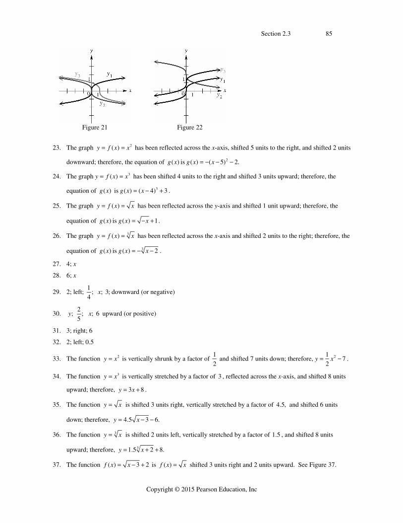
Figure 21 Figure 22
23. The graph 2( )y f x x has been reflected across the x-axis, shifted 5 units to the right, and shifted 2 units
downward; therefore, the equation of ( )g x is 2( ) ( 5) 2.g x x
24. The graph 3( )y f x x has been shifted 4 units to the right and shifted 3 units upward; therefore, the
equation of ( )g x is 3( ) ( 4) 3g x x .
25. The graph ( )y f x x has been reflected across the y-axis and shifted 1 unit upward; therefore, the
equation of ( )g x is ( ) 1g x x .
26. The graph 3( )y f x x has been reflected across the x-axis and shifted 2 units to the right; therefore, the
equation of ( )g x is 3( ) 2g x x .
27. 4; x
28. 6; x
29. 2; left; 1
;4
; 3;x downward (or negative)
30. 2
; ; ; 65
y x upward (or positive)
31. 3; right; 6
32. 2; left; 0.5
33. The function 2y x is vertically shrunk by a factor of 1
2 and shifted 7 units down; therefore, 21
72
y x .
34. The function 3y x is vertically stretched by a factor of 3 , reflected across the x-axis, and shifted 8 units
upward; therefore, 3 8y x .
35. The function y x is shifted 3 units right, vertically stretched by a factor of 4.5, and shifted 6 units
down; therefore, 4.5 3 6.y x
36. The function 3y x is shifted 2 units left, vertically stretched by a factor of 1.5 , and shifted 8 units
upward; therefore, 31.5 2 8.y x
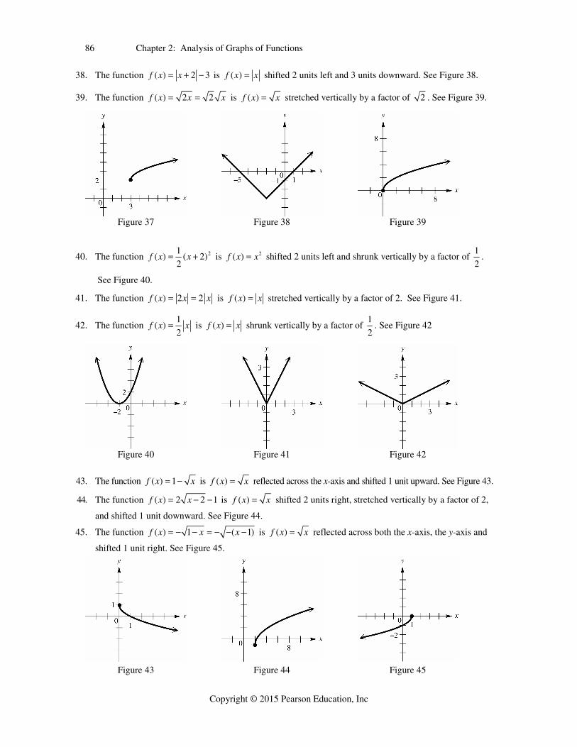
37. The function ( ) 3 2f x x is ( )f x x shifted 3 units right and 2 units upward. See Figure 37.
86 Chapter 2: Analysis of Graphs of Functions
Copyright © 2015 Pearson Education, Inc
38. The function ( ) 2 3f x x is ( )f x x shifted 2 units left and 3 units downward. See Figure 38.
39. The function ( ) 2 2f x x x is ( )f x x stretched vertically by a factor of 2 . See Figure 39.
Figure 37 Figure 38 Figure 39
40. The function 21( ) ( 2)
2f x x is 2( )f x x shifted 2 units left and shrunk vertically by a factor of
1
2.
See Figure 40.
41. The function ( ) 2 2f x x x is ( )f x x stretched vertically by a factor of 2. See Figure 41.
42. The function 1
( )2
f x x is ( )f x x shrunk vertically by a factor of 1
2. See Figure 42
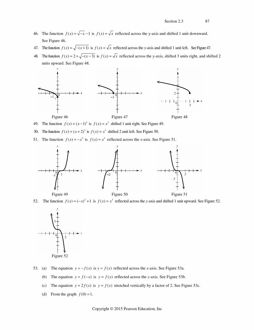
Figure 40 Figure 41 Figure 42 43. The function ( ) 1f x x is ( )f x x reflected across the x-axis and shifted 1 unit upward. See Figure 43.
44. The function ( ) 2 2 1f x x is ( )f x x shifted 2 units right, stretched vertically by a factor of 2,
and shifted 1 unit downward. See Figure 44.
45. The function ( ) 1 ( 1)f x x x is ( )f x x reflected across both the x-axis, the y-axis and
shifted 1 unit right. See Figure 45.
Figure 43 Figure 44 Figure 45
Section 2.3 87
Copyright © 2015 Pearson Education, Inc
46. The function ( ) 1f x x is ( )f x x reflected across the y-axis and shifted 1 unit downward.
See Figure 46.
47. The function ( ) ( 1)f x x is ( )f x x reflected across the y-axis and shifted 1 unit left. See Figure 47.
48. The function ( ) 2 ( 3)f x x is ( )f x x reflected across the y-axis, shifted 3 units right, and shifted 2
units upward. See Figure 48.
Figure 46 Figure 47 Figure 48 49. The function 3( ) ( 1)f x x is 3( )f x x shifted 1 unit right. See Figure 49.
50. The function 3( ) ( 2)f x x is 3( )f x x shifted 2 unit left. See Figure 50.
51. The function 3( )f x x is 3( )f x x reflected across the x-axis. See Figure 51.
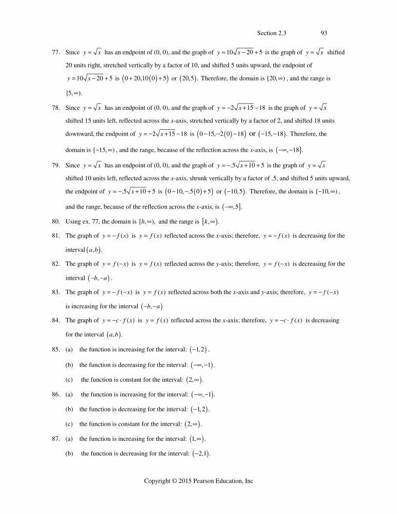
Figure 49 Figure 50 Figure 51 52. The function 3( ) ( ) 1f x x is 3( )f x x reflected across the y-axis and shifted 1 unit upward. See Figure 52.
Figure 52
53. (a) The equation ( )y f x is ( )y f x reflected across the x-axis. See Figure 53a.
(b) The equation ( )y f x is ( )y f x reflected across the y-axis. See Figure 53b.
(c) The equation 2 ( )y f x is ( )y f x stretched vertically by a factor of 2. See Figure 53c.
(d) From the graph (0) 1.f

88 Chapter 2: Analysis of Graphs of Functions
Copyright © 2015 Pearson Education, Inc
Figure 53a Figure 53b Figure 53c
54. (a) The equation ( )y f x is ( )y f x reflected across the x-axis. See Figure 54a.
(b) The equation ( )y f x is ( )y f x reflected across the y-axis. See Figure 54b.
(c) The equation 3 ( )y f x is ( )y f x stretched vertically by a factor of 3. See Figure 54c.
(d) From the graph (4) 1f
Figure 54a Figure 54b Figure 54c 55. (a) The equation ( )f x is ( )y f x reflected across the x-axis. See Figure 55a.
(b) The equation ( )y f x is ( )y f x reflected across the y-axis. See Figure 55b.
(c) The equation ( 1)y f x is ( )y f x shifted 1 unit to the left. See Figure 55c.
(d) From the graph, there are two x-intercepts, 1,0 and 4,0 .
Figure 55a Figure 55b Figure 55c
56. (a) The equation ( )y f x is ( )y f x reflected across the x-axis. See Figure 56a.
(b) The equation ( )y f x is ( )y f x reflected across the y-axis. See Figure 56b.
(c) The equation1
( )2
y f x is 20,5 . shrunk vertically by a factor of 1
.2
See Figure 56c.
(d) From the graph ( ) 0f x for the interval: ,0 .

Section 2.3 89
Copyright © 2015 Pearson Education, Inc
Figure 56a Figure 56b Figure 56c
57. (a) The equation ( )y f x is ( )y f x reflected across the x-axis. See Figure 57a.
(b) The equation 1
3y f x
⎛ ⎞ ⎜ ⎟⎝ ⎠
is ( )y f x stretched horizontally by a factor of 3. See Figure 57b.
(c) The equation 0.5 ( )y f x is ( )y f x shrunk vertically by a factor of 0.5. See Figure 57c.
(d) From the graph, symmetry with respect to the origin.
Figure 57a Figure 57b Figure 57c
58. (a) The equation (2 )y f x is ( )y f x stretched horizontally by a factor of1
2. See Figure 58a.
(b) The equation ( )y f x is ( )y f x reflected across the y-axis. See Figure 58b.
(c) The equation 3 ( )y f x is ( )y f x stretched vertically by a factor of 3. See Figure 58c.
(d) From the graph, symmetry with respect to the y-axis.
Figure 58a Figure 58b Figure 58c
59. (a) The equation ( ) 1y f x is ( )y f x shifted 1 unit upward. See Figure 59a.
(b) The equation 30 is ( )y f x reflected across the x-axis and shifted 1 unit down. See Figure 59b.

90 Chapter 2: Analysis of Graphs of Functions
Copyright © 2015 Pearson Education, Inc
(c) The equation1
22
y f x⎛ ⎞ ⎜ ⎟⎝ ⎠
is ( )y f x stretched vertically by a factor of 2 and horizontally by a
factor of 2. See Figure 59c.
Figure 59a Figure 59b Figure 59c
60. (a) The equation ( ) 2y f x is ( )y f x shifted 2 units downward. See Figure 60a.
(b) The equation ( 1) 2y f x is ( )y f x shifted 1 unit right and 2 units upward. See Figure 60b.
(c) The equation 2 ( )y f x is ( )y f x stretched vertically by a factor of 2. See Figure 60c.
Figure 60a Figure 60b Figure 60c
61. (a) The equation (2 ) 1y f x is x shrunk horizontally by a factor of 2 and shifted 1 unit upward.
See Figure 61a.
(b) The equation1
2 12
y f x⎛ ⎞ ⎜ ⎟⎝ ⎠
is ( )y f x stretched vertically by a factor of 2, stretched horizontally
by a factor of 2, and shifted 1 unit upward. See Figure 61b.
(c) The equation 1
( 2)2
y f x is ( )y f x shrunk vertically by a factor of 1
2 and shifted 2 units to the
right. See Figure 61c.
Figure 61a Figure 61b Figure 61c

Section 2.3 91
Copyright © 2015 Pearson Education, Inc
62. (a) The equation (2 )y f x is ( )y f x shrunk horizontally by a factor of1
2. See Figure 62a.
(b) The equation 11
2y f x
⎛ ⎞ ⎜ ⎟⎝ ⎠
is ( )y f x stretched horizontally by a factor of 2, and shifted 1 unit
downward. See Figure 62b.
(c) The equation 2 ( ) 1y f x is ( )y f x stretched vertically by a factor of 2 and shifted 1 unit
downward. See Figure 62c.
Figure 62a Figure 62b Figure 62c 63. (a) If (r, 0) is the x-intercept of ( )y f x and ( )y f x is ( )y f x reflected across the x-axis, then (r, 0)
is also the x-intercept of ( )y f x .
(b) If (r, 0) is the x-intercept of ( )y f x and ( )y f x is ( )f x reflected across the y-axis, then ,0r
is the x-intercept of ( )y f x
(c) If (r, 0) is the x-intercept of ( )y f x and ( )y f x is ( )y f x reflected across both the x-axis
and y-axis, then ,0 ,r is the x-intercept of ( )y f x .
64. (a) If (0, )b is the y-intercept of ( )y f x and ( )y f x is ( )y f x reflected across the x-axis,
then 0, b is the y-intercept of ( )y f x .
(b) If (0, )b is the y-intercept of ( )y f x and ( )y f x is ( )y f x reflected across the y-axis, then
(0, )b is also the y-intercept of ( )y f x .
(c) If (0, )b is the y-intercept of ( )y f x and 5 ( )y f x is ( )y f x stretched vertically by a factor of 5,
then (0,5 )b is the y-intercept of 5 ( )y f x .
(d) If (0, )b is the y-intercept of ( )y f x and 3 ( )y f x is ( )y f x reflected across the x-axis and
stretched vertically by a factor of 3, then (0, 3 )b is the y-intercept of 3 ( )y f x .
65. Since ( 2)y f x is ( )y f x shifted 2 units to the right, the domain of ( 2)f x is 1 2, 2 2
or 1,4 , and the range is the same: 0,3 .
66. Since 5 ( 1)f x is ( )f x shifted 1 unit to the left, the domain of 5 ( 1)f x is 1 1,2 1 or 2,1
and, stretched vertically by a factor of 5, the range is 5(0),5(3) or 0,15 .

92 Chapter 2: Analysis of Graphs of Functions
Copyright © 2015 Pearson Education, Inc
67. Since ( )f x is ( )f x reflected across the x-axis, the domain of ( )f x is the same: 1,2 , and the
range is 3,0 . .
68. Since ( 3) 1f x is ( )f x shifted 3 unit to the right, ( 3) 1f x is 1 3,2 3 or 2,5 , an
shifted 1 unit upward, the range is 0 1,3 1 or 1,4
69. Since (2 )f x is ( )f x shrunk horizontally by a factor of 1
2, the domain of (2 )f x is 1 1
( 1), (2)2 2⎡ ⎤⎢ ⎥⎣ ⎦
or 1
,12
⎡ ⎤⎢ ⎥⎣ ⎦, and the range is the same: 0,3 .
70. Since 2 ( 1)f x is ( )f x shifted 1 unit to the right, the domain of 2 ( 1)f x is 1 1,2 1 or
0,3 , and stretched vertically by a factor of 3, the range is 2( 2), 2(3) or 0,6 .
71. Since 1
34
f x⎛ ⎞⎜ ⎟⎝ ⎠
is ( )f x stretched horizontally by a factor of 4 , the domain of 1
34
f x⎛ ⎞⎜ ⎟⎝ ⎠
is 4( 1),4(2)
or 4,8 , and stretched vertically by a factor of 3, the range is 3(0),3(3) or 0,9 .
72. Since 2 (4 )f x is ( )f x shrunk horizontally by a factor of 1
4, the domain of 2 (4 )f x is
1 1( 1), (2)
4 4⎡ ⎤⎢ ⎥⎣ ⎦
or
1 1
, ;4 2
⎡ ⎤⎢ ⎥⎣ ⎦ and reflected across the x-axis while being stretched vertically by a factor of 2, the range is
2(0), 2(3) 0, 6 or 6,0 .
73. Since ( )f x is ( )f x reflected across the y-axis, the domain of ( )f x is ( 1), (2) 1, 2 or 2,1 ;
and the range is the same: 0,3 .
74. Since 2 ( )f x is ( )f x reflected across the y-axis, the domain of 2 ( )f x is ( 1), (2) 1, 2 or
2,1 , and reflected across the x-axis while being stretched vertically by a factor of 2, the range is
2(0), 2(3) 0, 6 or 6,0 .
75. Since ( 3 )f x is ( )f x reflected across the y-axis and shrunk horizontally by a factor of1
3, the domain of
( 3 )f x is 1 1 1 2
( 1), (2) ,3 3 3 3
⎡ ⎤ ⎡ ⎤ ⎢ ⎥ ⎢ ⎥⎣ ⎦ ⎣ ⎦ or
2 1,
3 3⎡ ⎤⎢ ⎥⎣ ⎦
, and the range is the same: 0,3 .
76. Since 1
( 3)3
f x is ( )f x shifted 3 units to the right, the domain of 1
( 3)3
f x is 1 3,2 3 or 2,5 ,
and shrunk vertically by a factor of 1
,3
the range is 1 10 , 3
3 3⎡ ⎤⎢ ⎥⎣ ⎦
or 0,1 .
Section 2.3 93
Copyright © 2015 Pearson Education, Inc
77. Since y x has an endpoint of (0, 0), and the graph of 10 20 5y x is the graph of y x shifted
20 units right, stretched vertically by a factor of 10, and shifted 5 units upward, the endpoint of
10 20 5y x is 0 20,10 0 5 or 20,5 . Therefore, the domain is [20, ) , and the range is
[5, ).
78. Since y x has an endpoint of (0, 0), and the graph of 2 15 18y x is the graph of y x
shifted 15 units left, reflected across the x-axis, stretched vertically by a factor of 2, and shifted 18 units
downward, the endpoint of 2 15 18y x is 0 15, 2 0 18 or 15, 18 . Therefore, the
domain is [ 15, ) , and the range, because of the reflection across the x-axis, is , 18 .
79. Since y x has an endpoint of (0, 0), and the graph of .5 10 5y x is the graph of y x
shifted 10 units left, reflected across the x-axis, shrunk vertically by a factor of .5, and shifted 5 units upward,
the endpoint of .5 10 5y x is 0 10, .5 0 5 or 10,5 . Therefore, the domain is [ 10, ) ,
and the range, because of the reflection across the x-axis, is ,5 .
80. Using ex. 77, the domain is [ , ),h and the range is , .k
81. The graph of ( )y f x is ( )y f x reflected across the x-axis; therefore, ( )y f x is decreasing for the
interval , .a b
82. The graph of ( )y f x is ( )y f x reflected across the y-axis; therefore, ( )y f x is decreasing for the
interval ,b a .
83. The graph of ( )y f x is ( )y f x reflected across both the x-axis and y-axis; therefore, ( )y f x
is increasing for the interval ,b a
84. The graph of ( )y c f x is ( )y f x reflected across the x-axis; therefore, ( )y c f x is decreasing
for the interval , .a b
85. (a) the function is increasing for the interval: 1,2 .
(b) the function is decreasing for the interval: , 1 .
(c) the function is constant for the interval: 2, .
86. (a) the function is increasing for the interval: , 1 .
(b) the function is decreasing for the interval: 1,2 .
(c) the function is constant for the interval: 2, .
87. (a) the function is increasing for the interval: 1, .
(b) the function is decreasing for the interval: 2,1 .

94 Chapter 2: Analysis of Graphs of Functions
Copyright © 2015 Pearson Education, Inc
(c) the function is constant for the interval: , 2 .
88. (a) the function is increasing for the interval: , 3 .
(b) the function is decreasing for the interval: 3, .
(c) the function is not constant for any interval.
89. From the graph, the point on 2y is approximately 8,10 .
90. From the graph, the point on 2y is approximately 27, 15 .
91. Use two points on the graph to find the slope. Two points are 2, 1 and 1,1 ; therefore, the slope is
1 1 22.
1 2 1m m
⇒
The stretch factor is 2 and the graph has been shifted 2 units to the left and 1
unit down; therefore, the equation is 2 2 1.y x
92. Use two points on the graph to find the slope. Two points are 1,2 and 5,0 ; therefore, the slope is
0 2 2 1
.5 1 4 2
m m ⇒
The shrinking factor is 1
,2
the graph has been reflected across the x-axis,
shifted 1 unit to the right, and shifted 2 units upward; therefore, the equation is 1
1 2.2
y x
93. Use two points on the graph to find the slope. Two points are 0,2 and 1, 1 ; therefore, the slope is
1 2 3
3.1 0 1
m m ⇒
The stretch factor is 3, the graph has been reflected across the x-axis, and
shifted 2 units upward; therefore, the equation is 3 2.y x
94. Use two points on the graph to find the slope. Two points are 1, 2 and 0,1 ; therefore, the slope is
1 2 33.
0 1 1m m
⇒
The stretch factor is 3 and the graph has been shifted 1 unit to the left and 2
units down; therefore, the equation is 3 1 2.y x
95. Use two points on the graph to find the slope. Two points are (0,-4) and (3,0); therefore, the slope is
4 0 4 4
.0 3 3 3
m m ⇒
The stretch factor is 4
3and the graph has been shifted 4 units down.; therefore,
the equation is 4
43
y x .
96. Use two points on the graph to find the slope. Two points are (0,4) and (-3,5); therefore, the slope is
5 4 1 1
.3 0 3 3
m m ⇒
The stretch factor is
1
3 and the graph has been shifted 3 units to the left and
5 units up.; therefore, the equation is 1
3 53
y x .

Section 2.3 95
Copyright © 2015 Pearson Education, Inc
97. Since ( )y f x is symmetric with respect to the y-axis, for every ( , )x y on the graph, ( , )x y is also on
the graph. Reflection across the y-axis reflect onto itself and will not change the graph. It will be the same.
Reviewing Basic Concepts (Sections 2.1—2.3)
1. (a) The function ( )f x x shifted up one unit yields the function ( ) 1f x x . Therefore, this function
has a domain of , and a range of of 1, . The function is increasing from 0, and
decreasing from ,0 .
(b) The function 2( )f x x shifted to the right 2 units yields the function 2( ) 2f x x . Therefore, this
function has a domain of , and a range of of 0, . The function is increasing from 2, and
decreasing from , 2 .
(c) The function ( )f x x reflected over the x-axis yields the function ( )f x x . Therefore, this
function has a domain of 0, and a range of of ,0 . The function is never increasing and
decreasing from 0, .
2. (a) If ( )y f x is symmetric with respect to the origin, then another function value is ( 3) 6.f
(b) If ( )y f x is symmetric with respect to the y-axis, then another function value is ( 3) 6.f
(c) If ( ) ( ), ( )f x f x y f x is symmetric with respect to both the x-axis and y-axis, then another
function value is ( 3) 6.f
(d) If ( ),y f x ( )y f x is symmetric with respect to the y-axis, then another function value is
( 3) 6.f
3. (a) The equation 27y x is 2y x shifted 7 units to the right: B.
(b) The equation 2 7y x is 2y x shifted 7 units downward: D.
(c) The equation 27y x is 2y x stretches vertically by a factor of 7: E.
(d) The equation 2( 7)y x is 2y x shifted 7 units to the left: A.
(e) The equation 2
1
3y x
⎛ ⎞ ⎜ ⎟⎝ ⎠
is 2y x stretches horizontally by a factor of 3: C.
4. (a) The equation 2 2y x is 2y x shifted 2 units upward: B.
(b) The equation 2 2y x is 2y x shifted 2 units downward: A.
(c) The equation 22y x is 2y x shifted 2 units to the left: G.
(d) The equation 2( 2)y x is 2y x shifted 2 units to the right: C.
(e) The equation 22y x is 2y x stretched vertically by a factor of 2: F.
(f) The equation 2y x is 2y x reflected across the x-axis D.
(g) The equation 22 1y x is 2y x shifted 2 units to the right and 1 unit upward: H.
(h) The equation 22 1y x is 2y x shifted 2 units to the left and 1 unit upward: E.

96 Chapter 2: Analysis of Graphs of Functions
Copyright © 2015 Pearson Education, Inc
5. (a) The equation 4y x is y x shifted 4 units upward. See Figure 5a.
(b) The equation 4y x is y x shifted 4 units to the left. See Figure 5b.
(c) The equation 4y x is y x shifted 4 units to the right. See Figure 5c.
(d) The equation 2 4y x is y x shifted 2 units to the left and 4 units down. See Figure 5d.
(e) The equation 2 4y x is y x reflected across the x-axis, shifted 2 units to the right, and 4
units upward. See Figure 5e.
Figure 5a Figure 5b Figure 5c
Figure 5d Figure 5e
6. (a) The graph is the function ( )f x x reflected across the x-axis, shifted 1 unit left and 3 units upward
Therefore, the equation is 1 3.y x
(b) The graph is the function ( )g x x reflected across the x-axis, shifted 4 units left and 2 units
upward. Therefore, the equation is 4 2.y x
(c) The graph is the function ( )g x x stretches vertically by a factor of 2, shifted 4 units left and 4
units downward. Therefore, the equation is 2 4 4.y x
(d) The graph is the function ( )f x x shrunk vertically by a factor of 1
,2
shifted 2 units right and 1
unit downward. Therefore, the equation is 1
2 1.2
y x
7. (a) The graph of ( )g x is the graph ( )f x shifted 2 units upward. Therefore, 2.c
(b) The graph of ( )g x is the graph ( )f x shifted 4 units to the left. Therefore, 4.c
8. The graph of y F x h is a horizontal translation of the graph of y F x . The graph of
y F x h is not the same as the graph of ,y F x h because the graph of y F x h is a
vertical translation of the graph of .y F x

Section 2.4 97
Copyright © 2015 Pearson Education, Inc
9. (a) If f is even, then ( ) ( ).f x f x See Figure 9a.
(b) If f is odd, then ( ) ( ).f x f x See Figure 9b.
Figure 9a Figure 9b
10. (a) ( ) 5(7) 2 37R x , In 2011, Google’s ad revenues were $37 billion.
(b) Using the point (2004, 2) and the slope of 5 with the point slope formula we will have
2 5( 2004) 5( 2004) 2y x y x .
(c) 5(2011 2004) 2 5(7) 2 37y , In 2011, Google’s ad revenues were $37 billion.
(d) 27 5( 2004) 2 25 5( 2004) 5 2004 2009x x x x
2.4: Absolute Value Functions
1. We reflect the graph of ( )y f x across the x-axis for all points for which 0.y Where 0,y the
graph remains unchanged. See Figure 1.
2. We reflect the graph of ( )y f x across the x-axis for all points for which 0.y Where 0,y the
graph remains unchanged. See Figure 2.
3. We reflect the graph of ( )y f x across the x-axis for all points for which 0.y Where 0,y the
graph remains unchanged. See Figure 3.
Figure 1 Figure 2 Figure 3
4. We reflect the graph of ( )y f x across the x-axis for all points for which 0.y Where 0,y the
graph remains unchanged. See Figure 4.
5. Since for all y, y 0, the graph remains unchanged. That is, ( )y f x has the same graph as ( ).y f x
6. We reflect the graph of ( )y f x across the x-axis for all points for which 0.y Where 0,y the
graph remains unchanged. See Figure 6.

98 Chapter 2: Analysis of Graphs of Functions
Copyright © 2015 Pearson Education, Inc
Figure 4 Figure 6
7. We reflect the graph of ( )y f x across the x-axis for all points for which 0.y Where 0,y the
graph remains unchanged. See Figure 7.
8. We reflect the graph of ( )y f x across the x-axis for all points for which 0.y Where 0,y the graph
remains unchanged. See Figure 8.
9. We reflect the graph of ( )y f x across the x-axis for all points for which 0.y Where 0,y the
graph remains unchanged. See Figure 9.
Figure 7 Figure 8 Figure 9 10. We reflect the graph of ( )y f x across the x-axis for all points for which 0.y Where 0,y the
graph remains unchanged.
11. If 5,f a then 5 5.f a
12. Since 2f x x is an even function, 2f x x and 2f x x are the same graph.
13. If 2 ,f x x then 2 2 .y f x y x y x ⇒ ⇒ Therefore, the range of y f x is [0,).
14. If the range of ( )y f x is [–2, ), the range of y f x is [0,) since all negative values of y are
reflected across the x-axis.
15. If the range of ( )y f x is , 2 , the range of ( )y f x is [2,) since all negative values of y are
reflected across the x-axis.
16. ( )f x is greater than or equal to 0 for any value of x. Since 1 is less than 0, –1 cannot be in the range of f

Section 2.4 99
Copyright © 2015 Pearson Education, Inc
17. From the graph of 2( 1) 2y x the domain of ( )f x is ( , ), and the range is [ 2, ).
From the graph of 21 2y x the domain of ( )f x is ( , ), and the range is [0, ).
18. From the graph of 1
22
y x the domain of ( )f x is ( , ), and the range is ( , ). From the
graph of 1
22
y x the domain of ( )f x is ( , ), and the range is [0, ).
19. From the graph of 21 2y x the domain of ( )f x is ( , ), and the range is ( , 1]. From
the graph of 21 2y x the domain of ( )f x is ( , ), and the range is [1, ).
20. From the graph of 2 2y x the domain of ( )f x is ( , ), and the range is ( , 2]. From
the graph of 2 2y x the domain of ( )f x is ( , ), and the range is [2, ).
21. From the graph, the domain of ( )f x is 2,3 , and the range is 2,3 . For the function ( ) ,y f x
we reflect the graph of ( )y f x across the x-axis for all points for which 0y , and, where 0,y the
graph remains unchanged. Therefore, the domain of ( )y f x is [–2, 3], and the range is [0, 3].
22. From the graph, the domain of ( )f x is [–3, 2], and the range is [–2, 2]. For the function ( ) ,y f x we
reflect the graph of ( )y f x across the x-axis for all points for which 0y and, where 0,y the graph
remains unchanged. Therefore, the domain of ( )y f x is [–3, 2], and the range is [0, 2].
23. From the graph, the domain of ( )f x is [–2, 3], and the range is [–3, 1]. For the function ( ) ,y f x we
reflect the graph of ( )y f x across the x-axis for all points for which 0y , and, where 0,y the graph
remains unchanged. Therefore, the domain of ( )y f x is [–2, 3], and the range is [0, 3].
24. From the graph, the domain of ( )y f x is [–3, 3], and the range is [–3, –1]. For the function ( ) ,y f x
we reflect the graph of ( )y f x across the x-axis for all points for which 0y , and, where 0,y the
graph remains unchanged. Therefore, the domain of ( )y f x is [–3, 3], and the range is [1, 3].
25. (a) The function ( )y f x is the function ( )y f x reflected across the y-axis. See Figure 25a.
(b) The function ( )y f x is the function ( )y f x reflected across both the x-axis and y-axis. See
Figure 25b.
(c) For the function ( )y f x we reflect the graph of ( )y f x (ex. b) across the x-axis for all
points for which 0y , and where 0,y the graph remains unchanged. See Figure 25c.

100 Chapter 2: Analysis of Graphs of Functions
Copyright © 2015 Pearson Education, Inc
Figure 25a Figure 25b Figure 25c
26. (a) The function ( )y f x is the function ( )y f x reflected across the y-axis. See Figure 26a.
(b) The function ( )y f x is the function ( )y f x reflected across both the x-axis and y-axis. See
Figure 26b
(c) For the function ( )y f x we reflect the graph of ( )y f x (ex. b) across the x-axis for all
points for which 0y , and, where 0,y the graph remains unchanged. See Figure 26c
Figure 26a Figure 26b Figure 26c
27. The graph of ( )y f x can not be below the x-axis; therefore, Figure A shows the graph of ( ),y f x
while Figure B shows the graph of ( ) .y f x
28. The graph of ( )y f x can not be below the x-axis; therefore, Figure B shows the graph of ( ),y f x
while Figure A shows the graph of ( ) .y f x
29. (a) From the graph, 1 2y y at the coordinates 1,5 and 6,5 ; therefore, the solution set is 1,6 .
(b) From the graph, 1 2y y for the interval 1,6 .
(c) From the graph, 1 2y y for the intervals , 1 6, .
30. (a) From the graph, 1 2y y at the coordinates 0, 2 and 8, 2 ; therefore, the solution set is 0,8 .
(b) From the graph, 1 2y y for the intervals ,0 8, .
(c) From the graph, 1 2y y for the interval 0,8 .
31 (a) From the graph, 1 2y y at the coordinate 4,1 ; therefore, the solution set is 4 .
(b) From the graph, 1 2y y never occurs; therefore, the solution set is .

Section 2.4 101
Copyright © 2015 Pearson Education, Inc
(c) From the graph, 1 2y y for all values for x except 4; therefore, the solution set is the intervals
, 4 4, .
32. (a) From the graph, 1 2y y never occurs; therefore, the solution set is .
(b) From the graph, 1 2y y for all values for x; therefore, the solution set is , .
(c). From the graph, 1 2y y never occurs; therefore, the solution set is .
33. The V-shaped graph is that of ( ) .5 6 ,f x x since this is typical of the graphs of absolute value functions
of the form ( ) | |f x ax b
34. The straight line graph is that of ( ) 3 14g x x which is a linear function.
35. The graphs intersect at 8,10 , so the solution set is 8 .
36. From the graph, ( ) ( )f x g x for the interval ,8 .
37. From the graph, ( ) ( )f x g x for the interval 8, .
38. If .5 6 3 14 0x x then .5 6 3 14.x x Therefore, the solution is the intersection of the graphs,
or 8 .
39. (a) 4 9 4 9x x ⇒ or 4 9 5x x ⇒ or 13.x The solution set is 13,5 , which is
supported by the graphs of 1 4y x and 2 9.y
(b) 4 9 4 9x x ⇒ or 4 9 5x x ⇒ or 13.x The solution is , 13 5, ,
which is supported by the graphs of 1 4y x and 2 9.y
(c) 4 9 9 4 9 13 5.x x x ⇒ ⇒ The solution is 13,5 , which is supported by the
graphs of | 4 |x and 2 9.y
40. (a) 3 5 3 5x x ⇒ or 3 5 8x x ⇒ or 2.x The solution set is 2,8 , which
supported by the graphs of 1 3y x and 2 5.y
(b) 3 5 3 5x x ⇒ or 3 5 8x x ⇒ or 2.x The solution is , 2 8, which is
supported by the graphs of 1 3y x and 2 5.y
(c) 3 5 5 3 5 2 8.x x x ⇒ ⇒ The solution is 2,8 , which is supported by the graphs
of 1 3y x and 2 5.y
41. (a) 7 2 3 7 2 3x x ⇒ or 7 2 3 2 4x x ⇒ or 2 10 2x x ⇒ or
5.x The solution set is 2,5 , which is supported by the graphs of 1 7 2y x and 2 3.y
(b) 7 2 3 7 2 3x x ⇒ or 7 2 3 2 4x x ⇒ or 2 10 2x x ⇒ or 5.x The
solution set is , 2 5, , which is supported by the graphs of 1 7 2y x and 2 3.y
102 Chapter 2: Analysis of Graphs of Functions
Copyright © 2015 Pearson Education, Inc
(c) 7 2 3 3 7 2 3 10 2 4 5 2x x x x ⇒ ⇒ ⇒ or 2 5.x The solution is 2,5 ,
which is supported by the graphs of 1 7 2y x and 2 3.y
42. (a) 9 3 6 9 3 6x x ⇒ or 9 3 6 3 15x x ⇒ or 3 3 5x x ⇒ or x = -1.
The solution set is 5, 1 , which is supported by the graphs of 1 9 3y x and 2 6.y
(b) 9 3 6 9 3 6x x ⇒ or 9 3 6 3 15x x ⇒ or 3 3 5x x ⇒ or 1.x
The solution is , 5 1, , which is supported by the graphs of 1 9 3y x and 2 6.y
(c) 9 3 6 6 9 3 6 3 3 15 1 5x x x x ⇒ ⇒ ⇒ or 5 1.x The solution is
5, 1 , which is supported by the graphs of 1 9 3y x and 2 6.y
43. (a) 2 1 3 5 2 1 2x x ⇒ or 2 1 2 2 1x x ⇒ or 1
2 32
x x ⇒ or 3
.2
x The
solution set is 3 1
, ,2 2
⎧ ⎫⎨ ⎬⎩ ⎭
which is supported by the graphs of 1 2 1 3y x and 2 5.y
(b) 3 1
2 1 3 5 2 2 1 2 3 2 1 .2 2
x x x x ⇒ ⇒ ⇒ The solution is 3 1
, ,2 2
⎡ ⎤⎢ ⎥⎣ ⎦ which is
supported by the graphs of 1 2 1 3y x and 2 5.y
(c) 2 1 3 5 2 1 2x x ⇒ or 2 1 2x ⇒ 2 1x or 1
2 32
x x ⇒ or 3
.2
x The solution
is 3 1
, , ,2 2
⎛ ⎤ ⎡ ⎞ ⎜ ⎟⎥ ⎢⎝ ⎦ ⎣ ⎠ which is supported by the graphs of 1 2 1 3y x and 2 5.y
44. (a) 7
4 7 4 4 4 7 0 4 7 .4
x x x x ⇒ ⇒ ⇒ The solution set is 7
,4
⎧ ⎫⎨ ⎬⎩ ⎭
which is supported
by the graphs of 1 4 7 4y x and 2 4.y
(b) 4 7 4 4 4 7 0x x ⇒ or 4 7 0 4 7x x ⇒ 7
4 74
x x ⇒ or 7
.4
x The
solution is 7 7
, , ,4 4
⎛ ⎞ ⎛ ⎞ ⎜ ⎟ ⎜ ⎟⎝ ⎠ ⎝ ⎠
which is supported by the graphs of 1 4 7 4y x and 2 4.y
(c) 7 7
4 7 4 4 0 4 7 0 7 4 74 4
x x x x ⇒ ⇒ ⇒ ⇒ the solution set is , which
is supported by the graphs of 1 4 7 4y x and 2 4.y
45. (a) 5
5 7 0 5 7 0 7 5 .7
x x x x ⇒ ⇒ ⇒ The solution set is 5
,7
⎧ ⎫⎨ ⎬⎩ ⎭
which is supported by the
graphs of 1 5 7y x and 2 0.y

Section 2.4 103
Copyright © 2015 Pearson Education, Inc
(b) 5 7 0 5 7 0x x ⇒ or 5 7 0 7 5x x ⇒ or 5
7 57
x x ⇒ or 5
.7
x The solution is
, , which is supported by the graphs of 1 5 7y x and 2 0.y
(c) 5 5
5 7 0 0 5 7 0 5 7 5 .7 7
x x x x ⇒ ⇒ ⇒ The solution set is 5
,7
⎧ ⎫⎨ ⎬⎩ ⎭
which is supported
by the graphs of 1 5 7y x and 2 0.y
46. (a) Absolute value is always positive; therefore, the solution set is , which is supported by the graphs of
1 8y x and 2 4.y
(b) Absolute value is always positive, and so cannot be less than 4; therefore, the solution set is ,
which is supported by the graphs of 1 8y x and 2 4.y
(c) Absolute value is always positive, and so is always greater than 4; therefore, the solution set is
, , which is supported by the graphs of 1 8y x and 2 4.y
47. (a) Absolute value is always positive; therefore, the solution set is , which is supported by the graphs of
1 2 3.6y x and 2 1.y
(b) Absolute value is always positive, and so cannot be less than or equal to 1; therefore, the solution set
is , which is supported by the graphs of 1 2 3.6y x and 2 1.y
(c) Absolute value is always positive, and so is always greater than 1; therefore, the solution is
, , which is supported by the graphs of 1 2 3.6y x and 2 1.y
48. 2 4 2 10 2 4 8 2 4 8x x x ⇒ ⇒ or 2 4 8 2 4x x ⇒ or 2 12 2x x ⇒ and
6.x Therefore, the solution set is 6,2 .
49. 3 4 3 4 8 3 4 3 12 4 3 4 4 3 4x x x x ⇒ ⇒ ⇒ or 4 3 4 3 0x x ⇒ or
3 8 0x x ⇒ or 8
.3
x Therefore, the solution set is 8
0, .3
⎧ ⎫⎨ ⎬⎩ ⎭
50. 5 3 2 18 5 3 20 3 4 3 4x x x x ⇒ ⇒ ⇒ or 3 4 1x x ⇒ or 7.x Therefore,
the solution set is 7,1 .
51. 1 1 3 1 3 1 3
2 2 22 2 4 2 2 2 2
x x x ⇒ ⇒ or 1 3
2 2 12 2
x x ⇒ or
1
2 22
x x ⇒ or 1.x Therefore, the solution set is 1
,1 .2
⎧ ⎫⎨ ⎬⎩ ⎭
52. 3 5 2 3 9 3 5 2 6 3 5 2 6x x x ⇒ ⇒ or 3 5 2 6 3 5 4x x ⇒ or
43 5 8 5
3x x ⇒ or
8 195
3 3x x ⇒ or
7.
3x Therefore, the solution set is
7 19, .
3 3⎧ ⎫⎨ ⎬⎩ ⎭

104 Chapter 2: Analysis of Graphs of Functions
Copyright © 2015 Pearson Education, Inc
53. 4.2 .5 1 3.1 4.2 .5 2.1 .5 .5 .5 .5x x x x ⇒ ⇒ ⇒ or .5 .5 0x x ⇒ or
1 0x x ⇒ or 1.x Therefore, the solution set is 0,1 .
54. 7
3 1 8 8 3 1 8 7 3 9 3.3
x x x x ⇒ ⇒ ⇒ Therefore, the solution is 7
,3 .3
⎛ ⎞⎜ ⎟⎝ ⎠
55. 15 7 7 15 7 22 8x x x ⇒ ⇒ or 8 22.x Therefore, the solution is 8,22 .
56. 7 4 11 11 7 4 11 18 4 4x x x ⇒ ⇒ ⇒9
1 .2
x Therefore, the solution is 9
1, .2
⎡ ⎤⎢ ⎥⎣ ⎦
57. 2 3 1 2 3 1x x ⇒ or 2 3 1 2 4x x ⇒ or 2
3( 3) 4 5( 3) .
9( 3)
f
g
⎛ ⎞ ⎜ ⎟ ⎝ ⎠ or 1.x Therefore,
the solution is ,1 2, .
58. 4 3 1 4 3 1x x ⇒ or 4 3 1 3 3x x ⇒ or 3 5 1x x ⇒ or 5
3x . Therefore, the solution is
5,1 ,
3⎛ ⎞ ⎜ ⎟⎝ ⎠
.
59. 3 8 3 3 8 3x x ⇒ or 3 8 3 3 5x x ⇒ or 53 11
3x x ⇒ or 11
.3
x
Therefore, the solution is 5 11, , .3 3
⎛ ⎤ ⎡ ⎞ ⎜ ⎟⎥ ⎢⎝ ⎦ ⎣ ⎠
60. Absolute value is always positive, and so is always greater than 1; therefore, the solution is , .
61. 1 16 0 6 0
3 3x x ⇒ or 1 1
6 0 63 3
x x ⇒ or 16 18
3x x ⇒ or 18.x Therefore,
the solution is every real number except 18: ,18 18, .
62. Absolute value is always positive, and cannot be less than 0; therefore, the solution set is . 63. Absolute value is always positive, and so cannot be less than or equal to 6; therefore, the solution set is .
64. Absolute value is always positive, and so cannot be less than 4; therefore, the solution set is .
65. Absolute value is always positive, and so is always greater than 5; therefore, the solution is , .
66. To solve such an equation, we must solve the compound equation ax b cx d or ax b cx d . The
solution set consists of the union of the two individual solution sets.
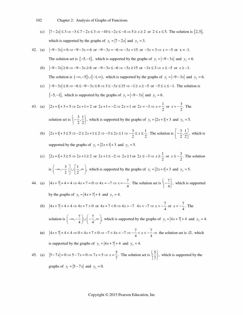
67. (a) 3 1 2 7 1 7 8x x x x ⇒ ⇒ 63 1 2 7 3 1 2 7 5 6 .
5x x x x x x ⇒ ⇒ ⇒
Therefore, the solution set is 6
8, .5
⎧ ⎫⎨ ⎬⎩ ⎭
(b) Graph 1 3 1y x and 2 2 7 .y x See Figure 67. From the graph, ( ) ( )f x g x when 1 2y y
which is for the interval 6, 8 , .
5⎛ ⎞ ⎜ ⎟⎝ ⎠
Section 2.4 105
Copyright © 2015 Pearson Education, Inc
(c) Graph 1 3 1y x and 2 2 7y x See Figure 67. From the graph, ( ) ( )f x g x when 1 2y y
which is for the interval 68, .
5⎛ ⎞⎜ ⎟⎝ ⎠
68. (a) 84 7 12 6 4 12 6 16
3x x x x x ⇒ ⇒ ⇒ or 4 7 12x x ⇒
4 7 12 8 4 12 8 8 1.x x x x x ⇒ ⇒ ⇒ Therefore, the solution set is 8, 1 .
3⎧ ⎫ ⎨ ⎬⎩ ⎭
(b) Graph 1 4y x and 2 7 12 .y x See Figure 68. From the graph, ( ) ( )f x g x when 1 2y y
which is for the interval 8, 1 .
3⎛ ⎞ ⎜ ⎟⎝ ⎠
(c) Graph 1 4y x and 2 7 12 .y x See Figure 68. From the graph, ( ) ( )f x g x when 1 2y y
which is for the interval 8, 1, .
3⎛ ⎞ ⎜ ⎟⎝ ⎠
[-20,20] by [-10,50] [-10,10] by [-4,16] Xscl = 2 Yscl = 5 Xscl = 1 Yscl = 1
Figure 67 Figure 68
69. (a) 2
2 5 3 3 23
x x x x ⇒ ⇒ or 2x +5= (x+3) ⇒ 2x +5 3x ⇒
8 8.x x ⇒ Therefore, the solution set is 2
,83
⎧ ⎫⎨ ⎬⎩ ⎭
.
(b) Graph 1 22 5 and y 3y x x . See Figure 69. From the graph, ( ) ( )f x g x when 1 2y y ,
which it is for the interval 2, 8,3
⎛ ⎞ ⎜ ⎟⎝ ⎠
.
(c) Graph 1 22 5 and y 3y x x . See Figure 69. From the graph, ( ) ( )f x g x when 1 2y y ,
which it is for the interval2
,83
⎛ ⎞⎜ ⎟⎝ ⎠
.
70. (a) 5
5 1 3 4 8 58
x x x x ⇒ ⇒ or 3
5x +1= (3 4) 5 1 3 4 2 32
x x x x x ⇒ ⇒ ⇒ .
Therefore, the solution set is 3 5
,2 8
⎧ ⎫⎨ ⎬⎩ ⎭
.
(b) Graph 1 5 1y x and 2 3 4 .y x See Figure 70. From the graph, ( ) ( )f x g x
when 1 2y y , which it is for the interval 3 5
, , .2 8
⎛ ⎞ ⎛ ⎞ ⎜ ⎟ ⎜ ⎟⎝ ⎠ ⎝ ⎠

106 Chapter 2: Analysis of Graphs of Functions
Copyright © 2015 Pearson Education, Inc
(c) Graph 1 5 1y x and 2 3 4y x . See Figure 70. From the graph, ( ) ( )f x g x when
1 2y y , which it is for the interval3 5
, .2 8
⎛ ⎞⎜ ⎟⎝ ⎠
[-10,10] by [-4,16] [-3,3] by [-4,16] [-6,6] by [-2,10] Xscl = 1 Yscl = 1 Xscl = 1 Yscl = 2 Xscl= 1 Yscl = 1
Figure 69 Figure 70 Figure 71
71. (a) 1 1 1 3
2 32 2 2 2
x x x x ⇒ ⇒ or 1 1
x 22 2
x⎛ ⎞ ⇒⎜ ⎟⎝ ⎠
1 12
2 2x x ⇒
3 5 5
2 2 3x x ⇒ . Therefore, the solution set is
53,
3⎧ ⎫⎨ ⎬⎩ ⎭
.
(b) Graph 1 2
1 1and 2
2 2y x y x . From the graph, ( ) ( )f x g x when 1 2y y , which it is for the
interval5
( , 3) , .3
⎛ ⎞ ⎜ ⎟⎝ ⎠
(c) Graph 1 2
1 1and y 2
2 2y x x .See Figure 71. From the graph ( ) ( )f x g x when 1 2y y ,
which it is for the interval 5
3,3
⎛ ⎞⎜ ⎟⎝ ⎠
.
72. (a) 1 2 153 8 5
3 3 2x x x x ⇒ ⇒ or 1 1
x +3= ( 8) 3 83 3
x x x ⇒ ⇒
4 3311
3 4x x ⇒ . Therefore, the solution set is 33 15
,4 2
⎧ ⎫⎨ ⎬⎩ ⎭
.
(b) Graph 1 3y x and 2
18
3y x . See Figure 72. From the graph, ( ) ( )f x g x when 1 2y y ,
which it is for the interval 33
,4
⎛ ⎞ ⎜ ⎟⎝ ⎠
15, .
2⎛ ⎞ ⎜ ⎟⎝ ⎠
(c) Graph 1 3y x and 2
18
3y x . See Figure 72. From the graph, ( ) ( )f x g x when 1 2y y ,
which it is for the interval 33 15
, .4 2
⎛ ⎞⎜ ⎟⎝ ⎠
73. (a) 4 1 4 6 1 6x x ⇒ ⇒ or 7
4 +1= (4 6) 4 1 4 6 8 7 .8
x x x x x ⇒ ⇒ ⇒
Therefore, the solution set is 7
8⎧ ⎫⎨ ⎬⎩ ⎭
.

Section 2.4 107
Copyright © 2015 Pearson Education, Inc
(b). Graph 1 4 1y x or 2y 4 6 .x See Figure 73. From the graph ( ) ( )f x g x when 1 2y y ,
which it is for the interval 7
,8
⎛ ⎞⎜ ⎟⎝ ⎠
.
(c) Graph 1 4 1y x or 2y 4 6 .x See Figure 73. From the graph, ( ) ( )f x g x when 1 2y y ,
which is for the interval 7
,8
⎛ ⎞ ⎜ ⎟⎝ ⎠
.
[-10,10] by [-10,10] [-10,10] by [-10,10] [-10,10] by [-10,10] Xscl = 1 Yscl = 1 Xscl = 1 Yscl = 1 Xscl= 1 Yscl = 1
Figure 72 Figure 73 Figure 74
74. (a) 6 9 6 3 9 3x x ⇒ ⇒ or 6 9 (6 9) 6 9 6 3x x x x ⇒ ⇒ 12 6x ⇒
6 16 .
12 2x ⇒ Therefore, the solution set is 1
2⎧ ⎫⎨ ⎬⎩ ⎭
.
(b) Graph 1 26 9 and 6 3y x y x . See Figure 74. From the graph, ( ) ( )f x g x when 1 2y y ,
which it is for the interval 1
, .2
⎛ ⎞ ⎜ ⎟⎝ ⎠
(c) Graph 1 26 9 and 6 3y x y x . See Figure 74. From the graph, ( ) ( )f x g x when 1 2y y ,
which it is for the interval 1
, .2
⎛ ⎞ ⎜ ⎟⎝ ⎠
75. (a) 0.25 1 0.75 3 0.50 4 8x x x x ⇒ ⇒ or 0.25 1 (0.75 3)x x ⇒ 0.25 1 0.75 3x x ⇒
2.x Therefore, the solution set is 2,8 .
(b) Graph 1 2.25 1 and .75 3 .y x y x See Figure 75. From the graph, ( ) ( )f x g x when 1 2y y ,
which it is for the interval (2,8).
(c) Graph 1 2.25 1 and .75 3 .y x y x See Figure 75. From the graph, ( ) ( )f x g x
when 1 2y y , which it is for the interval , 2 8, .
76. (a) .40 2 .60 5 20 7 35x x x x ⇒ ⇒ or .40 2 (.60 5)x x ⇒
.40 2 .60 5 3x x x ⇒ . Therefore, the solution set is 3,35 .
(b) Graph 1 2.40 2 and y .60 5y x x . See Figure 76. From the graph, ( ) ( )f x g x
when 1 2y y , which it is for the interval (3,35).

108 Chapter 2: Analysis of Graphs of Functions
Copyright © 2015 Pearson Education, Inc
(c ) Graph 1 2.40 2 and y .60 5y x x . See Figure 76. From the graph, ( ) ( )f x g x
when 1 2y y , which it is for the interval ,3 35, .
[-20,20] by [-4,16] [-30,50] by [-5,30] [-10,10] by [-10,10] [-10,10] by [-10,10] Xscl = 2 Yscl = 1 Xscl = 5 Yscl = 5 Xscl= 1 Yscl = 1 Xscl = 1 Yscl = 1
Figure 75 Figure 76 Figure 77 Figure 78
77. (a) 3 10 ( 3 10) 3 10 3 10x x x x ⇒ ⇒ there are an infinite number of solutions.
Therefore, the solution set is , .
(b) Graph 1 23 10 and y 3 10y x x . See Figure 77. From the graph, ( ) ( )f x g x
when 1 2y y , for which there is no solution.
(c ) Graph 1 23 10 and y 3 10y x x . See Figure 77. From the graph, ( ) ( )f x g x
when 1 2y y , for which there is no solution.
78. (a) 5 6 ( 5 6) 5 6 5 6x x x x ⇒ ⇒ there are an infinite number of solutions.
Therefore, the solution set is , .
(b) Graph 1 25 6 and y 5 6y x x . See Figure 78. From the graph, ( ) ( )f x g x
when 1 2y y , for which there is no solution.
(c ) Graph 1 25 6 and y 5 6y x x . See Figure 78. From the graph, ( ) ( )f x g x
when 1 2y y , for which there is no solution.
79. Graph 1 1 6y x x and 2 11.y See Figure 79. From the graph, the lines intersect at ( 3,11)
and (2,9). Therefore, the solution set is 3,8 .
80. Graph 1 2 2 1y x x and 2 9.y See Figure 80. From the graph, the lines intersect at ( 4,9) and
(2,9). Therefore, the solution set is 4,2 .
81. Graph 1 4y x x and 2 8.y See Figure 81. From the graph, the lines intersect at ( 2,8) and (6,8).
Therefore, the solution set is 2,6 .
82. Graph 1 .5 2 .25 4y x x and 2 9.y See Figure 82. From the graph, the lines intersect at ( 20,9)
and (4,9). Therefore, the solution set is 20, 4 .

Section 2.4 109
Copyright © 2015 Pearson Education, Inc
[-10,10] by [-4,16] [-10,10] by [-4,16] [-10,10] by [-4,16] [-30,10] by [-4,16] Xscl = 1 Yscl = 1 Xscl = 1 Yscl = 1 Xscl= 1 Yscl = 1 Xscl = 5 Yscl= 1
Figure 79 Figure 80 Figure 81 Figure 82
83. (a) 50 22 22 50 22 28 72.T T T ⇒ ⇒
(b) The average monthly temperatures in Boston vary between a low of 28 F and a high of 72 F. The
monthly averages are always within 22 of 50 F.
84. (a) 10 36 36 10 36 26 46.T T T ⇒ ⇒ .
(b) The average monthly temperatures in Chesterfield vary between a low of 26 F and a high of 46 F.
The monthly averages are always within 36 of 10 F.
85. (a) 61.5 12.5 12.5 61.5 12.5 49 74.T T T ⇒ ⇒ .
(b) The average monthly temperatures in Buenos Aires vary between a low of 49 F (possibly in July) and
a high of 74 F (possibly in January). The monthly averages are always within 12.5 of 61.5 F.
86. (a) 43.5 8.5 8.5 43.5 8.5 35 52.T T T ⇒ ⇒
(b) The average monthly temperatures in Punta Arenas vary between a low of 35 F and a high of 52 F.
The monthly averages are always within 8.5 of 43.5 F.
87. 8.0 1.5 1.5 8.0 1.5 6.5 9.5;x x x ⇒ ⇒ therefore, the range is the interval 6.5,9.5 .
88. If 680 780
7302
is the midpoint, then 680 780 680 730 730 780 730F F ⇒ ⇒
50 730 50 730 50F F ⇒ (or | 730 | 50F ).
89. (a) 116 125 9 9d dP P ⇒ .
(b) 17 130 130 17or 130 17 147or P =113P P P P ⇒ ⇒ .
90. If 98 148123
2
is the midpoint, then 98 148 98 123 123 123 148 123x x x ⇒ ⇒
25 123 25 | 123 | 25x x ⇒ (or 123 25x ); and if 16 26
2
21 is the midpoint, then
16 26 16 21 21 26 21x x ⇒ ⇒ 5 21 5x ⇒ 21 5x (or 21 5x ).
91. If the difference between y and 1 is less than .1, then 1 .1 2 1 1 .1y x ⇒ ⇒
2 .1x ⇒ .1 2 .1 .05 .05.x x ⇒ The open interval of x is .05,.05 .

110 Chapter 2: Analysis of Graphs of Functions
Copyright © 2015 Pearson Education, Inc
92. If the difference between y and 2 is less than .01, then 2 .01 3 6 2 .01y x ⇒ ⇒ 3 8 .01x ⇒
.01 3 8 .01 7.99 3 8.01 2.663 2.67.x x x ⇒ ⇒ The open interval of x is 2.663, 2.67 .
93. If the difference between y and 3 is less than .001, then 3 .001 4 8 3 .001y x ⇒ ⇒
4 11 .001x .001 4 11 .001 10.999 4 11.001x x⇒ ⇒ ⇒ 2.74975 2.75025.x The open
interval of x is 2.74975,2.75025 .
94. If the difference between y and 4 is less than .0001, then 4 .0001 5 12 4 .0001y x ⇒ ⇒
5 8 .0001 .0001 5 8 .0001x x ⇒ ⇒ 8.0001 5 7.9999x ⇒ 1.60002 1.59998.x
The open interval of x is 1.60002, 1.59998 .
95. If 2 7 6 1x x then 2 7 (6 1) 0.x x Graph 1 2 7 (6 1),y x x See Figure 95. The
x -intercept is 2; therefore, the solution set is 2 .
96. If 3 12 1x x then 3 12 ( 1) 0.x x Graph 1 3 12 ( 1),y x x See Figure 96. The
equation is 0, or the graph intersects or is above the x-axis, for the interval: 2.75,6.5 .
97. If 4 .5 6x x then 4 .5 6 0.x x Graph 1 4 .5 6 ,y x x See Figure 97. The equation
is 0, or the graph is above the x-axis, for the interval: ( , ).
98. If 2 8 3 4x x then 2 8 3 4 0.x x Graph 1 2 8 3 4 ,y x x See Figure 98. The
equation is 0, or the graph is above the x-axis, for the interval: ( , ).
[-10,10] by [-10,10] [-10,10] by [-10,10] [-10,10] by [-10,10] [-10,10] by [-4,16] Xscl = 1 Yscl = 1 Xscl = 1 Yscl = 1 Xscl= 1 Yscl = 1 Xscl = 1 Yscl= 1
Figure 95 Figure 96 Figure 97 Figure 98
99. If 3 4 3 14x x then 3 4 3 14 0.x x Graph 1 3 4 3 14 ,y x x See Figure 99. The
equation is 0, or the graph is below the x-axis, never or for the solution set: .
100. If 13 6 10x x then 13 6 10 0.x x Graph
1 13 6 10y x x See Figure 100. The equation is 0, or the graph intersects or is below
the x-axis, never or for the solution set: .
Section 2.5 111
Copyright © 2015 Pearson Education, Inc
[-10,10] by [-10,10] [-10,10] by [-10,10] Xscl = 1 Yscl = 1 Xscl = 1 Yscl = 1
Figure 99 Figure 100
2.5: Piecewise-Defined Functions
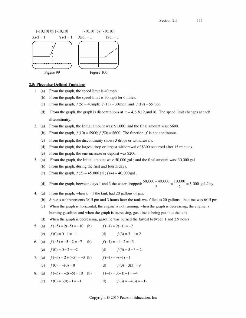
1. (a) From the graph, the speed limit is 40 mph.
(b) From the graph, the speed limit is 30 mph for 6 miles.
(c) From the graph, (5) 40mph;f (13) 30mph;f and (19) 55mph.f
(d) From the graph, the graph is discontinuous at 4,6,8,12,and16.x The speed limit changes at each
discontinuity.
2. (a) From the graph, the Initial amount was: $1,000; and the final amount was: $600.
(b) From the graph, (10) $900; (50) $600.f f The function f is not continuous.
(c) From the graph, the discontinuity shows 3 drops or withdrawals.
(d) From the graph, the largest drop or largest withdrawal of $300 occurred after 15 minutes.
(e) From the graph, the one increase or deposit was $200.
3. (a) From the graph, the Initial amount was: 50,000 gal.; and the final amount was: 30,000 gal.
(b) From the graph, during the first and fourth days.
(c) From the graph, (2) 45,000gal; (4) 40,000galf f .
(d) From the graph, between days 1 and 3 the water dropped:50,000 40,000 10,000
5,0002 2
gal./day.
4. (a) From the graph, when x = 1 the tank had 20 gallons of gas.
(b) Since x = 0 represents 3:15 pm and 3 hours later the tank was filled to 20 gallons, the time was 6:15 pm
(c) When the graph is horizontal, the engine is not running; when the graph is decreasing, the engine is
burning gasoline; and when the graph is increasing, gasoline is being put into the tank.
(d) When the graph is decreasing, gasoline was burned the fastest between 1 and 2.9 hours
5. (a) ( 5) 2( 5) 10f (b) ( 1) 2( 1) 2f
(c) (0) 0 1 1f (d) (3) 3 1 2f
6. (a) ( 5) 5 2 7f (b) ( 1) 1 2 3f
(c) (0) 0 2 2f (d) (3) 5 3 2f
7. (a) ( 5) 2 ( 5) 3f (b) ( 1) ( 1) 1f
(c) (0) (0) 0f (d) (3) 3(3) 9f
8. (a) ( 5) 2( 5) 10f (b) ( 1) 3( 1) 1 4f
(c) (0) 3(0) 1 1f (d) (3) 4(3) 12f

112 Chapter 2: Analysis of Graphs of Functions
Copyright © 2015 Pearson Education, Inc
9. Yes, continuous. See Figure 9.
10. Yes, continuous. See Figure 10.
11. Not continuous. See Figure 11
Figure 9 Figure 10 Figure 11
12. Not continuous. See Figure 12.
13. Not continuous. See Figure 13.
14. Not continuous. See Figure 14.
Figure 12 Figure 13 Figure 14
15. Not continuous. See Figure 15.
16. Not continuous. See Figure 16.
17. Yes, continuous. See Figure 17.
Figure 15 Figure 16 Figure 17
18. Not continuous. See Figure 18.
19. Yes, continuous. See Figure 19.
20. Yes, continuous. See Figure 20.
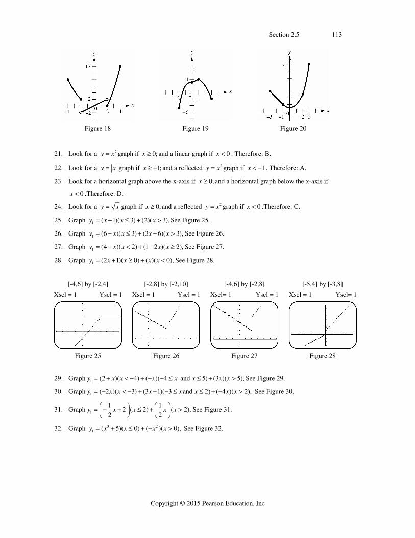
Section 2.5 113
Copyright © 2015 Pearson Education, Inc
Figure 18 Figure 19 Figure 20
21. Look for a 2y x graph if 0;x and a linear graph if 0x . Therefore: B.
22. Look for a y x graph if 1;x and a reflected 2y x graph if 1x . Therefore: A.
23. Look for a horizontal graph above the x-axis if 0;x and a horizontal graph below the x-axis if
0x .Therefore: D.
24. Look for a y x graph if 0;x and a reflected 2y x graph if 0x .Therefore: C.
25. Graph 1 ( 1)( 3) (2)( 3),y x x x See Figure 25.
26. Graph 1 (6 )( 3) (3 6)( 3),y x x x x See Figure 26.
27. Graph 1 (4 )( 2) (1 2 )( 2),y x x x x See Figure 27.
28. Graph 1 (2 1)( 0) ( )( 0),y x x x x See Figure 28.
[-4,6] by [-2,4] [-2,8] by [-2,10] [-4,6] by [-2,8] [-5,4] by [-3,8] Xscl = 1 Yscl = 1 Xscl = 1 Yscl = 1 Xscl= 1 Yscl = 1 Xscl = 1 Yscl= 1
Figure 25 Figure 26 Figure 27 Figure 28
29. Graph 1 (2 )( 4) ( )( 4 and 5) (3 )( 5),y x x x x x x x See Figure 29.
30. Graph 1 ( 2 )( 3) (3 1)( 3 and 2) ( 4 )( 2),y x x x x x x x See Figure 30.
31. Graph 1
1 12 ( 2) ( 2),
2 2y x x x x
⎛ ⎞ ⎛ ⎞ ⎜ ⎟ ⎜ ⎟⎝ ⎠ ⎝ ⎠
See Figure 31.
32. Graph 3 21 ( 5)( 0) ( )( 0),y x x x x See Figure 32.

114 Chapter 2: Analysis of Graphs of Functions
Copyright © 2015 Pearson Education, Inc
[-12,12] by [-6,20] [-6,6] by [-10,8] [-5,6] by [-2,4] [-3,4] by [-3,6] Xscl = 2 Yscl = 2 Xscl = 1 Yscl = 1 Xscl= 1 Yscl = 1 Xscl = 1 Yscl= 1
Figure 29 Figure 30 Figure 31 Figure 32
33. From the graph, the function is 2 if 0( ) ;domain : ,0 1, ; range: 1,2 .
1 if 1
xf x
x
⎧ ⎨ ⎩
34. From the graph, the function is 1 if 1( ) ;domain : , 1 2, ; range: 1,1 .
1 if 2
xf x
x
⎧ ⎨ ⎩
35. From the graph, the function is if 0( ) ;domain : , ; range: ,0 2 .
2 if 0
x xf x
x
⎧ ⎨ ⎩
36. From the graph, the function is 3 if 0
( ) ;domain : , ; range: 3 0, .if 0
xf x
x x
⎧⎪ ⎨⎪⎩
37. From the graph, the function is 3 if 1
( ) ;domain : , ; range : ,1 2, .1 if 1
x xf x
x x
⎧ ⎪ ⎨ ⎪⎩
38. From the graph, the function is 3 if 2( ) ;domain : , ; range : ,1 1, .
2 3 if 2
xf x
x x
⎧ ⎨ ⎩
39. There is an overlap of intervals since the number 4 satisfies both conditions. To be a function, every x-value
is used only once.
40. The value (4)f cannot be found since using the first formula, (4) 11,f and using the second
formula, (4) 16.f To have two different values violates the definition of function.
41. The graph of y x= is shifted 1.5 units downward.
42. The graph of y x= is reflected across the y-axis.
43. The graph of y x= is reflected across the x-axis.
44. The graph of y x= is shifted 2 units to the left.
45. Graph 1.5,y x= - See Figure 45.
46. Graph ,y x= - See Figure 46.
47. Graph ,y x=- See Figure 47.
48. Graph 2 ,y x= + See Figure 48.

Section 2.5 115
Copyright © 2015 Pearson Education, Inc
[-5,5] by [-3,3] [-5,5] by [-3,3] [-5,5] by [-3,3] [-5,5] by [-3,3] Xscl = 1 Yscl = 1 Xscl = 1 Yscl = 1 Xscl= 1 Yscl = 1 Xscl = 1 Yscl= 1
Figure 45 Figure 46 Figure 47 Figure 48
49. When 0 3x the slope is 5, which means the inlet pipe is open and the outlet pipe is closed; when
3 5x the slope is 2, which means both pipes are open; when 5 8x the slope is 0, which means both
pipes are closed; when 8 10x the slope is 3 , which means the inlet pipe is closed and the outlet pipe
is open.
50. (a) Since for each year given the shoe size is 1 size smaller than his age, the formula is 1y x
(b) From the table and question, graph the function. See figure 50.
51. (a) (1.5) 1.12, (3) 1.32,f f It costs $1.12 to mail 1.5 oz and $1.32 to mail 3 oz.
(b) Domain: 0,5 ; Range: 0.92,1.12,1.32,1.52,1.72 . See figure 51.
52. (a) (1967) 0.0475(1967) 93.3 0.1325f , In 1967, the average Super Bowl ad cost $0.1325 million.
(b) (1998) 0.475(1998) 93.3 1.605f , In 1998, the average Super Bowl ad cost $1.605 million.
(c) (2013) 0.1333(2013) 264.7284 3.6045f , In 2013, the average Super Bowl ad cost $3.6045
million.
(d) The function ( )f x is continuous on its domain since there are no breaks in the graph of ( )f x .
(e) See Figure 52.
Figure 50 Figure 51 Figure 52
53. (a) From the table, graph the piecewise function. See Figure 53.
(b) The likelihood of being a victim peaks from age 16 up to age 20, then decreases.
54. (a) From the table, graph the piecewise function. See Figure 54.
(b) Housing starts increased, decreased, and increased, with the maximum occurring during the 1960’s.
55. (a) From the graph, the highest speed is 55 mph and the lowest speed is 30 mph.
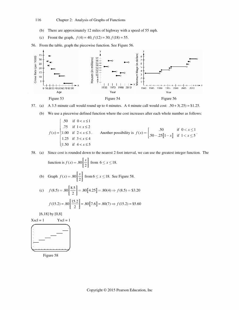
116 Chapter 2: Analysis of Graphs of Functions
Copyright © 2015 Pearson Education, Inc
(b) There are approximately 12 miles of highway with a speed of 55 mph.
(c) Fromt the graph, (4) 40; (12) 30; (18) 55.f f f
56. From the table, graph the piecewise function. See Figure 56.
Figure 53 Figure 54 Figure 56
57. (a) A 3.5 minute call would round up to 4 minutes. A 4 minute call would cost: .50 3(.25) $1.25.
(b) We use a piecewise defined function where the cost increases after each whole number as follows:
.50 if 0 1
.75 if 1 2
( ) 1.00 if 2 3
1.25 if 3 4
1.50 if 4 5
x
x
f x x
x
x
⎧⎪ ⎪⎪ ⎨⎪ ⎪
⎪⎩
. Another possibility is .50 if 0 1
( ).50 .25 1 if 1 5
xf x
x x
ì < £ïï=íï - - < £ïî.
58. (a) Since cost is rounded down to the nearest 2 foot interval, we can use the greatest integer function. The
function is ( ) .802
xf x =
from 6 18.x£ £
(b) Graph ( ) .802
xf x =
from 6 18.x£ £ See Figure 58.
(c) 8.5(8.5) .80 .80 4.25 .80(4) (8.5) $3.20
2f f= = = =
15.2(15.2) .80 .80 7.6 .80(7) (15.2) $5.60
2f f ⇒
[6,18] by [0,8] Xscl = 1 Yscl = 1
Figure 58

Section 2.6 117
Copyright © 2015 Pearson Education, Inc
59. For x in the interval 0, 2 , 25.y For x in the interval 2,3 , 25 3 28.y For x in the interval
3, 4 , 28 3 31y and so on. The graph is a step function. In this case, the first step has a different
width. See Figure 59.
60. Sketch a piecewise function that measures miles over minutes. The first piece increases at a rate of 40 mph
or 40 2
60 3 miles per minute, for 30 minutes (the time it takes to travel 20 miles at that rate). The second
piece stays at a constant distance of 20 miles for the 2 hour period at the park. The third piece decreases
(returns home) at a rate of 20 mph or 20 1
60 3 miles per minute, for 60 minutes (the time it takes to travel 20
miles at that rate). See Figure 60.
61. Sketch a piecewise function that fills a tank at a rate of 5 gallons a minute for the first 20 minutes (the time it
takes to fill the 100 gallon tank) and then drains the tank at a rate of 2 gallons per minute for 50 minutes (the
time it takes to drain the 100 gallon tank). See Figure 61.
Figure 59 Figure 60 Figure 61
62. (a) Use the points (1990, 1.3) and (2007, 2.7) to find the slope. 2.7 1.3 1.4
0.0822007 1990 17
m
1 1( ) 1.3 0.082( 1990) 0.082 161.88y y m x x y x y x ⇒ ⇒ Use the points (2007, 2.7) and
(2012, 1.75) to find the slope. 1.75 2.7 0.95
0.192012 2007 5
m
1 1( )y y m x x ⇒
1.75 0.19( 2012) 0.19 384.03y x y x ⇒ .
(b) Use the two functions above to create 0.082 161.88 1990 2007
( )0.19 384.03 2007 2012
x xf x
x x
⎧ ⎨ ⎩
2.6: Operations and Composition
1. 2 2(2 5) 2 5 .x x x x E ⇒
2. 2 2(2 5) 2 5 .x x x x B ⇒
3. 2 3 2(2 5) 2 5 .x x x x F ⇒
4. 2
.2 5
xD
x⇒
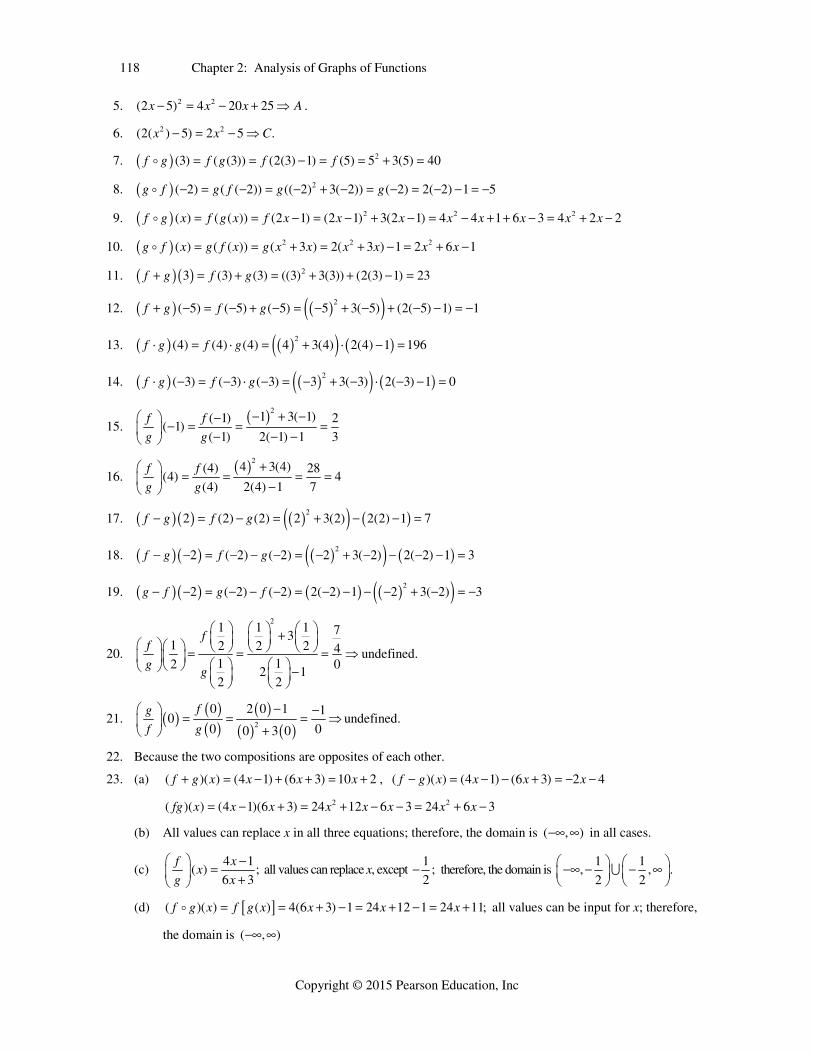
118 Chapter 2: Analysis of Graphs of Functions
Copyright © 2015 Pearson Education, Inc
5. 2 2(2 5) 4 20 25x x x A ⇒ .
6. 2 2(2( ) 5) 2 5 .x x C ⇒
7. 2(3) ( (3)) (2(3) 1) (5) 5 3(5) 40f g f g f f
8. 2( 2) ( ( 2)) (( 2) 3( 2)) ( 2) 2( 2) 1 5g f g f g g
9. 2 2 2( ) ( ( )) (2 1) (2 1) 3(2 1) 4 4 1 6 3 4 2 2f g x f g x f x x x x x x x x
10. 2 2 2( ) ( ( )) ( 3 ) 2( 3 ) 1 2 6 1g f x g f x g x x x x x x
11. 23 (3) (3) ((3) 3(3)) (2(3) 1) 23f g f g
12. 2( 5) ( 5) ( 5) 5 3( 5) (2( 5) 1) 1f g f g
13. 2(4) (4) (4) 4 3(4) 2(4) 1 196f g f g
14. 2( 3) ( 3) ( 3) 3 3( 3) 2( 3) 1 0f g f g
15. 2
1 3( 1)( 1) 2( 1)
( 1) 2( 1) 1 3
f f
g g
⎛ ⎞ ⎜ ⎟ ⎝ ⎠
16. 24 3(4)(4) 28
(4) 4(4) 2(4) 1 7
f f
g g
⎛ ⎞ ⎜ ⎟ ⎝ ⎠
17. 22 (2) (2) 2 3(2) 2(2) 1 7f g f g
18. 22 ( 2) ( 2) 2 3( 2) 2( 2) 1 3f g f g
19. 22 ( 2) ( 2) 2( 2) 1 2 3( 2) 3g f g f
20.
21 1 1 73
1 2 2 2 41 12 0
2 12 2
ff
gg
⎛ ⎞ ⎛ ⎞ ⎛ ⎞⎜ ⎟ ⎜ ⎟ ⎜ ⎟⎛ ⎞⎛ ⎞ ⎝ ⎠ ⎝ ⎠ ⎝ ⎠ ⇒⎜ ⎟⎜ ⎟ ⎛ ⎞ ⎛ ⎞⎝ ⎠⎝ ⎠ ⎜ ⎟ ⎜ ⎟⎝ ⎠ ⎝ ⎠
undefined.
21.
2
0 2 0 1 10
0 00 3 0
fg
f g
⎛ ⎞ ⇒⎜ ⎟⎝ ⎠
undefined.
22. Because the two compositions are opposites of each other.
23. (a) ( )( ) (4 1) (6 3) 10 2f g x x x x , ( )( ) (4 1) (6 3) 2 4f g x x x x
2 2( )( ) (4 1)(6 3) 24 12 6 3 24 6 3fg x x x x x x x x
(b) All values can replace x in all three equations; therefore, the domain is ( , ) in all cases.
(c) 4 1
( ) ;6 3
f xx
g x
⎛ ⎞ ⎜ ⎟ ⎝ ⎠ all values can replace x, except
1;
2 therefore, the domain is
1 1, , .
2 2⎛ ⎞ ⎛ ⎞ ⎜ ⎟ ⎜ ⎟⎝ ⎠ ⎝ ⎠
(d) ( )( ) ( ) 4(6 3) 1 24 12 1 24 11;f g x f g x x x x all values can be input for x; therefore,
the domain is ( , )

Section 2.6 119
Copyright © 2015 Pearson Education, Inc
(e) ( )( ) ( ) 6(4 1) 3 24 6 3 24 3;g f x g f x x x x all values can replace x; therefore, the
domain is ( , ) .
24. (a) ( )( ) (9 2 ) ( 5 2) 7 11f g x x x x , ( )( ) (9 2 ) ( 5 2) 3 7f g x x x x
2 2( )( ) (9 2 )( 5 2) 45 18 10 4 10 49 18fg x x x x x x x x
(b) All values can replace x in all three equations; therefore, the domain is ( , ) in all cases.
(c) 9 2
( ) ;5 2
f xx
g x
⎛ ⎞ ⎜ ⎟ ⎝ ⎠all values can replace x, except
2
5; therefore, the domain is
2 2, , .5 5
⎛ ⎞ ⎛ ⎞ ⎜ ⎟ ⎜ ⎟⎝ ⎠ ⎝ ⎠
(d) ( )( ) ( ) 9 2( 5 2) 9 10 4 10 5;f g x f g x x x x all values can replace x; therefore, the
domain is ( , )
(e) ( )( ) ( ) 5(9 2 ) 2 45 10 2 10 43;g f x g f x x x x all values can replace x; therefore,
the domain is ( , )
25. (a) ( )( ) 3 2f g x x x , ( )( ) 3 2f g x x x , ( )( ) 3 (2 )fg x x x
(b) All values can replace x in all three equations; therefore, the domain is ( , ) in all cases.
(c) 3
( ) ;2
xfx
g x
⎛ ⎞⎜ ⎟
⎝ ⎠ all values can replace x, except 0; therefore, the domain is ( ,0) (0, )
(d) ( )( ) ( ) (2 ) 3 2 3 ;f g x f g x x x all values can replace x; therefore, the domain is ( , ).
(e) ( )( ) ( ) 2 3 2 3 ;g f x g f x x x all values can replace x; therefore, the domain is ( , )
26. (a) ( )( ) 2 4 ( 1) 2 4 1f g x x x x x , ( )( ) 2 4 ( 1) 2 4 1f g x x x x x
( )( ) 2 4 ( 1) ( 1) 2 4fg x x x x x
(b) All values can replace x in all three equations; therefore, the domain is ( , ) in all cases.
(c) 2 4
( )1
xfx
g x
⎛ ⎞⎜ ⎟ ⎝ ⎠
all values can replace x, except 1; therefore, the domain is ( , 1) ( 1, ).
(d) ( )( ) ( ) 2( 1) 4 2 2 ;f g x f g x x x all values can replace x, so the domain is ( , ).
(e) ( )( ) ( ) 2 4 1;g f x g f x x all values can replace x, so the domain is ( , ).
27. (a) 3 33 3( )( ) 4 ( 5) 4 5f g x x x x x , 3 33 3( )( ) 4 ( 5) 4 5f g x x x x x
33( )( ) 4 ( 5)fg x x x
(b) All values can replace x in all three equations; therefore, the domain is ( , ) in all cases.
(c) 3
3
4( )
( 5)
f xx
g x
⎛ ⎞ ⎜ ⎟ ⎝ ⎠ all values can replace x, except 3 5 , so the domain is 3 3( , 5) ( 5, ).
(d) 33 33( )( ) ( ) ( 5) 4 9 ;f g x f g x x x all values can replace x, so the domain is ( , ).

120 Chapter 2: Analysis of Graphs of Functions
Copyright © 2015 Pearson Education, Inc
(e) 33( )( ) ( ) 4 5 4 5 9;g f x g f x x x x all values can replace x, so the domain is
( , ).
28. (a) 3 33 3( )( ) 6 3 (2 1) 6 3 2 1f g x x x x x
3 33 3( )( ) 6 3 (2 1) 6 3 2 1f g x x x x x
33( )( ) 6 3 (2 1)fg x x x
(b) All values can replace x in all three equations; therefore, the domain is ( , ) in all cases.
(c) 3
3
6 3( ) ;
(2 1)
f xx
g x
⎛ ⎞ ⎜ ⎟ ⎝ ⎠ all values can replace x, except 3
1
2 , so the domain
is 3 31 1
, ,2 2
⎛ ⎞ ⎛ ⎞ ⎜ ⎟ ⎜ ⎟⎜ ⎟ ⎜ ⎟⎝ ⎠ ⎝ ⎠
(d) 33 33( )( ) ( ) 6 3(2 1) 6 3;f g x f g x x x all values can replace x, so the domain is
( , ).
(e) 33( )( ) ( ) 2 6 3 1 2(6 3 ) 1 6 13;g f x g f x x x x all values can replace x; therefore,
the domain is ( , ).
29. (a) 2 2( )( ) 3 ( 1) 3 1f g x x x x x , 2 2( )( ) 3 ( 1) 3 1f g x x x x x
2( )( ) 3 ( 1)fg x x x
(b) All values can replace x in all three equations; therefore, the domain is ( , ) in all cases.
(c) 2 3
( ) ;( 1)
f xx
g x
⎛ ⎞ ⎜ ⎟ ⎝ ⎠ all values can replace x, except 1; therefore, the domain is , 1 1, .
(d) 2 2 2( )( ) ( ) ( 1) 3 2 1 3 2 4;f g x f g x x x x x x all values can replace x;
therefore, the domain is ( , ).
(e) 2 2( )( ) ( ) 3 1 3 1;g f x g f x x x all values can replace x; therefore, the domain is,
( , ).
30. (a) 2 2( )( ) 2 4 ( ) 2 4f g x x x x x , 2 2( )( ) 2 4 ( ) 2 4f g x x x x x
2 2( )( ) 2 4 ( ) 2 4fg x x x x x
(b) All values can replace x in all three equations; therefore, the domain is ( , ) in all cases.
(c) 22 4
( ) ;f x
xg x
⎛ ⎞ ⎜ ⎟⎝ ⎠
all values can replace x, except 0; therefore, the domain is ,0 0, .

Section 2.6 121
Copyright © 2015 Pearson Education, Inc
(d) 2 2( )( ) ( ) 2 4( ) 2 4 ;f g x f g x x x all values can replace x; therefore, the domain is
( , ).
(e) 2 2( )( ) ( ) 2 4 2 4 ;g f x g f x x x all values can replace x; therefore, the domain
is ( , ).
31. (a) From the graph, 4 ( 2) 2.
(b) From the graph, 1 ( 3) 4.
(c) From the graph, (0)( 4) 0.
(d) From the graph, 1 1
.3 3
32. (a) From the graph, 0 2 2.
(b) From the graph, 2 1 3.
(c) From the graph, (2)(1) 2.
(d) From the graph, 4
2.2
33. (a) From the graph, 0 3 3.
(b) From the graph, 1 4 5.
(c) From the graph, (2)(1) 2.
(d) From the graph, 3
0⇒ undefined.
34. (a) From the graph, 3 1 2.
(b) From the graph, 2 0 2.
(c) From the graph, ( 3)( 1) 3.
(d) From the graph, 3
3.1
35. (a) From the table, 7 ( 2) 5.
(b) From the table, 10 5 5.
(c) From the table, (0)(6) 0.
(d) From the table, 5
0 undefined.
36. (a) From the table, 5 4 9.
(b) From the table, 0 0 0.
(c) From the table, ( 4)(2) 8.
(d) From the table, 8
8.1
37. See Table 37.
38. See Table 38.

122 Chapter 2: Analysis of Graphs of Functions
Copyright © 2015 Pearson Education, Inc
Figure 37 Figure 38
39. (2004) 260 and (2004) 400 (2004) (2004) (2004) 260 400 660M F T M F
40. (2008) 290 and (2008) 470 (2008) (2008) (2008) 290 470 760M F T M F
41. The slopes of the line segments for the period 2000-2004 are much steeper than the slopes of the
corresponding line segments for the period 2004-2008. Thus, the number of associate’s degrees increased
more rapidly during the period 2000-2004.
42. If 2000 2008, ( ) , and ( ) , then ( )k T k r F k s M k r s .
43. 2000 (2000) (2000) 19 13 6T S T S , This represents the billions of dollars spent for general
science in 2000.
44. 2010 (2010) (2010) 29 11 18T G T G , This represents the billions of dollars spent for space
and other technologies in 2010.
45. In space and other technologies spending was almost static in the years 1995-2000.
46. In space and other technologies spending increased the most during the years 2005-2010.
47. (a) ( )(4) (4) ,f g f g so from the graph find (4) 0.g Now find (0) 4;f therefore, ( )(4) 4.f g
(b) ( )(3) (3) ,g f g f so from the graph find (3) 2.f Now find 2 2;g therefore, ( )(3) 2.g f
(c) ( )(2) (2) ,f f f f so from the graph find (2) 0.f Now find (0) 4;f therefore, ( )(2) 4.f f
48. (a) ( )(2) (2) ,f g f g so from the graph find (2) 2.g Now find ( 2) 4;f therefore,
( )(2) 4.f g
(b) ( )(0) (0) ,g g g g so from the graph find (0) 2.g Now find (2) 2;g therefore, ( )(0) 2.g g
(c) ( )(4) (4) ,g f g f so from the graph find (4) 2.f Now find (2) 2;g therefore,
( )(4) 2.g f
49. (a) ( )(1) (1) ,f g f g so from the graph find (1) 2.g Now find (2) 3;f therefore, ( )(1) 3.f g
(b) ( )( 2) ( 2) ,g f g f so from the graph find ( 2) 3.f Now find ( 3) 2;g therefore,
( )( 2) 2.g f
(c) ( )( 2) ( 2) ,g g g g so from the graph find ( 2) 1.g Now find ( 1) 0;g therefore,
( )( 1) 0.g g
50. (a) ( )( 2) ( 2) ,f g f g so from the graph find ( 2) 4.g Now find (4) 2;f therefore,
( )( 2) 2.f g
(b) ( )(1) (1) ,g f g f so from the graph find (1) 1.f Now find (1) 1;g therefore, ( )(1) 1.g f

Section 2.6 123
Copyright © 2015 Pearson Education, Inc
(c) ( )(0) (0) ,f f f f so from the graph find (0) 0.f Now find (0) 0;f therefore, ( )(0) 0.f f
51. (a) ( )(1) (1) ,g f g f so from the table find (1) 4.f Now find (4) 5;g therefore, ( )(1) 5.g f
(b) ( )(4) (4) ,f g f g so from the table find (4) 5.g (5)f is undefined; therefore, ( )(4)f g is
undefined.
(c) ( )(3) (3) ,f f f f so from the table find (3) 1.f Now find (1) 4;f therefore, ( )(3) 4.f f
52. (a) ( )(1) (1) ,g f g f so from the table find (1) 2.f Now find (2) 4;g therefore, ( )(1) 4g f .
(b) ( )(4) (4) ,f g f g so from the table we find 4g is undefined; therefore, ( )(4)f g is undefined.
(c) ( )(3) (3) ,f f f f so from the table find (3) 6.f Now find (6) 7;f therefore, ( )(3) 7.f f
53. From the table, (3) 4g and (4) 2.f
54. From the table, (6) 7f and (7) 0.g
55. Since 3 1 2Y Y Y and 1,X we solve 1 2 ( 1) .Y Y First solve 22 ( 1) 1,Y now solve 1 2 1 5 3;Y
therefore, 3 3.Y
56. Since 3 1 2Y Y Y and 2,X we solve 1 2 ( 2) .Y Y First solve 22 ( 2) 4,Y now solve 1 2(4) 5 3;Y
therefore, 3 3.Y
57. Since 3 1 2Y Y Y and 7,X we solve 1 2 (7) .Y Y First solve 2
2 7 49,Y now solve 1 2(49) 5 93;Y
therefore, 3 93.Y
58. Since 3 1 2Y Y Y and 8,X we solve 1 2 (8) .Y Y First solve 2
2 8 64,Y now solve
1 2(64) 5 123;Y therefore, 3 123.Y
59. (a) 2 3( )( ) ( ) ( 3 1) ;f g x f g x x x all values can be input for x; therefore, the domain is ( , ).
(b) 3 2 3 6 3( )( ) ( ) ( ) 3( ) 1 3 1;g f x g f x x x x x all values can be input for x; therefore, the
domain is ( , ).
(c) 3 3 9( )( ) ( ) ( ) ;f f x f f x x x all values can be input for x; therefore, the domain is ( , ).
60. (a) 2 2
1 1( )( ) ( ) 2 2 ;f g x f g x
x x⎛ ⎞ ⎜ ⎟⎝ ⎠
all values can be input for x, except 0; therefore, the domain
is ( ,0) (0, ).
(b) 2
1( )( ) ( ) ;
(2 )g f x g f x
x
all values can be input for x, except 2; therefore, the domain is
( , 2) (2, ).
(c) ( )( ) ( ) 2 (2 ) ;f f x f f x x x all values can be input for x; therefore, the domain is ( , ).
61. (a) 2
( )( ) ( ) 1 1 ;f g x f g x x x all values can be input for x; therefore, the domain is ( , ).

124 Chapter 2: Analysis of Graphs of Functions
Copyright © 2015 Pearson Education, Inc
(b) 2 2( )( ) ( ) 1 ( ) 1 ;g f x g f x x x only values where 2 1x can be input for x; therefore,
the domain is 1,1 .
(c) 2 2 4( )( ) ( ) ( ) ;f f x f f x x x all values can be input for x; therefore, the domain is ( , ).
62. (a) 4 2 4 2( )( ) ( ) ( 3 4) 2 3 2;f g x f g x x x x x x x all values can be input for x; therefore,
the domain is ( , ).
(b) 4 2( )( ) ( ) ( 2) ( 2) 3( 2) 4;g f x g f x x x x all values can be input for x; therefore, the
domain is ( , ).
(c) ( )( ) ( ) ( 2) 2 4;f f x f f x x x all values can be input for x; therefore, the domain is ( , ).
63. (a) 1 1
( )( ) [ ( )] ;(5 ) 1 5 1
f g x f g xx x
all values can be input for x, except 1
;5
therefore, the domain
is 1 1
, , .5 5
⎛ ⎞ ⎛ ⎞ ⎜ ⎟ ⎜ ⎟⎝ ⎠ ⎝ ⎠
(b) 1 5
( )( ) [ ( )] 5 ;1 1
g f x g f xx x
⎛ ⎞ ⎜ ⎟ ⎝ ⎠ all values can be input for x, except, −1; therefore, the domain
is ( . 1) ( 1, ).
(c) 1 1 1 1
( )( ) [ ( )] ;1 1 21 2
11 1 11
xf f x f f x
x x xx x xx
⎛ ⎞ ⎜ ⎟ ⎝ ⎠
all values can be input for x, except
those that make 1
02
x
x
or undefined. That would be −1 and −2; therefore, the domain is
( , 2) ( 2, 1) ( 1, ).
64. (a) 2 2( )( ) [ ( )] ( 4 ) 4 4 4;f g x f g x x x only values where 2 4x can be input for x;
therefore, the domain is [−2, 2].
(b) 2( )( ) [ ( )] 4 ( 4) ;g f x g f x x only values where 2( 4) 4x can be input for x; therefore, the
domain is [−6, −2].
(c) ( )( ) [ ( )] ( 4) 4 8;f f x f f x x x all values can be input for x; therefore, the domain is ( , ).
65. (a) 3 2 3 2( )( ) [ ( )] 2(4 5 ) 1 8 10 1;f g x f g x x x x x all values can be input for x; therefore, the domain
is ( , ).
(b) 3 2( )( ) [ ( )] 4(2 1) 5(2 1)g f x g f x x x 3 2 24(8 12 6 1) 5(4 4 1)x x x x x
3 2 2 3 232 48 24 4 (20 20 5) 32 28 4 1;x x x x x x x x all values can be input for x; therefore, the
domain is ( , ).
(c) ( )( ) [ ( )] 2(2 1) 1 4 3;f f x f f x x x all values can be input for x; therefore, the domain is
( , ).

Section 2.6 125
Copyright © 2015 Pearson Education, Inc
66. (a) (2 3) 3 2
( )( ) [ ( )] ;2 3
x xf g x f g x x
all values can be input for x; therefore, the domain is
( , ).
(b) 3
( )( ) [ ( )] 2 3 ( 3) 3 ;2
xg f x g f x x x
⎛ ⎞ ⎜ ⎟⎝ ⎠
all values can be input for x; therefore, the domain
is ( , ).
(c)
3 3 6 93
92 2 2 2( )( ) [ ( )] ;
2 2 2 4
x x xx
f f x f f x
⎛ ⎞ ⎛ ⎞ ⎛ ⎞ ⎜ ⎟ ⎜ ⎟ ⎜ ⎟ ⎝ ⎠ ⎝ ⎠ ⎝ ⎠ all values can be input for x;
therefore, the domain is ( , ).
67. (a) ( ) ( ( )) (5) 5,f g x f g x f all values can be input for x, thefore the domain is , .
(b) ( ) ( ( )) (5) 5,g f x g f x g all values can be input for x, therefore the domain is , .
(c) ( ) ( ( )) (5) 5,f f x f f x f all values can be input for x, therefore the domain is , .
68. Let ( )f x c , then ( ) ( ) ( ) .f f x f f x f c c Therefore, there is only one value in the range of
( )f f x .
69. 1
( )( ) [ ( )] 4 ( 2) 2 2 24
f g x f g x x x x⎛ ⎞ ⎜ ⎟⎝ ⎠
, 1 1
( )( ) [ ( )] ((4 2) 2) (4 )4 4
g f x g f x x x x
70. 1
( )( ) [ ( )] 33
f g x f g x xx
⎛ ⎞ ⎜ ⎟⎝ ⎠
, 1
( )( ) [ ( )] ( 3 )3
g f x g f x x x
71. 33 3 3331 4
( ) 5 4 4 45 5
f g x f g x x x x x⎛ ⎞ ⎡ ⎤ ⎜ ⎟⎣ ⎦ ⎝ ⎠
3
31 4 1 4 4 4( ) 5 4 5 4
5 5 5 5 5 5g f x g f x x x x x ⎡ ⎤⎣ ⎦
72. 33 33( ) 1 1f g x f g x x x x ⎡ ⎤⎣ ⎦ , 33( ) 1 1 1 1g f x g f x x x x ⎡ ⎤⎣ ⎦
73. Graph 331 26, 6,y x y x and 3y x in the same viewing window. See Figures 73. The graph of 2y
can be obtained by reflecting the graph of 1y across the line 3 .y x
74. Graph 1 2
15 3, 3 ,
5y x y x and 3y x in the same viewing window. See Figures 74. The graph of 2y
can be obtained by reflecting the graph of 1y across the line 3 .y x
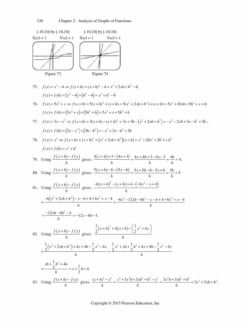
126 Chapter 2: Analysis of Graphs of Functions
Copyright © 2015 Pearson Education, Inc
[-10,10] by [-10,10] [-10,10] by [-10,10] Xscl = 1 Yscl = 1 Xscl = 1 Yscl = 1
Figure 73 Figure 74
75. 2 2 2 2( ) 4 ( ) ( ) 4 2 4;f x x f x h x h x xh h
2 2 2 2( ) ( ) 4 4 8f x f h x h x h
76. 2 2 2 2 2 2( ) 5 ( ) 5( ) ( ) 5( 2 ) ( ) 5 10 5 ;f x x x f x h x h x h x xh h x h x xh h x h
2 2 2 2( ) ( ) 5 5 5 5f x f h x x h h x x h h
77. 2 2 2 2 2 2( ) 3 ( ) 3( ) ( ) 3 3 2 2 3 3f x x x f x h x h x h x h x xh h x xh x h h ;
2 2 2 2( ) ( ) 3 3 3 3f x f h x x h h x x h h
78. 3 3 2 2 3 2 2 3( ) ( ) ( ) 2 3 3f x x f x h x h x xh h x h x hx h x h
3 3( ) ( )f x f h x h
79. Using f x h f x
h
gives:
4 3 4 3 4 4 3 4 3 44.
x h x x h x h
h h h
80. Using f x h f x
h
gives:
5 6 5 6 5 5 6 5 6 55.
x h x x h x h
h h h
81. Using f x h f x
h
gives:
2 26 4 6 4x h x h x x
h
= 2 2 26 2 4 6 4x xh h x h x x
h
=
2 2 26 12 6 4 6 4x xh h x h x x
h
212 6
12 6 1.xh h h
x hh
82. Using f x h f x
h
gives:
2 21 14 4
2 2x h x h x x
h
⎛ ⎞ ⎜ ⎟⎝ ⎠
= 2 2 2 2 2 21 1 1 1 1
2 4 4 4 4 4 42 2 2 2 2
x xh h x h x x x xh h x h x x
h h
=
214 12 4.
2
xh h hx h
h
83. Using ( ) ( )f x h f x
h
gives:
3 3 3 2 2 3 3 2 2 32 2( ) 3 3 3 3
3 3 .x h x x x h xh h x x h xh h
x xh hh h h

Section 2.6 127
Copyright © 2015 Pearson Education, Inc
84. Using ( ) ( )f x h f x
h
gives:
3 3 3 2 2 3 32( ) ( 2 ) 2( 3 3 ) 2x h x x x h xh h x
h h
3 2 2 3 3 2 2 32 6 6 2 2 6 6 2x x h xh h x x h xh h
h h
2 26 6 2 .x xh h
85. Using ( ) ( )f x h f x
h
gives:
2 2 22 2 1 2 11 ( ) (1 ) x xh h xx h x
h h
2 2 2 21 2 1 2
2x xh h x xh h
x hh h
86. Using ( ) ( )f x h f x
h
gives:
2 2 22 2 2 2 2 2( ) 2( ) ( 2 ) x xh h x h x xx h x h x x
h h
22 2
2 2xh h h
x hh
87. Using ( ) ( )f x h f x
h
gives:
2 2 22 2 3 2 33( ) (3 ) x xh h xx h x
h h
2 2 2 23 6 3 3 6 3
6 3x xh h x xh h
x hh h
88. Using ( ) ( )f x h f x
h
gives:
x h x x h xx h x x h x
h h x h x h x h x
1h
x h xh x h x
89. Using ( ) ( )f x h f x
h
gives:
2 (2 2 ) 21 12 2 2 2 2 2 12( ) 2
2 ( )
x x h h
x x h x x hx h x
h h h x x h
90. Using ( ) ( )f x h f x
h
gives:
2 2 2 2 2 2
2 2 22 2 22 2
( ) 2 21 1( )
x x h x x xh h xh h
x x h x x h x x hx h x
h h h h
22
22
( 2 )
2
h x h
x x h x h
h x x h
91. One possible solution is 2( )f x x and ( ) 6 2.g x x Then 2( )( ) [ ( )] (6 2) .f g x f g x x
92. One possible solution is 2( )f x x and 2( ) 11 12 .g x x x Then 2 2( )( ) [ ( )] (11 12 ) .f g x f g x x x
93. One possible solution is ( )f x x and 2( ) 1.g x x Then 2( )( ) [ ( )] 1.f g x f g x x
94. One possible solution is 3( )f x x and ( ) 2 3.g x x Then 3( )( ) [ ( )] (2 3) .f g x f g x x
95. One possible solution is ( ) 12f x x and ( ) 6 .g x x Then ( )( ) [ ( )] 6 12.f g x f g x x
96. One possible solution is 3( ) 4f x x and ( ) 2 3.g x x Then 3( )( ) [ ( )] 2 3 4.f g x f g x x
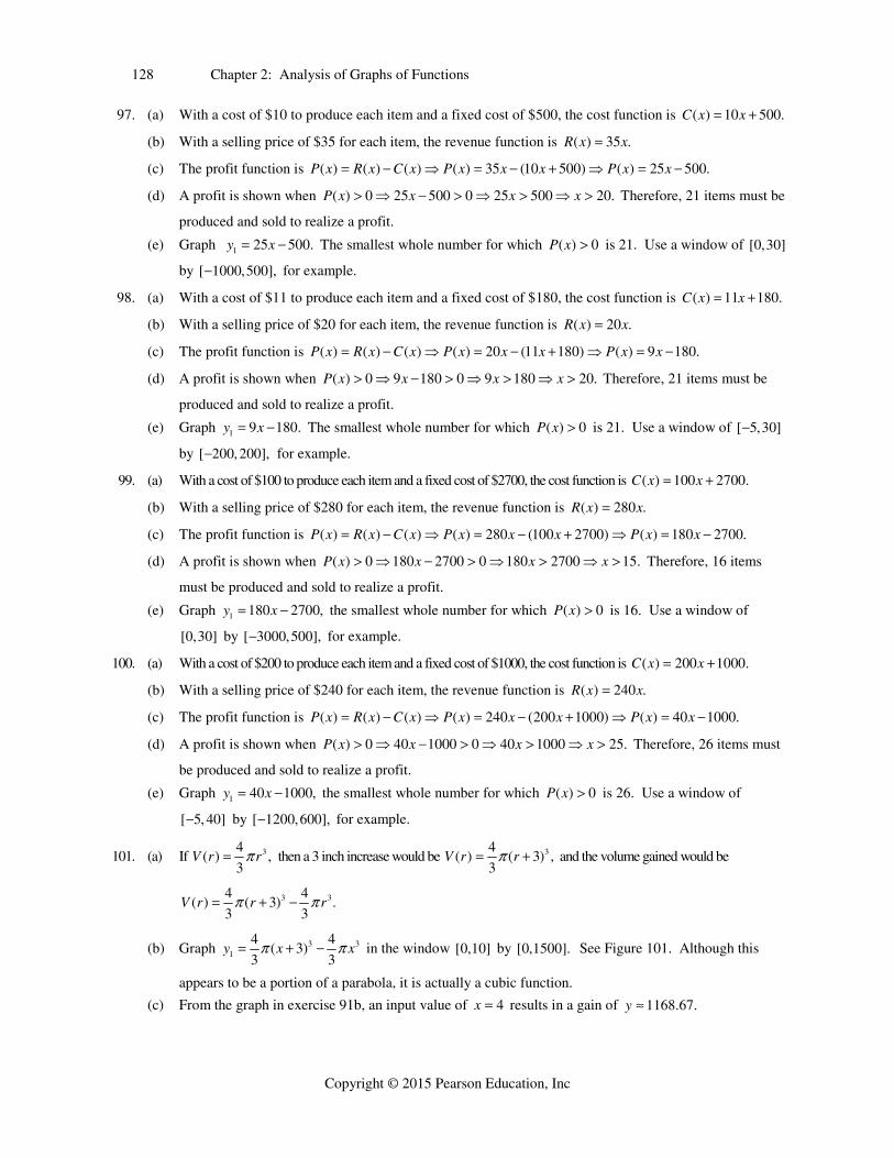
128 Chapter 2: Analysis of Graphs of Functions
Copyright © 2015 Pearson Education, Inc
97. (a) With a cost of $10 to produce each item and a fixed cost of $500, the cost function is ( ) 10 500.C x x
(b) With a selling price of $35 for each item, the revenue function is ( ) 35 .R x x
(c) The profit function is ( ) ( ) ( ) ( ) 35 (10 500) ( ) 25 500.P x R x C x P x x x P x x ⇒ ⇒
(d) A profit is shown when ( ) 0 25 500 0 25 500 20.P x x x x ⇒ ⇒ ⇒ Therefore, 21 items must be
produced and sold to realize a profit.
(e) Graph 1 25 500.y x The smallest whole number for which ( ) 0P x is 21. Use a window of [0,30]
by [ 1000,500], for example.
98. (a) With a cost of $11 to produce each item and a fixed cost of $180, the cost function is ( ) 11 180.C x x
(b) With a selling price of $20 for each item, the revenue function is ( ) 20 .R x x
(c) The profit function is ( ) ( ) ( ) ( ) 20 (11 180) ( ) 9 180.P x R x C x P x x x P x x ⇒ ⇒
(d) A profit is shown when ( ) 0 9 180 0 9 180 20.P x x x x ⇒ ⇒ ⇒ Therefore, 21 items must be
produced and sold to realize a profit.
(e) Graph 1 9 180.y x The smallest whole number for which ( ) 0P x is 21. Use a window of [ 5,30]
by [ 200,200], for example.
99. (a) With a cost of $100 to produce each item and a fixed cost of $2700, the cost function is ( ) 100 2700.C x x
(b) With a selling price of $280 for each item, the revenue function is ( ) 280 .R x x
(c) The profit function is ( ) ( ) ( ) ( ) 280 (100 2700) ( ) 180 2700.P x R x C x P x x x P x x ⇒ ⇒
(d) A profit is shown when ( ) 0 180 2700 0 180 2700 15.P x x x x ⇒ ⇒ ⇒ Therefore, 16 items
must be produced and sold to realize a profit.
(e) Graph 1 180 2700,y x the smallest whole number for which ( ) 0P x is 16. Use a window of
[0,30] by [ 3000,500], for example.
100. (a) With a cost of $200 to produce each item and a fixed cost of $1000, the cost function is ( ) 200 1000.C x x
(b) With a selling price of $240 for each item, the revenue function is ( ) 240 .R x x
(c) The profit function is ( ) ( ) ( ) ( ) 240 (200 1000) ( ) 40 1000.P x R x C x P x x x P x x ⇒ ⇒
(d) A profit is shown when ( ) 0 40 1000 0 40 1000 25.P x x x x ⇒ ⇒ ⇒ Therefore, 26 items must
be produced and sold to realize a profit.
(e) Graph 1 40 1000,y x the smallest whole number for which ( ) 0P x is 26. Use a window of
[ 5, 40] by [ 1200,600], for example.
101. (a) If 34( ) ,
3V r r then a 3 inch increase would be 34
( ) ( 3) ,3
V r r and the volume gained would be
3 34 4( ) ( 3) .
3 3V r r r
(b) Graph 3 31
4 4( 3)
3 3y x x in the window [0,10] by [0,1500]. See Figure 101. Although this
appears to be a portion of a parabola, it is actually a cubic function.
(c) From the graph in exercise 91b, an input value of 4x results in a gain of 1168.67.y
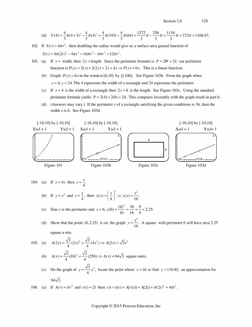
Section 2.6 129
Copyright © 2015 Pearson Education, Inc
(d) 3 34 4 4 4 1372 256 1116(4) (4 3) (4) (343) (64) 372 1168.67.
3 3 3 3 3 3 3V
102. If 2( ) 4 ,S r r then doubling the radius would give us a surface area gained function of
2 2 2 2 2( ) 4 (2 ) 4 16 4 12 .S r r r r r r
103. (a) If x width, then 2x length. Since the perimeter formula is 2 2P W L our perimeter
function is ( ) 2( ) 2(2 ) 2 4 ( ) 6 .P x x x x x P x x ⇒ This is a linear function.
(b) Graph ( ) 6P x x in the window[0,10] by [1,100]. See Figure 103b. From the graph when
4, 24.x y The 4 represents the width of a rectangle and 24 represents the perimeter.
(c) If 4x is the width of a rectangle then 2 8x is the length. See Figure 103c. Using the standard
perimeter formula yields 2(4) 2(8) 24.P This compares favorably with the graph result in part b.
(d) (Answers may vary.) If the perimeter y of a rectangle satisfying the given conditions is 36, then the
width x is 6. See Figure 103d.
[-10,10] by [-10,10] [-10,10] by [-10,10] [-10,10] by [-10,10] Xscl = 1 Yscl = 1 Xscl = 1 Yscl = 1 Xscl = 1 Yscl= 1
Figure 101 Figure 103b Figure 103c Figure 103d
104. (a) If 4x s then .4
xs
(b) If 2y s and ,4
xs then
2 2
( ) ( ) .4 16
x xy x y x
⎛ ⎞ ⇒ ⎜ ⎟⎝ ⎠
(c) Sine x is the perimeter and 2(6) 36 9
6, (6) 2.25.16 16 4
x y
(d) Show that the point (6,2.25) is on the graph 2
.16
xy A square with perimeter 6 will have area 2.25
square u nits.
105. (a) 2 2 23 3(2 ) (2 ) (4 ) (2 ) 3
4 4A x x x A x x ⇒
(b) 23 3( ) (16) (256) ( ) 64 3
4 4A x A x ⇒ square units.
(c) On the graph of 23,
4y x locate the point where 16x to find 110.85,y an approximation for
64 3.
106. (a) If 2( )A r r and ( ) 2r t t then 2 2( )( ) [ ( )] [2 ] (2 ) 4 .A r t A r t A t t t

130 Chapter 2: Analysis of Graphs of Functions
Copyright © 2015 Pearson Education, Inc
(b) ( )( )A r t is a composite function that expresses the area of the circular region covered by the pollutants
as a function of time t (in hours).
(c) Since 0t is 8 A.M., noon would be 2 24. ( )(4) 4 (4) 64 mi .t A r
(d) Graph 21 4y x and show that for 4, 201x y (an approximation for 64 ).
107. (a) (2100) 42,A ; The average age of a person in 2100 is projected to be 42 years. (2100) 430T , In
2100, the living world’s population will have a combined life experience of 430 billion years.
(b) (2100) 430
10.2(2100) 42
T
A , The world population will be about 10.2 billion in 2100.
(c) P(x) gives the world’s population during year x.
108. (a) The domain is the years. See table below. Therefore, D= { 2009, 2010, 2011, 2012 }.
x 2009 2010 2011 2012
h(x) 77.5 78.1 75.3 76.1
(b) The function h computes the number of acres of soybeans harvested in the U.S. in millions of acres.
109. (a) ( )(2010) 13.0 74.3 87.3f g
(b) The function ( )( )f g x computes the total 2SO and Carbon Monoxide during year x.
(c) Add functions f and g.
x 1970 1980 1990 2000 2010
(f+g)(x) 235.2 211.3 177.3 130.8 87.3
110. (a) The function h is the addition of functions f and g.
x 1990 2000 2010 2020 2030
h(x) 32 35.5 39 42.5 46
(b) The function h is the addition of functions f and g. Therefore, ( ) ( ) ( ).h x f x g x
111. (a) The function h is the subtraction of function f from g. Therefore, ( ) ( ) ( ).h x g x f x
(b) (1996) (1996) (1996) 841 694 147h g f , (2006) (2006) (2006) 1165 1012 153h g f
(c) Using the points (1996, 147) and (2006, 153) from part b, the slope is 153 147 6
.6.2006 1996 10
m
Now
using point slope form: 147 .6( 1996) .6( 1996) 147.y x y x ⇒
112. (a) Graph 2
2
1900( 1982) 619( ) ,
3200( 1982) 1586
xh x
x
in the window [1982, 1994] by [0, 1] See Figure 112a.
Approximately 59% of the people who contracted AIDS during this time period died.
(b) Divide number of deaths by number of cases for each year. The results compare favorably with the
graph. See Figure 112b.

Section 2.6 131
Copyright © 2015 Pearson Education, Inc
[-10,10] by [-10,10] Xscl = 1 Yscl = 1
Figure 112a Figure 112b
Reviewing Basic Concepts (Sections 2.4—2.6)
1. (a) 1 1 1
2 4 2 4 2 42 2 2
x x x x ⇒ ⇒ ⇒ or 1 1
2 4 6 12.2 2
x x x ⇒ ⇒
Therefore, the solution set is 12,4 .
(b) 1 1 1
2 4 2 4 2 42 2 2
x x x x ⇒ ⇒ ⇒ or 1 1
2 4 6 12.2 2
x x x ⇒ ⇒ Therefore, the
solution interval is ( , 12) (4, ).
(c) 1 1 1
2 4 4 2 4 6 2 12 4.2 2 2
x x x x ⇒ ⇒ ⇒
Therefore, the solution interval is [-12,4].
2. For the graph of | ( ) |,y f x we reflect the graph of ( )y f x across the x-axis for all points for which
0.y Where 0,y the graph remains unchanged. See Figure 2.
Figure 2 Figure 5a
3. 3
2 4 1 3 2 4 1 3 5 3 or 2 4 (1 3 ) 2 4 3 1 55
x x x x x x x x x x x
The solution set is 3
,55
.
4. (a) ( 3) 2( 3) 3 3f (b) 2(0) (0) 4 4f (c) 2(2) (2) 4 8f
5. (a) See Figure 5a.
(b) Graph 21 ( )*( 0) ( 4)*( 0)y x x x x in the window [-10,10] by [-10,10]. See Figure 5b.

132 Chapter 2: Analysis of Graphs of Functions
Copyright © 2015 Pearson Education, Inc
[-10,10] by [-10,10] Xscl = 1 Yscl = 1
Figure 5b
6. (a) 2 2( )( ) ( 3 4) ( ) 3 4.f g x x x x x Therefore, 2( )(1) (1) 3(1) 4 6.f g
(b) 2 2( )( ) ( 3 4) ( ) 3 4.f g x x x x x Therefore, 2( )(3) (3) 3(3) 4 22.f g
(c) 2 3 2( )( ) ( 3 4)( ) 3 4 .fg x x x x x Therefore, 3 2( )(1) 3( 2) 4( 2) 24 16 8.fg
(d) 2
3 4( ) .
f xx
g x
⎛ ⎞ ⎜ ⎟⎝ ⎠
Therefore, 2
3( 3) 4 5( 3) .
9( 3)
f
g
⎛ ⎞ ⎜ ⎟ ⎝ ⎠
(e) 2 2( )( ) [ ( )] 3( ) 4 ( )( ) 3 4f g x f g x x f g x x ⇒
(f) 2 2( )( ) [ ( )] ( 3 4) ( )( ) 9 24 16g f x g f x x g f x x x ⇒
7. One of many possible solutions for ( )( ) ( )f g x h x is 4( )f x x and ( ) 2.g x x Then
4( )( ) [ ( )] ( 2) .f g x f g x x
8. 2 2 2 2 22( ) 3( ) 5 ( 2 3 5) 2( 2 ) 3 3 5 2 3 5x h x h x x x xh h x h x x
h h
2 2 2 22 4 2 3 3 5 2 3 5 4 2 3
4 2 3.x xh h x h x x xh h h
x hh h
9. (a) At 4% simple interest the equation for interest earned is 1 .04 .y x
(b) If he invested x dollars in the first account, then he invested x+500 in the second account. The equation
for the amount of interest earned on this account is 2 2.025( 500) .025 12.5.y x y x ⇒
(c) It represents the total interest earned in both accounts for 1 year.
(d) Graph 1 2 1 2.04 (.025 12.5) .04 .025 12.5y y x x y y x x ⇒ in the window [0,1000] by
[0,100]. See Figure 9. An input value of 250,x results in $28.75 earned interest.
(e) At 1 2250, .04(250) .025(250) 12.5 10 6.25 12.5 $28.75.x y y
[0,1000] by [-20,100] Xscl = 100 Yscl = 10
Figure 9

Section 2.R 133
Copyright © 2015 Pearson Education, Inc
10. If the radius is r, then the height is 2r and the equation is
2 2 2 2 2 2(2 ) 4 5 5.S r r r r r r r r S r ⇒
Chapter 2 Review Exercises
The graphs for exercises 1–10 can be found in the “Function Capsule” boxes located in section 2.1 in the text.
1. True Both 2( )f x x and ( ) | |f x x have the interval: [0, ) as the range.
2. True Both 2( )f x x and ( ) | |f x x increase on the interval: [0, ) .
3. False The function ( )f x x has the domain: [0, ) and 3( )f x x the domain: ( , ) .
4. False The function 3( )f x x increases on its entire domain.
5. True The function ( )f x x has a domain and range of: ( , )
6. False The function ( )f x x is not defined on ( ,0) , so certainly cannot be continuous.
7. True All of the functions show increases on the interval: [0, )
8. True Both ( )f x x and 3( )f x x have graphs that are symmetric with respect to the origin.
9. True Both 2( )f x x and ( ) | |f x x have graphs that are symmetric with respect to the y-axis.
10. True No graphs are symmetric with respect to the x-axis.
11. Only values where 0x can be input for x, therefore the domain of ( )f x x is: [0, )
12. Only positive solution are possible in absolute value functions, therefore the range of ( )f x x is: [0, )
13. All solution are possible in cube root functions, therefore the range of 3( )f x x is: ( , ) .
14. All values can be input for x, therefore the domain of 2( )f x x is: ( , ) .
15. The function 3( )f x x increases for all inputs for x, therefore the interval is: ( , ) .
16. The function ( ) | |f x x increases for all inputs where 0x , therefore the interval is: [0, )
17. The equation is the equation y x . Only values where 0x can be input for x, therefore the domain of
y x is: [0, )
18. The equation 2y x is the equation y x Square root functions have both positive and negative solutions
and all solution are possible, therefore the range of y x is: ( , ) .
19. The graph of ( ) ( 3) 1f x x is the graph y x shifted 3 units to the left and 1 unit downward.
See Figure 19.
20. The graph of 1
( ) 12
f x x is the graph reflected y x across the x-axis, vertically shrunk by a factor of
1
2, and shifted 1 unit upward. See Figure 20.
21. The graph of 2( ) ( 1) 2f x x is the graph 2y x shifted 1 unit to the left and 2 units downward.
See Figure 21.
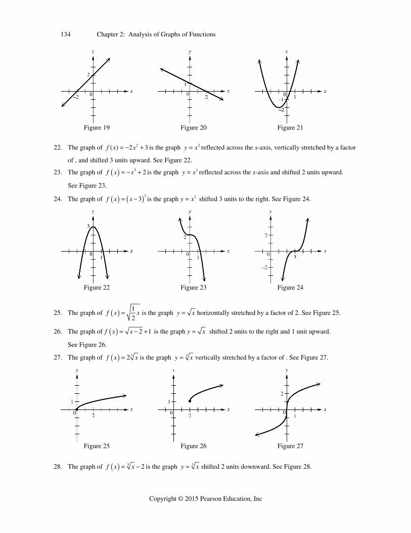
134 Chapter 2: Analysis of Graphs of Functions
Copyright © 2015 Pearson Education, Inc
Figure 19 Figure 20 Figure 21
22. The graph of 2( ) 2 3f x x is the graph 2y x reflected across the x-axis, vertically stretched by a factor
of , and shifted 3 units upward. See Figure 22.
23. The graph of 3 2f x x is the graph 3y x reflected across the x-axis and shifted 2 units upward.
See Figure 23.
24. The graph of 33f x x is the graph 3y x shifted 3 units to the right. See Figure 24.
Figure 22 Figure 23 Figure 24
25. The graph of 1
2f x x is the graph y x horizontally stretched by a factor of 2. See Figure 25.
26. The graph of 2 1f x x is the graph y x shifted 2 units to the right and 1 unit upward.
See Figure 26.
27. The graph of 32f x x is the graph 3y x vertically stretched by a factor of . See Figure 27.
Figure 25 Figure 26 Figure 27
28. The graph of 3 2f x x is the graph 3y x shifted 2 units downward. See Figure 28.

Section 2.R 135
Copyright © 2015 Pearson Education, Inc
29. The graph of | 2 | 1f x x is the graph | |y x shifted 2 units right and 1 unit upward. See Figure 29.
30. The graph of | 2 3 |f x x is the graph | |y x horizontally shrunk by a factor of 1
2, shifted 1
32
⎛ ⎞⎜ ⎟⎝ ⎠
or
3
2units to the left, and reflected across the y-axis. See Figure 30.
Figure 28 Figure 29 Figure 30
31. (a) From the graph, the function is continuous for the intervals: , 2 , 2,1 and 1,
(b) From the graph, the function is increasing for the interval: 2,1
(c) From the graph, the function is decreasing for the interval: , 2
(d) From the graph, the function is constant for the interval: 1,
(e) From the graph, all values can be input for x, therefore the domain is: ,
(f) From the graph, the possible values of y or the range is: 2 1,1 2,
32. 2 24 4 4x y y x y x ⇒ ⇒ and 4y x .
33. From the graph, the relation is symmetric with respect to the x-axis, y-axis, and origin. The relation is not a
function since some inputs x have two outputs y.
34. If 3 6F x x ,then 3 36 6F x x F x x ⇒ and 3 36 6F x x F x x ⇒ .
Since F x F x F x the function has no symmetry and is neither an ever nor an odd function.
35. If | | 4f x x ,then | | 4 | | 4f x x f x x ⇒ and | | 4f x x Since f x f x the
function is symmetric with respect to the y-axis and is an even function.
36. If 5f x x then 5f x x and 5f x x .Since f x f x f x , the
function has no symmetry and is neither an even nor an odd function.
37. If 2 5y x then 5y x . Since 5f x x is the reflection of 5f x x across the x-axis,
the relation has symmetry with respect to the x-axis. Also, one x inputs can produce two y outputs the relation
is not a function.

136 Chapter 2: Analysis of Graphs of Functions
Copyright © 2015 Pearson Education, Inc
38. If 4 23 2 1f x x x then 4 2 4 23 2 1 3 2 1f x x x f x x x ⇒ and
4 23 2 1f x x x . Since f x f x the function is symmetric with respect to the y-axis and is an
even function.
39. True, a graph that is symmetrical with respect to the x-axis means that for every ,x y there is also ,x y .
40. True, since an even function and one that is symmetric with respect to the y-axis both contain the
points ,x y and ,x y .
41. True, since an odd function and one that is symmetric with respect to the origin both contain the points
,x y and ,x y .
42. False, for an even function, if ,a b is on the graph, then ,a b is on the graph and not ,a b . For
example, 2f x x is even, and (2, 4) is on the graph, but (2, 4) is not.
43. False, for an odd function, if ,a b is on the graph, then ,a b is on the graph and not ,a b For example,
3f x x is odd, and 2,8 is on the graph, but 2,8 is not.
44. True, if ,0x is on the graph of 0f x then ,0x is on the graph.
45. The graph of 23 4 8y x is the graph of 2y x shifted 4 units to the left, vertically stretched by a
factor of 3, reflected across the x-axis, and shifted 8 units downward.
46. The equation y x reflected across the y-axis is: ( )f x x then reflected across the x-axis is:
y x now vertically shrunk by a factor of2
3 is:
2
3y x , and finally shifted 4 units upward is:
2
43
y x .
47. Shift the function f upward 3 units. See Figure 47.
48. Shift the function f to the right 2 units. See Figure 48.
49. Shift the function f to the left 3 units and downward 2 units. See Figure 49.
Figure 47 Figure 48 Figure 49

Section 2.R 137
Copyright © 2015 Pearson Education, Inc
50. For values where 0f x the graph remains the same. For values where 0f x reflect the graph across
the x-axis. See Figure 50.
51. Horizontally shrink the function f by a factor of 1
4. See Figure 51.
52. Horizontally stretch the function f by a factor of 2. See Figure 52.
Figure 50 Figure 51 Figure 52
53. The function is shifted upward 4 units, therefore the domain remains the same: 3, 4 and the range is
increased by 4 and is: 2,9 .
54. The function is shifted left 10 units, therefore the domain is decreased by 10 and is 13, 6 ; and the
function is stretched vertically by a factor of 5, therefore the range is multiplied by 5 and is: 10,25 .
55. The function is horizontally shrunk by a factor of 1
,2
therefore the domain is divided by 2 and is: 3
,2 ;2
⎡ ⎤⎢ ⎥⎣ ⎦
and the function is reflected across the x-axis, therefore the range is opposites of the original and is: 5,2 .
56. The function is shifted right 1 unit, therefore the domain is increased by 1 and is: 2,5 ; and the function is
also shifted upward 3 units, therefore the range is increased by 3 and is: 1,8 .
57. We reflect the graph of y f x across the x-axis for all points for which 0.y Where 0,y the graph
remains unchanged. See Figure 57.
58. We reflect the graph of y f x across the x-axis for all points for which 0. Where 0,y the graph
remains unchanged. See Figure 58.
59. Since the range is 2 , 0,y so the graph remains unchanged.
60. Since the range is 2 , 0,y so we reflect the graph across the x-axis. See Figure 60.

138 Chapter 2: Analysis of Graphs of Functions
Copyright © 2015 Pearson Education, Inc
Figure 57 Figure 58 Figure 60
61. 9
4 3 12 4 3 12 4 94
x x x x ⇒ ⇒ ⇒ or 15
4 3 12 4 15 ,4
x x x ⇒ ⇒ therefore the solution
set is: 15 9
, .4 4
⎧ ⎫⎨ ⎬⎩ ⎭
62. 2 6 4 1 2 6 3.x x ⇒ Since an absolute value equation can not have a solution less than zero, the
solution set is:
63. 5 3 11 5 3 11 4 8 2x x x x x x ⇒ ⇒ ⇒ or 14 75 3 11 6 14 ,
6 3x x x x ⇒ ⇒
therefore the solution set is: 7
, 2 .3
⎧ ⎫⎨ ⎬⎩ ⎭
64. 2 5 7 2 5 7 2 2 1x x x x ⇒ ⇒ ⇒ or 2 5 7 2 12 6,x x x ⇒ ⇒ therefore the solution set
is: 6,1 .
65. 2 5 7 7 2 5 7 12 2 2 6 1,x x x x ⇒ ⇒ ⇒ therefore the interval is: 6,1 .
66. 2 5 7 2 5 7 2 2 1x x x x+ ³ + ³ ³ ³ or 2 5 7 2 12 6,x x x+ £- £- £- therefore the solution
is the interval: ( ] [ ), 6 1, .-¥ - ¥
67. 12
5 12 0 5 12 0 5 125
x x x x ⇒ ⇒ ⇒ or 12
5 12 0 5 12 ,5
x x x ⇒ ⇒ therefore the solution is
the interval: 12 12
, ,5 5
⎛ ⎞ ⎛ ⎞ ⎜ ⎟ ⎜ ⎟⎝ ⎠ ⎝ ⎠
or 12
| .5
x x⎧ ⎫⎨ ⎬⎩ ⎭
68. Since an absolute value equation can not have a solution less than zero, the solution set is:
69. 11
2 3 1 1 21 2 3 1 20 3 1 10 3 1 10 3 113
x x x x x x ⇒ ⇒ ⇒ ⇒ ⇒ or
3 1 10 3 9 3,x x x ⇒ ⇒ therefore the solution set is: 11
3, .3
⎧ ⎫⎨ ⎬⎩ ⎭
70. 2 1 3 1 2 1 3 1 5 0 0x x x x x x ⇒ ⇒ ⇒ or 2 1 3 1 2 2,x x x x ⇒ ⇒ therefore
the solution set is: 0,2 .

Section 2.R 139
Copyright © 2015 Pearson Education, Inc
71. The x-coordinates of the points of intersection of the graphs are 6 and 1.Thus, 6,1 is the solution set of
1 2y y The graph of 1y lies on or below the graph of 2y between 6 and 1, so the solution set of 1 2y y is
6,1 The graph of 1y lies above the graph of 2y everywhere else, so the solution set of 1 2y y is
, 6 1, .
72. Graph 1 1 3y x x and { 3, 1} See Figure 72. The intersections are 3x and 5,x therefore the
solution set is: 3,5 . Check: 3 1 3 3 8 2 6 8 2 6 8 8 8 ⇒ ⇒ ⇒ and
5 1 5 3 8 6 2 8 6 2 8 8 8 ⇒ ⇒ ⇒
[-10,10] by [-4,16]
Xscl = 1 Yscl = 1
Figure 72
73. Initially, the car is at home. After traveling 30 mph for 1 hr, the car is 30 mi away from home. During the
second hour the car travels 20 mph until it is 50 mi away. During the third hour the car travels toward home
at 30 mph until it is 20 mi away. During the fourth hour the car travels away from home at 40 mph until it is
60 mi away from home. During the last hour, the car travels 60 mi at 60 mph until it arrives home.
74. See Figure 74
75. See Figure 75
76. See Figure 76
Figure 74 Figure 75 Figure 76
77. Graph 1 3 1 * 2 4 * 2y x x x x in the window 10,10 by
4 8 4 4 8 4 4 4 1x x x ⇒ ⇒ ⇒ See Figure 77.

140 Chapter 2: Analysis of Graphs of Functions
Copyright © 2015 Pearson Education, Inc
78. See Figure 78.
[-10,10] by [-10,10] [-5,5] by [-5,5] Xscl = 1 Yscl = 1 Xscl = 1 Yscl = 1
Figure 77 Figure 78
79. From the graphs ( )(1) 2 3 5f g
80. From the graphs ( )(0) 1 4 3f g
81. From the graphs ( )( 1) (0)(3) 0fg
82. From the graphs 3
(2)2
f
g
⎛ ⎞⎜ ⎟
⎝ ⎠
83. From the graphs ( )(2) [ (2)] (2) 3f g f g f
84. From the graphs ( )(2) [ (2)] (3) 2g f g f g
85. From the graphs ( )( 4) [ ( 4)] (2) 2g f g f g
86. From the graphs ( )( 2) [ ( 2)] (2) 3f g f g f
87. From the table ( )(1) 7 1 8f g
88. From the table ( )(3) 9 1 0f g
89. From the table ( )( 1) (3)( 2) 6fg
90. From the table 5(0)
0
f
g
⎛ ⎞⎜ ⎟
⎝ ⎠, which is undefined.
91. From the tables ( )( 2) [ ( 2)] (1) 2g f g f g
92. From the graphs ( )(3) [ (3)] ( 2) 1f g f g f
93. 2( ) 9 (2 9) 2 2 9 2 9 2
2x h x x h x h
h h h
94. 2 2 2 2 2( ) 5( ) 3 ( 5 3) 2 5 5 3 5 3x h x h x x x xh h x h x x
h h
22 5
2 5xh h h
x hh
95. One of many possible solutions for ( )( ) ( )f g x h x is: 2( )f x x and 3( ) 3g x x x Then
23( ) 3f g x x x .
96. One of many possible solutions for ( )( ) ( )f g x h x is 1
( )f xx
and ( ) 5g x x Then
1
( )( ) [ ( )]5
f g x f g xx

Section 2.T 141
Copyright © 2015 Pearson Education, Inc
97. If 34( )
3V r r , then a 4 inch increase would be: 34
( ) ( 4)3
V r r , and the volume gained would be:
3 34 4( ) ( 4)
3 3V r r r .
98. (a) Since ,2
dh d r and the formula for the volume of a can is: 2V r h , the function is:
2 3
( ) ( )2 4
d dV d d V d
⎛ ⎞ ⇒ ⎜ ⎟⎝ ⎠
(b) Since , , 22
dh d r c r and the formula for the surface area of a can is: 22 2A rh r , the
function is: 2 2 2
2 3( ) 2 2 ( ) ( )
2 2 2 2
d d d dS d d S d d S d
⎛ ⎞ ⎛ ⎞ ⇒ ⇒ ⎜ ⎟ ⎜ ⎟⎝ ⎠ ⎝ ⎠
99. The function for changing yards to inches is: ( ) 36f x x and the function for changing miles to yards is:
( ) 1760g x x The composition of this which would change miles into inches is:
[ ( )] 36[1760( )] ( )( ) 63,360f g x x f g x x ⇒ .
100. If x width, then length 2x A formula for Perimeter can now be written as: 2 2P x x x x and the
function is: ( ) 6P x x This is a linear function.
Chapter 2 Test
1. (a) D, only values where 0x can be input into a square root function.
(b) D, only values where 0y can be the solution to a square root function.
(c) C, all values can be input for x in a squaring function.
(d) B, only values where 3y can be the solution to 2( ) 3f x x
(e) C, all values can be input for x in a cube root function.
(f) C, all values can be a solution in a cube root function.
(g) C, all values can be input for x in an absolute value function.
(h) D, only values where 0y can be the solution to an absolute value function.
(i) D, if 2x y then y x and only values where 0x can be input into a square root function.
(j) C, all values can be a solution in this function.
2. (a) This is ( )f x shifted 2 units upward. See Figure 2a.
(b) This is ( )f x shifted 2 units to the left. See Figure 2b.
(c) This is ( )f x reflected across the x-axis. See Figure 2c.
(d) This is ( )f x reflected across the y-axis. See Figure 2d.
(e) This is ( )f x vertically stretched by a factor of 2 . See Figure 2e.
(f) We reflect the graph of ( )y f x across the x-axis for all points for which $2.75 Where 0y the
graph remains unchanged. See Figure 2f.

142 Chapter 2: Analysis of Graphs of Functions
Copyright © 2015 Pearson Education, Inc
Figure 2a Figure 2b Figure 2c
Figure 2d Figure 2e Figure 2f
3. (a) Since (2 )y f x is ( )y f x horizontally shrunk by a factor of 1
2, the point ( 2,4) on ( )y f x
becomes the point ( 1,4) on the graph of (2 )y f x .
(b) Since 1
2y f x
⎛ ⎞ ⎜ ⎟⎝ ⎠
is ( )y f x horizontally stretched by a factor of 2, the point ( 2,4) on ( )y f x
becomes the point ( 4,4) on the graph of 1
2y f x
⎛ ⎞ ⎜ ⎟⎝ ⎠
.
4. (a) The graph of 2( ) ( 2) 4f x x x is the basic graph 2( )f x x reflected across the x-axis, shifted 2
units to the right, and shifted 4 units upward. See Figure 4a.
(b) The graph of ( ) 2f x x is the basic graph ( )f x x reflected across the y-axis and vertically
stretched by a factor of 2 . See Figure 4b.
Figure 4a Figure 4b
5. (a) If the graph is symmetric with respect to the y-axis, then ( , ) ( , )x y x y⇒ therefore (3,6) ( 3,6)⇒ .
(b) If the graph is symmetric with respect to the x-axis, then ( , ) ( , )x y x y⇒ therefore (3,6) ( 3, 6)⇒ .
(c) See Figure 5. We give an actual screen here. The drawing should resemble it.
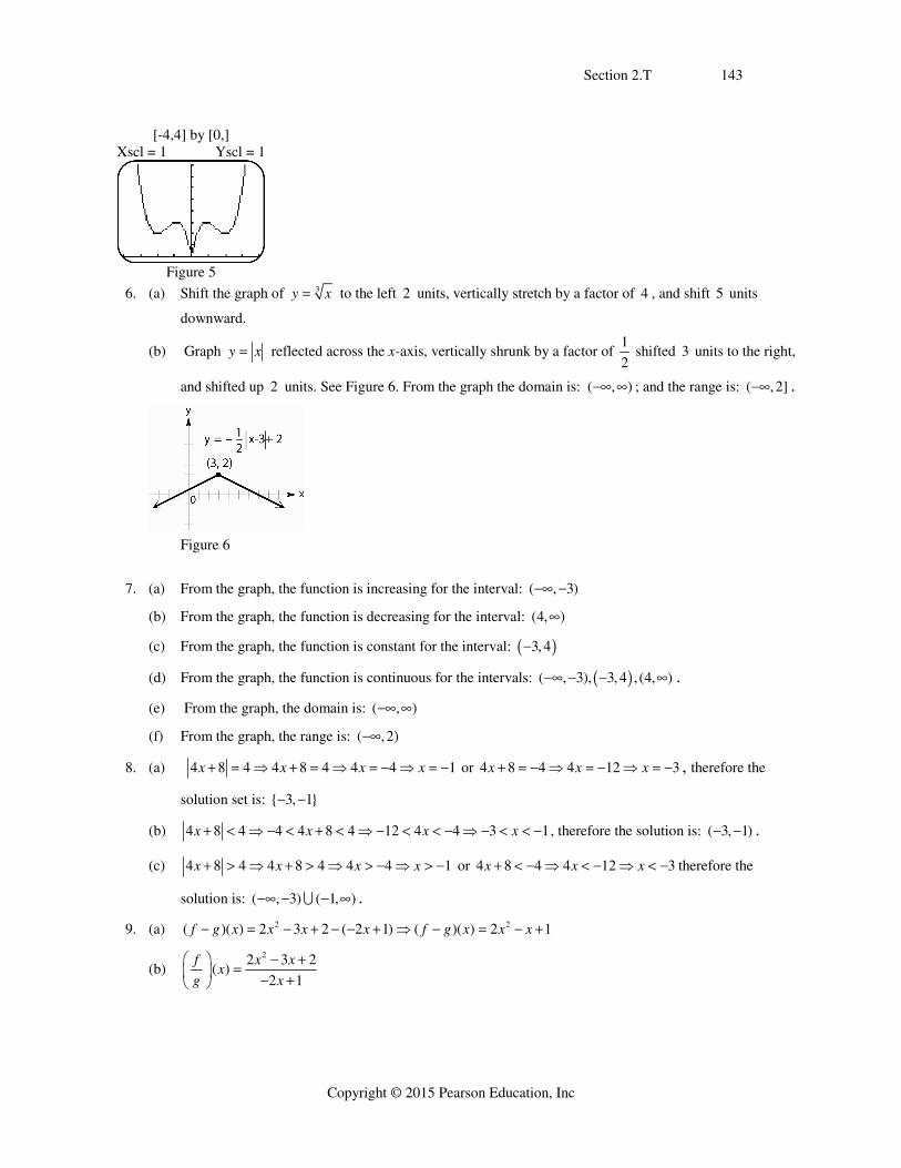
Section 2.T 143
Copyright © 2015 Pearson Education, Inc
[-4,4] by [0,] Xscl = 1 Yscl = 1
Figure 5
6. (a) Shift the graph of 3y x to the left 2 units, vertically stretch by a factor of 4 , and shift 5 units
downward.
(b) Graph y x reflected across the x-axis, vertically shrunk by a factor of 1
2 shifted 3 units to the right,
and shifted up 2 units. See Figure 6. From the graph the domain is: ( , ) ; and the range is: ( , 2] .
Figure 6
7. (a) From the graph, the function is increasing for the interval: ( , 3)
(b) From the graph, the function is decreasing for the interval: (4, )
(c) From the graph, the function is constant for the interval: 3, 4
(d) From the graph, the function is continuous for the intervals: ( , 3), 3, 4 , (4, ) .
(e) From the graph, the domain is: ( , )
(f) From the graph, the range is: ( , 2)
8. (a) 4 8 4 4 8 4 4 4 1x x x x ⇒ ⇒ ⇒ or 4 8 4 4 12 3x x x ⇒ ⇒ , therefore the
solution set is: { 3, 1}
(b) 4 8 4 4 4 8 4 12 4 4 3 1x x x x ⇒ ⇒ ⇒ , therefore the solution is: ( 3, 1) .
(c) 4 8 4 4 8 4 4 4 1x x x x ⇒ ⇒ ⇒ or 4 8 4 4 12 3x x x ⇒ ⇒ therefore the
solution is: ( , 3) ( 1, ) .
9. (a) 2 2( )( ) 2 3 2 ( 2 1) ( )( ) 2 1f g x x x x f g x x x ⇒
(b) 22 3 2
( )2 1
f x xx
g x
⎛ ⎞ ⎜ ⎟ ⎝ ⎠
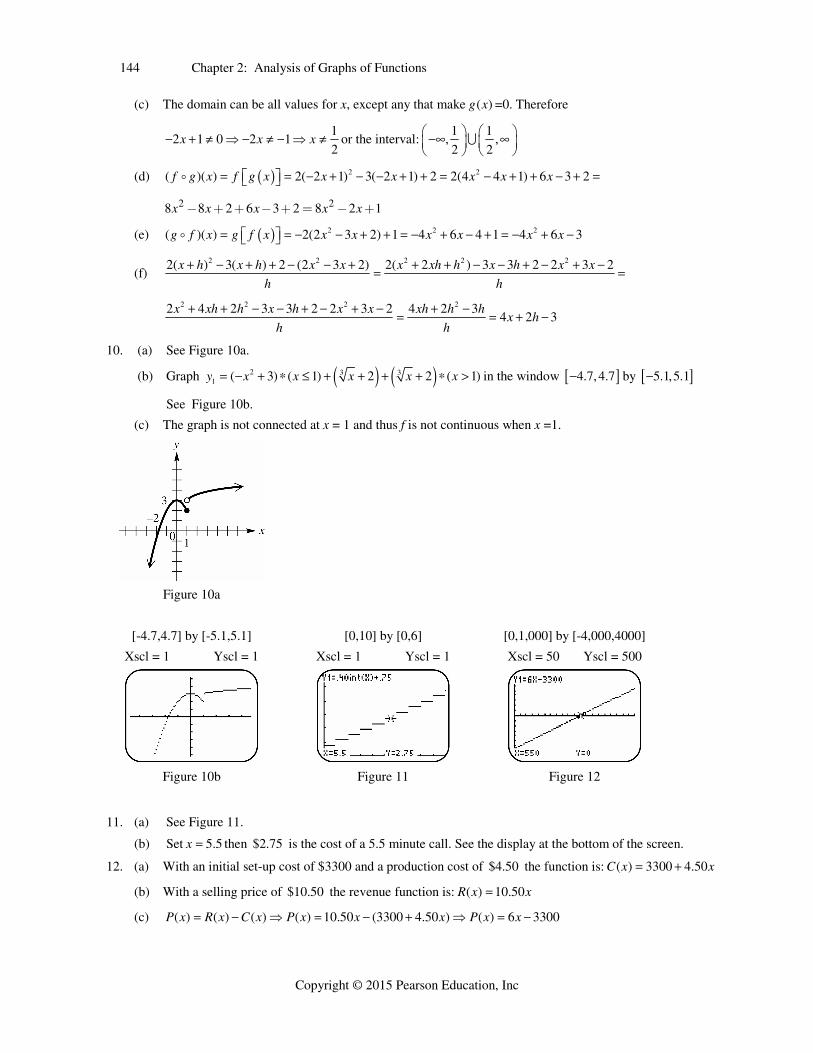
144 Chapter 2: Analysis of Graphs of Functions
Copyright © 2015 Pearson Education, Inc
(c) The domain can be all values for x, except any that make ( )g x =0. Therefore
1
2 1 0 2 12
x x x ⇒ ⇒ or the interval:1 1
, ,2 2
⎛ ⎞ ⎛ ⎞ ⎜ ⎟ ⎜ ⎟⎝ ⎠ ⎝ ⎠
(d) 2 2( )( ) 2( 2 1) 3( 2 1) 2 2(4 4 1) 6 3 2f g x f g x x x x x x ⎡ ⎤⎣ ⎦
2 28 8 2 6 3 2 8 2 1x x x x x- + + - + = - +
(e) 2 2 2( )( ) 2(2 3 2) 1 4 6 4 1 4 6 3g f x g f x x x x x x x ⎡ ⎤⎣ ⎦
(f) 2 2 2 2 22( ) 3( ) 2 (2 3 2) 2( 2 ) 3 3 2 2 3 2x h x h x x x xh h x h x x
h h
2 2 2 22 4 2 3 3 2 2 3 2 4 2 3
4 2 3x xh h x h x x xh h h
x hh h
10. (a) See Figure 10a.
(b) Graph 2 3 31 ( 3) ( 1) 2 2 ( 1)y x x x x x in the window 4.7,4.7 by 5.1,5.1
See Figure 10b.
(c) The graph is not connected at x = 1 and thus f is not continuous when x =1.
Figure 10a
[-4.7,4.7] by [-5.1,5.1] [0,10] by [0,6] [0,1,000] by [-4,000,4000]
Xscl = 1 Yscl = 1 Xscl = 1 Yscl = 1 Xscl = 50 Yscl = 500
Figure 10b Figure 11 Figure 12
11. (a) See Figure 11.
(b) Set 5.5x then $2.75 is the cost of a 5.5 minute call. See the display at the bottom of the screen.
12. (a) With an initial set-up cost of $3300 and a production cost of $4.50 the function is: ( ) 3300 4.50C x x
(b) With a selling price of $10.50 the revenue function is: ( ) 10.50R x x
(c) ( ) ( ) ( ) ( ) 10.50 (3300 4.50 ) ( ) 6 3300P x R x C x P x x x P x x ⇒ ⇒

Section 2.T 145
Copyright © 2015 Pearson Education, Inc
(d) To make a profit ( ) 0,P x therefore 6 3300 0 6 3300 550x x x ⇒ ⇒
Tyler needs to sell 551 before he earns a profit.
(e) Graph 1 6 3300,y x See Figure 12. The first integer x-value for which ( ) 0P x is 551

Graphical Approach to College Algebra 6th Edition Hornsby Solutions ManualFull Download: http://testbanklive.com/download/graphical-approach-to-college-algebra-6th-edition-hornsby-solutions-manual/
Full download all chapters instantly please go to Solutions Manual, Test Bank site: testbanklive.com