Graphical Models and Bayesian Networks

Tutorial at useR! 2014 – Los Angeles

Søren Højsgaard

Department of Mathematical Sciences

Aalborg University, Denmark

July 1, 2014

Printed: July 1, 2014 File: bayesnet-slides.tex

2

Contents1 Outline of tutorial 5

1.1 Package versions . . . . . . . . . . . . . . . . . . . . . . . . . . . . . . . . . . . 61.2 A bit of history . . . . . . . . . . . . . . . . . . . . . . . . . . . . . . . . . . . . 71.3 Book: Graphical Models with R . . . . . . . . . . . . . . . . . . . . . . . . . . . 8

2 The chest clinic narrative 102.1 DAG–based models . . . . . . . . . . . . . . . . . . . . . . . . . . . . . . . . . 122.2 DAG-based models (II) . . . . . . . . . . . . . . . . . . . . . . . . . . . . . . . 15

3 Conditional probability tables (CPTs) 16

4 An introduction to the gRain package 18

5 Querying the network 22

6 Setting evidence 23

7 The curse of dimensionality 277.1 So what is the problem? . . . . . . . . . . . . . . . . . . . . . . . . . . . . . . . 337.2 So what is the solution . . . . . . . . . . . . . . . . . . . . . . . . . . . . . . . 34

8 Message passing – a small example 358.1 Collect Evidence . . . . . . . . . . . . . . . . . . . . . . . . . . . . . . . . . . . 418.2 Distribute Evidence . . . . . . . . . . . . . . . . . . . . . . . . . . . . . . . . . 448.3 Setting evidence . . . . . . . . . . . . . . . . . . . . . . . . . . . . . . . . . . . 49

9 Message passing – the bigger picture 53

3

10 Conditional independence 58

11 Towards data 6311.1 Extracting CPTs . . . . . . . . . . . . . . . . . . . . . . . . . . . . . . . . . . . 6411.2 Extracting clique marginals . . . . . . . . . . . . . . . . . . . . . . . . . . . . . 69

12 Learning the model structure 7212.1 Contingency tables . . . . . . . . . . . . . . . . . . . . . . . . . . . . . . . . . 7312.2 Log–linear models . . . . . . . . . . . . . . . . . . . . . . . . . . . . . . . . . . 7712.3 Hierarchical log–linear models . . . . . . . . . . . . . . . . . . . . . . . . . . . 8112.4 Dependence graphs . . . . . . . . . . . . . . . . . . . . . . . . . . . . . . . . . 8212.5 The Global Markov property . . . . . . . . . . . . . . . . . . . . . . . . . . . . 8312.6 Estimation – likelihood equations . . . . . . . . . . . . . . . . . . . . . . . . . . 8412.7 Fitting log–linear models . . . . . . . . . . . . . . . . . . . . . . . . . . . . . . 8512.8 Graphical models and decomposable models . . . . . . . . . . . . . . . . . . . . 8912.9 ML estimation in decomposable models . . . . . . . . . . . . . . . . . . . . . . 92

13 Decomposable models and Bayesian networks 95

14 Testing for conditional independence 9714.1 What is a CI-test – stratification . . . . . . . . . . . . . . . . . . . . . . . . . . 9814.2 Example: University admissions . . . . . . . . . . . . . . . . . . . . . . . . . . . 100

15 Log–linear models – the gRim package 10415.1 Model specification shortcuts . . . . . . . . . . . . . . . . . . . . . . . . . . . . 10815.2 Altering graphical models . . . . . . . . . . . . . . . . . . . . . . . . . . . . . . 10915.3 Model comparison . . . . . . . . . . . . . . . . . . . . . . . . . . . . . . . . . . 11115.4 Decomposable models – deleting edges . . . . . . . . . . . . . . . . . . . . . . . 11315.5 Decomposable models – adding edges . . . . . . . . . . . . . . . . . . . . . . . 11515.6 Test for adding and deleting edges . . . . . . . . . . . . . . . . . . . . . . . . . 11715.7 Model search in log–linear models using gRim . . . . . . . . . . . . . . . . . . . 119

4

16 From graph and data to network 126

17 Prediction 129

18 Other packages 132

19 Winding up 133

5

1 Outline of tutorial

› Bayesian networks and the gRain package

› Probability propagation; conditional independence restrictionsand dependency graphs

› Learning structure with log–linear, graphical anddecomposable models for contingency tables

› Using the gRim package for structural learning.

› Convert decomposable model to Bayesian network.

› Other packages for structure learning.

6

1.1 Package versions

We shall in this tutorial use the R–packages gRbase, gRain andgRim.

Tutorial based on these development versions:> packageVersion("gRbase")[1] '1.7.0.2'> packageVersion("gRain")[1] '1.2.3.1'> packageVersion("gRim")[1] '0.1.17.1'

available at: http://people.math.aau.dk/~sorenh/software/gR

Before installing the packages above, packages from bioconductormust be installed with:> source("http://bioconductor.org/biocLite.R");> biocLite(c("graph","RBGL","Rgraphviz"))

7

1.2 A bit of history

In September 2002 a small group of people gathered in Vienna forthe brainstorming workshop “gR 2002” with the purpose ofinitiating the development of facilities in R for graphical modelling.This was made in response to the facts that:

› graphical models have now been around for a long time andhave shown to have a wide range of potential applications,

› software for graphical models is currently only available in alarge number of specialised packages, such as BUGS, CoCo,DIGRAM, MIM, TETRAD and others.

See also: http://www.ci.tuwien.ac.at/gR/gR.html andhttp://www.ci.tuwien.ac.at/Conferences/gR-2002/.

Todays workshop is one tangible result of this workshop.

8

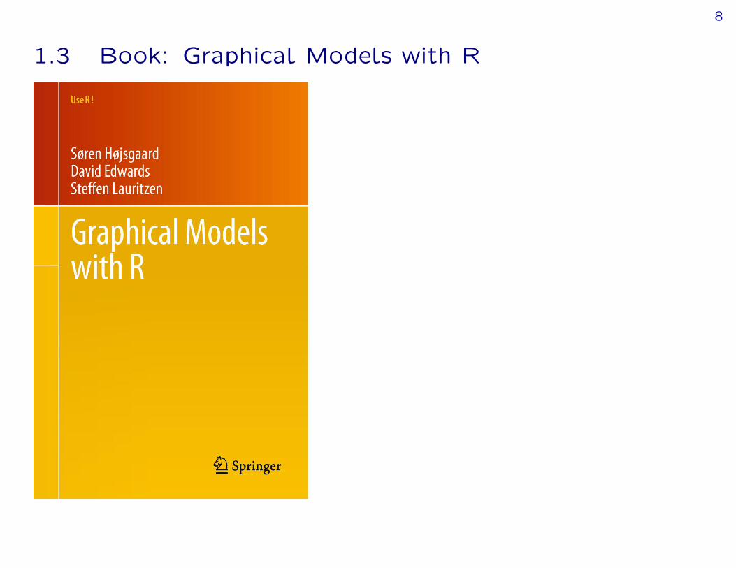
1.3 Book: Graphical Models with R

9

The book, written by some of the people who laid thefoundations of work in this area, would be ideal for researcherswho had read up on the theory of graphical models and whowanted to apply them in practice. It would also make excellentsupplementary material to accompany a course text on graphicalmodelling. I shall certainly be recommending it for use in thatrole...the book is neither a text on graphical models nor amanual for the various packages, but rather has the more modestaims of introducing the ideas of graphical modelling and thecapabilities of some of the most important packages. It succeedsadmirably in these aims. The simplicity of the commands of thepackages it uses to illustrate is apparent, as is the power of thetools available.

International Statistical Review, Volume 31, Issue 2 review byDavid J. Hand

10

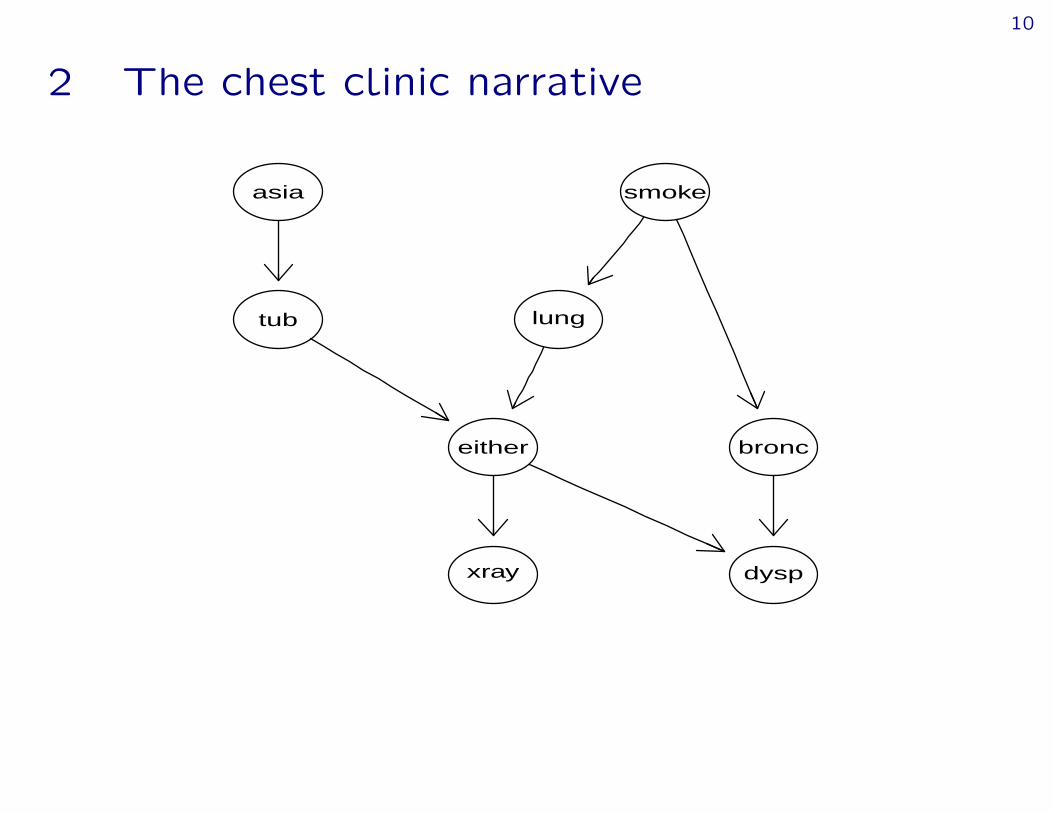
2 The chest clinic narrative

asia

tub

smoke

lung

bronceither

xray dysp

11

Lauritzen and Spiegehalter (1988) present the following narrative:

› “Shortness–of–breath (dyspnoea ) may be due totuberculosis, lung cancer or bronchitis, or none ofthem, or more than one of them.

› A recent visit to Asia increases the chances oftuberculosis, while smoking is known to be a riskfactor for both lung cancer and bronchitis.

› The results of a single chest X–ray do not discriminatebetween lung cancer and tuberculosis, as neither doesthe presence or absence of dyspnoea.”

The narrative can be pictured as a DAG (Directed Acyclic Graph)

12

2.1 DAG–based modelsasia

tub

smoke

lung

bronceither

xray dysp

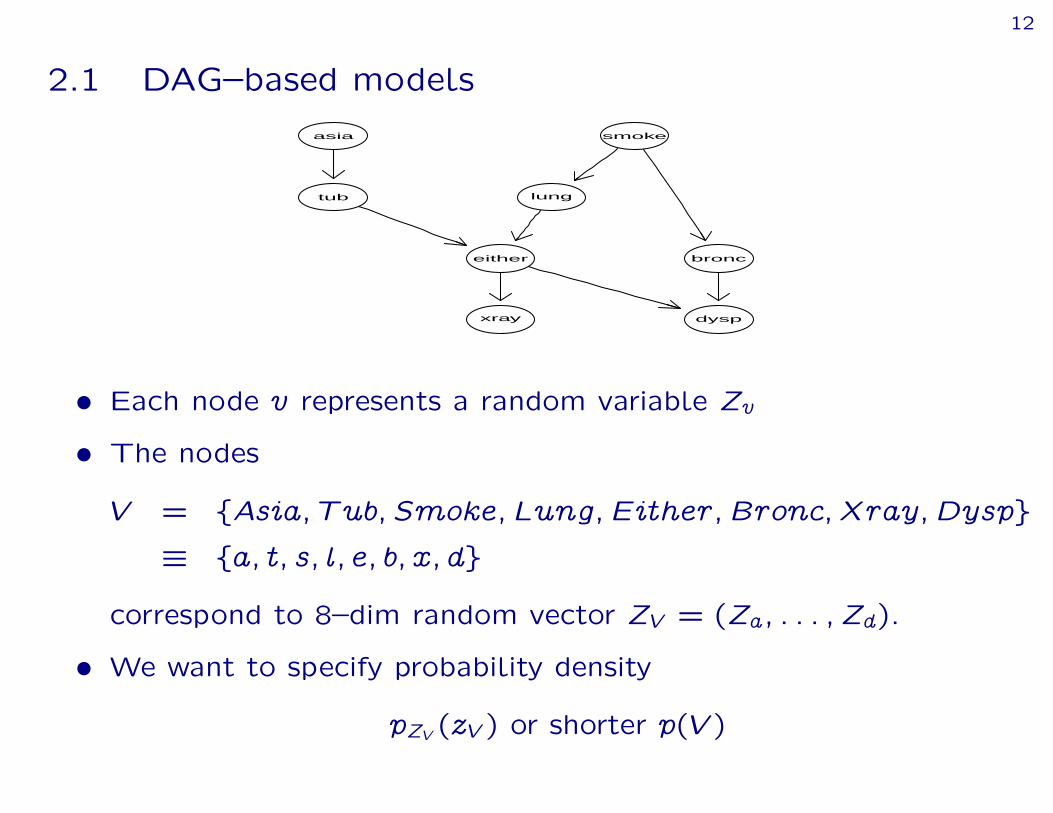
› Each node v represents a random variable Zv

› The nodes

V = fAsia; Tub; Smoke; Lung; Either; Bronc; Xray;Dyspg” fa; t; s; l; e; b; x; dg

correspond to 8–dim random vector ZV = (Za; : : : ; Zd).

› We want to specify probability density

pZV (zV ) or shorter p(V )

13

asia

tub

smoke

lung

bronceither

xray dysp

› Each node v represents a random variable Zv (here binary withlevels “yes” and “no”).

› For each combination of a node v and its parents pa(v) thereis a conditional distribution p(zvjzpa(v)), for example

pZejZt;Zl(zeitherjztub; zlung) or shorter p(ejt; l)

› Specified as a conditional probability table (a CPT), forexample for p(ejt; l) the CPT is a 2ˆ 2ˆ 2–table

14

asia

tub

smoke

lung

bronceither

xray dysp

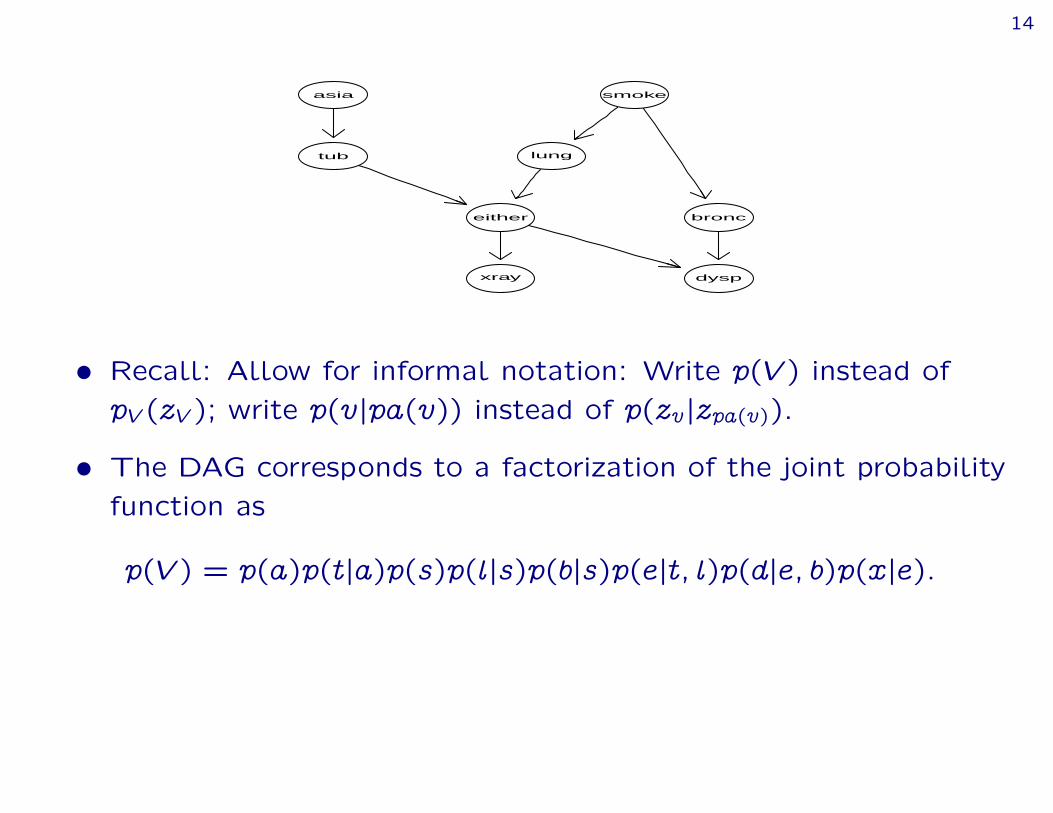
› Recall: Allow for informal notation: Write p(V ) instead ofpV (zV ); write p(vjpa(v)) instead of p(zvjzpa(v)).

› The DAG corresponds to a factorization of the joint probabilityfunction as

p(V ) = p(a)p(tja)p(s)p(ljs)p(bjs)p(ejt; l)p(dje; b)p(xje):

15

2.2 DAG-based models (II)

› More generally, a DAG with nodes V allows us to construct ajoint distribution by combining univariate conditionaldistributions, i.e.

p(V ) =Yv

p(vjpa(v))

short for p(zV ) =Qv pZvjZpa(v)(zvjzpa(v)).

› This is a powerful tool for constructing a multivariatedistribution from univariate components.

› Example: z1 ‰ N(a1; ff21), z2jz1 ‰ N(a2 + b2z1; ff22),

z3jz2 ‰ N(a3 + b3z2; ff23). Then

p((z1; z2; z3)) = p(z1)p(z2jz1)p(z3jz2)

is multivariate normal

16

3 Conditional probability tables (CPTs)

CPTs are just multiway arrays WITH dimnames attribute. Forexample p(tja):> library(gRain)> yn <- c("yes","no");> x <- c(5,95,1,99)> # Vanilla R> t.a <- array(x, dim=c(2,2), dimnames=list(tub=yn,asia=yn))> t.a

asiatub yes no

yes 5 1no 95 99

> # Alternative specification: parray() from gRbase> t.a <- parray(c("tub","asia"), levels=list(yn,yn), values=x)> t.a

asiatub yes no

yes 5 1no 95 99

17

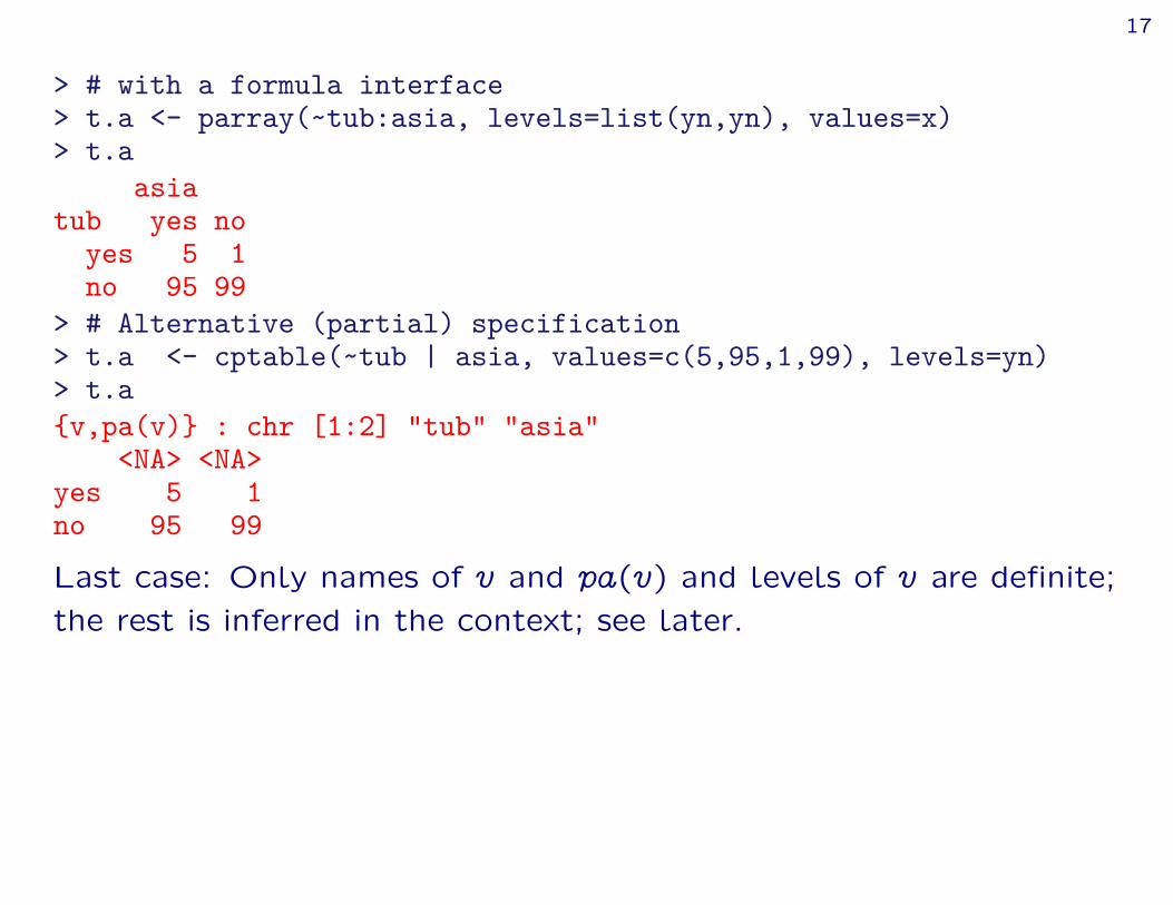
> # with a formula interface> t.a <- parray(~tub:asia, levels=list(yn,yn), values=x)> t.a

asiatub yes no

yes 5 1no 95 99

> # Alternative (partial) specification> t.a <- cptable(~tub | asia, values=c(5,95,1,99), levels=yn)> t.a{v,pa(v)} : chr [1:2] "tub" "asia"

<NA> <NA>yes 5 1no 95 99

Last case: Only names of v and pa(v) and levels of v are definite;the rest is inferred in the context; see later.

18

4 An introduction to the gRain package

Specify chest clinic network. Can be done in many ways; one isfrom a list of CPTs:> library(gRain)> yn <- c("yes","no")> a <- cptable(~asia, values=c(1,99), levels=yn)> t.a <- cptable(~tub | asia, values=c(5,95,1,99), levels=yn)> s <- cptable(~smoke, values=c(5,5), levels=yn)> l.s <- cptable(~lung | smoke, values=c(1,9,1,99), levels=yn)> b.s <- cptable(~bronc | smoke, values=c(6,4,3,7), levels=yn)> e.lt <- cptable(~either | lung:tub,values=c(1,0,1,0,1,0,0,1),

levels=yn)> x.e <- cptable(~xray | either, values=c(98,2,5,95), levels=yn)> d.be <- cptable(~dysp | bronc:either, values=c(9,1,7,3,8,2,1,9),

levels=yn)

19

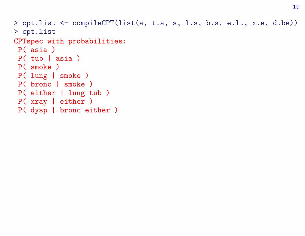
> cpt.list <- compileCPT(list(a, t.a, s, l.s, b.s, e.lt, x.e, d.be))> cpt.listCPTspec with probabilities:P( asia )P( tub | asia )P( smoke )P( lung | smoke )P( bronc | smoke )P( either | lung tub )P( xray | either )P( dysp | bronc either )

20

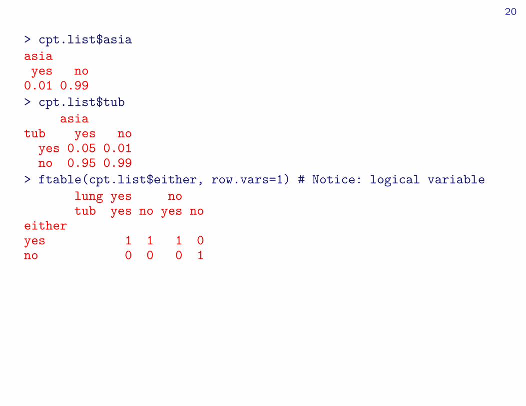
> cpt.list$asiaasiayes no

0.01 0.99> cpt.list$tub

asiatub yes no

yes 0.05 0.01no 0.95 0.99

> ftable(cpt.list$either, row.vars=1) # Notice: logical variablelung yes notub yes no yes no

eitheryes 1 1 1 0no 0 0 0 1

21

> # Create network from CPT list:> bnet <- grain(cpt.list)> # Compile network (details follow)> bnet <- compile(bnet)> bnetIndependence network: Compiled: TRUE Propagated: FALSE

Nodes: chr [1:8] "asia" "tub" "smoke" "lung" "bronc" ...

22

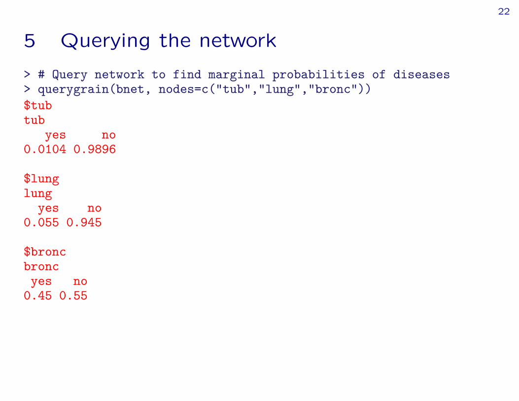
5 Querying the network

> # Query network to find marginal probabilities of diseases> querygrain(bnet, nodes=c("tub","lung","bronc"))$tubtub

yes no0.0104 0.9896

$lunglung

yes no0.055 0.945

$broncbroncyes no

0.45 0.55

23

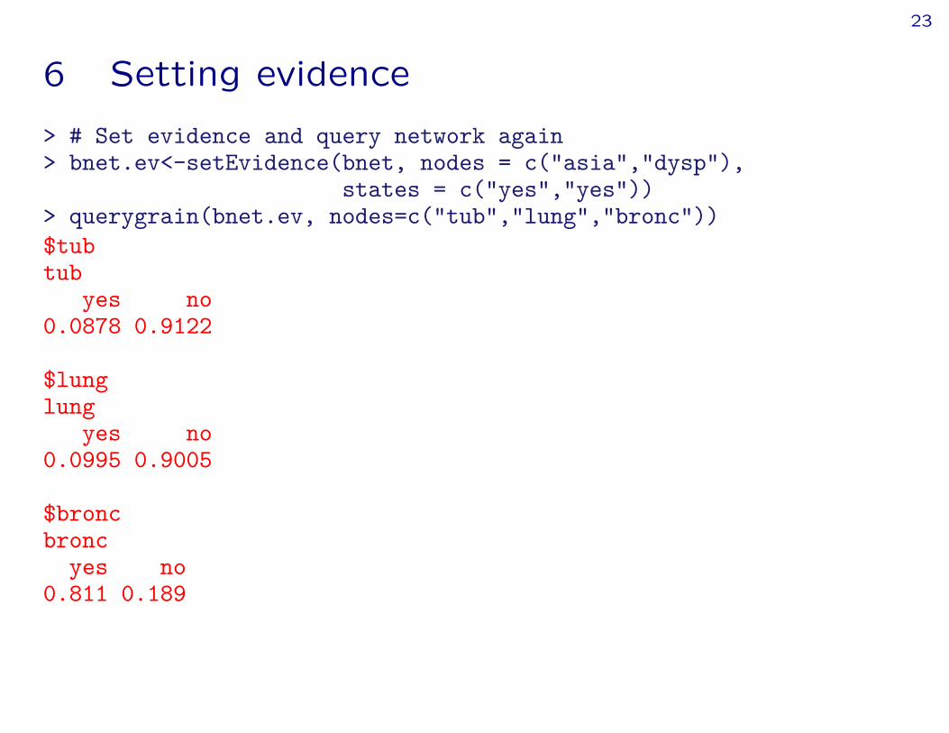
6 Setting evidence

> # Set evidence and query network again> bnet.ev<-setEvidence(bnet, nodes = c("asia","dysp"),

states = c("yes","yes"))> querygrain(bnet.ev, nodes=c("tub","lung","bronc"))$tubtub

yes no0.0878 0.9122

$lunglung

yes no0.0995 0.9005

$broncbronc

yes no0.811 0.189

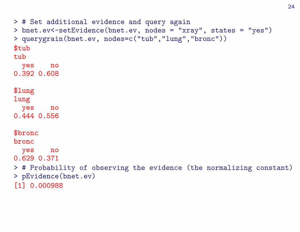
24

> # Set additional evidence and query again> bnet.ev<-setEvidence(bnet.ev, nodes = "xray", states = "yes")> querygrain(bnet.ev, nodes=c("tub","lung","bronc"))$tubtub

yes no0.392 0.608

$lunglung

yes no0.444 0.556

$broncbronc

yes no0.629 0.371> # Probability of observing the evidence (the normalizing constant)> pEvidence(bnet.ev)[1] 0.000988

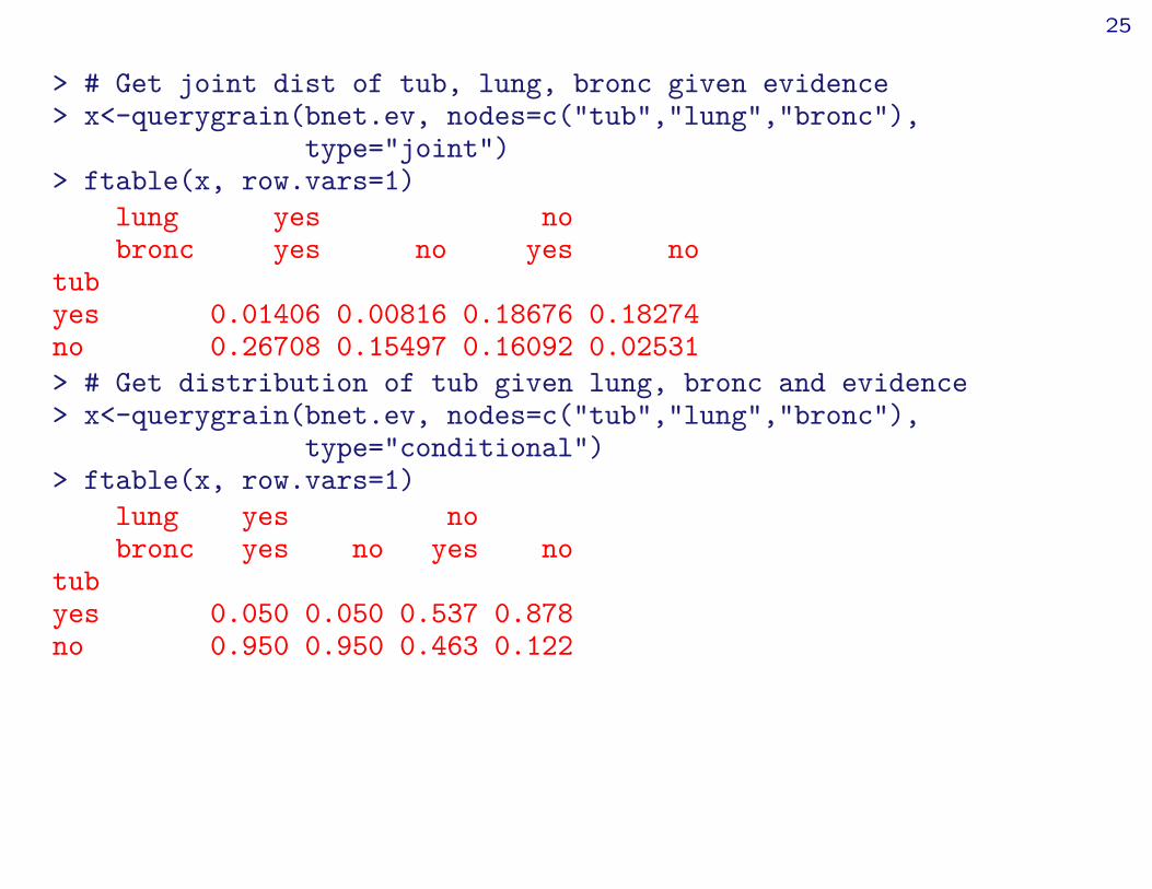
25

> # Get joint dist of tub, lung, bronc given evidence> x<-querygrain(bnet.ev, nodes=c("tub","lung","bronc"),

type="joint")> ftable(x, row.vars=1)

lung yes nobronc yes no yes no

tubyes 0.01406 0.00816 0.18676 0.18274no 0.26708 0.15497 0.16092 0.02531> # Get distribution of tub given lung, bronc and evidence> x<-querygrain(bnet.ev, nodes=c("tub","lung","bronc"),

type="conditional")> ftable(x, row.vars=1)

lung yes nobronc yes no yes no

tubyes 0.050 0.050 0.537 0.878no 0.950 0.950 0.463 0.122

26

> # Remove evidence> bnet.ev<-retractEvidence(bnet.ev, nodes="asia")> bnet.evIndependence network: Compiled: TRUE Propagated: TRUE

Nodes: chr [1:8] "asia" "tub" "smoke" "lung" "bronc" ...Findings: chr [1:2] "dysp" "xray"

27

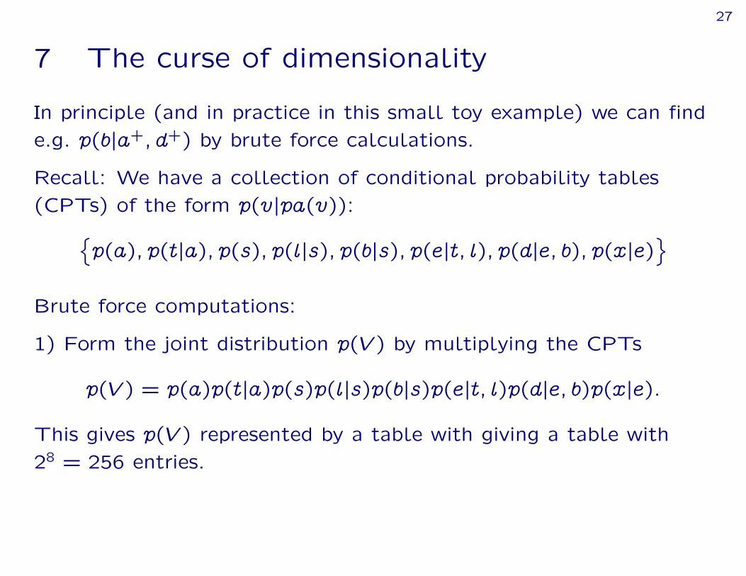
7 The curse of dimensionality

In principle (and in practice in this small toy example) we can finde.g. p(bja+; d+) by brute force calculations.

Recall: We have a collection of conditional probability tables(CPTs) of the form p(vjpa(v)):n

p(a); p(tja); p(s); p(ljs); p(bjs); p(ejt; l); p(dje; b); p(xje)o

Brute force computations:

1) Form the joint distribution p(V ) by multiplying the CPTs

p(V ) = p(a)p(tja)p(s)p(ljs)p(bjs)p(ejt; l)p(dje; b)p(xje):

This gives p(V ) represented by a table with giving a table with28 = 256 entries.

28

2) Find the marginal distribution p(a; b; d) by marginalizingp(V ) = p(a; t; s; k; e; b; x; d)

p(a; b; d) =X

t;s;k;e;b;x

p(t; s; k; e; b; x; d)

This is table with 23 = 8 entries.

3) Lastly notice that p(bja+; d+) / p(a+; b; d+).

Hence from p(a; b; d) we must extract those entries consistent witha = a+ and d = d+ and normalize the result.

Alternatively (and easier): Set all entries not consistent witha = a+ and d = d+ in p(a; b; d) equal to zero.

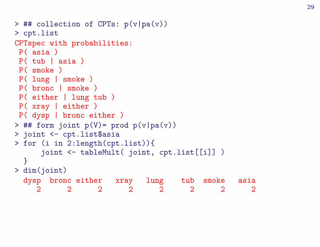
29

> ## collection of CPTs: p(v|pa(v))> cpt.listCPTspec with probabilities:P( asia )P( tub | asia )P( smoke )P( lung | smoke )P( bronc | smoke )P( either | lung tub )P( xray | either )P( dysp | bronc either )

> ## form joint p(V)= prod p(v|pa(v))> joint <- cpt.list$asia> for (i in 2:length(cpt.list)){

joint <- tableMult( joint, cpt.list[[i]] )}

> dim(joint)dysp bronc either xray lung tub smoke asia

2 2 2 2 2 2 2 2

30

> head( as.data.frame.table( joint ) )dysp bronc either xray lung tub smoke asia Freq

1 yes yes yes yes yes yes yes yes 1.32e-052 no yes yes yes yes yes yes yes 1.47e-063 yes no yes yes yes yes yes yes 6.86e-064 no no yes yes yes yes yes yes 2.94e-065 yes yes no yes yes yes yes yes 0.00e+006 no yes no yes yes yes yes yes 0.00e+00

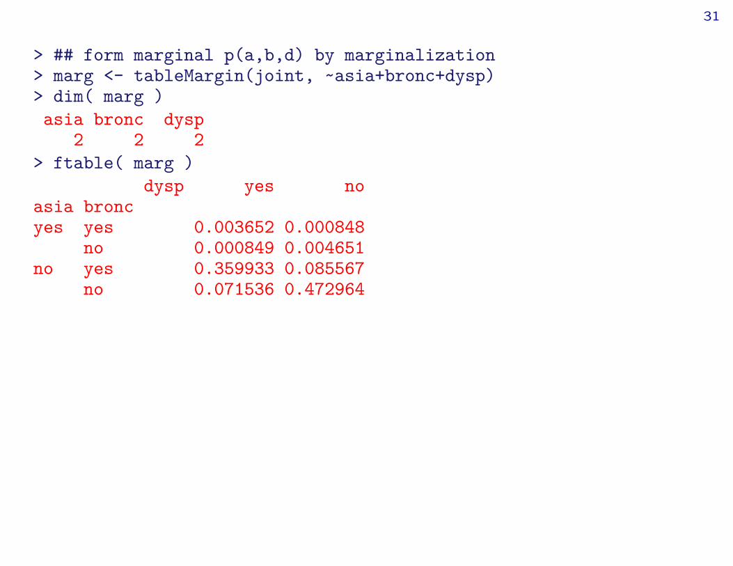
31

> ## form marginal p(a,b,d) by marginalization> marg <- tableMargin(joint, ~asia+bronc+dysp)> dim( marg )asia bronc dysp

2 2 2> ftable( marg )

dysp yes noasia broncyes yes 0.003652 0.000848

no 0.000849 0.004651no yes 0.359933 0.085567

no 0.071536 0.472964

32

> ## Set entries not consistent with asia=yes and dysp=yes> ## equal to zero> marg <- tableSetSliceValue(marg, c("asia","dysp"), c("yes","yes"),

complement=T)> ftable(marg)

dysp yes noasia broncyes yes 0.003652 0.000000

no 0.000849 0.000000no yes 0.000000 0.000000

no 0.000000 0.000000> result <- tableMargin(marg, ~bronc);> result <- result / sum( result ); resultbronc

yes no0.811 0.189

33

7.1 So what is the problem?

In chest clinic example the joint state space is 28 = 256.

If there are 80 variables each with 10 levels, the joint state space is1080 which is one of the estimates of the number of atoms in theuniverse!

Still, gRain has been succesfully used in a genetics network with80:000 nodes... How can this happen?

34

7.2 So what is the solution

The trick is NOT to calculate the joint distribution

p(V ) = p(a)p(tja)p(s)p(ljs)p(bjs)p(ejt; l)p(dje; b)p(xje):

explicitly because that leads to working with high dimensionaltables.

Instead we work on low dimensional tables and “send messages”between them.

With such a message passing scheme, all computations can bemade locally.

The challenge is to organize these local computations.

35

8 Message passing – a small example

> require(gRbase); require(Rgraphviz)> d<-dag( ~smoke + bronc|smoke + dysp|bronc ); plot(d)

smoke

bronc

dysp

36

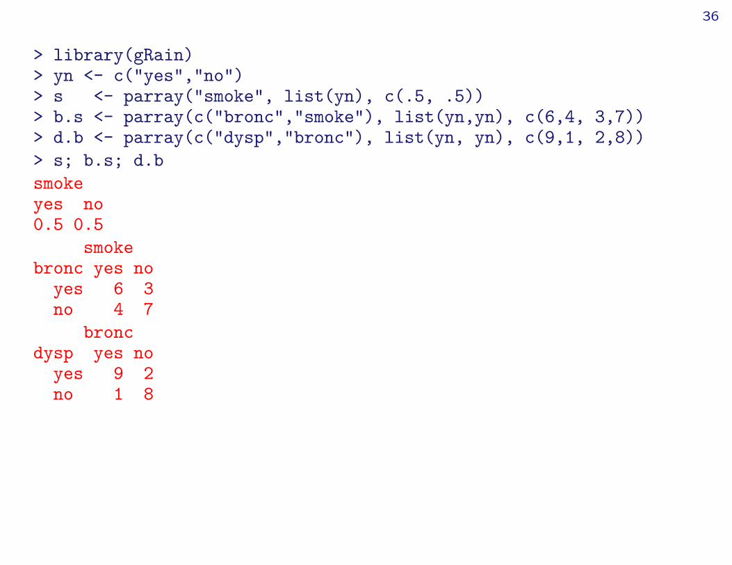
> library(gRain)> yn <- c("yes","no")> s <- parray("smoke", list(yn), c(.5, .5))> b.s <- parray(c("bronc","smoke"), list(yn,yn), c(6,4, 3,7))> d.b <- parray(c("dysp","bronc"), list(yn, yn), c(9,1, 2,8))> s; b.s; d.bsmokeyes no0.5 0.5

smokebronc yes no

yes 6 3no 4 7

broncdysp yes no

yes 9 2no 1 8

37

Recall that the joint distribution is

p(s; b; d) = p(s)p(bjs)p(djb)

i.e.> joint <- tableMult( tableMult(s, b.s), d.b) ; ftable(joint)

smoke yes nodysp broncyes yes 27.0 13.5

no 4.0 7.0no yes 3.0 1.5

no 16.0 28.0

but we really do not want to calculate this in general; here we justdo it as “proof of concept”.

38

From now on we no longer need the DAG. Instead we use anundirected graph to dictate the message passing:

The “moral graph” is obtained by 1) marrying parents and 2)dropping directions. The moral graph is (in this case) triangulatedwhich means that the cliques can be organized in a tree called ajunction tree.> dm <-moralize(d);> jtree<-ug(~smoke.bronc:bronc.dysp);> par(mfrow=c(1,3)); plot(d); plot(dm); plot(jtree)

smoke

bronc

dysp

smoke

bronc

dysp

smoke.bronc

bronc.dysp

39

> par(mfrow=c(1,3)); plot(d); plot(dm); plot(jtree)

smoke

bronc

dysp

smoke

bronc

dysp

smoke.bronc

bronc.dysp

Define q1(s; b) = p(s)p(bjs) and q2(b; d) = p(djb) and we have

p(s; b; d) = p(s)p(bjs)p(djb) = q1(s; b)q2(b; d)

We see that the q–functions are defined on the cliques of the moralgraph or - equivalently - on the nodes of the junction tree.

The q–functions are called potentials; they are non–negativefunctions but they are typically not probabilities and they are hencedifficult to interpret.

We can think of the q–functions as interactions.

40

> q1.sb <- tableMult(s, b.s); q1.sbsmoke

bronc yes noyes 3 1.5no 2 3.5

> q2.bd <- d.b; q2.bdbronc

dysp yes noyes 9 2no 1 8

The factorization

p(s; b; d) = q1(s; b)q2(b; d)

is called a clique potential representation.

Goal: We shall operate on q–functions such that at the end theywill contain the marginal distributions, i.e.

q1(s; b) = p(s; b); q2(b; d) = p(b; d)

41

8.1 Collect Evidence> plot( jtree )

smoke.bronc

bronc.dysp

We pick any node, say (b; d) as root in the junction tree, and workinwards towards the root as follows.

First, define q1(b) Ps q1(s; b).

42

> q1.b <- tableMargin(q1.sb, "bronc"); q1.bbroncyes no4.5 5.5

We have

p(s; b; d) = q1(s; b)q2(b; d) =hq1(s; b)q1(b)

ihq2(b; d)q1(b)

i

Therefore, if we update potentials as

q1(s; b) q1(s; b)=q1(b); q2(b; d) q2(b; d)q1(b)

and we obtain new potentials defined on the cliques of the junctiontree. We still have

p(s; b; d) = q1(s; b)q2(b; d)

43

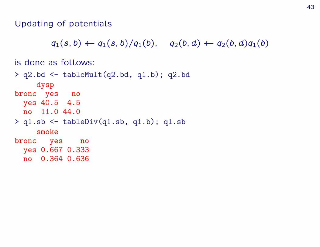
Updating of potentials

q1(s; b) q1(s; b)=q1(b); q2(b; d) q2(b; d)q1(b)

is done as follows:> q2.bd <- tableMult(q2.bd, q1.b); q2.bd

dyspbronc yes no

yes 40.5 4.5no 11.0 44.0

> q1.sb <- tableDiv(q1.sb, q1.b); q1.sbsmoke

bronc yes noyes 0.667 0.333no 0.364 0.636

44

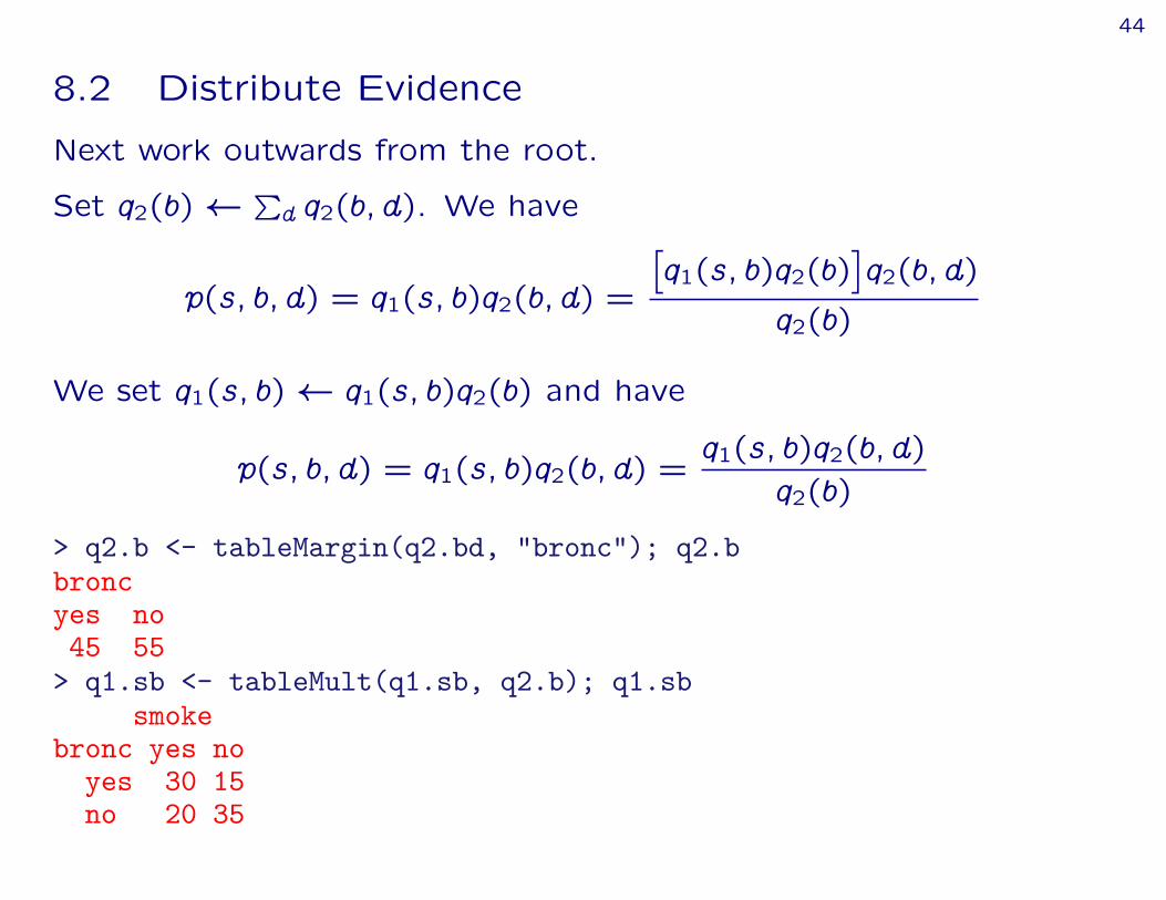
8.2 Distribute Evidence

Next work outwards from the root.

Set q2(b) Pd q2(b; d). We have

p(s; b; d) = q1(s; b)q2(b; d) =

hq1(s; b)q2(b)

iq2(b; d)

q2(b)

We set q1(s; b) q1(s; b)q2(b) and have

p(s; b; d) = q1(s; b)q2(b; d) =q1(s; b)q2(b; d)

q2(b)

> q2.b <- tableMargin(q2.bd, "bronc"); q2.bbroncyes no45 55

> q1.sb <- tableMult(q1.sb, q2.b); q1.sbsmoke

bronc yes noyes 30 15no 20 35

45

The form

p(s; b; d) = q1(s; b)q2(b; d) =q1(s; b)q2(b; d)

q2(b)

is called the clique marginal representation and the main point isnow that

q1(s; b) = p(s; b); q2(b; d) = p(b; d)

and q1 and q2 “fit on their marginals”, i.e. q1(b) = q2(b)

46

Recall that the joint distribution is> joint, , smoke = yes

broncdysp yes no

yes 27 4no 3 16

, , smoke = no

broncdysp yes no

yes 13.5 7no 1.5 28

47

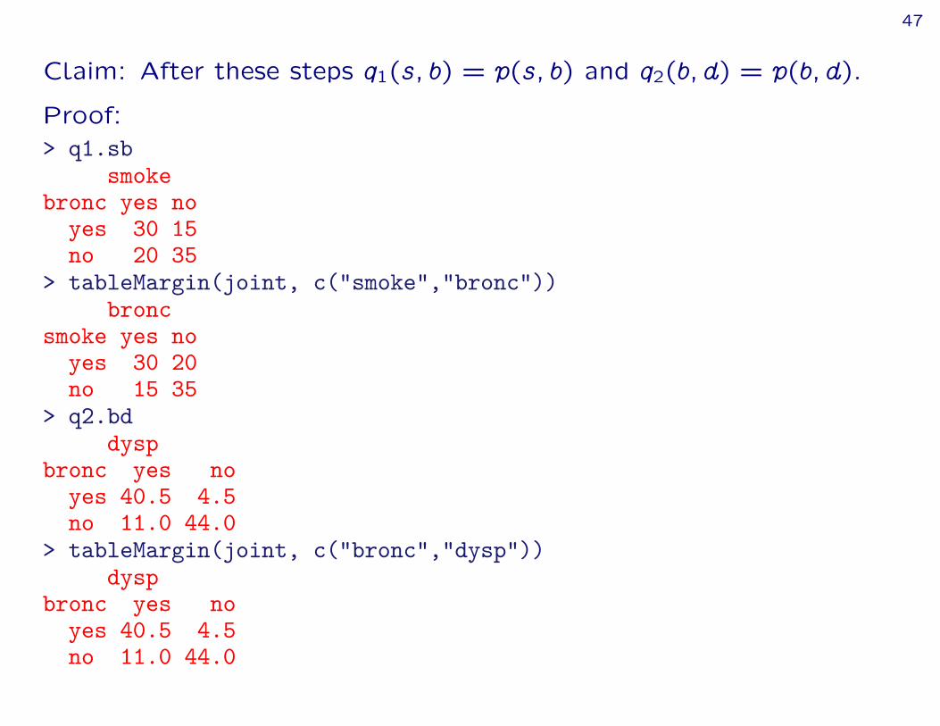
Claim: After these steps q1(s; b) = p(s; b) and q2(b; d) = p(b; d).

Proof:> q1.sb

smokebronc yes no

yes 30 15no 20 35

> tableMargin(joint, c("smoke","bronc"))bronc

smoke yes noyes 30 20no 15 35

> q2.bddysp

bronc yes noyes 40.5 4.5no 11.0 44.0

> tableMargin(joint, c("bronc","dysp"))dysp

bronc yes noyes 40.5 4.5no 11.0 44.0

48

Now we can obtain, e.g. p(b) as> tableMargin(q1.sb, "bronc") # orbroncyes no45 55

> tableMargin(q2.bd, "bronc")broncyes no45 55

And we NEVER calculated the full joint distribution!

49

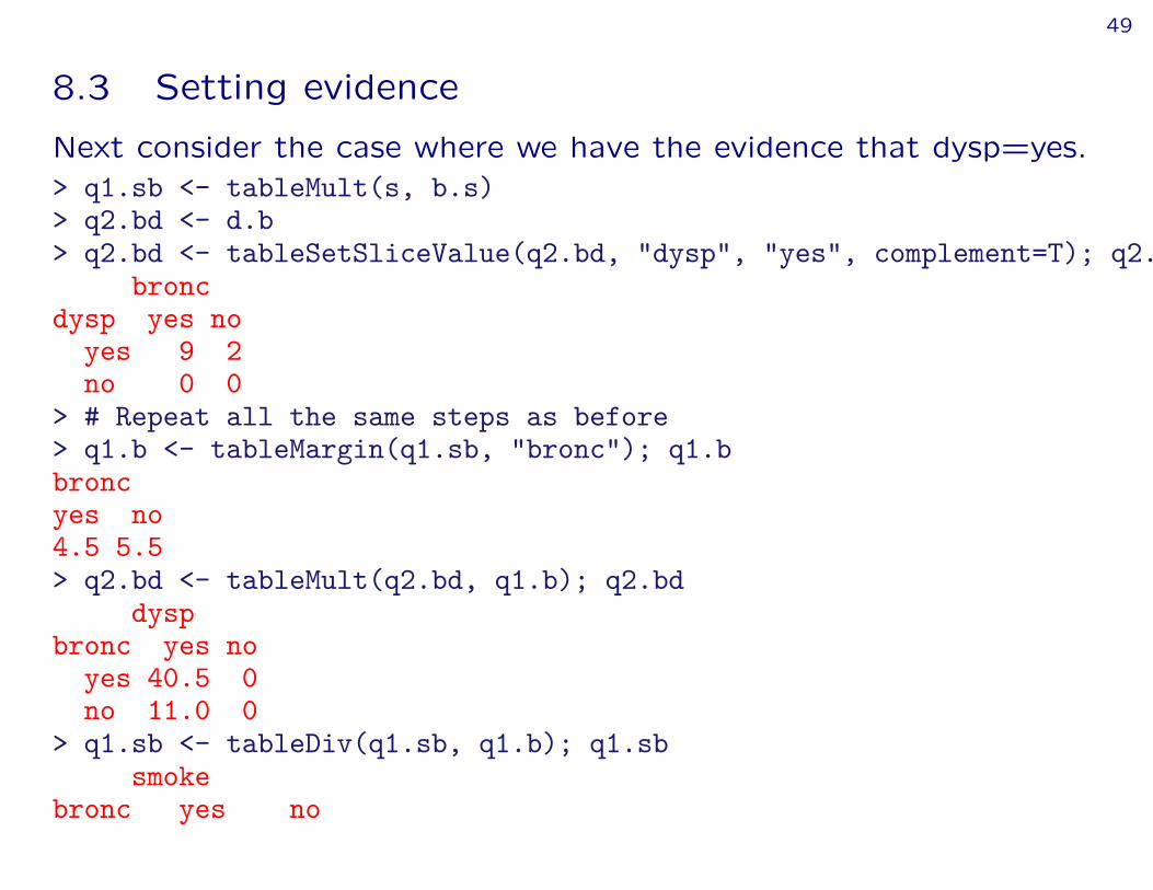
8.3 Setting evidence

Next consider the case where we have the evidence that dysp=yes.> q1.sb <- tableMult(s, b.s)> q2.bd <- d.b> q2.bd <- tableSetSliceValue(q2.bd, "dysp", "yes", complement=T); q2.bd

broncdysp yes no

yes 9 2no 0 0

> # Repeat all the same steps as before> q1.b <- tableMargin(q1.sb, "bronc"); q1.bbroncyes no4.5 5.5> q2.bd <- tableMult(q2.bd, q1.b); q2.bd

dyspbronc yes no

yes 40.5 0no 11.0 0

> q1.sb <- tableDiv(q1.sb, q1.b); q1.sbsmoke

bronc yes no

50

yes 0.667 0.333no 0.364 0.636

> q2.b <- tableMargin(q2.bd, "bronc"); q2.bbroncyes no

40.5 11.0> q1.sb <- tableMult(q1.sb, q2.b); q1.sb

smokebronc yes no

yes 27 13.5no 4 7.0

51

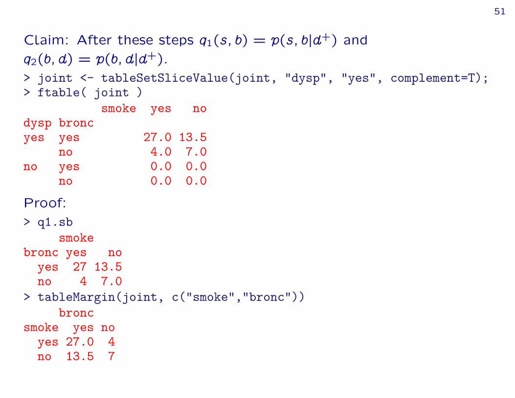
Claim: After these steps q1(s; b) = p(s; bjd+) andq2(b; d) = p(b; djd+).> joint <- tableSetSliceValue(joint, "dysp", "yes", complement=T);> ftable( joint )

smoke yes nodysp broncyes yes 27.0 13.5

no 4.0 7.0no yes 0.0 0.0

no 0.0 0.0

Proof:> q1.sb

smokebronc yes no

yes 27 13.5no 4 7.0

> tableMargin(joint, c("smoke","bronc"))bronc

smoke yes noyes 27.0 4no 13.5 7

52

> q2.bddysp

bronc yes noyes 40.5 0no 11.0 0

> tableMargin(joint, c("bronc","dysp"))dysp

bronc yes noyes 40.5 0no 11.0 0

And we NEVER calculated the full joint distribution!

53

9 Message passing – the bigger picture

The DAG is only used in connection with specifying the network;afterwards all computations are based on properties of a derivedundirected graph.

Recall goal: Avoid working with high dimensional tables.

Think of the CPTs as potentials/interactions (q-functions):

p(V ) = p(a)p(tja)p(s)p(ljs)p(bjs)p(ejt; l)p(dje; b)p(xje)

= q(a)q(t; a)q(s)q(l; s)q(b; s)q(e; t; l)q(d; e; b)q(x; e):

Notice: q–functions that are “contained” in other q–functions canbe absorbed into these; we set q(t; a) q(t; a)q(a) andq(l; s) q(l; s)q(s):

p(V ) = q(t; a)q(l; s)q(b; s)q(e; t; l)q(d; e; b)q(x; e):

54

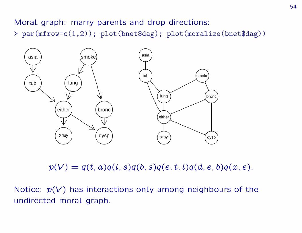
Moral graph: marry parents and drop directions:> par(mfrow=c(1,2)); plot(bnet$dag); plot(moralize(bnet$dag))

asia

tub

smoke

lung

bronceither

xray dysp

asia

tub smoke

lung bronc

either

xray dysp

p(V ) = q(t; a)q(l; s)q(b; s)q(e; t; l)q(d; e; b)q(x; e):

Notice: p(V ) has interactions only among neighbours of theundirected moral graph.

55

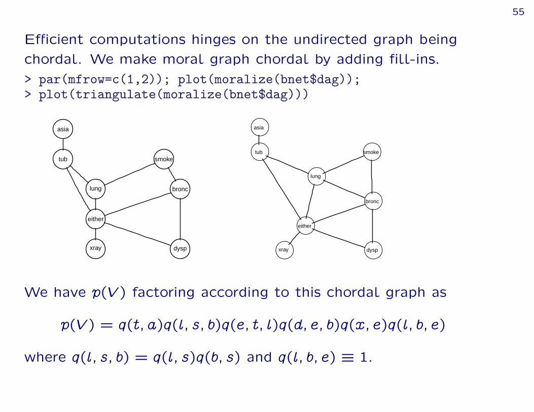
Efficient computations hinges on the undirected graph beingchordal. We make moral graph chordal by adding fill-ins.> par(mfrow=c(1,2)); plot(moralize(bnet$dag));> plot(triangulate(moralize(bnet$dag)))

asia

tub smoke

lung bronc

either

xray dysp

●asia

●tub ●smoke

●lung

●bronc

●either

●xray ●dysp

We have p(V ) factoring according to this chordal graph as

p(V ) = q(t; a)q(l; s; b)q(e; t; l)q(d; e; b)q(x; e)q(l; b; e)

where q(l; s; b) = q(l; s)q(b; s) and q(l; b; e) ” 1.

56

We have p(V ) =QC:cliques q(C).

We want to manipulate the q–functions such that p(C) = q(C)

without creating high–dimensional tables.

The manipulations are of the form (where S C)

q(S) =XCnS

q(C); q(C) q(C)~q(S); q(C) q(C)=~q(S);

Cliques of chordal graph can be ordered such that

Bk = (C1[; : : : ;[Ck`1); Sk = Bk \ Ck Cj for some j < k

so after computing q(Sk) =PCknSk q(Ck) we can absorb q(Sk) into

a Cj by q(Cj)q(Sk) which will still be a function of Cj only.

57

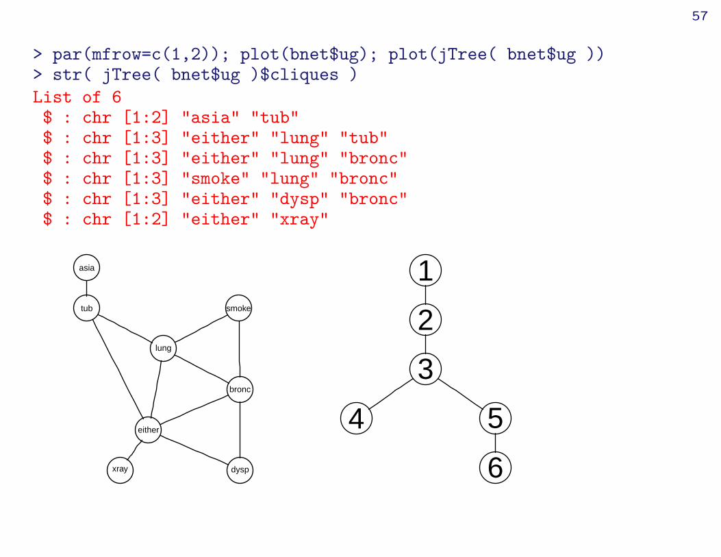
> par(mfrow=c(1,2)); plot(bnet$ug); plot(jTree( bnet$ug ))> str( jTree( bnet$ug )$cliques )List of 6$ : chr [1:2] "asia" "tub"$ : chr [1:3] "either" "lung" "tub"$ : chr [1:3] "either" "lung" "bronc"$ : chr [1:3] "smoke" "lung" "bronc"$ : chr [1:3] "either" "dysp" "bronc"$ : chr [1:2] "either" "xray"

asia

tub smoke

lung

bronc

either

xray dysp

1

2

3

4 5

6

58

10 Conditional independence

Consider again the toy example:> plot(dag(~smoke+bronc|smoke+dysp|bronc))

smoke

bronc

dysp

withp(s; b; d) = p(s)p(bjs)p(djb)

59

The factorization implies a conditional independence restriction:

p(sjb; d) = p(sjb)

Consider p(sjb; d):

p(sjb; d) = p(s)p(bjs)p(djb)Ps p(s)p(bjs)p(djb)

=p(s)p(bjs)Ps p(s)p(bjs)

On the other hand:

p(sjb) = p(s; b)

p(b)=

Pd p(s)p(bjs)p(djb)Pds p(s)p(bjs)p(djb)

=p(s)p(bjs)Ps p(s)p(bjs)

We say that “s is independent of d given b” or that “s and d areconditionally independent given b” and write s?? djb.

If we know b then getting to know also b provides no additionalinformation about s.

60

Conditional independence can often be deduced easier as follows:Suppose that for non–negative functions q1() and q2(),

p(s; b; d) = q1(s; b)q2(b; d)

Then

p(sjb; d) = q1(s; b)q2(b; d)Ps q1(s; b)q2(b; d)

=q1(s; b)Ps q1(s; b)

which is a function of s and b but not of d. So s?? djb. This iscalled the “factorisation criterion”

61

Clear that s?? djb under all these models:> par(mfrow = c(1,4))> plot(dag(~smoke+bronc|smoke+dysp|bronc))> plot(dag(~bronc+smoke|bronc+dysp|bronc))> plot(dag(~dysp+smoke|bronc+bronc|dysp))> plot(ug(~smoke:bronc+bronc:dysp))

smoke

bronc

dysp

bronc

smoke dysp

dysp

smoke

bronc

smoke

bronc

dysp

The general “rule” is therefore that separation in a graphcorresponds to conditional independence – but there is an exception

62

> plot(dag( ~smoke + dysp + bronc|smoke:dysp ))

smoke dysp

bronc

corresponding to

p(s; b; d) = p(s)p(d)p(bjs; d)

No factorization – and no conditional independence.

63

11 Towards data

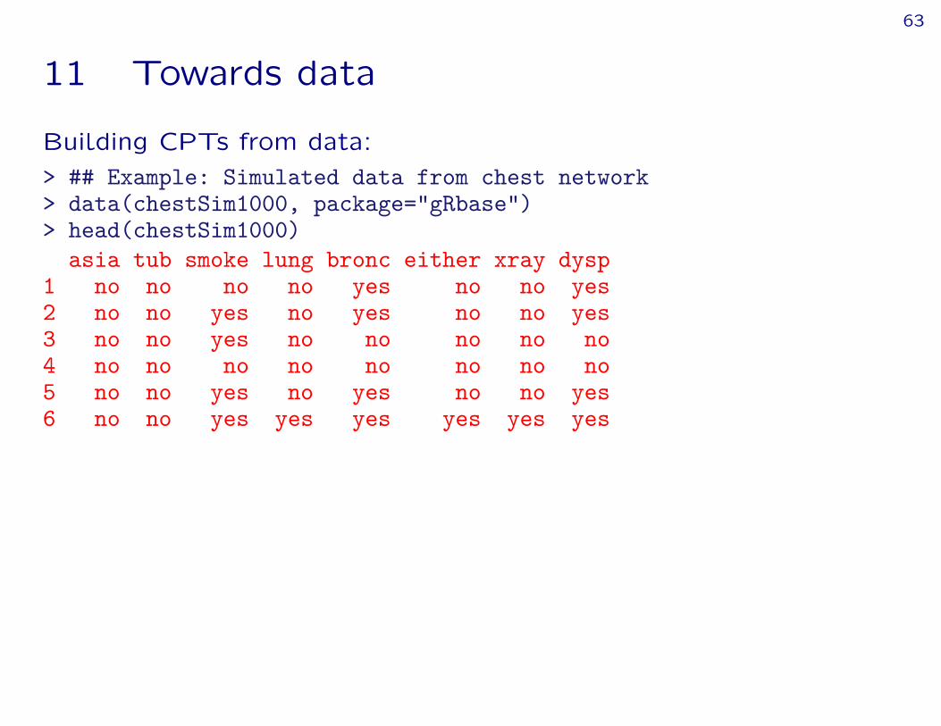
Building CPTs from data:> ## Example: Simulated data from chest network> data(chestSim1000, package="gRbase")> head(chestSim1000)

asia tub smoke lung bronc either xray dysp1 no no no no yes no no yes2 no no yes no yes no no yes3 no no yes no no no no no4 no no no no no no no no5 no no yes no yes no no yes6 no no yes yes yes yes yes yes

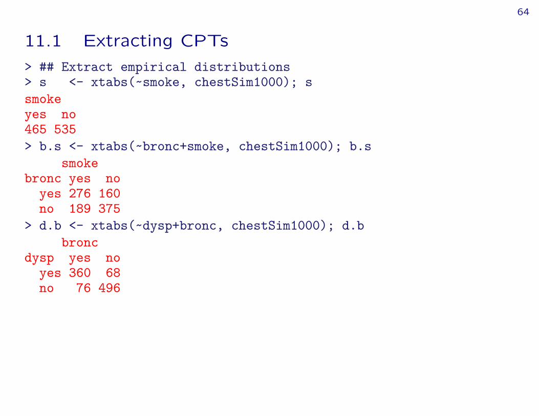
64

11.1 Extracting CPTs> ## Extract empirical distributions> s <- xtabs(~smoke, chestSim1000); ssmokeyes no465 535> b.s <- xtabs(~bronc+smoke, chestSim1000); b.s

smokebronc yes no

yes 276 160no 189 375

> d.b <- xtabs(~dysp+bronc, chestSim1000); d.bbronc

dysp yes noyes 360 68no 76 496

65

> ## Normalize to CPTs if desired (not necessary because> ## we can always normalize at the end)> s <- as.parray(s, normalize="first"); ssmoke

yes no0.465 0.535> b.s <- as.parray(b.s, normalize="first"); b.s

smokebronc yes no

yes 0.594 0.299no 0.406 0.701

> d.b <- as.parray(d.b, normalize="first"); d.bbronc

dysp yes noyes 0.826 0.121no 0.174 0.879

66

> cpt.list <- compileCPT(list(s, b.s, d.b)); cpt.listCPTspec with probabilities:P( smoke )P( bronc | smoke )P( dysp | bronc )

> net <- grain( cpt.list ); netIndependence network: Compiled: FALSE Propagated: FALSE

Nodes: chr [1:3] "smoke" "bronc" "dysp"

67

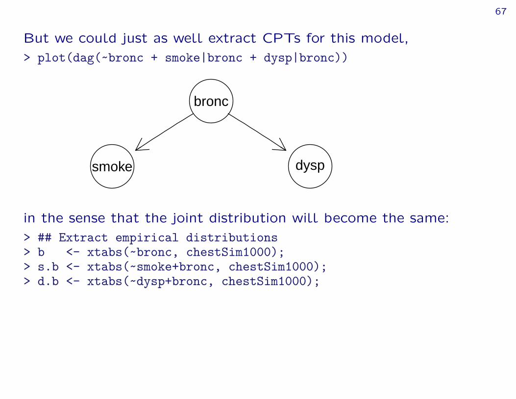
But we could just as well extract CPTs for this model,> plot(dag(~bronc + smoke|bronc + dysp|bronc))

bronc

smoke dysp

in the sense that the joint distribution will become the same:> ## Extract empirical distributions> b <- xtabs(~bronc, chestSim1000);> s.b <- xtabs(~smoke+bronc, chestSim1000);> d.b <- xtabs(~dysp+bronc, chestSim1000);

68

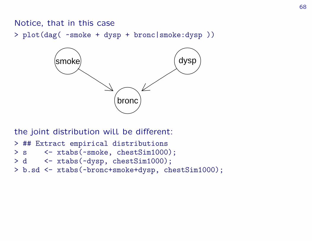
Notice, that in this case> plot(dag( ~smoke + dysp + bronc|smoke:dysp ))

smoke dysp

bronc

the joint distribution will be different:> ## Extract empirical distributions> s <- xtabs(~smoke, chestSim1000);> d <- xtabs(~dysp, chestSim1000);> b.sd <- xtabs(~bronc+smoke+dysp, chestSim1000);

69

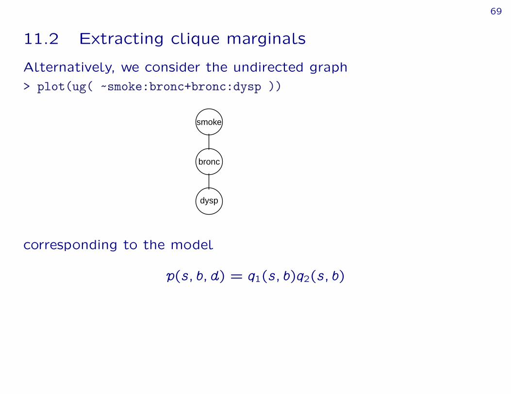
11.2 Extracting clique marginals

Alternatively, we consider the undirected graph> plot(ug( ~smoke:bronc+bronc:dysp ))

smoke

bronc

dysp

corresponding to the model

p(s; b; d) = q1(s; b)q2(s; b)

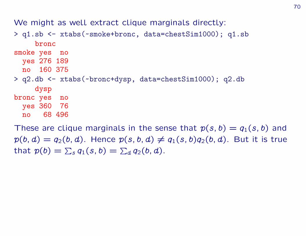
70

We might as well extract clique marginals directly:> q1.sb <- xtabs(~smoke+bronc, data=chestSim1000); q1.sb

broncsmoke yes no

yes 276 189no 160 375

> q2.db <- xtabs(~bronc+dysp, data=chestSim1000); q2.dbdysp

bronc yes noyes 360 76no 68 496

These are clique marginals in the sense that p(s; b) = q1(s; b) andp(b; d) = q2(b; d). Hence p(s; b; d) 6= q1(s; b)q2(b; d). But it is truethat p(b) =

Ps q1(s; b) =

Pd q2(b; d).

71

To obtain equality we must condition:

p(s; b; d) = p(sjb)p(b; d) = q1(s; b)

q1(b)q2(b; d)

so we set q1(s; b) q1(s; b)=q1(s):> q1.sb <- tableDiv(q1.sb, tableMargin(q1.sb, ~smoke)); q1.sb

broncsmoke yes no

yes 0.594 0.406no 0.299 0.701

Nowp(s; b; d) 6= q1(s; b)q2(b; d)

and the machinery for setting evidence etc. works as before.

72

12 Learning the model structure

The next step is to “learn” the structure of association between thevariables.

By this we mean learn the conditional independencies among thevariables from data.

Once we have this structure, we have seen how to turn thisstructure and data into a Bayesian network.

73

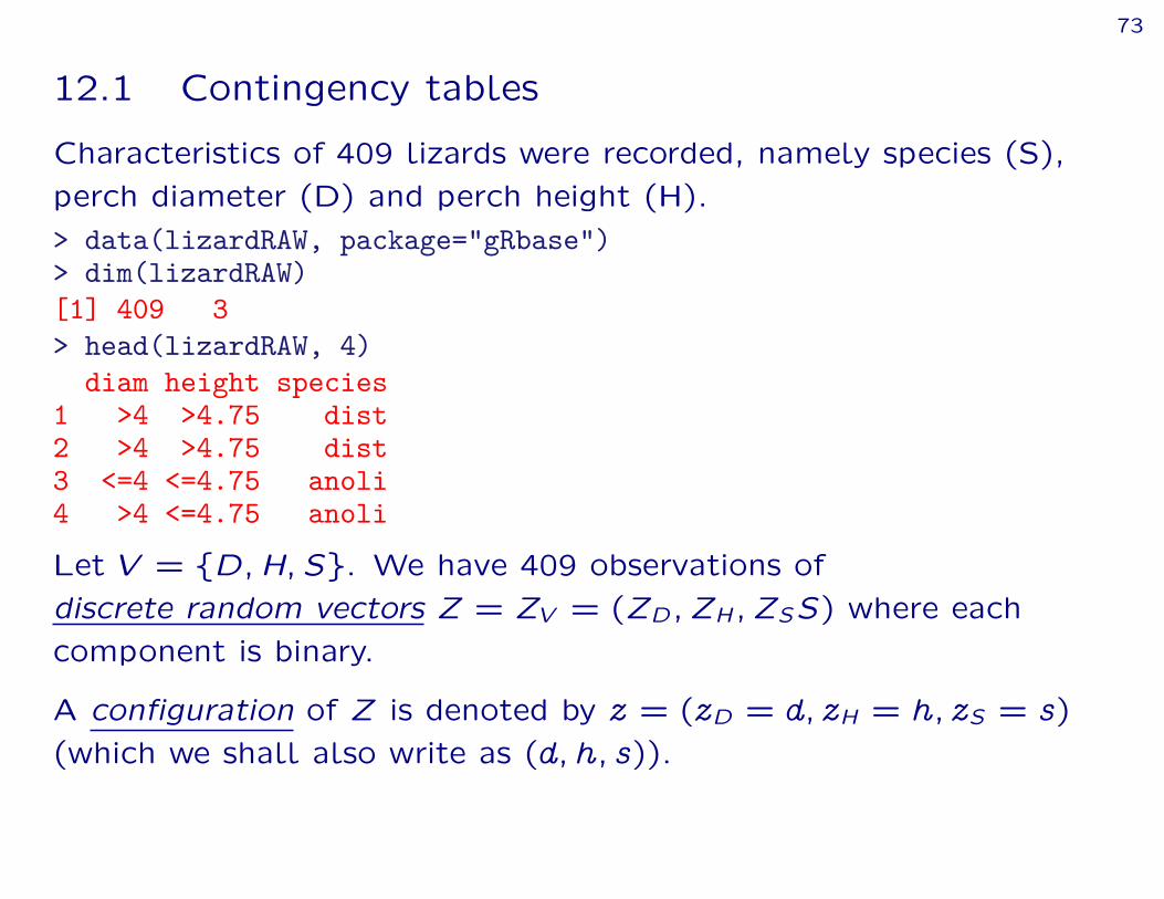
12.1 Contingency tables

Characteristics of 409 lizards were recorded, namely species (S),perch diameter (D) and perch height (H).> data(lizardRAW, package="gRbase")> dim(lizardRAW)[1] 409 3> head(lizardRAW, 4)

diam height species1 >4 >4.75 dist2 >4 >4.75 dist3 <=4 <=4.75 anoli4 >4 <=4.75 anoli

Let V = fD;H; Sg. We have 409 observations ofdiscrete random vectors Z = ZV = (ZD; ZH; ZSS) where eachcomponent is binary.

A configuration of Z is denoted by z = (zD = d; zH = h; zS = s)

(which we shall also write as (d; h; s)).

74

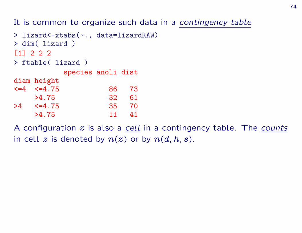
It is common to organize such data in a contingency table

> lizard<-xtabs(~., data=lizardRAW)> dim( lizard )[1] 2 2 2> ftable( lizard )

species anoli distdiam height<=4 <=4.75 86 73

>4.75 32 61>4 <=4.75 35 70

>4.75 11 41

A configuration z is also a cell in a contingency table. The countsin cell z is denoted by n(z) or by n(d; h; s).

75

The probability of a configuration z = (d; h; s) is denoted p(z) andthis is also the probability of a lizard falling in the (d; h; s) cell.

One estimate of the probabilities is by the relative frquencies:> lizardProb <- lizard/sum(lizard); ftable(lizardProb)

species anoli distdiam height<=4 <=4.75 0.2103 0.1785

>4.75 0.0782 0.1491>4 <=4.75 0.0856 0.1711

>4.75 0.0269 0.1002

76

For A V we have a marginal table with counts n(zA), forexample> tableMargin(lizard, ~height+species)

speciesheight anoli dist

<=4.75 121 143>4.75 43 102

The probability of an observation in a marginal cell zA isp(zA) =

Pz0:z0

A=zA p(z

0). For example

> tableMargin(lizardProb, ~height+species)species

height anoli dist<=4.75 0.296 0.350>4.75 0.105 0.249

77

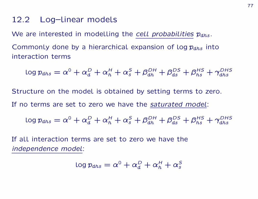
12.2 Log–linear models

We are interested in modelling the cell probabilities pdhs.

Commonly done by a hierarchical expansion of log pdhs intointeraction terms

log pdhs = ¸0 + ¸Dd + ¸Hh + ¸

Ss + ˛

DHdh + ˛

DSds + ˛

HShs + ‚

DHSdhs

Structure on the model is obtained by setting terms to zero.

If no terms are set to zero we have the saturated model:

log pdhs = ¸0 + ¸Dd + ¸Hh + ¸

Ss + ˛

DHdh + ˛

DSds + ˛

HShs + ‚

DHSdhs

If all interaction terms are set to zero we have theindependence model:

log pdhs = ¸0 + ¸Dd + ¸Hh + ¸

Ss

78

If an interaction term is set to zero then all higher order termscontaining that interaction terms must also be set to zero.

For example, if we set ˛DHdh = 0 then we must also set ‚DHSdhs = 0.

log pdhs = ¸0 + ¸Dd + ¸Hh + ¸

Ss + ˛

DSds + ˛

HShs +

The non–zero interaction terms are the generators of the model.Setting ˛DHdh = ‚DHSdhs = 0 the generators are

fD;H; S;DS;HSg

79

Generators contained in higher order generators can be omitted sothe generators become

fDS;HSg

corresponding tolog pdhs = ¸DSds + ¸

HShs

Because of this log–linear expansions, the models are calledlog–linear models.

Instead of taking logs we may write phds in product form

pdhs = qDS(d; s)qHS(h; s)

and this is in some connections useful.

For example, the factorization criterion gives directly thatD??H jS.

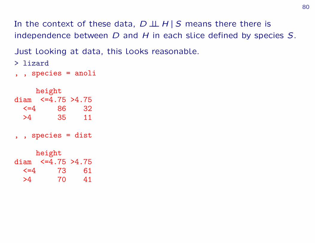
80

In the context of these data, D??H jS means there there isindependence between D and H in each slice defined by species S.

Just looking at data, this looks reasonable.> lizard, , species = anoli

heightdiam <=4.75 >4.75

<=4 86 32>4 35 11

, , species = dist

heightdiam <=4.75 >4.75

<=4 73 61>4 70 41

81

12.3 Hierarchical log–linear models

More generally the generating class of a log–linear model is a setA = fA1; : : : ; AQg where Aq V .

This corresponds top(z) =

YA2A

qA(zA)

where qA is a potential, a function that depends on z only throughzA.

82

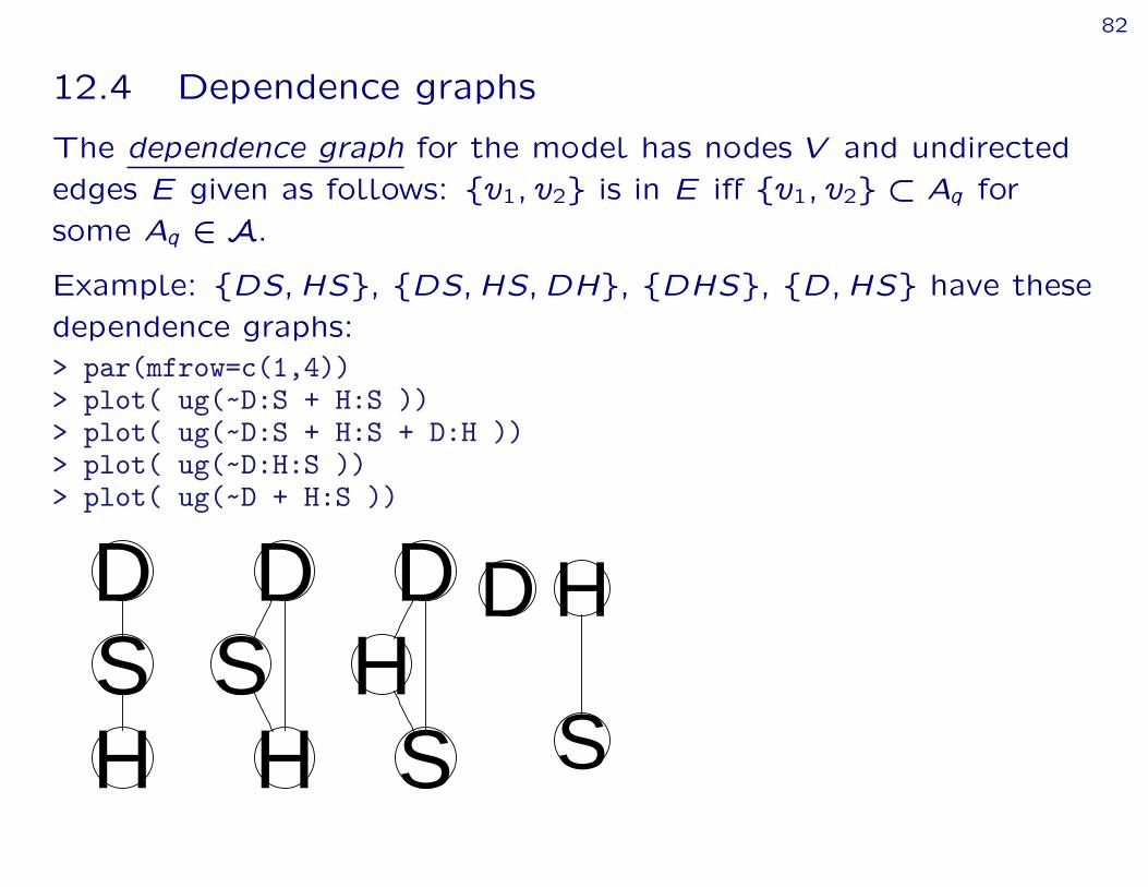
12.4 Dependence graphs

The dependence graph for the model has nodes V and undirectededges E given as follows: fv1; v2g is in E iff fv1; v2g Aq forsome Aq 2 A.

Example: fDS;HSg, fDS;HS;DHg, fDHSg, fD;HSg have thesedependence graphs:> par(mfrow=c(1,4))> plot( ug(~D:S + H:S ))> plot( ug(~D:S + H:S + D:H ))> plot( ug(~D:H:S ))> plot( ug(~D + H:S ))

DSH

DSH

DHS

D H

S

83

12.5 The Global Markov property

There is a general rule reading conditional independencies from agraph: If two sets of nodes U and V are separated by a third set Wthen U?? V jW .

Example: fE; Fg??AjfB;Cg.> plot( ug(~A:B:C+B:C:D+D:E+E:F ))

A

B

C

D

E

F

84

12.6 Estimation – likelihood equations

Under multinomial sampling the likelihood is

L =Y

all states z

p(z)n(z) =YA2A

YzA

qA(zA)n(zA)

The MLE p̂(z) for p(z) is the (unique) solution to the likelihoodequations

p̂(zA) = n(zA)=n; A 2 A

Typically MLE must be found by iterative methods, e.g. iterativeproportional scaling (IPS).

However, for some log–linear models (called decomposablemodels) the MLE can be found in closed form. In this case IPSconverges in 2 iterations.

85

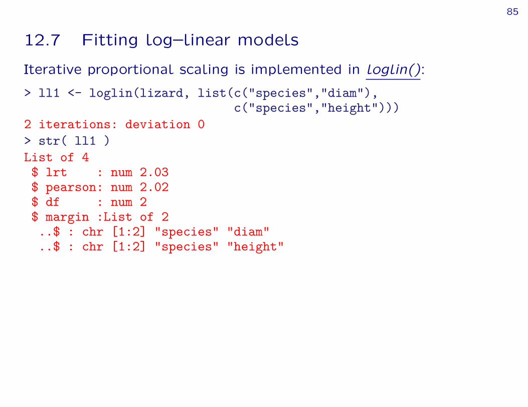
12.7 Fitting log–linear models

Iterative proportional scaling is implemented in loglin():

> ll1 <- loglin(lizard, list(c("species","diam"),c("species","height")))

2 iterations: deviation 0> str( ll1 )List of 4$ lrt : num 2.03$ pearson: num 2.02$ df : num 2$ margin :List of 2..$ : chr [1:2] "species" "diam"..$ : chr [1:2] "species" "height"

86

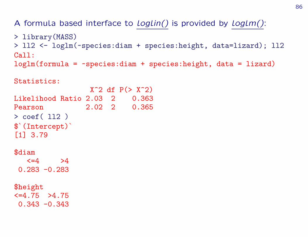
A formula based interface to loglin() is provided by loglm():

> library(MASS)> ll2 <- loglm(~species:diam + species:height, data=lizard); ll2Call:loglm(formula = ~species:diam + species:height, data = lizard)

Statistics:X^2 df P(> X^2)

Likelihood Ratio 2.03 2 0.363Pearson 2.02 2 0.365> coef( ll2 )$`(Intercept)`[1] 3.79

$diam<=4 >4

0.283 -0.283

$height<=4.75 >4.750.343 -0.343

87

$speciesanoli dist

-0.309 0.309

$diam.speciesspecies

diam anoli dist<=4 0.188 -0.188>4 -0.188 0.188

$height.speciesspecies

height anoli dist<=4.75 0.174 -0.174>4.75 -0.174 0.174

88

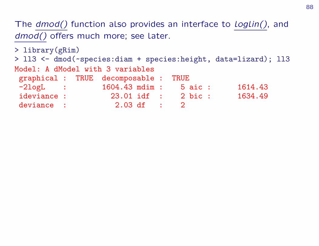
The dmod() function also provides an interface to loglin(), anddmod() offers much more; see later.

> library(gRim)> ll3 <- dmod(~species:diam + species:height, data=lizard); ll3Model: A dModel with 3 variablesgraphical : TRUE decomposable : TRUE-2logL : 1604.43 mdim : 5 aic : 1614.43ideviance : 23.01 idf : 2 bic : 1634.49deviance : 2.03 df : 2

89

12.8 Graphical models and decomposable models

Let Z = (Zv; v 2 V ) be a random vector and letA = fA1; : : : ; AQg where Aq V be a generating class for a loglinear model corresponding to

p(z) =YA2A

qA(zA)

90

Definition 1 A hierarchical log–linear model with generating classA = fa1; : : : aQg is graphical if A are the cliques of thedependence graph.

> par(mfrow=c(1,4))> plot( ug(~D:S + H:S )) ## graphical> plot( ug(~D:S + H:S + D:H )) ## not graphical> plot( ug(~D:H:S )) ## graphical> plot( ug(~D + H:S )) ## graphical

DSH

DS

H

DH

S

D HS

91

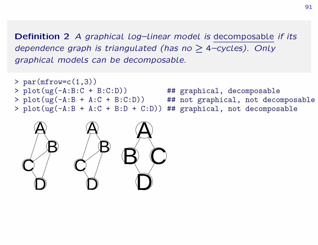
Definition 2 A graphical log–linear model is decomposable if itsdependence graph is triangulated (has no – 4–cycles). Onlygraphical models can be decomposable.

> par(mfrow=c(1,3))> plot(ug(~A:B:C + B:C:D)) ## graphical, decomposable> plot(ug(~A:B + A:C + B:C:D)) ## not graphical, not decomposable> plot(ug(~A:B + A:C + B:D + C:D)) ## graphical, not decomposable

AB

CD

AB

CD

AB C

D

92

12.9 ML estimation in decomposable models

Major point: ML estimates in decomposable models can be foundin closed form (no iterations). Consider lizard data:

The saturated model fDHSg (i.e. no restrictions on pdhs) isdecomposable, and the MLE is

p̂dhs = n(d; h; s)=n

Next consider the decomposable model fDS;HSg. The terminteraction DS can also be seen as the saturated model for themarginal table> n.ds <- tableMargin(lizard, ~diam+species); n.ds

speciesdiam anoli dist

<=4 118 134>4 46 111

i.e. there is no restriction on pds, and the MLE is p̂ds = n(d; s)=n.

93

Generally, for a decomposable model, the MLE can be found inclosed form as

p̂(z) =

QC:cliques p̂C(zC)Q

S:separators p̂S(zS)

where p̂E(zE) = n(zE)=n for any clique or separator E.

So for fDS;HSg we have

p̂dhs =p̂dsp̂hs

p̂s=[n(d; s)=n][n(h; s)=n]

n(s)=n

It is easy to see that we have the MLE: The MLE p̂dhs is thesolution to the equation

p̂ds = n(d; s)=n; p̂hs = n(h; s)=n

94

> n.ds <- tableMargin(lizard, c("diam", "species"))> n.hs <- tableMargin(lizard, c("height", "species"))> n.s <- tableMargin(lizard, c("species"))> ec <- tableDiv( tableMult(n.ds, n.hs), n.s) ## expected counts> ftable( ec )

diam <=4 >4species heightanoli <=4.75 87.1 33.9

>4.75 30.9 12.1dist <=4.75 78.2 64.8

>4.75 55.8 46.2> ftable( fitted(ll2) )Re-fitting to get fitted values

species anoli distdiam height<=4 <=4.75 87.1 78.2

>4.75 30.9 55.8>4 <=4.75 33.9 64.8

>4.75 12.1 46.2

95

13 Decomposable models and Bayesiannetworks

Now is the time to establish connections between decomposablegraphical models and Bayesian networks.

› For a decomposable model, the MLE is given as

p̂(z) =

QC:cliques p̂C(zC)Q

S:separators p̂S(zS)=

QC:cliques n(zC)=nQ

S:separators n(zS)=n

› Major point: The above is IMPORTANT in connection withBayesian networks, it is a clique potential representation of p.

› Hence if we find a decomposable graphical model then we canconvert this to a Bayesian network.

› We need not specify conditional probability tables (they areonly used for specifying the model anyway, the realcomputations takes place in the junction tree).

96

› There are 2Kn;2 graphical models with n variables, so modelsearch is a challenge. The number of decomposable models issmaller and these models can be fitted without iterations somodel search among decomposable models is faster.

97

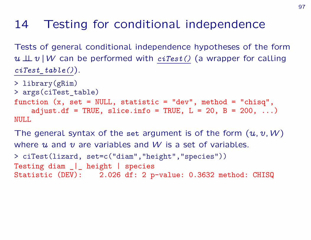
14 Testing for conditional independence

Tests of general conditional independence hypotheses of the formu?? v jW can be performed with ciTest() (a wrapper for callingciTest_table()).

> library(gRim)> args(ciTest_table)function (x, set = NULL, statistic = "dev", method = "chisq",

adjust.df = TRUE, slice.info = TRUE, L = 20, B = 200, ...)NULL

The general syntax of the set argument is of the form (u; v;W )where u and v are variables and W is a set of variables.> ciTest(lizard, set=c("diam","height","species"))Testing diam _|_ height | speciesStatistic (DEV): 2.026 df: 2 p-value: 0.3632 method: CHISQ

98

14.1 What is a CI-test – stratification

Conditional independence of u and v given W means independenceof u and v for each configuration w˜ of W .

In model terms, the test performed by ciTest() corresponds to thetest for removing the edge fu; vg from the saturated model withvariables fu; vg [W .

Conceptually form a factor S by crossing the factors in W . Thetest can then be formulated as a test of the conditionalindependence u?? v jS in a three way table.

The deviance decomposes into independent contributions from eachstratum:

D = 2Xijs

nijs lognijs

m̂ijs

=Xs

2Xij

nijs lognijs

m̂ijs

=Xs

Ds

where the contribution Ds from the sth slice is the deviance for theindependence model of u and v in that slice.

99

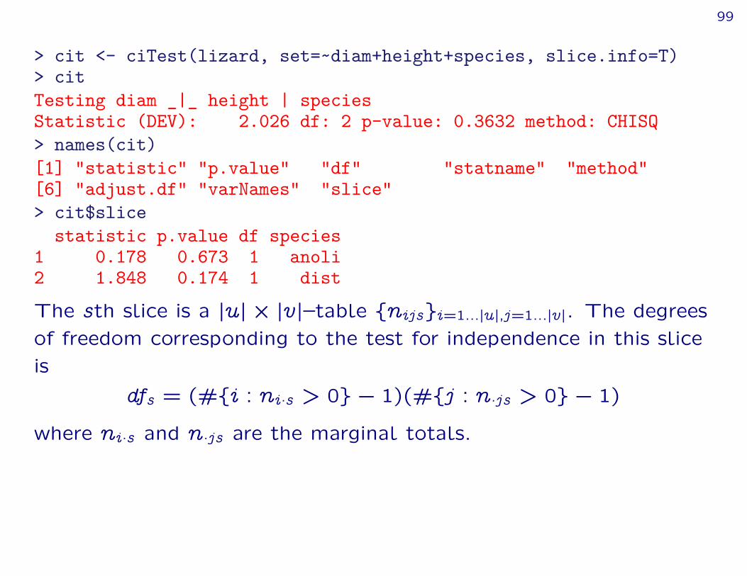
> cit <- ciTest(lizard, set=~diam+height+species, slice.info=T)> citTesting diam _|_ height | speciesStatistic (DEV): 2.026 df: 2 p-value: 0.3632 method: CHISQ> names(cit)[1] "statistic" "p.value" "df" "statname" "method"[6] "adjust.df" "varNames" "slice"> cit$slice

statistic p.value df species1 0.178 0.673 1 anoli2 1.848 0.174 1 dist

The sth slice is a juj ˆ jvj–table fnijsgi=1:::juj;j=1:::jvj. The degreesof freedom corresponding to the test for independence in this sliceis

dfs = (#fi : ni´s > 0g ` 1)(#fj : n´js > 0g ` 1)

where ni´s and n´js are the marginal totals.

100

14.2 Example: University admissions

Example: Admission to graduate school at UC at Berkley in 1973for the six largest departments classified by sex and gender.> ftable(UCBAdmissions)

Dept A B C D E FAdmit GenderAdmitted Male 512 353 120 138 53 22

Female 89 17 202 131 94 24Rejected Male 313 207 205 279 138 351

Female 19 8 391 244 299 317

Is there evidence of sexual discrimination?> ag <- tableMargin(UCBAdmissions, ~Admit+Gender); ag

GenderAdmit Male Female

Admitted 1198 557Rejected 1493 1278

> as.parray( ag, normalize="first" )Gender

Admit Male FemaleAdmitted 0.445 0.304Rejected 0.555 0.696

101

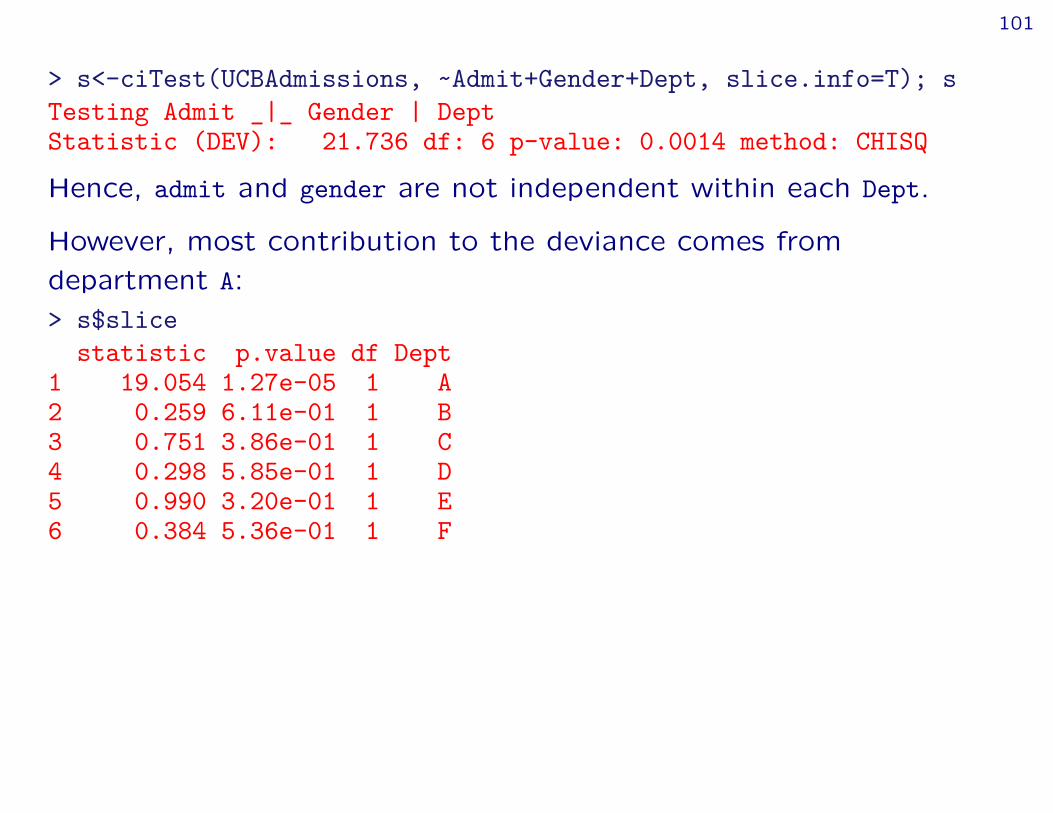
> s<-ciTest(UCBAdmissions, ~Admit+Gender+Dept, slice.info=T); sTesting Admit _|_ Gender | DeptStatistic (DEV): 21.736 df: 6 p-value: 0.0014 method: CHISQ

Hence, admit and gender are not independent within each Dept.

However, most contribution to the deviance comes fromdepartment A:> s$slice

statistic p.value df Dept1 19.054 1.27e-05 1 A2 0.259 6.11e-01 1 B3 0.751 3.86e-01 1 C4 0.298 5.85e-01 1 D5 0.990 3.20e-01 1 E6 0.384 5.36e-01 1 F

102

So what happens in department A?> x <- tableSlice(UCBAdmissions, margin="Dept", level="A"); x

GenderAdmit Male Female

Admitted 512 89Rejected 313 19

> as.parray(x, normalize="first")Gender

Admit Male FemaleAdmitted 0.621 0.824Rejected 0.379 0.176

The discrimination is against men!

103

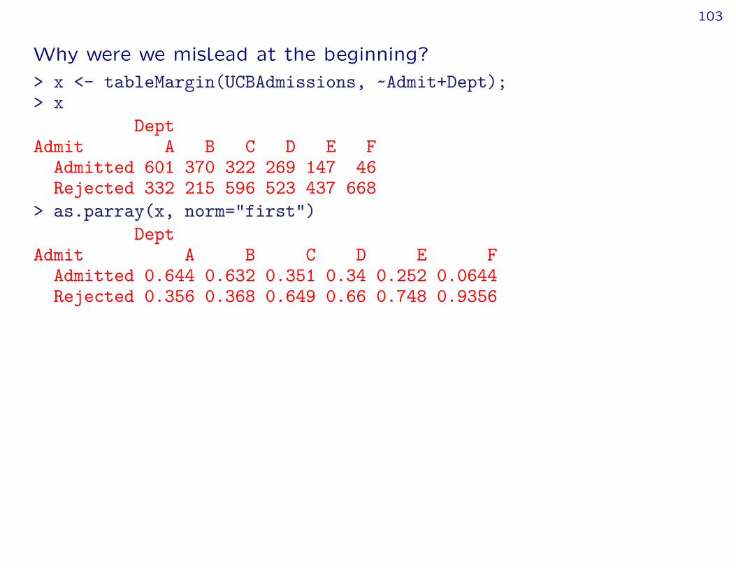
Why were we mislead at the beginning?> x <- tableMargin(UCBAdmissions, ~Admit+Dept);> x

DeptAdmit A B C D E F

Admitted 601 370 322 269 147 46Rejected 332 215 596 523 437 668

> as.parray(x, norm="first")Dept

Admit A B C D E FAdmitted 0.644 0.632 0.351 0.34 0.252 0.0644Rejected 0.356 0.368 0.649 0.66 0.748 0.9356

104

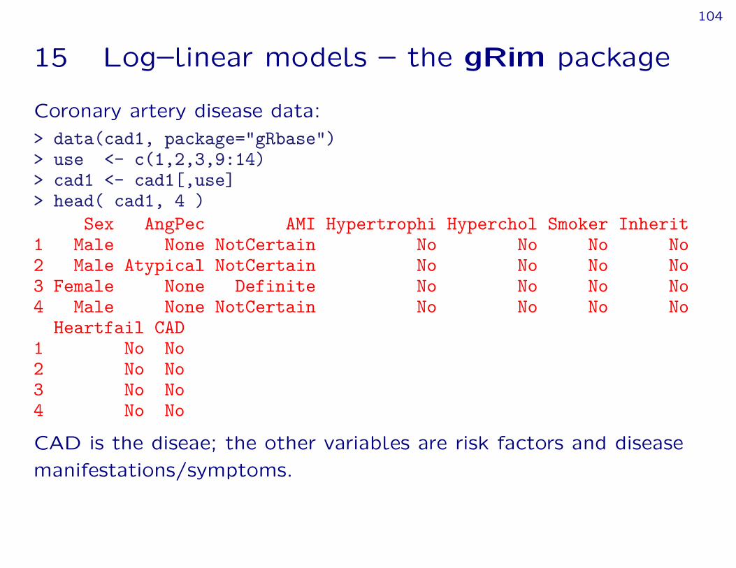
15 Log–linear models – the gRim package

Coronary artery disease data:> data(cad1, package="gRbase")> use <- c(1,2,3,9:14)> cad1 <- cad1[,use]> head( cad1, 4 )

Sex AngPec AMI Hypertrophi Hyperchol Smoker Inherit1 Male None NotCertain No No No No2 Male Atypical NotCertain No No No No3 Female None Definite No No No No4 Male None NotCertain No No No No

Heartfail CAD1 No No2 No No3 No No4 No No

CAD is the diseae; the other variables are risk factors and diseasemanifestations/symptoms.

105

Some (random) model:> m1 <- dmod(~Sex:Smoker:CAD + CAD:Hyperchol:AMI, data=cad1); m1Model: A dModel with 5 variablesgraphical : TRUE decomposable : TRUE-2logL : 1293.88 mdim : 13 aic : 1319.88ideviance : 112.54 idf : 8 bic : 1364.91deviance : 16.38 df : 18

> plot( m1 )

Sex

Smoker

CAD

Hyperchol

AMI

106

› Data must be a table or a dataframe (which will be convertedto a table).

› Variable names may be abbreviated.

› Instead of a formula, a list can be given.

› The generating class as a list is retrieved with terms() and as aformula with formula():> str( terms( m1 ) )List of 2$ : chr [1:3] "Sex" "Smoker" "CAD"$ : chr [1:3] "CAD" "Hyperchol" "AMI"

> formula( m1 )~Sex * Smoker * CAD + CAD * Hyperchol * AMI

107

Notice: No dependence graph in model object; must be generatedon the fly using ugList():

> # Default: a graphNEL object> DG <- ugList( terms( m1 ) ); DGA graphNEL graph with undirected edgesNumber of Nodes = 5Number of Edges = 6> # Alternative: an adjacency matrix> a <- ugList( terms( m1 ), result="matrix" ); a

Sex Smoker CAD Hyperchol AMISex 0 1 1 0 0Smoker 1 0 1 0 0CAD 1 1 0 1 1Hyperchol 0 0 1 0 1AMI 0 0 1 1 0> A <- ugList( terms( m1 ), result="dgCMatrix" )

108

15.1 Model specification shortcuts

Shortcuts for specifying some models> mar <- c("Sex","AngPec","AMI","CAD")> str(terms(dmod(~.^., data=cad1, margin=mar))) ## Saturated modelList of 1$ : chr [1:4] "Sex" "AngPec" "AMI" "CAD"

> str(terms(dmod(~.^1, data=cad1, margin=mar))) ## Independence modelList of 4$ : chr "Sex"$ : chr "AngPec"$ : chr "AMI"$ : chr "CAD"

> str(terms(dmod(~.^3, data=cad1, margin=mar))) ## All 3-factor modelList of 4$ : chr [1:3] "Sex" "AngPec" "AMI"$ : chr [1:3] "Sex" "AngPec" "CAD"$ : chr [1:3] "Sex" "AMI" "CAD"$ : chr [1:3] "AngPec" "AMI" "CAD"

109

15.2 Altering graphical models

Natural operations on graphical models: add and delete edges> m1 <- dmod(~Sex:Smoker:CAD + CAD:Hyperchol:AMI, data=cad1); m1Model: A dModel with 5 variablesgraphical : TRUE decomposable : TRUE-2logL : 1293.88 mdim : 13 aic : 1319.88ideviance : 112.54 idf : 8 bic : 1364.91deviance : 16.38 df : 18

> m2 <- update(m1,items =list(dedge=~Hyperchol:CAD, # drop edge

aedge=~Smoker:AMI)) # add edge> par(mfrow=c(1,2)); plot( m1 ); plot( m2 )

110

Sex

Smoker

CAD

Hyperchol

AMI

Sex

Smoker

CAD Hyperchol

AMI

111

15.3 Model comparison

Models are compared with compareModels().

> m1 <- dmod(~Sex:Smoker:CAD + CAD:Hyperchol:AMI, data=cad1); m1Model: A dModel with 5 variablesgraphical : TRUE decomposable : TRUE-2logL : 1293.88 mdim : 13 aic : 1319.88ideviance : 112.54 idf : 8 bic : 1364.91deviance : 16.38 df : 18

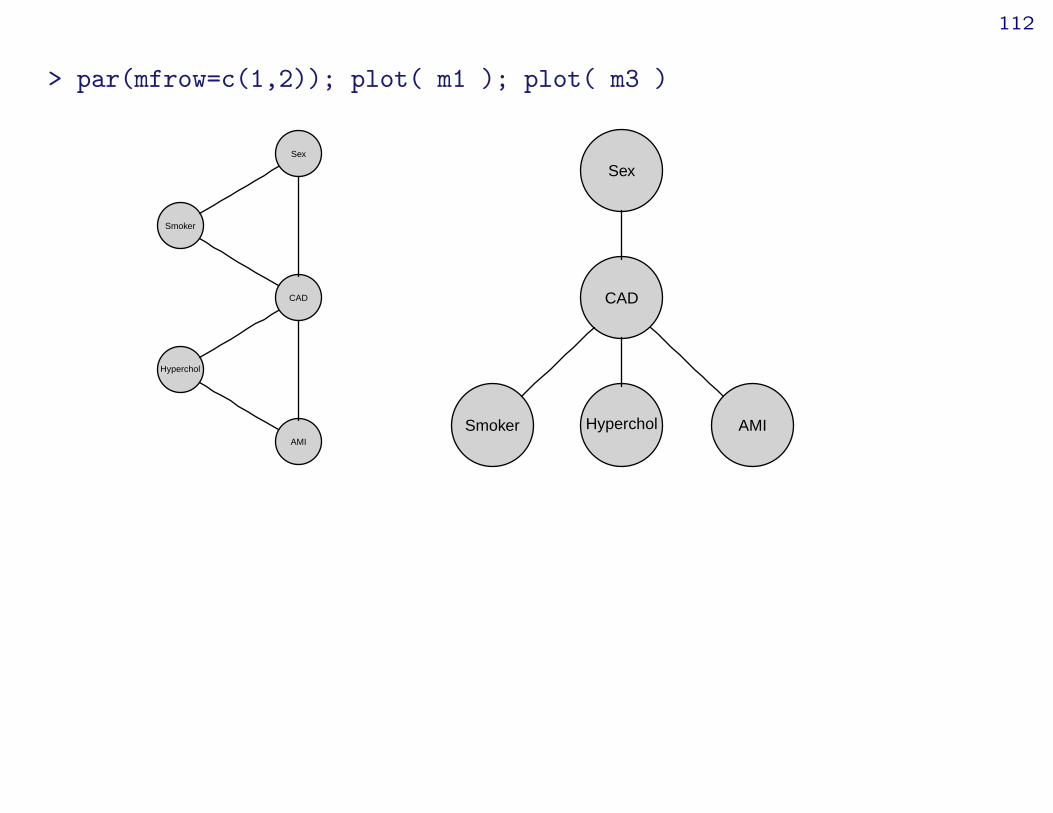
> m3 <- update(m1, items=list(dedge=~Sex:Smoker+Hyperchol:AMI))> compareModels( m1, m3 )Large:

:"Sex" "Smoker" "CAD":"CAD" "Hyperchol" "AMI"

Small::"Sex" "CAD":"Smoker" "CAD":"CAD" "Hyperchol":"CAD" "AMI"

-2logL: 8.93 df: 4 AIC(k= 2.0): 0.93 p.value: 0.346446

112

> par(mfrow=c(1,2)); plot( m1 ); plot( m3 )

Sex

Smoker

CAD

Hyperchol

AMI

Sex

CAD

Smoker Hyperchol AMI

113

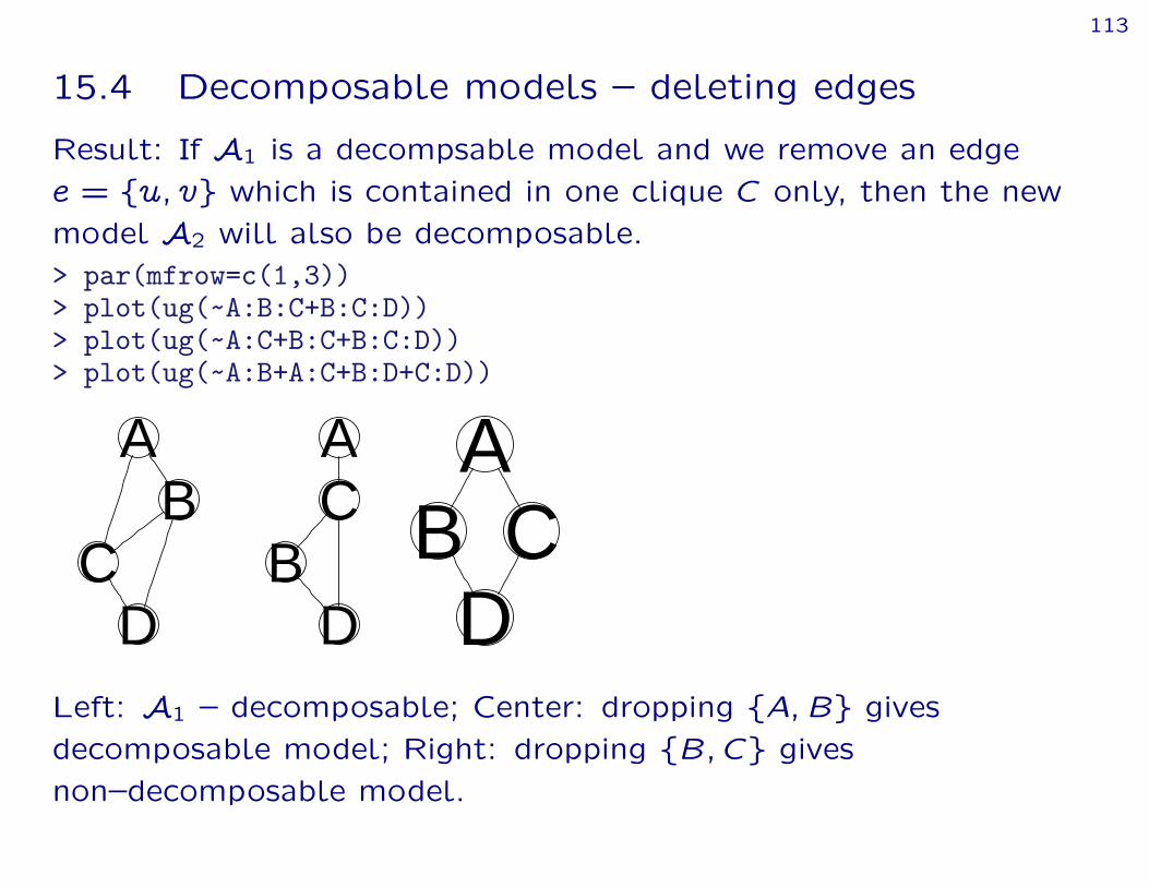
15.4 Decomposable models – deleting edges

Result: If A1 is a decompsable model and we remove an edgee = fu; vg which is contained in one clique C only, then the newmodel A2 will also be decomposable.> par(mfrow=c(1,3))> plot(ug(~A:B:C+B:C:D))> plot(ug(~A:C+B:C+B:C:D))> plot(ug(~A:B+A:C+B:D+C:D))

AB

CD

AC

BD

AB C

DLeft: A1 – decomposable; Center: dropping fA;Bg givesdecomposable model; Right: dropping fB;Cg givesnon–decomposable model.

114

Result: The test for removal of e = fu; vg which is contained inone clique C only can be made as a test for u?? vjC n fu; vg inthe C–marginal table.

This is done by ciTest(). Hence, no model fitting is necessary.

115

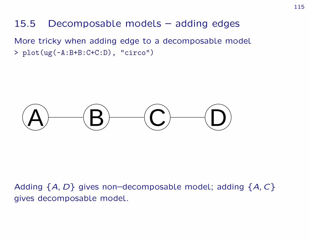
15.5 Decomposable models – adding edges

More tricky when adding edge to a decomposable model> plot(ug(~A:B+B:C+C:D), "circo")

A B C D

Adding fA;Dg gives non–decomposable model; adding fA; Cggives decomposable model.

116

One solution: Try adding edge to graph and test if new graph isdecomposable. Can be tested with maximum cardinality search asimplemented in mcs(). Runs in O(jedgesj+ jverticesj).> UG <- ug(~A:B+B:C+C:D)> mcs(UG)[1] "A" "B" "C" "D"> UG1 <- addEdge("A","D",UG)> mcs(UG1)character(0)> UG2 <- addEdge("A","C",UG)> mcs(UG2)[1] "A" "B" "C" "D"

117

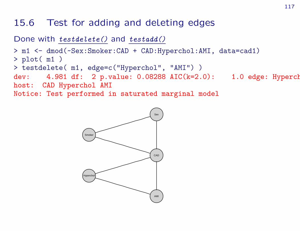
15.6 Test for adding and deleting edges

Done with testdelete() and testadd()> m1 <- dmod(~Sex:Smoker:CAD + CAD:Hyperchol:AMI, data=cad1)> plot( m1 )> testdelete( m1, edge=c("Hyperchol", "AMI") )dev: 4.981 df: 2 p.value: 0.08288 AIC(k=2.0): 1.0 edge: Hyperchol:AMIhost: CAD Hyperchol AMINotice: Test performed in saturated marginal model

Sex

Smoker

CAD

Hyperchol

AMI

118

> m1 <- dmod(~Sex:Smoker:CAD + CAD:Hyperchol:AMI, data=cad1)> plot( m1 )> testadd( m1, edge=c("Smoker", "Hyperchol"))dev: 1.658 df: 2 p.value: 0.43654 AIC(k=2.0): 2.3 edge: Smoker:Hypercholhost: CAD Smoker HypercholNotice: Test performed in saturated marginal model

Sex

Smoker

CAD

Hyperchol

AMI

119

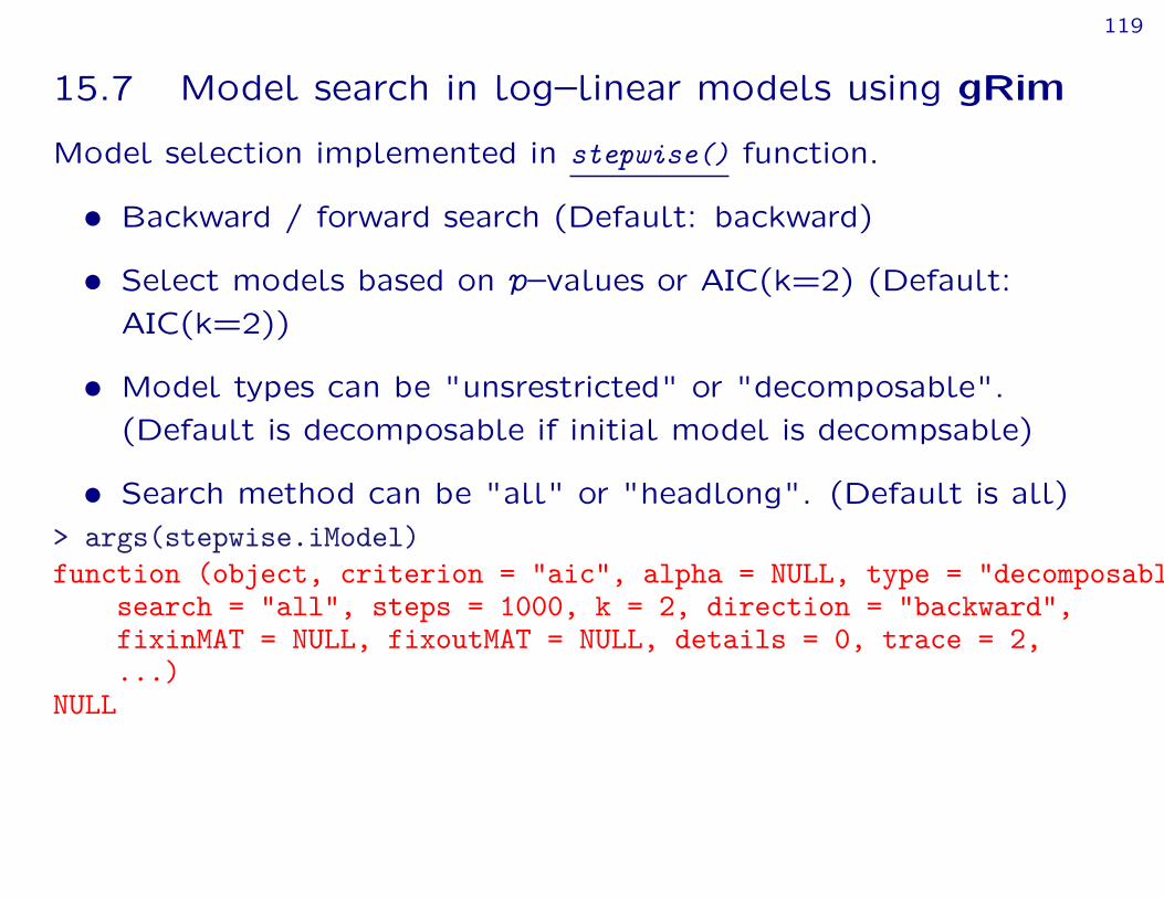
15.7 Model search in log–linear models using gRim

Model selection implemented in stepwise() function.

› Backward / forward search (Default: backward)

› Select models based on p–values or AIC(k=2) (Default:AIC(k=2))

› Model types can be "unsrestricted" or "decomposable".(Default is decomposable if initial model is decompsable)

› Search method can be "all" or "headlong". (Default is all)> args(stepwise.iModel)function (object, criterion = "aic", alpha = NULL, type = "decomposable",

search = "all", steps = 1000, k = 2, direction = "backward",fixinMAT = NULL, fixoutMAT = NULL, details = 0, trace = 2,...)

NULL

120

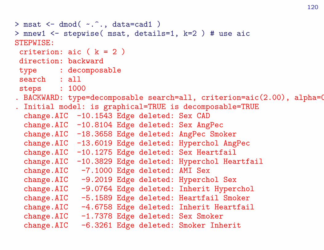
> msat <- dmod( ~.^., data=cad1 )> mnew1 <- stepwise( msat, details=1, k=2 ) # use aicSTEPWISE:criterion: aic ( k = 2 )direction: backwardtype : decomposablesearch : allsteps : 1000

. BACKWARD: type=decomposable search=all, criterion=aic(2.00), alpha=0.00

. Initial model: is graphical=TRUE is decomposable=TRUEchange.AIC -10.1543 Edge deleted: Sex CADchange.AIC -10.8104 Edge deleted: Sex AngPecchange.AIC -18.3658 Edge deleted: AngPec Smokerchange.AIC -13.6019 Edge deleted: Hyperchol AngPecchange.AIC -10.1275 Edge deleted: Sex Heartfailchange.AIC -10.3829 Edge deleted: Hyperchol Heartfailchange.AIC -7.1000 Edge deleted: AMI Sexchange.AIC -9.2019 Edge deleted: Hyperchol Sexchange.AIC -9.0764 Edge deleted: Inherit Hypercholchange.AIC -5.1589 Edge deleted: Heartfail Smokerchange.AIC -4.6758 Edge deleted: Inherit Heartfailchange.AIC -1.7378 Edge deleted: Sex Smokerchange.AIC -6.3261 Edge deleted: Smoker Inherit

121

change.AIC -6.2579 Edge deleted: CAD Inherit

122

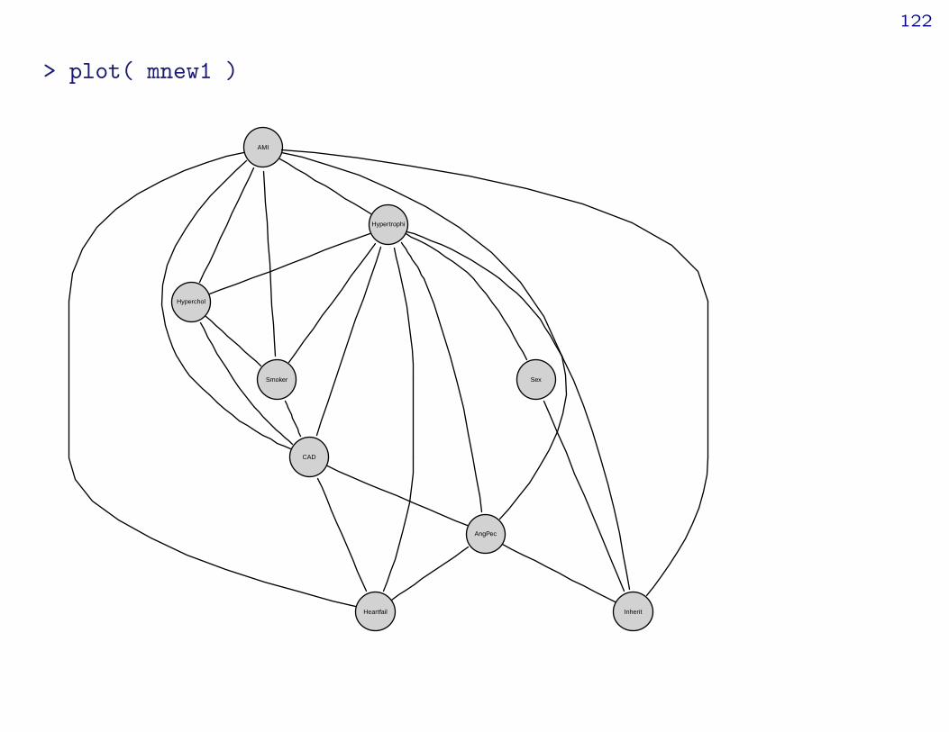
> plot( mnew1 )

AMI

Hypertrophi

Hyperchol

Smoker

CAD

AngPec

Heartfail

Sex

Inherit

123

> msat <- dmod( ~.^., data=cad1 )> mnew2 <- stepwise( msat, details=1, k=log(nrow(cad1)) ) # use bicSTEPWISE:criterion: aic ( k = 5.46 )direction: backwardtype : decomposablesearch : allsteps : 1000

. BACKWARD: type=decomposable search=all, criterion=aic(5.46), alpha=0.00

. Initial model: is graphical=TRUE is decomposable=TRUEchange.AIC -100.0382 Edge deleted: Sex AngPecchange.AIC -103.1520 Edge deleted: Hyperchol AngPecchange.AIC -74.2967 Edge deleted: Smoker AngPecchange.AIC -67.8590 Edge deleted: Sex Hypercholchange.AIC -60.3907 Edge deleted: AngPec Hypertrophichange.AIC -51.9489 Edge deleted: Heartfail Hypercholchange.AIC -50.8580 Edge deleted: Sex CADchange.AIC -43.8873 Edge deleted: AngPec Heartfailchange.AIC -41.3702 Edge deleted: AMI Sexchange.AIC -43.6158 Edge deleted: AMI Heartfailchange.AIC -40.2509 Edge deleted: Hyperchol Inheritchange.AIC -26.3511 Edge deleted: AngPec AMIchange.AIC -31.4947 Edge deleted: Inherit AMI

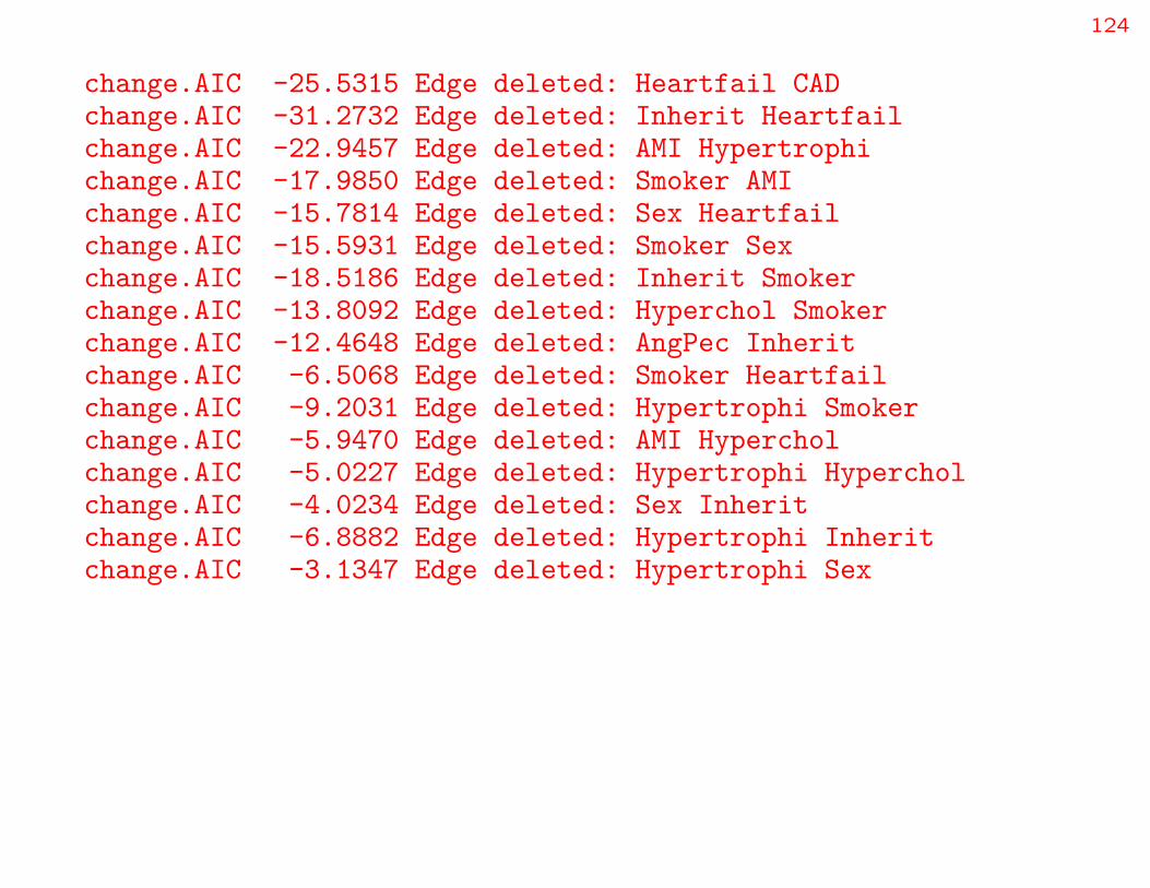
124

change.AIC -25.5315 Edge deleted: Heartfail CADchange.AIC -31.2732 Edge deleted: Inherit Heartfailchange.AIC -22.9457 Edge deleted: AMI Hypertrophichange.AIC -17.9850 Edge deleted: Smoker AMIchange.AIC -15.7814 Edge deleted: Sex Heartfailchange.AIC -15.5931 Edge deleted: Smoker Sexchange.AIC -18.5186 Edge deleted: Inherit Smokerchange.AIC -13.8092 Edge deleted: Hyperchol Smokerchange.AIC -12.4648 Edge deleted: AngPec Inheritchange.AIC -6.5068 Edge deleted: Smoker Heartfailchange.AIC -9.2031 Edge deleted: Hypertrophi Smokerchange.AIC -5.9470 Edge deleted: AMI Hypercholchange.AIC -5.0227 Edge deleted: Hypertrophi Hypercholchange.AIC -4.0234 Edge deleted: Sex Inheritchange.AIC -6.8882 Edge deleted: Hypertrophi Inheritchange.AIC -3.1347 Edge deleted: Hypertrophi Sex

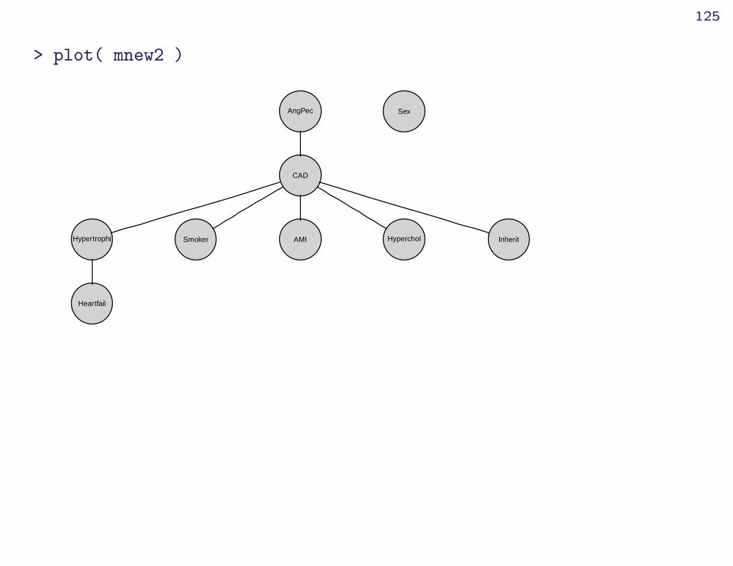
125

> plot( mnew2 )

AngPec

CAD

Hypertrophi

Heartfail

Smoker AMI Hyperchol Inherit

Sex

126

16 From graph and data to network

Create graphs from models:> ug1 <- ugList( terms( mnew1 ) )> ug2 <- ugList( terms( mnew2 ) )> par(mfrow=c(1,2)); plot( ug1 ); plot( ug2 )

●AMI

●Hypertrophi

●Hyperchol

●Smoker

●CAD

●AngPec

●Heartfail

●Sex

●Inherit

AngPec

CAD

Hypertrophi

Heartfail

Smoker AMI Hyperchol Inherit

Sex

127

Create Bayesian networks from (graph, data):> bn1 <- compile( grain( ug1, data=cad1, smooth=0.1 )); bn1Independence network: Compiled: TRUE Propagated: FALSE

Nodes: chr [1:9] "Hypertrophi" "AMI" "CAD" "Smoker" ...> bn2 <- compile( grain( ug2, data=cad1, smooth=0.1 )); bn2Independence network: Compiled: TRUE Propagated: FALSE

Nodes: chr [1:9] "CAD" "AngPec" "Hypertrophi" "Heartfail" ...

128

> querygrain( bn1, "CAD")$CADCAD

No Yes0.546 0.454> z<-setEvidence( bn1, nodes=c("AngPec", "Hypertrophi"),

c("Typical","Yes"))> # alternative form> z<-setEvidence( bn1,

nslist=list(AngPec="Typical", Hypertrophi="Yes"))> querygrain( z, "CAD")$CADCAD

No Yes0.599 0.401

129

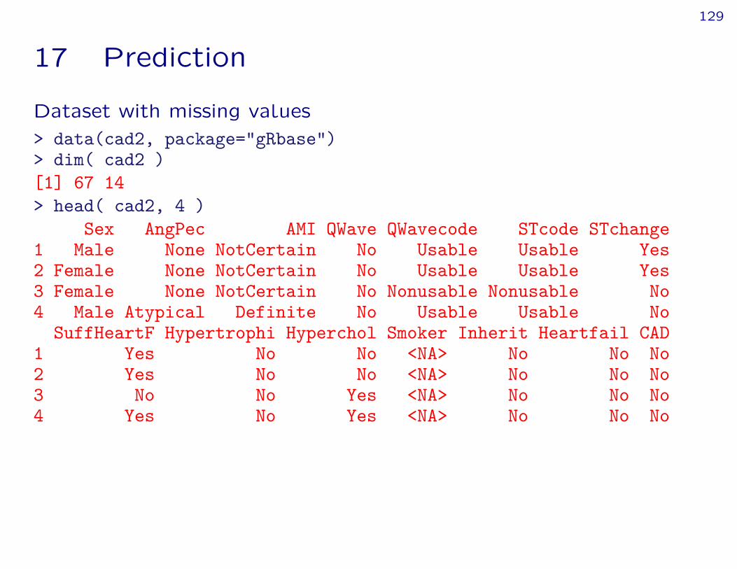
17 Prediction

Dataset with missing values> data(cad2, package="gRbase")> dim( cad2 )[1] 67 14> head( cad2, 4 )

Sex AngPec AMI QWave QWavecode STcode STchange1 Male None NotCertain No Usable Usable Yes2 Female None NotCertain No Usable Usable Yes3 Female None NotCertain No Nonusable Nonusable No4 Male Atypical Definite No Usable Usable No

SuffHeartF Hypertrophi Hyperchol Smoker Inherit Heartfail CAD1 Yes No No <NA> No No No2 Yes No No <NA> No No No3 No No Yes <NA> No No No4 Yes No Yes <NA> No No No

130

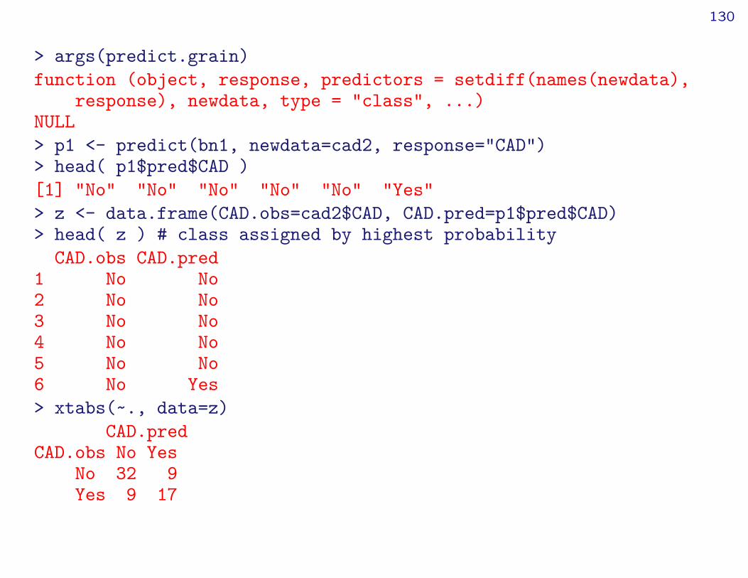
> args(predict.grain)function (object, response, predictors = setdiff(names(newdata),

response), newdata, type = "class", ...)NULL> p1 <- predict(bn1, newdata=cad2, response="CAD")> head( p1$pred$CAD )[1] "No" "No" "No" "No" "No" "Yes"> z <- data.frame(CAD.obs=cad2$CAD, CAD.pred=p1$pred$CAD)> head( z ) # class assigned by highest probability

CAD.obs CAD.pred1 No No2 No No3 No No4 No No5 No No6 No Yes> xtabs(~., data=z)

CAD.predCAD.obs No Yes

No 32 9Yes 9 17

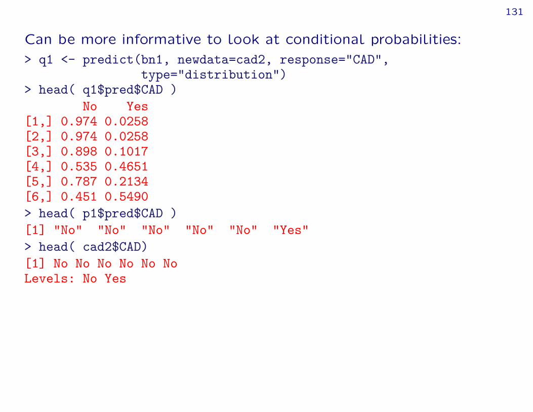
131

Can be more informative to look at conditional probabilities:> q1 <- predict(bn1, newdata=cad2, response="CAD",

type="distribution")> head( q1$pred$CAD )

No Yes[1,] 0.974 0.0258[2,] 0.974 0.0258[3,] 0.898 0.1017[4,] 0.535 0.4651[5,] 0.787 0.2134[6,] 0.451 0.5490> head( p1$pred$CAD )[1] "No" "No" "No" "No" "No" "Yes"> head( cad2$CAD)[1] No No No No No NoLevels: No Yes

132

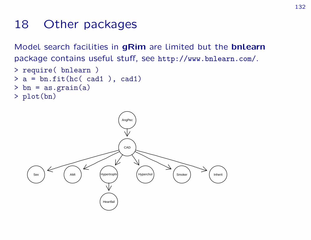
18 Other packages

Model search facilities in gRim are limited but the bnlearnpackage contains useful stuff, see http://www.bnlearn.com/.> require( bnlearn )> a = bn.fit(hc( cad1 ), cad1)> bn = as.grain(a)> plot(bn)

Sex

CAD

AngPec

AMI Hypertrophi Hyperchol Smoker Inherit

Heartfail

133

19 Winding up

Brief summary:

› We have gone through aspects of the gRain package and seensome of the mechanics of probability propagation.

› Propagation is based on factorization of a pmf according to adecomposable graph.

› We have gone through aspects of the gRim package and seenhow to search for decomposable graphical models.

› We have seen how to create a Bayesian network from thedependency graph of a decomposable graphical model.

› The model search facilities in gRim do not scale to largeproblems; instead it is more useful to consider other packagesfor structural learning, e.g. bnlearn.