grassland bird response to landscape-level and site
TRANSCRIPT
GRASSLAND BIRD RESPONSE TO LANDSCAPE-LEVEL AND SITE-SPECIFIC
VARIABLES IN THE LITTLE MISSOURI NATIONAL GRASSLAND
A Thesis Submitted to the Graduate Faculty
of the North Dakota State University
of Agriculture and Applied Science
By
Brian James Chepulis
In Partial Fulfillment of the Requirements for the Degree of
MASTER OF SCIENCE
Major Program: Natural Resources Management
April 2016
Fargo, North Dakota

North Dakota State University
Graduate School
Title GRASSLAND BIRD RESPONSE TO LANDSCAPE-LEVEL AND SITE-
SPECIFIC VARIABLES IN THE LITTLE MISSOURI NATIONAL GRASSLAND
By
Brian James Chepulis
The Supervisory Committee certifies that this disquisition complies with North Dakota
State University’s regulations and meets the accepted standards for the degree of
MASTER OF SCIENCE
SUPERVISORY COMMITTEE:
Edward Shawn DeKeyser
Chair
Lawrence D. Igl
Torre J. Hovick
Approved: 6 April 2016 Edward Shawn DeKeyser Date Department Chair

iii
ABSTRACT
Trend analysis from the North American Breeding Bird Survey indicates that the
Sprague’s pipit (Anthus spragueii) and Baird’s sparrow (Ammodramus bairdii) populations have
experienced severe annual declines of -3.5% and -3.0%, respectively, between 1966 and 2013.
The Little Missouri National Grassland (LMNG) in western North Dakota are listed as an
important breeding area for the Sprague’s pipit, Baird’s sparrow, and other grassland birds. Our
objectives for this study were to provide a better understanding of the effects of landscape-level
(e.g., oil development) and site-specific (e.g., vegetation structure) variables on sensitive
grassland bird populations in the LMNG. We surveyed 60 study sites twice each year (2014 and
2015) using a modified transect survey to evaluate grassland bird abundance. The results from
this study contributed to understanding grassland bird responses to landscape-level and site-
specific variables and identified specific mechanisms by which conservation measures for
declining grassland bird populations can be improved.

iv
ACKNOWLEDGMENTS
I would like to first thank the U.S Forest Service (USFS), Northern Prairie Wildlife
Research Center (NPWRC) of the U.S. Geological Survey (USGS, North Dakota EPSCoR
Graduate Research Assistantship program, and the Robert H. Levis II Cross Ranch Fellowship
for generously funding my research and graduate program. I thank NPWRC for providing a
travel trailer for my summer housing, and I extend a big thank you to Superintendent Valerie
Naylor and Administrative Technician Kevin Melzo of the National Park Service for assistance
in securing a safe place to park the trailer at the North Unit of Theodore Roosevelt National Park
(TRNP). Staff at the McKenzie Ranger District office of the USFS provided logistical
assistance. I especially would like to thank Kyle Dalzell of the McKenzie District office in
Watford City and Chadley Prosser of the Dakota Prairie Grasslands (DPG) office in Bismarck.
I owe a debt of gratitude to Larry Igl (USGS) and Dan Svingen (USFS) for securing
funding for this project when the initial funding fell through. None of this would have been
possible without their support. I appreciated all of the time, advice, and editing contributed by
my committee members, Drs. Larry Igl, Shawn DeKeyser, and Torre Hovick. Dr. Wesley
Newton (NPWRC) was extremely helpful with statistical advice and design. I also would like to
thank Betty Euliss (USGS) for her assistance with ArcMap during the early stages of study
design. Phil Sjursen (USFS) of the DPG office generously provided current GIS data layers for
the Little Missouri National Grassland.
I am appreciative to John Heiser (TRNP) for the advice and wisdom he provided on my
study area. Joe Orr assisted me in locating potential breeding areas for Sprague’s pipits in the
Little Missouri National Grassland in the summer of 2013. A big thank you goes to my
dedicated field assistants that worked on this project over the last two years: Joe Lamb, Brandon

v
Kaiser, Mason Ryckman, and Chris Sharpe. I would especially like to thank Brandon Kaiser and
Joe Lamb for sticking it out during the pilot season, when we were developing our vegetation
methodology and sampling scheme. Their hard work, sense of humor, and camaraderie was
greatly appreciated. I also would like to extend thanks to others who kindly provided field
assistance: Kyle McLean, Sarah Wilson, Sarah Pederson, David Renton, Breanna Paradeis,
Shannon Regan, and Katie Heying.
I would also like to extend a thank you to the people in my life who fostered my interest
in nature and sent me down this career path: my aunt, Carol Gibson; high school biology teacher,
Jim Sampson; and my undergraduate advisor, Bob Anderson. Finally, I would like to thank my
family and wonderful partner Katie. Without their support I would not be where I am today.

vi
TABLE OF CONTENTS
ABSTRACT ................................................................................................................................... iii
ACKNOWLEDGMENTS ............................................................................................................. iv
LIST OF TABLES………………………………………………………………………………..ix
LIST OF FIGURES ...................................................................................................................... xii
LIST OF APPENDIX TABLES .................................................................................................. xiv
1. LITERATURE REVIEW ........................................................................................................... 1
1.1. U.S. Forest service sensitive grassland bird habitat associations ......................................... 1
1.1.1. Baird’s sparrow ......................................................................................................... 1
1.1.2. Sprague’s pipit .......................................................................................................... 3
1.2. The management history of the Little Missouri National Grassland ................................... 4
1.3. Relationship between grazing, vegetation structure and composition, and grassland birds ...................................................................................................................................... 6
1.4. Threats to grassland bird populations ................................................................................... 8
1.4.1. Habitat loss and fragmentation ................................................................................. 8
1.4.2. Livestock grazing ...................................................................................................... 9
1.4.3. Invasive or exotic vegetation .................................................................................. 11
1.4.4. Anthropogenic disturbance ..................................................................................... 14
1.5. Project significance ............................................................................................................ 15
1.5.1. Research gaps.......................................................................................................... 15
1.5.2. Why are grassland birds important? ....................................................................... 17
1.6. References .......................................................................................................................... 21
2. GRASSLAND-BIRD RESPONSE TO LANDSCAPE-LEVEL AND SITE-SPECIFIC VARIABLES IN THE LITTLE MISSOURI NATIONAL GRASSLAND ................................. 40
2.1. Introduction ........................................................................................................................ 40
2.1.1. Research questions and objectives .......................................................................... 43

vii
2.2. Study area ........................................................................................................................... 44
2.3. Methods .............................................................................................................................. 45
2.3.1. Study design ............................................................................................................ 45
2.3.2. Bird census methods ............................................................................................... 48
2.3.3. Breeding bird populations ....................................................................................... 51
2.3.4. Vegetation sampling ............................................................................................... 52
2.3.4.1. Structural vegetation sampling ...................................................................... 53
2.3.4.2. Vegetation composition ................................................................................. 54
2.3.5. Statistical analyses .................................................................................................. 56
2.4. Results ................................................................................................................................ 62
2.4.1. General .................................................................................................................... 62
2.4.2. Modeling results...................................................................................................... 67
2.4.2.1. Grassland bird community ............................................................................. 67
2.4.2.2. Sharp-tailed grouse ........................................................................................ 67
2.4.2.3. Upland sandpiper ........................................................................................... 72
2.4.2.4. Horned lark .................................................................................................... 72
2.4.2.5. Sprague’s pipit ............................................................................................... 77
2.4.2.6. Clay-colored sparrow ..................................................................................... 77
2.4.2.7. Field sparrow ................................................................................................. 82
2.4.2.8. Vesper sparrow .............................................................................................. 82
2.4.2.9. Grasshopper sparrow ..................................................................................... 87
2.4.2.10. Baird’s sparrow ............................................................................................ 87
2.4.2.11. Chestnut-collared longspur .......................................................................... 92
2.4.2.12. Bobolink ....................................................................................................... 92
2.4.2.13. Western meadowlark ................................................................................... 97

viii
2.5. Discussion ........................................................................................................................ 100
2.6. Management implications ................................................................................................ 106
2.7. References ........................................................................................................................ 108
APPENDIX ................................................................................................................................. 125

ix
LIST OF TABLES
Table Page 1. Covariate abbreviations and corresponding descriptions for landscape and site-
specific variables recorded at study sites in the Little Missouri National Grassland in western North Dakota, 2014 and 2015. ............................................................................ 58
2. Plausible models using landscape-level variables including well density (Wells), total length of roads (Roads), and percentage grass within 1.6 km of quarter-section edge (Percent.Grass). Refer to Table 1 for covariate descriptions. ................................. 61
3. Plausible models using site-specific variables including average visual obstruction reading (AvVOR), percent slope (Slope), Native Floristic Quality Index (Native.FQI), and percentage cover of crested wheatgrass (Percent.AGCR), Kentucky bluegrass (Percent.POPR), bare ground (Percent.BG), and litter (Percent.Litter). Refer to Table 1 for covariate descriptions. .......................................... 61
4. Summary statistics for 13 explanatory variables collected on 57 sites on the Little Missouri National Grassland in western North Dakota from late-May through mid-August 2014, and 2015. .................................................................................................... 64
5. Summary statistics for the 20 most frequently observed breeding bird species during surveys conducted on the Little Missouri National Grassland in western North Dakota between 23 May to 25 July 2014 and 19 May to 17 July 2015. The species are ordered by frequency of occurrence. ........................................................................... 66
6. Model-selection results for models relating grassland bird diversity (Shannon [H]) to landscape and site-specific habitat variables in the Little Missouri National Grassland in western North Dakota, 2014 and 2015 (n=114; sorted by Δi). Models were ranked according to Akaike’s information criterion adjusted for small sample size (AICc). Variable definitions are given in Table 1. .................................................... 68
7. Model-selection results for models relating sharp-tailed grouse abundance to landscape and site-specific habitat variables in the Little Missouri National Grassland in western North Dakota, 2014 and 2015 (n=114; sorted by Δi). Models were ranked according to Akaike’s information criterion adjusted for small sample size (AICc). Variable definitions are given in Table 1. .................................................... 70
8. Model-selection results for models relating upland sandpiper abundance to landscape and site-specific habitat variables in the Little Missouri National Grassland in western North Dakota, 2014 and 2015 (n=114; sorted by Δi). Models were ranked according to Akaike’s information criterion adjusted for small sample size (AICc). Variable definitions are given in Table 1. ......................................................................... 73

x
9. Model-selection results for models relating horned lark abundance to landscape and site-specific habitat variables in the Little Missouri National Grassland in western North Dakota, 2014 and 2015 (n=114; sorted by Δi). Models were ranked according to Akaike’s information criterion adjusted for small sample size (AICc). Variable definitions are given in Table 1. ....................................................................................... 75
10. Model-selection results for models relating Sprague’s pipit abundance to landscape and site-specific habitat variables in the Little Missouri National Grassland in western North Dakota, 2014 and 2015 (n=114; sorted by Δi). Models were ranked according to Akaike’s information criterion adjusted for small sample size (AICc). Variable definitions are given in Table 1. ......................................................................... 78
11. Model-selection results for models relating clay-colored sparrow abundance to landscape and site-specific habitat variables in the Little Missouri National Grassland in western North Dakota, 2014 and 2015 (n=114; sorted by Δi). Models were ranked according to Akaike’s information criterion adjusted for small sample size (AICc). Variable definitions are given in Table 1. .................................................... 80
12. Model-selection results for models relating field sparrow abundance to landscape and site-specific habitat variables in the Little Missouri National Grassland in western North Dakota, 2014 and 2015 (n=114; sorted by Δi). Models were ranked according to Akaike’s information criterion adjusted for small sample size (AICc). Variable definitions are given in Table 1. ......................................................................... 83
13. Model-selection results for models relating vesper sparrow abundance to landscape and site-specific habitat variables in the Little Missouri National Grassland in western North Dakota, 2014 and 2015 (n=114; sorted by Δi). Models were ranked according to Akaike’s information criterion adjusted for small sample size (AICc). Variable definitions are given in Table 1. ......................................................................... 85
14. Model-selection results for models relating grasshopper sparrow abundance to landscape and site-specific habitat variables in the Little Missouri National Grassland in western North Dakota, 2014 and 2015 (n=114; sorted by Δi). Models were ranked according to Akaike’s information criterion adjusted for small sample size (AICc). Variable definitions are given in Table 1. .................................................... 88
15. Model-selection results for models relating Baird’s sparrow sparrow abundance to landscape and site-specific habitat variables in the Little Missouri National Grassland in western North Dakota, 2014 and 2015 (n=114; sorted by Δi). Models were ranked according to Akaike’s information criterion adjusted for small sample size (AICc). Variable definitions are given in Table 1. .................................................... 90
16. Model-selection results for models relating chestnut-collared longspur abundance to landscape and site-specific habitat variables in the Little Missouri National Grassland in western North Dakota, 2014 and 2015 (n=114; sorted by Δi). Models were ranked according to Akaike’s information criterion adjusted for small sample size (AICc). Variable definitions are given in Table 1. .................................................... 93

xi
17. Model-selection results for models relating bobolink abundance to landscape and site-specific habitat variables in the Little Missouri National Grassland in western North Dakota, 2014 and 2015 (n=114; sorted by Δi). Models were ranked according to Akaike’s information criterion adjusted for small sample size (AICc). Variable definitions are given in Table 1. ....................................................................................... 95
18. Model-selection results for models relating western meadowlark abundance to landscape and site-specific habitat variables in the Little Missouri National Grassland in western North Dakota, 2014 and 2015 (n=114; sorted by Δi). Models were ranked according to Akaike’s information criterion adjusted for small sample size (AICc). Variable definitions are given in Table 1. .................................................... 98

xii
LIST OF FIGURES
Figure Page
1. Little Missouri National Grassland located within McKenzie, Golden Valley, Billings, and Slope counties in western North Dakota, USA. .......................................... 44
2. Research sites on the Little Missouri National Grassland in McKenzie, in western North Dakota, USA. .......................................................................................................... 46
3. Schematic of site transect routes for breeding bird surveys and sampling vegetation structure in the Little Missouri National Grassland in western North Dakota, 2014 and 2015. ........................................................................................................................... 49
4. Observer recording visual obstruction reading using a Robel pole in the Little Missouri National Grassland in western North Dakota. ................................................... 54
5. The layout of Modified-Whittaker plot used in this study to quantify plant species composition in the Little Missouri National Grassland, 2014 and 2015 (Stohlgren et al., 1995). .......................................................................................................................... 56
6. Linear regression plot between mean standing crop (biomass) and mean visual obstruction readings (VOR) with 95% confidence intervals for 60 quarter-section sites in the Little Missouri National Grassland, 2014 and 2015. ...................................... 62
7. Correlation heatmap with Pearson correlation coefficients for landscape and site- specific covariates (n = 57). Positive correlations are displayed in orange and negative correlations are in brown. Color intensity is proportional to the
correlation……………………………………………..…………………………………63
8. Model results showing relationship (black line with red-dashed 95% confidence intervals) between grassland bird diversity (Shannon [H]) and percentage grassland and visual obstruction reading (cm). ................................................................................. 69
9. Model results showing relationship (black line with red-dashed 95% confidence intervals) between sharp-tailed grouse abundance and well density and litter depth (cm). Only strongly supported relationships are shown. ................................................. 71
10. Model results showing relationship (black line with red-dashed 95% confidence intervals) between upland sandpiper abundance and percentage grassland and bare ground. .............................................................................................................................. 74
11. Model results showing relationship (black line with red-dashed 95% confidence intervals) between horned lark abundance and litter depth. ............................................. 76
12. Model results showing relationship (black line with red-dashed 95% confidence intervals) between Sprague’s pipit abundance and road length and visual obstruction reading............................................................................................................................... 79

xiii
13. Model results showing relationship (black line with red-dashed 95% confidence intervals) between clay-colored sparrow abundance and percentage grassland, well density, and FQI. ............................................................................................................... 81
14. Model results showing relationship (black line with red-dashed 95% confidence intervals) between field sparrow abundance and percentage grassland and crested wheatgrass. ........................................................................................................................ 84
15. Model results showing relationship (black line with red-dashed 95% confidence intervals) between vesper sparrow abundance and well density and FQI. ....................... 86
16. Model results showing relationship (black line with red-dashed 95% confidence intervals) between grasshopper sparrow abundance and slope. ........................................ 89
17. Model results showing relationship (black line with red-dashed 95% confidence intervals) between Baird’s sparrow abundance and road length and slope. ..................... 91
18. Model results showing relationship (black line with red-dashed 95% confidence intervals) between chestnut-collared longspur abundance and percentage grassland and visual obstruction reading. ......................................................................................... 94
19. Model results showing relationship (black line with red-dashed 95% confidence intervals) between bobolink abundance and slope. ........................................................... 96
20. Model results showing relationship (black line with red-dashed 95% confidence intervals) between western meadowlark abundance and road length, well density, and percentage bare ground. ............................................................................................. 99

xiv
LIST OF APPENDIX TABLES
Table Page
A1. Legal land description (Township, Range, Section and Quarter) and area (ha) of 60 study sites in the McKenzie District of the Little Missouri National Grassland in western North Dakota, 2014 and 2015.. ......................................................................... 126
A2. Densities (breeding paris / 100 ha) averaged across years of 82 bird species observed during surveys conducted on the Little Missouri National Grassland between 23 May to 25 July 2014 and 19 May to 17 July 2015. The species are in taxonomic order…............................................................................................................................. 127
A3. Plant species observed on 171 modified Whittaker plots on 57 study sites in the Little Missouri National Grassland, 2014 and 2015. Floristic composition was measured only once in the two field seasons, one-half of the study sites in the first year and one-half during the second year. Non-native species are not assigned a C value. The species are in alphabetical order.. ................................................................ 130
A4. Summary of average measurements of vegetation composition variables on sites in the Little Missouri National Grassland in western North Dakota, 2014 and 2015................................................................................................................................. 138

1
1. LITERATURE REVIEW
1.1. U.S. Forest service sensitive grassland bird habitat associations
1.1.1. Baird’s sparrow
The Baird’s sparrow (Ammodramus bairdii) was one of the most common birds on the
northern mixed-grass prairie prior to European settlement (Green, 2002) and is now considered a
species of notable conservation concern in Regions 2 and 6 of the U.S. Fish and Wildlife Service
(USFWS, 2008). In a 9-month finding on a petition to list the Baird’s sparrow as “Endangered”
or “Threatened” under the Endangered Species Act (1973), the USFWS concluded that the
listing of Baird’s sparrow was not justified because the petition did not present substantial
information indicating that the listing of this species as threatened was warranted (USFWS,
1999). The species also is listed as a “Sensitive Species” in Region 1 (Northern Region) of the
U.S. Forest Service (USFS, 2005). The USFS defines sensitive species as species that need
special management to maintain and improve their status on National Forests and Grasslands,
and prevent a need for listing under the Endangered Species Act (USFS, 2005).The North
Dakota Game and Fish Department (NDGFD) listed the Baird’s sparrow as a “Level 1 Species of
Concern” in the North Dakota State Wildlife Action Plan (Dyke and Isakson, 2015).
Baird’s sparrows tend to favor idle native or introduced grasslands and lightly to
moderately grazed pastures (Owens and Myres, 1973; Stewart, 1975; Kantrud and Kologiski,
1982; Skeel et al., 1995; De Smet and Conrad, 1997). The species sometimes uses planted cover
(e.g., Conservation Reserve Program [CRP] and dense nesting cover), dry wetland basins, wet
meadows, and dense stands of grass within hayland and cropland (Lane, 1968; Stewart, 1975;
Johnson and Schwartz, 1993). Several studies have highlighted the importance of native prairie
to Baird’s sparrow breeding habitat (Cartwright et al., 1937; Lane, 1968; Owens and Myres,

2
1973; Dale, 1992; Dale et al., 1997), and some studies have shown that Baird’s sparrows exhibit
a preference for native grasses (Winter, 1994; Sutter et al., 1995; Madden, 1996). However,
some studies have shown that Baird’s sparrows respond more strongly to vegetative structure
than plant species composition in Canada and did not exhibit a preference for native grasslands
(Anstey et al., 1995; Sutter et al., 1995; Davis et al., 1999).
General habitat requirements for Baird’s sparrow include moderately deep litter;
moderate vegetation height; moderately high, but patchy forb coverage; patchy grass and litter
cover; and little woody vegetation (Dechant et al., 2003). In northern mixed-grass prairies in
North Dakota, Baird’s sparrows were present in grasslands with higher litter depth and a lower
percentage of live vegetation than in unoccupied areas (Grant et al., 2004). In North Dakota, the
probability of Baird’s sparrow occurrence increased with grass cover, forb cover, and native
grass frequency, reaching 50% occurrence at 42% grass cover, 35% forb cover, and 0.42 native
grass frequency (Madden et al., 2000). Baird’s sparrows also occupied areas with significantly
greater grass cover than unoccupied areas (Madden, 1996). In contrast, Baird’s sparrow
abundance in grazed mixed-grass prairies in North Dakota was negatively associated with the
percentage of grass cover at the site-level, whereas abundance was positively associated with
plant communities dominated solely by native grass (Hesperostipa, Bouteloua, Koeleria, and
Schizachyrium) (Schneider, 1998). Another study in northern mixed-grass prairies found that the
Baird’s sparrow was present in grasslands with higher percentage cover of Kentucky bluegrass
(Poa pratensis) than in unoccupied areas and that Baird’s sparrow occurrence was not related to
coverage of native grass and forb species, tame legumes, smooth brome (Bromis inermis) and
quackgrass (Elymus repens) (Grant et al., 2004).

3
1.1.2. Sprague’s pipit
The Sprague’s pipit also is one of the few grassland bird species endemic to the northern
Great Plains (Mengel, 1970), and is one of the least understood bird species in North America
due to its small breeding range, as well as its cryptic plumage and secretive behaviors (Robbins
and Dale, 1999). Sprague’s pipit was a candidate for listing as “Endangered” or “Threatened”
under the Endangered Species Act (1973), but the USFWS recently withdrew it from the
candidate list (USFWS, 2016). Sprague’s pipit is considered a “Sensitive Species” in Region 1
(Northern Region) of the USFS (2005). It also is listed as a “Level 1 Species of Concern” in
North Dakota’s State Wildlife Action Plan (Dyke and Isakson, 2015).
Several researchers have found that Sprague’s pipits are closely associated with native
grasslands throughout their breeding range (Sutter, 1996; Sutter and Brigham, 1998; Madden et
al., 2000; Grant et al., 2004) and are less abundant in areas of introduced grasses than in areas of
native prairie (Kantrud, 1981; Johnson and Schwartz, 1993; Dale et al., 1997; Madden et al.,
2000; Grant et al., 2004). Generally, Sprague’s pipits prefer higher grass and sedge cover, less
bare ground, and an intermediate average grass height when compared to the surrounding
landscape, <5-20% shrub and brush cover, no trees at the territory scale, and litter cover <12 cm
(Sutter, 1996; Madden et al., 2000; Dieni and Jones, 2003; Grant et al., 2004).
As with other grassland birds, vegetative structure figures prominently in habitat
selection by Sprague’s pipit during the breeding season. In North Dakota mixed-grass prairies,
Sprague’s pipits were present in grasslands with lower litter depth, lower maximum vegetation
height, lower percentage cover of shrubs greater than 1 m tall, and lower percentage cover of
shrubs less than 1 m tall than in unoccupied grasslands (Grant et al., 2004). Another North
Dakota study found that visual obstruction (i.e., vegetation height-density) was the best predictor

4
of Sprague’s pipit occurrence (Madden et al., 2000). Sprague’s pipits also were found to avoid
idle areas with deep litter (Madden, 1996). In northwestern North Dakota, male breeding
territories were located on ridgetops with low sedge and forb densities and short grass (Robbins,
1998). In a study on the Grand River National Grassland (GRNG) in northwestern South
Dakota, Sprague’s pipits were present on sites that had the following characteristics: close
proximity to shrubs, deeper litter, slightly higher altitudes, and higher stocking rates than
unoccupied grasslands (Winter, 2007). Litter depth was shown to be the best predictor for the
presence of Sprague’s pipits on the GRNG (Winter, 2007).
1.2. The management history of the Little Missouri National Grassland
Although the National Grasslands were not officially designated until 1953 (Dana, 1980),
the events which would spur their creation can be traced back to the mid-1800s when Congress
enacted the Homestead Act (1862). The Homestead Act authorized the dispersal of 160-ac (i.e.,
64.7-ha) parcels of federal land to qualified individuals in an attempt to accelerate the settlement
of the Great Plains. However, much of this land was “submarginal,” which led to a large number
of failed farms (Aileen, 1995). Recognizing their error, Congress began investigating the issues
related to submarginal lands plaguing the Great Plains in the 1920s. The resulting legislation—
the National Industrial Recovery Act (1933) and the Emergency Relief Act (1935)—spurred the
purchase of these “submarginal” farmlands, which became known as Land Utilization Projects
(LUP). LUP lands were administered and managed by several agencies until 1938, when they
were transferred to the Soil Conservation Service (SCS)—now known as the Natural Resource
Conservation Service (NRCS). Under the management of the SCS, LUP lands underwent
several management changes that would shape these lands into the present-day National
Grasslands. Many areas that had recently been plowed under the direction of the Homestead Act

5
were reseeded with crested wheatgrass (Agropyron cristatum), a non-native plant that originated
from Russia (Johnson, 1986; Aileen, 1995; Moul, 2006). Perhaps the most influential
management decision came when the SCS extended grazing privileges to private landowners
(Aileen, 1995).
Grasslands like the Little Missouri National Grassland (LMNG) are primarily maintained
by climatic variations, in particular drought (Biondini et al., 1998); however, grazing and fire
also are important drivers of these grassland ecosystems (Askins et al., 2007). The historical
interactions between climate, American bison (Bison bison) grazing, and fire, maintained a
heterogeneous landscape, which provided habitat for several species of obligate grassland birds
(Askins et al., 2007). The near-extinction of American bison and the resulting shifts in grazing
practices has likely contributed to recent grassland bird population declines (Askins et al., 2007).
Historically, grazing by native mammals occurred naturally across much of the northern
Great Plains (Lauenroth et al., 1994). Native ungulates, such as American bison, pronghorn
(Antilocapra americana), and elk (Cervus elaphus), were the prominent grazing mammals on the
Great Plains post-Pleistocene. However, colonial rodents, such as prairie dogs (Cynomys spp.)
and ground squirrels (e.g., Urocitellus richardsonii, Ictidomys tridecemlineatus, Poliocitellus
franklinii) and the now extinct Rocky Mountain locust (Melanoplus spretus), also were major
components of the historic grazing system of the Great Plains. The historical interactions
between fire and American bison resulted in a shifting mosaic of heavily grazed and undisturbed
grassland patches (Fuhlendorf and Engle, 2004). Modern livestock management goals place an
emphasis on maximizing forage utilization by strategically placing fencing, minerals, and water
sources (Coughenour, 1991), and thus, creating a more homogenous landscape that is contrary to
historic disturbance regimes (Fuhlendorf and Engle, 2001). However, habitat heterogeneity can

6
be achieved if the selective grazing habits of cattle are implemented using lower stocking rates
on larger pastures (Hart et al., 1993). Landowners have an economic incentive for heavier
grazing on their lands because beef production increases with an increase in stocking rate and
grazing pressure (Derner et al., 2009), although they risk the deterioration of rangelands and
diminishing economic returns (Hart et al., 1988). This is not to say that patches of shorter-
structured grasslands do not have a place in contemporary grassland ecosystems. Historically,
American bison would preferentially select high-quality vegetation regrowth within recently
burned portions of the landscape (Coppedge and Shaw, 1998). These recently burned patches of
grassland would experience bouts of intensive grazing, while adjacent unburned patches received
less grazing pressure (Fuhlendorf and Engle, 2001). Given that the community of grassland
birds that evolved within the Great Plains requires a gradient of vegetation structure (Samson and
Knopf, 1994; Fuhlendorf et al., 2006; Hovick et al., 2015), it is just as important to manage for
grassland bird species at both extremes of this gradient as well as in between. For example, the
long-billed curlew (Numenius americanus) prefers sparser vegetation (Dechant et al., 2002),
whereas the Baird’s sparrow prefers taller and denser vegetation (Dechant et al., 2003).
Although there are many differences between historic ungulate grazing and modern cattle
management, cattle can be an appropriate substitute for native ungulates when managing for
grassland birds (Plumb and Dodd, 1993; Knapp et al., 1999; Derner et al., 2009).
1.3. Relationship between grazing, vegetation structure and composition, and
grassland birds
Livestock grazing modifies habitat structure and plant communities in a number of
different ways. Grazing reduces plant canopy height, changes plant morphology, creates grazing
lawns, affects hydrology, compacts the soil, and changes the rate of litter accumulation

7
(Milchunas et al., 1989; Saab et al., 1995; Hartnett et al., 1997). Livestock also impact areas
where they do not actively remove plant material by compacting the soil and indirectly creating
bare ground (Hartnett et al., 1997). Livestock grazing also has direct impacts on the composition
of plant species (Collins, 1987; Anderson and Briske, 1995), and therefore on habitat structure,
due to the selection for or avoidance of certain plant species (Briske et al., 2005). These species-
specific impacts can affect habitat structure because taller species that are grazed will lose
dominance, allowing short-stature species to increase in abundance (Anderson and Briske, 1995).
When the abundance of dominant grasses is reduced by disturbances such as grazing, the growth
and survival of subdominant species can increase the diversity and evenness of the plant
community (Cid et al., 1991; Hartnett et al., 1997).
Grazing intensity also influences plant diversity on rangelands. Several studies have
found that diversity, richness, and evenness were highest on pastures that were lightly to
moderately grazed (Collins and Barber, 1986; Hartnett et al., 1996; Collins et al., 1998; Knapp et
al., 1999). Other studies concluded that diversity can either increase or decrease with grazing
depending on a suite of factors, including the productivity of the grassland, the intensity of
grazing, and the evolutionary history of grazing in the area (Milchunas et al., 1988, 1998; Cid et
al., 1991; Bakker et al., 2006). Increased grazing intensity mainly affects grassland birds
through reduced vegetation structure (i.e., lower vegetation height and density), decreased
standing dead vegetation, and decreased litter accumulation (Biondini et al., 1998; Gillen et al.,
2000).
The aforementioned studies have found that livestock grazing has played a large role in
the structuring of grasslands. Because grassland breeding birds select sites primarily based on
vegetation structure (Wiens, 1969; Fisher and Davis, 2010), it is likely that grazing affects the

8
occurrence and abundance of grassland birds (Davis et al., 2009). Therefore land management
practices—like grazing—has the potential to increase the heterogeneity of grasslands (e.g., pyric-
herbivory) and may be beneficial to grassland birds that have differing vegetative structure
preferences (Fuhlendorf et al., 2006).
1.4. Threats to grassland bird populations
Since 1966, 24 grassland obligate breeding birds have declined by nearly 40% (Sauer et
al., 2014). Although these declines began to stabilize in the early 1990s, a sub-group of
grassland birds—including Sprague’s pipit and Baird’s sparrow—continue steep declines (Sauer
et al., 2014). Several hypotheses have been proposed to explain these declines, including
conversion of prairie to agriculture-dominated landscapes and prairie fragmentation (Knopf,
1994); historic livestock grazing (Saab et al., 1995); rangeland deterioration (e.g., overgrazing,
drought, fire suppression, and woody plant and exotic plant invasions) (Brennan and Kuvlesky,
2005); and anthropogenic disturbances, such as oil development and associated access roads
(Hamilton et al., 2011; Ludlow et al., 2015; Thompson et al., 2015)
1.4.1. Habitat loss and fragmentation
Grassland conversion has reduced the quality and availability of suitable habitat for area
sensitive species, such as Sprague’s pipit and Baird’s sparrow. Sprague’s pipit prefers large
patches of grassland, with a minimum size requirement of about 145 ha, whereas the Baird’s
sparrow has a minimum size requirement of about 25 ha (Davis and Brittingham, 2004). In the
northern Great Plains agricultural conversion is happening five times faster than grasslands are
being protected (Doherty et al., 2013; Walker et al., 2013). From 1997-2007, approximately 1%
of grasslands were converted to crop production in the Great Plains (roughly 311,608 ha),
whereas only 40,469 ha of cropland reverted back to grassland during this same time period
9
(Claassen et al., 2011). During this period, many agricultural producers took highly erodible,
tillable land out of agricultural production and planted it to perennial grassland cover to help
improve water quality and prevent soil erosion, via the Conservation Reserve Program (CRP)
(FAPRI, 2007). A secondary objective of the CRP was to provide habitat for wildlife (Johnson,
2000). Between 1997 and 2007, roughly 1.4 million ha of cropland was placed into CRP
(Claassen et al., 2011). Several researchers reported that Sprague’s pipits and Baird’s sparrows
rarely used CRP grassland fields or other seeded cover planted for waterfowl production
(Johnson and Schwartz, 1993; Prescott and Davis, 1998) and therefore these programs do little to
mitigate the effects of grassland conversion on populations of Sprague’s pipit or Baird’s sparrow.
However, CRP did benefit other grassland birds (e.g., grasshopper sparrow; Johnson and Igl,
1995; Johnson, 2000). Baird’s sparrow and Sprague’s pipit often are associated with native
prairie (Sutter, 1996; Madden et al., 2000; Davis and Brittingham, 2004), but will occasionally
use non-native grasslands that were previously cultivated if the vegetation structure is suitable
(Dale et al., 1997; Sutter and Brigham, 1998).
1.4.2. Livestock grazing
Livestock grazing occurs on more than 300 million ha in the United States each year,
making it one of the most widespread causes of landscape modification in the nation (Hobbs,
1996). In a study of the effects of grazing intensity on floral and faunal communities on the
shortgrass steppe of Colorado, the only group of animals found to have shifted in dominant
species and community composition in response to grazing intensity were grassland birds
(Milchunas et al., 1988). These results emphasize that birds are particularly sensitive to grazing
treatments. Because different grassland birds have different habitat requirements (Saab et al.,

10
1995; Askins et al., 2007), there is a need to manage grazing to provide suitable habitat for
multiple species (Samson and Knopf, 1996).
Grazing has a substantial influence on the structuring of grasslands in the northern Great
Plains (Milchunas et al., 1988; Knopf, 1994), and, therefore, greatly influences sensitive
grassland bird occurrence and abundance (Prescott and Davis, 1998). The effects of livestock
grazing on the abundance and distribution of Sprague’s pipits and other grassland birds depend
on several factors, including livestock stocking rates, as well as environmental conditions, such
as moisture, soil type, and plant species composition (Owens and Myres, 1973). Therefore, the
response of grassland birds to grazing intensity and frequency likely varies by region.
Although several studies have found that Sprague’s pipits tend to avoid heavily grazed
grasslands (Maher, 1973; Owens and Myres, 1973; Prescott and Wagner, 1996), lightly to
moderately grazed grasslands have been identified as optimal habitat for Sprague’s pipits
throughout much of their breeding range (Owens and Myres, 1973; Davis et al., 1999; Robbins
and Dale, 1999). In North Dakota, Kantrud (1981), reported a greater abundance of Sprague’s
pipits in grasslands that were moderately- to heavily-grazed. In the mesic mixed-grass prairie,
disturbances such as fire at appropriate intervals and grazing at appropriate rates can be used to
create and maintain Sprague’s pipit habitat (Kantrud, 1981; Madden et al., 1999). In the drier,
less densely-vegetated mixed-grass prairie in the southwestern portions of Sprague’s pipit range,
some studies have shown that Sprague’s pipit abundance decreased significantly with increasing
grazing intensity (Maher, 1973; Dale, 1984; Robbins and Dale, 1999).
In both the moist and drier parts of the Baird’s sparrow breeding range, heavy or
continuous grazing that reduces residual vegetation and litter was found to be detrimental to
breeding populations of Baird’s sparrow (Owens and Myres, 1973; Kantrud, 1981; Anstey et al.,

11
1995). However, Davis and others (1999) found that grazing intensity did not dramatically
impact Baird’s sparrow abundance, yet Baird’s sparrows were still attracted more to pastures
with relatively taller vegetation and lower shrub cover. In general, grazing systems which
provide moderate vegetative and litter cover are suitable for Baird’s sparrows (Anstey et al.,
1995). Messmer (1990) found higher numbers of Baird’s sparrows in pastures that implemented
a rotational grazing system, than in pastures that experienced season-long grazing or short-
duration grazing. In Alberta, however, Baird’s sparrow presence did not significantly differ
between four different grazing treatments: early-season tame (grazed from late April to mid-
June); early-season native (grazed in early summer); deferred-grazed native (grazed after 15
July); and, season-long grazed native (Prescott and Wagner, 1996). Like other grassland birds,
the factors that influence the occurrence of Baird’s sparrows can vary by region or environmental
conditions (Maher, 1973; Owens and Myres, 1973). In denser, taller habitats, or during wet
years, light-to-moderate grazing can improve habitat by providing shorter, sparser vegetation
(Kantrud, 1981; Messmer, 1990; Anstey et al., 1995). In Saskatchewan, over-stocking livestock
nearly eliminated Baird’s sparrows from the landscape during a drier than normal breeding
season (Dale, 1984). However, following a moist winter and spring, new growth on grazed
pastures was twice the height of the previous season’s growth and Baird’s sparrow populations
rebounded in the area.
1.4.3. Invasive or exotic vegetation
Smooth brome and Kentucky bluegrass were planted as part of the U.S. Department of
Agriculture Soil Bank Program in the 1950s and 1960s, the Cropland Adjustment Program in the
1960s (Duebbert et al., 1981), and more recently the CRP beginning in 1985 (Johnson, 2000;
Fargione et al., 2012). Although the primary objectives of these Farm Bill programs were to

12
conserve soil and water resources, an additional benefit was realized—the creation of wildlife
habitat. The resulting mixed stands of native and exotic grasses and forbs provided some
wildlife species refuge from the surrounding cropland-dominated landscape of the northern Great
Plains (Johnson and Igl, 1995; Johnson, 2000). One benefit of these mixed plantings is the
highly palatable seeds of smooth brome, which provide valuable forage for upland gamebirds
and songbirds (Sedivec and Barker, 1997). Although there were some benefits from planting
cool-season grasses for grassland birds, there also were some negative consequences. Smooth
brome and Kentucky bluegrass spread from these and other plantings and invaded adjacent
native prairie tracts (DeKeyser et al., 2013), potentially causing shifts in grassland songbird
communities (Grant et al., 2006).
There is evidence which suggests that grassland birds show an affinity for exotic
vegetation stands, although other grassland birds have had shown a negative response. For
example, grasshopper sparrow (Ammodramus savannarum), clay-colored sparrow (Spizella
pallida), and vesper sparrow (Pooecetes graminerus) showed a preference for stands dominated
by smooth brome and Kentucky bluegrass (Wilson and Belcher, 1989). However, this apparent
preference for non-native vegetation may reflect these species affinity for mesic grasslands
(Madden et al., 2000). On the other hand, some grassland birds, including upland sandpiper
(Bartramia longicauda), Sprague’s pipit, western meadowlark (Sturnella neglecta), Baird’s
sparrow, bobolink (Dolichonyx oryzivorus), and Savannah sparrow (Passerculus sandwichensis),
have shown a preference for native vegetation stands (Wilson and Belcher, 1989; Madden et al.,
2000). Overall, studies of grassland bird habitat preferences have had mixed and often
contradictory results. However, researchers tend to agree that the increasing amount of exotic

13
vegetation is causing grassland bird populations to decline because of two factors: 1) reduced
fitness, and 2) loss of vegetative heterogeneity.
Several studies show that the invasion of exotic vegetation can have adverse reproductive
consequences for native animals (Schmidt and Whelan, 1999; Remeš, 2003; Lloyd and Martin,
2005). In Montana, for example, researchers found that the chestnut-collared longspur
(Calcarius ornatus) did not prefer native vegetation over exotics (Lloyd and Martin, 2005).
Longspurs nested at similar densities in both native and exotic habitats, and individuals did not
appear to differentiate between the two habitats when establishing breeding territories in the
spring. However, breeding success may be a better indicator of habitat quality. Lloyd and
Martin (2005) found that reproductive success was lower in monocultures of exotic grass than in
native prairie. They also reported that the odds of a nest surviving on native prairie sites were
approximately 17% higher than exotic prairies, primarily due to increased nest predation on
exotic sites.
Although several studies suggest that grassland songbirds have a preference for native
habitat, there is still little evidence that vegetation community composition has a consistent
influence on grassland-bird habitat use (Fisher and Davis, 2010). Instead, vegetation structure
may play a larger role in grassland songbird habitat selection. Grasslands with heterogeneous
structure are essential for grassland songbird diversity (Madden et al., 2000). Invasive cool-
season grasses can decrease the structural composition in prairies by outcompeting native plant
species and reducing species diversity that naturally creates a mosaic across the landscape
(Hendrickson and Lund, 2010). The loss of vegetative structure also favors generalist species
that can tolerate habitat homogeneity, therefore supporting a bird community that is less diverse
than on a native prairie site (Toledo et al., 2014).

14
1.4.4. Anthropogenic disturbance
As global human populations continue to expand at a growth rate of 1.18% per year (i.e.,
approximately 83 million people annually) (UNDESA, 2015), resource exploitation is likely to
continue to stress natural ecosystems, resulting in more habitat degradation and loss of
biodiversity (Tilman et al., 2001). Recent population declines of grassland birds often are linked
to direct habitat loss and degradation due to agricultural activities, fire suppression, and
industrial and urban development (Samson and Knopf, 1994; Brennan and Kuvlesky, 2005;
Askins et al., 2007). Previous research has identified a variety of sources of habitat degradation,
with activities associated with energy development receiving modest attention, despite the
growing number of regions affected (Dale, 1984; Askins et al., 2007). The previously
inaccessible fossil fuels in the shale rock formations of the Williston Basin and Bakken
formations in western North Dakota are now being extracted with new, unconventional
technologies, such as hydraulic fracturing (i.e., fracking) (EIA, 2011). The North Dakota
Industrial Commission (2012) predicted that 2,000 new oil wells will be drilled annually from
2014 to 2034. The Bakken formation coincides with areas of unusually high grassland bird
abundance and diversity (Peterjohn and Sauer, 1999). The rapid expansion of oil development in
North Dakota exacerbates conservation concerns for grassland birds that breed in the Bakken
region, because many of them have experienced long-term population declines (Peterjohn and
Sauer, 1999), and have demonstrated sensitivity to habitat fragmentation (Reino et al., 2009;
Ribic et al., 2009) and disturbances related to oil development (Hamilton et al., 2011; Thompson
et al., 2015).
In western North Dakota, Thompson and colleagues (2015) found that several species of
grassland birds avoid oilfield infrastructure, including secondary access roads. The study

15
reported reduced avian densities near roads may have resulted from heavy traffic associated with
oil development in the region (Thompson et al., 2015). In grasslands of southern Alberta,
Sprague’s pipits did not appear to avoid low-traffic roads (Koper et al., 2009). However,
sagebrush-obligate songbirds in Wyoming are significantly less common within 100 m of roads
associated with oil development (Ingelfinger and Anderson, 2004). Roads associated with oil
and natural gas extraction tend to experience considerably higher traffic volume than roads in
most other comparable locations (Fershee, 2012). In lightly to moderately grazed native prairie
in Saskatchewan, Sprague’s pipits and Baird’s sparrows were more abundant in grasslands
alongside trails (i.e., single pair of wheel ruts) than in grasslands alongside roads (i.e., traveling
surfaces with adjacent drainage ditches planted to exotic vegetation and ending with a fence 11-
18 m from the traveling surface) (Sutter et al., 2000).
1.5. Project significance
1.5.1. Research gaps
There is little information regarding the distribution and abundance of bird species within
the LMNG, highlighting the importance of developing monitoring programs with the aim to
understand population trends and underlying factors contributing to such trends (Sparks et al.,
2009). At a continental scale, the Breeding Bird Survey (BBS) offers the most extensive data on
bird distributions and population trends (Robbins et al., 1989). The BBS has relatively sparse
coverage in the northern Great Plains region and the restriction of survey routes to roadways
leads to inadequate sampling for sensitive species, such as the Sprague’s pipit (O’Connor et al.,
2000). The BBS also does not reliably predict population trends at small geographic scales such
as the LMNG (Sauer, 1995). For these reasons, BBS data are generally insufficient to guide
local and regional management decisions (Leukering et al., 2000), such as those by National

16
Grassland managers. Sparks and Hanni (2009) attempted to fill this knowledge gap by surveying
breeding birds on 31 transects on the Little Missouri, Sheyenne, and Grand River National
Grasslands. The objectives of their monitoring program were to determine population trends and
distributions for breeding birds on the Dakota Prairie Grasslands. However, their study did not
explore the specific habitat features that were associated with the occurrence of the species. In
addition, one of their site-selection criteria was a “minimum road access network.” Thus, the
effects of roads on breeding grassland birds were not explored.
Davis (2009) examined the breeding biology of Sprague’s pipits in Saskatchewan,
Canada. Although Davis’ (2009) study provided important information about Sprague’s pipit
life-history parameters, it did not quantify the specific habitat features that are associated with
the occurrence of the Sprague’s pipit. Dieni and Jones (2003) explored nest-site selection
patterns of six grassland birds in north-central Montana. The main objective of that study was to
discern habitat differences at a smaller scale (i.e., nesting site). However, they did not explore
landscape-level or site-specific variables that grassland birds use during their hierarchial
selection of a breeding site (Johnson, 1980). Winter (2007) examined the distribution and habitat
associations of sensitive grassland birds on the Grand River National Grassland, which like the
LMNG, is located within the Dakota Prairie Grasslands. Winter recommended that similar
studies be conducted to strengthen understanding of habitat management on sensitive grassland
birds.
Several studies have explored the effects of oil extraction on grassland birds (Hamilton et
al., 2011; Bogard and Davis, 2014; Ludlow et al., 2015). However, as Thompson (2015) points
out, many of these studies were conducted in areas with more conventional oil development,
whereas the oil development in North Dakota uses unconventional practices such as hydraulic

17
fracturing. Infrastructure associated with hydraulic fracturing generally has different
maintenance requirements (e.g., higher traffic levels), and therefore has different effects on the
landscape than other, more traditional oil-extraction methods (Thompson et al., 2015).
The study presented herein will build upon earlier studies to provide a better
understanding of the effects of landscape-level (e.g., percent grassland in surrounding landscape)
and site-specific (e.g., slope, litter depth) variables on sensitive grassland bird populations and
grassland bird diversity and community composition in the LMNG. This study also will provide
information on how oil development in western North Dakota may be affecting grassland birds
in the region. The results from this study will contribute to understanding grassland songbird
responses to landscape-level and site-specific variables and identify specific mechanisms by
which conservation measures for declining grassland bird populations can be improved.
1.5.2. Why are grassland birds important?
Biodiversity is the sum total of all biotic organisms on Earth, including their genetic and
phenotypic variation, and the communities and ecosystems in which they occur (Swingland,
2001). The Earth is currently experiencing its richest and most varied biodiversity in geologic
history, due to a long history of speciation (Rosenzweig, 1995); however, biodiversity is being
threatened by an increasing extinction rate (May et al., 1995). Darwin (1872) was one of the first
to acknowledge the importance of biodiversity, noting that several distinct genera of grasses
grown together would produce more biomass than a single species growing alone. It is well
documented that biodiversity losses result in ecosystem instability (Tilman, 1996; Jiang and Pu,
2009; Hector et al., 2010). Biodiversity can stabilize ecosystem productivity, and field studies
have confirmed that plant species-rich plots showed less yearly variation in primary productivity
(Tilman, 1996) and that productivity during a drought year declined much less in those plots than

18
in species-poor plots (Tilman and Downing, 1994). The diversity within a functional group—
such as grassland birds—is often just as important as overall species diversity (Kremen, 2005).
This is not to say that individual, less abundant species are of less importance. Rare species
often are overlooked but can provide an extra buffer against disturbance, environmental change,
and the loss of more dominant species (Hobbs et al. 2007). The role of rare species—like the
Baird’s sparrow and Sprague’s pipit—are important to environments where species abundances
vary temporally. In these environments, rare species can contribute significantly to long-term
and large-scale ecosystem functioning (Lyons et al., 2005). Ehrlich and Ehrlich (1981) offered
an analogy that highlights the importance of less abundant species within an ecosystem. They
compared rare species to rivets on an airplane wing. While a few missing rivets may go
unnoticed, there will be a threshold at which the wing cannot lose any more rivets and a
catastrophe will ensue.
Biodiversity also plays a large role in the provision of ecosystem services, although this
is often a point of contention among ecologists. However, it is well documented that increased
biodiversity improves ecosystem services (Minns et al., 2001; Sax and Gaines, 2003).
Ecosystem services are any set of ecosystem functions that are helpful to humans. They can be
critical to human life (e.g., climate regulation, air purification, crop pollination) or enhance it
(e.g., aesthetics). The best, and possibly most well-known example of an ecosystem service is
pollination. Honeybees (Apis) pollinate much of the Earth’s crops, which in turn provide a
service that benefits humans via the production of food. Ecosystem services provided by birds,
however, are not quite as obvious. Early ornithological research in the U.S. in the late 1800’s
and early 1900’s focused on the economic impact of birds on agriculture (e.g., Barrows, 1889;
Judd, 1901). Birds were once thought to contribute little to overall ecosystem productivity

19
(Wiens, 1973; Holmes and Sturges, 1975), but we now know that birds serve many purposes,
including predation, pollination, scavenging, seed dispersal, seed predation, and ecosystem
engineering (Sekercioglu, 2006; Whelan, et al., 2015).
There are four principal types of ecosystem services: provisioning, regulating, cultural,
and supporting. Perhaps one of the most important services—both monetarily and
aesthetically—is birdwatching or “birding.” Birdwatchers are one of the best sources of
ecotourism income since they form the largest single group of ecotourists, are educated, and have
above average incomes (Cordell and Herbert, 2002). In 2011, there were an estimated 47 million
birders in the United States—approximately 20% of the country’s population (USFWS, 2011).
Birders spend money on a variety of goods and services for their trip-related and equipment-
related purchases. Birding-related expenses ripple through the economy by impacting economic
activity, employment, and household income. In 2011, birders spent an estimated $15 billion on
their trips and $26 billion on equipment. In addition, birding generated approximately 666,000
jobs, and $13 billion in local, state, and federal tax revenue (USFWS, 2011). Birdwatching also
has important conservation impacts. At a broad-scale, the growing popularity of birdwatching
and their outreach has led other groups of society to consider birds. For example, consumers
may be willing to pay a premium for agricultural products certified as bird-friendly (Rice, 2010).
Birdwatchers actively participate in citizen science, such as the BBS (Robbins et al., 1989), the
Christmas Bird Count (Dunn et al., 2005), and eBird (Sullivan et al., 2014). Because of their
exposure to citizen science, birders tend to be more aware of environmental issues, and thus, they
are more likely to support habitat conservation that benefits bird populations (Kronenberg,
2014). Ecotourism also provides an incentive to locals to protect sensitive bird habitat. This is

20
evident in the growing number of private nature preserves where suitable bird habitat is protected
in order to obtain income from tourists seeking to view a specific bird (Aylward et al., 1996).

21
1.6. References
AILEEN, L., 1995. The National Grasslands: past, present and future land management issues.
Rangelands 17, 36–42.
ANDERSON, V. J., AND D. D. BRISKE, 1995. Herbivore-induced species replacement in grasslands:
is it driven by herbivory tolerance or avoidance? Ecological Applications 5, 1014–1024.
ANSTEY, D. A., S.K. DAVIS, D.C. DUNCAN, AND M. SKEEL, 1995. Distribution and habitat
requirements of eight grassland songbird species in southern Saskatchewan.
Saskatchewan Wetland Conservation Corporation, Regina, Saskatchewan, Canada.
ASKINS, R.A., F. CHÁVEZ-RAMÍREZ, B. C. DALE, C. A. HAAS, J. R. HERKERT, F. L. KNOPF, AND P.
D. VICKERY, 2007. Conservation of grassland birds in North America: understanding
ecological processes in different regions: report of the AOU Committee on Conservation.
Ornithological Monographs 64, 1–46.
AYLWARD, B., K. ALLEN, J. ECHEVERRIA, AND J. TOSHI, 1996. Sustainable ecotourism in Costa
Rica: the Monteverde Cloud Forest Preserve. Biodiversity and Conservation 5, 315-343.
BAKKER, E.S., M. E. RITCHIE, H. OLFF, D. G. MILCHUNAS, AND J. M. KNOPS, 2006. Herbivore
impact on grassland plant diversity depends on habitat productivity and herbivore size.
Ecological Letters 9, 780–788.
BARROWS, W. B., 1889. The English sparrow (Passer domesticus) in North America, especially
in its relation to agriculture. Bulletin 1. U.S. Department of Agriculture, Division of
Economic Ornithology and Mammalogy, Washington, D.C., USA.
BIONDINI, M. E., B. D. PATTON, AND P. E. NYREN, 1998. Grazing intensity and ecosystem
processes in a northern mixed-grass prairie, USA. Ecological Applications 8, 469–479.

22
BOGARD, H. J., AND S. K. DAVIS, 2014. Grassland songbirds exhibit variable responses to the
proximity and density of natural gas wells. Journal of Wildlife Management 78, 471–482.
BRENNAN, L. A., AND W. P. KUVLESKY, JR., 2005. Invited paper: North American grassland
birds: an unfolding conservation crisis? Journal of Wildlife Management 69, 1–13.
BRISKE, D.D., S. D. FUHLENDORF, AND F. E. SMEINS, 2005. State-and-transition models,
thresholds, and rangeland health: a synthesis of ecological concepts and perspectives.
Rangeland Ecology and Management 58, 1–10.
CARTWRIGHT, B. W., T. M. SHORTT, AND R. D. HARRIS, 1937. Baird’s sparrow. Contributions of
the Royal Ontario Museum of Zoology 1, 153–197.
CID, M. S., J. K. DETLING, A. D. WHICKER, M. A. BRIZUELA, 1991. Vegetational responses of a
mixed-grass prairie site following exclusion of prairie dogs and bison. Journal of Range
Management 44, 100–105.
CLAASSEN, R., F. CARRIAZO, J. C. COOPER, D. HELLERSTEIN, AND K. UEDA, 2011. Grassland to
cropland conversion in the Northern Plains: the role of crop insurance, commodity, and
disaster programs. Economic Research Report 120. U.S. Department of Agriculture,
Economic Research Service, Washington, D.C., USA.
COLLINS, S. L., 1987. Interaction of disturbances in tallgrass prairie: a field experiment. Ecology
68, 1243–1250.
COLLINS, S. L., AND S. C. BARBER, 1986. Effects of disturbance on diversity in mixed-grass
prairie. Vegetatio 64, 87–94.
COLLINS, S. L., A. K. KNAPP, J. M. BRIGGS, J. M. BLAIR, AND E. M., STEINAUER, 1998.
Modulation of diversity by grazing and mowing in native tallgrass prairie. Science 280,
745–747.

23
CONNELL, J. H., 1978. Diversity in tropical rain forests and coral reefs. Science 199, 1302–1310.
COPPEDGE, B. R., AND J. H. SHAW, 1998. Bison grazing patterns on seasonally burned tallgrass
prairie. Journal of Range Management 51, 258–264.
CORDELL, H. K., AND N. G. HERBERT, 2002. The popularity of birding is still growing. Birding
34, 54–61.
COUGHENOUR, M. B., 1991. Spatial components of plant-herbivore interactions in pastoral,
ranching, and native ungulate ecosystems. Journal of Range Management 44, 530–542.
DALE, B. C., 1984. Birds of grazed and ungrazed grasslands in Saskatchewan. Blue Jay 42, 102–
105.
DALE, B., 1992. North American Waterfowl Management Plan implementation program related
to non-game bird studies within the Prairie Habitat Joint Venture area. Annual report
1991-1992. Unpublished report submitted to the Canadian Wildlife Service, Saskatoon,
Saskatchewan, Canada.
DALE, B. C., P. A. MARTIN, P.A., AND P. S. TAYLOR, 1997. Effects of hay management on
grassland songbirds in Saskatchewan. Wildlife Society Bulletin 25, 616–626.
DANA, S. T., 1980. Forest and range policy: its development in the United States. Soil Science
82, 437.
DARWIN, C., 1872. The origin of species by means of natural selection: or, the preservation of
favoured races in the struggle for life and the descent of man and selection in relation to
sex. J. Murray, London, United Kingdom.
DAVIS, S. K., 2009. Renesting intervals and duration of the incubation and nestling periods of
Sprague’s pipits. Journal of Field Ornithology 80, 265–269.

24
DAVIS, S.K., AND D. C. DUNCAN, 1999. Grassland songbird occurrence in native and crested
wheatgrass pastures of southern Saskatchewan. Studies in Avian Biology 19, 211–218.
DAVIS, S. K., AND M. BRITTINGHAM, 2004. Area sensitivity in grassland passerines: effects of
patch size, patch shape, and vegetation structure on bird abundance and occurrence in
southern Saskatchewan. Auk 121, 1130–1145.
DE SMET, K. D., AND M. P. CONRAD, 1997. Management and research needs for Baird’s sparrows
and other grassland species in Manitoba. In: Holroyd G. I., G. Burns, and H. C. Smith
[EDS.]. Proceedings of the second Endangered Species and Prairie Conservation
Workshop. Natural History Occasional Paper 15. Provincial Museum of Alberta,
Edmonton, Alberta, Canada. p. 83–86.
DECHANT, J. A., M. L. SONDREAL, D. H. JOHNSON, L. D. IGL, C. M. GOLDADE, P. A. RABIE, AND
B. R. EULISS, 2002. Effects of management practices on grassland birds: long-billed
curlew. U.S. Geological Survey, Northern Prairie Wildlife Research Center, Jamestown,
North Dakota, USA.
DECHANT, J. A., M. L. SONDREAL, D. H. JOHNSON, L. D. IGL, C. M. GOLDADE, M. P. NENNEMAN,
AND B. R. EULISS, 2003. Effects of management practices on grassland birds: Baird’s
sparrow. U.S. Geological Survey, Northern Prairie Wildlife Research Center, Jamestown,
North Dakota, USA.
DEKEYSER, E. S., M. MEEHAN, G. CLAMBEY, AND K. KRABBENHOFT, 2013. Cool season invasive
grasses in northern Great Plains natural areas. Natural Areas Journal 33, 81–90.
DERNER, J. D., W. K. LAUENROTH, P. STAPP, D. J. AUGUSTINE, 2009. Livestock as ecosystem
engineers for grassland bird habitat in the western Great Plains of North America.
Rangeland Ecology and Management 62, 111–118.

25
DIENI, J. S., AND S. L. JONES, 2003. Grassland songbird nest site selection patterns in northcentral
Montana. Wilson Bulletin 115, 388–396.
DOHERTY, K. E., A. J. RYBA, C. L. STEMLER, N. D. NIEMUTH, AND W. A. MEEKS, 2013.
Conservation planning in an era of change: state of the U.S. Prairie Pothole Region.
Wildlife Society Bulletin 37, 546–563.
DUEBBERT, H. F., E. T. JACOBSON, K. F. HIGGINS, AND E. B. PODOLL, 1981. Establishment of
seeded grasslands for wildlife habitat in the Prairie Pothole Region. U.S. Fish and
Wildlife Service, Washington, D.C.
DUNN, E. H., C. M. FRANCIS, P. J. BLANCHER, S. R. DRENNAN, M. A. HOWE, D. LEPAGE, C. S.
ROBBINS, D. V. ROSENBERG, J. R. SAUER, AND K. G. SMITH. 2005. Enhancing the
scientific value of the Christmas Bird Count. Auk 122 338–346.
DYKE, S., S. JOHNSON, AND P. ISAKSON. 2015, North Dakota State Wildlife Action Plan, Draft.
North Dakota Department of Game and Fish, Bismarck, North Dakota, USA.
EHRLICH, P. R., AND A. H. EHRLICH, 1981. Extinction: the causes and consequences of the
disappearance of species. Random House, New York, USA.
ENERGY INFORMATION ADMINISTRATION (EIA), 2015. Annual energy outlook 2015 with
projections to 2040. U.S. Department of Energy, Washington, D.C., USA.
FARGIONE, J., J. KIESECKER, M. J. SLAATS, S. OLIMB, 2012. Wind and wildlife in the northern
Great Plains: identifying low-impact areas for wind development. PLoS One 7, e41468.
FERSHEE, J. P., 2012. Oil and gas evolution: learning from the hydraulic fracturing experiences
in North Dakota and West Virginia. Texas Wesleyan Law Review 19, 23.
FISHER, R. J. AND S. K. DAVIS, 2010. From Wiens to Robel: a review of grassland-bird habitat
selection. Journal of Wildlife Management 74, 265–273.

26
FOOD AND AGRICULTURAL POLICY RESEARCH INSTITUTE (FAPRI), 2007. Estimating water
quality, air quality, and soil carbon benefits of the Conservation Reserve Program.
FAPRI-UMC Report 01-07. U.S. Department of Agriculture, Farm Service Agency,
Washington, D.C., USA.
FUHLENDORF, S. D., AND D. M. ENGLE, 2001. Restoring heterogeneity on rangelands: ecosystem
management based on evolutionary grazing patterns we propose a paradigm that
enhances heterogeneity instead of homogeneity to promote biological diversity and
wildlife habitat on rangelands grazed by livestock. BioScience 51, 625–632.
FUHLENDORF, S. D., AND D. M. ENGLE, 2004. Application of the fire-grazing interaction to
restore a shifting mosaic on tallgrass prairie. Journal of Applied Ecology 41:604-614.
FUHLENDORF, S. D., W. C. HARRELL, D. M. ENGLE, R. G. HAMILTON, C. A. DAVIS, AND D. H.
LESLIE, JR., 2006. Should heterogeneity be the basis for conservation? Grassland bird
response to fire and grazing. Ecological Applications 16, 1706-1716.
GILLEN, R. L., J. A. ECKROAT, AND F. T. MCCOLLUM III, 2000. Vegetation response to stocking
rate in southern mixed-grass prairie. Journal of Range Management 53, 471–478.
GRANT, T. A., E. MADDEN, AND G. B. BERKEY, 2004. Tree and shrub invasion in northern mixed-
grass prairie: implications for breeding grassland birds. Wildlife Society Bulletin 32, 807–
818.
GRANT, T. A., E. M. MADDEN, T. L. SHAFFER, P. J. PIETZ, G. B. BERKEY, AND N. J. KADRMAS,
2006. Nest survival of clay-colored and vesper sparrows in relation to woodland edge in
mixed-grass prairies. Journal of Wildlife Management 70, 691–701.
GREEN, M. T., P. E. LOWTHER, S. L. JONES, S. K. DAVIS AND B. C. DALE, 2002. Baird's sparrow
(Ammodramus bairdii). In A. Poole [ED.]. The Birds of North America Online. Cornell
27
Lab of Ornithology, Ithaca, New York, USA Available at:
http://bna.birds.cornell.edu/bna/species/638 (Accessed 22 March 2016).
GRIME, J. P., 1973. Competitive exclusion in herbaceous vegetation. Nature 242, 344–347.
HAMILTON, L. E., B. C. DALE, AND C. A. PASZKOWSKI, 2011. Effects of disturbance associated
with natural gas extraction on the occurrence of three grassland songbirds. Avian
Conservation and Ecology 6(1)7.
HART, R. H., M. J. SAMUEL, P. S. TEST, AND M. A. SMITH, 1988. Cattle, vegetation, and economic
responses to grazing systems and grazing pressure. Journal of Range Management 41,
282–286.
HART, R. H., J. BISSIO, M. J. SAMUEL, AND J. W. WAGGONER, JR., 1993. Grazing systems, pasture
size, and cattle grazing behavior, distribution and gains. Journal of Range Management
46, 81–87.
HARTNETT, D. C., A. A. STEUTER, AND K. R. HICKMAN, 1997. Comparative ecology of native and
introduced ungulates, in: Ecology and Conservation of Great Plains Vertebrates.
Springer, pp. 72–101.
HARTNETT, D.C., K. R. HICKMAN, K.R., AND L. E. F. WALTER, 1996. Effects of bison grazing,
fire, and topography on floristic diversity in tallgrass prairie. Journal of Range
Management 413–420.
HECTOR, A., Y. HAUTIER, P. SANER, L. WALKER, R. BAGCHI, J. JOSHI, M. SCHERER-LORENZEN, E.
M. SPEHN, E. BAZELEY-WHITE, M. WEILENMANN, M. C. CALDEIRA, P. G.
DIMITRAKOPOULOS, J. A. FINN, K. HUSS-DANELL, A. JUMPPONEN, C. P. MULDER, C.
PALMBORG, J. S. PEREIRA, A. S. SIAMANTZIOURAS, A. C. TERRY, A. Y. TROUMBIS, B.

28
SCHMID, M. LOREAU, 2010. General stabilizing effects of plant diversity on grassland
productivity through population asynchrony and overyielding. Ecology 91, 2212-2220.
HENDRICKSON, J. R., AND C. LUND, 2010. Plant community and target species affect responses to
restoration strategies. Rangeland Ecology and Management 63, 435–442.
HOBBS, N. T., 1996. Modification of ecosystems by ungulates. Journal of Wildlife Management
60, 695–713.
HOBBS, R. J., S. YATES, AND H. A. MOONEY, 2007. Long-term data reveal complex dynamics in
relation to climate and disturbance. Ecological Monographs 77, 545–568.
HOLMES, R. T., AND F. W. STURGES, 1975. Bird community dynamics and energetics in a
northern hardwoods ecosystem. Journal of Animal Ecology 44, 175–200.
HOVICK, T. J., R. D. ELMORE, S. D. FUHLENDORF, D. M. ENGLE, AND R. G. HAMILTON, 2015.
Spatial heterogeneity increases diversity and stability in grassland bird communities.
Ecological Applications 25, 662-672.
INGELFINGER, F., AND S. ANDERSON, 2004. Passerine response to roads associated with natural
gas extraction in a sagebrush steppe habitat. Western North American Naturalist 64, 385–
395.
JIANG, L., PU, Z., 2009. Different effects of species diversity on temporal stability in single-
trophic and mutlitrophic communities. American Naturalist 174, 651–659.
JOHNSON, D. H., 1980. The comparison of usage and availability measurements for evaluating
resource preference. Ecology 61, 65–71.
JOHNSON, D. H., 2000. Grassland bird use of Conservation Reserve Program fields in the Great
Plains. In: L. P. Heard, W. L. Hohman and D. J. Halloum [EDS.]. A comprehensive
review of Farm Bill contributions to wildlife conservation 1985-2000. U.S. Department

29
of Agriculture, Natural Resource Conservation Service, Washington, D.C. Technical
Report USDA/NRCS/WHMI-2000. p. 19–33.
JOHNSON, D. H., AND M. D. SCHWARTZ, 1993. The Conservation Reserve Program and grassland
birds. Conservation Biology 7, 934–937.
JOHNSON, D. H., AND L. D. IGL, 1995. Contributions of the Conservation Reserve Program to
populations of breeding birds in North Dakota. Wilson Bulletin 107, 709–718.
JOHNSON, K. L. [ed.], 1986. Crested wheatgrass: its values, problems and myths. Symposium
proceedings. Utah State University, Logan, Utah, USA. p. 348.
JUDD, S., 1901. The relation of sparrows to agriculture. Bulletin 15. U.S. Department of
Agriculture, Division of Economic Ornithology and Mammalogy, Washington, D.C.,
USA.
KANTRUD, H. A., 1981. Grazing intensity effects on the breeding avifauna of North Dakota
native grasslands. Canadian Field-Naturalist 95, 404–417.
KANTRUD, H. A., AND R. L. KOLOGISKI, 1982. Effects of soils and grazing on breeding birds of
uncultivated upland grasslands of the northern Great Plains. Wildlife Research Report
No. 15. U.S. Fish and Wildlife Service, Washington, D.C. 33 p.
KNAPP, A. K., J. M. BLAIR, J. M. BRIGGS, S. L. COLLINS, D. C. HARTNETT, L. C. JOHNSON, AND E.
G. TOWNE, 1999. The keystone role of bison in North American tallgrass prairie.
BioScience 49, 39–50.
KNOPF, F. L., 1994. Avian assemblages on altered grasslands. Studies in Avian Biology 15, 247–
257.

30
KOPER, N., D. J. WALKER, AND J. CHAMPAGNE, 2009. Nonlinear effects of distance to habitat
edge on Sprague’s pipits in southern Alberta, Canada. Landscape Ecology 24, 1287–
1297.
KREMEN, C., 2005. Managing ecosystem services: what do we need to know about their ecology?
Ecology Letters 8, 468-479.
KRONENBERG, J., 2014. Environmental impacts of the use of ecosystem services: case study of
birdwatching. Environmental Management 54, 617–630.
LANE, J., 1968. Baird’s sparrow (Ammodramus bairdii). In A.C. Bent life histories of North
American cardinals, grosbeaks, towhees, finches, sparrows, and allies, part two. U.S.
National Museum Bulletin No. 237, p. 603–1248.
LAUENROTH, W. K., D. G. MILCHUNAS, J. L. DODD, R. H. HART, R. K. HEITSCHMIDT, AND L. R.
RITTENHOUSE, 1994. Effects of grazing on ecosystems of the Great Plains. In: M. Vavra,
W. A. Laycock, and R. D. Pieper [EDS.]. Ecological implications of livestock herbivory in
the West. Society for Range Management, Denver, Colorado. p. 69–100.
LEUKERING, T., M. F. CARTER, A. PANJABI, D. FAULKNER, AND R. LEVAD, 2000. Monitoring
Colorado’s birds: the plan for count-based monitoring. Rocky Mountain Bird
Observatory, Brighton, Colorado. 21 p.
LLOYD, J. D., AND T. E. MARTIN, 2005. Reproductive success of chestnut-collared longspurs in
native and exotic grassland. Condor 107, 363–374.
LUDLOW, S.M., R. M. BRIGHAM, AND S. K. DAVIS, 2015. Oil and natural gas development has
mixed effects on the density and reproductive success of grassland songbirds. Condor
117, 64–75.

31
LYONS, K.G., C. A. BRIGHAM, B. H. TRAUT, AND M. W. SCHWARTZ, 2005. Rare species and
ecosystem functioning. Conservation Biology 19, 1019–1024.
MADDEN, E. M., 1996. Passerine communities and bird-habitat relationships on prescribe-burned,
mixed grass prairie in North Dakota. M.S. Thesis, Montana State University, Bozeman,
Montana, USA.
MADDEN, E. M., A. J. HANSEN, AND R. K. MURPHY, 1999. Influence of prescribed fire history on
habitat and abundance of passerine birds in northern mixed-grass prairie. Canadian
Field-Naturalist 113, 627–640.
MADDEN, E. M., R. K. MURPHY, A. J. HANSEN, AND L. MURRAY, 2000. Models for guiding
management of prairie bird habitat in northwestern North Dakota. American Midland
Naturalist 144, 377–392.
MAHER, W. J., 1973. Matador Project: Birds I. Population dynamics. Canadian Committee for
the International Biological Programme. Technical Report 34. University of
Saskatchewan, Saskatoon, Saskatchewan, Canada.
MAY, R. M., J. H. LAWTON, AND N. E. STORK, 1995. Assessing extinction rates. In: J. H. Lawton
and R. M. May [EDS.]. Extinction rates. Oxford University Press, Oxford, United
Kingdom. p. 1–24.
MENGEL, R. M., 1970. The North American Central Plains as an isolating agent in bird
speciation. In: W. Dort, Jr., and J. K. Jones, Jr. [EDS.]. Pleistocene and recent
environments of the central Great Plains. University Press of Kansas, Lawrence, Kansas.
p. 279–340.

32
MESSMER, T. A., 1990. Influence of grazing treatments on nongame birds and vegetation
structure in south central North Dakota. Ph.D. Dissertation, North Dakota State
University, Fargo, North Dakota. 139 p.
MILCHUNAS, D. G., O. E. SALA, AND W. LAUENROTH, 1988. A generalized model of the effects of
grazing by large herbivores on grassland community structure. American Naturalist 132,
87–106.
MILCHUNAS, D. G., W. K. LAUENROTH, P. L. CHAPMAN, AND M. K. KAZEMPOUR, 1989. Effects of
grazing, topography, and precipitation on the structure of a semiarid grassland. Vegetatio
80, 11–23.
MILCHUNAS, D. G., W. K. LAUENROTH, AND I. C. BURKE, 1998. Livestock grazing: animal and
plant biodiversity of shortgrass steppe and the relationship to ecosystem function. Oikos
83, 65–74.
MINNS, A., J. FINN, A. HECTOR, M. CALDEIRA, J. JOSHI, C. PALMBORG, B. SCHMID, M. SCHERER-
LORENZEN, E. SPEHN, A. TROUMBIS, 2001. The functioning of European grassland
ecosystems: potential benefits of biodiversity to agriculture. Outlook on Agriculture 30,
179–185.
MOUL, F., 2006. The National Grasslands: a guide to America’s undiscovered treasures.
University of Nebraska Press, Lincoln, Nebraska. p. 153.
NORTH DAKOTA INDUSTRIAL COMMISSION (NDIC), 2012. General statistics. North Dakota
Industrial Commission, Bismarck, North Dakota, USA. Available at:
https://www.dmr.nd.gov/oilgas/stats/statisticsvw.asp (Accessed 22 March 2016).
O’CONNOR, R. J., E. DUNN, D. H. JOHNSON, S. L. JONES, D. PETIT, D., K. POLLOCK, C. R. SMITH,
J. L. TRAPP, AND WELLING, 2000. A programmatic review of the North American

33
Breeding Bird Survey. U.S. Geological Survey, Patuxent Wildlife Research Center,
Laurel Maryland, USA.
OWENS, R.A., AND M. T. MYRES, 1973. Effects of agriculture upon populations of native
passerine birds of an Alberta fescue grassland. Canadian Journal of Zoology 51, 697–
713.
PETERJOHN, B., AND J. R. SAUER, 1999. Population status of North American grassland birds
from the North American breeding bird survey. Studies in Avian Biology 19, 27–44.
PLUMB, G. E., AND J. L. DODD, 1993. Foraging ecology of bison and cattle on a mixed prairie:
implications for natural area management. Ecological Applications 3, 631–643.
PRESCOTT, D. R. C., AND G. M. WAGNER, 1996. Avian responses to implementation of a
complementary/rotational grazing system by the North American Waterfowl
Management Plan in southern Alberta: the Medicine Wheel Project. NAWMP-018.
Alberta NAWMP Centre, Edmonton, Alberta, Canada. 24 p.
PRESCOTT, D. R. C., AND S. K. DAVIS, 1998. Status report on the Sprague’s pipit Anthus
spragueii in Canada. Committee on the Status of Endangered Wildlife in Canada,
Ontario, Canada.
REINO, L., P. BEJA, P. E. OSBORNE, R. MORGADO, A. FABIÃO, AND J. T. ROTENBERRY, 2009.
Distance to edges, edge contrast and landscape fragmentation: interactions affecting
farmland birds around forest plantations. Biological Conservation 142, 824–838.
REMEŠ, V., 2003. Effects of exotic habitat on nesting success, territory density, and settlement
patterns in the blackcap (Sylvia atricapilla). Conservation Biology 17, 1127–1133.

34
Ribic, C.A., R. R. Koford, J. R. Herkert, D. H. Johnson, N. D. Niemuth, D. E. Naugle, K. K.
Bakker, D. W. Sample, and R. B. Renfrew, 2009. Area sensitivity in North American
grassland birds: patterns and processes. Auk 126, 233–244.
RICE, R., 2010. The ecological benefits of shade-grown coffee: the case for going bird friendly.
Smithsonian Migratory Bird Center, Washington, D.C., USA.
ROBBINS, M. B., 1998. Display behavior of male Sprague’s pipits. Wilson Bulletin 110:435–438.
ROBBINS, C.S., J. R. SAUER, R. S. GREENBERG, AND S. DROEGE, 1989. Population declines in
North American birds that migrate to the Neotropics. Proceedings of the National
Academy of Science 86, 7658–7662.
ROBBINS, M. B., AND B. C. DALE. 1999. Sprague’s pipit (Anthus spragueii). In A. Poole, editor.
The birds of North America online. Cornell Lab of Ornithology, Ithaca, New York, USA.
Available at: http://bna.birds.cornell.edu/bna/species/439 (Accessed 22 March 2016).
ROSENZWEIG, M. L., 1995. Species diversity in space and time. Cambridge University Press,
Cambridge, Massachusetts, USA. p. 460.
SAAB, V.A., C. E. BOCK, T. D. RICH, AND D. S. DOBKIN, 1995. Livestock grazing effects in
western North America. In: T. E. Martin and D. M. Finch [EDS.]. Ecology and
management of Neotropical migratory birds. Oxford University Press, New York, New
York, USA. p. 311–353.
SAMSON, F., AND F. K. KNOPF, 1994. Prairie conservation in North America. BioScience 418–
421.
SAMSON, F. B., AND F. L. KNOPF, 1996. Prairie conservation: preserving North America’s most
endangered ecosystem. Island Press, Washington, D.C., USA.

35
SAUER, J. R., 1995. Combining information from monitoring programs: complications associated
with indices and geographic scale. In: R. Bonney, D. N. Pashley, R. J. Cooper, and L.
Niles [EDS.]. Strategies for bird conservation: the Partners in Flight planning process.
RMRS-P-16. U.S. Forest Service, Rocky Mountain Research Station, Ogden, Utah.
Cornell Lab of Ornithology, Ithaca, New York, USA. p. 124–126.
SAUER, J. R., J. E. HINES, J. E. FALLON, K. L. PARDIECK, D. J. ZIOLKOWSKI, JR., AND W. A. LINK,
2014. The North American breeding bird survey, results and analysis 1966-2013. Version
01.30.2015. U.S. Geological Survey, Patuxent Wildlife Research Center, Laurel, MD,
USA. Available at: http://www.mbr-pwrc.usgs.gov/bbs/bbs.html (Accessed 22 March
2016).
SAX, D. F., AND S. D. GAINES, 2003. Species diversity: from global decreases to local increases.
Trends in Ecology and Evolution 18, 561–566.
SCHMIDT, K. A., AND C. J. WHELAN, 1999. Effects of exotic Lonicera and Rhamnus on songbird
nest predation. Conservation Biology 13, 1502–1506.
SCHNEIDER, N. A., 1998. Passerine use of grasslands managed with two grazing regimes on the
Missouri Coteau in North Dakota. South Dakota State University, Brookings, South
Dakota, USA. p. 94.
SEDIVEC, K. K., AND W. T. BARKER, 1997. Selected North Dakota and Minnesota range plants.
Extension Bulletin 69. North Dakota State University, Fargo, North Dakota, USA. p. 270.
SEKERCIOGLU, C. H., 2006. Increasing awareness of avian ecological function. Trends in
Ecology and Evolution 21, 464–471.

36
SKEEL, M. A., D. C. DUNCAN, AND S. D. DAVIS, 1995. Abundance and distribution of Baird’s
sparrows in Saskatchewan. Saskatchewan Wetland Conservation Corporation, Regina,
Saskatchewan, Canada. p. 13.
SPARKS, R. A., D. J. HANNI, D. SVINGEN, AND T. LEUKERING, 2009. Monitoring of grassland
birds on Little Missouri, Sheyenne and Grand River National Grasslands. Technical
Report #M-SS-DAKPG08-02. Rocky Mountain Bird Observatory, Brighton, Colorado,
USA. p. 33.
STEWART, R. E., 1975. Breeding birds of North Dakota. Tri-College Center for Environmental
Studies, Fargo, North Dakota, USA. p. 295.
SULLIVAN, B. L., J. L. AYCRIGG, J. H. BARRY, R. E. BONNEY, N. BRUNS, C. B. COOPER, T.
DAMOULAS, A. A. DHONDT, T. DIETTERICH, A. FARNSWORTH, D. FINK, J. W.
FITZPATRICK, T. FREDERICKS, J. GERBRACHT, C. GOMES, W. M., HOCHACHKA, M. J. ILIFF,
C. LAGOZE, F. A. LA SORTE, M. MERRIFIELD, W. MORRIS, T. B. PHILLIPS, M. REYNOLDS,
A. D. RODEWALD, K. V. ROSENBERG, N. M. TRAUTMANN, A. WIGGINS, D. W. WINKLER,
W. K. WONG, C. L. WOOD, J. YU, AND S. KELLING. 2014. The eBird enterprise: an
integrated approach to development and application of citizen science. Biological
Conservation 169: 31-40.
SUTTER, G. C., 1996. Habitat selection and prairie drought in relation to grassland bird
community structure and the nesting ecology of Sprague’s pipit, Anthus spragueii. Ph.D.
Dissertation, University of Regina, Regina, Saskatchewan, Canada.
SUTTER, G. C., T. TROUPE, AND M. FORBES, 1995. Abundance of Baird’s sparrows, Ammodramus
bairdii, in native prairie and introduced vegetation. Ecoscience 344–348.

37
SUTTER, G. C., AND R. M. BRIGHAM, 1998. Avifaunal and habitat changes resulting from
conversion of native prairie to crested wheat grass: patterns at songbird community and
species levels. Canadian Journal of Zoology 76, 869–875.
SUTTER, G. C., S. K. DAVIS, AND D. C. DUNCAN, 2000. Grassland songbird abundance along
roads and trails in southern Saskatchewan. Journal of Field Ornithology 71, 110–116.
SWINGLAND, I. R., 2001. Biodiversity, definition of. Encylopedia of Biodiversty, Ed S. A. Levin.
Academic Press, San Diego, United States. p. 377-391.
THOMPSON, S. J., D. H. JOHNSON, N. D. NIEMUTH, AND C. A. RIBIC, 2015. Avoidance of
unconventional oil wells and roads exacerbates habitat loss for grassland birds in the
North American Great Plains. Biological Conservation 192, 82–90.
TILMAN, D., 1996. Biodiversity: population versus ecosystem stability. Ecology 77, 350–363.
TILMAN, D., AND J. A. DOWNING, 1994. Biodiversity and stability in grasslands. Nature 367, 363–
365.
TILMAN, D., J. FARGIONE, B. WOLFF, C. D’ANTONIO, A. DOBSON, R. HOWARTH, D. SCHINDLER,
W. H. SCHLESINGER, D SIMBERLOFF, AND D. SWACKHAMER, 2001. Forecasting
agriculturally driven global environmental change. Science 292, 281–284.
TOLEDO, D., M. SANDERSON, K. SPAETH, J. HENDRICKSON, AND J. PRINTZ, 2014. Extent of
Kentucky bluegrass and its effect on native plant species diversity and ecosystem services
in the northern Great Plains of the United States. Invasive Plant Science and Management
7, 543–552.
U.S. FISH AND WILDLIFE SERVICE (USFWS), 1999. Endangered and threatened wildlife and
plants; 90-day finding for a petition to list the Baird’s sparrow as threatened with critical

38
habitat. United States Department of Interior, Fish and Wildlife Service, Division of
Ecological Services, Washington D.C., USA.
U.S. FISH AND WILDLIFE SERVICE (USFWS), 2008. Birds of conservation concern 2008. United
States Department of Interior, Fish and Wildlife Service, Division of Migratory Bird
Management, Arlington, Virginia, USA. 85 p.
U.S. FISH AND WILDLIFE SERVICE (USFWS), 2010. Endangered and threatened wildlife and
plants; 12-month finding on a petition to list Sprague’s pipit as endangered or threatened
throughout its range. United States Department of Interior, Fish and Wildlife Service,
Division of Ecological Services, Washington D.C., USA.
U. S. FISH AND WILDLIFE SERVICE (USFWS), 2011. Birding in the United States: a demographic
and economic analysis. Addendum to the 2011 national survey of fishing, hunting and
wildlife associated recreation. Report 1 – 2011. U.S. Fish and Wildlife Service.
Washington D.C., USA.
U.S. FOREST SERVICE (USFS), 2005. USFS Region 1 sensitive species list – wildlife (final).
Unpublished report. U.S. Department of Agriculture, Forest Service, Missoula, Montana,
USA.
UNITED NATIONS, DEPARTMENT OF ECONOMIC AND SOCIAL AFFAIRS (UNDESA), 2015. World
population prospects: the 2015 revision, key findings and advance tables. Working Paper
No. ESA/P/WP.241.
WALKER, J., J. J. ROTELLA, C. R. LOESCH, R. W. RENNER, J. K. RINGELMAN, M. S. LINDBERG, R.
DELL, K. E. DOHERTY, 2013. An integrated strategy for grassland easement acquisition in
the Prairie Pothole Region, USA. Journal of Fish and Wildlife Management 4, 267–279.

39
WHELAN, C. J., C. H. SEKERCIOGLU, AND D. G. WENNY, 2015. Why birds matter: from economic
ornithology to ecosystem services. Journal of Ornithology 156(Supplement 1), S227-
S238.
WIENS, J. A., 1973. Pattern and process in grassland bird communities. Ecological Monographs
43, 237–270.
WILSON, S. D., AND J. W. BELCHER, 1989. Plant and bird communities of native prairie and
introduced Eurasian vegetation in Manitoba, Canada. Conservation Biology 3, 39–44.
WINTER, M., 1994. Habitat selection of Baird’s sparrows in the northern mixed-grass prairie.
Diplomar-Beit, Tubingen Universidad, Tubingen, Germany.
WINTER, M., 2007. Distribution and habitat associations of Baird’s sparrows and Sprague’s pipits
on the Grand River National Grassland, South Dakota. Unpublished final report
submitted to the U.S. Forest Service, Bismarck, North Dakota. Available at:
https://gfp.sd.gov/wildlife/funding/docs/small-grants-reports/Winter%202006.pdf
(Accessed 22 March 2016).

40
2. GRASSLAND-BIRD RESPONSE TO LANDSCAPE-LEVEL AND SITE-SPECIFIC
VARIABLES IN THE LITTLE MISSOURI NATIONAL GRASSLAND
2.1. Introduction
Grasslands are one of the most endangered ecosystems in the world (Noss et al., 1995),
so it is not surprising that grassland obligate birds have experienced the steepest, most consistent,
and most geographically widespread declines of any North American birds (Knopf, 1994;
Herkert, 1995; Igl and Johnson, 1997). Although populations of some grassland birds have
stabilized at low levels in recent years, many grassland species have continued to decline
(NABCI, 2014). The Sprague’s pipit (Anthus spragueii) and Baird’s sparrow (Ammodramus
bairdii)—grassland birds that breed exclusively in the northern Great Plains (Mengel, 1970)—
are of particular concern. Wells (2010) described the pipit as “one of the fastest declining
songbirds of North America.” Sprague’s pipits also are considered one of the least known bird
species in North America, due to their restricted breeding range, cryptic plumage, and secretive
behaviors (Robbins and Dale, 1999). Trend analysis from the North American Breeding Bird
Survey (BBS) indicated that populations of Sprague’s pipit and Baird’s sparrow have
experienced severe annual declines of -3.5% and -3.0%, respectively, between 1966 and 2013
(Sauer et al., 2014).
In a 12-month finding on a petition to list the pipit as endangered or threatened, the U.S.
Fish and Wildlife Service (USFWS) concluded that the listing of the Sprague’s pipit is warranted
but is currently precluded by higher priority actions (USFWS, 2010). Based on the 12-month
finding, the USFWS proposed the Sprague’s pipit for listing as a candidate species under the
Endangered Species Act. However, a recent status review of the Sprague’s pipit prompted the
USFWS to withdraw the species from the candidate list (USFWS, 2016). The USFWS declined

41
an earlier petition to list the Baird’s sparrow as threatened in 1999 because the petition did not
present substantial information indicating that the listing of this species as threatened was
warranted (USFWS, 1999). Both species also are included on several lists of “species of high
conservation concern” by federal (e.g., USFS, 2005) and state agencies (e.g., North Dakota
[Dyke et al., 2015], South Dakota [SDGFP, 2014], and Minnesota [MNDNR, 2006]) and
nongovernment organizations (e.g., Partners in Flight; [Rich et al., 2004]).
The Sprague’s pipit and Baird’s sparrow are both considered area sensitive species that
require a minimum patch size of 145 ha and 25 ha, respectively (Davis and Brittingham, 2004).
Less than 18% of native grassland remains in the current breeding range of both species (Samson
and Knopf, 1994; Noss et al., 1995). Large-scale losses—largely from conversion to cropland—
and degradation of critical grassland habitat highlight the importance of enhancing remnant
prairies and restored grasslands (Samson and Knopf, 1994). Some of the largest remaining
native grassland patches in the United States portion of the northern Great Plains occur on the
Little Missouri National Grassland (LMNG), which is administered and managed by the U.S.
Forest Service (USFS). The USFS currently administers 20 National Grasslands, encompassing
about 1.5 million ha of federal land in 13 states (Olson, 1997). The majority of the National
Grasslands are found in the Great Plains states of Colorado, North Dakota, South Dakota, and
Wyoming. National Grasslands in these four states alone account for 1.3 million ha (82%) of the
total area of National Grasslands. The LMNG also was listed as one of the most important
breeding areas for the Sprague’s pipit (Wells, 2010)—further highlighting the importance of the
LMNG in conserving sensitive grassland birds.
Changes in grassland bird populations can be associated with modern livestock
management methods that reduce variability in vegetation structure, thus reducing suitable

42
vegetation for both grazing-intolerant and grazing-dependent bird species (Saab et al., 1995).
Before European settlement, the interactions of grazing by American bison (Bison bison) and
prairie dogs (Cynomys spp.), fire, and climate, created and maintained patches of different plant
communities in the Great Plains resulting in a mosaic of vegetation structure and composition
that sustained a diverse grassland bird community (Knopf, 1996; Brennan and Kuvlesky, 2005;
Fuhlendorf et al., 2009). These interactions have largely been replaced by management practices
emphasizing even distribution of livestock and uniform use (Holechek et al., 1995), creating a
more homogenous landscape that favors generalist bird species (Toledo et al., 2014). The
decoupling of grasslands from historic disturbances has decreased both temporal and spatial
heterogeneity of grasslands (Fuhlendorf and Engle, 2001), and with the suppression of wild fires,
grazing has played an increasingly larger role in the structuring of grasslands. Because livestock
grazing remains an important economic activity on the LMNG—and has shown to be compatible
with wildlife management (Willms and Jefferson, 1993; Brown and McDonald, 1995; Derner et
al., 2009)—it is important to further understand the effects of grazing on the structuring of
grasslands and breeding populations of sensitive grassland birds.
Bird species’ response to management, such as grazing and prescribed burning, have
been well documented (Kantrud, 1981; Madden et al., 1999; Owens and Myres, 1973).
However, management that may work well in one region may not work in another due to
differences in environmental conditions. Therefore it remains difficult to summarize effects of
management on individual bird species (Madden et al., 2000). For example, in North Dakota,
the Sprague’s pipit was most abundant in moderately and heavily grazed areas (Kantrud, 1981),
whereas in Alberta, pipits were most abundant in ungrazed or lightly grazed grasslands (Owens
and Myres, 1973). Verner and others (1986) proposed using habitat models based on vegetation

43
attributes instead of summarizing the effects of management on birds. Vegetation attributes are
known to determine grassland bird abundance (Wiens, 1973; Whitmore, 1981), and can be easily
manipulated by land managers. Land managers can use information on grassland bird habitat
preferences to implement management tools (e.g., grazing) that will produce suitable habitat for
either a species of concern, or a group of species.
Oil and gas development also has an effect on grassland bird populations (Kalyn Bogard
and Davis, 2014; Ludlow et al., 2015; Thompson et al., 2015). In the last decade, western North
Dakota has experienced an oil boom in an area that has unusually high grassland bird abundance
and diversity (Peterjohn and Sauer, 1999). We hope to provide land managers with more
information on the effects of oil extraction on grassland birds in order to minimize the impacts of
such development.
2.1.1. Research questions and objectives
There were two main questions in this study. Our first question was “how does livestock
grazing affect vegetation structure and composition, sensitive grassland bird abundance, and
overall grassland bird diversity on the LMNG?” The second question “how does the rapid
expansion of oil and natural gas extraction affect grassland birds on the LMNG?” Three
objectives were met to address these questions:
1. Estimated abundance and diversity of grassland birds and vegetation structure and
composition in the LMNG (2014-2015).
2. Evaluated how bird abundance and diversity are influenced by vegetation structure and
composition (proxies for cattle grazing and stocking rate).
3. Assessed how oil-well and road densities (proxies for oil and natural gas extraction and
development) are affecting the grassland bird community on the LMNG.

44
2.2. Study area
Our study was conducted on the LMNG in western North Dakota, USA (Fig. 1). At
416,334 ha, the LMNG is the largest of the National Grasslands in the United States. The
LMNG is divided into two ranger districts, the McKenzie District in the north and the Medora
District in the south. Due to the short duration of the breeding season for grassland birds in this
region, the large area covered by the LMNG, and limited manpower, we found it was logistically
impossible to survey the entire LMNG. Therefore, we focused our sampling efforts in the
McKenzie Ranger District in McKenzie County, North Dakota. This also improved our chances
of recording Sprague’s pipits, which is more common in the northern portion of western North
Dakota (Gough et al., 1998). The USFS recognizes two geographic areas within the LMNG: the
Badlands Geographic Area and the Rolling Prairie Geographic Area. Our study area was
confined to the Rolling Prairie Geographic Area, which encompasses approximately 125,857 ha
in the McKenzie District.
Figure 1. Little Missouri National Grassland located within McKenzie, Golden Valley, Billings, and Slope counties in western North Dakota, USA.

45
The climate of our study area is a typical continental climate with relatively long, cold
winters; short, hot summers; and low rainfall and low humidity (Godfread, 1994). Precipitation
can vary greatly among years—averaging 38 to 40 cm—with about three-quarters of that
precipitation falling during the growing season that extends approximately from mid-May
through mid-September (Godfread, 1994). Nearly level to rolling hills with inclusions of
scattered clay buttes, “badland” landscapes, and hardwood draws are characteristic of this
region’s topography. The vegetation of the area is typical of mixed-grass prairies in the northern
Great Plains with the dominant grasses being blue grama (Bouteloua gracilis) and western
wheatgrass (Pascopyron smithii) (Whitman and Wali, 1975). Some level or nearly level
grassland patches that were historically cultivated under the Homestead Act (1862) and
subsequently purchased by the U.S. Government under the Bankhead-Jones Farm Tenant Act
(1937) are now dominated by crested wheatgrass (Johnson, 1986; Moul, 2006). In general,
shorter grasslands are dominated by blue grama and prairie Junegrass (Koeleria pyrimidata),
whereas taller grasslands are dominated by green needlegrass (Nassella virdula) (Whitman and
Wali, 1975). There are other non-grassland cover types that occur as intrusions into otherwise
fairly continuous grassland. Most of these intrusions are hardwood draws dominated by green
ash (Fraxinus pennsylvanica), but terraces of silverberry (Elaeagnus commutata) and silver
sagebrush (Artemisia cana) also are present (Godfread, 1994), as well as a few stock ponds and
black-tailed prairie dog (Cynomys ludovicianus) towns.
2.3. Methods
2.3.1. Study design
We used the legal quarter-section (64.74 ha or 800 × 800 m) as our study site. The
quarter-section was chosen for several reasons: 1) boundaries of quarter-sections are generally

46
well-marked by roads, trails, fence lines, or easily recognized by differences in land-use; 2) the
units were small enough so that one or two observers could complete a bird survey in a relatively
short period of time (i.e., 1.5 hours per sample unit on average); and 3) duplications in counts of
wide-ranging birds are reduced or eliminated. A sample size of 60 sites was chosen on the basis
of manpower availability and the estimated time requirements for conducting the field work.
The distribution of our 60 study sites spread randomly throughout the McKenzie District using a
stratified design is shown in Figure 2. All sites were located on USFS-owned grasslands.
Figure 2. Research sites on the Little Missouri National Grassland in McKenzie, in western North Dakota, USA.
Before selecting our 60 study sites, we first narrowed down the 4,000+ quarter-sections
in the McKenzie District to include only quarter-sections that had flat to gently rolling
topography (average slope ≤15%; i.e., the topography preferred by Sprague’s pipits according to
literature [Government Canada 2011] and expert advice). The average percent slope of each site

47
was calculated using a digital elevation model (DEM) in ArcGIS (Version 10.2.2; ESRI,
Redlands, California). By excluding sites with an average slope greater than 15%, we were able
to focus our sampling efforts to areas that Sprague pipits and other grassland birds would use for
breeding. We also excluded from consideration all quarter-sections in the McKenzie District that
were partially owned by private landowners. We chose our study sites using a stratified
randomization design using two covariates that are known to influence Sprague’s pipit
occurrence and abundance: the density of roads and density of oil wells within a 1.6-km buffer
around each quarter-section (Sutter et al., 2000; Ludlow et al., 2015). In this text, we refer to
“oil well” or “well” as the contiguous gravel surface that houses all pumping units, storage tanks,
natural gas flares, power-lines, and any other associated infrastructure. We did not differentiate
between single-bore well pads and multi-bore well pads, and we also included inactive oil wells
(≤12 months) because the associated infrastructure was still present. To determine road
densities, we included all federal, state, county, and USFS gravel or paved roads and associated
rights-of-way.
Randomization was achieved by generating a stratified design with 20 unique strata—
each strata representing a distinct combination of the two covariates (i.e., 5 levels of well density
and 4 levels of road density). The 20 strata ranged from low well and road density to high well
and road density. A random list of available study sites was generated for each of the 20 groups.
Stratifying in this manner optimizes the range in each covariate so as to maximize habitat
suitability modeling (Hirzel and Guison, 2002). We selected the first three quarter-sections in
each group unless the quarter-section had a high percentage of woody vegetation, in which case
we selected the next quarter-section in the list (Table A1).

48
Unfortunately, we did not have access to grazing history or stocking rate data for any
allotments in the McKenzie District during the study, and thus, could not use grazing or stocking
rates as covariates in our study design and site selection. This made it difficult to develop
reasonable grazing strata. Although we did not have information on the stocking rates for the
individual quarter-sections, the livestock stocking rate recommended by the USFS on all of our
study sites ranged from 0.5 to 2.4 stocking hectares (1.3 to 5.9 stocking acres) per animal month
(Kyle Dalzell, USFS, personal communication). Pastures selected in this study were managed
with several different grazing systems, including early-season crested wheatgrass (Agropyron
cristatum) use, season long, deferred rotation, twice-over rotation, and 3- to 8-pasture rotations.
2.3.2. Bird census methods
We followed a total-area count (i.e., a modified strip-transect) protocol that was
described in Stewart and Kantrud (1972) and Igl and Johnson (1997) to survey all species of
breeding birds. Within each sample unit, observers followed systematic transects and were
responsible for counting indicated breeding bird pairs within 100 m on either side of the transect
line, ensuring coverage of the entire sample unit. We used ArcGIS (10.2.2 ESRI, Redlands,
California) to generate a systematic transect route with four separate legs, each measuring 800 m
in length (Fig. 3). The first transect leg was spaced 100 m from the study-site edge with
subsequent transects spaced 200 m apart. The spacing of the transect route ensures that the
entire study area was covered throughout the bird survey.

49
Figure 3. Schematic of site transect routes for breeding bird surveys and sampling vegetation structure in the Little Missouri National Grassland in western North Dakota, 2014 and 2015.
Breeding bird surveys were conducted from late-May to mid-July each year, which
coincides with the peak breeding season of breeding birds in this region (Stewart and Kantrud,
1972; Igl and Johnson, 1997). Study sites were surveyed twice each year by one or two
observers walking slowly on foot, assuming a walking speed of about 1.0-1.5 km per hr. This
rate of progress allows for an observer or observers to efficiently cover a study site in a relatively
short period of time, and balanced the length of exposure to individual breeding pairs, which
prevents duplication of counts (Igl, 2009). Bibby (2000) indicated that a walking speed of 2 km
per hr was reasonable in open habitats.
When two or more random study sites were in close proximity, individual sites were
surveyed more efficiently by a single observer. However, when a study site was geographically
isolated, it was more efficient to survey the unit using two observers, each covering one-half of
the site (i.e., two transects each). On study sites surveyed by two observers, an interval of 400 m
between observers was maintained. As this distance is much greater than the distance most

50
species travel after flushing, there was little chance that an individual bird recorded by one
observer would also be recorded by the other (Stewart and Kantrud, 1972). Observers used a
DeLorme Earthmate® PN-60 GPS unit to follow transects within each study site. As
recommended by Stewart and Kantrud (1972), deviations from the route were allowed and
sometimes necessary to adequately survey all portions of the site (e.g., rolling topography) or to
track down elusive individuals to confirm identification. Large or wide-ranging birds (e.g.,
raptors) that flushed from the site upon the observer’s arrival or during the survey were recorded
as being within the site. In sites that were surveyed by two observers, observers compared field
notes at the end of the survey to prevent duplication in the counts.
During the first week of each field season, we trained observers in field protocols and in
the identification (aural and visual) of grassland birds. As recommended by Igl (2009), the
technicians also were trained to 1) adjust their rate of travel appropriate to the conditions and
topography of the quarter-section and to the densities of birds, 2) minimize confusion among
individuals or pairs of the same species by observing birds in all directions as the observer moves
through the quarter-section and by reconfirming locations of conspecifics as new individuals are
encountered along a transect, 3) recognize that some individuals or pairs of some species (e.g.,
Bobolink [Dolichonyz oryzivorus]) might be attracted to or follow an observer and should not be
counted more than once (Redmond et al., 1981; Bollinger et al., 1988), and 4) keep track of
individuals that move away from an observer, including those that might move from one transect
to the next within the same quarter-section (Bibby, 2000). New observers also were
accompanied by an experienced observer for several surveys at the beginning of each field
season to establish a consistent protocol before proceeding to collect data independently. No

51
procedures (e.g., call broadcasts or spishing [imitating an alarm call]) were used to entice a bird
to sing, call, or alter its behavior to make it more detectable (Igl, 2009).
2.3.3. Breeding bird populations
During the surveys, breeding birds were identified based on aural or visual observations
of adults or the presence of an active nest. Surveys of breeding birds were conducted between
0.5 h before sunrise and the midday lull in bird activity, which varies from day to day but usually
occurs in the early afternoon in this region (L. D. Igl personal communication; Igl, 2009).
Observers avoided conducting surveys in adverse weather conditions (e.g., heavy precipitation,
sustained winds stronger than 24 km per hr), although surveying during light drizzle was allowed
if the birds were still active. As recommended by Stewart and Kantrud (1972) and Igl and
Johnson (1997), we sometimes used less restrictive standards related to wind speed to provide
observers with more time and dates to complete bird surveys.
Counts of birds were based primarily on the number of indicated breeding pairs on
territories or home ranges. For most species, nearly all indicated pairs were observed as
territorial males or as segregated pairs. In the case of wide-ranging or colonial-nesting species
that are not sexually dimorphic (e.g., raptors, grouse, shorebirds, swallows), one or two
individuals were considered to represent a pair, but if more than two individuals were observed
on a study site, the total number of indicated pairs was derived by halving the total number of
individual counts and rounding up to the nearest whole pair. We based the number of indicated
pairs of brown-headed cowbird (Molothrus ater) on the total number of females. Birds flying
overhead were only counted if they were actually using the field, such as flycatching, courtship
or communal displaying, or hunting. Any pair or lone singing male that occurred on a field

52
border or fence was counted as half a pair, based on the assumption that field edges divide the
average edge territory into two equal parts (Verner, 1986).
We did not consider certain birds observed during the surveys to be using our study sites
and excluded them from our results (Igl and Johnson, 1997; Igl, 2009). These included (1)
migrant flocks; (2) wide-ranging colonial waterbirds (e.g., pelicans, cormorants, egrets, herons)
passing high overhead; and (3) other birds passing overhead in high, direct flight. Juveniles were
recorded but were not considered part of the breeding population at a site; however, a single
adult or a pair of adults accompanied by one or more juveniles was counted as a single pair.
Vernacular and scientific names follow the checklist of the American Ornithologists’ Union
(Chesser et al., 2015).
2.3.4. Vegetation sampling
Fisher and Davis (2010) reviewed literature on grassland bird habitat selection and
identified 118 vegetation variables that researchers have found to be important in habitat
selection by grassland birds. Of those 118 vegetation variables, nine variables appeared to be
consistent predictors of grassland bird habitat use: coverage of bare ground, grass, dead
vegetation, forbs, and litter; an index of vegetation density; vegetation volume; litter depth; and
vegetation height. Of those nine variables, bare-ground exposure, vegetation height, and litter
depth were three of the most consistent predictors of habitat use by grassland birds (Fisher and
Davis, 2010). In this study, we measured all nine vegetation variables that Fisher and Davis
(2010) found to be important predictors of grassland bird habitat use to reduce the number of a
priori hypotheses and to ultimately provide land managers with useful decision-support tools to
manage habitat for grassland birds. In addition, we also included measures of floristic
composition because the literature suggested that some species of concern, including the
53
Sprague’s pipit and Baird’s sparrow, select native vegetation over non-native vegetation in
grasslands (Wilson and Belcher, 1989; Madden et al., 2000).
2.3.4.1. Structural vegetation sampling
To characterize vegetation structure (e.g., visual obstruction, vegetation height, litter
depth) in each quarter-section at the time of the bird surveys, we collected structural data on or
near (i.e., within 3 days) the date of each bird survey. Twenty sampling stations were placed
systematically along each of the four 800-m birding transect legs at 41-m intervals—80 stations
per site—to get a good representation of the entire study site. Visual obstruction readings (VOR)
were taken using a modified Robel pole (Robel et al., 1970; Benkobi et al., 2000). The 1-m
Robel pole was marked with alternating 2.5-cm bands and numbered beginning with one at the
base of the pole. A metal spike was attached to the bottom of the pole and was pushed into the
ground until the bottom of the pole came into contact with the ground. The observer moved 4 m
away from the pole, and then with eyes 1 m above ground level, recorded the lowest interval on
the pole that was not completely obscured by vegetation (Fig. 4). A meter stick was attached to
the Robel pole by a 4-m string to maintain a consistent observation distance and height. For
example, if the third VOR band was visible, the VOR was recorded as 3 (i.e., 7.5 cm). At each
station, two VOR measurements were recorded at opposite cardinal directions and then averaged
for each point. Maximum vegetation height (cm) and litter depth (cm) also were measured at
each station using a meter stick. Observers measured the height, in cm, of the highest piece of
vegetation within 15 cm of the Robel pole using a meter stick. We considered litter to be any
horizontal, unconsolidated plant material not anchored to the ground.
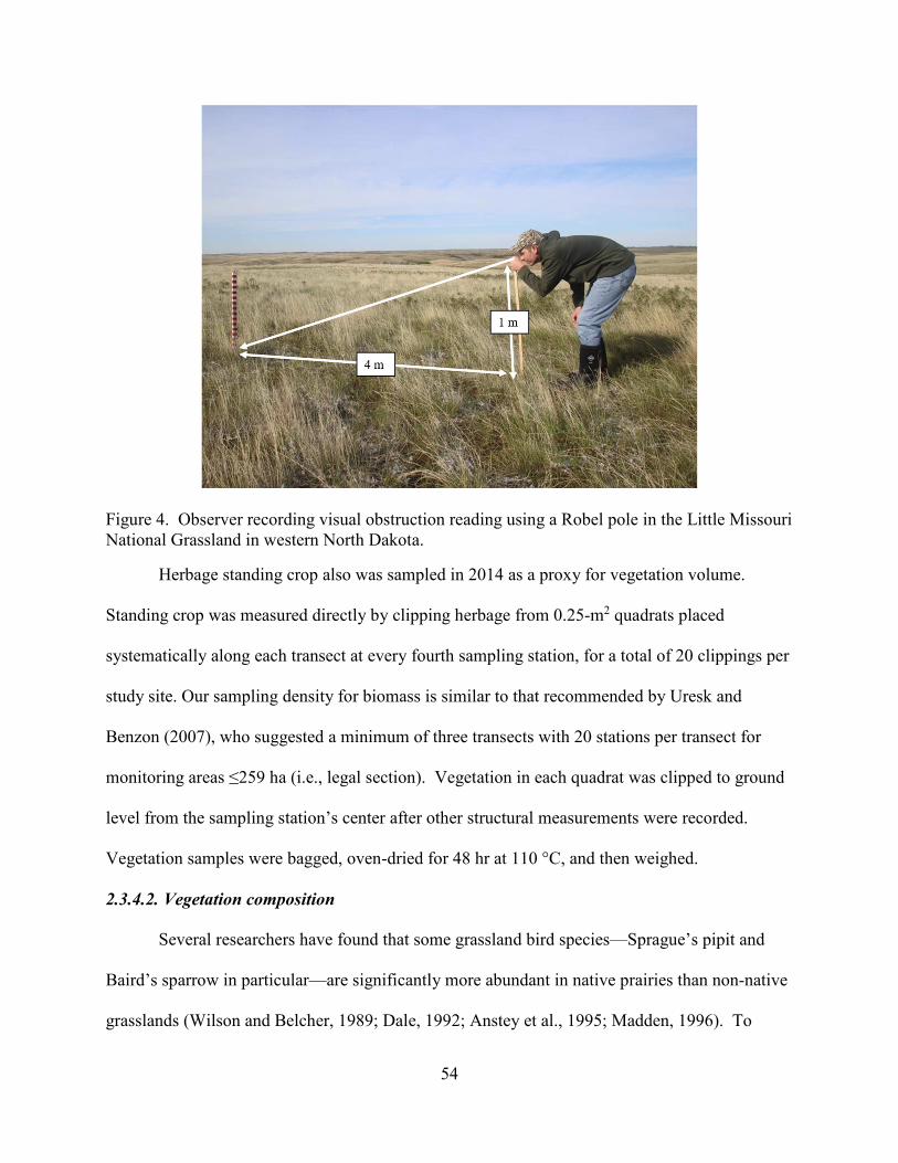
54
Figure 4. Observer recording visual obstruction reading using a Robel pole in the Little Missouri National Grassland in western North Dakota.
Herbage standing crop also was sampled in 2014 as a proxy for vegetation volume.
Standing crop was measured directly by clipping herbage from 0.25-m2 quadrats placed
systematically along each transect at every fourth sampling station, for a total of 20 clippings per
study site. Our sampling density for biomass is similar to that recommended by Uresk and
Benzon (2007), who suggested a minimum of three transects with 20 stations per transect for
monitoring areas ≤259 ha (i.e., legal section). Vegetation in each quadrat was clipped to ground
level from the sampling station’s center after other structural measurements were recorded.
Vegetation samples were bagged, oven-dried for 48 hr at 110 °C, and then weighed.
2.3.4.2. Vegetation composition
Several researchers have found that some grassland bird species—Sprague’s pipit and
Baird’s sparrow in particular—are significantly more abundant in native prairies than non-native
grasslands (Wilson and Belcher, 1989; Dale, 1992; Anstey et al., 1995; Madden, 1996). To

55
assess this assertion, we characterized the vegetation species composition of 57 study sites using
a modified Whittaker plot (Stohlgren et al., 1995; fig. 5). We did not survey three of our study
sites due to logistical constraints. Given that species composition does not vary appreciably
from one year to the next in grasslands (Gibson and Hulbert, 1987; Tilman and Downing, 1994;
DeKeyser et al., 2015), floristic composition was measured only once in the two field seasons,
one-half of the study sites in the first year and one-half during the second year. Three 1,000-m2
Whittaker plots were sampled in each quarter-section. Each Whittaker plot measures 20 × 50 m
(1,000 m2) and contained nested subplots of three different sizes. A 5 × 20-m (100-m2) subplot
was placed in the plot’s center, and two 2 × 5-m (10-m2) subplots were placed in opposite
corners of the plot. Presence/absence data were collected for the 10-m2, 100-m2, and 1,000-m2
subplots. There also was a total of ten 0.5-m × 2-m (1-m2) “microplots”. Six of the microplots
were arranged systematically inside and adjacent to the 1,000-m2 plot perimeter, and the other
four were arranged systematically outside and adjacent to the 100-m2 subplot perimeter. Percent
cover of all species and substrate variables (e.g., bare ground, litter) was visually estimated to the
nearest 1% within the microplots. Species that did not comprise 1% of the microplot were given
a value of 0.1%. Using ArcGIS (10.2.2 ESRI, Redlands, California), we placed ten randomized
points at each site to be used as the starting point for each plot. Using their best judgment,
observers would choose three points that were spatially widespread, did not fall within non-
grassland features (e.g., woody draws), and gave a good representation of the entire quarter-
section’s vegetation composition within grasslands. Once on the point, a random number
generator was used to obtain a directional bearing on which the plot would be oriented.

56
Figure 5. The layout of Modified-Whittaker plot used in this study to quantify plant species composition in the Little Missouri National Grassland, 2014 and 2015 (Stohlgren et al., 1995).
2.3.5. Statistical analyses
Breeding bird densities were calculated as the number of indicated breeding pairs
observed per 100 ha and were log-transformed (loge [bird density+1]) to normalize the data for
analyses. Bird data were averaged by year between the early and late-season total-area counts.
Due to time constraints, approximately one-half of the bird surveys occurred late into the
breeding season in 2014 (i.e., early August). These late-season surveys were dropped from
analyses because they occurred outside of the peak breeding season for birds in North Dakota
(Igl and Johnson, 1997). However, we retained the late observations of Sprague’s pipits because
they have two periods (bimodal) of breeding activity in North Dakota, the first from late April to
early June and the second from mid-July to early September (Stewart, 1975). Structural

57
vegetation variables (i.e., VOR, maximum height, litter depth, and biomass) were averaged for
each study site by year between the two survey periods. Density of oil wells, length of roads
(km), and percentage of grassland within a 1.6 km buffer of the quarter-section were used to
assess the level of disturbance in the surrounding landscape (i.e., landscape-level models). To
calculate oil-well densities, we only included the following well statuses as described by the
North Dakota Oil and Gas Commission (2016): active, drilling, inactive (≤ 12 months), not
completed, and temporarily abandoned. Percent coverages of bare ground, litter, Kentucky
bluegrass (Poa pratensis), and crested wheatgrass were calculated as an average of all cover
estimates from the Whittaker microplots. We included percent coverage of Kentucky bluegrass
and crested wheatgrass in our final analyses because literature suggested that these variables
influence sensitive grassland bird presence or abundance (Wilson and Belcher, 1989).
We also calculated a Floristic Quality Index (FQI) (NGPFQAP, 2001) for each site using
plant presence/absence data collected using the Whittaker subplots. Floristic quality assessments
assign a rating to each plant species that reflects the fundamental conservatism that the species
exhibits for natural habitats. We used a list of coefficients of conservatism (C values) developed
for the Dakotas by the Northern Great Plains Floristic Quality Assessment Panel (2001). C
values represent a plant species’ pattern of occurrence (i.e., common or rare) and if it is natural-
area dependent. C values range from 0-10. Ubiquitous species are given a low C value, and
species that exhibit specific adaptations are given a higher C value. The FQI is obtained by
multiplying mean C by the square root of the number of native species present. Thus, the FQI is
a weighted species-richness estimate that uses a square root transformation of the number of
native species present to limit the influence of area alone on species richness (Swink, 1974). We

58
calculated FQI using the Universal Floristic Quality Assessment Calculator (Freyman et al.,
2015).
Other researchers have detected a strong relationship between VOR and standing crop
(Robel et al., 1970; Vermeire and Gillen, 2001; Woehl, 2010). Based on the recommendation of
Vermeire and Gillen (2001), we ran a regression at the site level to explore the relationship
between standing crop and VOR. Regression models based on the site—rather than individual
observations—account for less variation because the true area measured by VOR is unknown, 3-
dimensional, and may vary among points; whereas quadrat size is 2-dimensional and consistent
among points. Models developed at the site level reduce this source of error by averaging both
VOR and standing crop over many individual points (Vermeire and Gillen, 2001). Mean
standing crop was calculated for the second year of the study by entering mean VOR’s into the
regression model. Definitions of all explanatory variables can be found in Table 1.
Table 1. Covariate abbreviations and corresponding descriptions for landscape and site-specific variables recorded at study sites in the Little Missouri National Grassland in western North Dakota, 2014 and 2015.
Variable type
Covariate abbreviation. Description
Landscape Percent.Grass Percentage grassland (e.g., range, hayland) within 1.6 km of site boundary.
Wells Well density (number of wells) within 1.6 km of site boundary. Roads Total road length (km) within 1.6 km of site boundary.
Site-specific Ltr.Depth Litter depth (cm).
Height Maximum vegetation height (cm) within 15 cm of Robel pole. AvVOR Average visual obstruction reading (cm). kgha Standing crop or biomass (kg per ha). Percent.AGCI Percentage cover of crested wheatgrass. Percent.POPR Percentage cover of Kentucky bluegrass. Percent.BG Percentage cover of bare ground. Percent.Litter Percentage cover of litter. FQI Floristic Quality Index. Slope Average percent slope of quarter-section.

59
We selected a suite of 12 grassland bird species to evaluate the effects of landscape and
site-specific variables on breeding bird densities: sharp-tailed grouse (Tympanuchus
phasianellus), upland sandpiper (Bartramia longicauda), horned lark (Eremophila alpestris),
Sprague’s pipit, clay-colored sparrow (Spizella pallida), field sparrow (Spizella pusilla), vesper
sparrow (Pooecetes gramineus), grasshopper sparrow (Ammodramus savannarum), Baird’s
sparrow, chestnut-collared longspur (Calcarius ornatus), bobolink, and western meadowlark
(Sturnella neglecta). We used an information-theoretic approach (Burnham and Anderson,
2002) to model individual bird species’ abundances against landscape factors (i.e., percent
grassland, length of roads, and oil well density, all within 1.6 km of the border of the quarter-
section) and site-specific factors (i.e., slope, VOR, maximum height, litter depth, and percentage
cover of bare ground, litter, Kentucky bluegrass, and crested wheatgrass). Models were
formulated as general linear models (GLMs) with an assumed Gaussian distribution based on an
ln(y + 1) transformation. We ranked models using Akaike’s Information Criteria (AIC)
corrected for small sample size (AICc) by computing the difference (Δi) between the model with
the smallest AICc and the model with the next smallest AICc (Burnham and Anderson, 2002). In
general, models with Δi ≤ 2 have substantial support, those with Δi of 4-7 have considerably less
support, and those with Δi >10 have essentially no support (Burnham and Anderson, 2002).
Because AICc is a relative measure, Burnham and Anderson (1998) recommended calculating the
AIC differences—or delta AIC (Δi = AICc, i - minAICc)—for each candidate model. The best
model has a Δi = 0. Akaike weights (ωi)—relative likelihood of a model—are also reported. The
relative importance of each model was assessed by computing Akaike’s model weights (ωi) and
60
we used root-mean-squared errors (RMSE) and adjusted R2 (Adj. R2) to assess the goodness-of-
fit of the final model(s).
Because we had limited information on which predictors might be useful a priori, we
took a two-step approach for deriving potential plausible models. Following habitat selection as
advocated by Johnson (1980), in the first stage, we looked at higher-level selection by examining
which of three landscape predictors might explain abundance of bird species using a suite of
eleven plausible models (Table 2). Year was included in all candidate models (except the null
model), regardless of its importance, because grassland bird populations in this region are known
to exhibit considerable annual variability in abundance from year-to-year on any particular site
(Igl and Johnson, 1997, 1999; Igl et al., 2008). In the second stage, uncorrelated site-specific
variables were then added to the best model from the landscape models to see if they improved
the model fit (Table 3). Overall, 25 site-specific plausible models were considered. Because
bird abundance and covariates, particularly site, can vary widely from year-to-year on each of the
sites, we assumed independence. To account for variation in the strength of relationships
between years, we included interaction terms between year and potential landscape and/or site-
specific variables. Bivariate plots by year were used as a descriptive method to better understand
the strength and direction of any relationships between bird abundance and covariates deemed
useful from the modeling effort. All statistical analyses were conducted in Program R (version
3.2.3; R Core Team 2015). The following R packages were used: “AICcmodavg” (Mazerolle,
2016), “MuMIn” (Barton, 2016), and “vegan” (Oksanen et al., 2016).
We also used the aforementioned GLM modeling selection to assess the effects of
explanatory variables on overall grassland bird diversity by calculating Shannon Diversity (H)
and using it as the dependent variable in the models. We restricted our analysis to the 12 most

61
common grassland birds detected on our sites. This approach allowed for simple interpretation
of the effects of the 13 explanatory variables on grassland bird diversity.
Table 2. Plausible models using landscape-level variables including well density (Wells), total length of roads (Roads), and percentage grass within 1.6 km of quarter-section edge (Percent.Grass). Refer to Table 1 for covariate descriptions.
Model No. Model description 1 Null 2 Year 3 Year + Wells 4 Year + Wells + Year×Wells 5 Year + Roads 6 Year + Roads + Year×Roads 7 Year + Percent.Grass 8 Year + Percent.Grass + Year×Percent.Grass 9 Year + Year×Percent.Grass + Year×Wells 10 Year + Year×Percent.Grass + Year×Roads 11 Year + Year×Roads + Year×Wells
Table 3. Plausible models using site-specific variables including average visual obstruction reading (AvVOR), percent slope (Slope), Native Floristic Quality Index (Native.FQI), and percentage cover of crested wheatgrass (Percent.AGCR), Kentucky bluegrass (Percent.POPR), bare ground (Percent.BG), and litter (Percent.Litter). Refer to Table 1 for covariate descriptions.
Model No. Model description 12 Best + AvVOR 13 Best + AvVOR + Year×AvVOR 14 Best + Slope 15 Best + Slope + Year×Slope 16 Best + FQI 17 Best + FQI + Year×FQI 18 Best + Percent.AGCR 19 Best + Percent.AGCR + Year×Percent.AGCR 20 Best + Percent.POPR 21 Best + Percent.POPR + Year×Percent.POPR 22 Best + Percent.BG 23 Best + Percent.BG + Year×Percent.BG 24 Best + Percent.Litter 25 Best + Percent.Litter + Year×Percent.Litter 26 Best + Ltr.Depth 27 Best + Ltr.Depth + Year×Ltr.Depth

62
2.4. Results
2.4.1. General
Average herbaceous standing crop among sites ranged from 846 to 2406 kg per ha. We
used the slope and intercept of the regression model to calculate standing crop estimates for 2015
(Fig. 6).
Figure 6. Linear regression plot between mean standing crop (biomass) and mean visual obstruction readings (VOR) with 95% confidence intervals for 60 quarter-section sites in the Little Missouri National Grassland, 2014 and 2015.
Patterns of correlation among the 13 explanatory variables were explored by calculating
Pearson’s correlation coefficients. The following explanatory variables were found to be
correlated (r ≥ 40%) (Table 4): VOR, maximum vegetation height, and biomass; FQI and percent

63
cover of crested wheatgrass; and percent bare ground and percent litter cover. Accordingly, we
did not include any of the correlated variables within the same plausible models. VOR was used
in place of vegetation height and biomass in the models because height and biomass were highly
correlated with VOR (r ≥ 70%). Summary statistics for the 13 explanatory variables can be
found in Table 4.
Figure 7. Correlation heatmap with Pearson correlation coefficients for landscape and site-specific covariates (n = 57). Positive correlations are displayed in orange and negative correlations are in brown. Color intensity is proportional to the correlation.
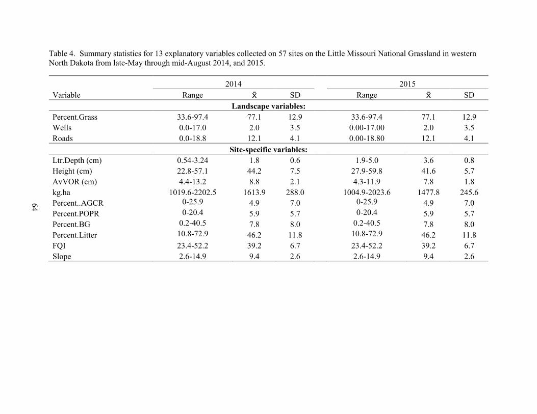
64
Table 4. Summary statistics for 13 explanatory variables collected on 57 sites on the Little Missouri National Grassland in western North Dakota from late-May through mid-August 2014, and 2015.
2014 2015 Variable Range SD Range SD
Landscape variables:
Percent.Grass 33.6-97.4 77.1 12.9 33.6-97.4 77.1 12.9 Wells 0.0-17.0 2.0 3.5 0.00-17.00 2.0 3.5 Roads 0.0-18.8 12.1 4.1 0.00-18.80 12.1 4.1
Site-specific variables:
Ltr.Depth (cm) 0.54-3.24 1.8 0.6 1.9-5.0 3.6 0.8 Height (cm) 22.8-57.1 44.2 7.5 27.9-59.8 41.6 5.7 AvVOR (cm) 4.4-13.2 8.8 2.1 4.3-11.9 7.8 1.8 kg.ha 1019.6-2202.5 1613.9 288.0 1004.9-2023.6 1477.8 245.6 Percent..AGCR 0-25.9 4.9 7.0 0-25.9 4.9 7.0 Percent.POPR 0-20.4 5.9 5.7 0-20.4 5.9 5.7 Percent.BG 0.2-40.5 7.8 8.0 0.2-40.5 7.8 8.0 Percent.Litter 10.8-72.9 46.2 11.8 10.8-72.9 46.2 11.8 FQI 23.4-52.2 39.2 6.7 23.4-52.2 39.2 6.7 Slope 2.6-14.9 9.4 2.6 2.6-14.9 9.4 2.6

65
During the breeding seasons of 2014 and 2015, we detected 69 and 76 bird species,
respectively. We observed 7,789 breeding pairs representing 82 bird species over the course of
the study (Table A2). The most frequently observed species were the grasshopper sparrow and
western meadowlark, which were detected on 100% of the study sites, vesper sparrow (97%),
and mourning dove (Zenaida macroura [88%]). The 20 most frequently observed species are
summarized in Table 5. The suite of 12 grassland birds selected for further analyses all occurred
on >20% of the study sites. Sensitive species detected in USFS Region 1 over the duration of
this monitoring program include: burrowing owl (Athene cunicularia), loggerhead shrike (Lanius
ludovicianus), Sprague’s pipit and Baird’s sparrow. Other birds we observed that are considered
sensitive by the USFS were burrowing owl (Athene cunicularia) and loggerhead shrike (Lanius
ludovicianus). We also observed two breeding pairs of long-billed curlew (Numenius
americanus) near one of our study sites during both years of the study; however, they were never
observed using any of the study sites during our breeding bird surveys.
We recorded 195 plant species in 171 modified Whittaker plots on 57 study sites in 2014
and 2015 (Table A3). Native species accounted for 86.7% (169 species) of the total plant
community, whereas non-native species accounted for 13.3% (26 species) of the total plant
community. The average Native Mean C value for the study area is 5.1 and the average FQI is
39.2. Forbs comprised 65.6% of the plant community; grasses and sedges combined for 20.5%
of the plant community; shrubs and trees accounted for 11.8% of the plant community; and ferns,
bryophytes, and vines, combined for 2% of the plant community. FQI for individual sites ranged
from 23.4 to 52.2 (Table A4). The five vegetation composition variables with the highest
percent cover (averaged across all sites) were: litter (46.4%), bare ground (7.8%), western
wheatgrass (5.9%), Kentucky bluegrass (5.9%), and crested wheatgrass (4.7%)

66
Table 5. Summary statistics for the 20 most frequently observed breeding bird species during surveys conducted on the Little Missouri National Grassland in western North Dakota between 23 May to 25 July 2014 and 19 May to 17 July 2015. The species are ordered by frequency of occurrence.
Species Sites observed1
Frequency occurrence
Average densities (no. pairs per 100 ha)
Density SD
Density range
Grasshopper sparrow 119 1.00 30.92 12.8 3.9-65.0 Western meadowlark 119 1.00 22.53 8.1 0.8-38.0 Vesper sparrow 116 0.97 6.80 4.4 0.0-22.8 Mourning Dove 108 0.88 2.28 1.8 0.0-7.9 Eastern kingbird 100 0.82 2.18 1.8 0.0-7.7 Bobolink 95 0.77 4.22 4.2 0.0-17.0 Brown-headed cowbird 92 0.75 1.83 1.9 0.0-9.3 Clay-colored sparrow 91 0.74 3.32 5.0 0.0-28.3 Sharp-tailed grouse 89 0.72 1.70 2.0 0.0-11.6 Yellow warbler 88 0.71 2.54 2.6 0.0-14.0 Spotted towhee 81 0.66 2.34 2.9 0.0-14.8 Field sparrow 79 0.64 2.27 2.7 0.0-14.8 Upland sandpiper 75 0.61 1.23 1.3 0.0-4.7 Brown thrasher 65 0.52 0.79 1.0 0.0-3.8 Horned lark 58 0.46 1.85 3.5 0.0-18.9 House wren 52 0.41 0.98 1.6 0.0-7.0 Red-winged blackbird 47 0.37 0.94 2.2 0.0-14.3 Sprague's pipit 44 0.34 1.61 3.1 0.0-13.2 Baird's sparrow 40 0.31 1.31 2.8 0.0-13.9 Chestnut-collared longspur 32 0.24 1.66 4.9 0.0-33.2 1 n = 60 site-by-year combination.

67
2.4.2. Modeling results
2.4.2.1. Grassland bird community
The best supported and most parsimonious landscape model for grassland bird diversity
had weak evidence (ωi = 0.38, R2 = 0.06) that diversity is associated with Percent.Grass (Table
6). One site-specific variable (VOR) improved the best-supported landscape model (ωi = 0.51),
and explained 12% of the variation in grassland bird diversity. The best-supported site-specific
model did not include any Year interactions, therefore the relationship between grassland bird
diversity and the explanatory variables did not vary from year-to-year. Grassland bird diversity
showed a slight decline with increasing percentage cover of grassland within 1.6 km of the site
edge and average VOR (Fig. 8).
2.4.2.2. Sharp-tailed grouse
The best supported and most parsimonious landscape model for the sharp-tailed grouse
included Year and Wells (Table 7). However, the evidence that sharp-tailed grouse abundance is
a function of Year and Wells is weak (ωi = 0.23, R2 = 0.03). One site-specific variable
(Ltr.Depth) improved the best-supported landscape model relative to other models (ωi = 0.39),
but only explained 7% of the variation in sharp-tailed grouse abundance. The best site-specific
model did not include any Year interactions, thus the relationship between sharp-tailed grouse
abundance and Ltr.Depth did not vary substantially from year-to-year. Although many sites had
zero sharp-tailed grouse across the range of Wells and Ltr.Depth, sharp-tailed grouse abundance
declined with increasing well density (Fig. 9). Sharp-tailed grouse abundance slightly increased
with increasing litter depth in 2014 and 2015.

68
Table 6. Model-selection results for models relating grassland bird diversity (Shannon [H]) to landscape and site-specific habitat variables in the Little Missouri National Grassland in western North Dakota, 2014 and 2015 (n=114; sorted by Δi). Models were ranked according to Akaike’s information criterion adjusted for small sample size (AICc). Variable definitions are given in Table 1.
Model K1 AICC Δi
2 ωi3 RMSE4 Adj. R2
Landscape models:
mod7 Year + Percent.Grass 4 -307.2 0.0 0.38344 0.06062 0.06 mod8 Year + Percent.Grass + Year * Percent.Grass 5 -305.3 2.0 0.14438 0.06056 0.05 mod10 Year + Year * Percent.Grass + Year * Roads 7 -305.1 2.2 0.12933 0.05943 0.07 mod5 Year + Roads 4 -304 3.3 0.07446 0.06150 0.03 mod9 Year + Year * Percent.Grass + Year * Wells 7 -303.8 3.4 0.06966 0.05975 0.06 mod2 Year 3 -303.3 4.0 0.05233 0.06227 0.02 mod4 Year + Wells + Year * Wells 5 -302.8 4.4 0.04169 0.06122 0.03 mod1 Null 2 -302.3 5.0 0.03195 0.06312 0.0 mod3 Year + Wells 4 -301.9 5.3 0.02646 0.06206 0.02 mod6 Year + Roads + Year * Roads 5 -301.8 5.5 0.02493 0.06150 0.02 mod11 Year + Year * Roads + Year * Wells 7 -301.5 5.8 0.02138 0.06037 0.04
Best landscape model plus site-specific models:
mod12 Year + Percent.Grass + AvVOR 5 -313.2 0.0 0.50792 0.05850 0.12 mod13 Year + Percent.Grass + AvVOR + Year * AvVOR 6 -311 2.2 0.17025 0.05849 0.11 mod24 Year + Percent.Grass + Percent.Litter 5 -309.1 4.1 0.06557 0.05956 0.09 mod17 Year + Percent.Grass + Native.FQI + Year * Native.FQI 6 -308.9 4.3 0.05973 0.05903 0.09 mod16 Year + Percent.Grass + Native.FQI 5 -308.2 4.9 0.04305 0.05978 0.08 mod26 Year + Percent.Grass + Ltr.Depth 5 -307.8 5.4 0.03479 0.05989 0.08 mod7 Year + Percent.Grass 4 -307.2 5.9 0.02636 0.06062 0.06 mod25 Year + Percent.Grass + Percent.Litter + Year * Percent.Litter 6 -307.1 6.1 0.02435 0.05950 0.08 mod27 Year + Percent.Grass + Ltr.Depth + Year * Ltr.Depth 6 -305.6 7.5 0.01177 0.05988 0.07 mod18 Year + Percent.Grass + Percent.AGCR 5 -305.5 7.6 0.01123 0.06049 0.06 mod22 Year + Percent.Grass + Percent.BG 5 -305.3 7.8 0.01008 0.06055 0.05 mod14 Year + Percent.Grass + Slope 5 -305.3 7.9 0.00983 0.06056 0.05 mod20 Year + Percent.Grass + Percent.POPR 5 -305.1 8.1 0.00900 0.06061 0.05 mod23 Year + Percent.Grass + Percent.BG + Year * Percent.BG 6 -303.9 9.3 0.00487 0.06034 0.05 mod19 Year + Percent.Grass + Percent.AGCR + Year * Percent.AGCR 6 -303.8 9.4 0.00464 0.06037 0.05 mod15 Year + Percent.Grass + Slope + Year * Slope 6 -303.3 9.9 0.00359 0.06050 0.05 mod21 Year + Percent.Grass + Percent.POPR + Year * Percent.POPR 6 -302.9 10.3 0.00296 0.06061 0.04 1 Number of parameters. 2 Delta AIC (measure of each model relative to the best model). 3 Akaike weights (measure of the strength of evidence for each model). 4 Root mean square error.

69
Figure 8. Model results showing relationship (black line with red-dashed 95% confidence intervals) between grassland bird diversity (Shannon [H]) and percentage grassland and visual obstruction reading (cm).

70
Table 7. Model-selection results for models relating sharp-tailed grouse abundance to landscape and site-specific habitat variables in the Little Missouri National Grassland in western North Dakota, 2014 and 2015 (n=114; sorted by Δi). Models were ranked according to Akaike’s information criterion adjusted for small sample size (AICc). Variable definitions are given in Table 1.
Model K1 AICC Δi
2 ωi3 RMSE4 Adj. R2
Landscape models:
mod3 Year + Wells 4 223.6 0.0 0.23247 0.62191 0.03 mod7 Year + Percent.Grass 4 224.2 0.6 0.17222 0.62355 0.02 mod2 Year 3 224.3 0.7 0.16065 0.62983 0.01 mod1 Null 2 224.6 1.0 0.14256 0.63636 0.00 mod4 Year + Wells + Year * Wells 5 225.6 2.0 0.08497 0.62143 0.02 mod8 Year + Percent.Grass + Year * Percent.Grass 5 225.6 2.0 0.08485 0.62144 0.02 mod5 Year + Roads 4 226.4 2.8 0.05639 0.62968 0.00 mod9 Year + Year * Percent.Grass + Year * Wells 7 227.8 4.3 0.02768 0.61530 0.02 mod6 Year + Roads + Year * Roads 5 228.6 5.0 0.01889 0.62968 -0.01 mod10 Year + Year * Percent.Grass + Year * Roads 7 229.9 6.3 0.00983 0.62092 0.00 mod11 Year + Year * Roads + Year * Wells 7 230.0 6.4 0.00948 0.62111 0.00
Best landscape model plus site-specific models:
mod26 Year + Wells + Ltr.Depth 5 219.6 0.0 0.38544 0.60523 0.07 mod27 Year + Wells + Ltr.Depth + Year * Ltr.Depth 6 221.5 1.9 0.15038 0.60431 0.07 mod16 Year + Wells + FQI 5 222.4 2.8 0.09576 0.61267 0.05 mod3 Year + Wells 4 223.6 4.0 0.05192 0.62191 0.03 mod21 Year + Wells + Percent.POPR + Year * Percent.POPR 6 223.7 4.1 0.04967 0.61021 0.05 mod12 Year + Wells + AvVOR 5 223.7 4.2 0.04814 0.61637 0.04 mod24 Year + Wells + Percent.Litter 5 223.9 4.3 0.04422 0.61683 0.03 mod17 Year + Wells + FQI + Year * FQI 6 224.3 4.7 0.03614 0.61191 0.04 mod20 Year + Wells + Percent.POPR 5 225.4 5.8 0.02108 0.62085 0.02 mod14 Year + Wells + Slope 5 225.5 5.9 0.01988 0.62117 0.02 mod18 Year + Wells + Percent.AGCR 5 225.7 6.2 0.01778 0.62178 0.02 mod22 Year + Wells + Percent.BG 5 225.8 6.2 0.01738 0.62191 0.02 mod19 Year + Wells + Percent.AGCR + Year * Percent.AGCR 6 225.9 6.3 0.01640 0.61617 0.03 mod13 Year + Wells + AvVOR + Year * AvVOR 6 225.9 6.3 0.01619 0.61624 0.03 mod25 Year + Wells + Percent.Litter + Year * Percent.Litter 6 226.1 6.5 0.01476 0.61674 0.03 mod23 Year + Wells + Percent.BG + Year * Percent.BG 6 227.3 7.7 0.00833 0.61984 0.02 mod15 Year + Wells + Slope + Year * Slope 6 227.7 8.2 0.00653 0.62117 0.01 1 Number of parameters. 2 Delta AIC (measure of each model relative to the best model). 3 Akaike weights (measure of the strength of evidence for each model). 4 Root mean square error.

71
Figure 9. Model results showing relationship (black line with red-dashed 95% confidence intervals) between sharp-tailed grouse abundance and well density and litter depth (cm). Only strongly supported relationships are shown.

72
2.4.2.3. Upland sandpiper
The landscape model for upland sandpiper indicated that sandpiper densities were a
function of Year and Percent.Grass (ωi = 0.54, Adj. R2 = 0.10). The association, albeit weak,
with Year and Percent.Grass indicates that Percent.Grass affects upland sandpiper abundance
consistently between the two years (Table 8). One site-specific variable (Percent.BG) improved
the best-supported landscape model (ωi = 0.47), which explained 16% of the variation in upland
sandpiper abundance. The best site-specific model did not include an interaction between
Percent.Grass or Percent.BG and Year, indicating that upland sandpiper densities were
associated with Percent.Grass and Percent.BG but the direction and strength of the relationship
did not vary with year. There is some evidence of an interaction between Year and Percent.BG
(ωi = 0.35, Adj. R2 = 0.17), but the site-specific model with the most weight and lowest Δi
included only Year, Percent.Grass, and Percent.BG. Although many sites had zero abundance
across the range of Percent.Grass and Percent.BG, upland sandpiper abundance tended to
increase consistently with increasing grassland cover in the surrounding landscape (i.e., within
1.6 km of the study site) and increased with increasing bare ground cover in both years (Fig. 10).
2.4.2.4. Horned lark
Only Year was associated with horned lark densities at the landscape level (Table 9).
There is good evidence suggesting that horned lark densities are associated with Year and
Ltr.Depth (ωi = 0.70, Adj. R2 = 0.30) at the site-specific level. Although horned larks were
absent from many sites across the range of Ltr.Depth, horned lark abundance tended to decrease
with increasing litter depth with this relationship being fairly consistent between the two years
(Fig. 11).

73
Table 8. Model-selection results for models relating upland sandpiper abundance to landscape and site-specific habitat variables in the Little Missouri National Grassland in western North Dakota, 2014 and 2015 (n=114; sorted by Δi). Models were ranked according to Akaike’s information criterion adjusted for small sample size (AICc). Variable definitions are given in Table 1.
Model K1 AICC Δi
2 ωi3 RMSE4 Adj. R2
Landscape models:
mod7 Year + Percent.Grass 4 214.4 0.0 0.54234 0.59730 0.10 mod10 Year + Year * Percent.Grass + Year * Roads 7 216.1 1.7 0.22655 0.58448 0.11 mod8 Year + Percent.Grass + Year * Percent.Grass 5 216.5 2.1 0.18558 0.59718 0.09 mod9 Year + Year * Percent.Grass + Year * Wells 7 220.5 6.2 0.02500 0.59589 0.08 mod5 Year + Roads 4 223.9 9.6 0.00456 0.62287 0.02 mod2 Year 3 224.1 9.7 0.00420 0.62922 0.01 mod1 Null 2 224.2 9.9 0.00393 0.63544 0.00 mod3 Year + Wells 4 224.4 10.0 0.00362 0.62413 0.02 mod6 Year + Roads + Year * Roads 5 225.6 11.2 0.00200 0.62141 0.02 mod4 Year + Wells + Year * Wells 5 226.2 11.8 0.00145 0.62315 0.01 mod11 Year + Year * Roads + Year * Wells 7 227.5 13.1 0.00077 0.61440 0.02
Best landscape model plus site-specific models:
mod22 Year + Percent.Grass + Percent.BG 5 207.1 0.0 0.47086 0.57302 0.16 mod23 Year + Percent.Grass + Percent.BG + Year * Percent.BG 6 207.7 0.6 0.35714 0.56882 0.17 mod18 Year + Percent.Grass + Percent.AGCR 5 210.8 3.7 0.07531 0.58230 0.14 mod19 Year + Percent.Grass + Percent.AGCR + Year * Percent.AGCR 6 212.7 5.6 0.02936 0.58142 0.13 mod24 Year + Percent.Grass + Percent.Litter 5 213.8 6.7 0.01662 0.59007 0.11 mod7 Year + Percent.Grass 4 214.4 7.3 0.01240 0.59730 0.10 mod25 Year + Percent.Grass + Percent.Litter + Year * Percent.Litter 6 215.8 8.6 0.00626 0.58935 0.11 mod14 Year + Percent.Grass + Slope 5 216.2 9.1 0.00504 0.59628 0.10 mod26 Year + Percent.Grass + Ltr.Depth 5 216.3 9.1 0.00486 0.59647 0.09 mod12 Year + Percent.Grass + AvVOR 5 216.3 9.2 0.00467 0.59668 0.09 mod20 Year + Percent.Grass + Percent.POPR 5 216.5 9.4 0.00421 0.59722 0.09 mod16 Year + Percent.Grass + FQI 5 216.6 9.5 0.00416 0.59729 0.09 mod15 Year + Percent.Grass + Slope + Year * Slope 6 217.8 10.6 0.00230 0.59457 0.09 mod17 Year + Percent.Grass + FQI + Year * FQI 6 218.1 11.0 0.00191 0.59553 0.09 mod13 Year + Percent.Grass + AvVOR + Year * AvVOR 6 218.3 11.2 0.00174 0.59603 0.09 mod27 Year + Percent.Grass + Ltr.Depth + Year * Ltr.Depth 6 218.5 11.4 0.00160 0.59644 0.09 mod21 Year + Percent.Grass + Percent.POPR + Year * Percent.POPR 6 218.5 11.4 0.00157 0.59654 0.09 1 Number of parameters. 2 Delta AIC (measure of each model relative to the best model). 3 Akaike weights (measure of the strength of evidence for each model). 4 Root mean square error.

74
Figure 10. Model results showing relationship (black line with red-dashed 95% confidence intervals) between upland sandpiper abundance and percentage grassland and bare ground.

75
Table 9. Model-selection results for models relating horned lark abundance to landscape and site-specific habitat variables in the Little Missouri National Grassland in western North Dakota, 2014 and 2015 (n=114; sorted by Δi). Models were ranked according to Akaike’s information criterion adjusted for small sample size (AICc). Variable definitions are given in Table 1.
Model K1 AICC Δi
2 ωi3 RMSE4 Adj. R2
Landscape models:
mod2 Year 3 285.5 0.0 0.22260 0.82353 0.01 mod1 Null 2 285.5 0.1 0.21655 0.83138 0.00 mod5 Year + Roads 4 286.5 1.0 0.13608 0.81933 0.01 mod3 Year + Wells 4 286.5 1.0 0.13538 0.81937 0.01 mod7 Year + Percent.Grass 4 287.4 1.9 0.08525 0.82270 0.00 mod6 Year + Roads + Year * Roads 5 287.5 2.1 0.07873 0.81541 0.01 mod4 Year + Wells + Year * Wells 5 288.5 3.1 0.04830 0.81891 0.00 mod8 Year + Percent.Grass + Year * Percent.Grass 5 288.9 3.5 0.03952 0.82035 0.00 mod11 Year + Year * Roads + Year * Wells 7 290.6 5.2 0.01681 0.81037 0.01 mod10 Year + Year * Percent.Grass + Year * Roads 7 291.4 6.0 0.01121 0.81326 0.00 mod9 Year + Year * Percent.Grass + Year * Wells 7 291.8 6.3 0.00957 0.81439 0.00
Best landscape model plus site-specific models:
mod26 Year + Ltr.Depth 4 246.7 0.0 0.69716 0.68821 0.30 mod27 Year + Ltr.Depth + Year * Ltr.Depth 5 248.6 1.9 0.26844 0.68736 0.30 mod13 Year + AvVOR + Year * AvVOR 5 253.8 7.1 0.02010 0.70317 0.27 mod12 Year + AvVOR 4 254.5 7.8 0.01430 0.71207 0.25 mod24 Year + Percent.Litter 4 278.8 32.1 0.00000 0.79222 0.08 mod25 Year + Percent.Litter + Year * Percent.Litter 5 280.7 34.0 0.00000 0.79132 0.07 mod14 Year + Slope 4 281.9 35.3 0.00000 0.80329 0.05 mod15 Year + Slope + Year * Slope 5 283.0 36.3 0.00000 0.79936 0.05 mod2 Year 3 285.5 38.8 0.00000 0.82353 0.01 mod22 Year + Percent.BG 4 285.6 38.9 0.00000 0.81628 0.02 mod18 Year + Percent.AGCR 4 285.6 38.9 0.00000 0.81636 0.02 mod20 Year + Percent.POPR 4 286.5 39.8 0.00000 0.81953 0.01 mod23 Year + Percent.BG + Year * Percent.BG 5 287.2 40.5 0.00000 0.81402 0.02 mod16 Year + FQI 4 287.5 40.8 0.00000 0.82307 0.00 mod19 Year + Percent.AGCR + Year * Percent.AGCR 5 287.7 41.0 0.00000 0.81578 0.01 mod21 Year + Percent.POPR + Year * Percent.POPR 5 288.5 41.8 0.00000 0.81889 0.00 mod17 Year + FQI + Year * FQI 5 288.9 42.2 0.00000 0.82013 0.00 1 Number of parameters. 2 Delta AIC (measure of each model relative to the best model). 3 Akaike weights (measure of the strength of evidence for each model). 4 Root mean square error.

76
Figure 11. Model results showing relationship (black line with red-dashed 95% confidence intervals) between horned lark abundance and litter depth.

77
2.4.2.5. Sprague’s pipit
For the Sprague’s pipit, the best supported and most parsimonious landscape model,
based on Δi and ωi, included Year and Roads (R2 = 0.13), indicating that Sprague’s pipit
abundance is weakly associated with roads and that this association is consistent between the two
years (Table 10). There is some evidence (ωi = 0.22, Adj. R2 = 0.12) that Sprague’s pipit
densities are associated with the interaction between Year and Roads, but the landscape model
with the most weight included only Year and Roads. One site-specific variable (AvVOR)
improved the landscape model (ωi = 0.60, R2 = 0.23). Within the range of roads and VOR
sampled, Sprague’s pipit abundance declines with increasing road densities and VOR. These
declines were fairly consistent from year-to-year (Fig. 12).
2.4.2.6. Clay-colored sparrow
For the clay-colored sparrow, the best supported and most parsimonious landscape model
included Year, the interaction between Year and Percent.Grass, and the interaction between Year
and Wells. This indicated that clay-colored sparrow abundance is associated with the percentage
of grassland and density of wells within 1.6 km of the study site and that this association varied
between the two years (Table 11). One site-specific variable (FQI) improved the best-supported
landscape model (ωi = 0.38, R2 = 0.31). The best site-specific model included all of the
interactions from the best landscape model but did not include interactions between the site-
specific variable (FQI) and Year, indicating that clay-colored sparrow densities were associated
with FQI and the strength of the relationship did not vary with year. Across the range of
grassland cover sampled, Clay-colored sparrow abundance decreased with increasing grassland
cover, especially in 2014 (Fig. 13). Abundance also tended to increase with increasing well
density and increasing FQI.

78
Table 10. Model-selection results for models relating Sprague’s pipit abundance to landscape and site-specific habitat variables in the Little Missouri National Grassland in western North Dakota, 2014 and 2015 (n=114; sorted by Δi). Models were ranked according to Akaike’s information criterion adjusted for small sample size (AICc). Variable definitions are given in Table 1.
Model K1 AICC Δi
2 ωi3 RMSE4 Adj. R2
Landscape models:
mod5 Year + Roads 4 274.1 0.0 0.67242 0.77618 0.13 mod6 Year + Roads + Year * Roads 5 276.3 2.2 0.22625 0.77614 0.12 mod10 Year + Year * Percent.Grass + Year * Roads 7 278.6 4.5 0.07252 0.76860 0.12 mod11 Year + Year * Roads + Year * Wells 7 280.6 6.4 0.02678 0.77535 0.11 mod1 Null 2 287.6 13.5 0.00078 0.83909 0.00 mod7 Year + Percent.Grass 4 288.3 14.2 0.00056 0.82593 0.01 mod2 Year 3 289.5 15.4 0.00030 0.83828 -0.01 mod8 Year + Percent.Grass + Year * Percent.Grass 5 290.4 16.3 0.00020 0.82565 0.01 mod3 Year + Wells 4 291.6 17.4 0.00011 0.83789 -0.02 mod4 Year + Wells + Year * Wells 5 293.6 19.4 0.00004 0.83717 -0.02 mod9 Year + Year * Percent.Grass + Year * Wells 7 294.5 20.4 0.00002 0.82433 -0.01
Best landscape model plus site-specific models:
mod12 Year + Roads + AvVOR 5 261.5 0.0 0.59542 0.72728 0.23 mod13 Year + Roads + AvVOR + Year * AvVOR 6 262.9 1.4 0.28838 0.72480 0.23 mod26 Year + Roads + Ltr.Depth 5 266.8 5.3 0.04182 0.74443 0.19 mod24 Year + Roads + Percent.Litter 5 267.2 5.8 0.03349 0.74588 0.19 mod27 Year + Roads + Ltr.Depth + Year * Ltr.Depth 6 268.9 7.5 0.01418 0.74421 0.18 mod25 Year + Roads + Percent.Litter + Year * Percent.Litter 6 269.2 7.8 0.01217 0.74521 0.18 mod14 Year + Roads + Slope 5 271.3 9.8 0.00437 0.75931 0.16 mod16 Year + Roads + FQI 5 271.6 10.1 0.00383 0.76020 0.16 mod17 Year + Roads + FQI + Year * FQI 6 272.7 11.3 0.00213 0.75668 0.16 mod15 Year + Roads + Slope + Year * Slope 6 273.5 12.1 0.00144 0.75931 0.15 mod5 Year + Roads 4 274.1 12.6 0.00107 0.77618 0.13 mod18 Year + Roads + Percent.AGCR 5 275.7 14.2 0.00049 0.77406 0.13 mod22 Year + Roads + Percent.BG 5 276.1 14.7 0.00039 0.77561 0.12 mod20 Year + Roads + Percent.POPR 5 276.2 14.7 0.00038 0.77579 0.12 mod19 Year + Roads + Percent.AGCR + Year * Percent.AGCR 6 277.9 16.4 0.00017 0.77385 0.12 mod21 Year + Roads + Percent.POPR + Year * Percent.POPR 6 278.1 16.7 0.00014 0.77485 0.12 mod23 Year + Roads + Percent.BG + Year * Percent.BG 6 278.3 16.8 0.00013 0.77543 0.11 1 Number of parameters. 2 Delta AIC (measure of each model relative to the best model). 3 Akaike weights (measure of the strength of evidence for each model). 4 Root mean square error.

79
Figure 12. Model results showing relationship (black line with red-dashed 95% confidence intervals) between Sprague’s pipit abundance and road length and visual obstruction reading.

80
Table 11. Model-selection results for models relating clay-colored sparrow abundance to landscape and site-specific habitat variables in the Little Missouri National Grassland in western North Dakota, 2014 and 2015 (n=114; sorted by Δi). Models were ranked according to Akaike’s information criterion adjusted for small sample size (AICc). Variable definitions are given in Table 1.
Model K1 AICC Δi
2 ωi3 RMSE4 Adj. R2
Landscape models:
mod9 Year + Year * Percent.Grass + Year * Wells 7 272.8 0.0 0.94035 0.74942 0.25 mod7 Year + Percent.Grass 4 279.4 6.6 0.03522 0.79429 0.18 mod8 Year + Percent.Grass + Year * Percent.Grass 5 281.5 8.7 0.01201 0.79416 0.17 mod3 Year + Wells 4 282.4 9.6 0.00790 0.79334 0.16 mod4 Year + Wells + Year * Wells 5 284.5 11.7 0.00269 0.80477 0.16 mod10 Year + Year * Percent.Grass + Year * Roads 7 285.8 13.0 0.00142 0.80465 0.15 mod11 Year + Year * Roads + Year * Wells 7 288.4 15.5 0.00040 0.80230 0.14 mod1 Null 2 299.7 26.9 0.00000 0.88465 0.00 mod2 Year 3 301.8 29.0 0.00000 0.88465 -0.01 mod5 Year + Roads 4 303.0 30.1 0.00000 0.88083 -0.01 mod6 Year + Roads + Year * Roads 5 305.1 32.3 0.00000 0.88080 -0.02
Best landscape model plus site-specific models:
mod16 Year + Year * Percent.Grass + Year * Wells + FQI 8 264.3 0.0 0.38695 0.71460 0.31 mod26 Year + Year * Percent.Grass + Year * Wells + Ltr.Depth 8 265.8 1.5 0.18401 0.71928 0.30 mod17 Year + Year * Percent.Grass + Year * Wells + FQI + Year * FQI 9 266.6 2.3 0.12021 0.71454 0.30 mod27 Year + Year * Percent.Grass + Year * Wells + Ltr.Depth + Year * Ltr.Depth 9 266.6 2.4 0.11883 0.71461 0.30 mod12 Year + Year * Percent.Grass + Year * Wells + AvVOR 8 267.2 2.9 0.09125 0.72372 0.29 mod18 Year + Year * Percent.Grass + Year * Wells + Percent.AGCR 8 269.0 4.8 0.03563 0.72971 0.28 mod13 Year + Year * Percent.Grass + Year * Wells + AvVOR + Year * AvVOR 9 269.3 5.1 0.03092 0.72310 0.29 mod19 Year + Year * Percent.Grass + Year * Wells + Percent.AGCR + Year * Percent.AGCR 9 271.0 6.8 0.01322 0.72851 0.28 mod9 Year + Year * Percent.Grass + Year * Wells 7 272.8 8.5 0.00544 0.74942 0.25 mod20 Year + Year * Percent.Grass + Year * Wells + Percent.POPR 8 273.4 9.1 0.00409 0.74371 0.25 mod22 Year + Year * Percent.Grass + Year * Wells + Percent.BG 8 274.7 10.4 0.00212 0.74800 0.24 mod14 Year + Year * Percent.Grass + Year * Wells + Slope 8 274.9 10.7 0.00186 0.74884 0.24 mod24 Year + Year * Percent.Grass + Year * Wells + Percent.Litter 8 275.0 10.8 0.00178 0.74916 0.24 mod21 Year + Year * Percent.Grass + Year * Wells + Percent.POPR + Year * Percent.POPR 9 275.6 11.4 0.00133 0.74335 0.25 mod25 Year + Year * Percent.Grass + Year * Wells + Percent.Litter + Year * Percent.Litter 9 276.5 12.2 0.00088 0.74606 0.24 mod15 Year + Year * Percent.Grass + Year * Wells + Slope + Year * Slope 9 276.7 12.4 0.00079 0.74677 0.24 mod23 Year + Year * Percent.Grass + Year * Wells + Percent.BG + Year * Percent.BG 9 276.9 12.6 0.00072 0.74737 0.24 1 Number of parameters. 2 Delta AIC (measure of each model relative to the best model). 3 Akaike weights (measure of the strength of evidence for each model). 4 Root mean square error.

81
Figure 13. Model results showing relationship (black line with red-dashed 95% confidence intervals) between clay-colored sparrow abundance and percentage grassland, well density, and FQI.

82
2.4.2.7. Field sparrow
The best supported and most parsimonious landscape model, albeit weak (ωi = 0.63, R2 =
0.07), for field sparrow abundance included Year and Percent.Grass (Table 12). One site-
specific variable (Percent.AGCR) improved the best-supported landscape model (ωi = 0.66).
However, the final model only explained 16% of variation in field sparrow abundance. The best
site-specific model did not include any interactions with year, and thus the relationship between
field sparrow abundance and the explanatory variables did not vary with year. Although many
sites had zero abundance across the range of Percent.Grass and Percent.AGCR, field sparrow
abundance tended to decline with increasing percentage of grassland in the surrounding
landscape and the percentage of crested wheatgrass at the site level (Fig. 14).
2.4.2.8. Vesper sparrow
The best supported and most parsimonious landscape model for the vesper sparrow based
on Δi and ωi, included Year and Wells (R2 = 0.07), indicating that vesper sparrow abundance is
weakly associated with the density of wells within 1.6 km of the study site and that this
association is fairly consistent between the two years (Table 13). One site-specific variable
(FQI) improved the best-supported landscape model (ωi = 0.24, R2 = 0.17). There also is
evidence that the association between vesper sparrow abundance and FQI varies from year-to-
year (ωi = 0.22, Adj. R2 = 0.18); however, the best model based on Δi does not include this
interaction. Although many sites had zero abundance across the range of Wells and FQI, vesper
sparrow abundance tended to decrease with increasing oil well density in the surrounding
landscape and FQI at the site level, with some tendency for the relationship to be stronger in
2015 (Fig. 15).

83
Table 12. Model-selection results for models relating field sparrow abundance to landscape and site-specific habitat variables in the Little Missouri National Grassland in western North Dakota, 2014 and 2015 (n=114; sorted by Δi). Models were ranked according to Akaike’s information criterion adjusted for small sample size (AICc). Variable definitions are given in Table 1.
Model K1 AICC Δi
2 ωi3 RMSE4 Adj. R2
Landscape models:
mod7 Year + Percent.Grass 4 284.0 0.0 0.63184 0.81044 0.07 mod8 Year + Percent.Grass + Year * Percent.Grass 5 285.9 1.9 0.23980 0.80955 0.06 mod10 Year + Year * Percent.Grass + Year * Roads 7 289.7 5.7 0.03566 0.80710 0.05 mod9 Year + Year * Percent.Grass + Year * Wells 7 289.9 5.9 0.03266 0.80773 0.05 mod1 Null 2 290.2 6.2 0.02856 0.84846 0.00 mod2 Year 3 291.9 8.0 0.01180 0.84718 -0.01 mod5 Year + Roads 4 292.8 8.8 0.00766 0.84243 0.00 mod3 Year + Wells 4 293.3 9.3 0.00602 0.84421 -0.01 mod4 Year + Wells + Year * Wells 5 294.8 10.9 0.00277 0.84211 -0.01 mod6 Year + Roads + Year * Roads 5 294.9 10.9 0.00268 0.84185 -0.01 mod11 Year + Year * Roads + Year * Wells 7 298.1 14.1 0.00055 0.83724 -0.02
Best landscape model plus site-specific models:
mod18 Year + Percent.Grass + Percent.AGCR 5 273.2 0.0 0.66040 0.76560 0.16 mod19 Year + Percent.Grass + Percent.AGCR + Year * Percent.AGCR 6 275.1 1.9 0.24948 0.76465 0.16 mod14 Year + Percent.Grass + Slope 5 278.7 5.6 0.04072 0.78454 0.12 mod15 Year + Percent.Grass + Slope + Year * Slope 6 280.9 7.8 0.01360 0.78442 0.11 mod16 Year + Percent.Grass + FQI 5 281.5 8.3 0.01023 0.79411 0.10 mod12 Year + Percent.Grass + AvVOR 5 283.0 9.9 0.00478 0.79943 0.09 mod20 Year + Percent.Grass + Percent.POPR 5 283.4 10.2 0.00398 0.80071 0.09 mod17 Year + Percent.Grass + FQI + Year * FQI 6 283.5 10.3 0.00374 0.79336 0.09 mod7 Year + Percent.Grass 4 284.0 10.8 0.00300 0.81044 0.07 mod26 Year + Percent.Grass + Ltr.Depth 5 284.1 11.0 0.00276 0.80329 0.08 mod13 Year + Percent.Grass + AvVOR + Year * AvVOR 6 285.2 12.0 0.00164 0.79911 0.08 mod22 Year + Percent.Grass + Percent.BG 5 285.4 12.2 0.00146 0.80779 0.07 mod21 Year + Percent.Grass + Percent.POPR + Year * Percent.POPR 6 285.6 12.4 0.00133 0.80057 0.08 mod24 Year + Percent.Grass + Percent.Litter 5 286.1 12.9 0.00104 0.81020 0.06 mod27 Year + Percent.Grass + Ltr.Depth + Year * Ltr.Depth 6 286.2 13.0 0.00099 0.80268 0.07 mod23 Year + Percent.Grass + Percent.BG + Year * Percent.BG 6 287.5 14.3 0.00051 0.80730 0.06 mod25 Year + Percent.Grass + Percent.Litter + Year * Percent.Litter 6 288.3 15.1 0.00034 0.81013 0.05 1 Number of parameters. 2 Delta AIC (measure of each model relative to the best model). 3 Akaike weights (measure of the strength of evidence for each model). 4 Root mean square error.

84
Figure 14. Model results showing relationship (black line with red-dashed 95% confidence intervals) between field sparrow abundance and percentage grassland and crested wheatgrass.

85
Table 13. Model-selection results for models relating vesper sparrow abundance to landscape and site-specific habitat variables in the Little Missouri National Grassland in western North Dakota, 2014 and 2015 (n=114; sorted by Δi). Models were ranked according to Akaike’s information criterion adjusted for small sample size (AICc). Variable definitions are given in Table 1.
Model K1 AICC Δi
2 ωi3 RMSE4 Adj. R2
Landscape models:
mod3 Year + Wells 4 222.9 0.0 0.33684 0.62003 0.07 mod4 Year + Wells + Year * Wells 5 223.5 0.6 0.24861 0.61575 0.08 mod2 Year 3 225.3 2.4 0.10332 0.63242 0.04 mod7 Year + Percent.Grass 4 225.4 2.5 0.09527 0.62694 0.05 mod5 Year + Roads 4 226.4 3.4 0.06006 0.62948 0.04 mod11 Year + Year * Roads + Year * Wells 7 227.0 4.1 0.04248 0.62661 0.04 mod9 Year + Year * Percent.Grass + Year * Wells 7 227.3 4.4 0.03697 0.61314 0.07 mod8 Year + Percent.Grass + Year * Percent.Grass 5 227.5 4.6 0.03385 0.61389 0.06 mod6 Year + Roads + Year * Roads 5 228.4 5.5 0.02148 0.62911 0.03 mod1 Null 2 229.0 6.1 0.01562 0.64897 0.00 mod10 Year + Year * Percent.Grass + Year * Roads 7 231.1 8.2 0.00551 0.62422 0.03
Best landscape model plus site-specific models:
mod16 Year + Wells + FQI 5 210.5 0.0 0.24085 0.58160 0.17 mod17 Year + Wells + FQI + Year * FQI 6 210.7 0.1 0.22352 0.57632 0.18 mod14 Year + Wells + Slope 5 210.7 0.2 0.22072 0.58205 0.17 mod19 Year + Wells + Percent.AGCR + Year * Percent.AGCR 6 211.0 0.5 0.18398 0.57730 0.18 mod15 Year + Wells + Slope + Year * Slope 6 212.8 2.3 0.07681 0.58174 0.17 mod18 Year + Wells + Percent.AGCR 5 213.8 3.3 0.04686 0.59001 0.15 mod24 Year + Wells + Percent.Litter 5 218.7 8.2 0.00405 0.60282 0.11 mod25 Year + Wells + Percent.Litter + Year * Percent.Litter 6 220.6 10.1 0.00156 0.60198 0.11 mod3 Year + Wells 4 222.9 12.4 0.00049 0.62003 0.07 mod12 Year + Wells + AvVOR 5 224.1 13.6 0.00026 0.61743 0.07 mod26 Year + Wells + Ltr.Depth 5 224.8 14.3 0.00019 0.61929 0.06 mod22 Year + Wells + Percent.BG 5 224.9 14.4 0.00018 0.61960 0.06 mod20 Year + Wells + Percent.POPR 5 225.1 14.6 0.00017 0.61995 0.06 mod21 Year + Wells + Percent.POPR + Year * Percent.POPR 6 225.4 14.9 0.00014 0.61480 0.07 mod13 Year + Wells + AvVOR + Year * AvVOR 6 226.0 15.5 0.00011 0.61638 0.06 mod27 Year + Wells + Ltr.Depth + Year * Ltr.Depth 6 227.0 16.5 0.00006 0.61907 0.06 mod23 Year + Wells + Percent.BG + Year * Percent.BG 6 227.2 16.7 0.00006 0.61959 0.06 1 Number of parameters. 2 Delta AIC (measure of each model relative to the best model). 3 Akaike weights (measure of the strength of evidence for each model). 4 Root mean square error.

86
Figure 15. Model results showing relationship (black line with red-dashed 95% confidence intervals) between vesper sparrow abundance and well density and FQI.

87
2.4.2.9. Grasshopper sparrow
Grasshopper sparrow densities were not associated with any of the landscape variables
(i.e., none of the landscape-level models was better than the null model; Table 14). The best
site-specific model included Year and Slope (ωi = 0.67, Adj. R2 = 0.07). Grasshopper sparrow
densities tended to decline with increasing Slope; this relationship was consistent between the
two years but variation in abundance was slightly greater in 2014 (Fig. 16).
2.4.2.10. Baird’s sparrow
For the Baird’s sparrow, the best supported and most parsimonious landscape model,
based on Δi and ωi, included Year and Roads (R2 = 0.10), indicating that Baird’s sparrow
abundance is weakly associated with roads and that this association is consistent between the two
years (Table 15). However, there is some evidence (ωi = 0.31, Adj. R2 = 0.12) that Baird’s
sparrow densities are associated with Percent.Grass and the interaction between Year and
Percent.Grass (i.e., the percentage of grassland within 1.6 km of the sample-unit) and Year and
Roads, but the landscape model with the most weight included only Year and Roads. One site-
specific variable (Slope) improved the best-supported landscape model (ωi = 0.75). The best
site-specific model did not include interactions between Slope and Year, indicating that Baird’s
sparrow densities were associated with Roads and Slope but the direction and strength of the
relationship did not vary with year. The final model explained 27% of the variation in Baird’s
sparrow abundance. Although many sites had zero abundance across the range of Roads and
Slope, Baird’s sparrow abundance tended to decline with increasing road density and increasing
slope (Fig. 17).

88
Table 14. Model-selection results for models relating grasshopper sparrow abundance to landscape and site-specific habitat variables in the Little Missouri National Grassland in western North Dakota, 2014 and 2015 (n=114; sorted by Δi). Models were ranked according to Akaike’s information criterion adjusted for small sample size (AICc). Variable definitions are given in Table 1.
Model K1 AICC Δi
2 ωi3 RMSE4 Adj. R2
Landscape models:
mod1 Null 2 113.5 0.0 0.49800 0.39101 0.00 mod2 Year 3 115.6 2.1 0.17694 0.39094 -0.01 mod5 Year + Roads 4 117.2 3.7 0.08002 0.38997 -0.01 mod3 Year + Wells 4 117.5 4.0 0.06749 0.39056 -0.02 mod7 Year + Percent.Grass 4 117.7 4.2 0.06162 0.39087 -0.02 mod6 Year + Roads + Year * Roads 5 118.7 5.2 0.03717 0.38886 -0.02 mod4 Year + Wells + Year * Wells 5 118.9 5.4 0.03358 0.38969 -0.02 mod8 Year + Percent.Grass + Year * Percent.Grass 5 119.2 5.7 0.02915 0.38920 -0.02 mod11 Year + Year * Roads + Year * Wells 7 122.2 8.7 0.00642 0.38717 -0.03 mod10 Year + Year * Percent.Grass + Year * Roads 7 122.6 9.1 0.00538 0.38777 -0.03 mod9 Year + Year * Percent.Grass + Year * Wells 7 123.1 9.5 0.00423 0.38860 -0.03
Best landscape model plus site-specific models:
mod14 Year + Slope 4 107.4 0.0 0.67240 0.37353 0.07 mod15 Year + Slope + Year * Slope 5 109.5 2.2 0.22520 0.37353 0.06 mod1 Null 2 113.5 6.2 0.03080 0.39101 0.00 mod22 Year + Percent.BG 4 115.3 7.9 0.01276 0.38675 0.00 mod26 Year + Ltr.Depth 4 115.7 8.3 0.01036 0.38746 0.00 mod18 Year + Percent.AGCR 4 116.5 9.1 0.00707 0.38876 -0.01 mod20 Year + Percent.POPR 4 116.7 9.3 0.00628 0.38916 -0.01 mod16 Year + FQI 4 116.7 9.4 0.00616 0.38922 -0.01 mod12 Year + AvVOR 4 117.0 9.6 0.00556 0.38958 -0.01 mod23 Year + Percent.BG + Year * Percent.BG 5 117.1 9.8 0.00512 0.38614 0.00 mod24 Year + Percent.Litter 4 117.6 10.2 0.00412 0.39061 -0.02 mod27 Year + Ltr.Depth + Year * Ltr.Depth 5 117.7 10.4 0.00373 0.38721 -0.01 mod21 Year + Percent.POPR + Year * Percent.POPR 5 118.5 11.2 0.00253 0.38853 -0.01 mod19 Year + Percent.AGCR + Year * Percent.AGCR 5 118.7 11.3 0.00237 0.38875 -0.02 mod17 Year + FQI + Year * FQI 5 118.9 11.5 0.00214 0.38910 -0.02 mod13 Year + AvVOR + Year * AvVOR 5 119.0 11.6 0.00200 0.38933 -0.02 mod25 Year + Percent.Litter + Year * Percent.Litter 5 119.7 12.4 0.00140 0.39055 -0.02 1 Number of parameters. 2 Delta AIC (measure of each model relative to the best model). 3 Akaike weights (measure of the strength of evidence for each model). 4 Root mean square error.

89
Figure 16. Model results showing relationship (black line with red-dashed 95% confidence intervals) between grasshopper sparrow abundance and slope.

90
Table 15. Model-selection results for models relating Baird’s sparrow sparrow abundance to landscape and site-specific habitat variables in the Little Missouri National Grassland in western North Dakota, 2014 and 2015 (n=114; sorted by Δi). Models were ranked according to Akaike’s information criterion adjusted for small sample size (AICc). Variable definitions are given in Table 1.
Model K1 AICC Δi
2 ωi3 RMSE4 Adj. R2
Landscape models:
mod5 Year + Roads 4 259.4 0.0 0.41658 0.72754 0.10 mod10 Year + Year * Percent.Grass + Year * Roads 7 259.9 0.6 0.31183 0.70830 0.12 mod6 Year + Roads + Year * Roads 5 260.9 1.5 0.19606 0.72537 0.10 mod11 Year + Year * Roads + Year * Wells 7 263.2 3.9 0.05961 0.71866 0.10 mod7 Year + Percent.Grass 4 267.9 8.5 0.00584 0.75529 0.03 mod8 Year + Percent.Grass + Year * Percent.Grass 5 268.6 9.3 0.00405 0.75048 0.04 mod1 Null 2 269.3 10.0 0.00288 0.77432 0.00 mod2 Year 3 271.1 11.8 0.00116 0.77333 -0.01 mod3 Year + Wells 4 271.6 12.2 0.00092 0.76761 0.00 mod9 Year + Year * Percent.Grass + Year * Wells 7 272.4 13.0 0.00061 0.74810 0.02 mod4 Year + Wells + Year * Wells 5 273.0 13.7 0.00045 0.76510 0.00
Best landscape model plus site-specific models:
mod14 Year + Roads + Slope 5 236.4 0 0.74962 0.65147 0.27 mod15 Year + Roads + Slope + Year * Slope 6 238.6 2.2 0.25023 0.65137 0.27 mod12 Year + Roads + AvVOR 5 255.5 19.1 0.00005 0.70846 0.14 mod26 Year + Roads + Ltr.Depth 5 257.2 20.9 0.00002 0.71392 0.13 mod24 Year + Roads + Percent.Litter 5 257.5 21.2 0.00002 0.71488 0.12 mod13 Year + Roads + AvVOR + Year * AvVOR 6 257.7 21.3 0.00002 0.70836 0.13 mod5 Year + Roads 4 259.4 23 0.00001 0.72754 0.10 mod27 Year + Roads + Ltr.Depth + Year * Ltr.Depth 6 259.5 23.1 0.00001 0.71389 0.12 mod25 Year + Roads + Percent.Litter + Year * Percent.Litter 6 259.7 23.3 0.00001 0.71468 0.12 mod20 Year + Roads + Percent.POPR 5 260.4 24.1 0.00000 0.72401 0.10 mod16 Year + Roads + FQI 5 260.5 24.1 0.00000 0.72410 0.10 mod22 Year + Roads + Percent.BG 5 260.6 24.2 0.00000 0.72446 0.10 mod18 Year + Roads + Percent.AGCR 5 261.5 25.1 0.00000 0.72733 0.09 mod23 Year + Roads + Percent.BG + Year * Percent.BG 6 262.1 25.8 0.00000 0.72227 0.10 mod17 Year + Roads + FQI + Year * FQI 6 262.6 26.2 0.00000 0.72382 0.09 mod21 Year + Roads + Percent.POPR + Year * Percent.POPR 6 262.7 26.3 0.00000 0.72397 0.09 mod19 Year + Roads + Percent.AGCR + Year * Percent.AGCR 6 263.3 26.9 0.00000 0.72592 0.09 1 Number of parameters. 2 Delta AIC (measure of each model relative to the best model). 3 Akaike weights (measure of the strength of evidence for each model). 4 Root mean square error.

91
Figure 17. Model results showing relationship (black line with red-dashed 95% confidence intervals) between Baird’s sparrow abundance and road length and slope.

92
2.4.2.11. Chestnut-collared longspur
For the chestnut-collared longspur, the best supported and most parsimonious landscape
model, based on Δi and ωi, included Year and Percent.Grass (R2 = 0.09), indicating that longspur
abundance is weakly associated with the percentage of grassland in the surrounding landscape
(i.e., within 1.6 km of the study unit boundary) and that this association is consistent between the
two years (Table 16). There is some evidence (ωi = 0.20, Adj. R2 = 0.10) that chestnut-collared
longspur densities are associated with Year and the interactions between Year and Percent.Grass
and Year and Roads, but the landscape model with the most weight included only Year and
Percent.Grass. One site-specific variable (AvVOR) improved the best-supported landscape
model (ωi = 0.41). The best site-specific model did not include interactions between AvVOR
and Year, indicating that chestnut-collared longspur densities were associated with Percent.Grass
and AvVOR but the direction and strength of the relationship did not vary with year. The final
model explained 22% of the variation in chestnut-collared longspur abundance. Although the
chestnut-collared longspur was the least common of the 12 focal species, its abundance tended to
increase with increasing grassland coverage around the site and decreased with increasing VOR
(Fig. 18).
2.4.2.12. Bobolink
Bobolink densities were not associated with any of the landscape variables (i.e., none of
the landscape-level models was better than the null model; Table 17). The best supported model
using site-specific variables included Year and Slope. Bobolink densities tended to decline with
increasing Slope (Adj. R2 = 0.22); this relationship was consistent between the two years (Fig.
19).

93
Table 16. Model-selection results for models relating chestnut-collared longspur abundance to landscape and site-specific habitat variables in the Little Missouri National Grassland in western North Dakota, 2014 and 2015 (n=114; sorted by Δi). Models were ranked according to Akaike’s information criterion adjusted for small sample size (AICc). Variable definitions are given in Table 1.
Model K1 AICC Δi
2 ωi3 RMSE4 Adj. R2
Landscape models:
mod7 Year + Percent.Grass 4 284.8 0.0 0.52391 0.81324 0.09 mod10 Year + Year * Percent.Grass + Year * Roads 7 286.7 1.9 0.19981 0.79644 0.10 mod8 Year + Percent.Grass + Year * Percent.Grass 5 286.7 2.0 0.19664 0.81243 0.08 mod5 Year + Roads 4 290.7 5.9 0.02741 0.83457 0.04 mod9 Year + Year * Percent.Grass + Year * Wells 7 290.9 6.2 0.02387 0.81142 0.07 mod6 Year + Roads + Year * Roads 5 292.8 8.1 0.00919 0.83455 0.03 mod1 Null 2 293.4 8.6 0.00709 0.86045 0.00 mod2 Year 3 294.4 9.6 0.00426 0.85635 0.00 mod3 Year + Wells 4 294.5 9.7 0.00408 0.84863 0.01 mod11 Year + Year * Roads + Year * Wells 7 295.5 10.8 0.00237 0.82802 0.03 mod4 Year + Wells + Year * Wells 5 296.6 11.9 0.00137 0.84859 0.00
Best landscape model plus site-specific models:
mod12 Year + Percent.Grass + AvVOR 5 268.0 0.0 0.41321 0.74831 0.22 mod26 Year + Percent.Grass + Ltr.Depth 5 268.7 0.7 0.28948 0.75065 0.22 mod13 Year + Percent.Grass + AvVOR + Year * AvVOR 6 269.6 1.7 0.18095 0.74641 0.22 mod27 Year + Percent.Grass + Ltr.Depth + Year * Ltr.Depth 6 270.8 2.8 0.10255 0.75014 0.21 mod14 Year + Percent.Grass + Slope 5 276.8 8.8 0.00502 0.77782 0.16 mod24 Year + Percent.Grass + Percent.Litter 5 276.9 9.0 0.00463 0.77837 0.16 mod15 Year + Percent.Grass + Slope + Year * Slope 6 278.7 10.7 0.00195 0.77668 0.16 mod25 Year + Percent.Grass + Percent.Litter + Year * Percent.Litter 6 279.1 11.1 0.00158 0.77809 0.15 mod18 Year + Percent.Grass + Percent.AGCR 5 283.2 15.2 0.00020 0.79998 0.11 mod7 Year + Percent.Grass 4 284.8 16.8 0.00009 0.81324 0.09 mod20 Year + Percent.Grass + Percent.POPR 5 284.9 16.9 0.00009 0.80590 0.10 mod19 Year + Percent.Grass + Percent.AGCR + Year * Percent.AGCR 6 285.2 17.2 0.00008 0.79913 0.11 mod16 Year + Percent.Grass + FQI 5 286.1 18.2 0.00005 0.81037 0.09 mod22 Year + Percent.Grass + Percent.BG 5 286.1 18.2 0.00005 0.81041 0.09 mod21 Year + Percent.Grass + Percent.POPR + Year * Percent.POPR 6 286.9 18.9 0.00003 0.80504 0.09 mod23 Year + Percent.Grass + Percent.BG + Year * Percent.BG 6 288.1 20.1 0.00002 0.80929 0.08 mod17 Year + Percent.Grass + FQI + Year * FQI 6 288.4 20.4 0.00002 0.81037 0.08 1 Number of parameters. 2 Delta AIC (measure of each model relative to the best model). 3 Akaike weights (measure of the strength of evidence for each model). 4 Root mean square error.

94
Figure 18. Model results showing relationship (black line with red-dashed 95% confidence intervals) between chestnut-collared longspur abundance and percentage grassland and visual obstruction reading.

95
Table 17. Model-selection results for models relating bobolink abundance to landscape and site-specific habitat variables in the Little Missouri National Grassland in western North Dakota, 2014 and 2015 (n=114; sorted by Δi). Models were ranked according to Akaike’s information criterion adjusted for small sample size (AICc). Variable definitions are given in Table 1.
Model K1 AICC Δi
2 ωi3 RMSE4 Adj. R2
Landscape models:
mod1 Null 2 313.5 0.0 0.32075 0.93988 0.00 mod5 Year + Roads 4 315.0 1.5 0.15429 0.92843 0.01 mod2 Year 3 315.4 1.9 0.12176 0.93917 -0.01 mod3 Year + Wells 4 315.7 2.2 0.10865 0.93129 0.00 mod7 Year + Percent.Grass 4 315.9 2.4 0.09652 0.93225 0.00 mod6 Year + Roads + Year * Roads 5 317.1 3.7 0.05166 0.92842 0.00 mod8 Year + Percent.Grass + Year * Percent.Grass 5 317.3 3.8 0.04711 0.92918 0.00 mod4 Year + Wells + Year * Wells 5 317.8 4.4 0.03638 0.93128 -0.01 mod9 Year + Year * Percent.Grass + Year * Wells 7 318.2 4.7 0.03109 0.91434 0.01 mod11 Year + Year * Roads + Year * Wells 7 319.4 5.9 0.01676 0.91931 0.00 mod10 Year + Year * Percent.Grass + Year * Roads 7 319.6 6.1 0.01503 0.92019 0.00
Best landscape model plus site-specific models:
mod14 Year + Slope 4 287.8 0.0 0.71700 0.82412 0.22 mod15 Year + Slope + Year * Slope 5 289.6 1.9 0.28265 0.82294 0.21 mod13 Year + AvVOR + Year * AvVOR 5 304.6 16.8 0.00016 0.87883 0.10 mod12 Year + AvVOR 4 305.2 17.4 0.00012 0.88958 0.09 mod26 Year + Ltr.Depth 4 307.7 19.9 0.00003 0.89934 0.07 mod27 Year + Ltr.Depth + Year * Ltr.Depth 5 308.0 20.3 0.00003 0.89208 0.07 mod20 Year + Percent.POPR 4 312.9 25.2 0.00000 0.92026 0.02 mod22 Year + Percent.BG 4 313.0 25.2 0.00000 0.92059 0.02 mod1 Null 2 313.5 25.7 0.00000 0.93988 0.00 mod16 Year + FQI 4 313.7 26.0 0.00000 0.92347 0.02 mod21 Year + Percent.POPR + Year * Percent.POPR 5 314.5 26.7 0.00000 0.91766 0.02 mod23 Year + Percent.BG + Year * Percent.BG 5 315.2 27.4 0.00000 0.92058 0.01 mod17 Year + FQI + Year * FQI 5 315.6 27.8 0.00000 0.92203 0.01 mod24 Year + Percent.Litter 4 316.2 28.4 0.00000 0.93346 0.00 mod18 Year + Percent.AGCR 4 317.2 29.4 0.00000 0.93756 -0.01 mod25 Year + Percent.Litter + Year * Percent.Litter 5 318.0 30.2 0.00000 0.93197 -0.01 mod19 Year + Percent.AGCR + Year * Percent.AGCR 5 318.4 30.6 0.00000 0.93337 -0.01 1 Number of parameters. 2 Delta AIC (measure of each model relative to the best model). 3 Akaike weights (measure of the strength of evidence for each model). 4 Root mean square error.

96
Figure 19. Model results showing relationship (black line with red-dashed 95% confidence intervals) between bobolink abundance and slope.

97
2.4.2.13. Western meadowlark
For the western meadowlark, the best supported and most parsimonious landscape model,
based on Δi and ωi, included Year, the interaction between Year and Roads, and the interaction
between Year and Wells (R2 = 0.11), indicating that western meadowlark abundance is weakly
associated with the density of roads and wells within 1.6 km of the sample unit and that the
strength of this association varied between the two years (Table 18). One site-specific variable
(Percent.BG) improved the best-supported landscape model (ωi = 0.54, R2 = 0.18). The best site-
specific model included all of the interactions from the best landscape model but did not include
interactions between the site-specific variable (Percent.BG) and Year, indicating that western
meadowlark densities were associated with Percent.BG but the strength of the relationship did
not vary with year. The final model explained 18% of the variation in western meadowlark
abundance. Western meadowlark abundance increased with increasing road density in 2014 and
2015, but the relationship was stronger in 2014 (Fig. 19). Western meadowlark abundance
increased slightly with an increase in bare ground in both years. Abundance declined in both
years in relation to increasing well density (Fig. 20).

98
Table 18. Model-selection results for models relating western meadowlark abundance to landscape and site-specific habitat variables in the Little Missouri National Grassland in western North Dakota, 2014 and 2015 (n=114; sorted by Δi). Models were ranked according to Akaike’s information criterion adjusted for small sample size (AICc). Variable definitions are given in Table 1.
Model K1 AICC Δi
2 ωi3 RMSE4 Adj. R2
Landscape models:
mod11 Year + Year * Roads + Year * Wells 7 146.0 0.0 0.48621 0.42968 0.11 mod3 Year + Wells 4 146.7 0.7 0.33783 0.44389 0.08 mod4 Year + Wells + Year * Wells 5 148.9 2.9 0.11489 0.44383 0.07 mod9 Year + Year * Percent.Grass + Year * Wells 7 152.6 6.6 0.01788 0.46671 0.00 mod1 Null 2 153.9 7.9 0.00937 0.45435 0.03 mod6 Year + Roads + Year * Roads 5 154.2 8.2 0.00796 0.44564 0.05 mod10 Year + Year * Percent.Grass + Year * Roads 7 154.3 8.3 0.00762 0.44231 0.06 mod5 Year + Roads 4 154.6 8.6 0.00669 0.45943 0.01 mod7 Year + Percent.Grass 4 154.8 8.8 0.00593 0.45991 0.01 mod2 Year 3 155.8 9.8 0.00361 0.46629 -0.01 mod8 Year + Percent.Grass + Year * Percent.Grass 5 157.0 11.0 0.00201 0.45987 0.00
Best landscape model plus site-specific models:
mod22 Year + Year * Roads + Year * Wells + Percent.BG 8 137.9 0.0 0.54108 0.41047 0.18 mod23 Year + Year * Roads + Year * Wells + Percent.BG + Year * Percent.BG 9 139.5 1.6 0.23944 0.40916 0.18 mod16 Year + Year * Roads + Year * Wells + FQI 8 141.8 3.9 0.07603 0.41760 0.15 mod20 Year + Year * Roads + Year * Wells + Percent.POPR 8 143.5 5.6 0.03313 0.42065 0.14 mod18 Year + Year * Roads + Year * Wells + Percent.AGCR 8 143.5 5.6 0.03271 0.42070 0.14 mod17 Year + Year * Roads + Year * Wells + FQI + Year * FQI 9 144.1 6.2 0.02398 0.41750 0.15 mod21 Year + Year * Roads + Year * Wells + Percent.POPR + Year * Percent.POPR 9 145.6 7.7 0.01148 0.42021 0.14 mod19 Year + Year * Roads + Year * Wells + Percent.AGCR + Year * Percent.AGCR 9 145.6 7.8 0.01114 0.42032 0.14 mod11 Year + Year * Roads + Year * Wells 7 146.0 8.1 0.00936 0.42968 0.11 mod26 Year + Year * Roads + Year * Wells + Ltr.Depth 8 146.8 9.0 0.00616 0.42690 0.12 mod14 Year + Year * Roads + Year * Wells + Slope 8 147.7 9.8 0.00406 0.42847 0.11 mod12 Year + Year * Roads + Year * Wells + AvVOR 8 148.1 10.2 0.00326 0.42930 0.11 mod24 Year + Year * Roads + Year * Wells + Percent.Litter 8 148.3 10.4 0.00301 0.42960 0.11 mod27 Year + Year * Roads + Year * Wells + Ltr.Depth + Year * Ltr.Depth 9 149.1 11.2 0.00199 0.42672 0.11 mod15 Year + Year * Roads + Year * Wells + Slope + Year * Slope 9 150.0 12.1 0.00125 0.42847 0.10 mod13 Year + Year * Roads + Year * Wells + AvVOR + Year * AvVOR 9 150.4 12.6 0.00102 0.42924 0.10 mod25 Year + Year * Roads + Year * Wells + Percent.Litter + Year * Percent.Litter 9 150.6 12.7 0.00092 0.42960 0.10 1 Number of parameters. 2 Delta AIC (measure of each model relative to the best model). 3 Akaike weights (measure of the strength of evidence for each model). 4 Root mean square error.

99
Figure 20. Model results showing relationship (black line with red-dashed 95% confidence intervals) between western meadowlark abundance and road length, well density, and percentage bare ground.

100
2.5. Discussion
Grassland bird diversity showed a decline with increasing grassland percentage within
1.6 km of the site edge and VOR. Biodiversity has been observed to decrease with an
increasingly homogenous landscape (Benton et al., 2003; Fahrig et al., 2011). Although most of
the 12 focal species are obligate grassland birds, several species are considered facultative
grassland birds (e.g., Vickery et al., 1999), including clay-colored sparrow and field sparrow.
These species tend to prefer grasslands with taller and denser vegetation, a shrubby vegetation
component, or near a woody edge some edge (Dechant et al., 2002a, 2002b, 2002c), which may
explain why overall grassland bird diversity decreased as grassland cover increased. Grassland
birds also have different preferences for vegetation structure. For example, Madden and others
(2000), found that Sprague’s pipit used habitat with lower vegetation density (i.e., VOR) than
habitats used by Bobolink. The presence of grasslands with high structural variability on the
landscape increases habitat heterogeneity, which in turn increases biodiversity (Wiens, 1997).
Since not all grassland birds have the same habitat requirements, it is important to manage for
heterogeneity at broad spatial scales.
Grasshopper sparrow and western meadowlark were abundant and were ubiquitous (100-
% frequency) on the LMNG, which made modeling habitat preferences for those two species
especially difficult. Grasshopper sparrow abundance showed no associations with any of the
plausible landscape models. In addition, abundances of two other common grassland birds,
horned lark and bobolink, were not affected by any of the landscape variables. At the site-
specific level, grasshopper sparrow abundance showed a negative, albeit weak, relationship with
slope. Western meadowlark abundance changed only slightly across the gradient of well density
and percentage bare ground. Western meadowlark abundance showed a positive relationship

101
with road length in the surrounding landscape in the first year of the study, but the relationship
was weaker in the second year. This result may reflect the western meadowlark’s attraction to
fencelines along road rights-of-way, which provide an elevated song perch (Davis and Lanyon,
2008). These results are contrary to a recent study in Saskatchewan, Canada by Ludlow and
others (2015), in which western meadowlarks tended to avoid nesting within 100 m of gravel
roads. However, in that study, the proximity of roads did not influence the species’ density. Our
results supported another study on the LMNG where western meadowlark did not show any
avoidance patterns to roads or single- and multi-bore well pads (Thompson et al., 2015).
About one-half of the 12 focal bird species in this study were associated with oil-related
infrastructure (wells and roads), whereas the other species were largely unaffected. Other studies
of oil and gas development have found similar variation in tolerance by grassland birds
(Chalfoun et al., 2002; Francis et al., 2011; Kalyn Bogard and Davis, 2014). Kalyn Bogard and
Davis (2014) suggested that inconsistencies among oil development studies can be attributed to
variation in infrastructure age, spatial configuration of development, and drilling infrastructure
presence (Gilbert and Chalfoun, 2011); chronic industrial noise (Blickley et al., 2012); landscape
context (Hamilton et al., 2011); vehicular traffic (Ingelfinger and Anderson, 2004; Lawson et al.,
2011); or regional variation in bird population density (Igl and Johnson, 1997; Winter et al.,
2005).
Life-history characteristics of some species may explain at least some of the species-
specific variations that we observed with oil development. For example, fences around oil-well
pads and along access roads often exclude livestock from grazing strips of grassland around
these structures, resulting in taller or denser vegetation and perch sites that may attract species
like the clay-colored sparrow (Dechant et al., 2002b). Several studies have examined the effects

102
of energy development on prairie grouse, although much of the available research focuses on
sage grouse (Centrocercus urophasianus) (Braun, 1986; Braun et al., 2002; Gilbert and
Chalfoun, 2011). One study in North Dakota that focused on sharp-tailed grouse nest success
reported that grouse nest success was higher in areas with intense oil and gas development
because of a decrease in predator abundance (Burr, 2014). Another study in the LMNG found
that sharp-tailed grouse did not appear to avoid areas with high oil well densities (Williamson,
2009). However, sharp-tailed grouse abundance was negatively associated with road density,
which may be correlated with oil and gas development (Williamson, 2009). Our results indicate
that sharp-tailed grouse abundance declined with increasing well density. In this study, we found
that increased well densities had a positive effect on vesper sparrow abundance. Given that
vesper sparrows exhibit an affinity for roads and that the species is typically more abundant
along roads (Ownes and Myres, 1973; Sutter et al., 2000), this result was not unexpected.
However, in Wyoming, Gilbert and Chalfoun (2011) showed that vesper sparrows were
negatively affected by oil-well density.
In this study, the best plausible models for Sprague’s pipit or Baird’s sparrow abundance
did not include well density, which is contrary to another study that found Sprague’s pipit and
Baird’s sparrow abundance was negatively affected by oil development (Ludlow et al., 2015).
However, increased oil well density may have indirect impacts on sensitive grassland birds via
an increase in access roads in the area of oil development. We found that both of these sensitive
species were negatively associated with road density. In two studies in grasslands of southern
Alberta, Sprague’s pipits did not appear to avoid low-traffic roads (Koper et al., 2009), and in
Wyoming, sagebrush-obligate birds were significantly less common in areas within 100 m of
roads associated with natural gas extraction (Ingelfinger and Anderson, 2004). It is likely that

103
roads associated with oil and natural gas extraction experience a considerably higher volume of
vehicular traffic than traditional rural roads in comparable locations, and this is the case in our
study area (Fershee, 2012). Reduced grassland bird density near roads is likely a direct result of
heavy traffic associated with oil development in the region (Thompson et al., 2015). In lightly to
moderately grazed native prairie in Saskatchewan, Sprague’s pipit and Baird’s sparrow were
more abundant in grasslands alongside trails (i.e., single pair of wheel ruts) than in grasslands
alongside roads (i.e., traveling surfaces with adjacent drainage ditches planted to exotic
vegetation and ending with a fence 11-18 m from the traveling surface) (Sutter et al., 2000).
Given that many grassland birds are area sensitive and require large blocks of grassland
during the breeding season (Johnson and Igl, 2001; Ribic et al., 2009), it is not surprising that
several grassland birds in this region were associated with the percentage of grassland within the
surrounding landscape. The negative relationship between clay-colored sparrow and field
sparrow abundance with the percentage of grassland within 1.6 km of the study sites may be
attributed to the species’ habitat preferences for taller and denser grasslands or grasslands with a
shrubby vegetation component (Dechant et al., 2002a, 2002b). Chestnut-collared longspurs and
upland sandpiper responded positively to an increasing amount of grassland in the surrounding
landscape. In another study in North Dakota, chestnut-collared longspurs tended to avoid areas
with shrubby vegetation (Arnold and Higgins, 1986), and thus it is not surprising that this species
would prefer a landscape with more grass coverage. Our results for the upland sandpiper are
consistent with other studies, which recommended maintaining large, contiguous tracts of prairie
to reduce habitat edge (Herkert, 1994; Klute, 1994).
The abundance of three species—Baird’s sparrow, grasshopper sparrow, and bobolink—
were negatively associated with slope. The effects of slope on grassland birds is not well known.

104
For example, the topography preferred by the Sprague’s pipit is often listed in the literature
(Environment Canada, 2011) and by experts (S. Davis, pers. Comm., Canadian Wildlife Service)
as flat to gently (or slightly) rolling, although the thresholds for topography are generally
unknown. Winter (2007) recommended that further research be done on the role of topography
or slope on the distribution of sensitive grassland birds. Even within the narrow range of slopes
evaluated in this study (≤15%), we found that Baird’s sparrow abundance declined as slope
increased, which corresponds with Winter’s findings on the Grand River National Grassland.
Grasshopper sparrow abundance also declined with slope. Winter (2007) found that slope was
highly correlated with the percentage of woody vegetation in her study areas. Baird’s sparrows
and other obligate grassland birds in this region may avoid steeper areas because of the increased
amount of woody vegetation, which other studies have shown to negatively affect Baird’s
sparrow abundance (Lane, 1968; Winter, 1994; De Smet and Conrad, 1997). Slope did not occur
in any of the best plausible models for the other nine grassland birds on this study.
Three of the focal bird species were associated with vegetation composition variables:
clay-colored sparrow, field sparrow, and vesper sparrow. Clay-colored sparrow abundance
increased as sites included more native plant species, whereas vesper sparrow abundance was
higher on sites with fewer native plant species. For the clay-colored sparrow, our results are
contrary to those from another study that found clay-colored sparrow abundance was negatively
associated with native plant species (Prescott et al., 1995). In another North Dakota study, clay-
colored sparrow abundance was positively associated with percentage forb cover (Schneider,
1998). On our sites, percentage forb cover was positively associated with FQI (r = 0.48),
indicating that sites that had more native vegetation tended to have more forb cover. Wilson and
Belcher (1989) also found that vesper sparrow abundance decreased with increasing cover of

105
native vegetation (Wilson and Belcher, 1989). However, other studies have found that vesper
sparrow habitat preferences are fluid, and they will use both native and tame vegetation (Anstey
et al., 1995; Prescott and Wagner, 1996; Sutter and Brigham, 1998). Field sparrow abundance
showed a negative relationship with percentage cover of crested wheatgrass at the site level.
However, the range of crested wheatgrass cover (0-25%) for this study made it difficult to draw
inferences about field sparrow abundance in relation to crested wheatgrass cover.
It was not surprising that several grassland bird species were associated with structural
vegetation variables, since many studies have shown that grassland birds tend to select grassland
habitats based on vegetation structure rather than composition (Davis and Brittingham, 2004;
Winter, 2007). The association between sharp-tailed grouse abundance and litter depth varied
between years, suggesting that the association is weak. Horned lark abundance was negatively
associated litter depth. This result was somewhat expected as horned larks prefer areas with
short, sparse coverage of herbaceous vegetation (Davis et al., 1999). Upland sandpiper and
western meadowlark abundance were positively associated with the percentage of bare ground
cover at the site level. Fuhlendorf and others (2006) found upland sandpipers were more
abundant in grassland patches that had been recently disturbed, and thus had minimal litter and
more bare ground. Kantrud and Kologiski (1982) found that western meadowlark abundance
was highest on sites that had an average of 17-25% bare ground. However, one study in Oregon
reported that western meadowlarks were negatively associated with percentage bare ground
(Wiens and Rotenberry, 1981). Both the Sprague’s pipit and chestnut-collared longspur were
less abundant as vegetation density (VOR) increased. In North Dakota, Madden and others
(2000) found that Sprague’s pipit occurrence was best predicted by VOR, and that pipit

106
abundance declined quickly as VOR increased. Also in North Dakota, Schneider (1998)
reported that chestnut-collared longspur abundance was negatively associated with VOR.
2.6. Management implications
Livestock grazing has been shown to greatly influence the vegetation structure of
grasslands (Wiens and Dyer, 1975; Ryder, 1980). Habitat structure is the main driver of
grassland bird habitat selection (Fisher and Davis, 2010) and therefore it is important to manage
livestock grazing intensity to provide structural diversity for grassland birds at both ends of the
structure gradient (e.g., Fuhlendorf et al., 2006, Saab et al., 1995). The Dakota Prairie
Grasslands developed a land and resource management plan (LRMP) in August 2007 (Svingen,
2009). The LRMP contained extensive direction on providing habitat for multiple species by
setting vegetation structure goals for the entire LMNG. Three structure categories were set using
their autumn VOR monitoring: low structure (i.e., ≤ 3.81 cm), moderate structure (i.e., 3.82-8.8
cm), and high structure (i.e., ≥ 8.9). Our results show that Sprague’s pipit and chestnut-collared
longspur abundance decreased on sites with a higher average VOR. These results highlight the
importance of maintaining lower VOR’s for some species through management tools, such as
grazing. We recommend that land managers use differing grazing intensities to maintain habitat
for the suite of grassland birds that breed in the LMNG. More specifically, areas with lower
VOR should be maintained using higher stocking rates or specific grazing practices to maintain
habitat for the sensitive species, such as the Sprague’s pipit.
Baird’s sparrow abundance was not associated with any of the structural vegetation
measurements, however, Baird’s sparrow abundance was negatively associated with areas that
had higher percent slope. Although we cannot reasonably expect land managers to alter

107
topography (i.e., slope), managers can focus their management for species—Bobolink,
grasshopper sparrow, and Baird’s sparrow—that prefer flatter topography.
In this study, the two grassland birds—Sprague’s pipit and Baird’s sparrow—considered
to be “sensitive” by the USFS were negatively associated with road density. The recent oil
development in western North Dakota overlaps considerably with the breeding ranges of
sensitive grassland birds and impacts federally-owned grasslands that are important breeding
areas for these species. Our results suggest that the access roads built to well pads may
negatively affect sensitive grassland birds. When possible, we recommend that access roads be
kept to a minimum by strategically placing well pads close together or using multi-bore well
pads (sensu Thompson et al., 2015).

108
2.7. References
ANSTEY, D. A., S.K. DAVIS, D.C. DUNCAN, AND M. SKEEL, 1995. Distribution and habitat
requirements of eight grassland songbird species in southern Saskatchewan.
Saskatchewan Wetland Conservation Corporation, Regina, Saskatchewan, Canada.
ARNOLD, T.W., AND K. F. HIGGINS, 1986. Effects of shrub coverages on birds of North Dakota
mixed-grass prairies. Canadian Field-Naturalist 100, 10–14.
Barton, K, 2016. MuMIn: multi-model inference. R package version 1.15.6. Available at:
https://CRAN.R-project.org/package=MuMIn (Accessed 12 April 2016).
BENKOBI, L., D. W. URESK, G. SCHENBECK, AND R. M. KING, 2000. Protocol for monitoring
standing crop in grasslands using visual obstruction. Journal of Range Management 53,
627–633.
BENTON, T. G., AND J. A. VICKERY, AND J. D. WILSON, 2003. Farmland biodiversity: is habitat
heterogeneity the key. Trends in Ecology and Evolution 18, 182–188.
BIBBY, C. J., N D. BURGESS, AND D. A. HILL, 2000. Bird census techniques. Academic Press,
New York, New York, USA. p. 302.
BLICKLEY, J. L., D. BLACKWOOD, AND G. L. PATRICELLI, 2012. Experimental evidence for the
effects of chronic anthropogenic noise on abundance of greater sage-grouse at leks.
Conservation Biology 26, 461–471.
BOGARD, H. J., AND S. K. DAVIS, 2014. Grassland songbirds exhibit variable responses to the
proximity and density of natural gas wells. The Journal of Wildlife Management 78, 471-
482.

109
BOLLINGER, E. K., T. A. GAVIN, AND D. C. MCINTYRE, 1988. Comparison of transects and
circular-plots for estimating bobolink densities. Journal of Wildlife Management 52, 777–
786.
BRAUN, C. E., 1986. Changes in sage grouse lek counts with advent of surface coal mining.
Proceedings, Issues and Technology in the Management of Impacted Western Wildlife.
Thorne Ecological Institute 2, 227-231.
BRAUN, C. E., O. O. OEDEKOVEN, AND C. L. ALDRIDGE, 2002. Oil and gas development in
western North America: effects on sage-brush steppe avifauna with particular emphasis
on sage grouse. North American Wildlife and Natural Resources Conference.
Transactions 67, 337-349.
BRENNAN, L. A., AND W. P. KUVLESKY, JR., 2005. Invited paper: North American grassland
birds: an unfolding conservation crisis? Journal of Wildlife Management 69, 1–13.
BROWN, J. H., AND W. MCDONALD, 1995. Livestock grazing and conservation on southwestern
rangelands. Conservation Biology 9, 1644–1647.
BURNHAM, K. P., AND D. R. ANDERSON, 1998. Model selection and inference: a practical
information theoretic approach. Springer-Verlag, New York, New York, USA. p. 372.
BURNHAM, K. P., AND D. R. ANDERSON. 2002. Model selection and multimodel inference: a
practical information-theoretic approach, second editioin. Springer-Verlag, New York,
New York, USA. p. 488
BURR, P. C., 2014. Impacts of gas and oil development on sharp-tailed grouse (Tympanuchus
phasianellus) nest success and predator dynamics in western North Dakota. M.S. Thesis,
North Dakota State University, Fargo, North Dakota, USA. p. 146.

110
CHALFOUN, A. D., M. J. RATNASWAMY, F. R. THOMPSON, III., 2002. Songbird nest predators in
forest-pasture edge and forest interior in a fragmented landscape. Ecological Applications
12, 858–867.
CHESSER, R. T., R. C. BANKS, K. J. BURNS, C. CICERO, J. L. DUNN, A. W. KRATTER, I. J. LOVETTE,
A. G. NAVARRO-SIGÜENZA, P. C. RASMUSSEN, J. V. REMSEN, JR., J. D. RISING, D. F.
STOTZ, AND K. WINKER, 2015. Fifty-sixth supplement to the American Ornithologists’
Union: Check-list of North American Birds. Auk 132, 748–764.
DALE, B., 1992. North American Waterfowl Management Plan implementation program related
to non-game bird studies within the Prairie Habitat Joint Venture area. Annual report
1991-1992. Unpublished report submitted to the Canadian Wildlife Service, Saskatoon,
Saskatchewan, Canada.
DAVIS, S. K., D. C. DUNCAN, AND M. SKEEL, 1999. Distribution and habitat associations of three
endemic songbirds in southern Saskatchewan. Wilson Bulletin 111, 389-396.
DAVIS, S. K. AND W. E. LANYON, 2008. Western Meadowlark (Sturnella neglecta). In: A. Poole
[ED.]. The Birds of North America Online (A. Poole, Ed.). Ithaca: Cornell Lab of
Ornithology Available at: http://bna.birds.cornell.edu/bna/species/104 (Accessed 23
March 2016).
DAVIS, S. K., AND M. BRITTINGHAM, 2004. Area sensitivity in grassland passerines: effects of
patch size, patch shape, and vegetation structure on bird abundance and occurrence in
southern Saskatchewan. Auk 121, 1130–1145.
DAVIS, S. K., M. B. ROBBINS AND B. C. DALE, 2014. Sprague’s pipit (Anthus spragueii). In: A.
Poole [ED.]. The Birds of North America Online. Cornell Lab of Ornithology, Ithaca,

111
New York. Available at: http://bna.birds.cornell.edu/bna/species/439 (Accessed 23
March 2016).
DE SMET, K. D., AND M. P. CONRAD, 1997. Management and research needs for Baird’s sparrows
and other grassland species in Manitoba. In: Holroyd G. I., G. Burns, and H. C. Smith
[EDS.]. Proceedings of the second Endangered Species and Prairie Conservation
Workshop. Natural History Occasional Paper 15. Provincial Museum of Alberta,
Edomonton, Alberta, Canada. p. 83–86.
DECHANT, J. A., M. F. DINKINS, D. H. JOHNSON, L. D. IGL, C. M. GOLDADE, AND B. R. EULISS,
2002a. Effects of management practices on grassland birds: Vesper Sparrow. U.S.
Geological Survey, Northern Prairie Wildlife Research Center, Jamestown, North
Dakota, USA.
DECHANT, J. A., M. L. SONDREAL, D. H. JOHNSON, L. D. IGL, C. M. GOLDADE, M. P. NENNEMAN,
AND B. R. EULISS, 2002b. Effects of management practices on grassland birds: Clay-
colored Sparrow. U.S. Geological Survey, Northern Prairie Wildlife Research Center,
Jamestown, North Dakota, USA.
DECHANT, J. A., M. L. SONDREAL, D. H. JOHNSON, L. D. IGL, C. M. GOLDADE, B. D. PARKIN, AND
B. R. EULISS, 2002c. Effects of management practices on grassland birds: Field Sparrow.
U.S. Geological Survey, Northern Prairie Wildlife Research Center, Jamestown, North
Dakota, USA.
DERNER, J. D., W. K. LAUENROTH, P. STAPP, D. J. AUGUSTINE, 2009. Livestock as ecosystem
engineers for grassland bird habitat in the western Great Plains of North America.
Rangeland Ecology and Management 62, 111–118.

112
DEKEYSER, E. S., DENNHARDT, L. A., AND J. HENDRICKSON, 2015. Kentucky bluegrass (Poa
pratensis) invasion in the northern Great Plains: a story of rapid dominance in an
endangered ecosystem. Invasive Plant Science and Management 8, 255-261.
DYKE, S., S. JOHNSON, AND P. ISAKSON, 2015. North Dakota State Wildlife Action Plan, Draft.
North Dakota Department of Game and Fish, Bismarck, North Dakota, USA.
ENVIRONMENT CANADA, 2011. Amendment to the final recovery strategy for the Sprague’s pipit
(Anthus spragueii) in Canada. RE: Partial identification of critical habitat in Alberta and
Saskatchewan and action planning. Environment Canada, Ottawa, Canada.
FAHRIG, L., J. BAUDRY, L. BROTONS, F. G. BUREL, T. O. CRIST, R. J. FULLER, C. SIRAMI, G. M.
SIRIWARDENA, AND J.-L. MARTIN, 2011. Functional landscape heterogeneity and animal
biodiversity in agricultural landscapes. Ecological Letters 14, 101–112.
FERSHEE, J. P., 2012. Oil and gas evolution: learning from the hydraulic fracturing experiences
in North Dakota and West Virginia. Texas Wesley Law Review 19. West Virginia
University Law Research Paper No. 2012-14.
FISHER, R. J., AND S. K. DAVIS, 2010. From Wiens to Robel: a review of grassland-bird habitat
selection. Journal of Wildlife Management 74, 265–273.
FRANCIS, C. D., J. PARITSIS, C. P. ORTEGA, AND A. CRUZ, 2011. Landscape patterns of avian
habitat use and nest success are affected by chronic gas well compressor noise.
Landscape Ecology 26, 1269–1280.
FREYMAN, W. A., L. A. MASTERS, AND S. PACKARD, 2015. The Universal Floristic Quality
Assessment (FQA) Calculator: an online tool for ecological assessment and monitoring.
Methods in Ecology and Evolution 7, 380–383.

113
FUHLENDORF, S. D., AND D. M. ENGLE, 2001. Restoring heterogeneity on rangelands: ecosystem
management based on evolutionary grazing patterns we propose a paradigm that
enhances heterogeneity instead of homogeneity to promote biological diversity and
wildlife habitat on rangelands grazed by livestock. BioScience 51, 625–632.
FUHLENDORF, S. D., W. C. HARRELL, D. M. ENGLE, R. G. HAMILTON, C. A. DAVIS, AND D. H.
LESLIE, JR., 2006. Should heterogeneity be the basis for conservation? –Grassland bird
response to fire and grazing. Ecological Applications 16, 1706-1716.
GIBSON, D. J., AND L. C. HULBERT, 1987. Effects of fire, topography and year-to-year climatic
variation on species composition in tallgrass prairie. Vegetatio 72, 175-185.
GILBERT, M. M., AND A. D. CHALFOUN, 2011. Energy development affects populations of
sagebrush songbirds in Wyoming. Journal of Wildlife Management 75, 816–824.
GODFREAD, C., 1994. The vegetation of the Little Missouri Badlands of North Dakota, in: Proc.
Leafy Spurge Strategic Planning Workshop, Dickinson, North Dakota, USA. pp. 17–24.
GOUGH, G. A., J. R. SAUER, AND M. ILIFF, 1998. Patuxent Bird Identification Infocenter. Version
97.1. U.S. Geological Survey, Patuxent Wildlife Research Center, Laurel, Maryland
Available at: http://www. mbr-pwrc. usgs. gov/id/framlst/infocenter.html (Accessed 23
March 2016).
HAMILTON, L. E., B. C. DALE, AND C. A. PASZKOWSKI, 2011. Effects of disturbance associated
with natural gas extraction on the occurrence of three grassland songbirds. Avian
Conservation and Ecology 6(1)7.
HERKERT, J. R., 1994. Breeding bird communities of midwestern prairie fragments: the effects of
prescribed burning and habitat-area. Natural Areas Journal 14, 128–135.

114
HERKERT, J. R., 1995. An analysis of Midwestern breeding bird population trends: 1966-1993.
American Midland Naturalist 134, 41–50.
HIRZEL, A., AND A. GUISAN, 2002. Which is the optimal sampling strategy for habitat suitability
modelling. Ecological Modelling 157, 331-341.
HOLECHEK, J. L., R. D. PIEPER, AND C. H. HERBEL, 1995. Range management: principles and
practices. Prentice Hall, Englewood Cliffs, New Jersey, USA. p. 526.
IGL, L. D., 2009. Breeding bird use of grasslands enrolled in the Conservation Reserve Program
in the northern Great Plains. Ph.D. Dissertation, North Dakota State University, Fargo,
North Dakota, USA.
IGL, L.D., AND D. H. JOHNSON, 1997. Changes in breeding bird populations in North Dakota:
1967 to 1992-93. Auk 114, 74–92.
IGL, L. D., D. H. JOHNSON, AND H. A. KANTRUD, 2008. A historical perspective: changes in
grassland breeding bird densities within major habitats in North Dakota between 1967
and 1992-1993. Proceedings of the North American Prairie Conference 20, 275-295.
INGELFINGER, F., AND S. ANDERSON, 2004. Passerine response to roads associated with natural
gas extraction in a sagebrush steppe habitat. Western North American Naturalist 64, 385–
395.
JOHNSON, D. H., 1980. The comparison of usage and availability measurements for evaluating
resource preference. Ecology 61, 65–71.
JOHNSON, D. H., 2008. In defense of indices: the case of bird surveys. Journal of Wildlife
Management 72, 857-868.
JOHNSON, D. H., AND L. D. IGL, 2001. Area requirements of grassland birds: a regional approach.
Auk 118, 24-34.

115
JOHNSON, K. L. [ed.]., 1986. Crested wheatgrass: its values, problems and myths. Symposium
proceedings. Utah State University, Logan, Utah, USA. p. 348.
KANTRUD, H. A., 1981. Grazing intensity effects on the breeding avifauna of North Dakota
native grasslands. Canadian Field-Naturalist 95, 404–417.
KANTRUD, H. A., AND R. L. KOLOGISKI, 1982. Effects of soils and grazing on breeding birds of
uncultivated upland grasslands of the northern Great Plains. U.S. Fish and Wildlife
Service, Wildlife Research Report 15. p. 33.
KALYN BOGARD, H. J., AND S. K. DAVIS, 2004. Grassland songbirds exhibit variable responses to
the proximity and density of natural gas wells. Journal of Wildlife Management 78, 471-
482.
KLUTE, D. S., 1994. Avian community structure, reproductive success, vegetative structure, and
food availability in burned Conservation Reserve Program fields and grazed pastures in
northeastern Kansas. M.S. Thesis, Kansas State University, Manhattan, Kansas, USA. p.
168.
KNOPF, F. L., 1994. Avian assemblages on altered grasslands. Studies in Avian Biology 15, 247–
257.
KOPER, N., D. J. WALKER, AND J. CHAMPAGNE, 2009. Nonlinear effects of distance to habitat
edge on Sprague’s pipits in southern Alberta, Canada. Landscape Ecology 24, 1287–
1297.
KOPER, N., L. LESTON, T. M. BAKER, C. CURRY, AND P. ROSA, 2015. Effects of ambient noise on
detectability and localization of avian songs and tones by observers in grasslands.
Ecology and Evolution 6, 245-255.

116
LANE, J., 1968. Baird’s sparrow (Ammodramus bairdii). In A.C. Bent life histories of North
American cardinals, grosbeaks, towhees, finches, sparrows, and allies, part two. U.S.
National Museum Bulletin No. 237, p. 603–1248.
LAWSON, A. L., M. L. MORRISON, AND R. DOUGLAS SLACK, 2011. Impacts of oil and gas
development on wintering grassland birds at Padre Island National Seashore, Texas.
Southeastern Naturalist 10, 303–320.
LUDLOW, S. M., R. M. BRIGHAM, AND S. K. DAVIS, 2015. Oil and natural gas development has
mixed effects on the density and reproductive success of grassland songbirds. Condor
117, 64–75.
MADDEN, E. M., 1996. Passerine communities and bird-habitat relationships on prescribe-burned,
mixed grass prairie in North Dakota. M.S. Thesis, Montana State University, Bozeman,
Montana, USA.
MADDEN, E. M., A. J. HANSEN, AND R. K. MURPHY, 1999. Influence of prescribed fire history on
habitat and abundance of passerine birds in northern mixed-grass prairie. Canadian
Field-Naturalist 113, 627–640.
MADDEN, E. M., R. K. MURPHY, A. J. HANSEN, AND L. MURRAY. 2000, Models for guiding
management of prairie bird habitat in northwestern North Dakota. American Midland
Naturalist 144, 377–392.
MAZEROLLE, M. J., 2016. AICcmodavg: model selection and multimodel inference based on Q
AICc. R package version 2.0-4. Available at: http://CRAN.R-
project.org/package=AICcmodavg (Accessed 12 April 2016).
MENGEL, R. M., 1970. The North American Central Plains as an isolating agent in bird
speciation. In: W. Dort, Jr., and J. K. Jones, Jr. [EDS.]. Pleistocene and recent

117
environments of the central Great Plains. University Press of Kansas, Lawrence, Kansas,
USA. p. 279–340.
MINNESOTA DEPARTMENT OF NATURAL RESOURCES (MNDNR), 2006. Tomorrow’s habitat for
the wild and rare: an action plan for Minnesota wildlife comprehensive wildlife
conservation strategy. Division of Ecological Services, Minnesota Department of Natural
Resources Available at: http://www.dnr.state.mn.us/cwcs/index.html (Accessed 23 March
2016).
MOUL, F., 2006. The National Grasslands: a guide to America’s undiscovered treasures.
University of Nebraska Press, Lincoln, Nebraska, USA. p. 153.
NORTH AMERICAN BIRD CONSERVATION INITIATIVE, U.S. COMMITTEE (NABCI). 2014. The State
of the Birds 2014 Report. U.S. Department of the Interior, Washington, D.C., USA. p.
16.
NORTH DAKOTA INDUSTRIAL COMMISSION (NDIC), 2016. Oil and gas code definitions. North
Dakota Industrial Commission, Bismarck, North Dakota, USA Available at:
https://www.dmr.nd.gov/oilgas/codehelp.asp (Accessed 22 March 2016).
NORTHERN GREAT PLAINS FLORISTIC QUALITY ASSESSMENT PANEL. 2001. Coefficients of
conservatism for the vascular flora of the Dakotas and adjacent grasslands. Information
and Technology Report USGS/BRB/ITR-2001-0001. U.S. Geological Survey, Biological
Resources Division, Reston, Virginia, USA. p. 32.
NOSS, R. F., E. T. LAROE, AND J. M. SCOTT, 1995. Endangered ecosystems of the United States: a
preliminary assessment of loss and degradation. U.S. Department of the Interior, National
Biological Service, Washington, D.C., USA.
OKSANEN, J., F. GUILLAUME BLANCHET, R. KINDT, P. LEGENDRE, P. R. MINCHIN, R. B. O`HARA,
G. L. SIMPSON, P. SOLYMOS, M. H. STEVENS, AND H. WAGNER, 2016. Vegan: community

118
ecology package. R package version 2.3-3. Available at: https://CRAN.R-
project.org/package=vegan (Accessed 12 April 2016).
OLSON, E., 1997. National grasslands management: a primer. Natural Resources Division, Office
of General Counsel, U.S. Department of Agriculture, Washington, D.C., USA. p. 36.
OWENS, R. A., AND M. T. MYRES, 1973. Effects of agriculture upon populations of native
passerine birds of an Alberta fescue grassland. Canadian Journal of Zoology 51, 697–
713.
PETERJOHN, B., AND J. R. SAUER, 1999. Population status of North American grassland birds
from the North American breeding bird survey. Studies in Avian Biology 19, 27–44.
PRESCOTT, D. R. C., A. MURPHY, AND E. EWASCHUK, 1995. An avian community approach to
determining biodiversity values of NAWMP habitats in the aspen parkland of Alberta.
Alberta NAWMP Centre, Edmonton, Alberta, Canada.
PRESCOTT, D. R. C., AND G. M. WAGNER, 1996. Avian responses to implementation of a
complementary/rotational grazing system by the North American Waterfowl
Management Plan in southern Alberta: the Medicine Wheel Project. NAWMP-018.
Alberta NAWMP Centre, Edmonton, Alberta, Canada. 24 p.
Redmond, R.L., T. K. Bicak, and D. A. Jenni, 1981. An evaluation of breeding season census
techniques for long-billed curlews (Numenius americanus). Studies in Avian Biology 6,
197–201.
RIBIC, C. A., R. R. KOFORD, J. R. HERKERT, D. H. JOHNSON, N. D. NIEMUTH, D. E. NAUGLE, K. K.
BAKKER, D. W. SAMPLE, AND R. B. RENFREW, 2009. Area sensitivity in North American
grassland birds: patterns and processes. Auk 126, 233-244.

119
RICH, T. D., C. J. BEARDMORE, H. BERLANGA, P. J. BLANCHER, M. S. W. BRADSTREET, G. S.
BUTCHER, D. W. DEMAREST, E. H. DUNN, W. C. HUNTER, E. E. INIGO-ELIAS, J. A.
KENNEDY, A. M. MARTELL, A. O. PANJABI, D. N. PASHELEY, K. V. ROSENBERG, C. M.
RUSTAY, J. S. WENDT, AND T. C. WILL, 2004. Partners in Flight North American Landbird
Conservation Plan. Cornell Lab of Ornithology, Ithaca, New York, USA Available at:
http://www.partnersinflight.org/cont_plan/ (Accessed 23 March 2016).
ROBEL, R. J., J. N. BRIGGS, A. D. DAYTON, AND L. C. HULBERT, 1970. Relationships between
visual obstruction measurements and weight of grassland vegetation. Journal of Range
Management 295–297.
ROBBINS, M. B., AND B. C. DALE, 1999. Sprague’s pipit (Anthus spragueii). In The Bird of North
America, No. 439 (A. Poole and F. Gill, eds.). The Birds of North America, Inc.,
Philadelphia, Pennsylvania, USA.
RYDER, R. A., 1980. Effeccts of grazing on bird habitat. In Management of western forests and
grassland for non-game birds (R. M. DeGraff and N. G. Tilghman, Eds.). U.S. Forest
Service, Ogden, Utah, USA. p. 51-66.
SAAB, V.A., C. E. BOCK, T. D. RICH, AND D. S. DOBKIN, 1995. Livestock grazing effects in
western North America. In: T. E. Martin and D. M. Finch [EDS.]. Ecology and
management of Neotropical migratory birds. Oxford University Press, New York, New
York, USA. p. 311–353.
SAMSON, F., AND F. K. KNOPF, 1994. Prairie conservation in North America. BioScience 418–
421.
SAUER, J. R., J. E. HINES, J. E. FALLON, K. L. PARDIECK, D. J. ZIOLKOWSKI, JR., AND W. A. LINK,
2014. The North American breeding bird survey, results and analysis 1966-2013. Version

120
01.30.2015 U.S. Geological Survey, Patuxent Wildlife Research Center, Laurel,
Maryland, USA.
SCHNEIDER, N. A., 1998. Passerine use of grasslands managed with two grazing regimes on the
Missouri Coteau in North Dakota. M.S. Thesis, South Dakota State University,
Brookings, South Dakota, USA. p. 107.
SOUTH DAKOTA DEPARTMENT OF GAME, FISH AND PARKS (SDGFP), 2014. South Dakota State
Wildlife Action Plan. Wildlife Division Report 2014-03. South Dakota Department of
Game, Fish and Parks, Pierre, South Dakota, USA Available at:
http://gfp.sd.gov/wildlife/management/plans/wildlife-action-plan.aspx (Accessed 23
March 2016).
STEWART, R. E., 1975. Breeding birds of North Dakota. Tri-College Center for Environmental
Studies, Fargo, North Dakota, USA. p. 295.
STEWART, R. E., AND H. A. KANTRUD, 1972. Population estimates of breeding birds in North
Dakota. Auk 766–788.
STOHLGREN, T. J., FALKNER, M. B., AND L. D. SCHELL, 1995. A modified-Whittaker nested
vegetation sampling method. Vegetatio 117,113-121.
SUTTER, G. C., AND R. M. BRIGHAM, 1998. Avifaunal and habitat changes resulting from
conversion of native prairie to crested wheat grass: patterns at songbird community and
species levels. Canadian Journal of Zoology 76, 869–875.
SUTTER, G. C., S. K. DAVIS, AND D. C. DUNCAN, 2000. Grassland songbird abundance along
roads and trails in southern Saskatchewan. Journal of Field Ornithology 71, 110–116.

121
SVINGEN, D., 2009. Grassland bird management on public lands in the United States: an example
from the northern Great Plains. In Proceedings of the Fourth International Partners in
Flight Conference: Tundra to Tropics. p. 590-593.
SWINK, F., 1974. Plants of the Chicago region. Morton Arboretum, Lisle, Illinois, USA.
THOMPSON, S. J., D. H. JOHNSON, N. D. NIEMUTH, AND C. A. RIBIC, 2015. Avoidance of
unconventional oil wells and roads exacerbates habitat loss for grassland birds in the
North American Great Plains. Biological Conservation 192, 82–90.
TILAMN, D., AND J. A. DOWNING, 1994. Biodiversity and stability in grasslands. Nature 367, 363-
365.
TOLEDO, D., M. SANDERSON, K. SPAETH, J. HENDRICKSON, AND J. PRINTZ, 2014. Extent of
Kentucky bluegrass and its effect on native plant species diversity and ecosystem services
in the northern Great Plains of the United States. Invasive Plant Science and Management
7, 543–552.
U.S. FISH AND WILDLIFE SERVICE (USFWS), 1999. Endangered and threatened wildlife and
plants; 90-day finding for a petition to list the Baird’s sparrow as threatened with critical
habitat. United States Department of Interior, Fish and Wildlife Service, Division of
Ecological Services, Washington D.C., USA.
U.S. FISH AND WILDLIFE SERVICE, 2010. Endangered and threatened wildlife and plants; 12-
month finding on a petition to list Sprague’s pipit as endangered or threatened throughout
its range. United States Department of Interior, Fish and Wildlife Service, Division of
Ecological Services, Washington D.C., USA.
U.S. FOREST SERVICE, 2005. USFS Region 1 sensitive species list – wildlife (final). Unpublished
report. U.S. Department of Agriculture, Forest Service, Missoula, Montana, USA.

122
URESK, D.W., AND T. A. BENZON, 2007. Monitoring with a modified Robel pole on meadows in
the central Black Hills of South Dakota. Western North American Naturalist 67, 46–50.
VERMEIRE, L.T., AND R. L. GILLEN, 2001. Estimating herbage standing crop with visual
obstruction in tallgrass prairie. Journal of Range Management 54, 57–60.
VERNER, J., M. L. MORRISON, AND C. J. RALPH, 1986. Wildlife 2000—modeling habitat
relationships of terrestrial vertebrates. University of Wisconsin Press, Madison,
Wisconsin, USA.
VICKERY, P. D., P. L. TUBARO, J. M. CARDOSA DA SILVA, B. G. PETERJOHN, J. R. HERKERT, AND
R. B. CAVALCANTI, 1999. Conservation of grassland birds in the Western Hemisphere.
Studies in Avian Biology 19, 2-26.
WELLS, J. V., 2010. Birder’s conservation handbook: 100 North American birds at risk.
Princeton University Press, Princeton, New Jersey, USA.
WHITMAN, W. C., AND M. K. WALI, 1975. Grasslands of North Dakota. In: M. K. Wali [ED.].
Prairie: a multiple view. p. 53–73.
WHITMORE, R. C., 1981. Structural characteristics of grasshopper sparrow habitat. Journal of
Wildlife Management 45, 811–814.
WIENS, J. A., 1973. Pattern and process in grassland bird communities. Ecological Monographs
43, 237–270.
WIENS, J.A., 1997. The emerging role of patchiness in conservation biology. In: S. T. A. Pickett,
R. S. Ostfeld, M. Shachak, and G. E. Likens [EDS.]. The ecological basis of conservation:
heterogeneity, ecosystems and biodiversity. Chapman and Hall, New York, New York,
USA. p. 93–107.

123
WIENS, J. A., AND M. I. DYER, 1975. Rangeland avifaunas: their composition energetics, and role
in the ecosystem. In Symposium on management of forest and range habitats for non-
game birds (D. R. Smith, Ed.). U.S. Forest Service, Tucson, Arizona, USA. p. 146-182.
WIENS, J. A., AND J. T. ROTENBERRY, 1981. Habitat associations and community structure of
birds in shrubsteppe environments. Ecological Monographs 51, 21-42.
WILLIAMSON, R.M., 2009. Impacts of oil and gas development on sharp-tailed grouse on the
Little Missouri National Grasslands, North Dakota. M.S. Thesis, South Dakota State
University, Brookings, South Dakota, USA. p. 118.
WILLMS, W. D., AND P. G. JEFFERSON, 1993. Production characteristics of the mixed prairie:
constraints and potential. Canadian Journal of Animal Science 73, 765–778.
WILSON, S. D., AND J. W. BELCHER, 1989. Plant and bird communities of native prairie and
introduced Eurasian vegetation in Manitoba, Canada. Conservation Biology 3, 39–44.
WINTER, M., 1994. Habitat selection of Baird’s sparrows in the northern mixed-grass prairie.
Diplomar-Beit, Tubingen Universidad, Tubingen, Germany.
WINTER, M., 2007. Distribution and habitat associations of Baird’s sparrows and Sprague’s pipits
on the Grand River National Grassland, South Dakota. Unpublished final report
submitted to the U.S. Forest Service, Bismarck, North Dakota Available at:
https://gfp.sd.gov/wildlife/funding/docs/small-grants-reports/Winter%202006.pdf
(Accessed March 22, 2016).
WINTER, M., D. H. JOHNSON, J. A. SHAFFER, 2005. Variability in vegetation effects on density
and nesting success of grassland birds. Journal of Wildlife Management 69, 185–197.

124
WOEHL, D. D., 2010. Relationship between visual obstruction reading and herbage production
for ecological sites in a semi-arid climate of the northern plains. M.S Thesis, North
Dakota State University, Fargo, North Dakota, USA.

125
APPENDIX

126
Table A1. Legal land description (Township, Range, Section and Quarter) and area (ha) of 60 study sites in the McKenzie District of the Little Missouri National Grassland in western North Dakota, 2014 and 2015.
Site ID
Legal Description1 Quarter Area
Site ID
Legal Description Quarter Area
Site ID
Legal Description Quarter Area
1 149 103 14 SW1/4 159.4 21 145 104 18 NE1/4 159.6 41 146 104 34 SW1/4 159.5 2 148 099 04 NW1/4 151.8 22 145 104 35 NE1/4 159.0 42 146 104 25 NE1/4 159.2 3 146 105 23 SE1/4 159.4 23 145 104 35 NW1/4 159.0 43 146 105 25 NE1/4 160.4 4 146 103 22 SW1/4 160.1 24 149 103 25 NW1/4 156.5 44 150 103 15 SE1/4 159.1 5 145 098 33 SW1/4 155.4 25 148 100 30 SE1/4 143.7 45 150 103 15 SW1/4 159.9 6 148 103 10 SW1/4 159.2 26 148 100 15 NE1/4 161.7 46 147 101 17 SE1/4 159.7 7 148 103 27 NW1/4 160.8 27 145 100 02 SE1/4 159.1 47 146 104 30 NW1/4 156.8 8 149 103 03 SW1/4 158.7 28 148 100 15 SW1/4 159.7 48 147 105 24 NE1/4 159.9 9 149 103 03 SE1/4 158.7 29 145 104 14 NE1/4 157.7 49 149 104 33 NW1/4 154.5 10 148 103 34 NW1/4 158.7 30 145 104 14 NW1/4 158.3 50 153 096 12 SE1/4 158.7 11 148 103 15 NW1/4 160.9 31 145 104 33 NE1/4 157.9 51 149 104 33 SW1/4 160.4 12 148 103 22 SW1/4 156.7 32 148 100 31 NW1/4 143.1 52 147 104 22 SW1/4 159.0 13 152 097 10 NE1/4 156.6 33 148 100 11 SW1/4 159.0 53 145 103 31 NE1/4 157.9 14 146 105 11 NE1/4 159.4 34 145 098 09 SE1/4 162.4 54 148 102 15 NW1/4 160.4 15 149 103 23 SE1/4 159.1 35 147 104 34 SW1/4 159.8 55 147 104 21 NW1/4 160.2 16 152 097 29 NE1/4 159.0 36 145 098 03 NW1/4 157.3 56 148 105 35 SW1/4 159.6 17 145 105 24 SE1/4 159.3 37 153 094 23 SW1/4 157.1 57 152 097 04 SW1/4 191.7 18 145 105 11 SW1/4 158.8 38 146 105 25 SW1/4 161.8 58 148 104 22 NW1/4 158.9 19 149 103 02 SW1/4 159.5 39 147 103 31 SE1/4 144.4 59 148 104 27 SW1/4 158.4 20 145 104 32 NW1/4 160.3 40 146 104 15 NW1/4 159.5 60 145 104 12 SE1/4 159.6
1 Legal description includes Township Range, and Section.

127
Table A2. Densities (breeding pairs / 100 ha) averaged across years of 82 bird species observed during surveys conducted on the Little Missouri National Grassland between 23 May to 25 July 2014 and 19 May to 17 July 2015. The species are in taxonomic order.
Scientific name Common name Alpha code
Average densities (pairs per 100 ha)
Cathartes aura Turkey vulture TUVU 0.047 Anas strepera Gadwall GADW 0.007 Anas americana American wigeon AMWI 0.013 Anas platyrhynchos Mallard MALL 0.053 Anas discors Blue-winged teal BWTE 0.026 Aythya valisineria Canvasback CANV 0.052 Circus cyaneus Northern harrier NOHA 0.157 Buteo swainsoni Swainson's hawk SWHA 0.113 Buteo jamaicensis Red-tailed hawk RTHA 0.072 Aquila chrysaetos Golden eagle GOEA 0.013 Falco sparverius American kestrel AMKE 0.230 Falco mexicanus Prairie falcon PRFA 0.007 Perdix perdix Gray partridge GRPA 0.007 Phasianus colchicus Ring-necked pheasant RPHE 0.217 Tympanuchus phasianellus Sharp-tailed grouse STGR 1.701 Meleagris gallopavo Wild turkey WITU 0.040 Charadrius vociferus Killdeer KILL 0.375 Bartramia longicauda Upland sandpiper UPSA 1.228 Limosa fedoa Marbled godwit MAGO 0.013 Gallinago delicata Wilson's snipe WISN 0.026 Columba livia Rock dove RODO 0.099 Zenaida macroura Mourning dove MODO 2.276 Bubo Virginianus Great horned owl GHOW 0.013 Athene cunicularia Burrowing owl BUOW 0.027 Asio flammeus Short-eared owl SEOW 0.014 Chordeiles minor Common nighthawk CONI 0.293 Colaptes auratus Northern flicker NOFL 0.641 Empidonax trailii Willow flycatcher WIFL 0.005 Empidonax minimus Least flycatcher LEFL 0.236 Sayornis saya Say's phoebe SAPH 0.046 Tyrannus verticalis Western kingbird WEKI 0.300 Tyrannus tyrannus Eastern kingbird EAKI 2.177 Lanius ludovicianus Loggerhead shrike LOSH 0.196 Vireo gilvus Warbling vireo WAVI 0.006 Cyanocitta cristata Blue jay BLJA 0.006

128
Table A2. Densities (breeding pairs / 100 ha) averaged across years of 82 bird species observed during surveys conducted on the Little Missouri National Grassland between 23 May to 25 July 2014 and 19 May to 17 July 2015 (continued). The species are in taxonomic order.
Scientific name Common name Alpha code
Average densities (pairs per 100 ha)
Pica pica Black-billed magpie BBMA 0.276 Corvus brachyrhynchos American crow AMCR 0.133 Eremophila alpestris Horned lark HOLA 1.848 Tachycineta bicolor Tree swallow TRES 0.111 Riparia riparia Bank swallow BANS 0.006 Petrochelidon pyrrhonota Cliff swallow CLSW 0.014 Hirundo rustica Barn swallow BARS 0.274 Poecile atricapillus Black-capped chickadee BCCH 0.013 Salpinctes obsoletus Rock wren ROWR 0.065 Troglodytes aedon House wren HOWR 0.984 Sialia sialis Eastern bluebird EABL 0.014 Sialia currucoides Mountain bluebird MOBL 0.034 Turdus migratorius American robin AMRO 0.334 Dumetella carolinensis Gray catbird GRCA 0.566 Toxostoma rufum Brown thrasher BRTH 0.791 Sturnus vulgaris European starling EUST 0.020 Anthus spragueii Sprague's pipit SPPI 1.606 Bombycilla cedrorum Cedar waxwing CEDW 0.148 Setophaga petechia Yellow warbler YWAR 2.544 Geothlypis trichas Common yellowthroat COYE 0.452 Icteria virens Yellow-breasted chat YBCH 0.279 Pipilo maculatus Spotted towhee SPTO 2.339 Spizella passerina Chipping sparrow CHSP 0.013 Spizella pallida Clay-colored sparrow CCSP 3.321 Spizella pusilla Field sparrow FISP 2.270 Pooecetes gramineus Vesper sparrow VESP 6.805 Chondestes grammacus Lark sparrow LASP 0.351 Calamospiza melanocorys Lark bunting LARB 0.010 Passerculus sandwichensis Savannah sparrow SAVS 0.759 Ammodramus savannarum Grasshopper sparrow GRSP 30.924 Ammodramus bairdii Baird's sparrow BAIS 1.307 Melospiza melodia Song sparrow SOSP 0.013 Calcarius ornatus Chestnut-collared longspur CCLO 1.665 Pheucticus melanocephalus Black-headed grosbeak BHGR 0.013 Passerina amoena Lazuli bunting LAZB 0.053

129
Table A2. Densities (breeding pairs / 100 ha) averaged across years of 82 bird species observed during surveys conducted on the Little Missouri National Grassland between 23 May to 25 July 2014 and 19 May to 17 July 2015 (continued). The species are in taxonomic order.
Scientific name Common name Alpha code
Average densities (pairs per 100 ha)
Spiza americana Dickcissel DICK 0.020 Dolichonyx oryzivorus Bobolink BOBO 4.224 Agelaius phoeniceus Red-winged blackbird RWBL 0.942 Sturnella neglecta Western meadowlark WEME 22.529 Xanthocephalus xanthocephalus Yellow-headed blackbird YHBL 0.003 Euphagus cyanocephalus Brewer's blackbird BRBL 0.567 Quiscalus quiscula Common grackle COGR 0.152 Molothrus ater Brown-headed cowbird BHCO 1.826 Icterus spurius Orchard oriole OROR 0.033 Icterus galbula Baltimore oriole BAOR 0.013 Icterus bullockii Bullock's oriole BUOR 0.019 Spinus tristis American goldfinch AMGO 0.492

130
Table A3. Plant species observed on 171 modified Whittaker plots on 57 study sites in the Little Missouri National Grassland, 2014 and 2015. Floristic composition was measured only once in the two field seasons, one-half of the study sites in the first year and one-half during the second year. Non-native species are not assigned a C value. The species are in alphabetical order.
Scientific name Common name C1 Origin Physiognomy Achillea millefolium subsp. lanulosa Yarrow 3 Native FORB Agoseris glauca False dandelion 8 Native FORB Agropyron caninum subsp. subsecundus N/A 6 Native GRASS Agropyron caninum subsp. trachycaulus Slender wheatgrass 6 Native GRASS Agropyron cristatum Crested wheatgrass * Introduced GRASS Agrostis hyemalis Ticklegrass 1 Native GRASS Allium textile White wild onion 7 Native FORB Ambrosia psilostachya Western ragweed 2 Native FORB Amorpha canescens Lead plant 9 Native SHRUB Andropogon gerardii Big bluestem 5 Native GRASS Andropogon hallii Sand bluestem 5 Native GRASS Androsace occidentalis Western rock jasmine 5 Native FORB Andropogon scoparius Little bluestem 6 Native GRASS Anemone canadensis Meadow anemone 4 Native FORB Anemone cylindrica Candle anemone 7 Native FORB Anemone patens Pasque flower 9 Native FORB Antennaria neglecta Field pussy-toes 5 Native FORB Arabis hirsuta var. pycnocarpa Rock cress 7 Native FORB Arabis holboellii var. collinsii Rock cress 5 Native FORB Aristida purpurea var. robusta Red three-awn 4 Native GRASS Arnica fulgens Arnica 10 Native FORB Artemisia cana Dwarf sagebrush 7 Native SHRUB Artemisia dracunculus Silky wormwood 4 Native FORB Artemisia frigida Prairie sagewort 4 Native SHRUB Artemisia ludoviciana var. ludoviciana White sage 3 Native FORB Asclepias verticillata Whorled milkweed 3 Native FORB Asclepias viridiflora Green milkweed 8 Native FORB 1 Coefficients of conservatism (C values) developed for North and South Dakota.

131
Table A3. Plant species observed on 171 modified Whittaker plots on 57 study sites in the Little Missouri National Grassland, 2014 and 2015. Floristic composition was measured only once in the two field seasons, one-half of the study sites in the first year and one-half during the second year. Non-native species are not assigned a C value (continued). The species are in alphabetical order.
Scientific name Common name C1 Origin Physiognomy Astragalus adsurgens var. robustior Standing milk-vetch 8 Native FORB Astragalus agrestis Field milk-vetch 6 Native FORB Astragalus crassicarpus var. crassicarpus Ground-plum 7 Native FORB Astragalus flexuosus Pliant milk-vetch 4 Native FORB Astragalus gilviflorus Plains orophaca 7 Native FORB Astragalus gracilis Slender milk-vetch 8 Native FORB Astragalus lotiflorus Lotus milk-vetch 6 Native FORB Aster oblongifolius Aromatic aster 8 Native FORB Astragalus tenellus Pulse milk-vetch 8 Native FORB Atriplex nuttallii Moundscale 6 Native SHRUB Bouteloua curtipendula Sideoats grama 5 Native GRASS Bouteloua gracilis Blue grama 7 Native GRASS Bromus inermis Smooth brome * Introduced GRASS Bromus japanicus Japanese brome * Introduced GRASS Bromus squarrosus Nodding brome * Introduced GRASS Buchloe dactyloides Buffalo grass 4 Native GRASS Calamovilfa longifolia Prairie sandreed 5 Native GRASS Calylophus serrulatus Plains yellow primrose 7 Native FORB Camelina microcarpa Small-seeded false flax * Introduced FORB Campanula rotundifolia Harebell 7 Native FORB Cerastium arvense Prairie chickweed 2 Native FORB Cerastium brachypodum N/A 1 Native FORB Ceratoides lanata White sage, Winter fat 8 Native SHRUB Chenopodium album Lamb's quarters * Introduced FORB Chrysothamnus nauseosus subsp. nauseosus Rabbit brush 4 Native SHRUB Chrysopsis villosa var. villosa Golden aster 3 Native FORB Cirsium arvense Canada thistle, Field thistle * Introduced FORB 1 Coefficients of conservatism (C values) developed for North and South Dakota.

132
Table A3. Plant species observed on 171 modified Whittaker plots on 57 study sites in the Little Missouri National Grassland, 2014 and 2015. Floristic composition was measured only once in the two field seasons, one-half of the study sites in the first year and one-half during the second year. Non-native species are not assigned a C value (continued). The species are in alphabetical order.
Scientific name Common name C1 Origin Physiognomy Cirsium flodmanii Flodman's thistle 5 Native FORB Cirsium undulatum Wavy-leaf thistle 7 Native FORB Cirsium vulgare Bull thistle * Introduced FORB Collomia linearis Collomia 5 Native FORB Comandra umbellata N/A 8 Native FORB Convolvulus arvensis Field bindweed * Introduced FORB Conyza canadensis Horseweed 0 Native FORB Conyza ramosissima Spreading fleabane 0 Native FORB Coryphantha vivipara Pincushion cactus 10 Native FORB Carex brevior Fescue sedge 4 Native SEDGE Carex eleocharis Needleleaf sedge 4 Native SEDGE Carex filifolia Thread-leaved sedge 7 Native SEDGE Carex heliophila N/A 7 Native SEDGE Carex prairea N/A 10 Native SEDGE Dalea candida var. candida White prairie-clover 8 Native FORB Dalea purpurea var. purpurea Purple prairie clover 8 Native FORB Descurainia sophia Flixweed * Introduced FORB Dichanthelium wilcoxianum Wilcox dichanthelium 8 Native GRASS Distichlis spicata var. stricta Inland saltgrass 2 Native GRASS Echinacea angustifolia Purple coneflower 7 Native FORB Echinochloa crusgalli Barnyard grass * Introduced GRASS Elymus repens Quackgrass * Introduced GRASS Equisetum laevigatum Smooth scouring rush 3 Native FERN Erigeron annuus Annual fleabane 3 Native FORB Eriogonum flavum Yellow wild buckwheat 7 Native FORB Eriogonum pauciflorum var. pauciflorum N/A 5 Native FORB Erigeron strigosus Daisy fleabane 3 Native FORB 1 Coefficients of conservatism (C values) developed for North and South Dakota.

133
Table A3. Plant species observed on 171 modified Whittaker plots on 57 study sites in the Little Missouri National Grassland, 2014 and 2015. Floristic composition was measured only once in the two field seasons, one-half of the study sites in the first year and one-half during the second year. Non-native species are not assigned a C value (continued). The species are in alphabetical order.
Scientific name Common name C1 Origin Physiognomy Erucastrum gallicum Dog mustard * Introduced FORB Erysimum asperum Western wallflower 3 Native FORB Erysimum inconspicuum Smallflower wallflower 7 Native FORB Euphorbia glyptosperma Ridge-seeded spurge 0 Native FORB Euphorbia spathulata N/A 5 Native FORB Festuca octoflora Sixweeks fescue 0 Native GRASS Festuca scabrella Rough fescue 8 Native GRASS Fraxinus pennsylvanica Red ash, Green ash 5 Native TREE Gaillardia aristata Blanket flower 5 Native FORB Galium aparine Catchweed bedstraw 0 Native FORB Galium boreale Northern bedstraw 4 Native FORB Gaura coccinea Scarlet gaura 4 Native FORB Geum triflorum Torch flower, Maidenhair 8 Native FORB Glycyrrhiza lepidota Wild licorice 2 Native FORB Gnaphalium palustre Diffuse cudweed 3 Native FORB Grindelia squarrosa var. quasiperennis Curly-top gumweed 1 Native FORB Gutierrezia sarothrae Snakeweed 6 Native SHRUB Haplopappus spinulosus Cutleaf ironplant 7 Native FORB Hedeoma hispidum Rough false pennyroyal 2 Native FORB Helictotrichon hookeri Spike oat 9 Native GRASS Helianthus maximilianii Maximilian sunflower 5 Native FORB Helianthus rigidus subsp. subrhomboideus Stiff sunflower 8 Native FORB Hesperostipa comata Needle-and-thread 6 Native GRASS Hesperostipa spartea Porcupine-grass 8 Native GRASS Heuchera richardsonii Alumroot 8 Native FORB Hordeum jubatum Foxtail barley 0 Native GRASS Hymenoxys acaulis Stemless hymenoxys 6 Native FORB 1 Coefficients of conservatism (C values) developed for North and South Dakota.

134
Table A3. Plant species observed on 171 modified Whittaker plots on 57 study sites in the Little Missouri National Grassland, 2014 and 2015. Floristic composition was measured only once in the two field seasons, one-half of the study sites in the first year and one-half during the second year. Non-native species are not assigned a C value (continued). The species are in alphabetical order.
Scientific name Common name C1 Origin Physiognomy Hymenopappus tenuifolius Slimleaf hymenopappus 8 Native FORB Juniperus communis Dwarf juniper 5 Native SHRUB Juniperus horizontalis Creeping Juniper 6 Native SHRUB Juncus interior Inland rush 5 Native FORB Juniperus scopulorum Rocky mountain juniper 4 Native TREE Juniperus virginiana Red cedar 0 Native TREE Kochia scoparia Kochia, Fire-weed * Introduced FORB Koeleria pyramidata Junegrass 7 Native GRASS Lactuca oblongifolia Blue lettuce 1 Native FORB Lepidium densiflorum Peppergrass 0 Native FORB Liatris punctata Blazing star 7 Native FORB Lilium philadelphicum Wild lily 8 Native FORB Linum perenne var. lewisii Blue flax 6 Native FORB Linum rigidum var. rigidum Stiffstemflax 5 Native FORB Lithospermum incisum Narrow-leaved puccoon 7 Native FORB Lotus purshianus Prairie trefoil, Deer vetch 3 Native FORB Lygodesmia juncea Skeletonweed 2 Native FORB Medicago lupulina Black medick * Introduced FORB Medicago sativa Alfalfa * Introduced FORB Melilotus alba White sweet clover * Introduced FORB Melilotus officinalis Yellow sweet clover * Introduced FORB Mirabilis linearis Narrowleaf four-o'clock 7 Native FORB Monarda fistulosa var. fistulosa Wild bergamot 5 Native FORB Muhlenbergia cuspidata Plains muhly 8 Native GRASS Nassella viridula Green needlegrass 5 Native GRASS Oenothera albicaulis Prairie evening primrose 5 Native FORB Oenothera biennis Common evening primrose 0 Native FORB 1 Coefficients of conservatism (C values) developed for North and South Dakota.

135
Table A3. Plant species observed on 171 modified Whittaker plots on 57 study sites in the Little Missouri National Grassland, 2014 and 2015. Floristic composition was measured only once in the two field seasons, one-half of the study sites in the first year and one-half during the second year. Non-native species are not assigned a C value (continued). The species are in alphabetical order.
Scientific name Common name C1 Origin Physiognomy Oenothera nuttallii White-stemmed evening primrose 8 Native FORB Opuntia fragilis Little prickly pear 5 Native SHRUB Opuntia polyacantha Plains prickly pear 3 Native SHRUB Orthocarpus luteus Owl clover 6 Native FORB Oxalis stricta Yellow wood sorrel 0 Native FORB Oxytropis lambertii Purple locoweed 5 Native FORB Pascopyron smithii Western wheatgrass 4 Native GRASS Penstemon gracilis Slender beardtongue 6 Native FORB Phlox hoodii Hood's phlox 6 Native FORB Plantago eriopoda Alkali plantain 5 Native FORB Plantago patagonica Patagonian plantain 1 Native FORB Poa compressa Canada bluegrass * Introduced GRASS Poa palustris Fowl bluegrass 4 Native GRASS Poa pratensis Kentucky bluegrass * Introduced GRASS Poa sandbergii Sandberg's bluegrass 8 Native GRASS Potentilla gracilis Cinquefoil 5 Native FORB Polygala alba White milkwort 5 Native FORB Polygonum convolvulus Wild buckwheat * Introduced FORB Polygonum erectum Erect knotweed 0 Native FORB Polygonum ramosissimum Bushy knotweed 3 Native FORB Polygala verticillata Whorled milkwort 8 Native FORB Potentilla arguta Tall cinquefoil 8 Native FORB Potentilla pensylvanica Cinquefoil 9 Native FORB Prunus americana Wild plum 4 Native SHRUB Prunus virginiana Choke cherry 4 Native SHRUB Psoralea argophylla Silver-leaf scurf-pea 4 Native FORB Psoralea esculenta Breadroot scurf-pea 9 Native FORB 1 Coefficients of conservatism (C values) developed for North and South Dakota.

136
Table A3. Plant species observed on 171 modified Whittaker plots on 57 study sites in the Little Missouri National Grassland, 2014 and 2015. Floristic composition was measured only once in the two field seasons, one-half of the study sites in the first year and one-half during the second year. Non-native species are not assigned a C value (continued). The species are in alphabetical order.
Scientific name Common name C1 Origin Physiognomy Ratibida columnifera Prairie coneflower 3 Native FORB Rhus aromatica Fragrant sumac, Polecat bush 7 Native SHRUB Rosa arkansana Prairie wild rose 3 Native SHRUB Salsola iberica Russian thistle, Tumbleweed * Introduced FORB Schedonnardus paniculatus Tumblegrass 1 Native GRASS Selaginella densa Small clubmoss 6 Native FERN Senecio plattensis Prairie ragwort 6 Native FORB Shepherdia argentea Buffaloberry 5 Native SHRUB Sisymbrium altissimum Tumbling mustard * Introduced FORB Sisyrinchium campestre White-eyed grass 10 Native FORB Solidago canadensis var. canadensis Canada goldenrod 1 Native FORB Solidago missouriensis Prairie goldenrod 5 Native FORB Solidago mollis Soft goldenrod 6 Native FORB Solidago ptarmicoides Sneezewort aster 8 Native FORB Solidago rigida Rigid goldenrod 4 Native FORB Sphaeralcea coccinea Red false mallow 4 Native FORB Spiraea alba Meadow-sweet 7 Native SHRUB Sporobolus cryptandrus Sand dropseed 6 Native GRASS Symphoricarpos occidentalis Western snowberry 3 Native SHRUB Symphyotrichum ericoides White aster 2 Native FORB Symphyotrichum falcatus N/A 4 Native FORB Symphyotrichum laeve var. geyeri Smooth blue aster 5 Native FORB Taraxacum officinale Common dandelion * Introduced FORB Thalictrum dasycarpum Purple meadow rue 7 Native FORB Thermopsis rhombifolia Prairie buck bean, Yellow pea 6 Native FORB Thlaspi arvense Field pennycress * Introduced FORB Toxicodendron rydbergii Poison ivy 3 Native SHRUB 1 Coefficients of conservatism (C values) developed for North and South Dakota.

137
Table A3. Plant species observed on 171 modified Whittaker plots on 57 study sites in the Little Missouri National Grassland, 2014 and 2015. Floristic composition was measured only once in the two field seasons, one-half of the study sites in the first year and one-half during the second year. Non-native species are not assigned a C value (continued). The species are in alphabetical order.
Tradescantia bracteata Spiderwort 7 Native FORB Tragopogon dubius Goat's beard * Introduced FORB Verbena bracteata Prostrate vervain 0 Native FORB Vicia americana var. americana American vetch 6 Native FORB Viola pedatifida Prairie violet, Larkspur-violet 8 Native FORB Yucca glauca Yucca 6 Native SHRUB 1 Coefficients of conservatism (C values) developed for North and South Dakota.

138
Table A4. Summary of average measurements of vegetation composition variables on 57 sites in the Little Missouri National Grassland in western North Dakota, 2014 and 2015.
Site FQI Total species Native species Non-native species % Native % Non-native 1 42.1 74 68 6 91.9 8.1 2 30.9 58 47 11 81.0 19.0 3 32.5 50 43 7 86.0 14.0 4 40.4 58 54 4 93.1 6.9 5 36.9 69 59 10 85.5 14.5 6 23.4 35 27 8 77.1 22.9 7 47.4 87 77 10 88.5 11.5 8 30.8 50 43 7 86.0 14.0 9 34.6 59 50 9 84.7 15.3
10 38.2 63 56 7 88.9 11.1 11 30.4 46 40 6 87.0 13.0 12 30.5 52 42 10 80.8 19.2 13 46.5 84 74 10 88.1 11.9 14 28.1 44 33 11 75.0 25.0 15 35.5 63 57 6 90.5 9.5 17 40.5 67 63 4 94.0 6.0 18 31.8 48 39 9 81.3 18.8 19 38.3 68 61 7 89.7 10.3 20 42.5 71 62 9 87.3 12.7 22 35.4 58 50 8 86.2 13.8 23 29.6 47 38 9 80.9 19.1 24 32.4 56 52 4 92.9 7.1 25 38.8 62 58 4 93.5 6.5 26 38.5 66 57 9 86.4 13.6 27 34.6 53 48 5 90.6 9.4 28 40.5 70 63 7 90.0 10.0 29 39.3 57 53 4 93.0 7.0 30 42.7 69 65 4 94.2 5.8 31 32.9 56 47 9 83.9 16.1 32 35.0 58 51 7 87.9 12.1 33 40.1 76 67 9 88.2 11.8 34 43.5 80 70 10 87.5 12.5 35 47.9 87 76 11 87.4 12.6 36 49.2 87 80 7 92.0 8.0 37 51.0 90 83 7 92.2 7.8 38 45.4 73 68 5 93.2 6.8 39 45.7 75 69 6 92.0 8.0 40 30.2 37 35 2 94.6 5.4 41 41.3 71 63 8 88.7 11.3

139
Table A4. Summary of average measurements of vegetation composition variables on 57 sites in the Little Missouri National Grassland in western North Dakota, 2014 and 2015 (continued).
Site FQI Total species Native species Non-native species % Native % Non-native 42 38.2 62 56 6 90.3 9.7 43 41.9 69 65 4 94.2 5.8 44 46.8 83 78 5 94.0 6.0 45 48.3 89 80 9 89.9 10.1 46 49.2 90 86 4 95.6 4.4 47 39.6 64 58 6 90.6 9.4 48 45.4 71 68 3 95.8 4.2 49 30.2 46 35 11 76.1 23.9 50 46.1 79 73 6 92.4 7.6 51 39.9 71 59 12 83.1 16.9 52 44.7 79 71 8 89.9 10.1 54 31.2 60 48 12 80.0 20.0 55 43.8 64 59 5 92.2 7.8 56 34.2 49 45 4 91.8 8.2 57 52.2 92 87 5 94.6 5.4 58 38.1 71 63 8 88.7 11.3 59 46.3 83 71 12 85.5 14.5 60 43.5 76 70 6 92.1 7.9