Gravitational allocation on the sphereNina Holdena, Yuval Peresb,1, and Alex Zhaic

aDepartment of Mathematics, Massachusetts Institute of Technology, Cambridge, MA 02139; bMicrosoft Research, Redmond, WA 98052; and cDepartmentof Mathematics, Stanford University, Stanford, CA 94305

This contribution is part of the special series of Inaugural Articles by members of the National Academy of Sciences elected in 2016.

Contributed by Yuval Peres, August 3, 2018 (sent for review December 11, 2017; reviewed by Michel Ledoux and Mikhail Sodin)

Given a collection L of n points on a sphere S2n of surface area

n, a fair allocation is a partition of the sphere into n parts eachof area 1, and each is associated with a distinct point of L. Weshow that, if the n points are chosen uniformly at random andif the partition is defined by a certain “gravitational” potential,then the expected distance between a point on the sphere andthe associated point of L is O(

√log n). We use our result to define

a matching between two collections of n independent and uni-form points on the sphere and prove that the expected distancebetween a pair of matched points is O(

√log n), which is optimal

by a result of Ajtai, Komlos, and Tusnady.

bipartite matching | allocation | transportation | gravity

Suppose that we are given n points on the unit sphere S2⊂R3.We would like to partition the sphere into n equally sized

cells, assigning each point to a different cell. How can we makethis partition so that each point is close to the points in the cellto which it has been assigned? This natural question, known asthe fair allocation problem, has connections to optimal transportand discretization (or “quantization”) of continuous measures(1, 2). Allocation is also closely related to the matching prob-lem, in which n red points and n blue points are chosen fromthe sphere (say, independently at random), and our goal is topair each red point with a different blue point so as to makethe distances between paired points as small as possible. Min-imal matching for random points in the plane has generated asubstantial literature in its own right (3–5).∗

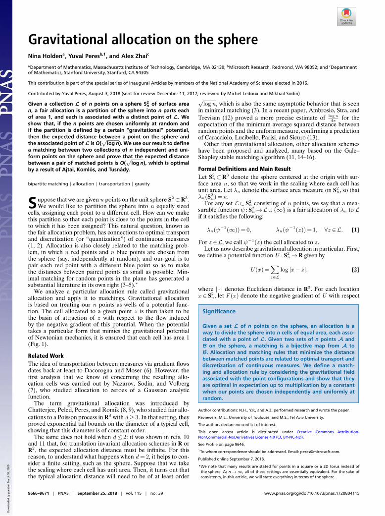
We analyze a particular allocation rule called gravitationalallocation and apply it to matchings. Gravitational allocationis based on treating our n points as wells of a potential func-tion. The cell allocated to a given point z is then taken to bethe basin of attraction of z with respect to the flow inducedby the negative gradient of this potential. When the potentialtakes a particular form that mimics the gravitational potentialof Newtonian mechanics, it is ensured that each cell has area 1(Fig. 1).

Related WorkThe idea of transportation between measures via gradient flowsdates back at least to Dacorogna and Moser (6). However, thefirst analysis that we know of concerning the resulting allo-cation cells was carried out by Nazarov, Sodin, and Volberg(7), who studied allocation to zeroes of a Gaussian analyticfunction.

The term gravitational allocation was introduced byChatterjee, Peled, Peres, and Romik (8, 9), who studied fair allo-cations to a Poisson process in Rd with d ≥ 3. In that setting, theyproved exponential tail bounds on the diameter of a typical cell,showing that this diameter is of constant order.

The same does not hold when d ≤ 2: it was shown in refs. 10and 11 that, for translation invariant allocation schemes in R orR2, the expected allocation distance must be infinite. For thisreason, to understand what happens when d = 2, it helps to con-sider a finite setting, such as the sphere. Suppose that we takethe scaling where each cell has unit area. Then, it turns out thatthe typical allocation distance will need to be of at least order

√log n , which is also the same asymptotic behavior that is seen

in minimal matching (3). In a recent paper, Ambrosio, Stra, andTrevisan (12) proved a more precise estimate of log n

4πfor the

expectation of the minimum average squared distance betweenrandom points and the uniform measure, confirming a predictionof Caracciolo, Lucibello, Parisi, and Sicuro (13).

Other than gravitational allocation, other allocation schemeshave been proposed and analyzed, many based on the Gale–Shapley stable matching algorithm (11, 14–16).

Formal Definitions and Main ResultLet S2

n ⊂R3 denote the sphere centered at the origin with sur-face area n , so that we work in the scaling where each cell hasunit area. Let λn denote the surface area measure on S2

n , so thatλn(S2

n) =n .For any set L⊂S2

n consisting of n points, we say that a mea-surable function ψ : S2

n→L∪{∞} is a fair allocation of λn to Lif it satisfies the following:

λn(ψ−1(∞)) = 0, λn(ψ−1(z )) = 1, ∀z ∈L. [1]

For z ∈L, we call ψ−1(z ) the cell allocated to z .Let us now describe gravitational allocation in particular. First,

we define a potential function U : S2n→R given by

U (x ) =∑z∈L

log |x − z |, [2]

where | · | denotes Euclidean distance in R3. For each locationx ∈S2

n , let F (x ) denote the negative gradient of U with respect

Significance

Given a set L of n points on the sphere, an allocation is away to divide the sphere into n cells of equal area, each asso-ciated with a point of L. Given two sets of n points A andB on the sphere, a matching is a bijective map from A toB. Allocation and matching rules that minimize the distancebetween matched points are related to optimal transport anddiscretization of continuous measures. We define a match-ing and allocation rule by considering the gravitational fieldassociated with the point configurations and show that theyare optimal in expectation up to multiplication by a constantwhen our points are chosen independently and uniformly atrandom.

Author contributions: N.H., Y.P., and A.Z. performed research and wrote the paper.

Reviewers: M.L., University of Toulouse; and M.S., Tel Aviv University.

The authors declare no conflict of interest.

This open access article is distributed under Creative Commons Attribution-NonCommercial-NoDerivatives License 4.0 (CC BY-NC-ND).

See Profile on page 9646.1 To whom correspondence should be addressed. Email: peres@microsoft.com.y

Published online September 7, 2018.

*We note that many results are stated for points in a square or a 2D torus instead ofthe sphere. As n→∞, all of these settings are essentially equivalent. For the sake ofconsistency, in this article, we will state everything in terms of the sphere.

9666–9671 | PNAS | September 25, 2018 | vol. 115 | no. 39 www.pnas.org/cgi/doi/10.1073/pnas.1720804115

Dow

nloa

ded

by g

uest

on

Mar

ch 3

1, 2

020

INA

UG

URA

LA

RTIC

LEA

PPLI

EDM

ATH

EMA

TICS

Fig. 1. Gravitational allocation to n uniform and independent points on asphere with n = 15, 40, 200, and 750. The basin of attraction of each pointhas equal area. The basins become more elongated as n grows, reflectingTheorem 1. The MATLAB script used to generate the gravitational allocationfigures in this article is based on code written by Manjunath Krishnapur.

to the usual spherical metric (i.e., the one induced from R3). Wecan view F (x ) as lying in the plane tangent to S2

n at x (i.e., thetangent space), so that F is a vector field on S2

n .Second, we consider the flow induced by F . For any x ∈S2

n ,let Yx (t) denote the integral curve that solves the differentialequation

dYx

dt(t) =F (Yx (t)), Yx (0) = x . [3]

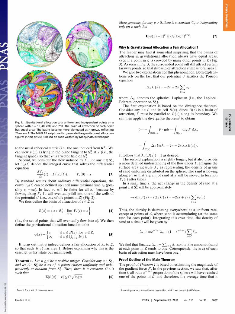
By standard results about ordinary differential equations, thecurve Yx (t) can be defined up until some maximal time τx (pos-sibly τx =∞). In fact, τx will be finite for all x ,† because byflowing along F , Yx will eventually fall into one of the wells ofthe potential U (i.e., one of the points in L) (Fig. 2).

We thus define the basin of attraction of z ∈L as

B(z ) =

{x ∈S2

n : limt↑τx

Yx (t) = z

}[4]

(i.e., the set of points that will eventually flow into z ). We thendefine the gravitational allocation function to be

ψ(x ) =

{z if x ∈B(z ) for z ∈L,∞ if x /∈

⋃z∈L B(z ).

[5]

It turns out that ψ indeed defines a fair allocation of λn to L,so that each B(z ) has area 1. Before explaining why this is thecase, let us first state our main result.

Theorem 1. Let n ≥ 2 be a positive integer. Consider any x ∈S2n ,

and let L⊂S2n be a set of n points chosen uniformly and inde-

pendently at random from S2n . Then, there is a constant C > 0

such thatE|ψ(x )− x | ≤C

√log n. [6]

†Except for a set of measure zero.

More generally, for any p> 0, there is a constant Cp > 0 dependingonly on p such that

E|ψ(x )− x |p ≤Cp(log n)p/2. [7]

Why Is Gravitational Allocation a Fair Allocation?The reader may find it somewhat surprising that the basins ofattraction in gravitational allocation always have equal areas,even if a point in L is crowded by many other points in L (Fig.3). As seen in Fig. 3, the surrounded point will still attract certainfaraway points, so that its basin of attraction still has total area 1.

We give two explanations for this phenomenon. Both explana-tions rely on the fact that our potential U satisfies the Poissonequation

∆SU (x ) =−2π+ 2π∑z∈L

δz ,

where ∆S denotes the spherical Laplacian (i.e., the Laplace–Beltrami operator on S2

n).The first explanation is based on the divergence theorem.

Consider any z ∈L and its cell B(z ). Since B(z ) is a basin ofattraction, F must be parallel to B(z ) along its boundary. Wecan then apply the divergence theorem‡ to obtain

0 =−∫∂B(z)

F · nds =

∫B(z)

divF dλn

=

∫B(z)

∆SUdλn = 2π− 2πλn(B(z )).

It follows that λn(B(z )) = 1 as desired.The second explanation is slightly longer, but it also provides

a more detailed understanding of the flow under F . Imagine thesurface area measure λn as representing the density of grainsof sand uniformly distributed on the sphere. The sand is flowingalong F , so that a grain of sand at x will be moved to locationYx (t) after time t .

In a small time ε, the net change in the density of sand at apoint x ∈S2

n will be approximately

−εdivF (x ) = ε∆SU (x ) =−2πε+ 2πε∑z∈L

δz (x ).

Thus, the density is decreasing everywhere at a uniform rate,except at points of L, where sand is accumulating (at the samerate for each point). Integrating this over time, the density ofsand at a time t will be given by

λn,t : =e−2πtλn + (1− e−2πt)∑z∈L

δz .

We find that limt→∞ λn,t =∑

z∈L δz , so that the amount of sandat each point in L tends to one. Consequently, the area of eachbasin of attraction must have been one.

Proof Outline of the Main TheoremThe proof of Theorem 1 is based on estimating the magnitude ofthe gradient force F . In the previous section, we saw that, aftertime t , all but a e−2πt proportion of the sphere will have reachedone of the points in L, and therefore, the average time that it

‡Assuming various smoothness properties, which we do not justify here.

Holden et al. PNAS | September 25, 2018 | vol. 115 | no. 39 | 9667

Dow

nloa

ded

by g

uest

on

Mar

ch 3

1, 2

020

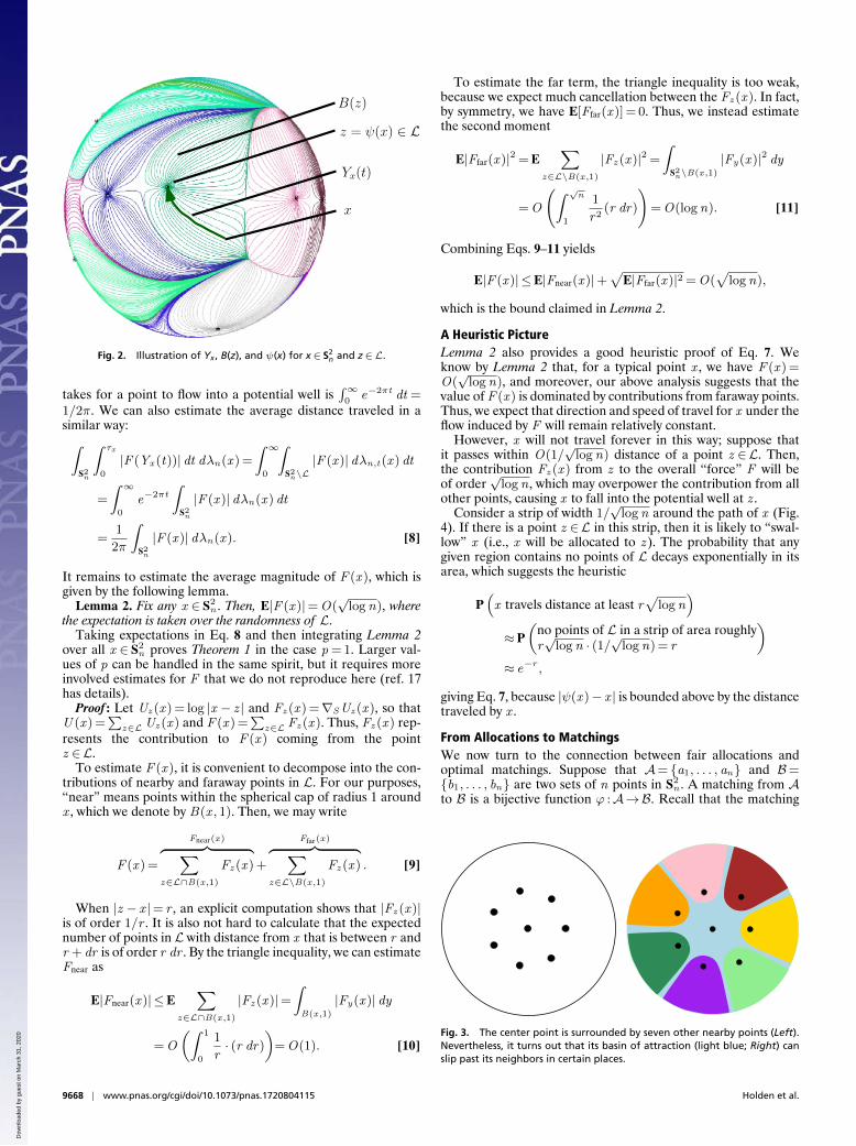
Fig. 2. Illustration of Yx , B(z), and ψ(x) for x∈ S2n and z∈L.

takes for a point to flow into a potential well is∫∞0

e−2πt dt =1/2π. We can also estimate the average distance traveled in asimilar way:∫

S2n

∫ τx

0

|F (Yx (t))| dt dλn(x ) =

∫ ∞0

∫S2n\L

|F (x )| dλn,t(x ) dt

=

∫ ∞0

e−2πt

∫S2n

|F (x )| dλn(x ) dt

=1

2π

∫S2n

|F (x )| dλn(x ). [8]

It remains to estimate the average magnitude of F (x ), which isgiven by the following lemma.

Lemma 2. Fix any x ∈S2n . Then, E|F (x )|=O(

√log n), where

the expectation is taken over the randomness of L.Taking expectations in Eq. 8 and then integrating Lemma 2

over all x ∈S2n proves Theorem 1 in the case p = 1. Larger val-

ues of p can be handled in the same spirit, but it requires moreinvolved estimates for F that we do not reproduce here (ref. 17has details).

Proof : Let Uz (x ) = log |x − z | and Fz (x ) =∇SUz (x ), so thatU (x ) =

∑z∈LUz (x ) and F (x ) =

∑z∈L Fz (x ). Thus, Fz (x ) rep-

resents the contribution to F (x ) coming from the pointz ∈L.

To estimate F (x ), it is convenient to decompose into the con-tributions of nearby and faraway points in L. For our purposes,“near” means points within the spherical cap of radius 1 aroundx , which we denote by B(x , 1). Then, we may write

F (x ) =

Fnear(x)︷ ︸︸ ︷∑z∈L∩B(x ,1)

Fz (x ) +

Ffar(x)︷ ︸︸ ︷∑z∈L\B(x ,1)

Fz (x ) . [9]

When |z − x |= r , an explicit computation shows that |Fz (x )|is of order 1/r . It is also not hard to calculate that the expectednumber of points in L with distance from x that is between r andr + dr is of order r dr . By the triangle inequality, we can estimateFnear as

E|Fnear(x )| ≤E∑

z∈L∩B(x ,1)

|Fz (x )|=∫B(x ,1)

|Fy(x )| dy

=O

(∫ 1

0

1

r· (r dr)

)=O(1). [10]

To estimate the far term, the triangle inequality is too weak,because we expect much cancellation between the Fz (x ). In fact,by symmetry, we have E[Ffar(x )] = 0. Thus, we instead estimatethe second moment

E|Ffar(x )|2 = E∑

z∈L\B(x ,1)

|Fz (x )|2 =

∫S2n\B(x ,1)

|Fy(x )|2 dy

=O

(∫ √n

1

1

r2(r dr)

)=O(log n). [11]

Combining Eqs. 9–11 yields

E|F (x )| ≤E|Fnear(x )|+√

E|Ffar(x )|2 =O(√

log n),

which is the bound claimed in Lemma 2.

A Heuristic PictureLemma 2 also provides a good heuristic proof of Eq. 7. Weknow by Lemma 2 that, for a typical point x , we have F (x ) =O(√

log n), and moreover, our above analysis suggests that thevalue of F (x ) is dominated by contributions from faraway points.Thus, we expect that direction and speed of travel for x under theflow induced by F will remain relatively constant.

However, x will not travel forever in this way; suppose thatit passes within O(1/

√log n) distance of a point z ∈L. Then,

the contribution Fz (x ) from z to the overall “force” F will beof order

√log n , which may overpower the contribution from all

other points, causing x to fall into the potential well at z .Consider a strip of width 1/

√log n around the path of x (Fig.

4). If there is a point z ∈L in this strip, then it is likely to “swal-low” x (i.e., x will be allocated to z ). The probability that anygiven region contains no points of L decays exponentially in itsarea, which suggests the heuristic

P(x travels distance at least r

√log n

)≈P

(no points of L in a strip of area roughlyr√

log n · (1/√

log n) = r

)≈ e−r ,

giving Eq. 7, because |ψ(x )− x | is bounded above by the distancetraveled by x .

From Allocations to MatchingsWe now turn to the connection between fair allocations andoptimal matchings. Suppose that A= {a1, . . . , an} and B={b1, . . . , bn} are two sets of n points in S2

n . A matching from Ato B is a bijective function ϕ :A→B. Recall that the matching

Fig. 3. The center point is surrounded by seven other nearby points (Left).Nevertheless, it turns out that its basin of attraction (light blue; Right) canslip past its neighbors in certain places.

9668 | www.pnas.org/cgi/doi/10.1073/pnas.1720804115 Holden et al.

Dow

nloa

ded

by g

uest

on

Mar

ch 3

1, 2

020

INA

UG

URA

LA

RTIC

LEA

PPLI

EDM

ATH

EMA

TICS

Fig. 4. The speed F is mainly determined by points far away and is approx-imately constant in large regions, except very near points of L. A typicalpoint, therefore, travels in an approximately straight line until it gets withindistance O(1/

√log n) of some point in L.

problem is to find the matching that minimizes the total distancebetween matched points.

When the points of A and B are drawn uniformly at random,the asymptotic behavior of the minimal matching distance wasidentified by Ajtai, Komlos, and Tusnady (3), who proved thefollowing theorem.

Theorem 3 (Ajtai–Komlos–Tusnady). Suppose that A and Beach consist of n points drawn uniformly and independently atrandom from [0,

√n]2. Let

dmatch(A,B) = minϕ:A→Bbijective

1

n

∑a∈A

|ϕ(a)− a|.

Then, there are constants C1,C2> 0 for which

limn→∞

P(C1

√log n ≤ dmatch(A,B)≤C2

√log n

)= 1. [12]

It turns out that the average displacement of a fair alloca-tion gives an upper bound on the matching distance, as the nextproposition shows.

Proposition 4. LetA,B⊂S2n be two sets of n points, and let ψA

and ψB be fair allocations of λn to A and B, respectively. Then,there exists a matching ϕ :A→B such that

∑a∈A

|a −ϕ(a)| ≤∫

S2n

|x −ψA(x )|dλn(x ) +

∫S2n

|x −ψB(x )|dλn(x ).

[13]

Remark 5: Consider the case whereA and B are drawn uniformlyat random, and suppose that we use gravitational allocation forψA and ψB in Proposition 4. Then, the p = 1 case of Theorem1 implies that the right-hand side of Eq. 13 has expectation oforder n

√log n . Comparing with Theorem 3, this implies that the

asymptotic rate of√

log n in Theorem 1 is the best possible up toa constant factor. By Eq. 8, we also get that E|F (x )| is at least oforder

√log n for any fixed x ∈S2

n .The triangle inequality for the linear Wasserstein distance jus-

tifies why we can pass from an allocation to a matching, but wechoose to describe the connection explicitly. Let Ai =ψ−1

A (ai)

denote the cell allocated to ai , and similarly, let Bi =ψ−1B (bi).

Consider the n ×n matrix M = (Mij )ni,j=1 given by

Mij =λn(Ai ∩Bj ).

We see that M is a doubly stochastic matrix:

n∑j=1

Mij =

n∑j=1

λn(Ai ∩Bj ) =λn(Ai) = 1,

n∑i=1

Mij =

n∑i=1

λn(Ai ∩Bj ) =λn(Bj ) = 1.

By the Birkhoff–von Neumann theorem (ref. 18, theorem 5.5),any doubly stochastic matrix is a convex combination of permu-tation matrices. For a permutation σ, we write Pσ to denote thecorresponding permutation matrix, so that Pσij = 1 if j =σ(i) andPσij = 0 otherwise. Then, we may write

M =

N∑k=1

ckPσk , [14]

where ck are nonnegative numbers summing to one and σk arepermutations.

Let X be chosen uniformly at random from S2n . Observe

that nP[X ∈Ai ∩Bj ] =Mij and that |ψA(X )−ψB(X )|= |ai −bj | on the event X ∈Ai ∩Bj . By Eq. 14 and this observation,

minσ

n∑i=1

n∑j=1

Pσij |ai − bj | ≤n∑

i=1

n∑j=1

Mij |ai − bj |

=nE|ψA(X )−ψB(X )|. [15]

By the triangle inequality, the right side of Eq. 15 is boundedabove by the right side of Eq. 13, which implies Proposition 4.

Online MatchingOne can also consider an “online” version of the matching prob-lem, in which we initially see only the points in B, and we aregiven the points inA= {a1, a2, . . . , an} one by one. As soon as aiis revealed to us, we must immediately match it to a point ϕ(ai)in B (that has not already been matched). In particular, we makethis decision without knowing the locations of the remainingpoints in A.

There is a natural online matching algorithm using gravita-tional allocation. When a point ak is revealed, let B′ be the setof points in B that have not yet been matched. We then considerthe gravitational allocation ψB′ to B′ and match ak to ψB′(ak ).

The analysis of this procedure is particularly simple if thepoints of A and B are sampled uniformly and independently atrandom. Consider what happens when we pair the first point a1.According to Theorem 1, the expected distance between a1 andits pair is bounded by

E|a1−ϕ(a1)|= E|a1−ψB(a1)| ≤C√

log n.

Since ψB gives a fair allocation and the first point a1 is drawnuniformly at random, each of the points in B is an equally likelymatch for a1 under our scheme. It follows that the remainingpoints B \ {ϕ(a1)} will still be distributed uniformly and inde-pendently at random. Thus, we have reduced the problem tomatching two sets of n − 1 independent random points on S2

n

after incurring a cost of C√

log n for matching the first pair(Fig. 5).

We may iterate this analysis for each point in A. When wereceive ak , there will be m : =n − k + 1 remaining unpairedpoints in B (still uniformly distributed), so that a typical distance

Fig. 5. Illustration of the online matching algorithm. The set B \ϕ(a1)consists of n− 1 uniform and independent points on the sphere S2

n ofarea n.

Holden et al. PNAS | September 25, 2018 | vol. 115 | no. 39 | 9669

Dow

nloa

ded

by g

uest

on

Mar

ch 3

1, 2

020

in gravitational allocation will be O(√

n/m · logm), where the

factor√

n/m comes from rescaling S2m to S2

n . Thus,

n∑k=1

E|ak −ϕ(ak )| ≤n∑

m=2

O(√

n/m · logm)

≤O(√

n log n)

n∑m=2

1√m

=O(n√

log n),

which shows that, even in the online setting, one has similarasymptotics as in Theorem 3.

We remark that our online matching algorithm can be imple-mented efficiently using the well-known “fast multipole method”introduced by Rokhlin (19) and Greengard and Rokhlin (20).This entails precomputing estimates of the gravitational poten-tial from clusters of points in B, and these computations can bereused as new points of A are introduced.

Gravitational Allocation for Other Point ProcessesSo far, we have focused on the setting where our n points onS2n are taken independently at random. However, one may also

analyze other random point processes where the points are notindependent, which allows them to be distributed more evenlyover the sphere.

One example is given by the roots of a certain Gaussianrandom polynomial. Specifically, we look at the polynomial

p(z ) =

n∑k=0

ζk

√n(n − 1) · · · (n − k + 1)√

k !z k ,

where ζ1, . . . , ζn are independent standard complex Gaussians.The roots λ1, . . . ,λn of p are then n random points in the com-plex plane, which we can bring to the sphere via stereographicprojection. More explicitly, let x0 = (0, 0, 1). The function

P : z 7→√

n

4π

(x0 +

2(z − x0)

|z − x0|2

)maps the horizontal plane in R3 to S2

n . Then, viewing the λk aslying in the horizontal plane,

L= {P(λk )}nk=1

is a rotationally equivariant random set of n points on S2n .

[The rotational equivariance comes from the particular choiceof coefficients for p (ref. 21, chapter 2.3).]

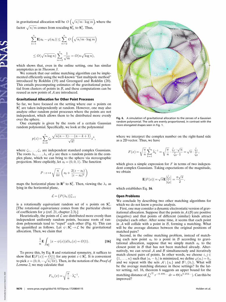
Heuristically, the points of L are distributed more evenly thanindependent uniformly random points, because roots of ran-dom polynomials tend to “repel” each other (Fig. 6). This canbe quantified as follows. Let ψ : S2

n→L be the gravitationalallocation. Then, we claim that

1

nE∫

S2n

|x −ψ(x )|dλn(x ) =O(1). [16]

To prove this, by Eq. 8 and rotational symmetry, it suffices toshow that E|F (x )|=O(1) for any point x ∈S2

n . It is convenientto pick x = (0, 0,−

√n/4π). Then, in the notation of the Proof of

Lemma 2, we may calculate that

Fλk (x ) =

√π

n· λ−1

k ,

Fig. 6. A simulation of gravitational allocation to the zeroes of a Gaussianrandom polynomial. The cells are evenly proportioned, in contrast with themore elongated shapes seen in Fig. 1.

where we interpret the complex number on the right-hand sideas a 2D vector. Thus, we have

F (x ) =

√π

n

n∑k=1

λ−1k =

√π

n· ζ1 ·

√n

ζ0 · 1=√π · ζ1

ζ0,

which gives a simple expression for F in terms of two indepen-dent complex Gaussians. Taking expectations of the magnitude,we obtain

E|F (x )|=√πE|ζ1||ζ0|

=π√π

2,

which establishes Eq. 16.

Open ProblemsWe conclude by describing two other matching algorithms forwhich we do not know a precise analysis.

First, one may consider a dynamic electrostatic version of grav-itational allocation. Suppose that the points inA (B) are positive(negative) and that points of different (similar) kinds attract(repulse) each other. After some time, it seems that each pointin A will collide with a point in B, forming a matching. Whatwill be the average distance between the original positions ofmatched pairs?

Second, in the online matching problem, instead of match-ing each new point ak to a point in B according to gravi-tational allocation, suppose that we simply match ak to theclosest point in B that has not been matched already. Alter-natively, we can reveal A and B simultaneously and iterativelymatch closest pairs of points. In other words, we choose i , j ∈{1, . . . ,n} such that |ai − bj | is minimized, we define ϕ(ai) = bj ,and we repeat with the sets A\{ai} and B \ {bj}. What willbe the average matching distance in these settings? In the lat-ter setting, ref. 16, theorem 6 suggests an upper bound for thematching distance of

∫√n

0r−0.496... dr = Θ(n0.252...). Can this be

improved?

9670 | www.pnas.org/cgi/doi/10.1073/pnas.1720804115 Holden et al.

Dow

nloa

ded

by g

uest

on

Mar

ch 3

1, 2

020

INA

UG

URA

LA

RTIC

LEA

PPLI

EDM

ATH

EMA

TICS

ACKNOWLEDGMENTS. We thank Manjunath Krishnapur for useful discus-sions as well as for sharing his code for producing simulations. Most of this

work was carried out while N.H. and A.Z. were visiting Microsoft Research;we thank Microsoft Research for the hospitality.

1. Huesmann M, Sturm KT (2013) Optimal transport from Lebesgue to Poisson. AnnProbab 41:2426–2478.

2. Dereich S, Scheutzow M, Schottstedt R (2013) Constructive quantization: Approxima-tion by empirical measures. Ann Inst Henri Poincare Probab Stat 49:1183–1203.

3. Ajtai M, Komlos J, Tusnady G (1984) On optimal matchings. Combinatorica 4:259–264.

4. Leighton T, Shor P (1989) Tight bounds for minimax grid matching with applicationsto the average case analysis of algorithms. Combinatorica 9:161–187.

5. Talagrand M (1994) Matching theorems and empirical discrepancy computationsusing majorizing measures. J Am Math Soc 7:455–537.

6. Dacorogna B, Moser J (1990) On a partial differential equation involving the Jacobiandeterminant. Ann de l’Institut Henri Poincare Analyse Non Lineaire 7:1–26.

7. Nazarov F, Sodin M, Volberg A (2007) Transportation to random zeroes by thegradient flow. Geom Funct Anal 17:887–935.

8. Chatterjee S, Peled R, Peres Y, Romik D (2010) Gravitational allocation to Poissonpoints. Ann Math 172:617–671.

9. Chatterjee S, Peled R, Peres Y, Romik D (2010) Phase transitions in gravitationalallocation. Geom Funct Anal 20:870–917.

10. Holroyd AE, Liggett TM (2001) How to find an extra head: Optimal random shifts ofBernoulli and Poisson random fields. Ann Probab 29:1405–1425.

11. Hoffman C, Holroyd AE, Peres Y (2006) A stable marriage of Poisson and Lebesgue.Ann Probab 34:1241–1272.

12. Ambrosio L, Stra F, Trevisan D (2018) A PDE approach to a 2-dimensional match-ing problem. Probab Theory Relat Fields. Available at https://link.springer.com/article/10.1007%2Fs00440-018-0837-x#citeas. Accessed September 4, 2018.

13. Caracciolo S, Lucibello C, Parisi G, Sicuro G (2014) Scaling hypothesis for the Euclideanbipartite matching problem. Phys Rev E 90:012118.

14. Holroyd AE, Peres Y (2005) Extra heads and invariant allocations. Ann Probab 33:31–52.

15. Hoffman C, Holroyd AE, Peres Y (2009) Tail bounds for the stable marriage of Poissonand Lebesgue. Canad J Math 61:1279–1299.

16. Holroyd AE, Pemantle R, Peres Y, Schramm O (2009) Poisson matching. Ann Inst HenriPoincare Probab Stat 45:266–287.

17. Holden N, Peres Y, Zhai A (2017) Gravitational allocation for uniform points on thesphere. arXiv:170408238. Preprint, posted April 26, 2017.

18. van Lint JH, Wilson RM (2001) A Course in Combinatorics (Cambridge Univ Press,Cambridge, UK), 2nd Ed.

19. Rokhlin V (1985) Rapid solution of integral equations of classical potential theory. JComput Phys 60:187–207.

20. Greengard L, Rokhlin V (1987) A fast algorithm for particle simulations. J ComputPhys 73:325–348.

21. Hough JB, Krishnapur M, Peres Y, Virag B (2009) Zeros of Gaussian Analytic Functionsand Determinantal Point Processes, University Lecture Series (American MathematicalSociety, Providence, RI), Vol 51.

Holden et al. PNAS | September 25, 2018 | vol. 115 | no. 39 | 9671

Dow

nloa

ded

by g

uest

on

Mar

ch 3

1, 2

020