grizzly/favor interface project report
TRANSCRIPT
ORNL/TM-2013/44094
Grizzly/FAVOR Interface
Project Report
Prepared by T.L. Dickson, P.T. Williams, S. Yin, H.B. Klasky, S. K. Tadinada, B.R. Bass Oak Ridge National Laboratory Prepared for J.T. Busby and B.D. Wirth Light Water Reactor Sustainability Program Risk-Informed Safety Margin Characterization

DOCUMENT AVAILABILITY Reports produced after January 1, 1996, are generally available free via the U.S. Department of Energy (DOE) Information Bridge. Web site http://www.osti.gov/bridge Reports produced before January 1, 1996, may be purchased by members of the public from the following source. National Technical Information Service 5285 Port Royal Road Springfield, VA 22161 Telephone 703-605-6000 (1-800-553-6847) TDD 703-487-4639 Fax 703-605-6900 E-mail [email protected] Web site http://www.ntis.gov/support/ordernowabout.htm Reports are available to DOE employees, DOE contractors, Energy Technology Data Exchange (ETDE) representatives, and International Nuclear Information System (INIS) representatives from the following source. Office of Scientific and Technical Information P.O. Box 62 Oak Ridge, TN 37831 Telephone 865-576-8401 Fax 865-576-5728 E-mail [email protected] Web site http://www.osti.gov/contact.html
This report was prepared as an account of work sponsored by an agency of the United States Government. Neither the United States Government nor any agency thereof, nor any of their employees, makes any warranty, express or implied, or assumes any legal liability or responsibility for the accuracy, completeness, or usefulness of any information, apparatus, product, or process disclosed, or represents that its use would not infringe privately owned rights. Reference herein to any specific commercial product, process, or service by trade name, trademark, manufacturer, or otherwise, does not necessarily constitute or imply its endorsement, recommendation, or favoring by the United States Government or any agency thereof. The views and opinions of authors expressed herein do not necessarily state or reflect those of the United States Government or any agency thereof.

ORNL/TM-2013/44094
Grizzly/FAVOR Interface
Project Report
Manuscript Completed: June 2013 Date Published: June 2013
Authors: T.L. Dickson, P.T. Williams, S. Yin, H.B. Klasky, S. Tadinada, B.R. Bass Prepared for J. T. Busby and B. D. Wirth Light Water Reactor Sustainability Program Risk-Informed Safety Margin Characterization
Prepared by OAK RIDGE NATIONAL LABORATORY
Oak Ridge, Tennessee 37831-6085 managed by
UT-BATTELLE, LLC for the
U.S. DEPARTMENT OF ENERGY

ii
This page is intentionally left blank.

iii
ABSTRACT
As part of the Light Water Reactor Sustainability (LWRS) Program, the objective of the Grizzly/FAVOR Interface project is to create the capability to apply Grizzly 3-D finite element (thermal and stress) analysis results as input to FAVOR probabilistic fracture mechanics (PFM) analyses. The one benefit of FAVOR to Grizzly is the PROBABILISTIC capability. This document describes the implementation of the Grizzly/FAVOR Interface, the preliminary verification and tests results and a user guide that provides detailed step-by-step instructions to run the program.

iv
CONTENTS Page
ABSTRACT .. . . . . . . . . . . . . . . . . . . . . . . . . . . . . . . . . . . . . . . . . . . . . . . . . . . . . . . . . . . . . . . . . . . . . . . . . . . . . . . . . . . . . . . . . . . . . . . . . . . i i i CONTENTS . . . . . . . . . . . . . . . . . . . . . . . . . . . . . . . . . . . . . . . . . . . . . . . . . . . . . . . . . . . . . . . . . . . . . . . . . . . . . . . . . . . . . . . . . . . . . . . . . . . . iv LIST OF FIGURES . . . . . . . . . . . . . . . . . . . . . . . . . . . . . . . . . . . . . . . . . . . . . . . . . . . . . . . . . . . . . . . . . . . . . . . . . . . . . . . . . . . . . . . . . . v LIST OF TABLES . . . . . . . . . . . . . . . . . . . . . . . . . . . . . . . . . . . . . . . . . . . . . . . . . . . . . . . . . . . . . . . . . . . . . . . . . . . . . . . . . . . . . . . . . . vii ABBREVIATIONS . . . . . . . . . . . . . . . . . . . . . . . . . . . . . . . . . . . . . . . . . . . . . . . . . . . . . . . . . . . . . . . . . . . . . . . . . . . . . . . . . . . . . . . . vii i 1. INTRODUCTION .. . . . . . . . . . . . . . . . . . . . . . . . . . . . . . . . . . . . . . . . . . . . . . . . . . . . . . . . . . . . . . . . . . . . . . . . . . . . . . . . . . . . . . 1
1.1 LWRS Overview . . . . . . . . . . . . . . . . . . . . . . . . . . . . . . . . . . . . . . . . . . . . . . . . . . . . . . . . . . . . . . . . . . . . . . . . . . . . . . . . . . . . 1 1.2 Grizzly Overview . . . . . . . . . . . . . . . . . . . . . . . . . . . . . . . . . . . . . . . . . . . . . . . . . . . . . . . . . . . . . . . . . . . . . . . . . . . . . . . . . . 1 1.3 FAVOR Overview . . . . . . . . . . . . . . . . . . . . . . . . . . . . . . . . . . . . . . . . . . . . . . . . . . . . . . . . . . . . . . . . . . . . . . . . . . . . . . . . . . 2 1.4 GRIZZLY/FAVOR Interface Overview . . . . . . . . . . . . . . . . . . . . . . . . . . . . . . . . . . . . . . . . . . . . . . . . . . 2
2. Grizzly/FAVOR INTERFACE IMPLEMENTATION .. . . . . . . . . . . . . . . . . . . . . . . . . . . . . . . . . . . 3 2.1 FAVOR – Computational Modules and Data Streams . . . . . . . . . . . . . . . . . . . . . . . . . . . . . 3 2.2 The Grizzly/FAVOR Interface . . . . . . . . . . . . . . . . . . . . . . . . . . . . . . . . . . . . . . . . . . . . . . . . . . . . . . . . . . . . . . . 5 2.3 Grizzly/FAVOR Interface Input Description . . . . . . . . . . . . . . . . . . . . . . . . . . . . . . . . . . . . . . . . . . 6 2.4 Grizzly/FAVOR Interface Output Files . . . . . . . . . . . . . . . . . . . . . . . . . . . . . . . . . . . . . . . . . . . . . . . . 17 2.5 Grizzly/FAVOR Interface Software Engineering Metrics . . . . . . . . . . . . . . . . . . . . . 20
3. VERIFICATION .. . . . . . . . . . . . . . . . . . . . . . . . . . . . . . . . . . . . . . . . . . . . . . . . . . . . . . . . . . . . . . . . . . . . . . . . . . . . . . . . . . . . . 21 3.1 Initial Benchmarking of FAVOR and Grizzly . . . . . . . . . . . . . . . . . . . . . . . . . . . . . . . . . . . . . . . 21 3.2 Initial Testing of the Grizzly –FAVOR Interface . . . . . . . . . . . . . . . . . . . . . . . . . . . . . . . . . 27
4. Grizzly/FAVOR INTERFACE USER GUIDE .. . . . . . . . . . . . . . . . . . . . . . . . . . . . . . . . . . . . . . . . . . . . 35 4.1 Grizzly/FAVOR Interface Distribution . . . . . . . . . . . . . . . . . . . . . . . . . . . . . . . . . . . . . . . . . . . . . . . . 35 4.2 Hardware and SOFTWARE Requirements . . . . . . . . . . . . . . . . . . . . . . . . . . . . . . . . . . . . . . . . . . . 35 4.3 Running the Grizzly/FAVOR Interface . . . . . . . . . . . . . . . . . . . . . . . . . . . . . . . . . . . . . . . . . . . . . . . . 37 4.4 Contacts . . . . . . . . . . . . . . . . . . . . . . . . . . . . . . . . . . . . . . . . . . . . . . . . . . . . . . . . . . . . . . . . . . . . . . . . . . . . . . . . . . . . . . . . . . . . . . 45
5. CONCLUSIONS AND FUTURE SUGGESTIONS . . . . . . . . . . . . . . . . . . . . . . . . . . . . . . . . . . . . . . . 46 6. REFERENCES . . . . . . . . . . . . . . . . . . . . . . . . . . . . . . . . . . . . . . . . . . . . . . . . . . . . . . . . . . . . . . . . . . . . . . . . . . . . . . . . . . . . . . . . . 47

v
LIST OF FIGURES
Figure Page Figure 1. FAVOR data streams flow through three modules: (1) FAVLoad, (2) FAVPFM, and (3) FAVPost. ....................................................................................................................... 3 Figure 2. The FAVOR load generator module FAVLoad performs deterministic analyses for a range of thermal-hydraulic transients. .................................................................................... 4 Figure 3. The FAVPFM module takes output from FAVLoad and user-supplied data on flaw distributions and embrittlement of the RPV beltline and generates PFMI and PFMF arrays. .. 5 Figure 4. Implementation of the Grizzly/FAVOR interface. ..................................................... 6 Figure 5 Beaver Valley transient sequence 130 thermal hydraulic boundary condition - sever re-pressurization- is a dominant transient generated by RELAP5. ......................................... 22 Figure 6 Probability distribution function for the transient frequency for Beaver Valley transient sequence 130. ............................................................................................................ 23 Figure 7 Mutual verification of temperature time history solutions at point in wall thickness for Beaver Valley transient sequence 130. .............................................................................. 24 Figure 8 Mutual verification of axial stress time history solutions at point in wall thickness for Beaver Valley transient sequence 130. .............................................................................. 25 Figure 9 Mutual verification of hoop stress time history solutions at point in wall thickness for Beaver Valley transient sequence 130. .............................................................................. 26 Figure 10 Illustration of Beaver Valley transient sequence 007 - a severe cooldown transient caused by surge line break. ...................................................................................................... 28 Figure 11 Verification of Grizzly-FAVOR interface for temperature - time history at various locations thru-the-wall thickness ............................................................................................. 29 Figure 12 Verification of Grizzly-FAVOR interface for axial stress - time history at various locations thru-the-wall thickness ............................................................................................. 30 Figure 13 Verification of Grizzly-FAVOR interface for hoop stress-time history at various locations thru-the-wall thickness. ............................................................................................ 31 Figure 14 Verification of Grizzly-FAVOR interface for spatial profiles of thru-wall temperatures at different transient times. ................................................................................ 32 Figure 15 Verification of Grizzly-FAVOR interface for spatial profiles of thru-wall axial stress at different transient times ............................................................................................. 33 Figure 16 Verification of Grizzly-FAVOR interface for spatial profiles of thru-wall hoop stress at different transient times. ............................................................................................ 34 Figure 17. Execution of the Grizzly/FAVOR interface module: (a) type in FAVOR_Grizzly_interface.exe at the line prompt and (b) respond to prompts for the input and output file names ............................................................................................................... 39 Figure 18. The Grizzly/FAVOR interface calculates thermal, stress, and applied KI loading for all of the transients defined in the input file. ..................................................................... 40 Figure 19. Type FAVPFM.EXE at the Command Prompt to begin execution of the FAVPFM module. .................................................................................................................................... 41 Figure 20. FAVPFM prompts for the names of the (1) FAVPFM input file, (2) FAVLoad-generated load-definition file, (3) FAVPFM output file, (4) flaw-characterization file for

vi
surface-breaking flaws in welds and plates, (5) flaw-characterization file for embedded flaws in welds, and (6) flaw-characterization file for embedded flaws in plates. ............................. 42 Figure 21. FAVPFM continually writes out progress reports in terms of running average CPI/CPF values for each transient as the code proceeds through the required number of RPV trials. ........................................................................................................................................ 43 Figure 22. Type in FAVPost at the Command Prompt to execute the FAVPost module. FAVPost prompts for the (1) FAVPost input file, (2) CPI matrix file generated by FAVPFM, (3) CPF matrix file generated by FAVPFM, and (4) the FAVPost output file. Set the total number of simulations to be processed and build convergence tables, if required. ................ 44

vii
LIST OF TABLES Table Page Table 1 Record Keywords and Parameter Fields for FAVLoad Input File ............................... 8

viii
ABBREVIATIONS FAVOR Fracture Analysis of Vessels – Oak Ridge Grizzly A MOOSE-based tool for simulating component ageing and damage evolution events
for LWRS specific applications. INL Idaho National Laboratory JFNK Jacobian-Free Newton Krylov LEFM Linear-Elastic Fracture Mechanics LWRS Light Water Reactor Sustainability Program MOOSE Multi-Physics Object-Oriented Simulation Environment NNSA National Nuclear Security Administration ORNL Oak Ridge National Laboratory PETSc Portable, Extensible Toolkit for Scientific Computation Project PDF Probability Distribution Function PFM Probabilistic Fracture Mechanics PTS Pressurized Thermal Shock RELAP5 Reactor Excursion and Leak Analysis Program 5. RPV Reactor Pressure Vessel SAPHIRE7 Systems Analysis Programs for Hands-on Integrated Reliability Evaluation Version
7. SIFIC Stress-Intensity Influence Coefficient Factor

ix


1
1. INTRODUCTION
This chapter presents overviews of the LWRS Program, Grizzly, FAVOR, and the Grizzly/FAVOR interface. It also emphasizes the benefits to Grizzly from FAVOR: the main benefit of FAVOR to Grizzly is the PROBABILISTIC capability.
1.1 LWRS Overview
The Light Water Reactor Sustainability (LWRS) Program [3] is designed to support the long-term operation (LTO) of existing domestic nuclear power generation with targeted collaborative research programs into areas beyond current short-term optimization opportunities. The LWRS Program focuses on four main areas: Materials Aging and Degradation, Advanced Instrumentation, Information, and Control Systems Technologies, Advanced Light Water Reactor Nuclear Fuels, and finally, Risk-Informed Safety Margin Characterization.
The Materials Aging and Degradation Pathway goal is to develop the scientific basis for understanding and predicting long-term environmental degradation behavior of materials in nuclear power plants and to provide data and methods to assess performance of systems, structures, and components essential to safe and sustained nuclear power plant operations.
The purpose of the Risk-Informed Safety Margin Characterization Pathway is to develop and deploy approaches to support the management of uncertainty in safety margins quantification to improve decision making for nuclear power plants. Management of uncertainty implies the ability to (a) understand and (b) control risks related to safety. Consequently, the RISMC Pathway is dedicated to improving both aspects of safety management.
1.2 Grizzly Overview
Grizzly [4] is a MOOSE-based tool for simulating component ageing and damage evolution events for LWRS specific applications. The Multi-physics Object Oriented Simulation Environment (MOOSE) is the Idaho National Laboratory’s (INL) development and runtime environment for the solution of multi-physics systems that involve multiple physical models or multiple simultaneous physical phenomena. The systems are generally represented (modeled) as a system of fully coupled nonlinear partial differential equation systems (an example of a multi-physics system is the thermal feedback effect upon neutronics cross-sections where the cross-sections are a function of the heat transfer). Inside MOOSE, the Jacobian-Free Newton Krylov (JFNK) method is implemented as a parallel nonlinear solver that naturally supports effective coupling between physics equation systems (or Kernels). The physics Kernels are designed to contribute to the nonlinear residual, which is then minimized inside of MOOSE. MOOSE provides a comprehensive set of finite element support capabilities (libMesh) and provides for mesh adaptation and parallel execution. The framework heavily leverages software libraries from the U.S. Department of Energy Office of Science (DOE SC) and the National Nuclear Security Administration (NNSA), such as the nonlinear solver capabilities in either the Portable, Extensible Toolkit for Scientific Computation (PETSc) project or the Trilinos project.
Specifically, Grizzly will provide a simulation capability for: • Reactor Metals (embrittlement, fatigue, corrosion, etc.), such as Reactor Pressure Vessel
(RPV) and core internals • Weldment integrity • Concrete integrity

2
subjected to a neutron flux, corrosive environment, and high temperatures and pressures. As with other applications utilizing the ever-growing library of MOOSE physics Kernels, Grizzly will heavily leverage the thermo-mechanics physics found in the BISON fuels performance application as a starting point.
1.3 FAVOR Overview
The Fracture Analysis of Vessels – Oak Ridge (FAVOR) computer code [1, 2] was developed and it is being maintained at Oak Ridge National Laboratory (ORNL) for the NRC. FAVOR includes implementations of significant advancements and refinements in technologies that have impacted established fracture mechanics and risk-informed methodologies. Updated computational methodologies have been developed through interactions between experts in the relevant disciplines of thermal hydraulics, probabilistic risk assessment, materials embrittlement, fracture mechanics, and inspection (flaw characterization). These methodologies have been and continue to be applied in the assessment and updating of regulations designed to insure that the structural integrity of aging and increasingly radiation-embrittled nuclear reactor pressure vessels (RPVs) is maintained throughout the licensing period of the reactor.
Contributors to the development of these methodologies include the U.S. Nuclear Regulatory Commission (NRC) staff, their contractors, and representatives from the nuclear industry. The analysis of Pressurized Thermal Shock (PTS) transients in nuclear power plants was the primary motivation for the initial development of FAVOR; earlier versions of FAVOR were limited to performing fracture analyses of pressurized water reactors (PWRs) subjected to cool-down transients.
On January 2013, the 12.1 version of FAVOR was deployed. FAVOR V. 12.1 represents a significant generalization over previous versions, because the problem class for FAVOR has been extended to encompass a broader range of events that include normal operational transients (start-up, shut-down, and leak-test) as well as upset conditions such as PTS. This latest version of FAVOR provides the capability to perform deterministic and risk-informed probabilistic fracture analyses of boiling water reactors (BWRs) and PWRs subjected to heat-up and / or cool-down transients.
The FAVOR computer code continues to evolve and to be extensively applied by analysts from the nuclear industry and regulators at the NRC to insure that the structural integrity of aging and increasingly radiation-embrittled nuclear reactor pressure vessels (RPVs) is maintained through-out the licensing period of the reactor. The FAVOR, v12.1, code represents the latest NRC-selected applications tool for performing such analyses.
FAVOR has extensive capability for calculation of applied KI for a wide variety of postulated defects – as required for fracture analysis. FAVOR PFM methodology is accepted by United States Nuclear Regulatory Commission and has been used in updates of RPV regulations regarding re-licensing of reactors from 40 to 60 years.
1.4 GRIZZLY/FAVOR Interface Overview
The objective of the Grizzly/FAVOR interface project is to create the capability to apply Grizzly 3-D finite element (thermal and stress) analysis results as input to FAVOR probabilistic fracture mechanics (PFM) analyses. The latter objective has been implemented by mapping the Grizzly output to the format required by the current FAVPFM module in FAVOR; from here, the execution flow of FAVOR remains unmodified. The main benefit of FAVOR to Grizzly is the PROBABILISTIC capability to calculate failures for structures.
In the following section, the Grizzly/FAVOR interface is described in detail.

3
2. Grizzly/FAVOR INTERFACE IMPLEMENTATION
This section presents the implementation of the Grizzly/FAVOR interface.
2.1 FAVOR – Computational Modules and Data Streams
As presented in Figure 1, FAVOR is composed of three computational modules: (1) a deterministic load generator (FAVLoad), (2) a Monte Carlo PFM module (FAVPFM), and (3) a post-processor (FAVPost). Figure 1 also indicates the nature of the data streams that flow through these modules. The formats of the required user-input data files are discussed in detail in the FAVOR, v12.1: User’s Guide [2].
Figure 1. FAVOR data streams flow through three modules: (1) FAVLoad, (2) FAVPFM, and
(3) FAVPost.

4
The functional structure of the FAVOR load module, FAVLoad, is shown in Figure 2, where multiple thermal-hydraulic transients are defined in the input data. The number of transients that can be analyzed in a single execution of FAVLoad is dependent upon the memory capacity of the computer being used for the analysis. For each transient, deterministic calculations are performed to produce a load-definition input file for FAVPFM. These load-definition files include time-dependent through-wall temperature profiles, through-wall circumferential and axial stress profiles, and stress-intensity factors (SIFs) for a range of axially- and circumferentially-oriented inner and external surface-breaking flaw geometries (both infinite- and finite-length).
Figure 2. The FAVOR load generator module FAVLoad performs deterministic analyses for a
range of thermal-hydraulic transients.
As shown in Figure 3, the FAVPFM module requires, as input, load-definition data from FAVLoad and user-supplied data on flaw distributions and embrittlement of the RPV beltline. FAVPFM then generates two matrices: (1) the conditional probability of crack initiation (PFMI) matrix and (2) conditional probability of through-wall cracking (PFMF) matrix. The (i, j)th entry in each array contains the results of the PFM analysis for the jth vessel simulation subjected to the ith transient.

5
Figure 3. The FAVPFM module takes output from FAVLoad and user-supplied data on flaw
distributions and embrittlement of the RPV beltline and generates PFMI and PFMF arrays.
2.2 The Grizzly/FAVOR Interface
The Grizzly/FAVOR interface has been implemented in the FAVLoad module described above.
The linear-elastic fracture mechanics (LEFM) methodologies applied in FAVOR require as input the stress-state and temperature fields for an unflawed structure. Using linear superposition, stress-intensity influence coefficients (SIFICs) (stored in a library in FAVLoad) combined with the stress-state of an unflawed structure allow the determination of stress-intensity factors which contribute to the characterization of the driving forces on a postulated crack in a probabilistic assessment of the structural reliability of the RPV.
For the cracked structure under LEFM conditions, the singular stress field in the vicinity of the crack tip can be characterized by a single parameter. This one-parameter model has the form
hoop stresses for axial flaws
2
axial stresses for circumferential flaws2
θθσπ
σπ
=
=
I
Izz
Kr
Kr
(1)
where r is the radial distance from the crack tip, and the crack plane is assumed to be a principal plane. The critical fracture parameter in Eq. (1) is the Mode I stress-intensity factor, KI. When the conditions for LEFM are met, the problem of calculating the stress-intensity factor can be formulated solely in terms of the flaw geometry and the stress distribution of the uncracked structure.
In linking the Grizzly and FAVOR applications, it is intended to replace the 1-D stress and temperature fields calculated by the FAVLoad module with the fully 3-D solutions obtained by Grizzly. These 3-D stresses from Grizzly will serve as input to the Grizzly/FAVOR interface. The Grizzly/FAVOR interface performs the mapping and conversion of the Grizzly output to comply with

6
FAVOR’s FAVPFM module input format for its load definition file. From this step on, the flow and execution of FAVOR remains un-modified. The required modifications to FAVOR occur only in the FAVLoad module; therefore, the resulting Grizzly/FAVOR interface replaces the FAVLoad module as shown in Figure 4.
Figure 4. Implementation of the Grizzly/FAVOR interface.
2.3 Grizzly/FAVOR Interface Input Description
The FAVOR_Grizzly interface requires as input a single ASCII text file. In the following section, we present extracts of an input dataset for the FAVOR_Grizzly interface. As an example, the input file could be named FAVLoad1_GRI.in. As a proof of principle, this initial prototype will consider only one thermal-hydraulic transient.

7
Note that the Grizzly mesh, temperature, axial stress, and hoop stresses are appended onto an existing FAVLoad input dataset. This format minimizes the number of modifications that have to be made to FAVLoad. The Grizzly/FAVLoad module reads in the Grizzly solutions (mesh, temps, and stresses) and maps them (by piecewise cubic spline fits) to locations that FAVLoad then uses in the calculation of KI values.
A total of 20 data records, listed in Table 1, are required in the Grizzly/FAVLoad input file, where each record may involve more than one line of data. A detailed description of each data record is given below.

8
Table 1 Record Keywords and Parameter Fields for FAVLoad Input File 1 GEOM IRAD=[in] W=[in] CLTH=[in]2 BASE K=[Btu/hr-ft-°F] C=[Btu/lbm-°F]RHO=[lbm/ft3] E=[ksi] ALPHA=[°F -1] NU=[-] NTE=[0|1]2a NBK NK=[-] if NTE=1
input NK data lines with {T, K(T) } [°F, Btu/h-ft-°F] pairs - one pair per line2b NBC NC=[-] if NTE=1
input NC data lines with {T, C(T) } [°F, Btu/lbm-°F] pairs - one pair per line2c NBE NE=[-] if NTE=1
input NE data lines with {T, E(T) } [°F, ksi] pairs - one pair per line2d NALF NA=[-] Tref0=[°F] if NTE=1
input NA data lines with {T, ALPHA(T) } [°F, °F -1] pairs - one pair per line2e NNU NU=[-] if NTE=1
input NU data lines with {T, NU(T) } [°F, - ] pairs - one pair per line3 CLAD K=[Btu/hr-ft-°F] C=[Btu/lbm-°F]RHO=[lbm/ft3] E=[ksi] ALPHA=[°F-1] NU=[-] NTE=[0|1]3a NCK NK=[-] if NTE=1
input NK data lines with {T, K(T) } [°F, Btu/h-ft-°F] pairs - one pair per line3b NCC NC=[-] if NTE=1
input NC data lines with {T, C(T) } [°F, Btu/lbm-°F] pairs - one pair per line3c NCE NE=[-] if NTE=1
input NE data lines with {T, E(T) } [°F, ksi] pairs - one pair per line3d NALF NA=[-] Tref0=[°F] if NTE=1
input NA data lines with {T, ALPHA(T) } [°F, °F -1] pairs - one pair per line3e NNU NU=[-] if NTE=1
input NU data lines with {T, NU(T) } [°F, - ] pairs - one pair per line4 SFRE T=[°F] CFP=[0|1]5 RESA NRAX=[-]6 RESC NRCR=[-]7 TIME TOTAL=[min] DT=[min]8 NPRA NTRAN=[-]
Repeat data records 9 through 12 for each NTRAN transients9 TRAN ITRAN=[-] ISEQ=[-]
10 NHTH NC=[-]input NC data lines with { t , h (t ) } [min, Btu/hr-ft2-°F] pairs - one pair per line
11 NTTH NT=[-]input NT data lines with ( t , T (t ) ) [min, °F] pairs - one pair per lineor
11 NTTH NT=101STYL TINIT=[°F] TFINAL=[°F] BETA=[min-1]
12 NPTH NP=[-]input NP data lines with ( t , P (t ) ) [min, ksi] pairs - one pair per line
Output from GRIZZLY 3D simulation of RPV
13 GNTI NTIMES_GRI=[-]14 GNME NUMNP_GRI=[-]15 input NTIMES_GRI data lines with (time_step, time) [-,minutes]16 input NUMNP_GRI data lines with the radial distance from the inner wall [inches]17 input NTIMES_GRI data lines with the internal pressure for each GRIZZLY time step [ksi]18 input NTIMES_GRI x NUMNP_GRI datalines the thru-wall temperature profiles for each time step [F]19 input NTIMES_GRI x NUMNP_GRI datalines the thru-wall hoop stress profiles for each time step [KSI]20 input NTIMES_GRI x NUMNP_GRI datalines the thru-wall axial stress profiles for each time step [KSI]

9
Record 1 – GEOM Record No. 1 inputs vessel geometry data, specifically the internal radius, IRAD, in inches, the
wall thickness (inclusive of cladding), W, in inches, and the cladding thickness, CLTH, in inches. The thickness of the base metal is, therefore, W – CLTH.
EXAMPLE ******************************************************************************** * ==================== * * Record GEOM * * ==================== * *------------------------------------------------------------------------------* * IRAD = INTERNAL RADIUS OF PRESSURE VESSEL [IN] * * W = THICKNESS OF PRESSURE VESSEL WALL (INCLUDING CLADDING) [IN] * * CLTH = CLADDING THICKNESS [IN] * *------------------------------------------------------------------------------* ******************************************************************************** GEOM IRAD=78.5 W=8.031 CLTH=0.156 ********************************************************************************
Records 2 and 3– BASE and CLAD Records 2 and 3 input thermo-elastic property data for the base (typically a ferritic steel) and
cladding (typically an austenitic stainless steel), respectively: thermal conductivity, K, in Btu/hr-ft-°F, C, mass-specific heat capacity in Btu/lbm-°F, mass density, RHO, in lbm/ft3, Young’s modulus of elasticity, E, in ksi, coefficient of thermal expansion, ALPHA, in °F-1, and Poisson’s ratio, NU. All property data are assumed to be independent of temperature if NTE = 0.
EXAMPLE ******************************************************************************** * =========================== * * Records BASE and CLAD * * =========================== * * THERMO-ELASTIC MATERIAL PROPERTIES FOR BASE AND CLADDING * *------------------------------------------------------------------------------* * K = THERMAL CONDUCTIVITY [BTU/HR-FT-F] * * C = SPECIFIC HEAT [BTU/LBM-F] * * RHO = DENSITY [LBM/FT**3] * * E = YOUNG'S ELASTIC MODULUS [KSI] * * ALPHA = THERMAL EXPANSION COEFFICIENT [F**-1] * * NU = POISSON'S RATIO [-] * * NTE = TEMPERATURE DEPENDANCY FLAG * * NTE = 0 ==> PROPERTIES ARE TEMPERATURE INDEPENDENT (CONSTANT) * * NTE = 1 ==> PROPERTIES ARE TEMPERATURE DEPENDENT * * IF NTE EQUAL TO 1, THEN ADDITIONAL DATA RECORDS ARE REQUIRED * *------------------------------------------------------------------------------* ******************************************************************************** BASE K=24.0 C=0.120 RHO=489.00 E=28000 ALPHA=.00000777 NU=0.3 NTE=0 CLAD K=10.0 C=0.120 RHO=489.00 E=22800 ALPHA=.00000945 NU=0.3 NTE=0 ********************************************************************************
If NTE = 1 on Records 2 or 3, then tables of temperature-dependent properties will be input.
EXAMPLE ******************************************************************************** * =========================== * * Records BASE and CLAD * * =========================== * * THERMO-ELASTIC MATERIAL PROPERTIES FOR BASE AND CLADDING * *------------------------------------------------------------------------------*

10
* K = THERMAL CONDUCTIVITY [BTU/HR-FT-F] * * C = SPECIFIC HEAT [BTU/LBM-F] * * RHO = DENSITY [LBM/FT**3] * * E = YOUNG'S ELASTIC MODULUS [KSI] * * ALPHA = THERMAL EXPANSION COEFFICIENT [F**-1] * * NU = POISSON'S RATIO [-] * * NTE = TEMPERATURE DEPENDANCY FLAG * * NTE = 0 ==> PROPERTIES ARE TEMPERATURE INDEPENDENT (CONSTANT) * * NTE = 1 ==> PROPERTIES ARE TEMPERATURE DEPENDENT * * IF NTE EQUAL TO 1, THEN ADDITIONAL DATA RECORDS ARE REQUIRED * *------------------------------------------------------------------------------* ******************************************************************************** BASE K=24.0 C=0.120 RHO=489.00 E=28000 ALPHA=.00000777 NU=0.3 NTE=1 ******************************************************************************** *--------------------------- * THERMAL CONDUCTIVITY TABLE *--------------------------- NBK NK=16 *--------------------------- 70 24.8 100 25.0 150 25.1 200 25.2 250 25.2 300 25.1 350 25.0 400 25.1 450 24.6 500 24.3 550 24.0 600 23.7 650 23.4 700 23.0 750 22.6 800 22.2 *--------------------------- * SPECIFIC HEAT TABLE *--------------------------- NBC NC=16 *---------------- 70 0.1052 100 0.1072 150 0.1101 200 0.1135 250 0.1166 300 0.1194 350 0.1223 400 0.1267 450 0.1277 500 0.1304 550 0.1326 600 0.1350 650 0.1375 700 0.1404 750 0.1435 800 0.1474 *--------------------------- * YOUNG'S MODULUS TABLE *--------------------------- NBE NE=8 *---------------- 70 29200 200 28500 300 28000 400 27400 500 27000 600 26400 700 25300

11
800 23900 *---------------------------- * COEFF. OF THERMAL EXPANSION * ASME Sect. II, Table TE-1 * Material Group D, pp. 580-581 *---------------------------- NALF NA=15 Tref0=70 *---------------------------- 100 0.00000706 150 0.00000716 200 0.00000725 250 0.00000734 300 0.00000743 350 0.00000750 400 0.00000758 450 0.00000763 500 0.00000770 550 0.00000777 600 0.00000783 650 0.00000790 700 0.00000794 750 0.00000800 800 0.00000805 *---------------------------- * POISSON'S RATIO *---------------------------- NBNU NU=2 *---------------- 0. 0.3 1000. 0.3 ******************************************************************************** CLAD K=10.0 C=0.120 RHO=489.00 E=22800 ALPHA=.00000945 NU=0.3 NTE=1 ******************************************************************************** *--------------------------- * THERMAL CONDUCTIVITY TABLE *--------------------------- NK N=16 *---------------- 70 8.1 100 8.4 150 8.6 200 8.8 250 9.1 300 9.4 350 9.6 400 9.9 450 10.1 500 10.4 550 10.6 600 10.9 650 11.1 700 11.4 750 11.6 800 11.9 *--------------------------- * SPECIFIC HEAT TABLE *--------------------------- NC N=16 *---------------- 70 0.1158 100 0.1185 150 0.1196 200 0.1208 250 0.1232 300 0.1256 350 0.1258 400 0.1281 450 0.1291 500 0.1305 550 0.1306 600 0.1327 650 0.1335 700 0.1348 750 0.1356 800 0.1367 *--------------------------- * YOUNG'S MODULUS TABLE *--------------------------- NE N=3

12
*--------------------------- 68 22045.7 302 20160.2 482 18419.8 *--------------------------------------- * COEFF. OF THERMAL EXPANSION * ASME Sect. II, Table TE-1 * Material Group - 18Cr-8Ni pp. 582-583 *--------------------------------------- NALF N=15 Tref0=70 *-------------------- 100 0.00000855 150 0.00000867 200 0.00000879 250 0.00000890 300 0.00000900 350 0.00000910 400 0.00000919 450 0.00000928 500 0.00000937 550 0.00000945 600 0.00000953 650 0.00000961 700 0.00000969 750 0.00000976 800 0.00000982 *---------------------------- * POISSON'S RATIO *---------------------------- NNU N=2 *---------------- 0. 0.3 1000. 0.3
The following sources were consulted to develop the temperature-dependent tables shown above:
Base Steel ASME Boiler and Pressure Vessel Code – Sect. II., Part D: Properties (1998) thermal conductivity – Table TCD – Material Group A – p. 592 thermal diffusivity – Table TCD – Material Group A – p. 592 Young’s Modulus of Elasticity – Table TM-1 – Material Group A – p. 606 Coefficient of Expansion – Table TE-1 – Material Group D – p. 580-581 Density = 489 lbm/ft3
Cladding ASME Boiler and Pressure Vessel Code – Sect. II., Part D: Properties (1998) thermal conductivity – Table TCD – High Alloy Steels – p. 598 thermal diffusivity – Table TCD – High Alloy Steels – p. 598
Young’s Modulus of Elasticity – NESC II Project – Final Report – p. 35 Coefficient of Expansion – Table TE-1 – High Chrome Steels – p. 582-583 Density = 489 lbm/ft3
Record 4 – SFRE Record 4 inputs the thermal stress-free temperature for both the base and cladding in °F. In
addition, crack-face pressure loading on surface-breaking flaws can be applied with CFP = 1. If CFP = 0, then no crack-face pressure loading will be applied.
EXAMPLE ******************************************************************************** ******************************************************************************** * ==================== * * Record SFRE * * ==================== * * T = BASE AND CLADDING STRESS-FREE TEMPERATURE [F] *

13
* CFP = crack-face pressure loading flag * * CFP = 0 ==> no crack-face pressure loading * * CFP = 1 ==> crack-face pressure loading applied * ******************************************************************************** SFRE T=488 CFP=1 ********************************************************************************
Records 5 and 6 – RESA and RESC Records 5 and 6 set weld residual stress flags, NRAX and NRCR, for axial and circumferential
welds, respectively. If NRAX or NRCR are set to a value of 101, then weld residual stresses will be included in the FAVLoad output file. If NRAX or NRCR are set to a value of 0, then weld residual stresses will not be included in the FAVLoad output file.
EXAMPLE ******************************************************************************** * ========================= * * Records RESA AND RESC * * ========================= * * SET FLAGS FOR RESIDUAL STRESSES IN WELDS * *------------------------------------------------------------------------------* * NRAX = 0 AXIAL WELD RESIDUAL STRESSES OFF * * NRAX = 101 AXIAL WELD RESIDUAL STRESSES ON * * NRCR = 0 CIRCUMFERENTIAL WELD RESIDUAL STRESSES OFF * * NRCR = 101 CIRCUMFERENTIAL WELD RESIDUAL STRESSES ON * *------------------------------------------------------------------------------* ******************************************************************************** RESA NRAX=101 RESC NRCR=101 ********************************************************************************
Record 7 – TIME Record 7 inputs the total elapsed time, TIME, in minutes for which the transient analysis is to be
performed and the time increment, DT, also in minutes, to be used in the time integration in FAVPFM. Internally, the FAVLoad module uses a constant time step of 1.0 second to perform finite-element through-wall heat-conduction analyses (1D axisymmetric).
EXAMPLE ******************************************************************************** * ========================= * * Record TIME * * ========================= * *------------------------------------------------------------------------------* * TOTAL = TIME PERIOD FOR WHICH TRANSIENT ANALYSIS IS TO BE PERFORMED [MIN]* * DT = TIME INCREMENT [MIN]* *------------------------------------------------------------------------------* ******************************************************************************** TIME TOTAL=80.0 DT=0.5 ********************************************************************************
DT is the time-step size for which load results (temperatures, stresses, etc.) are saved during execution of the FAVLoad module; therefore, DT is the time-step size that will be used for all fracture analyses in subsequent FAVPFM executions. Some testing with different values of DT is typically necessary to insure that a sufficiently small value is used that will capture the critical characteristics of the transients under study. Note that there is no internal limit to the size of the time step; however, the computational time required to perform a PFM analysis is inversely proportional to DT.

14
Record 8 – NPRA Record 8 inputs the number of thermal-hydraulic transients, NTRAN, to be defined for this case.
The following Records 9 through 12 should be repeated for each of the NTRAN transients to be defined.
EXAMPLE ******************************************************************************** * =============== * * Record NPRA * * =============== * * NTRAN = NUMBER OF TRANSIENTS TO BE INPUT [-] * ******************************************************************************** NPRA NTRAN=4 ********************************************************************************
Record 9 – TRAN Record 9 provides a mechanism for cross-indexing the internal FAVOR transient numbering
system with the initiating-event sequence numbering system used in the thermal-hydraulic analyses that were performed to develop input to FAVOR. The internal FAVOR transient number, ITRAN, is linked with the thermal-hydraulic initiating-event sequence number, ISEQ, with this record. Whereas, the value of ITRAN will depend upon the arbitrary ordering of transients in the FAVLoad transient input stack, the value of ISEQ is a unique identifier for each transient. ITRAN begins with 1 and is incremented by 1 up to NTRAN transients.
EXAMPLE ******************************************************************************** * ========================= * * Record TRAN * * ========================= * *------------------------------------------------------------------------------* * ITRAN = PFM TRANSIENT NUMBER * * ISEQ = THERMAL-HYDRAULIC SEQUENCE NUMBER * *------------------------------------------------------------------------------* ******************************************************************************** TRAN ITRAN= 1 ISEQ=7 TRAN ITRAN= 2 ISEQ=9 TRAN ITRAN= 3 ISEQ=56 TRAN ITRAN= 4 ISEQ=97 ************************************************************************
Record 10 – NHTH Record 10 inputs the time history table for the convective film coefficient boundary conditions.
There are NC data pairs of time, t, in minutes and film coefficient, h, in Btu/hr-ft2-°F entered following the NHTH keyword record line. The number of data pairs is limited only by the memory capacity of the computer. The film coefficient, ( )h t , is used in imposing a Robin forced-convection boundary condition at the inner vessel wall, Ri, defined by,
[ ]( , ) ( ) ( ) ( , ) for , 0wall iq R t h t T t T R t R R t∞= − = ≥ ( 2 )
where q (R,t) is the heat flux in Btu/hr-ft2, ( )T t∞ is the coolant temperature near the RPV wall in °F, and ( ),wallT R t is the wall temperature in °F.
EXAMPLE ******************************************************************************** * ========================= * * Record NHTH *
15
* ========================= * * CONVECTIVE HEAT TRANSFER COEFFICIENT TIME HISTORY * * NC = NUMBER OF (TIME,h) RECORD PAIRS FOLLOWING THIS LINE * * (CAN INPUT UP TO 1000 PAIRS OF t,h(t) data records * ******************************************************************************** NHTH NC=2 * ===================================== * TIME [MIN] h[BTU/HR-FT**2-F] * ===================================== 0. 500. 120. 500. ********************************************************************************
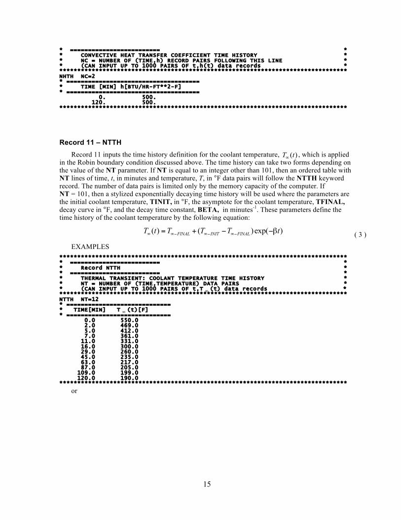
Record 11 – NTTH Record 11 inputs the time history definition for the coolant temperature, ( )T t∞ , which is applied
in the Robin boundary condition discussed above. The time history can take two forms depending on the value of the NT parameter. If NT is equal to an integer other than 101, then an ordered table with NT lines of time, t, in minutes and temperature, T, in °F data pairs will follow the NTTH keyword record. The number of data pairs is limited only by the memory capacity of the computer. If NT = 101, then a stylized exponentially decaying time history will be used where the parameters are the initial coolant temperature, TINIT, in °F, the asymptote for the coolant temperature, TFINAL, decay curve in °F, and the decay time constant, BETA, in minutes-1. These parameters define the time history of the coolant temperature by the following equation:
( ) ( )exp( )FINAL INIT FINALT t T T T t∞ ∞− ∞− ∞−= + − −β ( 3 )
EXAMPLES ******************************************************************************** * ========================= * * Record NTTH * * ========================= * * THERMAL TRANSIENT: COOLANT TEMPERATURE TIME HISTORY * * NT = NUMBER OF (TIME,TEMPERATURE) DATA PAIRS * * (CAN INPUT UP TO 1000 PAIRS OF t,T ∞ (t) data records * ******************************************************************************** NTTH NT=12 * ============================= * TIME[MIN] T ∞ (t)[F] * ============================= 0.0 550.0 2.0 469.0 5.0 412.0 7.0 361.0 11.0 331.0 16.0 300.0 29.0 260.0 45.0 235.0 63.0 217.0 87.0 205.0 109.0 199.0 120.0 190.0 ********************************************************************************
or

16
******************************************************************************** * ========================= * * Record NTTH * * ========================= * * THERMAL TRANSIENT: COOLANT TEMPERATURE TIME HISTORY * * NT = 101 ==> STYLIZED EXPONENTIAL DECAYING COOLANT TEMPERATURE * * * * TINIT = INITIAL COOLANT TEMPERATURE (at time=0) (F) * * TFINAL = LOWEST TEMPERATURE IN TRANSIENT (F) * * BETA = DECAY CONSTANT (MIN**-1) * * * * FAVLoad CALCULATES AND STORES THE COOLANT TEMPERATURE AT * * 100 EQUALLY-SPACED TIME STEPS ACCORDING TO THE RELATION * * * * T ∞ (t) = T ∞ -FINAL + (T ∞ INIT - T ∞ FINAL) * EXP( -BETA*TIME(min) * ******************************************************************************** NTTH NT=101 STYL TINIT=550 TFINAL=190 BETA=0.15 ********************************************************************************
Record 12 – NPTH Record 12 inputs the time history table for the internal coolant pressure boundary condition.
There are NP data pairs of time, t, in minutes and internal coolant pressure, p, in kilo-pounds force per square inch (ksi) entered following the NPTH keyword record line. The number of data pairs is limited only by the memory capacity of the computer.
EXAMPLE ******************************************************************************** * ========================= * * Record NPTH * * ========================= * * PRESSURE TRANSIENT: PRESSURE vs TIME HISTORY * * NP = NUMBER OF (TIME,PRESSURE) DATA PAIRS * * (CAN INPUT UP TO 1000 PAIRS OF t,P(t) data records * ******************************************************************************** NPTH NP=2 * ============================== * TIME[MIN] P(t)[ksi] * ============================== 0.0 1.0 120.0 1.0
Records 13 through 20 are data obtained from Grizzly.
Record 13 – GNTI Record 13 inputs NTIMES_GRI which is the number of time steps available from the Grizzly simulation.
Record 14 – GNME Record 14 inputs NUMNP_GRI which is the number of thru-wall mesh points available from the Grizzly simulation.
Record 15 – Time Discretization from Grizzly Record 15 inputs NTIMES_GRI data lines of (time step[-], time[minutes]) ordered pairs used in the Grizzly simulation.

17
Record 16 – Thru-Wall Mesh Discretization from Grizzly Record 16 inputs NUMNP_GRI data lines of mesh points (as measured from the inner RPV wall) used in the Grizzly simulation.
Record 17 – Internal Pressures from Grizzly Record 17 inputs NTIMES_GRI data lines of internal pressures available from the Grizzly simulation.
Record 18 – Time-dependent Temperature Profiles from Grizzly Record 18 inputs NTIMES_GRI x NUMNP_GRI data lines of time-dependent thru-wall temperature profiles available from the Grizzly simulation.
Record 19 – Time-dependent Hoop Stress Profiles from Grizzly Record 19 inputs NTIMES_GRI x NUMNP_GRI data lines of time-dependent thru-wall hoop stress profiles available from the Grizzly simulation.
Record 20 – Time-dependent Axial Stress Profiles from Grizzly Record 20 inputs NTIMES_GRI x NUMNP_GRI data lines of time-dependent thru-wall axial stress profiles available from the Grizzly simulation.
2.4 Grizzly/FAVOR Interface Output Files
The Grizzly/FAVOR Interface application creates two output ASCII text files:
(1) the load-definition file (a user-defined filename at the time of execution) that will be input to FAVPFM (*.out) and
(2) an *.echo file which provides a date and time stamp of the execution and an echo of the Grizzly/FAVOR Interface input file.
The following gives partial listings of typical Grizzly/FAVOR Interface load-definition and echo files. The name of the Grizzly/FAVOR Interface echo file is constructed from the root of the Grizzly/FAVOR Interface load-definition output file as specified by the user during execution with the “.echo” extension added, e.g., Load1.out ⇒Load1.echo.

18
Grizzly/FAVOR Interface Load-Definition Output File //Version, MTRAN, Emod_Base, nu_Base, Emod_Clad, nu_Clad 121 1 2.800000E+04 3.000000E-01 2.280000E+04 3.000000E-01 //TH Transient Sequence Table 1 7 //RPV Geometry: Rinner, Router, tclad 7.850000E+01 8.653600E+01 1.560000E-01 //Discretization Data Dimensions: NTIMES, NCDH 25 16 //Time Discretization Data: DTIME(1:NTIMES) 1 0.000000E+00 2 1.000000E+01 3 2.000000E+01 4 3.000000E+01 5 4.000000E+01 6 5.000000E+01 7 6.000000E+01 8 7.000000E+01 9 8.000000E+01 10 9.000000E+01 11 1.000000E+02 12 1.100000E+02 13 1.200000E+02 14 1.300000E+02 15 1.400000E+02 16 1.500000E+02 17 1.600000E+02 18 1.700000E+02 19 1.800000E+02 20 1.900000E+02 21 2.000000E+02 22 2.100000E+02 23 2.200000E+02 24 2.300000E+02 25 2.400000E+02 //Mesh Discretization Data: HCD(1:NCDH) 0.000000E+00 8.036000E-02 1.607200E-01 2.410800E-01 4.018000E-01 6.027000E-01 8.036000E-01 1.607200E+00 2.410800E+00 3.214400E+00

19
Grizzly/FAVOR Interface Output Echo File
************************************************ * * * WELCOME TO Grizzly_FAVOR_Interface * * * * VERSION 1.0 * * * * PROBLEMS OR QUESTIONS REGARDING Interface * * SHOULD BE DIRECTED TO * * * * TERRY DICKSON * * OAK RIDGE NATIONAL LABORATORY * * * * e-mail: [email protected] * * * ************************************************ *********************************************************** * This computer program was prepared as an account of * * work sponsored by the United States Government * * Neither the United States, nor the United States * * Department of Energy, nor the United States Nuclear * * Regulatory Commission, nor any of their employees, * * nor any of their contractors, subcontractors, or their * * employees, makes any warranty, expressed or implied, or * * assumes any legal liability or responsibility for the * * accuracy, completeness, or usefulness of any * * information, apparatus, product, or process disclosed, * * or represents that its use would not infringe * * privately-owned rights. * * * *********************************************************** DATE: 22-May-2013 TIME: 07:11:10 INTERFACE INPUT DATASET NAME = FAVLoad1_GRI.in INTERFACE OUTPUT DATASET NAME = GRI.out INTERFACE ECHO INPUT FILE NAME = GRI.echo ************************************************* * ECHO OF INTERFACE INPUT FILE * ************************************************* ******************************************************************************** * ALL RECORDS WITH AN ASTERISK (*) IN COLUMN 1 ARE COMMENT ONLY * ******************************************************************************** * EXAMPLE INPUT DATASET FOR Grizzly_FAVLoad, v1.0 * ******************************************************************************** ==================== * * Record GEOM * * ==================== * *------------------------------------------------------------------------------* * IRAD = INTERNAL RADIUS OF PRESSURE VESSEL [IN] * * W = THICKNESS OF PRESSURE VESSEL WALL (INCLUDING CLADDING) [IN] * * CLTH = CLADDING THICKNESS [IN] * *------------------------------------------------------------------------------* ******************************************************************************** GEOM IRAD=86.0 W=8.75 CLTH=0.25 ******************************************************************************** * =========================== * * Records BASE and CLAD * * =========================== * * THERMO-ELASTIC MATERIAL PROPERTIES FOR BASE AND CLADDING * *------------------------------------------------------------------------------* * K = THERMAL CONDUCTIVITY [BTU/HR-

20
2.5 Grizzly/FAVOR Interface Software Engineering Metrics
The Grizzly/FAVOR Interface is written in Fortran 90/95. To track the source code changes, the Grizzly/FAVOR Interface code is being stored in a Subversion repository. As of Subversion’s revision 8, tag version 1, the Grizzly/FAVOR Interface code has 5666 Lines of Code.

21
3. VERIFICATION
3.1 Initial Benchmarking of FAVOR and Grizzly
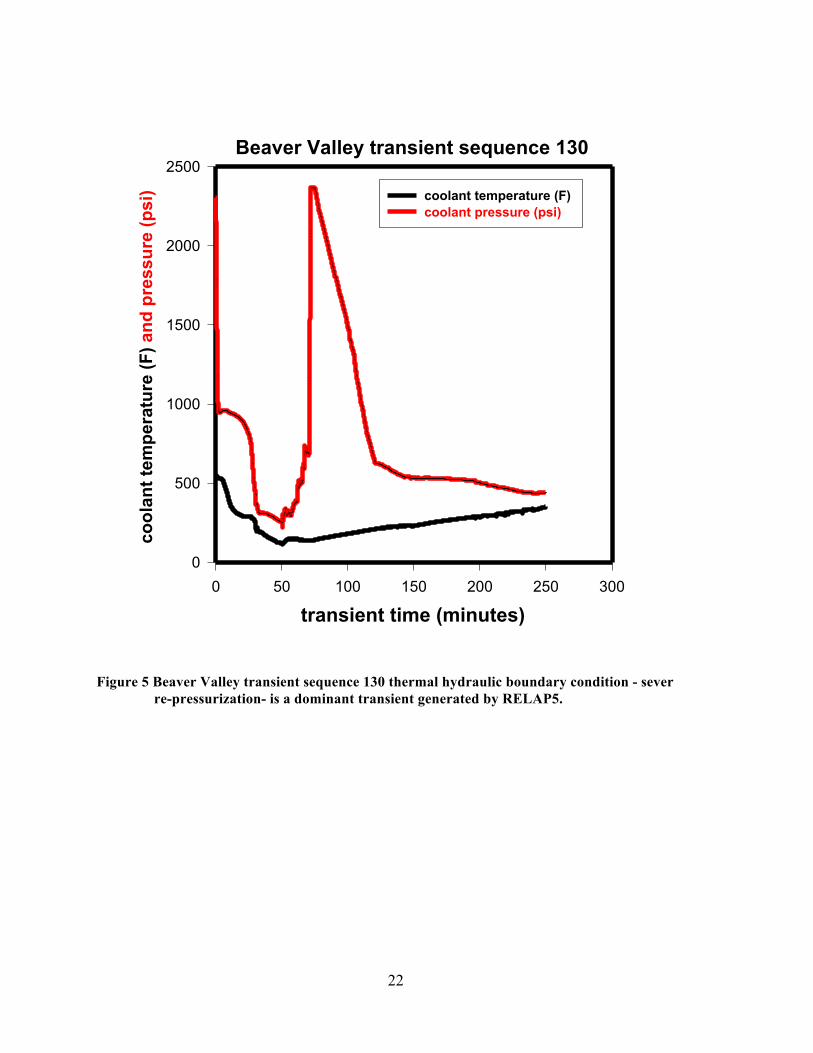
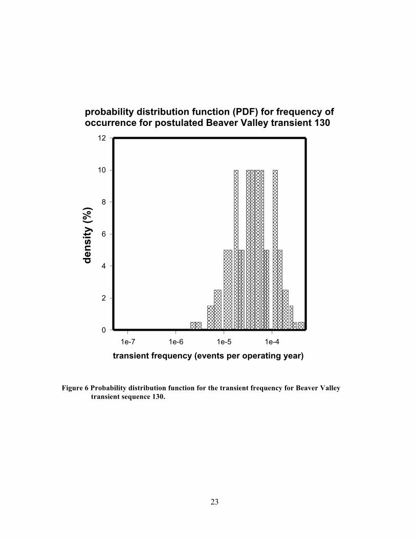
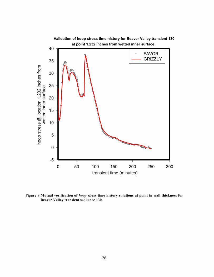
A necessary initial step (in building an interface between Grizzly and FAVOR) is to verify that FAVOR and Grizzly mutually verify each other’s solutions for thermal, hoop stress, and axial stress finite element analyses for complex thermal hydraulic loading imposed on the inner surface of the reactor pressure vessel (RPV). Figure 5 illustrates such a transient. This was transient sequence number 130 postulated for Beaver Valley during the pressurized thermal shock (PTS) re-evaluation. This was one of 61 transients included in the PTS re-evaluation of Beaver Valley. Figure 5 illustrates the coolant temperature and pressure time history boundary conditions that are assumed to be imposed on the inner surface of the RPV. This thermal hydraulic boundary condition was generated by the RELAP5 computer code. Figure 6 illustrates the probability distribution function (PDF) of the frequency of occurrence (events per reactor operating year) of this particular transient actually occurring. This was generated by the SAPHIRE7 computer code. The specific description provided for transient sequence number 130 was as follows: reactor turbine trip with one stuck open pressurizer safety relief which recloses at 3000 seconds. Transient sequence 130 was considered a dominant transient, i.e., it contributed a significant fraction of the total risk for Beaver Valley for all times in the life of the RPV. The primary characteristic of this transient is the re-pressurization that occurs relatively late in the transient after the RPV has cooled down. Transients with this characteristic were found to be the dominant transients for all reactors analyzed in the Pressurized Thermal Shock Re-Evaluation. From Figure 7 through Figure 9 we illustrate that the FAVOR and Grizzly time history solutions for the temperature, axial stress, and hoop stress, respectively, occurring at a specified distance into the RPV wall (measured from the RPV wetted inner surface) are in reasonably good agreement. The verifications provided in Figure 7 - Figure 9 provided assurance that the objectives illustrated in Figure 1 and Figure 4 have been met. It should be noted that the analyses represented in Figure 7 to Figure 9 were performed without the stainless steel clad layer. At the time these initial benchmarking calculations were performed, Grizzly did not have the capability to include the stainless steel clad layer. It is anticipated that additional verification will be performed once Grizzly has been modified to have the capability to include clad layer in the model.
22
Beaver Valley transient sequence 130
transient time (minutes) 0 50 100 150 200 250 300
cool
ant t
empe
ratu
re (F
) and
pre
ssur
e (p
si)
0
500
1000
1500
2000
2500
coolant temperature (F) coolant pressure (psi)
Figure 5 Beaver Valley transient sequence 130 thermal hydraulic boundary condition - sever
re-pressurization- is a dominant transient generated by RELAP5.
23
probability distribution function (PDF) for frequency of occurrence for postulated Beaver Valley transient 130
transient frequency (events per operating year) 1e-7 1e-6 1e-5 1e-4
dens
ity (%
)
0
2
4
6
8
10
12
Figure 6 Probability distribution function for the transient frequency for Beaver Valley
transient sequence 130.

24
Validation of temperature time history for Beaver Valley transient 130 at point 1.232 inches from wetted inner surface
transient time (minutes) 0 50 100 150 200 250 300
tem
pera
ture
(F) a
t loc
atio
n 1.
232
inch
es fr
om w
ette
d in
ner s
urfa
ce
150
200
250
300
350
400
450
500
550
600
FAVOR GRIZZLY
Figure 7 Mutual verification of temperature time history solutions at point in wall thickness for
Beaver Valley transient sequence 130.

25
Validation of axial stress time history for Beaver VAlley transient 130 at point 1.232 inches from wetted inner surface
transient time (minutes) 0 50 100 150 200 250 300
axia
l stre
ss @
loca
tion
1.23
2 in
ches
from
w
ette
d in
nner
sur
face
(ksi
)
-5
0
5
10
15
20
25
30
35FAVOR GRIZZLY
Figure 8 Mutual verification of axial stress time history solutions at point in wall thickness for
Beaver Valley transient sequence 130.
26
Validation of hoop stress time history for Beaver Valley transient 130at point 1.232 inches from wetted inner surface
transient time (minutes) 0 50 100 150 200 250 300
hoop
stre
ss @
loca
tion
1.23
2 in
ches
from
w
ette
d in
ner s
urfa
ce
-5
0
5
10
15
20
25
30
35
40FAVOR GRIZZLY
Figure 9 Mutual verification of hoop stress time history solutions at point in wall thickness for
Beaver Valley transient sequence 130.
27
3.2 Initial Testing of the Grizzly –FAVOR Interface
The objective of the Grizzly-FAVOR interface is to map σhoop(x, t), σaxial(x, t), and Τ(x, t) from any one-dimensional coordinate system to the specific one-dimensional coordinate system (that is output by FAVLOAD) and required as input by FAVPFM as illustrated in Figure 1Figure 1. If this objective is successfully met, the results of Grizzly finite element thermal and stress analyses can be used as input to FAVPFM without requiring any modifications to the FAVPFM. The FAVPFM module is used to perform deterministic and probabilistic fracture mechanics analyses of RPVs subjected to complex thermal hydraulic boundary conditions imposed on their inner surface. Therefore, for purposes of testing the Grizzly-FAVOR interface, σhoop(x, t), σaxial(x, t), and Τ(x, t) data generated in any coordinate system (other than the coordinate system that corresponds to the gauss points used in the finite element analyses) can be used as input into the Grizzly-FAVOR interface. Internally, FAVLOAD and FAVPFM both do mapping of stresses, temperatures, and applied KI as required. For example, σhoop(x, t), σaxial(x, t), and Τ(x, t) are mapped (by piecewise cubic spline) from the gauss points used in the thermal and stress finite element analyses to the following 16 locations that correspond to 0.0, 0.01, 0.02, 0.03, 0.05, 0.075, 0.10, 0.20, 0.30, 0.40, 0.50, 0.60, 0.70, 0.80, 0.90, and 0.95 of the fractional wall thickness. These particular locations correspond to locations for which SIFICs (stress intensity factor influence coefficients) were pre-calculated for infinite length flaws. The SIFICs are used in the calculation of applied stress intensity factors by the method of superposition. In general, during FAVOR deterministic or probabilistic analyses, if values of σhoop(x, t), σaxial(x, t), and Τ(x, t) at a particular location or for values of KI for a particular flaw geometry (other than the 16 depths specified above) are required, then the value(s) are generated (mapped) internally by use of the piecewise cubic spline curve fit. So for purposes of testing the Grizzly-FAVOR interface, σhoop(x, t), σaxial(x, t), and Τ(x, t) data generated by FAVOR in any coordinate system (other than the coordinate system that corresponds to the gauss points used in the finite element analyses) can be used as test input into the Grizzly-FAVOR interface . Figure 10 is an illustration of Beaver Valley transient sequence 007 – a severe cooldown caused by a pipe break. In Figure 11 through Figure 15, the test case is the time history solutions in a coordinate system used for deterministic reporting, whereas, the FAVOR-Grizzly interface solution is the solutions for Τ(x, t), σaxial(x, t), and σhoop(x, t), after the test cases solutions have been mapped to the coordinate system required for input into the FAVPFM module. Similarly, in Figure 16 through Figure 18, the test case is the thru-wall spatial profile solution in a coordinate system used for deterministic reporting, whereas, the FAVOR-Grizzly interface solution is the solution for Τ(x, t), σaxial(x, t), and σhoop(x, t), after the test cases

28
solutions have been mapped to the coordinate system required for input into the FAVPFM module.
Figure 10 Illustration of Beaver Valley transient sequence 007 - a severe cooldown transient
caused by surge line break.

29
Figure 11 Verification of Grizzly-FAVOR interface for temperature - time history at various
locations thru-the-wall thickness

30
Figure 12 Verification of Grizzly-FAVOR interface for axial stress - time history at various
locations thru-the-wall thickness

31
Figure 13 Verification of Grizzly-FAVOR interface for hoop stress-time history at various
locations thru-the-wall thickness.

32
Figure 14 Verification of Grizzly-FAVOR interface for spatial profiles of thru-wall
temperatures at different transient times.

33
Figure 15 Verification of Grizzly-FAVOR interface for spatial profiles of thru-wall axial stress
at different transient times

34
Figure 16 Verification of Grizzly-FAVOR interface for spatial profiles of thru-wall hoop stress
at different transient times.

35
4. Grizzly/FAVOR INTERFACE USER GUIDE
This section describes how to use the Grizzly/FAVOR interface.
4.1 Grizzly/FAVOR Interface Distribution
The Grizzly/FAVOR Interface is distributed in a WINZIP archive file along with the executables of FAVOR V12.1 as shown below.
4.2 Hardware and SOFTWARE Requirements
The FAVOR/Grizzly Interface code has been run and tested in the following environments:
Hardware:
• HP Z400 Workstation (x64-based PC) Intel64 Family 6 Model 26 Stepping 5 GenuineIntel ~2368 Mhz)
• HP Z800 Workstation (X86-based PC) x64 Family 6 Model 26 Stepping 5 GenuineIntel ~1729 Mhz
Operating Systems:

36
• Microsoft Windows 7 Enterprise, version 6.1.7601 Service Pack 1 Build 7601 • Microsoft Windows Vista T Enterprise 6.0.6002 Service Pack 2 Build 6002

37
4.3 Running the Grizzly/FAVOR Interface
This section describes how to run the Grizzly/FAVOR Interface. On Microsoft Windows operating systems (Windows XP/VISTA/7), the following three modules:
1. FAVOR-Grizzly Interface
2. FAVPFM
3. FAVPost
can be started either by double clicking on the executables’ icon (named FAVOR_Grizzly _Interface.exe, FAVPFM.exe, and FAVPost.exe, respectively) in Windows Explorer, or by opening a Command Prompt window and typing in the name of the executable at the line prompt as shown in Figure 17a for FAVOR/Grizzly execution.
All input files and executables must reside in the same current working directory. For details on the creation of FAVOR input files see Chapter 2 of ref. [2]. In Figure 17b, the code prompts for the names of the FAVOR/Grizzly input and FAVOR/Grizzly output files. The FAVOR/Grizzly output file will be used as the load-definition input file for the FAVPFM module. Figure 18 shows the messages written to the screen as FAVOR/Grizzly performs its calculations.
Upon creation of the load-definition file by FAVOR/Grizzly, FAVPFM execution can be started by typing “FAVPFM” at the line prompt (see Figure 19). FAVPFM will then prompt the user for the names of six files (see Figure 20):
(1) the FAVPFM input file,
(2) load-definition file output from FAVOR/Grizzly,
(3) a name for the output file to be created by FAVPFM,
(4) the name of the input flaw-characterization file for surface-breaking flaws in weld and plate regions (DEFAULT=S.DAT),
(5) the name of the flaw-characterization file for embedded flaws in weld regions (DEFAULT=W.DAT), and
(6) the name of the flaw-characterization file for embedded flaws in plate regions (DEFAULT=P.DAT).
The user can accept the default file names for input files (4)-(6) by typing the ENTER key at the prompt. If FAVPFM cannot find the named input files in the current execution directory, it will prompt the user for new file names. If the FAVPFM output file to be created already exists in the current directory, the code will query the user if it should overwrite the file. For RESTART cases, the user will be prompted for the name of a binary restart file created during a previous execution. See Sect. 2.2 of ref. [2], Record 1 – CNT1, for detailed information on the execution of restart cases.
The user may abort the execution at any time by typing a <ctrl>c. FAVPFM provides monitoring information during execution by writing the running averages of conditional probabilities of initiation and vessel failure for all of the transients defined in the load file for each RPV trial as shown in Figure 21.
In Figure 22, FAVOR’s post-processing module is executed by typing FAVPost at the line prompt. The code will then prompt the user for the names of four files (see Figure 22):
(1) a FAVPost input file,
(2) the file created by the FAVPFM execution that contains the conditional probability of initiation matrix (DEFAULT=INITIATE.DAT),

38
(3) the file created by the FAVPFM execution that contains the conditional probability of failure matrix (DEFAULT=FAILURE.DAT), and
(4) the name of the output file to be created by FAVPost that will have the histograms for vessel fracture and failure frequencies.
Again, for files (2) and (3), the user may accept the defaults by typing the RETURN/ENTER key.

39
(a)
(b) Figure 17. Execution of the Grizzly/FAVOR interface module: (a) type in
FAVOR_Grizzly_interface.exe at the line prompt and (b) respond to prompts for the input and output file names

40
Figure 18. The Grizzly/FAVOR interface calculates thermal, stress, and applied KI loading for
all of the transients defined in the input file.

41
Figure 19. Type FAVPFM.EXE at the Command Prompt to begin execution of the FAVPFM
module.

42
Figure 20. FAVPFM prompts for the names of the (1) FAVPFM input file, (2) FAVLoad-
generated load-definition file, (3) FAVPFM output file, (4) flaw-characterization file for surface-breaking flaws in welds and plates, (5) flaw-characterization file for embedded flaws in welds, and (6) flaw-characterization file for embedded flaws in plates.

43
Figure 21. FAVPFM continually writes out progress reports in terms of running average
CPI/CPF values for each transient as the code proceeds through the required number of RPV trials.

44
Figure 22. Type in FAVPost at the Command Prompt to execute the FAVPost module.
FAVPost prompts for the (1) FAVPost input file, (2) CPI matrix file generated by FAVPFM, (3) CPF matrix file generated by FAVPFM, and (4) the FAVPost output file. Set the total number of simulations to be processed and build convergence tables, if required.

45
4.4 Contacts
To obtain a copy of the Grizzly/FAVOR Interface executables, pleaes contact:
• Jeremy Busby: busbyjt at ornl dot gov

46
5. CONCLUSIONS AND FUTURE SUGGESTIONS
This document describes the implementation of the Grizzly/FAVOR Interface project. The objective of the Grizzly/FAVOR Interface is to create the capability to apply Grizzly 3-D finite element (thermal and stress) analysis results as input to FAVOR probabilistic fracture mechanics (PFM) analyses. The one benefit of FAVOR to Grizzly is the PROBABILISTIC capability. This document detailed the implementation of the Grizzly/FAVOR Interface, the preliminary verification and tests results and a user guide that provided detailed step-by-step instructions to run the program.
A work plan for developing a Fracture Mechanics Assessment Capability in Grizzly has been written to detail the future work in [ 5, ORNL-2013-44107].
47
6. REFERENCES
1. P. T. Williams, T. L. Dickson, and S. Yin, Fracture Analysis of Vessels – FAVOR (v12.1)
2. T. L. Dickson, P. T. Williams and S. Yin, Fracture Analysis of Vessels – FAVOR (v12.1) Computer Code: User’s Guide, ORNL/TM-2012/566, Oak Ridge National Laboratory, Oak Ridge, TN, 2012.
3. Light Water Reactor Sustainability Program – Integrated Program Plan, INL/EXT-11-23452, Idaho National Laboratory, Idaho Falls, ID, January 2012.
4. B. Spencer, J. Busby, R. Martineau, B. Wirth, A Proof of Concept: Grizzly, The LWRS Programs Materials Aging and Degradation Pathway Main Simulation Tool.
5. B.R. Bass, T.L. Dickson, H.B. Klasky, and P.T. Williams, Work Plan for Developing a Fracture Mechanics Assessment Capability in GRIZZLY, ORNL-2013-44107, June 2013.