HAL Id: hal-00820599https://hal.inria.fr/hal-00820599

Submitted on 6 May 2013

HAL is a multi-disciplinary open accessarchive for the deposit and dissemination of sci-entific research documents, whether they are pub-lished or not. The documents may come fromteaching and research institutions in France orabroad, or from public or private research centers.

L’archive ouverte pluridisciplinaire HAL, estdestinée au dépôt et à la diffusion de documentsscientifiques de niveau recherche, publiés ou non,émanant des établissements d’enseignement et derecherche français ou étrangers, des laboratoirespublics ou privés.

Gromov-Hausdorff Approximation of Metric Spaces withLinear Structure

Frédéric Chazal, Jian Sun

To cite this version:Frédéric Chazal, Jian Sun. Gromov-Hausdorff Approximation of Metric Spaces with Linear Structure.2013. �hal-00820599�

Gromov-Hausdorff Approximation of Metric Spaces with LinearStructure

Frederic Chazal ∗, Jian Sun †

May 6, 2013

Abstract

In many real-world applications data come as discrete metric spaces sampled around 1-dimensionalfilamentary structures that can be seen as metric graphs. In this paper we address the metric recon-struction problem of such filamentary structures from data sampled around them. We prove that theycan be approximated, with respect to the Gromov-Hausdorff distance by well-chosen Reeb graphs(and some of their variants) and we provide an efficient and easy to implement algorithm to computesuch approximations in almost linear time. We illustrate the performances of our algorithm on a fewsynthetic and real data sets.

1 Introduction

Motivation. With the advance of sensor technology, computing power and Internet, massive amountsof geometric data are being generated and collected in various areas of science, engineering and business.As they are becoming widely available, there is a real need to analyze and visualize these large scalegeometric data to extract useful information out of them. In many cases these data are not embedded inEuclidean spaces and come as (finite) sets of points with pairwise distances information, i.e. (discrete)metric spaces. A large amount of research has been done on dimensionality reduction, manifold learningand geometric inference for data embedded in, possibly high dimensional, Euclidean spaces and assumedto be concentrated around low dimensional manifolds [5, 29, 34]. However, the assumption of data lyingon a manifold may fail in many applications. In addition, the strategy of representing data by pointsin Euclidean space may introduce large metric distortions as the data may lie in highly curved spaces,instead of in flat Euclidean space raising many difficulties in the analysis of metric data. In the pastdecade, with the development of topological methods in data analysis, new theories such as topologicalpersistence (see, for example, [21, 36, 8, 10]) and new tools such as the Mapper algorithm [33] havegiven rise to new algorithms to extract and visualize geometric and topological information from metricdata without the need of an embedding into an Euclidean space. In this paper we focus on a simplebut important setting where the underlying geometric structure approximating the data can be seen asa branching filamentary structure i.e., more precisely, as a metric graph which is a topological graphendowed with a length assigned to each edge (see Section 2). Such structures appear naturally in variousreal-world data such as collections of GPS traces collected by vehicles on a road network, earthquakesdistributions that concentrate around geological faults, distributions of galaxies in the universe, networksof blood vessels in anatomy or hydrographic networks in geography just to name a few of them. It is thusappealing to try to capture such filamentary structures and to approximate the data by metric graphs thatwill summarize the metric and allow convenient visualization.∗INRIA Saclay - France - frederic.chazal@inria.fr†Tsinghua University - China

1

Contribution In this paper we address the metric reconstruction problem for filamentary structures.The input of our method and algorithm is a metric space (X, dX) that is assumed to be close withrespect to the so-called Gromov-Hausdorff distance dGH to a much simpler, but unknown, metric graph(G′, dG′). Our algorithm outputs a metric graph (G, dG) that is proven to be close to (X, dX). Ourapproach relies on the notion of Reeb graph (and some variants of it introduced in Section 3.1) and oneof our main theoretical result can be stated as follows.

Theorem 3.10. Let (X, dX) be a compact connected geodesic space, let r ∈ X be a fixed base pointsuch that the metric Reeb graph (G, dG) of the function d = dX(r, .) : X → R is a finite graph. If for agiven ε > 0 there exists a finite metric graph (G′, dG′) such that dGH(X,G′) < ε then we have

dGH(X,G) < 2(β1(G) + 1)(17 + 8NE,G′(8ε))ε

where NE,G′(8ε) is the number of edges of G′ of length at most 8ε and β1(G) is the first Betti numberof G, i.e. the number of edges to remove from G to get a spanning tree. In particular if X is at distanceless than ε from a metric graph with shortest edge larger than 8ε then dGH(X,G) < 34(β1(G) + 1)ε.

Turning this result into a practical algorithm requires to address two issues:

- First, raw data usually do not come as geodesic spaces. They are given as discrete sets of point(and thus not connected metric spaces) sampled from the underlying space (X, dX). Moreover inmany cases only distances between nearby points are known. A geodesic space (see Section 2 fora definition of geodesic space) can then be obtained from these raw data as a neighborhood graphwhere nearby points are connected by edges whose length is equal to their pairwise distance. Theshortest path distance in this graph is then used as the metric. In our experiments we use this newmetric as the input of our algorithm. The question of the approximation of the metric on X by themetric induced on the neighborhood graphs is out of the scope of this paper.

- Second, approximating the Reeb graph (G, dG) from a neighborhood graph is usually not obvious.If we compute the Reeb graph of the distance function to a given point defined on the neighbor-hood graph we obtain the neighborhood graph itself and do not achieve our goal of representingthe input data by a simple graph. It is then appealing to build a two dimensional complex havingthe neighborhood graph as 1-dimensional skeleton and use the algorithm of [27, 31] to computethe Reeb graph of the distance to the root point. Unfortunately adding triangles to the neighbor-hood graph may widely change the metric between the data points on the resulting complex andsignificantly increase the complexity of the algorithm. We overcome this issue by introducing avariant of the Reeb graph, the α-Reeb graph, inspired from [33] and related to the recently intro-duced notion of graph induced complex [14], that is easier to compute than the Reeb graph butalso comes with approximation guarantees (see Theorem 3.11). As a consequence our algorithmrelies on the Mapper algorithm of [33] and runs in almost linear time (see Section 4).

Related work. Approximation of data by 1-dimensional geometric structures has been considered bydifferent communities. In statistics, several approaches have been proposed to address the problem ofdetection and extraction of filamentary structures in point cloud data. For example Arial-Castro et al[4] use multiscale anisotropic strips to detect linear structure while [24, 23] and more recently [25] basetheir approach upon density gradient descents or medial axis techniques. These methods apply to datacorrupted by outliers embedded in Euclidean spaces and focus on the inference of individual filamentswithout focus on the global geometric structure of the filaments network.

In computational geometry, the curve reconstruction problem from points sampled on a curve inan euclidean space has been extensively studied and several efficient algorithms have been proposed[3, 16, 17]. Unfortunately, these methods restricts to the case of simple embedded curves (withoutsingularities or self-intersections) and hardly extend to the case of topological graphs. In a more intrinsicsetting where data come as finite abstract metric spaces, [1] propose an algorithm that outputs, undersome specific sampling conditions, a topologically correct (up to a homeomorphism) reconstruction of

2

the approximated graph. However this algorithm requires some tedious parameters tuning and relieson quite restrictive sampling assumptions. When these conditions are not satisfied, the algorithm mayfail and not even outputs a graph. Compared to the algorithm of [1], our algorithm not only comeswith metric guarantees but also whatever the input data is, it always outputs a metric graph and does notrequire the user to choose any parameters. Our approach is also related to the so-called Mapper algorithm[33] that provides a way to visualize data sets endowed with a real valued function as a graph. Indeedthe implementation of our algorithm relies on the Mapper algorithm where the considered function is thedistance to the chosen root point. However, unlike the general mapper algorithm, our methods providesan upper bound on the Gromov-Hausdorff distance between the reconstructed graph and the underlyingspace from which the data points have been sampled.

In theoretical computer science, there is much of work on approximating metric spaces using trees[7, 2, 12] or distribution of trees [18, 22] where the trees are often constructed as spanning trees possiblywith Steiner points. Our approach is different as our reconstructed graph or tree is a quotient space ofthe original metric space where the metric only gets contracted (see Lemma 3.6). Finally we remarkthat the recovery of filament structure is also studied in various applied settings, including road networks[11, 35], galaxies distributions [13].

The paper is organized as follows. The basic notions and definitions used throughout the paper arerecalled in Section 2. The Reeb and α-Reeb graphs endowed with a natural metric are introduced inSection 3.1 and the approximation results are stated and proven in Sections 3.2 and 3.3. Our algorithmis described in Section 4 and experimental results are presented and discussed in Section 5.

2 Preliminaries: metric spaces, metric graphs and Gromov-Hausdorffdistance

Recall that a metric space is a pair (X, dX) where X is a set and dX : X × X → R is a non negativemap such that for any x, y, z ∈ X , dX(x, y) = 0 if and only if x = y, dX(x, y) = dX(y, x) anddX(x, z) 6 dX(x, y) + dX(y, z). Two compact spaces (X, dX) and (Y, dY ) are isometric if there exitsa bijection ϕ : X → Y that preserves the distances, namely: for any x, x′ ∈ X, dY (ϕ(x), ϕ(x′)) =dX(x, x′). The set of isometry classes of compact metric spaces can be endowed with a metric, the so-called Gromov-Hausdorff distance that can be defined using the following notion of correspondence ([6]Def. 7.3.17).

Definition 2.1. Let (X, dX) and (Y, dY ) be two compact metric spaces. Given ε > 0, an ε-correspondencebetween (X, dX) and (Y, dY ) is a subset C ⊂ X × Y such that:i) for any x ∈ X there exists y ∈ Y such that (x, y) ∈ C;ii) for any y ∈ Y there exists x ∈ X such that (x, y) ∈ C;iii) for any (x, y), (x′, y′) ∈ C, |dX(x, x′)− dY (y, y′)| 6 ε.

Definition 2.2. The Gromov-Hausdorff distance between two compact metric spaces (X, dX) and (Y, dY )is defined by

dGH(X,Y ) =1

2inf{ε > 0 : there exists an ε-correspondence between X and Y }

A metric space (X, dX) is a path metric space if the distance between any pair of points is equalto the infimum of the lengths of the continuous curves joining them 1. Equivalently (X, dX) is apath metric space if and only if for any x, y ∈ X and any ε > 0 there exists z ∈ X such thatmax(dX(x, z), dX(y, z)) 6 1

2dX(x, y) + ε [26]. In the sequel of the paper we consider compact pathmetric spaces. It follows from the Hopf-Rinow theorem (see [26] p.9) that such spaces are geodesic, i.e.

1see [26] Chap.1 for the definition of the length of a continuous curve in a general metric space

3

for any pair of point x, x′ ∈ X there exists a minimizing geodesic joining them.2 A continuous pathδ : I → X where I is a real interval or the unit circle is said to be simple if it is not self intersecting, i.e.if δ is an injective map.

Recall that a (finite) topological graph G = (V,E) is the geometric realisation of a (finite) 1-dimensional simplicial complex with vertex set V and edge set E. If moreover each 1-simplex e ∈ Eis a metric edge, i.e. e = [a, b] ⊂ R, then the graph G inherits from a metric dG which is the uniqueone whose restriction to any e = [a, b] ∈ E coincides with the standard metric on the real segment [a, b].Then (G, dG) is a metric graph (see [6], Section 3.2.2 for a more formal definition). Intuitively, a metricgraph can be seen as a topological graph with a length assigned to each of its edges.

The first Betti number β1(G) of a finite topological graph G is the rank of the first homology groupof G (with coefficient in a field, e.g. Z/2), or equivalently, the number of edges to remove from G to geta spanning tree.

3 Approximation of path metric spaces with Reeb-like graphs

Let (X, dX) be a compact geodesic space and let r ∈ X be a fixed base point. Let d : X → R be thedistance function to r, i.e., d(x) = dX(r, x).

3.1 The Reeb and α-Reeb graphs of d

The Reeb graph. The relation x ∼ y if and only if d(x) = d(y) and x, y are in the same path connectedcomponent of d−1(d(x)) is an equivalence relation. The quotient space G = X/ ∼ is called the Reebgraph of d and we denote by π : X → G the quotient map. Notice that π is continuous and as X ispath connected, G is path connected. The function d induces a function d∗ : G → R+ that satisfiesd = d∗ ◦ π. The relation defined by: for any g, g′ ∈ G, g 6G g′ if and only if d∗(g) 6 d∗(g

′) and thereexist a continuous path γ in G connecting g to g′ such that d ◦ γ is non decreasing, makes G a partiallyordered set.

The α-Reeb graphs. Computing or approximating the Reeb graph of (X, d) from a finite set of pointsampled on X is usually a difficult task. To overcome this issue we also consider a variant of the Reebgraph that shares very similar properties than the Reeb graph. Let α > 0 and let I = {Ii}i ∈ I be acovering of the range of d by open intervals of length at most α. The transitive closure of the relationx ∼α y if and only if d(x) = d(y) and x, y are in the same path connected component of d−1(Ii)for some interval Ii ∈ I is an equivalence relation that is also denoted by ∼α. The quotient spaceGα = X/ ∼α is called the α-Reeb graph3 of d and we denote by π : X → Gα the quotient map. Noticethat π is continuous and asX is path connected, Gα is path connected. The function d induces a functiond∗ : Gα → R+ that satisfies d = d∗ ◦ π. The relation defined by: for any g, g′ ∈ Gα, g 6Gα g

′ if andonly if d∗(g) 6 d∗(g

′) and there exist a continuous path γ in Gα connecting g to g′ such that d ◦ γ is nondecreasing, makes Gα a partially ordered set.

The α-Reeb graph is closely related to the graph constructed by the Mapper algorithm introduced in[33] making its computation much more easier than the Reeb graph (see Section 4).

Notice that without making assumptions onX and d, in generalG andGα are not finite graphs. Howeverwhen the number of path connected components of the level sets of d is finite and changes only a finitenumber of times then the Reeb graph turns out to be a finite directed acyclic graph. Similarly, when thecovering of X by the connected components of d−1(Ii), i ∈ I is finite, the α-Reeb graph also turns outto be a finite directed acyclic graph. This happens in most applications and for example when (X, dX) is

2recall that a minimizing geodesic in X is any curve γ : I → X , where I is a real interval, such that dX(γ(t), γ(t′)) =|t− t′| for any t, t′ ∈ I .

3strictly speaking we should call it the α-Reeb graph associated to the covering I but we assume in the sequel that somecovering I has been chosen and we omit it in notations

4

a finite simplicial complex or a compact semialgebraic (or more generally a compact subanalytic space)with d being semi-algebraic (or subanalytic).

All the results and proofs presented in Section 3 are exactly the same for the Reeb and the α-Reeb graphs.In the following paragraph and in Section 3.2,G denotes indifferently the Reeb graph or an α-Reeb graphfor some α > 0. We also always assume that X and d (and α and I) are such that G is a finite graph.

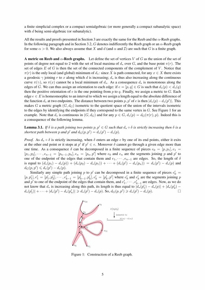
A metric on Reeb and α-Reeb graphs. Let define the set of vertices V of G as the union of the set ofpoints of degree not equal to 2 with the set of local maxima of d∗ over G, and the base point π(r). Theset of edges E of G is then the set of the connected components of the complement of V . Notice thatπ(r) is the only local (and global) minimum of d∗: since X is path connected, for any x ∈ X there existsa geodesic γ joining r to x along which d is increasing; d∗ is thus also increasing along the continuouscurve π(γ), so π(x) cannot be a local minimum of d∗. As a consequence d∗ is monotonous along theedges of G. We can thus assign an orientation to each edge: if e = [p, q] ∈ G is such that d∗(p) < d∗(q)then the positive orientation of e is the one pointing from p to q. Finally, we assign a metric to G. Eachedge e ∈ E is homeomorphic to an interval to which we assign a length equal to the absolute difference ofthe function d∗ at two endpoints. The distance between two points p, p′ of e is then |d∗(p)−d∗(p′)|. Thismakes G a metric graph (G, dG) isometric to the quotient space of the union of the intervals isometricto the edges by identifying the endpoints if they correspond to the same vertex in G. See Figure 1 for anexample. Note that d∗ is continuous in (G, dG) and for any p ∈ G, d∗(p) = dG(π(r), p). Indeed this isa consequence of the following lemma.

Lemma 3.1. If δ is a path joining two points p, p′ ∈ G such that d∗ ◦ δ is strictly increasing then δ is ashortest path between p and p′ and dG(p, p′) = d∗(p

′)− d∗(p).

Proof. As d∗ ◦ δ is strictly increasing, when δ enters an edge e by one of its end points, either it exitsat the other end point or it stops at p′ if p′ ∈ e. Moreover δ cannot go through a given edge more thanone time. As a consequence δ can be decomposed in a finite sequence of pieces e0 = [p, p1], e1 =[p1, p2], · · · , en−1 = [pn−1, pn], en = [pn, p

′] where e0 and en are the segments joining p and p′ toone of the endpoint of the edges that contain them and e1, · · · , en−1 are edges. So, the length of δis equal to (d∗(p1) − d∗(p)) + (d∗(p2) − d∗(p1)) + · · · + (d∗(p

′) − d∗(pn)) = d∗(p′) − d∗(p) and

dG(p, p′) 6 d∗(p′)− d∗(p).

Similarly any simple path joining p to p′ can be decomposed in a finite sequence of pieces e′0 =[p, p′1], e

′1 = [p′1, p

′2], · · · , e′k−1 = [p′k−1, p

′k], e

′k = [p′k, p

′] where e′0 and e′k are the segments joining pand p′ to one of the endpoint of the edges that contain them, and e′1, · · · , e′k−1 are edges. Now, as we donot know that d∗ is increasing along this path, its length is thus equal to |d∗(p′1) − d∗(p)| + |d∗(p′2) −d∗(p

′1)|+ · · ·+ |d∗(p′)− d∗(p′n)| > d∗(p

′)− d∗(p). So, dG(p, p′) > d∗(p′)− d∗(p).

v7

v8

v10v9

v11

v6 v5

r v1v4

v3

v2

e(v8v9)

isometric to

0 |d∗(v9)− d∗(v8)|

Figure 1: Construction of a Reeb graph.

5

3.2 Bounding the Gromov-Hausdorff distance between X and G

The goal of this section is to provide an upper bound of the Gromov-Hausdorff distance between X andG that only depends on the first Betti number β1(G) of G and the maximal diameter M of the level setsof π. An upper bound of M is given in the next section.

Theorem 3.2. dGH(X,G) < (β1(G) + 1)M where dGH(X,G) is the Gromov-Hausdorff distancebetween X and G, β1(G) is the first Betti number of G and M = supp∈G{diameter(π−1(p))} is thesupremum of the diameters of the level sets of π.

The proof of Theorem 3.2 will be easily deduced from a sequence of technical lemmas that al-low to compare the distance between pair of points x, y ∈ X and the distance between their imagesπ(x), π(y) ∈ G.

A vertex v ∈ V is called a merging vertex if it is the end point of at least two edges e1 and e2 that arepointing to it according to the orientation defined in Section 3.1. Geometrically this means that there areat least two distinct connected components of π−1(d−1∗ (d∗(v)− ε)) that accumulate to π−1(v) as ε > 0goes to 0. The set of merging vertices is denoted by Vm.

The following lemma provides an upper bound on the number of vertices in Vm.

Lemma 3.3. The number of elements in Vm is equal to β1(G) where β1(G) is the first homology groupof G.

Proof. The result follows from classical homology persistence theory [20]. First remark that, as π(r) isthe only local minimum of d∗, the sublevel sets of the function d∗ : G → R+ are all path connected.Indeed if π(x), π(y) ∈ G are in the same sublevel set d−1∗ ([0, α]), α > 0, then the images by π ofthe shortest paths in X connecting x to r and y to r are contained in d−1∗ ([0, α]) and their union is acontinuous path joining π(x) to π(y). As a consequence, the 0-dimensional persistence of d∗ is trivial.So, for the persistence algorithm applied to d∗, the vertices of Vm are the positive simplices (see [21] forthe notion of positive and negative simplices for persistence). It follows that each vertex of Vm createsa cycle that never dies as G is one dimensional and does not contain any 2-dimensional simplex. Thus|Vm| = β1(G).

Lemma 3.4. Let p, p′ ∈ G and let δ : [d∗(p), d∗(p′)]→ G be a strictly increasing path going from p to p′

that does not contain any point of Vm in its interior. Then for any x′ ∈ π−1(p′)∩cl(π−1(δ(d∗(p), d∗(p′)))where cl(.) denotes the closure, there exists a shortest path γ connecting a point x of π−1(p) to x′ suchthat π(γ) = δ and dX(x, x′) = d(x′)− d(x) = d∗(p

′)− d∗(p) = dG(p, p′).

Notice that from Lemma 3.1, δ is a shortest path and the parametrization by the interval [d∗(p), d∗(p′)]

can be chosen to be an isometric embedding.

Proof. First assume that p′ is not a merging point. Let γ0 : [0, d(x′)]→ X be any shortest path betweenr and x′ and let γ be the restriction of γ0 to [d∗(p), d(x′)] = [d∗(p), d∗(p

′)]. If the infimum t0 of the setI = {t ∈ [d∗(p), d∗(p

′)] : π(γ(t′)) ∈ δ, ∀t′ > t} is larger than d∗(p), then π(γ(t0)) then there exists anincreasing sequence (tn) that converges to t0 such that γ(tn) 6∈ δ. As a consequence δ(t0) is a mergingpoint; a contradiction. So t0 = d∗(p) and γ(d∗(p)) intersects π−1(p) at a point x.

Now if p′ is a merging point, as x′ is chosen in the closure of π−1(δ(d∗(p), d∗(p′)), for any sufficientlylarge n ∈ N one can consider a sequence of points x′n ∈ π−1(δ(d∗(p′)− 1/n)) that converges to x′ andapply the first case to get a sequence of shortest path γn from a point xn ∈ π−1(p) and x′n. Thenapplying Arzela-Ascoli’s theorem (see [19] 7.5) we can extract from γn a sequence of points convergingto a shortest path γ between a point x ∈ π−1(p) and x′.

To conclude the proof, notice that from Lemma 3.1 we have dG(p, p′) = d∗(p′) − d∗(p) = d(x′) −

d(x). Since γ is the restriction of a shortest path from r to x we also have dX(x, x′) = d(x′)−d(x).

Lemma 3.5 and Lemma 3.6 allow to compare the metrics dX and dG.

6

Lemma 3.5. For any x, y ∈ X we have

dX(x, y) 6 dG(π(x), π(y)) + 2(β1(G) + 1)M

where β1(G) is the first Betti number of G and M = supp∈G{diameter(π−1(p))}.Proof. Let δ be a shortest path between π(x) and π(y). Remark that except at the points π(x) and π(y)the local maxima of the restriction of d∗ to δ are in Vm. Indeed as δ is a shortest path it has to be simple,so if p ∈ δ is a local maximum then p has to be a vertex and δ has to pass through two edges having p asend point and pointing to p according to the orientation defined in Section 3.1. So p is a merging point.Since δ is simple and Vm is finite, δ can be decomposed in at most |Vm| + 1 connected paths along theinterior of which the restriction of d∗ does not have any local maxima. So along each of these connectedpaths the restriction of d∗ can have at most one local minimum. As a consequence, δ can be decomposedin a finite number of continuous paths δ1, δ2, · · · , δk with k 6 2(|Vm| + 1), such that the restriction ofd∗ to each of these path is strictly monotonous. For any i ∈ {1, · · · , k} let pi and pi+1 the end pointsof δi with p1 = π(x) and pk+1 = π(y). We can apply Lemma 3.4 to each δi to get a shortest pathγi in X between a point xi ∈ π−1(pi) and a point in yi+1 ∈ π−1(pi+1) such that π(γi) = δi anddX(xi, yi+1) = dG(pi, pi+1). The sum of the lengths of the paths γi is equal to the sum of the lengthsof the path δi which is itself equal to dG(π(x), π(y)). Now for any i ∈ {1, · · · , k}, since π(xi) = π(yi)we have dX(xi, yi) 6M and xi and yi can be connected by a path of length at most M (x1 is connectedto x and yk+1 is connected to y. Gluing these paths to the paths γi gives a continuous path from x to ywhose length is at most dG(π(x), π(y)) + kM 6 dG(π(x), π(y)) + 2(|Vm|+ 1)M . Since from Lemma3.3, |Vm| 6 β1(G), we finally get that dX(x, y) 6 dG(π(x), π(y)) + 2(β(G) + 1)M .

Lemma 3.6. The map π : X → G is 1-Lipschitz: for any x, y ∈ X we have

dG(π(x), π(y)) 6 dX(x, y).

Proof. Let x, y ∈ X and let γ : I → X be a shortest path from x to y in X where I ⊂ R is a closedinterval. The path π(γ) connects π(x) and π(y) in G.

We first claim that there exists a continuous path Γ contained in π(γ) connecting π(x) and π(y) thatintersects each vertex ofG at most one time. The path Γ can be defined by iteration in the following way.Let v1, · · · vn ∈ V be the vertices of G that are contained in π(γ) \ {π(x), π(y)} and let Γ0 = π(γ) :J0 = I → G. For i = 1, · · ·n let t−i = inf{t : Γi−1(t) = vi} and t+i = sup{t : Γi−1(t) = vi} anddefine Γi as the restriction of Γi−1 to Ji = Ji−1 \ (t−i , t

+i ). The path Γi is a connected continuous path

(although Ji is a disjoint union of intervals) that intersects the vertices v1, v2, · · · , vi at most one time.We then define Γ = Γn : J = Jn → G where J ⊂ I is a finite union of closed intervals. Notice that Γis the image by π of the restriction of γ to J and that Γ(t) ∈ {v1, · · · vn} only if t is one of the endpointsof the closed intervals defining J .

Now, for each connected component [t, t′] of J , γ((t, t′)) is contained in π−1(e) where e is the edgeof G containing Γ([t, t′]). As a consequence, dG(π(γ)(t), π(γ)(t′)) = |d∗(π(γ)(t) − d∗(π(γ)(t′))| =|d(γ(t)) − d(γ(t′))|. Recalling that d(γ(t)) = dX(r, γ(t)) and d(γ(t′)) = dX(r, γ(t′)) and using thetriangle inequality we get that |d(γ(t))− d(γ(t′))| 6 dX(γ(t), γ(t′)). To conclude the proof, since γ isa geodesic path we just need to sum up the previous inequality over all connected components of J :

dX(x, y) >∑

[t,t′]∈cc(J)

dX(γ(t), γ(t′)) >∑

[t,t′]∈cc(J)

dG(π(γ)(t), π(γ)(t′)) > dG(π(x), π(y))

where cc(J) is the set of connected components of J .

The proof of Theorem 3.2 now easily follows from Lemmas 3.5 and 3.6.

Proof. (of Theorem 3.2) Consider the set C = {(x, π(x)) : x ∈ X} ⊂ X × G. As π is surjec-tive this is a correspondence between X and G. It follows from Lemmas 3.5 and 3.6 that for any(x, π(x)), (y, π(y)) ∈ C,

|dX(x, y)− dG(π(x), π(y))| 6 2(β1(G) + 1)M

7

where β1(G) is the first Betti number of G and M = supp∈G{diameter(π−1(p))}. So C is a (2(β1(G)+1)M -correspondence and dGH(X,G) 6 (β1(G) + 1)M .

3.3 Bounding M

To upperbound the diameter of the level sets of π we first prove the two following general lemmas.

Lemma 3.7. Let (G, dG) be a connected finite metric graph and let r ∈ G. We denote by dr = dG(r, .) :G → [0,+∞) the distance to r. For any edge E ⊂ G, the restriction of dr to e is either strictlymonotonous or has only one local maximum. Moreover the length l = l(E) of E is upper bounded bytwo times the difference between the maximum and the minimum of dr restricted to E.

Proof. Let l be the length of E and let t 7→ e(t), t ∈ [0, l], be an arc length parametrization of E. SinceE is an edge of G, for t ∈ [0, l] any shortest geodesic γt joining r to e(t) must contain either x1 = e(0)or x2 = e(l). If it contains x1 then for any t′ < t the restriction of γt between r and e(t′) is a shortestgeodesic containing x1 and if it contains x2 then for any t′ > t the restriction of γt between r and e(t′) isa shortest geodesic containing x2. Moreover in both cases, the function dr is strictly monotonous alongγ. As a consequence, the set I1 = {t ∈ [0, l] : a shortest geodesic joining r to e(t) contains x1} is aclosed interval containing 0. Similarly the set I2 = {t ∈ [0, l] : a shortest geodesic joining r to e(t)contains x2} is a closed interval containing l and [0, l] = I1 ∪ I2. Moreover dr is strictly monotonouson e(I1) and on e(I2). As a consequence I1 ∩ I2 is reduced to a single point t0 that has to be the uniquelocal maximum of dr restricted to E.

The second part of the lemma follows easily from the previous proof: the minimum of dr restrictedto E is attained either at x1 or x2 and dr(e(t0)) = dr(x1) + t0 = dr(x2) + l − t0 is the maximum of drrestricted to E. We thus obtain that 2t0 = l + (dr(x2)− dr(x1)). As a consequence if dr(x1) 6 dr(x2)then l/2 6 t0 = dr(e(t0)) − dr(x1); similarly if dr(x1) > dr(x2) then l/2 6 l − t0 = dr(e(t0)) −dr(x2).

Lemma 3.8. Let (G, dG) be a connected finite metric graph and let r ∈ G. For α > 0 we denote byNE(α) the number of edges of G of length at most α. For any d > 0 and any connected component B ofthe set Bd,α = {x ∈ G : d− α 6 dG(r, x) 6 d+ α} we have

diam(B) 6 4(2 +NE(4α))α

The example of figure 2 shows that the bound of Lemma 3.8 is tight.

r

d− α

4α

B

Figure 2: Tightness of the bound in Lemma 3.8: there are 3 edges of length at most 4α and the diameterof B is equal to 20α.

Proof. Let x, y ∈ B and let t 7→ γ(t) ∈ B be a continuous path joining x to y in B. Let E be an edge ofG that does not contain x or y and with end points x1, x2 such that γ intersects the interior of E. Thenγ−1(E) is a disjoint union of closed intervals of the form I = [t, t′] where γ(t) and γ(t′) belong to the

8

set {x1, x2}. If γ(t) = γ(t′) we can remove the part of γ between t and t′ and still get a continuouspath between x and y. So without loss of generality we can assume that if γ intersects the interior ofE, then E is contained in γ. Using the same argument as previously we can also assume that if γ goesacross E, it only does it one time, i.e. γ−1(E) is reduced to only one interval. As a consequence, γ canbe decomposed in a sequence [x, v0], E1, E2, ·, Ek, [vk, y] where [x, v0] and [vk, y] are pieces of edgescontaining x and y respectively and E1 = [v0, v1], E2 = [v1, v2]·, Ek = [vk−1, vk] are pairwise distinctedges of G contained in B. It follows from Lemma 3.7 that the lengths of the edges E1, · · ·Ek andof [x, v0] and [vk, y] are upper bounded by 4α. As a consequence the length of γ is upper bounded by4(k + 2)α which is itself upper bounded by 4(NE(4α) + 2)α since the edges E1, · · ·Ek are pairwisedistinct. It follows that dG(x, y) 6 4(NE(4α) + 2)α.

Theorem 3.9. Let (G, dG) be a connected finite metric graph and let (X, dX) be a compact geodesicmetric space such that dGH(X,G) < ε for some ε > 0. Let x0 ∈ X be a fixed point and let dx0 =dX(x0, .) : X → [0,+∞) be the distance function to x0. Then for d > α > 0 the diameter of anyconnected component L of d−1x0 ([d− α, d+ α]) satisfies

diam(L) 6 4(2 +NE(4(α+ 2ε)))(α+ 2ε) + ε

where NE(4(α + 2ε)) is the number of edges of G of length at most 4(α + 2ε). In particular if α = 0and 8ε is smaller that the length of the shortest edge of G then the diameter of L is upper bounded by17ε.

Proof. Let ε′ > 0 be such that dGH(X,G) < ε′ < ε. Let C ⊂ X ×G be an ε′-correspondence betweenX and G and (x0, r) ∈ C. we denote by dr = dG(r, .) : G → [0,+∞) the distance function to r in G.Let xa, xb ∈ L and let (xa, ya), (xb, yb) ∈ C. There exists a continuous path γ ⊆ L joining xa to xb.Since C is an ε′-correspondence for any x ∈ γ there exists a point (x, y) ∈ C such that d − α − ε′ 6dr(y) 6 d+α+ε′. The set of points y obtained in this way is not necessarily a continuous path from ya toyb. However one can consider a finite sequence x1 = xa, x2, · · · , xn = xb of points in γ such that for anyi = 1, · · ·n−1 we have dX(xi, xi+1) < ε−ε′. If (xi, yi) ∈ C then we have dG(yi, yi+1) < ε−ε′+ε′ = ε.As a consequence, since d − α − ε < d − α − ε′ < dr(yi) < d + α + ε′ < d + α + ε the shortestgeodesic connecting yi to yi+1 inG remains in the set d−1r ([d−α−2ε, d+α+2ε]) and connecting thesegeodesics for all i = 1, · · · , n−1 we get a continuous path from ya to yb in d−1r ([d−α−2ε, d+α+2ε]).It then follows from Proposition 3.8 that dG(ya, yb) 66 4(2 +NE(4(α+ 2ε)))(α+ 2ε) and since C isan ε′-correspondence (and so an ε-correspondence), dX(xa, xb) < 4(2 +NE(4(α+ 2ε)))(α+ 2ε) + ε.

As a corollary of the Theorem 3.9 and Theorem 3.2 we immediately obtain the following results forthe Reeb graph and the α-Reeb graphs.

Theorem 3.10. Let (X, dX) be a compact connected path metric space, let r ∈ X be a fixed base pointsuch that the metric Reeb graph (G, dG) of the function d = dX(r, .) : X → R is a finite graph. If for agiven ε > 0 there exists a finite metric graph (G′, dG′) such that dGH(X,G′) < ε then we have

dGH(X,G) < (β1(G) + 1)(17 + 8NE,G′(8ε))ε

where NE,G′(8ε) is the number of edges of G′ of length at most 8ε. In particular if X is at distance lessthan ε from a metric graph with shortest edge length larger than 8ε then dGH(X,G) < 17(β1(G) + 1)ε.

Theorem 3.11. Let (X, dX) be a compact connected path metric space. Let r ∈ X , α > 0 and I be afinite covering of the segment [0,Diam(X)] by open intervals of length at most α such that the α-Reebgraph Gα associated to I and the function d = dX(r, .) : X → R is a finite graph. If for a given ε > 0there exists a finite metric graph (G′, dG′) such that dGH(X,G′) < ε then we have

dGH(X,Gα) < (β1(Gα) + 1)(4(2 +NE,G′(4(α+ 2ε)))(α+ 2ε) + ε)

where NE,G′(4(α + 2ε)) is the number of edges of G′ of length at most 4(α + 2ε). In particular ifX is at distance less than ε from a metric graph with shortest edge length larger than 4(α + 2ε) thendGH(X,Gα) < (β1(Gα) + 1)(8α+ 17ε).

9

4 Algorithm

In this section, we describe an algorithm for computing α-Reeb graph for some α > 0. We assume theinput of the algorithm is a neighboring graph H = (V,E), a function l : E → R+ specifying the edgelength and a parameter α. In the applications where the input is given as a set of points together withpairwise distances, i.e., a finite metric space, one can generate the neighboring graph H as a Rips graphof the input points with the parameter chosen as a fraction of α.

Our algorithm can be described as follows. We assumeH is connected as one can apply the algorithmto each connected component if H is not . Figure 3 illustrates the different steps of the algorithm. Inthe first step, we fix a node of H as the root r and then obtain the distance function d : V → R+ bycomputing d(v) as the graph distance from the node v to r. In the second step, we apply the Mapperalgorithm [33] to the nodes V with filter d to construct a graph G. Specifically, let I = {(iα, (i +1)α), ((i+ 0.5)α, (i+ 1.5)α)|0 6 i 6 m} so that ∪Ik∈IIk covers the range of the function d. We say aninterval Ik1 ∈ I is lower than another interval Ik2 ∈ I if the midpoint of Ik1 is smaller than that of Ik2 .Now let Hk be the subgraph of H restricted to Vk = d−1(Ik). Namely two nodes in Hk are connectedwith an edge if they are in H . Notice that each subgraph Hk may have several connected components,which can be listed in an arbitrary order. Denote H l

k the l-th connected component of Hk and V lk its set

of nodes. Think of {V lk}k,l as a cover of V . Then the graph G constructed by the Mapper algorithm is

the 1-skeleton of the nerve of that cover. Namely, each node in G represents an element in {V lk}k,l, i.e.,

a subset of nodes in V . Two nodes V l1k1

and V l2k2

are connected with an edge if V l1k1∩ V l2

k26= ∅.

In the final step, we represent each node V lk in G using a copy of the interval Ik. As mentioned

in the Section 3.1, α-Reeb graph is a quotient space of the disjoint union of those copies of intervals.Specifically, for an edge in G, let V l1

k1and V l2

k2be its endpoints. Then Ik1 and Ik2 must be partially

overlapped. We identify the overlap part of these two intervals. After identifying the overlapped intervalsfor all edges in G, the resulting quotient space is the α-Reeb graph. Algorithmically, the identification isperformed as follows. We split each copy of internal Ik into two by adding a point in the middle. Nowthink of it as a graph with two edges and label one of them upper and the other lower. Notice that twooverlapped intervals Ik1 and Ik2 can not be exactly the same. One must be lower than the other. Toidentify their overlapped part, we identify the upper edge of the lower interval with the lower edge of theupper interval.

The time complexity of the above algorithm is dominated by the computation of the distance functionin the first step, which is O(|E| + |V | log |V |). The computation of the connected components in thesecond step is O(|V | log |V |) based on union-find data structure. In the final step, there are at mostO(|V |) number of the copies of the intervals. Based on union-find data structure, the identification canalso be performed in O(|V | log |V |) time.

5 Experiments

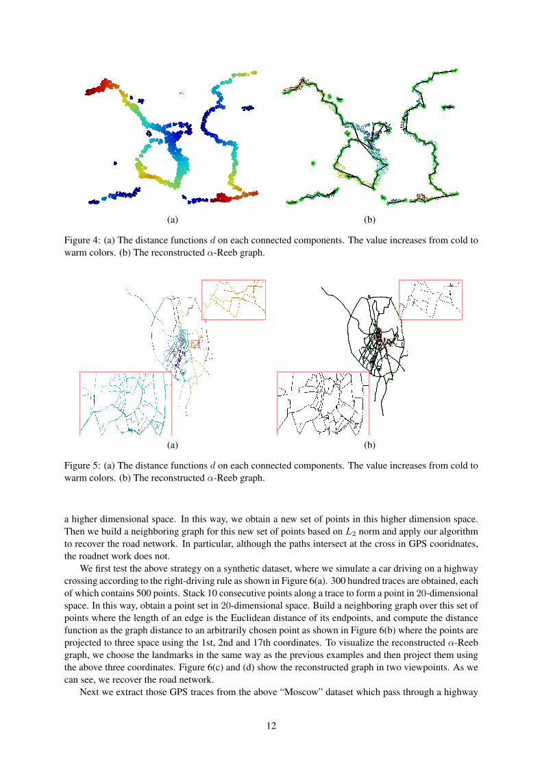
In this section, we apply our algorithm to a few data sets. The first data set is that of earthquake loca-tions through which we wish to learn the geometric information about earthquake faults. The raw datawas obtained from USGS Earthquake Search [32] and consists of earthquakes between 01/01/1970 and01/01/2010, of magnitude greater than 5.0, and of location in the rectangular area between latitudes -75degrees and 75 degrees and longitude between -170 degrees and 10 degrees. The raw earthquake dataset contains the coordinates of the epicenters of 12790 earthquakes. We follow the procedure describedin [1] to remove outliers and randomly sampled 1600 landmarks. Finally, we computed a neighboringgraph from these landmarks with parameter 4. The length of an edge in this graph is the Euclidean dis-tance between its endpoints. For each connected component, we fix a root point and compute the graphdistance function d to the root point as shown in Figure 4(a). Set α also equals 4 and apply our algorithmto the above data to obtain the α-Reeb graph. In general α-Reeb graph is an abstract metric graph. In thisexample, for the purpose of visualization, we use the coordinates of the landmarks to embed the graphinto the plane as follows. Recall that for a copy of interval Ik representing the node V l

k in G, we split

10

I4

I2

I1

I3

H14

H10

V 14

V 13

V 22V 1

2

V 10

I0

H12 H2

2

H13

H21

H11

V 21V 1

1

I4

I3

I2I2

I0

I1I1

H d I

G disjoint union ofcopies of intervals

α-Reeb graph

Figure 3: Illustration of the different steps of the algorithm for computing α-Reeb graph. In the disjointunion of copies of intervals, the subintervals marked with same labels are identified in the α-Reeb graph.

it into two by adding a point in the middle. We embed the endpoints of the interval to the landmarks ofthe minimum and the maximum of the funciton d in V l

k , and the point in the middle to the landmark ofthe median of the function d in V l

k . Figure 4(b) shows the embedding of the α-Reeb graph. Note thisembedding may introduce metric distortion, i.e., the Euclidean length of the edge may not reflect thelength of the corresponding edge in the α-Reeb graph.

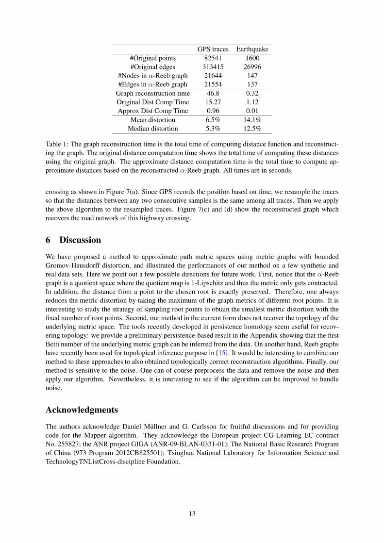
The second data set is that of 500 GPS traces tagged “Moscow” from OpenStreetMap [30]. Since carsmove on roads, we expect the locations of cars to provide information about the metric graph structureof the Moscow road network. We first selected a metric ε-net on the raw GPS locations with ε =0.0001 using furthest point sampling. Then, we computed a neighboring graph from the samples withparameter 0.0004. Again for each connected component, we fix a root point and compute the graphdistance function d to the root point as shown in Figure 5(a). Set α also equals 0.0004 and compute theα-Reeb graph. Again, we use the same method as above to embed the α-Reeb graph into the plane, asshown in Figure 5(b).

To evaluate the quality of our α-Reeb graph for each data set, we computed both original pairwisedistances, and pairwise distances approximated from the constructed α-Reeb graph. For GPS traces, werandomly select 100 points as the data set is too big to compute all pairwise distances. We also evaluatedthe use of α-Reeb graph to speed up distance computations by showing reductions in computation time.Only pairs of points in the same connected component are included because we obtain zero error forthe pairs of vertices that are not. Statistics for the size of the reconstructed graph, error of approximatedistances, and reduction in computation time are given in Table 1.

Road network is directional. There are one-way streets. In fact, roads are often split so that cars indifferent directions run in different lanes. In particular, this is the true for highways. In addition, whentwo roads cross in GPS coordinates, they may bypass through a tunnel or an evaluated bridge and thusthe road network itself may not cross. Since in most circumstances, drivers follow the road network anddo not drive against the traffic, such directional information is contained in the GPS traces. Here weencode the directional information by stacking several consecutive GPS coordinates to form a point in

11

(a) (b)

Figure 4: (a) The distance functions d on each connected components. The value increases from cold towarm colors. (b) The reconstructed α-Reeb graph.

(a) (b)

Figure 5: (a) The distance functions d on each connected components. The value increases from cold towarm colors. (b) The reconstructed α-Reeb graph.

a higher dimensional space. In this way, we obtain a new set of points in this higher dimension space.Then we build a neighboring graph for this new set of points based on L2 norm and apply our algorithmto recover the road network. In particular, although the paths intersect at the cross in GPS cooridnates,the roadnet work does not.

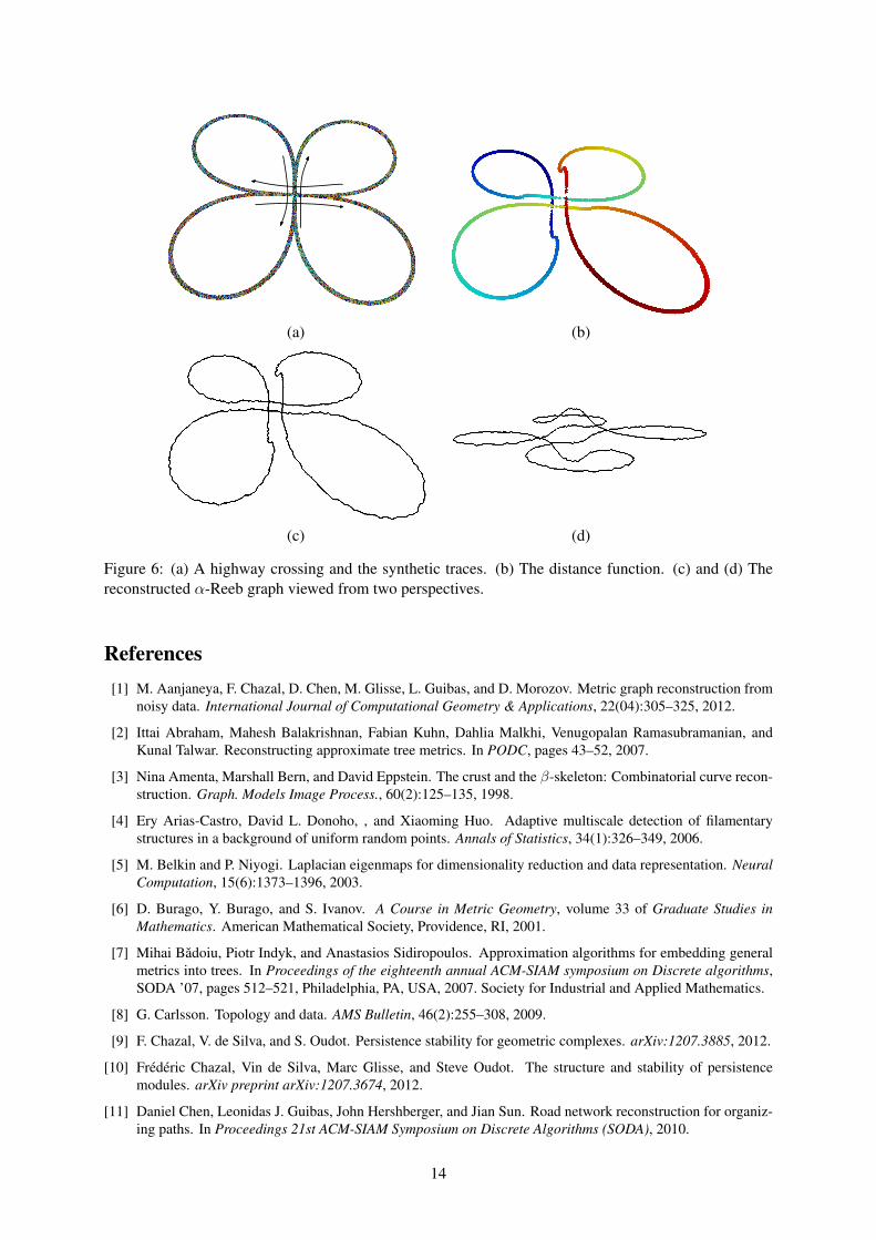
We first test the above strategy on a synthetic dataset, where we simulate a car driving on a highwaycrossing according to the right-driving rule as shown in Figure 6(a). 300 hundred traces are obtained, eachof which contains 500 points. Stack 10 consecutive points along a trace to form a point in 20-dimensionalspace. In this way, obtain a point set in 20-dimensional space. Build a neighboring graph over this set ofpoints where the length of an edge is the Euclidean distance of its endpoints, and compute the distancefunction as the graph distance to an arbitrarily chosen point as shown in Figure 6(b) where the points areprojected to three space using the 1st, 2nd and 17th coordinates. To visualize the reconstructed α-Reebgraph, we choose the landmarks in the same way as the previous examples and then project them usingthe above three coordinates. Figure 6(c) and (d) show the reconstructed graph in two viewpoints. As wecan see, we recover the road network.

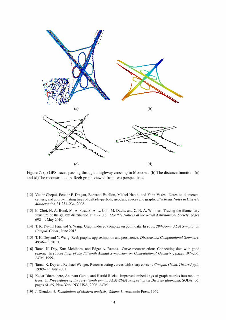
Next we extract those GPS traces from the above “Moscow” dataset which pass through a highway

12

GPS traces Earthquake#Original points 82541 1600#Original edges 313415 26996

#Nodes in α-Reeb graph 21644 147#Edges in α-Reeb graph 21554 137

Graph reconstruction time 46.8 0.32Original Dist Comp Time 15.27 1.12Approx Dist Comp Time 0.96 0.01

Mean distortion 6.5% 14.1%Median distortion 5.3% 12.5%

Table 1: The graph reconstruction time is the total time of computing distance function and reconstruct-ing the graph. The original distance computation time shows the total time of computing these distancesusing the original graph. The approximate distance computation time is the total time to compute ap-proximate distances based on the reconstructed α-Reeb graph. All times are in seconds.

crossing as shown in Figure 7(a). Since GPS records the position based on time, we resample the tracesso that the distances between any two consecutive samples is the same among all traces. Then we applythe above algorithm to the resampled traces. Figure 7(c) and (d) show the reconstructed graph whichrecovers the road network of this highway crossing.

6 Discussion

We have proposed a method to approximate path metric spaces using metric graphs with boundedGromov-Hausdorff distortion, and illustrated the performances of our method on a few synthetic andreal data sets. Here we point out a few possible directions for future work. First, notice that the α-Reebgraph is a quotient space where the quotient map is 1-Lipschitz and thus the metric only gets contracted.In addition, the distance from a point to the chosen root is exactly preserved. Therefore, one alwaysreduces the metric distortion by taking the maximum of the graph metrics of different root points. It isinteresting to study the strategy of sampling root points to obtain the smallest metric distortion with thefixed number of root points. Second, our method in the current form does not recover the topology of theunderlying metric space. The tools recently developed in persistence homology seem useful for recov-ering topology: we provide a preliminary persistence-based result in the Appendix showing that the firstBetti number of the underlying metric graph can be inferred from the data. On another hand, Reeb graphshave recently been used for topological inference purpose in [15]. It would be interesting to combine ourmethod to these approaches to also obtained topologically correct reconstruction algorithms. Finally, ourmethod is sensitive to the noise. One can of course preprocess the data and remove the noise and thenapply our algorithm. Nevertheless, it is interesting to see if the algorithm can be improved to handlenoise.

Acknowledgments

The authors acknowledge Daniel Mullner and G. Carlsson for fruitful discussions and for providingcode for the Mapper algorithm. They acknowledge the European project CG-Learning EC contractNo. 255827; the ANR project GIGA (ANR-09-BLAN-0331-01); The National Basic Research Programof China (973 Program 2012CB825501); Tsinghua National Laboratory for Information Science andTechnologyTNListCross-discipline Foundation.

13

(a) (b)

(c) (d)

Figure 6: (a) A highway crossing and the synthetic traces. (b) The distance function. (c) and (d) Thereconstructed α-Reeb graph viewed from two perspectives.

References[1] M. Aanjaneya, F. Chazal, D. Chen, M. Glisse, L. Guibas, and D. Morozov. Metric graph reconstruction from

noisy data. International Journal of Computational Geometry & Applications, 22(04):305–325, 2012.

[2] Ittai Abraham, Mahesh Balakrishnan, Fabian Kuhn, Dahlia Malkhi, Venugopalan Ramasubramanian, andKunal Talwar. Reconstructing approximate tree metrics. In PODC, pages 43–52, 2007.

[3] Nina Amenta, Marshall Bern, and David Eppstein. The crust and the β-skeleton: Combinatorial curve recon-struction. Graph. Models Image Process., 60(2):125–135, 1998.

[4] Ery Arias-Castro, David L. Donoho, , and Xiaoming Huo. Adaptive multiscale detection of filamentarystructures in a background of uniform random points. Annals of Statistics, 34(1):326–349, 2006.

[5] M. Belkin and P. Niyogi. Laplacian eigenmaps for dimensionality reduction and data representation. NeuralComputation, 15(6):1373–1396, 2003.

[6] D. Burago, Y. Burago, and S. Ivanov. A Course in Metric Geometry, volume 33 of Graduate Studies inMathematics. American Mathematical Society, Providence, RI, 2001.

[7] Mihai Badoiu, Piotr Indyk, and Anastasios Sidiropoulos. Approximation algorithms for embedding generalmetrics into trees. In Proceedings of the eighteenth annual ACM-SIAM symposium on Discrete algorithms,SODA ’07, pages 512–521, Philadelphia, PA, USA, 2007. Society for Industrial and Applied Mathematics.

[8] G. Carlsson. Topology and data. AMS Bulletin, 46(2):255–308, 2009.

[9] F. Chazal, V. de Silva, and S. Oudot. Persistence stability for geometric complexes. arXiv:1207.3885, 2012.

[10] Frederic Chazal, Vin de Silva, Marc Glisse, and Steve Oudot. The structure and stability of persistencemodules. arXiv preprint arXiv:1207.3674, 2012.

[11] Daniel Chen, Leonidas J. Guibas, John Hershberger, and Jian Sun. Road network reconstruction for organiz-ing paths. In Proceedings 21st ACM-SIAM Symposium on Discrete Algorithms (SODA), 2010.

14

(a) (b)

(c) (d)

Figure 7: (a) GPS traces passing through a highway crossing in Moscow . (b) The distance function. (c)and (d)The reconstructed α-Reeb graph viewed from two perspectives.

[12] Victor Chepoi, Feodor F. Dragan, Bertrand Estellon, Michel Habib, and Yann Vaxes. Notes on diameters,centers, and approximating trees of delta-hyperbolic geodesic spaces and graphs. Electronic Notes in DiscreteMathematics, 31:231–234, 2008.

[13] E. Choi, N. A. Bond, M. A. Strauss, A. L. Coil, M. Davis, and C. N. A. Willmer. Tracing the filamentarystructure of the galaxy distribution at z ∼ 0.8. Monthly Notices of the Royal Astronomical Society, pages692–+, May 2010.

[14] T. K. Dey, F. Fan, and Y. Wang. Graph induced complex on point data. In Proc. 29th Annu. ACM Sympos. onComput. Geom., June 2013.

[15] T. K. Dey and Y. Wang. Reeb graphs: approximation and persistence. Discrete and Computational Geometry,49:46–73, 2013.

[16] Tamal K. Dey, Kurt Mehlhorn, and Edgar A. Ramos. Curve reconstruction: Connecting dots with goodreason. In Proceedings of the Fifteenth Annual Symposium on Computational Geometry, pages 197–206.ACM, 1999.

[17] Tamal K. Dey and Rephael Wenger. Reconstructing curves with sharp corners. Comput. Geom. Theory Appl.,19:89–99, July 2001.

[18] Kedar Dhamdhere, Anupam Gupta, and Harald Racke. Improved embeddings of graph metrics into randomtrees. In Proceedings of the seventeenth annual ACM-SIAM symposium on Discrete algorithm, SODA ’06,pages 61–69, New York, NY, USA, 2006. ACM.

[19] J. Dieudonne. Foundations of Modern analysis, Volume 1. Academic Press, 1969.

15

[20] H. Edelsbrunner and J. Harer. Computational Topology: an Introduction. American Mathematical Society,Providence, RI, 2010.

[21] H. Edelsbrunner, D. Letscher, and A. Zomorodian. Topological persistence and simplification. DiscreteComput. Geom., 28:511–533, 2002.

[22] Jittat Fakcharoenphol, Satish Rao, and Kunal Talwar. A tight bound on approximating arbitrary metrics bytree metrics. In Proceedings of the thirty-fifth annual ACM symposium on Theory of computing, STOC ’03,pages 448–455, New York, NY, USA, 2003. ACM.

[23] C. R. Genovese, M. Perone-Pacifico, I. Verdinelli, and L. Wasserman. The Geometry of NonparametricFilament Estimation. J. Amer. Statist. Assoc., (107):788–799, 2012.

[24] Christopher R. Genovese, Marco Perone-Pacifico, Isabella Verdinelli, and Larry Wasserman. On the pathdensity of a gradient field. Annals of Statistics, 37(6A):3236–3271, 2009.

[25] Christopher R. Genovese, Marco Perone-Pacifico, Isabella Verdinelli, and Larry Wasserman. Nonparametricridge estimation. arXiv:1212.5156, 2012.

[26] M. Gromov. Metric Structures for Riemannian and Non-Riemannian Spaces. Birkhauser, 2nd edition, 2007.

[27] William Harvey, Yusu Wang, and Rephael Wenger. A randomized o(m log m) time algorithm for computingreeb graph of arbitrary simplicial complexes. In Proc. 26th Annu. ACM Sympos. on Comput. Geom., 2010.

[28] J.C. Haussmann. On the vietoris-rips complexes and a cohomology theory fo metric spaces. Ann. of Math.Stud., 138:175–188, 1995.

[29] S. Lafon. Diffusion Maps and Geodesic Harmonics. PhD. Thesis, Yale University, 2004.

[30] Openstreetmap. http://www.openstreetmap.org/.

[31] Salman Parsa. A deterministic o(m log m) time algorithm for the reeb graph. In Proceedings of the 2012symposuim on Computational Geometry, SoCG ’12, pages 269–276, New York, NY, USA, 2012. ACM.

[32] Earthquake search. http://earthquake.usgs.gov/earthquakes/eqarchives/epic/.

[33] G. Singh, F. Memoli, and G. Carlsson. Topological methods for the analysis of high dimensional data setsand 3d object recognition. In Eurographics Symposium on Point-Based Graphics, 2007.

[34] J. B. Tenenbaum, V. De Silva, and J. C. Langford. A global geometric framework for nonlinear dimensionalityreduction. Science, 2000.

[35] F. Tupin, H. Maitre, Mangin, Nicolas J.-F., J.-M., and E. Pechersky. Detection of linear features in SARimages: Application to road network extraction. IEEE Transactions on Geoscience and Remote Sensing,36:434–453, 1998.

[36] A. Zomorodian and G. Carlsson. Computing persistent homology. Discrete Comput. Geom., 33(2):249–274,2005.

Appendix

Getting the first Betti number of a graph from an approximation

Although our metric graph reconstruction algorithm does not provide topological guarantees, we showbelow that, using persistent topology arguments, that the first Betti number of a graph can be inferredfrom an approximation.

Recall that given a compact metric space (X, dX) and a real parameter α > 0, the Vietoris-Ripscomplex Rips(X,α) is the simplicial complex with vertex set X and whose simplices are the finitesubsets of X with diameter at most α:

σ = [x0, x1, · · · , xk] ∈ Rips(X,α)⇔ dX(xi, xj) 6 α forall i, j.

16

Lemma 6.1. Let G be a connected metric graph and let l(G) be the length of the shortest loop inG that is not homologous to 0. For any metric space D such that dGH(G,D) < 1

16 l(G) and anydGH(G,D) < α < 3

16 l(G), the first Betti number of G is given by

b1(G) = rank (H1(Rips(D,α))→ H1(Rips(D, 3α))

where the homomorphism between the homology groups is the one induced by the inclusion maps betweenthe Rips complexes.

Proof. The proof follows from a result of [28] that relates the homology of the Rips complexes builton top of G to the homology of G and a result of [9] that allows to relate the Rips filtration built ontop of G and D at the homology level. Since G is a geodesic path, it follows from Theorem 3.5 andRemark 2), p.179 in [28] that for any α < 1

4 l(G), Rips(G,α) and G are homotopy equivalent. More-over, from Proposition 3.3 in [28], for any α 6 α′ < 1

4 l(G), the homomorphism H1(Rips(G,α)) →H1(Rips(G,α′)) induced by the inclusion map is an isomorphism.

Now let C ⊂ D×G be an ε-correspondence betweenD andG where ε < 116 l(G). According to [9],

the persistence modules (H1(Rips(D,α))α∈R+ and (H1(Rips(G,α))α∈R+ are ε-interleaved. Now let αbe as in the statement of the lemma and let β > 0 be such that β+ ε < α. The ε-interleaving induces thefollowing sequence of homomorphisms

H1(Rips(G, β))→ H1(Rips(D,α))→ H1(Rips(G,α+ε))→ H1(Rips(D, 3α))→ H1(Rips(G, 3α+ε))

where the composition of two consecutive homomorphisms is the homomorphism induced by the inclu-sion map between the corresponding Rips complexes. As a consequence since 3α+ε < 1

4 l(G) the homo-morphisms H1(Rips(G, β))→ H1(Rips(G,α+ ε)) and H1(Rips(G,α+ ε))→ H1(Rips(G, 3α+ ε))are isomorphisms of rank b1(G). It follows that the rank of H1(Rips(D,α)) → H1(Rips(D, 3α)) isequal to b1(G).

17