group ica/iva of fmri toolbox (gift) manual -...
TRANSCRIPT
Group ICA/IVA Of fMRI Toolbox
Group ICA/IVA of fMRI Toolbox (GIFT) Manual The GIFT Documentation Team
Feb 23, 2017

Group ICA/IVA Of fMRI Toolbox
1 TABLE OF CONTENTS
2 Introduction ........................................................................................................................................................5
2.1 What is GIFT? ..............................................................................................................................................5
2.2 Why ICA On fMRI data? ..............................................................................................................................5
2.3 Why Group ICA? .........................................................................................................................................5
3 Getting Started With GIFT ..................................................................................................................................8
3.1 Installing GIFT .............................................................................................................................................8
3.2 Installing Example Subjects ........................................................................................................................8
3.3 HTML Help Manual .....................................................................................................................................8
3.4 New Features ..............................................................................................................................................8
3.5 GIFT Updates ..............................................................................................................................................9
3.6 Things to do before configuring the analysis .............................................................................................9
3.6.1 Compiling MEX files ............................................................................................................................9
3.6.2 Memory Requirements ................................................................................................................... 10
3.6.3 Organizing data ................................................................................................................................ 10
3.6.4 Defaults ............................................................................................................................................ 10
3.7 Spatial Templates .................................................................................................................................... 11
3.8 Menus ...................................................................................................................................................... 12
3.9 Analysis Functions ................................................................................................................................... 15
3.9.1 Setup ICA Analysis........................................................................................................................... 15
3.9.2 Run Analysis ..................................................................................................................................... 24
3.9.3 Analysis Info ..................................................................................................................................... 26
3.10 Visualization methods ............................................................................................................................. 28
3.10.1 Display GUI ...................................................................................................................................... 28
3.10.2 Subject Component Explorer ........................................................................................................... 31
3.10.3 Orthogonal Explorer ........................................................................................................................ 33
3.10.4 Composite Viewer ........................................................................................................................... 33
3.11 Sorting Components ................................................................................................................................ 35
3.11.1 Temporal Sorting ............................................................................................................................. 35
3.11.2 Spatial Sorting .................................................................................................................................. 40
3.12 Utilities ..................................................................................................................................................... 43
3.12.1 Generate Mask ................................................................................................................................ 44
3.12.2 Remove Component (s) ................................................................................................................... 45
3.12.3 Temporal Sorting ............................................................................................................................. 47

Group ICA/IVA Of fMRI Toolbox
3.12.4 Stats On Beta Weights ..................................................................................................................... 48
3.12.5 SPM Stats ......................................................................................................................................... 50
3.12.6 Spatial-temporal Regression ........................................................................................................... 50
3.12.7 Write Taliarach Table ....................................................................................................................... 50
3.12.8 Component Labeler ......................................................................................................................... 50
3.12.9 Ascii To SPM.mat ............................................................................................................................. 51
3.12.10 Event Average .............................................................................................................................. 52
3.12.11 Calculate Stats ............................................................................................................................. 52
3.12.12 Spectral Group Compare ............................................................................................................. 52
3.12.13 Single Trial Amplitudes ................................................................................................................ 53
3.12.14 Z-shift ........................................................................................................................................... 54
3.12.15 Percent Variance ......................................................................................................................... 54
3.13 Toolboxes ................................................................................................................................................ 55
3.13.1 ICASSO ............................................................................................................................................. 55
3.13.2 Mancovan ........................................................................................................................................ 57
3.13.3 Temporal dFNC ................................................................................................................................ 72
3.13.4 Spatial dFNC ..................................................................................................................................... 80
3.13.5 Noise cloud ...................................................................................................................................... 84
3.14 Batch Script .............................................................................................................................................. 85
3.14.1 Analysis ............................................................................................................................................ 85
3.14.2 Display ............................................................................................................................................. 89
3.14.3 Stats On Beta Weights ..................................................................................................................... 90
3.14.4 Mancovan ........................................................................................................................................ 92
3.14.5 Temporal dFNC ................................................................................................................................ 92
3.15 GICA Command line ................................................................................................................................. 93
3.16 Output files naming ................................................................................................................................. 93
3.17 Source Based Morphometry.................................................................................................................... 94
3.17.1 SBM Stats ......................................................................................................................................... 95
3.18 Independent Vector Analysis................................................................................................................... 96
3.19 Display Tools ............................................................................................................................................ 98
3.19.1 Image Viewer ................................................................................................................................... 98
3.19.2 Component Viewer ........................................................................................................................ 101
3.19.3 Network Summary ......................................................................................................................... 102
4 Process Involved In Group ICA....................................................................................................................... 106
4.1 Data Reduction (PCA) ............................................................................................................................ 106
Group ICA/IVA Of fMRI Toolbox
4.2 Independent Component analysis ......................................................................................................... 106
4.2.1 Infomax .......................................................................................................................................... 107
4.2.2 Fast ICA .......................................................................................................................................... 107
4.2.3 JADE OPAC ..................................................................................................................................... 107
4.2.4 SIMBEC ........................................................................................................................................... 108
4.2.5 AMUSE ........................................................................................................................................... 108
4.2.6 ERICA ............................................................................................................................................. 108
4.2.7 EVD ................................................................................................................................................ 108
4.2.8 Constrained ICA (Spatial) ............................................................................................................... 108
4.2.9 GIG-ICA .......................................................................................................................................... 109
4.2.10 Real-valued ICA-EBM ..................................................................................................................... 109
4.2.11 Real-valued ICA-ERBM ................................................................................................................... 109
4.3 Back-reconstruction .............................................................................................................................. 109
4.4 Scaling Components .............................................................................................................................. 109
4.5 Group Stats ............................................................................................................................................ 110
5 Bibliography ................................................................................................................................................... 110
6 Appendix ........................................................................................................................................................ 113
6.1 Experimental Paradigms ........................................................................................................................ 113
6.2 Defaults.................................................................................................................................................. 113
6.3 Options Window .................................................................................................................................... 116
6.4 Defaults GUI ........................................................................................................................................... 118
6.5 Regular Expressions ............................................................................................................................... 118
6.6 Interactive Figure Window .................................................................................................................... 119
6.7 GIFT Startup ........................................................................................................................................... 120

Group ICA/IVA Of fMRI Toolbox
2 INTRODUCTION
This manual is divided mainly into three chapters. Motivation for using the group ICA of fMRI Toolbox (GIFT) is discussed in this chapter. In Chapter 3, quick start to the toolbox is discussed. Chapter 4 focusses on the process involved in group ICA. In Section 3.17, Source Based Morphometry is discussed. A brief discussion is given on Independent Vector Analysis (IVA) in Section 3.18.
2.1 WHAT IS GIFT?
GIFT is an application developed in MATLAB that enables group inferences from fMRI data using Independent Component Analysis (ICA). A detailed explanation of ICA is explained in the next section. GIFT is used to run both single subject and single session analysis as well as group analysis. Toolbox is thoroughly tested and works on MATLAB R2008a and higher.
2.2 WHY ICA ON FMRI DATA?
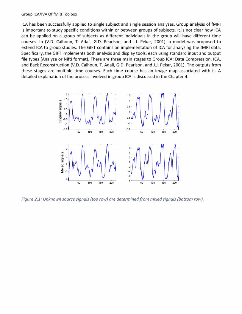
Functional Magnetic Resonance Imaging (fMRI) is a modality for studying the brain function. fMRI techniques use Blood Oxygenation Level Dependent (BOLD) signal as a measure for detecting the neural activity. Since fMRI uses an indirect measure of neural activity, mathematical models are needed to analyze the data. Many fMRI experiments use a block design in which the subject is instructed to perform experimental and control tasks in an alternating sequence of 20-40 second blocks. The resulting activity is recorded for each volume element (voxel) of the brain. Based on events of the experimental task and knowing shape of the haemodynamic response, a reference function is constructed. Model based techniques such as SPM (Statistical Parameteric Mapping, 1991) use this reference function to separate the signals of interest and the signals not of interest. A general method is necessary which does not depend on the prior information of the experiment or task. In this respect, a statistical technique called Independent Component Analysis (ICA) (M. J. McKneown, Scott Makeig, Greg G. Brown, Tzyy-Ping Jung, Sandra S. Kindermann, Anthony J. Bell and Terrence J. Sejnowski, 1998) is proposed that allows the extraction of signals of interest and not of interest without any prior information about the task. Thus ICA analysis could reveal characteristics of the brain function that cannot be modeled due to lack of prior information. Independent Component Analysis (ICA) is a method of blind source signal separation i.e., ICA allows one to extract or “unmix” unknown source signals which are linearly mixed together (Figure 2.1). For fMRI data, temporal and spatial ICA are possible, but spatial ICA is by far the most common approach. The GIFT implements spatial ICA of fMRI data. In the current version, option is provided to do temporal ICA. In spatial ICA, spatially independent brain sources or components are calculated from fMRI data. Figure 2.2 shows a component extracted from the fMRI data. For a complete description of this experiment please see Appendix 6.1.
2.3 WHY GROUP ICA?
Group ICA/IVA Of fMRI Toolbox
ICA has been successfully applied to single subject and single session analyses. Group analysis of fMRI is important to study specific conditions within or between groups of subjects. It is not clear how ICA can be applied on a group of subjects as different individuals in the group will have different time courses. In (V.D. Calhoun, T. Adali, G.D. Pearlson, and J.J. Pekar, 2001), a model was proposed to extend ICA to group studies. The GIFT contains an implementation of ICA for analyzing the fMRI data. Specifically, the GIFT implements both analysis and display tools, each using standard input and output file types (Analyze or Nifti format). There are three main stages to Group ICA; Data Compression, ICA, and Back Reconstruction (V.D. Calhoun, T. Adali, G.D. Pearlson, and J.J. Pekar, 2001). The outputs from these stages are multiple time courses. Each time course has an image map associated with it. A detailed explanation of the process involved in group ICA is discussed in the Chapter 4.
Figure 2.1: Unknown source signals (top row) are determined from mixed signals (bottom row).

Group ICA/IVA Of fMRI Toolbox
Figure 2.2: A component consists of a spatial map and a timecourse

Group ICA/IVA Of fMRI Toolbox
3 GETTING STARTED WITH GIFT
The source code and the example subjects fMRI data need to be installed. These are available on project web page (http://mialab.mrn.org/software/gift/index.html). Also available on this web page are posters on GIFT at the conferences like Society of Biological Psychiatry and Human Brain Mapping. The mailing list is: [email protected]. Please send comments and bug reports to: [email protected] or [email protected].
3.1 INSTALLING GIFT
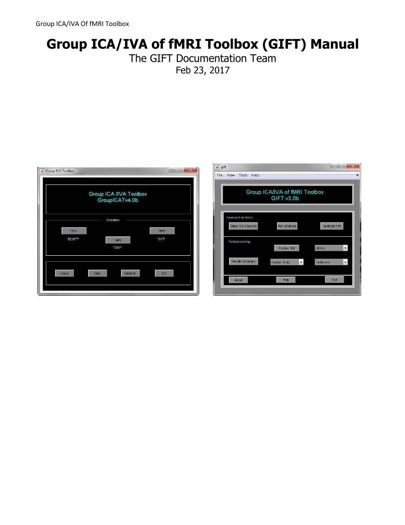
Unzip the file GroupICATv4.0b.zip and copy the folder GroupICATv4.0b onto your local machine. Add GIFT directories to the MATLAB search path or run the gift.m file to automatically add GIFT directories. The GIFT path by default will be set at the bottom of the MATLAB path. You can create gift_startup.m (Appendix 6.7) file for setting the path according to your needs. After the GIFT path is set, GIFT toolbox (Figure 3.2) opens in a new figure window. There is also an option to run group ICA using a batch script (Section 3.14.1). Batch script is very useful for running large data-sets. Note:
GIFT toolbox can also be invoked by using the statement groupica and clicking on the fMRI button (Figure 3.1) or by typing groupica fmri at the MATLAB command window.
If you have downloaded an older version of GIFT, make sure that there is only one version on path at a time.
3.2 INSTALLING EXAMPLE SUBJECTS Download the example_subjects.zip file and unzip into an appropriate directory. Included in this file are three subjects pre-processed fMRI data from a visuomotor task (See (V.D. Calhoun, T. Adali, G.D. Pearlson, and J.J. Pekar, 2001) for a complete description of the task). Whole brain and single slice data (for rapid testing) are provided. More information on the task the subject performed while in the scanner is given in the Appendix 6.1. Each example subject also contains a functional data-set, which contains only one brain slice. If you are having problems with this toolbox you may test this with a smaller data-set.
3.3 HTML HELP MANUAL When you click Help button (Figure 3.2), HTML help manual is opened in the default web browser. ”GIFT-help” menu is plotted on some figures which will directly open a particular topic.
3.4 NEW FEATURES

Group ICA/IVA Of fMRI Toolbox
1) A subject outlier detection tool is now added as a “Generate Mask” utility in the GIFT toolbox. An average mask is generated and subjects below a certain correlation threshold are excluded from the analysis. At the end of the mask generation, a GIFT batch file is created which can be used to run the group ICA.
2) An option is now provided to generate results summary in the Mancovan toolbox. This tool can be accessed using “display” button in the Mancovan toolbox. Univariate results are plotted in a separate figure for each significant covariate and a connectogram display (Rashid, B., et al. (2014), “Dynamic connectivity states estimated from resting fMRI Identify differences among Schizophrenia, bipolar disorder, and healthy control subjects”, Frontiers in human neuroscience) is used to show the FNC plots.
3) We now provide an option in the Mancovan toolbox to run univariate tests using the selected covariates bypassing the multivariate tests. This tool can be accessed using “Run analysis” button in the Mancovan toolbox.
4) The “Group networks” tool is renamed to a more general “network summary” in the GIFT display tools. The network summary display uses the component network information and optional FNC information to generate composite orthogonal views (Damaraju, E., et al. (2014), “Dynamic functional connectivity analysis reveals transient states of dysconnectivity in schizophrenia", NeuroImage), composite rendered surfaces of brain, stacked orthogonal slices, FNC matrix viewer and connectogram FNC plot.
5) We now provide an option to use the temporal design matrix information in the “Results Summary” button to compute R2 and one sample t-test on beta weights in the GIFT toolbox. This tool can also be accessed as temporal sorting under “Utilities” drop down box.
6) The stand-alone image viewer tool is now enabled to select multiple component images which can be plotted independently or in a composite plot (montage, render or orthogonal slices).
7) An option is now provided to export results to PDF or HTML file in the component viewer display tool.
8) MOO-ICAR algorithm name is changed to GIG-ICA.
3.5 GIFT UPDATES
We post the updates to the software that contain new features or any bug fixes in the updates section of the project web page (http://mialab.mrn.org/software/gift/index.html). Please see Updates_Readme.txt in updates webpage for more details.
3.6 THINGS TO DO BEFORE CONFIGURING THE ANALYSIS
3.6.1 Compiling MEX files
SPM MEX binaries - We use SPM8 volume functions to read and write image data.
Group ICA MEX binaries - C-MEX files are provided for computing the eigen values of a symmetric matrix. The compiled MEX binaries are used only when you select packed storage scheme for computing covariance matrix.
Group ICA/IVA Of fMRI Toolbox
GLASSO - FORTRAN MEX file (GLASSO, 2007) is provided for estimating a sparse inverse covariance matrix using a L1 penalty when using temporal dFNC toolbox.
To compile the MEX source code, type icatb_compile_mex_files at the MATLAB command prompt. Please see below to copy the SPM MEX binaries manually if the source code fails to compile:
Copy SPM8 MEX binaries like spm_bwlabel*, spm_existfile*, spm_sample_vol*, spm_slice_vol* to the directory icatb\icatb_spm8_files and prefix them with icatb_.
Copy SPM8 MEX binaries like spm8\@file_array\private\* to icatb_spm8_files\@icatb_file_array\private and prefix them with icatb_.
Note: * refers to the MEX file extension on your Operating System. Type mexext on the MATLAB command window to get the MEX file extension on the Operating System you are working on.
3.6.2 Memory Requirements Since PCA and ICA are multivariate approaches unlike General Linear Model, there are some memory requirements to do the group ICA/IVA analysis. We added a script icatb_mem_ica.m which will give a close estimate of RAM required to do the group ICA/IVA analysis. Please enter the parameters like number of voxels, time points, subjects, sessions, components and reduction steps in the input parameters section of the script and run the script to get an approximate amount of RAM required in gigabytes.
3.6.3 Organizing data Organizing data reduces the amount of selection. GIFT has two ways to enter the data for GUI and four ways to enter the data using the batch script.
First method requires the data to be in one root folder with a common file pattern (like sw*.img) for all subjects and sessions. Each subject folder can have session folders and the number of session folders with the matching file pattern should be the same over subjects.
Second method does not require the data to be in one root folder or have a common file pattern but the selection process through GUI can be tedious for large data-sets and therefore batch script (Section 3.14.1) is recommended.
Third method uses regular expressions to get the subject and session directories. This option is useful in matching directories that have nested paths. However, this option still requires a common file pattern for all the subjects. Please see Section 3.14.1 for more information.
Option is provided to paste the file names in the fourth method (Section 3.14.1).
3.6.4 Defaults Defaults are stored in icatb_defaults.m file. You could also change these defaults from the GUI (Appendix 6.4). Configure the specified defaults before using setup ICA as needed.
FUNCTIONAL_DATA_FILTER - Set the variable to *.nii if you would like to write components as 4D Nifti files.
ZIP_IMAGE_FILES - By default, components will be compressed in zip format. If you want to turn off the compression, set variable value to ’no’. Uncompressed data is faster to load in memory.
SPM_STATS_WRITE_TAL - If you plan to do one sample t-tests on components over subjects using SPM5, SPM8 or SPM12, set variable value to 1.

Group ICA/IVA Of fMRI Toolbox
CENTER_IMAGES - By default, subject component spatial maps after the scaling components step is centered based on the skewness of the distribution of the mean component maps. If you want to turn off this option, set the variable to 0.
MAX_AVAILABLE_RAM - This variable is used during the run analysis step and best PCA settings for each option (maximize performance or less memory usage) are used. Set this variable value to the maximum available RAM.
WRITE_ANALYSIS_STEPS_IN_DIRS - Organize analysis results in directories. When this variable is set to 1, analysis steps are saved in separate directories. The directories naming are as follows:
o Data reduction files are stored in *_data_reduction_files o ICA files are stored in *_ica_files o Back-reconstruction files are stored in *_back_reconstruction_files o Scaled components are stored in *_scaling_components_files o Group stats are stored in *_group_stats_files
CONSERVE_DISK_SPACE - Set the variable value as needed. The following are the options: o 0 - Analysis runs faster with this option. All the intermediate analysis files are written. o 1 - Only the required analysis files are written which will be used during the post-processing
(display, components sorting, remove components, etc). o 2 - All the intermediate analysis files (Data reduction, back-reconstruction, scaled components
MAT files) are cleaned up after the end of the group stats step. Only the basic post-processing steps like display and components sorting will work with this option.
DEFAULT_MASK_OPTION - By default, first file of each subject is used to generate the default mask. If you want to use all files, set the variable value to ‘all_files’.
REMOVE_CONSTANT_VOXELS - Constant voxels are removed in the fMRI data when this variable is set to 1.
DEFAULT_MASK_SBM_MULTIPLIER - Default mask multiplier in SBM. Defaults is 1% of mean i.e., voxels greater than or equal to 1% of mean will be used.
EXPERIMENTAL_TR – Specify experimental TR in seconds. This information is used when computing spectra, filtering and despiking.
USE_UNIFORM_COLOR_COMPOSITE – By default, composite plots in the network summary and image viewer are shown as intensity maps. You have the option to use uniform colors when you set a value of 1 in the “USE_UNIFORM_COLOR_COMPOSITE” variable.
CONNECTOGRAM_SM_WIDTH – By default, the size of the connectogram spatial maps is automatically determined. If the thumbnails are too small, you could set a specified value like 0.06.
3.7 SPATIAL TEMPLATES
The following example spatial templates are provided in icatb\icatb_templates:
ref_right_visuomotor.nii - Mask containing the right visual regions.
ref_left_visuomotor.nii - Mask containing the left visual regions.
ref_default_mode.nii - Mask containing the default mode network regions. Please see (A. R. Franco, A. Pritchard, V. D. Calhoun, A. R Mayer, 2009) for more information.
*DMN_ICA_REST*.nii - This mask was created from a data-set of 42 subjects. During a fMRI scan, subjects were asked to relax and passively stare at a fixation cross. A pooled group ICA was performed and the default mode component network was selected to create this mask. We provide templates like rDMN_ICA_REST_3x3x3.nii and rDMN_ICA_REST_3x3x4.nii in the GIFT. Please see (A. R. Franco, A. Pritchard, V. D. Calhoun, A. R Mayer, 2009) for more information.

Group ICA/IVA Of fMRI Toolbox
*DMN_MASK.WFU*.nii - This mask was constructed using the Wake Forest Pick atlas toolbox. A binary mask was created by selecting the anatomical regions that have been most commonly reported to comprise the default mode network. The labels from the Wake Forest Atlas that constituted this mask included posterior cingulate (BAs 23/31), inferior and superior parietal lobes (BAs 7/39/40), superior frontal gyrus (BAs 8/9/10), and anterior cingulate cortex (BAs 11/32). In addition, a larger weight was given to the anterior and posterior cingulate cortex, which are believed to be the central nodes of the default mode network. A higher correlation was observed when giving a higher weight to these two central nodes. We provide templates like rDMN_MASK.WFU.3x3x3.nii and rDMN_MASK.WFU.3x3x4.nii in the GIFT. Please see (A. R. Franco, A. Pritchard, V. D. Calhoun, A. R Mayer, 2009) for more information.
3.8 MENUS
Menus are provided as a shortcut to the user-interface controls in the GIFT toolbox (Figure 3.2). The function of each menu is given below:
File o New - Setup ICA GUI will open after you have selected the output directory. o Open - Setup ICA GUI will open showing the values for the parameters after you have
selected the subject file that has suffix Subject.mat. o Close - Closes the GIFT Toolbox and the figures generated by the GIFT.
View o Analysis Info - Analysis information will be shown after you have selected the parameter
file that has suffix ica_parameter_info.mat.
Tools o Run Analysis - Analysis will be run after you have selected the parameter file. o Display GUI - Display GUI will be opened after you have selected the parameter file. o Utilities
Generate mask – Please see Section 3.12.1. Batch – This option runs multiple batch analyses. More information on input file
required for batch analysis is provided in Section 3.14.1. Remove component (s) - Removes a component or components from the data
after you have selected the parameter file. Please see Section 3.12.1 for more information.
Ascii_to_spm.mat - Creates SPM.mat from ascii file (containing regressor time courses) that is needed during temporal sorting. Please see Section 3.12.9 for more information.
Event Average - Event average is calculated for the ICA time courses. Please see Section 3.12.10 for more information.
Calculate Stats - Mean, standard deviation, t-maps are calculated for components over sessions, subjects or subjects and sessions.
Spectral Group Compare - This utility is used to compare the power spectra between groups. Please see Section 3.12.12 for more information.

Group ICA/IVA Of fMRI Toolbox
Temporal Sorting – Stand-alone tool is now provided to do multiple linear regression on ICA timecourses and model timecourses (Section 3.12.3).
Stats on beta weights - This utility is used to do one sample t-test or two sample t-test on the component images. Please see Section 3.12.3 for more information.
SPM Stats - Group statistics are computed on individual subject component maps using SPM toolbox. We integrated option to do t-tests using SPM in the GIFT toolbox.
Spatial-temporal regression - Given a set of GLM or ICA spatial maps and the original data of the subjects, you could use this utility to back reconstruct subject components (Section 3.12.6).
Write talairach table - Talairach daemon client is used to generate the talairach tables for the selected image. Please see Section 3.12.7 for more information.
Single trial amplitudes - We provide the option for calculating single trial amplitudes (Section 3.12.13) in GIFT.
Z-shift - Please see Section 3.12.14 for more information. Percent variance – Variance explained by the components in the data is
determined. Please see Section 3.12.15 for more information. o Display Tools
Image viewer - Options to do image rendering and displaying images as a montage or orthogonal slices are provided. We now provide options to do composite plots if multiple images are selected.
Component explorer - Standalone tool to display component maps and timecourses.
Composite viewer - Multiple components could be displayed as a composite map.
Orthogonal viewer - Component timecourse and orthogonal slices of components are shown. Also, BOLD timecourse is plotted for the selected voxel.
Component viewer - Mean and standard error mean of spectra is shown. Also orthogonal slices are plotted at the maximum voxel.
Network summary – This tool uses network information and corresponding components to generate composite orthogonal plots, rendered surface plots, stacked orthogonal slices, FNC matrix viewer and connectogram plots.
o Toolboxes ICASSO – ICA is run several times and best stable run estimates are used to
reconstruct individual subject components. Mancovan - Mancovan toolbox works on the ICA output. Multivariate stats is
used to determine the significant covariates which will be used later in the univariate tests. Please see 3.13.2 for more information.
Temporal dFNC - Dynamic FNC (dFNC) toolbox is used to study functional network connectivity dynamics. dFNC toolbox is based on paper (E. Allen, E. Damaraju, S. M. Plis, E. Erhardt, T. Eichele, and V. D.Calhoun, 2012). Please see 3.14.5 for using the toolbox.
Spatial dFNC – Dynamic FNC is computed in space using the mutual information between component maps. Please see Section 3.13.4 for more information.
o Results summary - Results are summarized using HTML or PDF report. Report includes ICASSO plots, components (maps, timecourses and spectra), statistics on beta weights

Group ICA/IVA Of fMRI Toolbox
obtained from temporal sorting, kurtosis values of components, FNC correlations and FNC values of spatial maps. To get accurate values for spectra, you need to set EXPERIMENTAL_TR in icatb_defaults.m for your experiment before doing group ICA.
Figure 3.1: Group ICA/IVA Toolbox

Group ICA/IVA Of fMRI Toolbox
Figure 3.2: GIFT Toolbox
3.9 ANALYSIS FUNCTIONS
3.9.1 Setup ICA Analysis
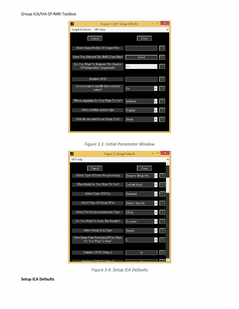
When you click Setup ICA button (Figure 3.2), Setup ICA GUI (Figure 3.3) will open after you have selected the output directory for the analysis. Setup ICA is the GUI used for entering parameters required for group ICA.
Figure 3.3 shows the main user interface controls. Some of the parameters are plotted in ”Setup ICA-Defaults”
menu (Figure 3.4). It is recommended that after entering the parameters in the main figure window parameters plotted in menu be changed. The parameters are explained below: Main User Interface Controls
Enter Name (Prefix) Of Output Files’ is the prefix string to all the output files created by GIFT. This should be a valid character name as the files will be saved using this prefix. Avoid characters like \, /, :, *, ?, ”, < and > in the prefix.
‘Have You Selected the fMRI Data Files?’ Click on the push button Select to select the data. There are two options for selecting the data as explained in Section 3.6.3. After the data is selected, the push button Select will be changed to popup with ’Yes’ and ’No’ as the options.
o Yes’ - Data reduction steps will be enabled if you have selected the parameters previously with the same output prefix.
o ’No’ - the data can be selected again

Group ICA/IVA Of fMRI Toolbox
o Note: After the data-sets are selected, a file will be saved with suffix Subject.mat. This MAT file contains information about number of subjects, sessions and files.
’Do you want to estimate the number of independent components?’ Components are estimated (Y.-O. Li, T. Adali and V. D. Calhoun, 2007) from the fMRI data using the MDL criteria. All the data-sets or a particular data-set can be used to estimate the components. When all the data-sets are used, components are estimated for each data-set separately. Mean, median, max and standard deviation are reported in a dialog box.
’Number of IC’ refers to the number of independent components that will be extracted from the data. o Note: If you have selected Constrained ICA (Spatial) and GIG-ICA algorithms, the number of
independent components is set to the number of spatial reference files selected.
’Do you want to auto fill data reduction values?’ By default this option is set to ’Yes’ when the data is selected and the ’Number of IC’ is set to 20. If there are more than one data reduction step, initial PC numbers are set to 1.5 times the number of final components.
’Which Algorithm Do You Want To Use?’ There are 16 ICA/IVA algorithms available like Infomax, FastICA, ERICA, SIMBEC, EVD, JADE OPAC, AMUSE, SDD ICA, Semi-blind Infomax, Constrained ICA (Spatial), Radical ICA, Combi, ICA-EBM, ERBM, IVA-GL, GIG-ICA and IVA-L.
’Which Group ICA Analysis You Want To Use?’ Options are ’Regular’, ’ICASSO’ and ‘MST’. When you select ’ICASSO’ or ‘MST’, ICA is run several times and the best estimate for each component is used (See Section 3.13.1). Please note that algorithms like JADE OPAC, Constrained ICA (Spatial), GIG-ICA and IVA-GL don’t work with ICASSO. If you want to run stability analysis on IVA-GL algorithm, select ‘MST’. When you select ‘MST’, best run is selected using the highest correlation between the selected component estimates and t-maps obtained using all ICA/IVA runs. Please see (W. Du, S. Ma, G-S. Fu, V. Calhoun, and T. Adalı, 2014) for more information.
‘How Do You Want To Run Group ICA? Options are ‘Serial’ and ‘Parallel’. Enter the number of MATLAB workers desired when group ICA is run in parallel. If Parallel Computing Toolbox is not installed, parts of code are run in separate MATLAB sessions.
Note: If the auto fill data reduction steps drop down box is set to ’No’ after entering the prefix, check the
numbers for principal components by clicking the ”Setup-ICA Defaults” menu. (Figure 3.4).
Group ICA/IVA Of fMRI Toolbox
Figure 3.3: Initial Parameter Window
Figure 3.4: Setup ICA Defaults
Setup ICA Defaults

Group ICA/IVA Of fMRI Toolbox
’Select Type Of Data Pre-processing’ - Data is pre-processed prior to the first data reduction. Options are
discussed below:
o ’Remove Mean Per Timepoint’ - At each time point, image mean is removed.
o ’Remove Mean Per Voxel’ - Timeseries mean is removed at each voxel.
o ’Intensity Normalization’ - At each voxel, time-series is scaled to have a mean of 100. When
intensity normalization is selected as the pre-processing step, don’t use Z-scores or percent
signal change for scaling components.
o ‘Variance Normalization’ - At each voxel, time-series is linearly detrended and converted to z-
scores.
’What Mask Do You Want To Use?’ There are two options like ’Default Mask’ and ’Select Mask’.
o ‘Default Mask’ - Mask is calculated using all the files for subjects and sessions or only the first
file for each subject and session depending upon the variable DEFAULT_MASK_OPTION value in
defaults. Boolean AND operation is done to include the voxels that surpass the mean of each
subject’s session.
Note: By default first file for each subject session is selected because using all the files is
time consuming. You can use all the files for each subject and session by setting variable
DEFAULT_MASK_OPTION value to ‘all_files’.
o ’Select Mask’ - You can specify a mask containing the selected regions for the analysis. This mask
must be in Analyze or Nifti format.
Figure 3.5: PCA Options
’Select Type Of PCA’ - There are five options like ’Standard’, ’Expectation Maximization’, ’SVD’,
‘MPOWIT’ and ‘STP’. PCA options window (Figure 3.5) will change depending on the type of PCA
selected.
o Standard
’Do You Want To Stack Datasets?’ - Options are ’Yes’ and ’No’.

Group ICA/IVA Of fMRI Toolbox
’Yes’ - Data sets are stacked to compute covariance matrix. This option assumes
that there is enough RAM available to stack the data sets and for computing
covariance matrix. Please note that full storage of covariance matrix is required
when you select this option. Storing covariance matrix in memory is expensive
for large data.
’No’ – GIFT subsamples data in voxel dimension or loads a pair of data sets at a
time to compute covariance matrix. This option uses less memory compared to
stacked data option but requires multiple data loads and is very slow for large
data.
’Select Matrix Storage Type’ - Options are ’Full’ and ’Packed’. You have the option to
store only lower triangular portion of the symmetric matrix with the packed storage
scheme.
’Select Precision’ - Options are ’Double’ and ’Single’. Single precision uses 50% less
memory required when compared to double precision. Single precision is accurate up to
7 digits after decimal point.
’Select Eigen Solver Type’ - Options are ’Selective’ and ’All’. These options will be used
only for the packed storage scheme.
’Selective’ - Only a few desired eigen values are computed. This option will
compute eigen values faster when compared to ’All’ option. However, if there
are convergence issues use option ’All’ to compute eigen values.
’All’ - All eigen values are computed. We recommend to use this option for
computing eigen values only when the selective eigen solver doesn’t converge.
o Expectation Maximization (EM PCA) has fewer memory constraints and is advantageous over
standard PCA when only few eigen values need to be computed from a large data-set (S.Roweis,
1998). PCA options of this approach are discussed below:
’Do You Want To Stack Datasets?’ - Options are ’Yes’ and ’No’.
’Yes’ - This option assumes that there is enough RAM available to stack the data
sets.
’No’ – By default, GIFT runs MPOWIT when all data is not loaded in memory as
EM PCA is very slow for large data.
’Select Precision’ - Options are ’Double’ and ’Single’.
’Select Stopping Tolerance’ - Norm of residual error is used. Residual error is computed
by subtracting the transformation matrix at the current iteration from the previous
iteration.
’Enter Max No. Of Iterations’ - Maximum number of iterations to use.
o SVD – Singular value decomposition (SVD) is preferable when the data is ill-conditioned.
Memory requirements of SVD are similar to covariance based PCA.
’Select Precision’ - Options are ’Double’ and ’Single’.
’Select Solver’ - Options are ’Selective’ and ’All’.
o MPOWIT – MPOWIT is very useful technique for analyzing large data. The algorithm uses larger
subspace than the desired number of components and checks for convergence of desired
number of components only.
’Do You Want To Stack Datasets?’ - Options are ’Yes’ and ’No’.
’Yes’ - This option assumes that there is enough RAM available to stack the data
sets.

Group ICA/IVA Of fMRI Toolbox
’No’ – STP estimates are used as initial PCA subspace to minimize the number of
data-loads.
’Select Precision’ - Options are ’Double’ and ’Single’.
’Select Stopping Tolerance’ - Norm of residual error is used. Residual error is computed
by subtracting the eigen values in the current and previous iterations.
’Enter Max No. Of Iterations’ - Maximum number of iterations to use.
‘Enter block multiplier’ – Default value is set to 10.
o STP - Subsampled Time PCA borrows the concept from 3 step data reduction PCA by dividing the
data into groups. STP overcomes the shortcomings of 3 step PCA by avoiding whitening in the
intermediate PCA stage and updates PCA estimates for each group selected instead of stacking
estimates from the intermediate PCA step. STP is an efficient approach for analyzing large data
as there is only a single pass over the data. Also, STP estimates could be used as an initial PCA
subspace in the MPOWIT algorithm. Options are discussed below:
’Select Precision’ - Options are ’Double’ and ’Single’.
‘Enter number of intermediate components to retain’ – Default value is set to 500 for
obtaining accurate estimates.
‘Select number of subjects in each group’ – Default value is set to 10. If you have less
memory on your Operating system, select a value of 4.
Note: Before setting up analysis, please see icatb_mem_ica.m script to get a close estimate of the RAM required
for all the analysis types. In general for better performance, stack data-sets using single precision. However, if
memory is an issue don’t stack data-sets and use MPOWIT or STP methods to estimate PCA subspace. By
default, GIFT will save MAT files in the uncompressed format (-v6). Always use uncompressed format if you want
a better performance during the analysis phase.
’Select The Type Of Group PCA’ – These options are only used if you are using 2 data reduction
approach. Options are ’subject specific’ and ’grand mean’.
o ’Subject Specific’ - PCA is done on each data-set before doing group PCA.
o ’Grand Mean’ - Each data-set is projected on to the eigen space of the mean of all data-sets
before doing group PCA (MELODIC, 2004). This PCA requires that time points or number of
images are the same between the data-sets.
Note: Subject specific approach retains maximum variance at the individual level PCA when compared to the
grand mean approach. Grand mean approach retains more variance at the group PCA when compared to the
subject specific approach.
’Select The Backreconstruction Type’ - Options are ’Regular’ (GICA2), ’Spatial-temporal regression’,
’GICA3’ and ’GICA’. GICA2 and GICA3 are not shown in the GUI but can be called in the batch script.

Group ICA/IVA Of fMRI Toolbox
o ’Regular’ - Regular or GICA2 has one desirable property that the sum of the reconstructed
subject spatial maps equals the aggregate spatial map. However, product of time courses and
spatial maps doesn’t estimate the PCA reduced data.
o ’Spatial-temporal Regression’ - Back reconstruction is done using a two step multiple regression
(N. Filippini, B. J. MacIntosh, M. G. Hough, G. M. Goodwin, G. B. Frisoni, S. M. Smith, P. M.
Matthews, C.F. Beckmann, and C. E. Mackay, 2009). In the first step, aggregate component
spatial maps are used as basis functions and projected on to the subject’s data resulting in
subject component time courses. In the second step, subject component time courses are used
as basis functions and projected on to the subject’s data resulting in component spatial maps
for that subject.
o ’GICA3’ - GICA3 has two desirable properties that the sum of the subject spatial maps is the
aggregate spatial map and the product of the time courses and spatial maps estimate the data
to the accuracy of the PCA’s. Please see (E. Erhardt, S. Rachakonda, E. Bedrick, T. Adali, and V. D.
Calhoun, 2010) for more information.
o ’GICA’ – GICA (V.D. Calhoun, T. Adali, G.D. Pearlson, and J.J. Pekar, 2001) is a more robust tool to
back reconstruct components when compared to GICA2 and GICA3 for low model order.
Note:
GICA, GICA2 and GICA3 back reconstruction methods use the PCA whitening and
dewhitening matrices to reconstruct subject spatial maps and timecourses. GICA and
GICA2 timecourses are similar to the timecourses obtained using Spatial-temporal
Regression.
Spatial maps obtained using GICA2 are exactly equal to the GICA3 method.
All the back reconstruction methods give the same spatial maps and timecourses for
one single subject single session analysis.
GICA, GICA2 and Spatial-temporal Regression component timecourses are equivalent
when 100% variance is retained in the first step PCA.
’Do You Want To Scale The Results?’ The options available are ’No Scaling’, ’Scale To Original Data(%)’,
’Z-Scores’, ’Scaling in Timecourses’ and ’Scaling in Maps and Timecourses’. ’
o Scale To Original Data(%)’ - Each subject component image and time course will be scaled to
represent percent signal change.

Group ICA/IVA Of fMRI Toolbox
o ’Z-Scores’ - Each subject component image and time course will be converted to Z-scores.
Standard deviation of image is calculated only for the voxels that are in the mask.
o ’Scaling in Timecourses’ - Spatial maps are normalized using the average of top 1% voxels and
the resulting value is multiplied to the timecourses.
o ’Scaling in Maps and Timecourses’ - Spatial maps are scaled using the standard deviation of
timecourses and timecourses are scaled using the maximum spatial intensity value.
Note: By default, subject component images are centered based on the peak of the distribution. Please
see variable CENTER_IMAGES in icatb_defaults.m.
‘Select Group ICA Type’ – Options are ‘Spatial’ and ‘Temporal’. By default, GIFT uses spatial ICA. Options
are described below:
o ‘Spatial’ – Independent components are estimated by maximizing independence in space.
o ‘Temporal’ - Independent components are estimated by maximizing independence in time.
’How Many Reduction (PCA) Steps Do You Want To Run?’ A maximum of two reduction steps is
provided. If the number of data-sets are greater than one, option is provided to use one or two data
reductions. For the example data-set, two reduction steps are automatically selected.
o If you are using IVA-GL or IVA-L, each subject’s data is PCA reduced and whitened. There is no
data reduction prior to running ICA if you use Constrained ICA (spatial) and GIG-ICA algorithms.
o If you have selected one data reduction step when analyzing multiple data-sets, group PCA is
computed on the stacked pre-processed data-sets.
’Number Of PC (Step 1)’ - Number of principal components extracted from each subject’s session. For
one subject one session this control will be disabled as the number of principal components extracted
from the data is the same as the number of independent components.
’Number Of PC (Step 2)’ - Number of principal components extracted during the second reduction step.
This control will be disabled for two data reduction steps as the number of principal components is the
same as the number of independent components.
Figure 3.6 shows the completed parameters window. Press Done button after selecting all the answers for the
parameters. This will open a figure window (Figure 3.7) to select the ICA options. You can select the defaults,
which are already selected in the dialog box or you can change the parameters within the acceptable limits that
are shown in the prompt string. ICA options window can be turned off by changing defaults (icatb_defaults.m).
Currently, the dialog box is only available for the Infomax, FastICA, SDD ICA, Semi-blind ICA, Constrained ICA
(Spatial) algorithms and ERBM. After selecting the options, parameter file for the analysis is created in the
working directory with the suffix ica_parameter_info.mat.
Note:
• Different analyses for the same functional data can be run by copying subject and parameter files to a
different directory.
• All the parameters can also be entered by using an input file (3.14.1) or using the GICA command line
(Section 3.15). Batch option is very useful for analyzing large data-sets.

Group ICA/IVA Of fMRI Toolbox
Figure 3.6: Completed parameters window
Figure 3.7: ICA Options
Group ICA/IVA Of fMRI Toolbox
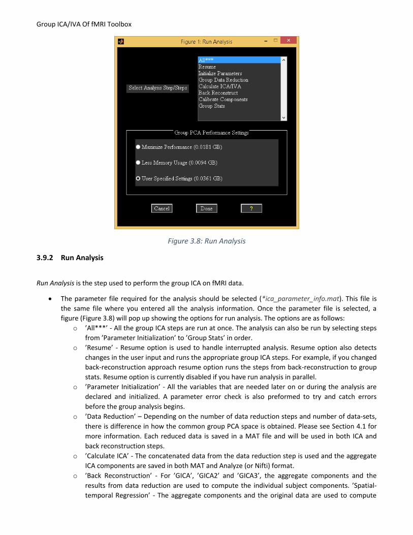
Figure 3.8: Run Analysis
3.9.2 Run Analysis
Run Analysis is the step used to perform the group ICA on fMRI data.
The parameter file required for the analysis should be selected (*ica_parameter_info.mat). This file is
the same file where you entered all the analysis information. Once the parameter file is selected, a
figure (Figure 3.8) will pop up showing the options for run analysis. The options are as follows:
o ’All***’ - All the group ICA steps are run at once. The analysis can also be run by selecting steps
from ’Parameter Initialization’ to ’Group Stats’ in order.
o ’Resume’ - Resume option is used to handle interrupted analysis. Resume option also detects
changes in the user input and runs the appropriate group ICA steps. For example, if you changed
back-reconstruction approach resume option runs the steps from back-reconstruction to group
stats. Resume option is currently disabled if you have run analysis in parallel.
o ’Parameter Initialization’ - All the variables that are needed later on or during the analysis are
declared and initialized. A parameter error check is also preformed to try and catch errors
before the group analysis begins.
o ’Data Reduction’ – Depending on the number of data reduction steps and number of data-sets,
there is difference in how the common group PCA space is obtained. Please see Section 4.1 for
more information. Each reduced data is saved in a MAT file and will be used in both ICA and
back reconstruction steps.
o ’Calculate ICA’ - The concatenated data from the data reduction step is used and the aggregate
ICA components are saved in both MAT and Analyze (or Nifti) format.
o ’Back Reconstruction’ - For ’GICA’, ’GICA2’ and ’GICA3’, the aggregate components and the
results from data reduction are used to compute the individual subject components. ’Spatial-
temporal Regression’ - The aggregate components and the original data are used to compute

Group ICA/IVA Of fMRI Toolbox
the individual subject components. The individual subject components are saved in Analyze (or
Nifti) format.
o ’Calibrating Components’ - By default, components are in arbitrary units. Components are
scaled to percent signal change, Z-scores, scaling in timecourses or scaling in maps and
timecourses.
o ’Group Stats’ - The individual back reconstructed components are used to compute a mean
spatial map and time course, a standard deviation spatial map and time course and a t-statistic
spatial map. The time course used for the t-statistic component is the mean time course. These
group stats components are calculated for each session and are saved in Analyze (or Nifti)
format. Results during each of the steps are printed to the MATLAB command window. After
the analysis is completed, Display GUI (Figure 3.10) will open automatically for visualizing
components.
Group PCA Performance Settings - There are three options like ’Maximize Performance’, ’Less Memory
Usage’ and ’User Specified Settings’. Best match for each option is selected based on the variable
MAX_AVAILABLE_RAM.
o ’Maximize Performance’ - Reduced data-sets from the first data reduction step are stacked by
default.
o ’Less Memory Usage’ – Small groups of data-sets are loaded at a time in a memory.
o ’User Specified Settings’ - User specified PCA options are selected.
Note:
• All the analysis information is stored in the _results.log file. This file gets appended each time the analysis
is run with the same prefix for the output files.
• Run analysis steps can also be accessed from the command line.
load(param_file); % Load parameter file (*ica*param*mat)
sesInfo = icatb_runAnalysis(sesInfo, 1); % Run All Steps
sesInfo = icatb_runAnalysis(sesInfo, 2); % Parameter Initialization
sesInfo = icatb_runAnalysis(sesInfo, 3); % Data Reduction
sesInfo = icatb_runAnalysis(sesInfo, 4); % ICA
sesInfo = icatb_runAnalysis(sesInfo, 5); % Back reconstruction
sesInfo = icatb_runAnalysis(sesInfo, 6); % Scaling components
sesInfo = icatb_runAnalysis(sesInfo, 7); % Group Stats
sesInfo = icatb_runAnalysis(sesInfo, 8); % Resume interrupted analysis
• Option is provided in the GIFT to run a particular data reduction step. This is useful when a particular data
reduction step was already done and you would like to go to the next step without re-running the earlier
step.
load(param_file); % Load parameter file (*ica*param*mat)
sesInfo.reductionStepsToRun = 2; %Run 2nd reduction only
sesInfo = icatb_runAnalysis(sesInfo, 3); % Call Data Reduction
Group ICA/IVA Of fMRI Toolbox
• You could also switch between PCA types using command line. For example, the first data reduction could
be done using standard PCA and the memory intensive second data reduction could be done using
MPOWIT algorithm.
load(param_file); % Load parameter file (*ica*param*mat)
%% Run 1st data reduction using Standard PCA
sesInfo.pcaType = ’standard’; % Standard PCA
sesInfo.reductionStepsToRun = 1; % First reduction
sesInfo = icatb_runAnalysis(sesInfo, 3); % Call data reduction
%% Run 2nd data reduction using MPOWIT
sesInfo.pcaType = ’mpowit’; % MPOWIT
sesInfo.reductionStepsToRun = 2; % Second reduction
sesInfo=icatb_runAnalysis(sesInfo, 3); % Call data reduction
• By default, the component spatial maps and time courses will be written as Nifti files. You have the option
to compress image files according to their viewing set name like subject 1 session 1, mean for session 1,
etc. The variable used for compressing files is ZIP_IMAGE_FILES (Appendix 6.2).
3.9.3 Analysis Info
Analysis Info contains the information about the parameters, data reduction and the output files. Once the analysis is done, click on the Analysis Info button on the GIFT main window and select the parameter file that
you want to look at. Then a figure (Figure 3.9) will pop up showing the information contained within this window.

Group ICA/IVA Of fMRI Toolbox
Figure 3.9: Analysis Info
Figure 3.10: Display GUI

Group ICA/IVA Of fMRI Toolbox
3.10 VISUALIZATION METHODS
3.10.1 Display GUI
GIFT contains three main ways of visualizing the components after analysis like the Component Explorer, the
Composite Viewer and the Orthogonal Viewer. These three visualization options can be used independently
(Display Tools in Figure 3.2) or collectively using the Display GUI. This visualization tool provides the user an easy
way to explore all the three visualization options along with subject component explorer.
The selected visualization method will be highlighted in colored text. By default, Component Explorer
visualization method will be selected after selecting the parameter file. Figure 3.10 shows the main user
interface controls. Some of the user-interface controls are shielded from the user and plotted in the ”Display
Defaults” menu (Figure 3.11). All the display parameters are explained below followed by explanation of
visualization methods:
Main user interface controls
• ’Sort Components’ - Components will be sorted spatially or temporally. This control will be enabled only
for Component Explorer visualization methods.
• ‘Viewing Set’ - This is the component viewing set to look at like subject 1 session 1, mean for session 1, etc
and will be disabled for Subject Explorer visualization method.
• ’Component number’ - Component number/numbers to look at. This will be disabled for Component
Explorer visualization method.
• Load Anatomical - Load Anatomical button is used to select anatomical image. Component images will be
overlaid on this anatomical image. By default, first image of functional data will be used as an anatomical
image.
• Display - Display button is used to display the components of different visualization methods.
• Display Defaults menu - Hidden display parameters will be shown in a figure (Figure 3.11) when you click
on Display Defaults menu. This figure contains parameters like ’Image Values’, ’Anatomical Plane’,
’Threshold’, ’Slice Range’ and ’Images Per Figure’. ”Display GUI Options” menu can be used to change
design matrix and selecting the text file (See Appendix 6.2) that contains regressor information for
temporal sorting. Select ’Design Matrix’ for selecting design matrix for temporal sorting. There are three
options for selecting design matrix like ’Same regressors for all subjects and sessions’, ’Different regressors
over sessions’, ’Different regressors for subjects and sessions’. The options are explained below:
– ’Same regressors for all subjects and sessions’ - The regressors used will be the same over data-sets.
This will open a figure window for selecting SPM design matrix.
– ’Different regressors over sessions’ - The regressors used will be the same over subjects but different
over sessions. This will open a figure window for selecting SPM design matrix.

Group ICA/IVA Of fMRI Toolbox
– ’Different regressors over subjects and sessions’ - Different regressors can be used for each subject’s
session. This will open a figure window for selecting a design matrix for each subject.
User Controls in Display Defaults menu
• ’Image Values’ - There are four options like ’Positive’, ’Positive and Negative’, ’Absolute’, ’Negative’.
’Positive’ and ’Negative’ refer to activations and de-activations on spatial map. You should also look at the
time course (flipped or un-flipped) to make the conclusion.
• ’Convert To Z-scores’ - Converts spatial maps to z-scores.
• ’Threshold Value’ - This is the Z threshold value.
• ’Images Per Figure’ - Number of images per figure for Component Explorer and Subject Explorer
visualization methods.
• ’Anatomical Plane’ - This is the anatomical plane to look at for Component Explorer, Subject Explorer and
Composite Viewer.
• ’Slices Range’ - Slices plotted in mm. Slices in mm are calculated based on the anatomical data. You can
change this setting to not use the slices based on the anatomical data by setting
USE_DEFAULT_SLICE_RANGE variable value to 1 and specify the slices you want to plot in variable
SLICE_RANGE.
Figure 3.11: Display defaults

Group ICA/IVA Of fMRI Toolbox
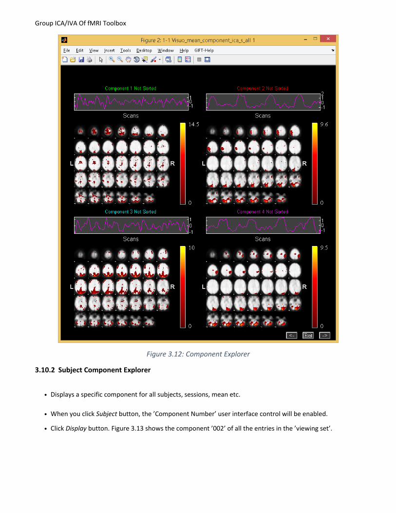
3.10.1.1 Component Explorer
• Component Explorer is used to display all components of a particular viewing set. Therefore, ’Component
Number’ control (Figure 3.10) will be disabled for this visualization method.
• Figure 3.10 shows the selected parameters for the Component Explorer. Click on Display button and wait
for the figures containing spatial maps to pop up. Figure 3.12 shows all the components of mean for all
subjects and sessions in groupings of four. By default all the slices in axial plane are plotted. You can
change these parameters by clicking on menu ”Display Defaults” (Figure 3.11).
• The time course for each component is displayed on the top of the figure (Figure 3.12). The color bar for
each component is displayed next to it. Click on the time course for an enlarged view. Look through the
components by clicking on the arrow keys at the bottom of each figure. Find the components of interest
and take a note. With this data-set you should find two task related components and one transiently
related component. The task related components show activation in the visual cortex. The act of classifying
components becomes more difficult with more complex tasks and is the motivation for adding the sorting
option.
Group ICA/IVA Of fMRI Toolbox
Figure 3.12: Component Explorer
3.10.2 Subject Component Explorer
• Displays a specific component for all subjects, sessions, mean etc.
• When you click Subject button, the ’Component Number’ user interface control will be enabled.
• Click Display button. Figure 3.13 shows the component ’002’ of all the entries in the ’viewing set’.

Group ICA/IVA Of fMRI Toolbox
Figure 3.13: Subject Component Explorer

Group ICA/IVA Of fMRI Toolbox
3.10.3 Orthogonal Explorer
• Orthogonal viewer is used to look at a component and compare it to the functional data.
• Figure 3.14 shows one of the task related components.
• Upper plot is the BOLD time course for the selected data-set in the popup window at the current voxel.
You can interactively select voxel by clicking on any of the slices. Lower plot shows the ICA time course for
the maximum voxel (red), minimum voxel (dotted red) and the selected voxel (green).
• When you click on Plot button top five components (of the selected viewing set in Display GUI) for the
selected voxel will be displayed. The maximum voxel and the location will be printed to the command
prompt. Option (Click on ”Options” menu) is provided in the Figure 3.14 to enter the voxel (real world
coordinates) instead of navigating around the brain.
Figure 3.14: Orthogonal Explorer
3.10.4 Composite Viewer

Group ICA/IVA Of fMRI Toolbox
Composite viewer is used to look at multiple components of interest. Use the component explorer to find the
task related components. In the ’Component Number’ user interface control, select the two components that
are task related. At most five different components can be overlaid on one another. We used anatomical image
ch2bet.nii from folder icatb/icatb_templates. Slices -40:4:72 mm are selected (Figure 3.11). When you click
Display button, Figure 3.15 will open in a new window.
Figure 3.15: Composite Viewer

Group ICA/IVA Of fMRI Toolbox
Figure 3.16: Selected parameters for sorting the components temporally.
3.11 SORTING COMPONENTS
Sorting is a way to classify the components. The components can be sorted either spatially or temporally. For
every independent component spatial maps and time courses are generated. Temporal sorting is a way to
compare the model’s time course with the ICA time course whereas spatial sorting classifies the components by
comparing the component’s image with the template. When you click Component button, ’Sort Components’
popup box will be enabled. Select ’Yes’ for ’Sort Components’. Click Display button then a figure (Figure 3.16)
will open in a new window. We have implemented three different types of sorting criteria like Correlation,
Kurtosis and Multiple Linear Regression (MLR). MLR can be a very useful method in separating the two task
related components. First, temporal sorting is explained followed by spatial sorting. The following are the steps
involved in sorting components:
3.11.1 Temporal Sorting
Multiple regression sorting criteria is used to explain the temporal sorting. We select all data-sets (concatenated
ICA time courses) and correlate with model time course. The regressors selected are ”right*bf(1)”, ”right*bf(2)”,
”left*bf(1)” and ”left*bf(2)” time courses. After the calculation is done, components are sorted based on the R-
square statistic. The R-square statistic values and the slopes of the regressors are printed to a text file with the
suffix regression.txt. Partial correlations and the slopes of the regressors are printed to a text file with the suffix
partial_corr.txt. Figure 3.17 shows the components sorted based on the MLR sorting criteria in groupings of
four. Here you can see that the first two components are task related. For a larger view of the time course plot
(Figure 3.18) click on the time course plot in the main window. A list of menus is plotted on the time course plot.
The explanation of each menu will be explained below:

Group ICA/IVA Of fMRI Toolbox
Utilities: Utilities contain sub menus like ”Power Spectrum”, ”Split-time courses” and ”Event Average”.
When you click ”Split-time courses” sub menu, split of the time courses (Figure 3.19) will be shown. Click
on sub menu ”Event Average” and select ”right*bf(1)” reference function to plot the event averages ()
of the ICA time courses. Explanation of the event average is given in Section 3.12.10.
Options: ”Options” menu has sub menus like ”Timecourse Options”, and ”Adjust ICA”.
o Timecourse Options: When you click on sub menu ”Timecourse Options”, a new figure window
will open that has options for detrending the ICA time course, model time course and options
for event average. Explanation of this figure window is given in the Appendix 6.3. Leave the
defaults as shown in the figure.
o Adjust ICA: Option is provided in this sub-menu to remove the variance of other than selected
regressor. When you click on sub menu ”Adjust ICA”, a list dialog box will open to select the
reference function. For now select the ”right*bf(1)” time course. The ICA time course is adjusted
by removing the line fit of the model with the ICA time course where model contains nuisance
parameters and other than the selected reference function. After the ICA time course is
adjusted the plot is shown in the expanded view time course plot (Figure 3.21). When you click
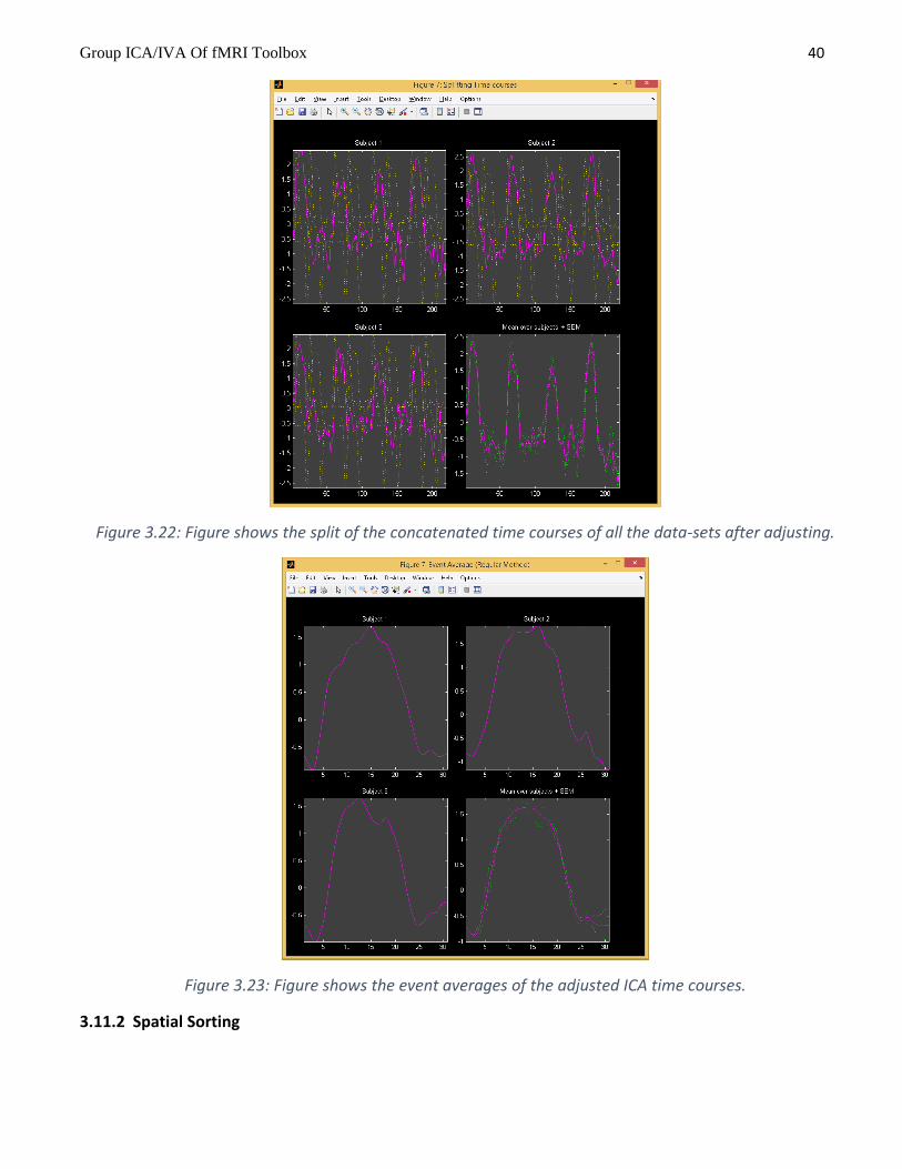
on the sub menu ”Split-time courses” in ”Utilities” menu, a new figure window (Figure 3.22)
showing the split of the adjusted ICA time courses will be shown. Similarly click on sub menu
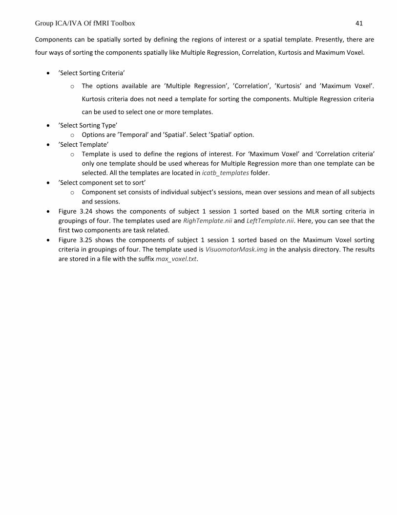
”Event-Average” in ”Utilities” menu and select the ”right*bf(1)” reference function to view the
event averages (Figure 3.23) of the new ICA time courses.
Note: Event average can also be done without sorting components (Section 3.12.10). Please see Appendix 6.2
for entering regressors through a text file for large data-sets.

Group ICA/IVA Of fMRI Toolbox
Figure 3.17: Components are sorted based on Multiple Regression criteria in groupings of four.

Group ICA/IVA Of fMRI Toolbox
Figure 3.18: Enlarged view of task related timecourse
Figure 3.19: Figure shows the split of the concatenated time courses of all the data-sets. Mean is calculated over all data-sets

Group ICA/IVA Of fMRI Toolbox 39
Figure 3.20: Event average
Figure 3.21: Enlarged view of task related timecourse after removing variance of other than the selected regressor (“right*bf(1)”).
Group ICA/IVA Of fMRI Toolbox 40
Figure 3.22: Figure shows the split of the concatenated time courses of all the data-sets after adjusting.
Figure 3.23: Figure shows the event averages of the adjusted ICA time courses.
3.11.2 Spatial Sorting
Group ICA/IVA Of fMRI Toolbox 41
Components can be spatially sorted by defining the regions of interest or a spatial template. Presently, there are
four ways of sorting the components spatially like Multiple Regression, Correlation, Kurtosis and Maximum Voxel.
’Select Sorting Criteria’
o The options available are ’Multiple Regression’, ’Correlation’, ’Kurtosis’ and ’Maximum Voxel’.
Kurtosis criteria does not need a template for sorting the components. Multiple Regression criteria
can be used to select one or more templates.
’Select Sorting Type’
o Options are ’Temporal’ and ’Spatial’. Select ’Spatial’ option.
’Select Template’
o Template is used to define the regions of interest. For ‘Maximum Voxel’ and ‘Correlation criteria’
only one template should be used whereas for Multiple Regression more than one template can be
selected. All the templates are located in icatb_templates folder.
’Select component set to sort’
o Component set consists of individual subject’s sessions, mean over sessions and mean of all subjects
and sessions.
Figure 3.24 shows the components of subject 1 session 1 sorted based on the MLR sorting criteria in
groupings of four. The templates used are RighTemplate.nii and LeftTemplate.nii. Here, you can see that the
first two components are task related.
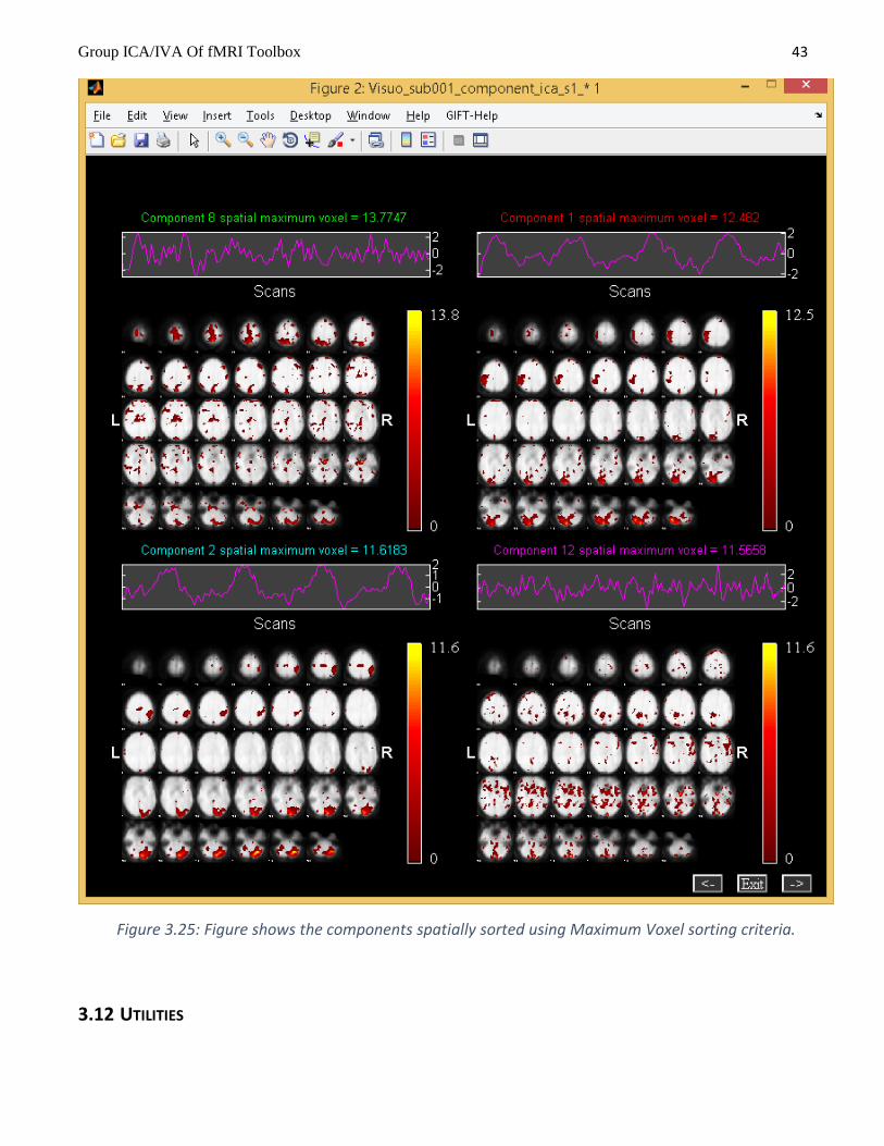
Figure 3.25 shows the components of subject 1 session 1 sorted based on the Maximum Voxel sorting
criteria in groupings of four. The template used is VisuomotorMask.img in the analysis directory. The results
are stored in a file with the suffix max_voxel.txt.

Group ICA/IVA Of fMRI Toolbox 42
Figure 3.24: Figure shows the components spatially sorted using Multiple Regression sorting criteria.
Group ICA/IVA Of fMRI Toolbox 43
Figure 3.25: Figure shows the components spatially sorted using Maximum Voxel sorting criteria.
3.12 UTILITIES

Group ICA/IVA Of fMRI Toolbox 44
3.12.1 Generate Mask
We now provide an option to generate average mask and exclude outlier subjects from the analysis by correlating an
average mask with the individual masks. To invoke the tool, use “Generate mask” under “Utilities” (See Figure 3.2)
drop down box. The following figure window will open after you have selected output directory:
Figure 3.26: Data selection
Select data for all the subjects. If data is in 3D analyze image format, enter the full file pattern using ED button. Input
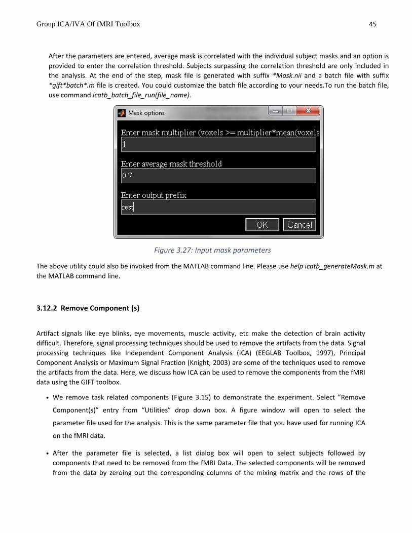
screen window (Figure 3.27) will open to enter mask specific defaults:
Enter mask multiplier: Voxels above or equaling the multiplier times the mean is included for each subject.
Only the first volume is used in the mask calculation for each subject.
Enter average mask threshold: Binary masks are averaged across subjects and threshold is applied on the
average mask.
Enter output prefix: All the output files will have this prefix.
Group ICA/IVA Of fMRI Toolbox 45
After the parameters are entered, average mask is correlated with the individual subject masks and an option is
provided to enter the correlation threshold. Subjects surpassing the correlation threshold are only included in
the analysis. At the end of the step, mask file is generated with suffix *Mask.nii and a batch file with suffix
*gift*batch*.m file is created. You could customize the batch file according to your needs.To run the batch file,
use command icatb_batch_file_run(file_name).
Figure 3.27: Input mask parameters
The above utility could also be invoked from the MATLAB command line. Please use help icatb_generateMask.m at
the MATLAB command line.
3.12.2 Remove Component (s)
Artifact signals like eye blinks, eye movements, muscle activity, etc make the detection of brain activity
difficult. Therefore, signal processing techniques should be used to remove the artifacts from the data. Signal
processing techniques like Independent Component Analysis (ICA) (EEGLAB Toolbox, 1997), Principal
Component Analysis or Maximum Signal Fraction (Knight, 2003) are some of the techniques used to remove
the artifacts from the data. Here, we discuss how ICA can be used to remove the components from the fMRI
data using the GIFT toolbox.
• We remove task related components (Figure 3.15) to demonstrate the experiment. Select ”Remove
Component(s)” entry from “Utilities” drop down box. A figure window will open to select the
parameter file used for the analysis. This is the same parameter file that you have used for running ICA
on the fMRI data.
• After the parameter file is selected, a list dialog box will open to select subjects followed by
components that need to be removed from the fMRI Data. The selected components will be removed
from the data by zeroing out the corresponding columns of the mixing matrix and the rows of the
Group ICA/IVA Of fMRI Toolbox 46
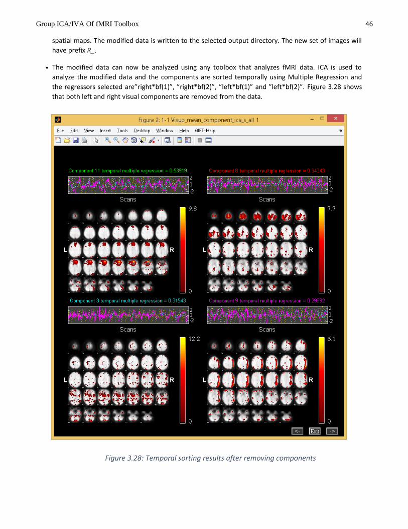
spatial maps. The modified data is written to the selected output directory. The new set of images will
have prefix R_.
• The modified data can now be analyzed using any toolbox that analyzes fMRI data. ICA is used to
analyze the modified data and the components are sorted temporally using Multiple Regression and
the regressors selected are”right*bf(1)”, ”right*bf(2)”, ”left*bf(1)” and ”left*bf(2)”. Figure 3.28 shows
that both left and right visual components are removed from the data.
Figure 3.28: Temporal sorting results after removing components

Group ICA/IVA Of fMRI Toolbox 47
Figure 3.29: Stats on beta weights GUI
Figure 3.30: Group selection
3.12.3 Temporal Sorting

Group ICA/IVA Of fMRI Toolbox 48
We now provide a stand-alone option for doing temporal sorting using all data-sets and selected regressors of
interest. This option is useful if you have cross-task SPM design matrices which have different regressor names or
missing conditions across some subjects. Multiple regression is computed using the ICA timecourses as observations
and timecourses in SPM design matrix as model. One sample t-test is computed on the beta weights for each run
and condition and saved in “temporal_stats” field in the ICA parameter file. An option is provided to export results
to PDF or HTML file formats. Figure 3.31 shows T-values of each run and condition for a component. This utility could
also be invoked using function “icatb_temp_regress.m”.
Figure 3.31: One sample t-test on beta weights
3.12.4 Stats On Beta Weights
This utility is provided to test the significance of the component time courses by doing statistics on the beta
weights, which are obtained after doing temporal sorting on all data-sets. Design criteria like one sample t-
test, two sample t-test, one way anova (groups), one way anova (regressors), two way anova (groups,
regressors) and Multiple Regression are provided. The following are the steps involved:
When you select ”Stats On Beta Weights” option in ”Utilities” drop down box (Figure 3.2), a figure
window will open to select the regression parameters text file, which is obtained during temporal
sorting of all data-sets.
After selecting regression parameters text file, an option is provided to average beta weights across
runs or sessions. Figure 3.29 shows the GUI for doing stats on beta weights.
The parameters in the figure are explained below:
o ”Select design criteria” - Options provided are ’one sample t-test’, ’two sample t-test’, ’one
way anova (groups)’, ’one way anova (regressors)’, ’two way anova (groups, regressors)’ and
’Multiple Regression’.
o Groups Listbox - You can add groups using + button adjacent to groups listbox. Figure 3.30
will open to select subjects and sessions for that group. You can also use edit box below the
listbox to select the subjects, if the subject numbers are stored in ascii file by entering
load(’c:\sub1.asc’) or using any other valid MATLAB expression. Each group added will be an

Group ICA/IVA Of fMRI Toolbox 49
entry in groups listbox. You need to double click on the entry or press enter key to view or
make any changes to the selected group. To remove the selected groups use - button
adjacent to groups listbox.
o Regressors Listbox - You can select only one regressor for one sample t-test and two sample
t-test whereas for Anova and Multiple Regression you can select multiple regressors.
o Contrasts Listbox - This option is provided to do Anova contrasts. To add a contrast use +
button adjacent to contrasts listbox. Sum of contrast vector must equal to zero. The length
of contrast vector to enter will change depending on the design criteria. The description is as
follows:
One way anova (Groups) - Length of contrast vector is equal to the number of
selected groups. For example if there are 2 groups contrast vector must be of length
2.
One way anova (Regressors) - Length of contrast vector is equal to the number of
selected regressors. For example if there are 4 regressors contrast vector must be of
length 4.
Two way anova (Groups, Regressors) - Length of contrast vector is equal to the
number of selected groups and regressors. For example if there are 2 groups and 4
regressors, contrast vector must be of length 6. First 2 entries correspond to groups
and the next 4 entries correspond to regressors.
Note: You need to use double click or press enter key on the selected contrast, if you decide to
change the name of the contrast or value of the contrast vector.
Calculate - Statistics are done after selecting the design criteria, groups, regressors and contrasts
(Figure 3.29). All the results are printed to a file with suffix summary.txt. This file also contains mean
and standard deviation for each condition of a group. An additional option is provided for one way
anova (groups) to do operation on regressors and treat it as a single regressor. For example, if you
have selected two regressors like targets and novels to test the significance of components. You can
directly subtract targets and novels and do a one way anova (groups) by specifying [1 -1] for the
equation of regressors.
Note:
When you select Multiple regression tool, a figure window will open to select the regressor file or
files like age, test scores, etc. After you selected the regressor files, R-square statistic is calculated for
each component. We also report the slopes and partial correlations of the regressors.
Option is provided to do statistics on the beta weights using a batch file. Please see Section 3.14.3
for more information.
If you wish to use your favorite statistics package to do the statistics on the beta weights,
icatb_parse_regression_mat function is provided that will write regression parameters in a excel file
or load it in the MATLAB command window. Type help icatb_parse_regression_mat.m for more
information.

Group ICA/IVA Of fMRI Toolbox 50
3.12.5 SPM Stats
You can test the significance of components by doing a one sample t-test or two sample t-test on subject component images. We provide options to do one sample, two sample and paired t-tests using SPM (SPM5/SPM8/SPM12).
One sample t-test - One sample t-test for each component will be automatically calculated if you set variable SPM_STATS_WRITE_TAL in icatb_defaults.m to 1 or 2. If you set variable SPM_STATS_WRITE_TAL value to 1 only one sample t-test will be calculated whereas a value of 2 will also write talairach tables for the t-map.
o Note: An option is also provided in ”Utilities” (Figure 3.2) drop down box to calculate t-maps for the selected data-sets.
Two sample t-test - When you click ”Utilities” (Figure 3.2) drop down box and have selected ”SPM Stats” as the option, a figure window will open to select the design criteria. When you select design as ”Two sample t-test”, two sample t-test for a component will be calculated between the selected groups by using an explicit mask. The explicit mask is calculated by applying a threshold (SPM_STATS_TTEST_THRESHOLD) on t-map obtained by doing a one sample t-test on data-sets.
o Note: When you set SPM_STATS_TTEST2_EXPLICIT_MASK variable in icatb_defaults.m file to 0, explicit mask is not used.
3.12.6 Spatial-temporal Regression
GLM or ICA spatial maps are used as design matrix and the original data of subjects as observations to reconstruct individual subject components using Multiple Regression. This utility can also be invoked from the MATLAB command line. compFiles={'E:\Multiple_sub_Multiple_sess\sens\Sensorimotor_agg__component_ica_018.img',... 'E:\Multiple_sub_Multiple_sess\sens\Sensorimotor_agg__component_ica_019.img'}; inputFiles={'F:\smr1\swSm_nifti.nii', 'F:\smr2\swSm_nifti.nii'}; icatb_spatial_temp_regress(compFiles, inputFiles, 'outputDir', '.','format', '.nii', 'outputPrefix', 'STR'); Where compFiles and inputFiles must be in a cell array. Each cell in inputFiles can contain a character array of 3D analyze images. The resulting subject components are saved in the specified format and the selected output directory. These components can be displayed in GIFT by using display tools like Component Explore, Orthogonal Viewer and Composite Viewer (Figure 3.2).
3.12.7 Write Taliarach Table We use Talairach Daemon software for generating talairach tables. When you select ”Write Talairach Table”
option in ”Utilities” (Figure 3.2) drop down box, a figure window will open to select the image. We apply a
threshold from variable TALAIRACH_THRESHOLD and write talairach coordinates for positive and negative
regions in separate excel files.
3.12.8 Component Labeler
Option is provided to label components given the templates of interest. We provide templates in
icatb/icatb_templates/RSN.zip file and description about the templates in icatb/icatb_templates/RSN.txt. Each

Group ICA/IVA Of fMRI Toolbox 51
component is correlated with the given templates and best template is selected based on the maximum correlation
value. Figures below shows the component labeler GUI and one of the labeled components.
Figure 3.32: Component Labeler GUI
Figure 3.33: One of the labeled components. Also correlation value w.r.t template is displayed.
3.12.9 Ascii To SPM.mat
Group ICA/IVA Of fMRI Toolbox 52
Temporal sorting is done using a SPM design matrix. You can create SPM design matrix from a ascii file
containing regressor time courses using ”Utilities” (Figure 3.2) drop down box. Under ”Utilities” drop down
box select Ascii_to_spm.mat. The time course matrix is of dimensions m by n where m is the sum of the
number of scans over sessions and n is the number of total regressors. Type help icatb_formDesignMat at
the MATLAB command prompt for an example. See icatb_templates folder for example regressor data files.
3.12.10 Event Average
Event related average means the average of the events in the ICA time course. Events are calculated based
on the onsets of the selected reference function or model time course. GIFT also provides the user to
calculate the event average without sorting the components temporally. Under ”Utilities” drop down box
(Figure 3.2) select ”Event Average”. This will open a figure window to select the parameter file. After
selecting the parameter file you can specify the subjects, sessions, component and reference function
required for event average.
Note:
• For large data-sets regressors can be entered through a sorting text file (Appendix 6.2). The first regressor
specified in the text file will be used for event average.
• ICA time courses are not adjusted when calculating event average using ”Utilities” drop down box in . Please
see Section 3.11.1 for calculating event average with the variance removal (”Adjust ICA”) tool.
3.12.11 Calculate Stats
Option is provided under ”Utilities” drop down box (Figure 3.2) to calculate the statistics for the required
data-sets over sessions or subjects or subjects and sessions. The resulting set of images can be used in SPM
to do multi-group comparisons (between subjects or sessions) like two sample t-test.
Note: The images created using ”Calculate Stats” under ”Utilities” drop down box cannot be viewed using
Display GUI and therefore, display tools like Component Explorer, Composite Viewer and Orthogonal Viewer
in must be used (Figure 3.2).
3.12.12 Spectral Group Compare
Group comparison of time courses is done by comparing the power spectra between the groups at different
frequency bins. The results of the power spectra comparison is saved in a MAT file having suffix
*comparison_frequency_bins.mat. The variables stored in the file are as follows:
mean_power_group1 - Mean power for group 1.
mean_power_group2 - Mean power for group 2.
tValues - T-values. This variable is used for plotting the bar graphs.
pValues - p-values.

Group ICA/IVA Of fMRI Toolbox 53
fftPlots – Power spectra for all subjects of dimensions subjects by components by spectral length.
Figure 3.34 shows the T-values of the components in groupings of four at different frequency bins. Bins are labeled
using the variable DEFAULT_TR_SPECTRAL_GROUP_COMPARE.
Figure 3.34: Spectral group comparison between groups
3.12.13 Single Trial Amplitudes
Single trial amplitudes are the beta weights which are obtained by doing a Multiple Regression of the design matrix and the ICA time course where the design matrix is obtained by doing a convolution of the onsets and the event averages. This utility must be used after doing temporal sorting of all data-sets in the GIFT and using only the regressors of interest. The best regressor onsets for each data set are used to compute single trial amplitudes and event averages. We determine the best regressor for each data-set based on the maximum beta weight value (not the absolute value). Figure 3.35 shows the orthogonal slices at the maximum voxel, event average and the single trial amplitudes for the selected components. We also store the single trial amplitude results in a file having suffix *single_trial_results.mat.

Group ICA/IVA Of fMRI Toolbox 54
Figure 3.35: Single Trial Amplitudes
3.12.14 Z-shift
Z-shift is used to center the image distribution to zero based on the peak of the distribution. Please select the
file or files of interest. The function used for computing Z-shift is icatb_convert_to_z_shift. This tool is
redundant as the back-reconstructed component images are already centered by default in GIFT (Please see
CENTER_IMAGES variable in icatb_defaults.m).
3.12.15 Percent Variance
Percent variance utility can be used after running a group ICA analysis. Percent variance explained by the components in the data is calculated by doing a Multiple Regression of the BOLD signal and the component time

Group ICA/IVA Of fMRI Toolbox 55
courses at each voxel where the component time courses are treated as a model. After the calculation is done, the final result is printed to the MATLAB command window.
3.13 TOOLBOXES
3.13.1 ICASSO
ICASSO toolbox (ICASSO Toolbox, 2003) is used in GIFT to determine the reliability of ICA algorithm. ICA
algorithm is run several times to determine the algorithmic reliability or stability. Reliable estimates
correspond to tight clusters and unreliable ones do not point to any cluster. Figure 3.36 will open when you
select “ICASSO” under ”Toolboxes” drop down box (Figure 3.2). The parameters in the Figure 3.36 are as
follows:
”Select Mode” - Options available are ’RandInit’, ’Bootstrap’ and ’both’. The explanation of each
option is given below:
o ’RandInit’ - Algorithm starts with different initial values.
o ’Bootstrap’ - Bootstrap technique is used.
o ’both’ - Uses both ’RandInit’ and ’Bootstrap’ options.
”Select number of ICA runs” - Number of times ICA algorithm will be run.
“Enter min cluster size” - Enter minimum cluster size. It is preferred to use a value of 0.8 times the
number of ICA runs.
“Enter min cluster size” - Enter maximum cluster size. It is preferred to use a value equal to the
number of ICA runs.
We ran ICA 10 times on Infomax algorithm and extracted 16 components from the data. Figure 3.37 shows
the results of Infomax algorithm. ICASSO results are written to a MAT file with suffix _icasso_results.mat.
This MAT file contains the following variables:
iq - Stability index.
sR - Variable containing information about similarity measure, clustering and projection.
A - Mixing matrix.
W - Un-mixing matrix.
S - Source signal.
Since ICASSO uses clustering of components and there is no constraint in ICASSO on the number of components within each cluster. A cluster containing more components than runs might combine components from different functional areas. Also the mixing coefficients of centrotype might come from different runs which might not be desirable as well. To avoid this stable run estimates are used. These estimates are calculated using stability index,
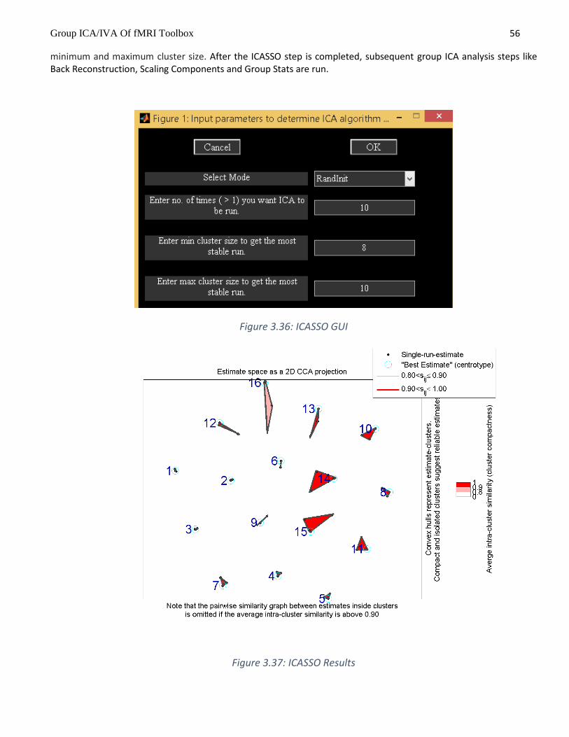
Group ICA/IVA Of fMRI Toolbox 56
minimum and maximum cluster size. After the ICASSO step is completed, subsequent group ICA analysis steps like Back Reconstruction, Scaling Components and Group Stats are run.
Figure 3.36: ICASSO GUI
Figure 3.37: ICASSO Results

Group ICA/IVA Of fMRI Toolbox 57
3.13.2 Mancovan
Mancovan toolbox is based on the paper (E. Allen, E. Erhardt, E. Damaraju, W. Gruner, J. Segall, R. Silva, M.
Havlicek, S. Rachakonda, J. Fries, R.Kalyanam, A. Michael, J. Turner, T. Eichele, S. Adelsheim, A. Bryan, J. R.
Bustillo, V. P. Clark, S. Feldstein,F. M. Filbey, C. Ford, et al, 2011). This toolbox works on MATLAB versions
greater than R2008a. Features used are subject component spatial maps, timecourses spectra and FNC
correlations. Multivariate tests are done on the features to determine the significant covariates which are
later used in the univariate tests on each feature. To invoke the toolbox, select “Mancovan” under
“Toolboxes” menu (Figure 3.2). You could also invoke toolbox using mancovan_toolbox at the command
prompt. Mancovan toolbox (Figure 3.38) is divided into four parts like create design matrix, setup features,
run mancova and display. Each step is explained below:
Figure 3.38: Mancovan Toolbox
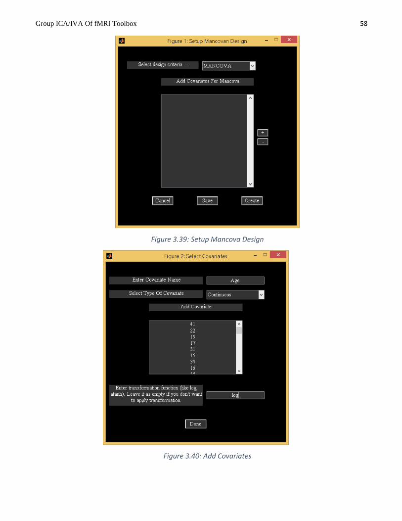
Group ICA/IVA Of fMRI Toolbox 58
Figure 3.39: Setup Mancova Design
Figure 3.40: Add Covariates

Group ICA/IVA Of fMRI Toolbox 59
Create design matrix
When you click on Create Design Matrix button, a figure window will open to select the ICA parameter file.
All the output files will have prefix prefix_mancovan where prefix is from ICA parameter file. Figure 3.39
shows the initial mancovan setup screen. Options for “Select design criteria” are “Mancova”, “One sample t-
test”, “Two sample t-test” and “Paired t-test”.
Mancova - Add covariates of interest using + button next to the listbox (Figure 3.39). You could type
covariate values by hand or use right click on the edit box (Figure 3.40) and this will open a figure
window to load the ascii file for continuous covariates. For categorical covariates, specify labels to
distinguish the levels. Each covariate vector must have length equal to no. of subjects in the original
ICA analysis. Option is also provided to apply transformation function to the continuous covariates.
Use create button to create the design matrix. Design information is stored in mancovan parameter
file *mancovan.mat. At the end, option is provided to select subjects to model time. Currently, at
most paired samples are handled. Modeling time covariate involves computing mancova for each
timepoint and mancova on difference between the timepoints.
The following options does univariate tests on features automatically bypassing the multivariate
step:
o One sample t-test – Components are averaged across sessions. Select subjects for doing one
sample t-test.
o Two sample t-test - Components are averaged across sessions. Select subjects for group 1
and group for doing two sample t-test between groups.
o Paired t-test - Option is provided to select data-sets for condition 1 and condition 2.
Setup Features
When you click on Setup Features button (Figure 3.38), a figure window will open to select the mancovan
parameter file. The following are the steps involved:
Features - Select feature or features of interest (Figure 3.41).
Add ICA components - Enter component networks using + button.
p-value significance - Enter p-value significance threshold which will be used in multivariate and
univariate tests.
Enter TR in seconds - Enter TR of the original data in seconds. This information will be used in computing
spectra and filtering of timecourses.
Enter no. of principal components - Enter no. of principal components for each feature in a vector. The
entered components should not exceed the minimum feature dimensions. Maximum number of
principal components you could select for each feature is dependent on the actual degrees of freedom
in the data. Approximate degrees of freedom for each feature is as shown below:
o Spatial maps – Minimum of voxels and subjects.
o Spectra – Minimum of spectral length and subjects.
o FNC correlations – Minimum of number of ICA component pairs and subjects.
Mancovan defaults - Mancovan defaults (Figure 3.42) will open when you use ”Mancovan defaults”
menu. The defaults for each feature are as follows:
o Spatial Maps - You could use the user specified mask or default mask. Default mask includes the
voxels based on the distribution of voxelwise t-statistics. Only the voxels with strong and
consistent activation across subjects are included.
o Timecourses Spectra - The following are the options:
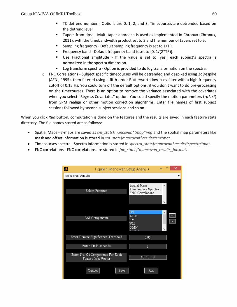
Group ICA/IVA Of fMRI Toolbox 60
TC detrend number - Options are 0, 1, 2, and 3. Timecourses are detrended based on
the detrend level.
Tapers from dpss - Multi-taper approach is used as implemented in Chronux (Chronux,
2011), with the timebandwidth product set to 3 and the number of tapers set to 5.
Sampling frequency - Default sampling frequency is set to 1/TR.
Frequency band - Default frequency band is set to [0, 1/(2*TR)].
Use Fractional amplitude - If the value is set to ’yes’, each subject’s spectra is
normalized in the spectra dimension.
Log transform spectra - Option is provided to do log transformation on the spectra.
o FNC Correlations - Subject specific timecourses will be detrended and despiked using 3dDespike
(AFNI, 1995), then filtered using a fifth-order Butterworth low-pass filter with a high frequency
cutoff of 0.15 Hz. You could turn off the default options, if you don’t want to do pre-processing
on the timecourses. There is an option to remove the variance associated with the covariates
when you select “Regress Covariates” option. You could specify the motion parameters (rp*txt)
from SPM realign or other motion correction algorithms. Enter file names of first subject
sessions followed by second subject sessions and so on.
When you click Run button, computation is done on the features and the results are saved in each feature stats
directory. The file names stored are as follows:
Spatial Maps - T-maps are saved as sm_stats\mancovan*tmap*img and the spatial map parameters like
mask and offset information is stored in sm_stats\mancovan*results*sm*mat.
Timecourses spectra - Spectra information is stored in spectra_stats\mancovan*results*spectra*mat.
FNC correlations - FNC correlations are stored in fnc_stats\*mancovan_results_fnc.mat.

Group ICA/IVA Of fMRI Toolbox 61
Figure 3.41: Setup Features
Figure 3.42: Mancova Setup Defaults
Run Mancovan
Select the mancovan parameter file which was created after the end of setup features step. A figure window will open to select nuisance covariates to be removed from the features. For example, you could remove site related variance from the features before computing mancova. By default, multivariate tests are computed followed by univariate tests on the covariates which are significant in the multivariate step (Figure 3.43). If you selected option “yes” for question “Do you want to skip multivariate tests?” (Figure 3.43), multivariate tests part is skipped and univariate tests are done only on the selected covariates. All covariates are shown in the listbox on the left hand side. In the middle listbox, you could add covariates of interest and for each selected covariate you could optionally remove variance associated with the other covariates (right listbox). After the selection is done, mancova is done on each feature. Multivariate and univariate test results (‘MULT’ and ‘UNI’) are saved in the *stats\*mancovan*results*mat files.

Group ICA/IVA Of fMRI Toolbox 62
3.43: Run mancovan GUI
Display Mancovan When you click Display button (Figure 3.38), Figure 3.44 will open.
• Features - Features will be displayed when you select features and click on display button. Figure 3.45
and Figure 3.46 show orthogonal views of T-maps, power spectra, and FNC correlations. T-maps are
thresholded using the threshold specified under “threshold” edit box. You can interactively browse
using mouse within each slice. Low frequency and high frequency limits are used to compute fALFF
values.
• Multivariate results - Significant results of covariates will be plotted in a matrix of dimensions
covariates by components (Figure 3.47).
• Univariate results - Univariate results of age covariate are shown for each feature in Figures Figure
3.48-Figure 3.51 . Un-corrected p < 0.05 threshold is used. Description of each plot is shown below:

Group ICA/IVA Of fMRI Toolbox 63
o Spatial maps – In the top row of the plot (Figure 3.48), composite maps of significant effects
over all components are displayed as −sign(t)log10(p). Effects are considered significant if test
statistics exceeded the p < 0.05 threshold with a cluster extent of at least 27 contiguous
voxels. Bottom row of the plot shows average β values over significant clusters with effects of
the same directionality and the color of the bar is proportional to the fraction of component
voxels contributing to each effect.
o Timecourses spectra - In the top row of the plot (Figure 3.51), covariates significance is
shown as a function of frequency for each component displayed as −sign(t)log10(p). Bottom
row of the plot shows β-values averaged over frequency bands with effects of the same
directionality where test statistics exceeded the p < 0.05 threshold. The color of the bar is
proportional to the fraction of contributing frequency bins. The absence of a bar indicates
that univariate tests were not performed or test statistics were not significant.
o FNC Correlations - Significance and direction of each pairwise correlation is displayed as the
−sign(t)log10(p). You have the option to display mean FNC correlations for each level in
categorical covariate when you use right click on each covariate axes provided the covariate
is significant. Figure 3.49 shows the significant univariate results. Also, connectogram of the
FNC univariate results is shown in Figure 3.50. By default, mean components of all data-sets
is used to plot the thumbnails of the spatial maps.
Note: Option is now provided to export mancova results to HTML or PDF file when you click on menu
“Results Summary” (Figure 3.44).
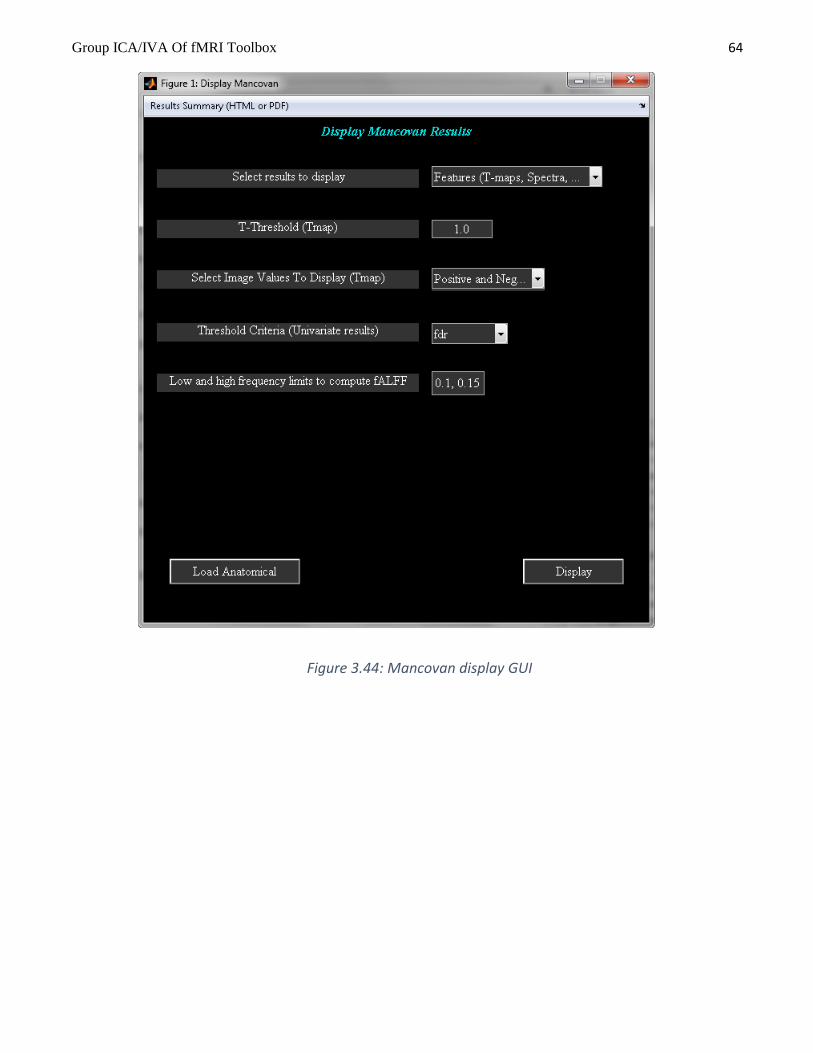
Group ICA/IVA Of fMRI Toolbox 64
Figure 3.44: Mancovan display GUI

Group ICA/IVA Of fMRI Toolbox 65
Figure 3.45: T-map and Spectra
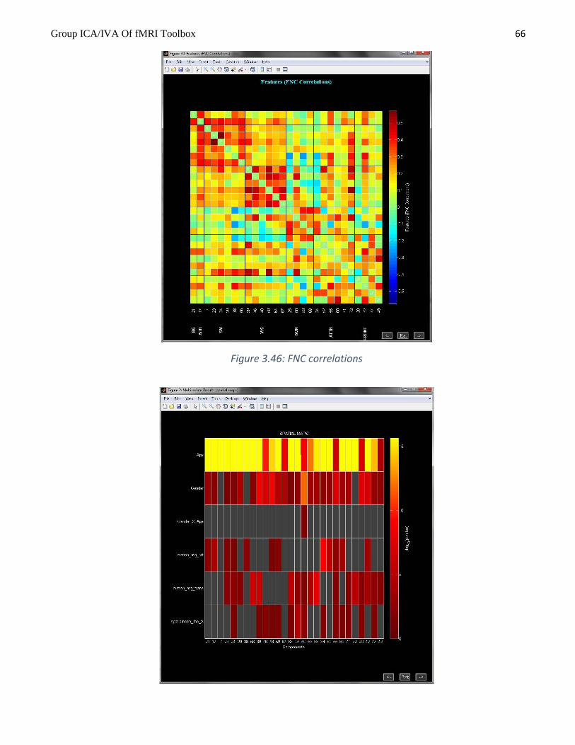
Group ICA/IVA Of fMRI Toolbox 66
Figure 3.46: FNC correlations

Group ICA/IVA Of fMRI Toolbox 67
Figure 3.47: Multivariate Results
Figure 3.48: Spatial maps univariate results

Group ICA/IVA Of fMRI Toolbox 68
3.49: FNC univariate results

Group ICA/IVA Of fMRI Toolbox 69
3.50: Connectogram of FNC univariate results

Group ICA/IVA Of fMRI Toolbox 70
Figure 3.51: Spectra univariate results

Group ICA/IVA Of fMRI Toolbox 71
Figure 3.52: Temporal dFNC Toolbox
Figure 3.53: Temporal dFNC Setup Analysis
Figure 3.54: Temporal dFNC Defaults
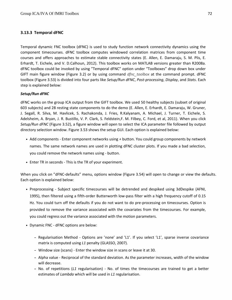
Group ICA/IVA Of fMRI Toolbox 72
3.13.3 Temporal dFNC
Temporal dynamic FNC toolbox (dFNC) is used to study function network connectivity dynamics using the
component timecourses. dFNC toolbox computes windowed correlation matrices from component time
courses and offers approaches to estimate stable connectivity states (E. Allen, E. Damaraju, S. M. Plis, E.
Erhardt, T. Eichele, and V. D.Calhoun, 2012). This toolbox works on MATLAB versions greater than R2008a.
dFNC toolbox could be invoked by using ”Temporal dFNC” option under “Toolboxes” drop down box under
GIFT main figure window (Figure 3.2) or by using command dfnc_toolbox at the command prompt. dFNC
toolbox (Figure 3.53) is divided into four parts like Setup/Run dFNC, Post-processing, Display, and Stats. Each
step is explained below:
Setup/Run dFNC
dFNC works on the group ICA output from the GIFT toolbox. We used 50 healthy subjects (subset of original
603 subjects) and 28 resting state components to do the demo (E. Allen, E. Erhardt, E. Damaraju, W. Gruner,
J. Segall, R. Silva, M. Havlicek, S. Rachakonda, J. Fries, R.Kalyanam, A. Michael, J. Turner, T. Eichele, S.
Adelsheim, A. Bryan, J. R. Bustillo, V. P. Clark, S. Feldstein,F. M. Filbey, C. Ford, et al, 2011). When you click
Setup/Run dFNC (Figure 3.52), a figure window will open to select the ICA parameter file followed by output
directory selection window. Figure 3.53 shows the setup GUI. Each option is explained below:
• Add components - Enter component networks using + button. You could group components by network
names. The same network names are used in plotting dFNC cluster plots. If you made a bad selection,
you could remove the network names using - button.
• Enter TR in seconds - This is the TR of your experiment.
When you click on ”dFNC-defaults” menu, options window (Figure 3.54) will open to change or view the defaults.
Each option is explained below:
• Preprocessing - Subject specific timecourses will be detrended and despiked using 3dDespike (AFNI,
1995), then filtered using a fifth-order Butterworth low-pass filter with a high frequency cutoff of 0.15
Hz. You could turn off the defaults if you do not want to do pre-processing on timecourses. Option is
provided to remove the variance associated with the covariates from the timecourses. For example,
you could regress out the variance associated with the motion parameters.
• Dynamic FNC - dFNC options are below:
– Regularisation Method - Options are ’none’ and ’L1’. If you select ’L1’, sparse inverse covariance
matrix is computed using L1 penalty (GLASSO, 2007).
– Window size (scans) - Enter the window size in scans or leave it at 30.
– Alpha value - Reciprocal of the standard deviation. As the parameter increases, width of the window
will decrease.
– No. of repetitions (L1 regularisation) - No. of times the timecourses are trained to get a better
estimates of Lambda which will be used in L1 regularisation.

Group ICA/IVA Of fMRI Toolbox 73
After completing the parameters selection, use Run (Figure 3.53) to run the dynamic FNC. Windowed
correlation matrices are saved for each subject in variable FNCdyn in file prefix_sub_*_results.mat. dFNC
parameters are saved in variable dfncInfo in file prefix_dfnc.mat where prefix is the same prefix you gave
during the ICA analysis.
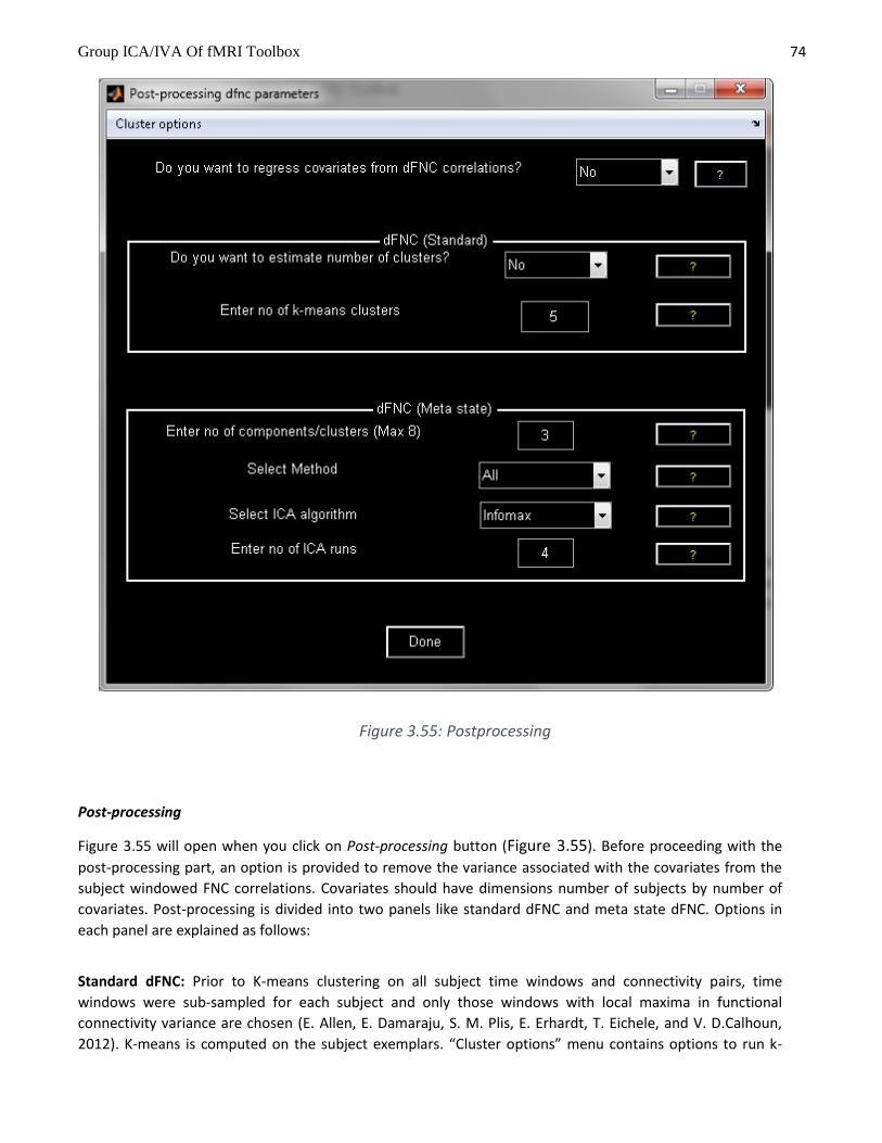
Group ICA/IVA Of fMRI Toolbox 74
Figure 3.55: Postprocessing
Post-processing
Figure 3.55 will open when you click on Post-processing button (Figure 3.55). Before proceeding with the
post-processing part, an option is provided to remove the variance associated with the covariates from the
subject windowed FNC correlations. Covariates should have dimensions number of subjects by number of
covariates. Post-processing is divided into two panels like standard dFNC and meta state dFNC. Options in
each panel are explained as follows:
Standard dFNC: Prior to K-means clustering on all subject time windows and connectivity pairs, time
windows were sub-sampled for each subject and only those windows with local maxima in functional
connectivity variance are chosen (E. Allen, E. Damaraju, S. M. Plis, E. Erhardt, T. Eichele, and V. D.Calhoun,
2012). K-means is computed on the subject exemplars. “Cluster options” menu contains options to run k-

Group ICA/IVA Of fMRI Toolbox 75
means multiple times, change distance metric, set maximum number of iterations and number of reference
data-sets for using gap statistic. Option is provided to estimate the number of clusters using Gap statistic and
Silhouette algorithms. To speed up the process, estimate clusters step is done only on the subject exemplars.
If you skip this part, enter the number of k-means clusters in the edit box. Resulting centroids are used in the
initialization of k-means on the windowed FNC correlations across all subjects.
Meta states dFNC: Meta state dynamics method (Robyn L. Miller, 2016) relies on reducing the number of
windowed FNC correlations to a few components/clusters using methods like k-means, temporal ICA, spatial
ICA and PCA (User specified). Dynamic FNC correlations are basically factorized into continuous loading
coefficients or timecourses and connectivity patterns. Resulting continuous loading coefficients are
discretized using quartile discretization and are of dimensions windows by number of clusters by subjects.
The following metrics are performed on the discretized loading coefficients:
Number of states: Number of unique windows for each subject.
Change of states: Number of times each subject changes from one meta state to other.
State span: Maximum L1 distance between states for each subject.
Total distance: Sum of L1 distances between successive meta-states for each subject.
At the end of the post-processing step, results are saved in file _post_process.mat. Meta state analysis
information is saved in field “meta_states_info”.
Note: Please note that k-means in meta state analysis uses random initialization and also you could select
different number of clusters for each dFNC panel.
Display
Display GUI includes options to display FNC spectra, cluster centroids and meta states. When you click on
Display button (Figure 3.52), display window (Figure 3.56) will open. There are two options like ”FNC
Oscillations and ”Cluster stats”.
FNC Oscillations - Average standard deviation of spectra and average spectral central of mass are
computed. Figure 3.57 shows the average standard deviation of FNC spectra across subjects.
Cluster stats - K-means is computed on the windowed correlations and 6 clusters are selected. Figure
3.58 shows one of the cluster centroids. Title shows percentage of number of occurrences of the
cluster over the total number of occurrences. Figure 3.59 shows the frequency of each cluster, mean
dwell time in windows for each cluster and state transition matrix. State vector for each subject is
displayed is shown in Figure 3.60.
Meta state analysis: Connectivity patterns of the selected method in the post-process GUI will be
shown similar to Figure 3.58.

Group ICA/IVA Of fMRI Toolbox 76
Note: HTML report is created in html directory when you click on ”HTML” menu in display GUI shown below.
Figure 3.56: Display dFNC Results

Group ICA/IVA Of fMRI Toolbox 77
Figure 3.57: Average standard deviation of FNC Spectra across subjects
Figure 3.58: Cluster centroid
Figure 3.59: State Vector Stats

Group ICA/IVA Of fMRI Toolbox 78
Figure 3.60: State vector for each subject
Stats
Option is now provided to compute statistics on median of dFNC correlations when you click on Stats button (Figure
3.52). The following are the parameters in Figure 3.61:
“Select design criteria” – Options are “one sample t-test”, “two sample t-test” and “paired t-test”. When you select
the design criteria, you have the option to specify subjects used in the calculation.
“Enter threshold in windows” - For each subject, median of dFNC correlations across windows is computed. Only
those subjects are included in the stats which have at least the threshold in number of windows specified. When you
click on “Calculate” button, t-test results are written to file with suffix ttest_results.mat. Median of dFNC
correlations and state vector stats information is written to file with suffix cluster_stats.mat. To view the results in a
web browser, click on “HTML results” menu (Figure 3.61).
Note: T-tests are done on meta-state metrics and also summarized in the HTML report. Option to use select
threshold criteria (FDR or un-corrected) and threshold are available in “Stats-Defaults” menu.
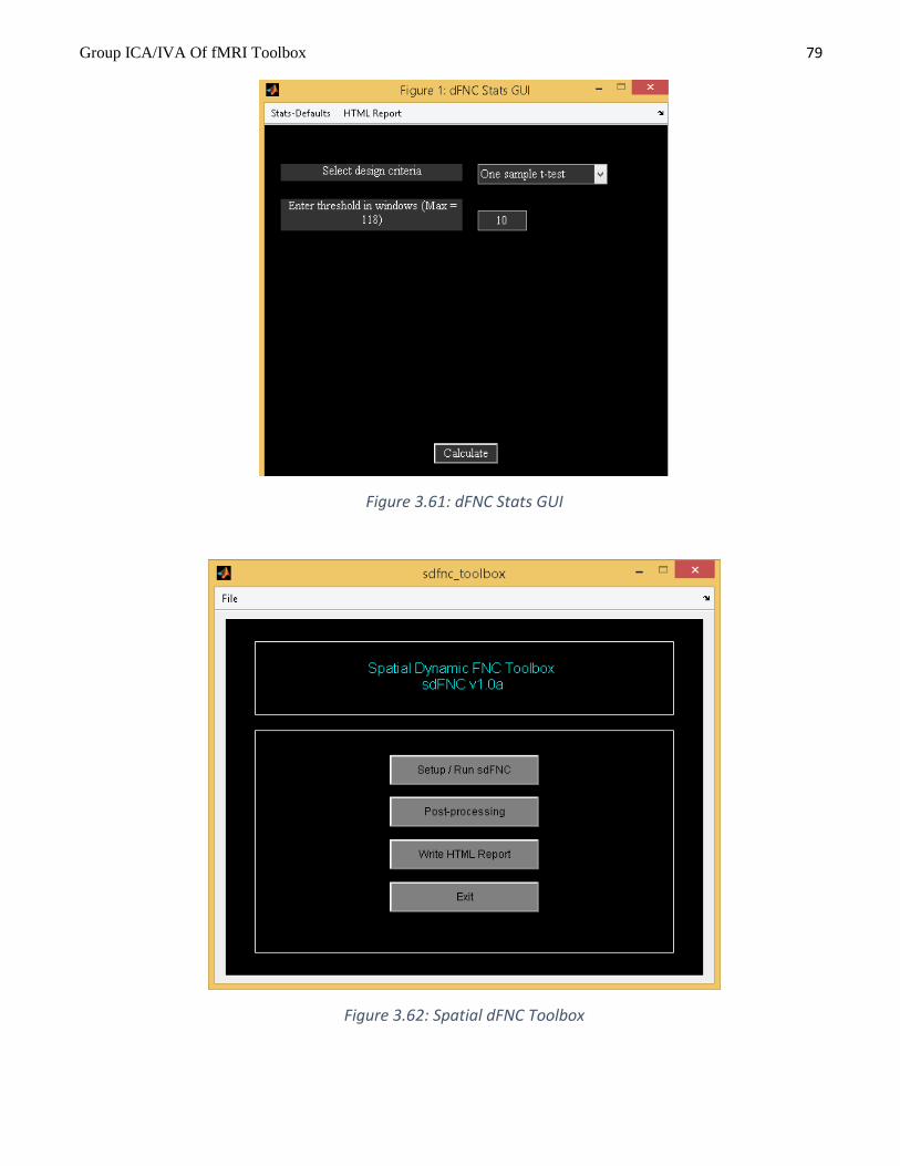
Group ICA/IVA Of fMRI Toolbox 79
Figure 3.61: dFNC Stats GUI
Figure 3.62: Spatial dFNC Toolbox

Group ICA/IVA Of fMRI Toolbox 80
Figure 3.63: Setup spatial dFNC
3.13.4 Spatial dFNC
We now provide an option to do dynamic functional connectivity using the component maps. Spatial dFNC toolbox is
based on paper (S. Ma, V. Calhoun, R. Phlypo and T. Adali, 2014) . We provide a brief description of the method
below:
Method: Sliding windows are used to divide total time points for each subject into smaller data sets. IVA-GL
algorithm is applied on all these smaller data sets for all subjects. Back-reconstructed component maps are
obtained for each subject at each time window.
Post-processing:
o For each subject at each window, mutual information (spatial connectivity) is computed between all
possible pairs of spatial maps.
o Standard deviation of functional connectivity across windows is calculated for each subject. Mann-
Whitney U-test is used to examine if there is significant group difference.
o For each component, connectivity values with other components are used to perform Markov
modeling. Connectivity values are used as features to perform K-means clustering and each cluster
represents one state in Markov chain. State transition is computed for each subject at all windows.
To invoke spatial dFNC toolbox (sDFNC), click on “Spatial dFNC” under “Toolboxes” drop down box (Figure 3.2).
Toolbox (Figure 3.62) is divided into Setup/Run sDFNC, Post-processing and Write HTML Report. Each option is
discussed below:
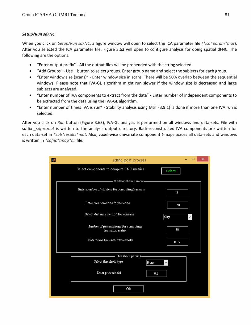
Group ICA/IVA Of fMRI Toolbox 81
Setup/Run sdFNC
When you click on Setup/Run sdFNC, a figure window will open to select the ICA parameter file (*ica*param*mat).
After you selected the ICA parameter file, Figure 3.63 will open to configure analysis for doing spatial dFNC. The
following are the options:
“Enter output prefix” - All the output files will be prepended with the string selected.
“Add Groups” - Use + button to select groups. Enter group name and select the subjects for each group.
“Enter window size (scans)” - Enter window size in scans. There will be 50% overlap between the sequential
windows. Please note that IVA-GL algorithm might run slower if the window size is decreased and large
subjects are analyzed.
“Enter number of IVA components to extract from the data” - Enter number of independent components to
be extracted from the data using the IVA-GL algorithm.
“Enter number of times IVA is run” - Stability analysis using MST (3.9.1) is done if more than one IVA run is
selected.
After you click on Run button (Figure 3.63), IVA-GL analysis is performed on all windows and data-sets. File with
suffix _sdfnc.mat is written to the analysis output directory. Back-reconstructed IVA components are written for
each data-set in *sub*results*mat. Also, voxel-wise univariate component t-maps across all data-sets and windows
is written in *sdfnc*tmap*nii file.

Group ICA/IVA Of fMRI Toolbox 82
Figure 3.64: Spatial dFNC Post-processing GUI
Post-processing
When you click on post-processing button (Figure 3.62) and select the spatial dFNC information file (*sdfnc.mat),
Figure 3.64 will open to do post-processing as discussed in setup analysis. You need to select components of interest
using the Select button. Option is provided to enter Markov modeling parameters and threshold for doing t-tests.
After you click on Ok button, post-processing results are saved in file with suffix *sdfnc_post_process.mat. Variables
stored in post-processing results file are as follows:
KL – Kullback-Liebler (KL) divergence is computed between sequential windows for each group in a cell array.
Each cell is of dimensions number of subjects in current group by number of windows - 1.
MI – Mutual information is computed for each component pair for all subjects, sessions and windows.
Dimensions of variable are components by components by subjects by sessions by windows.
MIStdVals – Standard deviation across windows is computed for each subject in each group. If there are
sessions, connectivity values are averaged across sessions before computing standard deviation. Dimensions
of each cell are components by components by subjects.
clusterInfo - K-means clustering is computed for each component connectivity values with other
components.
median_test_results – Mann-Whitney U-test is conducted between groups on standard deviation values as
computed in MIStdVals.
ttest_results – Two sample t-test is computed between groups at each window.
Write HTML Report
All the spatial dFNC results discussed above are summarized in HTML page and shown in web browser. Figure 3.65
shows one of the component t-map across all data-sets and windows. T-test results at each window are shown in
Figure 3.66. KL divergence results are summarized in Figure 3.67.
Figure 3.65: T-map across all data-sets and windows

Group ICA/IVA Of fMRI Toolbox 83
Figure 3.66: Two sample t-test between groups at each window
Figure 3.67: KL divergence between sequential windows for each group
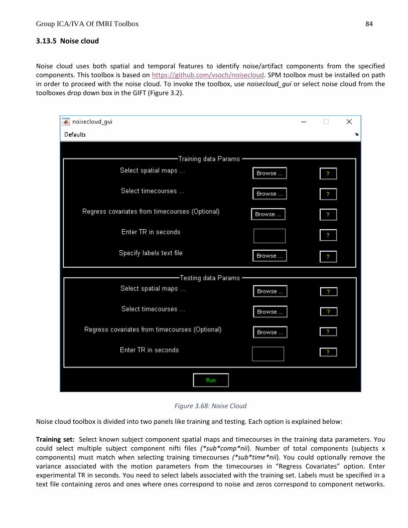
Group ICA/IVA Of fMRI Toolbox 84
3.13.5 Noise cloud
Noise cloud uses both spatial and temporal features to identify noise/artifact components from the specified components. This toolbox is based on https://github.com/vsoch/noisecloud. SPM toolbox must be installed on path in order to proceed with the noise cloud. To invoke the toolbox, use noisecloud_gui or select noise cloud from the toolboxes drop down box in the GIFT (Figure 3.2).
Figure 3.68: Noise Cloud
Noise cloud toolbox is divided into two panels like training and testing. Each option is explained below: Training set: Select known subject component spatial maps and timecourses in the training data parameters. You could select multiple subject component nifti files (*sub*comp*nii). Number of total components (subjects x components) must match when selecting training timecourses (*sub*time*nii). You could optionally remove the variance associated with the motion parameters from the timecourses in “Regress Covariates” option. Enter experimental TR in seconds. You need to select labels associated with the training set. Labels must be specified in a text file containing zeros and ones where ones correspond to noise and zeros correspond to component networks.

Group ICA/IVA Of fMRI Toolbox 85
For example, if you selected 10 subjects each containing 50 components, labels file must contain a vector of length 1 by 500. Testing set: Enter the testing data (component maps and timecourses) which needs to be classified. At the end of the analysis, confusion matrix is shown in the graphical window. Also, results are saved in file “noise_cloud_results.mat”. Variables description is as follows:
class_labels - Contains flags associated with the testing components (Noise or network).
result_nc_classifier - Classifier built using the training data
fit_mdl - Model fit
training_opts - Training options
testing_opts - Testing options Alternatively, you could invoke noise cloud from the command line using the function noisecloud_run. Please see help noisecloud_run or “noisecloud_demo.m” for more details.
3.14 BATCH SCRIPT
3.14.1 Analysis
Batch script is an alternative way to run the group ICA. You could run group ICA in batch in two ways. We discuss below option to run batch script using preference file. Alternative option to run batch script using GICA command line is discussed in Section 3.15. Preference files like Input_spatial_ica.m, Input_data_subjects_1.m and Input_data_subjects_2.m are provided as examples. Input_spatial_ica.m contains preferred settings for performing group ICA. Function for running the batch file is icatb_batch_file_run. The syntax for the function is as given below: Enter icatb_batch_file_run(inputFile) at the MATLAB command prompt where inputFile is the full file path for the input data of the subjects. Batch script and preference files are located in folder icatb_batch_files. Parameters in the preference file are as follows:
perfType - Group PCA performance settings. The best match for each option is dependent on the variable MAX_AVAILABLE_RAM in defaults file. Options are 1, 2 and 3.
o 1 - Maximize performance. o 2 - Use less memory.
o 3 - User specified settings will be selected based on the PCA options.
which_analysis - Options are 1, 2 and 3.
o 1 - Group ICA is run only once. If you have set NUM_RUNS_GICA to more than 1, ICA is run multiple
times and averaged across ICA runs. Better options to do stability analysis are ICASSO or MST.
o 2 - Group ICA is run using ICASSSO. The following are the options available:
icasso_opts.sel_mode - Selection mode. Options are ‘randinit’, ‘bootstrap’ and ‘both’.

Group ICA/IVA Of fMRI Toolbox 86
icasso_opts.num_ica_runs - Number of times you want ICA to be run.
o 3 – Minimum spanning tree approach is used to determine the stable run estimates. You could set
number of ICA runs using mst_opts.num_ica_runs.
dataSelectionMethod - There are four ways to select the data and the SPM design matrix (required for
temporal sorting). Options are 1, 2, 3 and 4. Each option is explained below:
o 1 - Data will be selected automatically if you specify the root folder for subjects and sessions, file
pattern, a flag and file numbers to include. Options for flag are data_in_subject_folder and
data_in_subject_subfolder.
data_in_subject_subfolder - Data is selected from the subject sub-folders. Number of
sessions is equal to the number of sub-folders containing the specified file pattern.
data_in_subject_folder - Data is selected from the subject folders. The number of sessions is
1 and the number of subjects is equal to the number of subject folders containing the
specified file pattern.
spmDesignFilter - Specify design matrix filter pattern here if you have selected
‘diff_sub_diff_sess’ option for variable keyword_designMatrix. It looks for the design matrix in
the respective subject folder or session folders.
o 2 - This option can be used when all the data is not in one directory. You need to specify the data
directory for each subject and session followed by file pattern. The required variables are
selectedSubjects and numOfSess. selectedSubjects contains the names (arbitrary) of subjects (s1
refers to subject1, s2 refers to subject 2, etc) and numOfSess contains the number of sessions.
Subject 1 session 1 data information must be entered in variable s1_s1 and subject 2 session 2
information must be entered in variable s1_s2. Design matrix information must be entered in
_designMat variable.
o 3 - This option uses regular expressions to get the data set directories. The required variables are as
follows:
input_directory_name - Full path of the directory where the subjects and sessions are
located.
subject_dir_regexp - Regular expression used for matching subject directories. This
variable accepts nested paths. For example, to match single slice data in the example
subjects directory, you can use Sub\w+; single\w+ regular expression where semi-colon
is used as a delimiter. If there are no subject directories inside the input directory,
leave it as empty.
session_dir_regexp - Regular expression used for getting the session directories inside
the subject directories. Unlike subject_dir_regexp variable this cannot contain nested
paths. If there are no session directories, leave this as empty.
Note: More information on regular expressions is given in the Appendix 6.5. For a detailed
information about regular expressions, please refer to the MATLAB help.
data_file_pattern - File pattern used for getting data. Use wild card not regular expressions.
file_numbers_to_include - This option will let you work on a subset of files. Enter the file
numbers to include. Leave it as empty if you want to include all the files.

Group ICA/IVA Of fMRI Toolbox 87
spm_stats_dir - SPM stats directory name relative to subject or session directories. GIFT will
automatically search in the appropriate directories to get SPM.mat file for the subject.
Please note that this variable will be read only when you use ‘diff_sub_diff_sess’ value for
the variable keyword_designMatrix.
o 4 - This option is useful when you want to specify the file names directly. Each variable is explained
below:
input_data_file_patterns - File patterns in a cell of dimensions equal to number of subjects
and sessions. Each new subject must be entered in a new row.
input_design_matrices - This variable will be read only when you are using a different design
between subjects and sessions.
dummy_scans - Enter number of dummy scans to exclude from the analysis.
keyword_designMatrix - Design matrix is used for sorting the components temporally during display and will
not be used during the analysis stage except for semi-blind ICA. There are four options like ‘no’,
‘same_sub_same_sess’, ‘same_sub_diff_sess’ and ‘diff_sub_diff_sess’.
o ‘no’ - SPM design matrix is not specified for the analysis.
o ‘same_sub_same_sess’ - All the subjects and sessions will share the same regressors. Specify
location of the SPM design matrix in variable OnedesignMat.
o ‘same_sub_diff_sess’ - Different regressors can be specified over sessions but same over subjects.
Specify location of the SPM design matrix in variable OnedesignMat.
o ‘diff_sub_diff_sess’ - Different regressors can be specified over subjects and sessions.
outputDir - Output directory of the analysis.
prefix - All the output files will be pre-pended with this prefix.
maskFile - Specify the location of the mask file or leave it as empty (Default mask).
preproc_type - Specify type of data pre-processing.
o 1 - ‘Remove mean per time point’
o 2 - ‘Remove mean per voxel’
o 3 - ‘Intensity normalization’
o 4 - ‘Variance normalization’
group_pca_type - Select the type of group PCA.
o ’subject specific’ - Subject specific
o ’grand mean’ - Grand mean
pcaType - Specify PCA type.
o 1 - ‘Standard’
o 2 - ‘Expectation Maximization’
o 3 - ‘SVD’
o 4 - ‘MPOWIT’
o 5 - ‘STP’
pca_opts - Optional parameters for PCA.
o ‘Standard’:
pca_opts.stack_data - Options are as follows:
- ’Yes’ - Data sets are stacked to compute covariance matrix. This option assumes that
there is enough RAM to stack the data sets and for computing the covariance
matrix. Full storage of covariance matrix is used.

Group ICA/IVA Of fMRI Toolbox 88
- ’No’ - A pair of data sets are loaded at a time to compute covariance matrix.
This option uses less memory usage but slower than the other option. You also
have the option to store only the lower triangular portion of the covariance
matrix (packed storage) when using this option.
pca_opts.storage - Options are ’Full’ and ’Packed’. Packed storage scheme uses only lower
triangular portion of symmetric matrix to compute eigen values.
pca_opts.precision - Options are ’Double’ and ’Single’. Single precision is accurate up to 7
digits after decimal place and uses 50% less memory usage when compared to double
precision.
pca_opts.eig_solver - Options are ’Selective’ and ’All’. These options will be used only
when you use packed storage scheme. Use option ’All’ only when there are convergence
issues with the option ’Selective’.
‘Expectation Maximization’:
o pca_opts.stack_data - Options are as follows:
’Yes’ - This option assumes that there is enough RAM to stack the data sets.
’No’ - A data-set is loaded at a time to compute the transformation matrix.
o pca_opts.precision - Options are ’Double’ and ’Single’.
o pca_opts.tolerance - Enter stopping tolerance. Default is 1e-4.
o pca_opts.max_iter - Enter maximum number of iterations to use.
‘SVD’:
o pca_opts.precision - Options are ’Double’ and ’Single’.
o pca_opts.solver - Options are ’Selective’ and ’All’.
‘MPOWIT’:
o pca_opts.stack_data - Options are as follows:
’Yes’ - This option assumes that there is enough RAM to stack the data sets.
’No’ - A data-set is loaded at a time to solve the eigen value problem.
o pca_opts.precision - Options are ’Double’ and ’Single’.
o pca_opts.tolerance - Enter stopping tolerance. Default is 1e-6.
o pca_opts.max_iter - Enter maximum number of iterations to use.
o pca_opts.block_multiplier - Enter block multiplier. Default is set to 10.
‘STP’:
o pca_opts.precision - Options are ’Double’ and ’Single’.
o pca_opts.num_comp - Enter number of intermediate components to retain. Default is set to 500.
o pca_opts.numGroups - Number of subjects in each group. Default is set to 10.
backReconType - Options are 1, 2, 3 and 4.
o 1 - Regular
o 2 - Spatial-temporal regression
o 3 - GICA3
o 4 - GICA

Group ICA/IVA Of fMRI Toolbox 89
numReductionSteps - The number of reduction steps used and is dependent on the number of data-sets
used. A maximum of two reduction steps is used.
doEstimation - 1 means dimensionality estimation is done and PC step numbers are set to this value. You
could select max, mean or median for a particular PC step in variable estimation_opts.
numOfPC1 - Number of PC for reduction step 1.
numOfPC2 - Number of PC for reduction step 2.
scaleType - Options are 0, 1, 2, 3 and 4.
o 0 - No scaling
o 1 - Scale components to percent signal change
o 2 - Z-scores
o 3 - Scaling in timecourses
o 4 - Scaling in maps and timecourses
algoType - Currently, there are 16 ICA/IVA algorithms available in the GIFT toolbox. The algorithms are as
follows:
1 - ‘Infomax’
2 - ‘FastICA’
3 - ‘ERICA’
4 - ‘SIMBEC’
5 - ‘EVD’
6 - ‘JADE OPAC’
7 - ‘AMUSE’
8 - ‘SDD ICA’
9 - ‘Semi-blind ICA’
10 - ‘Constrained ICA (Spatial)’
11 - ‘Radical ICA’
12 - ‘Combi’
13 - ‘ICA-EBM’
14 - ‘ERBM’
15 - ‘IVA-GL’
16 - ‘GIG-ICA’
17 – ‘IVA-L’
refFunNames - Reference function or regressor names to constrain ICA time courses. This is needed when
using semi-blind ICA for the analysis.
refFiles - Spatial reference or template files required to constrain the ICA source maps. This variable is
required when Constrained ICA (Spatial) and GIG-ICA algorithms are used for doing ICA. Enter the files in a
cell array.
3.14.2 Display

Group ICA/IVA Of fMRI Toolbox 90
Display methods like Component Explorer, Composite Viewer and Orthogonal Viewer can be accessed through
a batch script. The function for running the batch file is icatb_batch_display. The syntax for the function is as
given below:
Type icatb_batch_display(inputFile) at the MATLAB command prompt where
inputFile is the file containing the necessary display parameters.
The display parameters in the input file are as follows:
• sourceDir - Directory where fMRI images are located.
• sourceFilePattern - File pattern for fMRI images.
• outputDir - Directory where the component images are located.
• compNumbers - Component numbers to plot.
• structFile - All the component images will be overlaid on this anatomical file.
• returnValue - Variable used for plotting activations or deactivations or activations and deactivations on spatial
map. There are four options like 1, 2, 3 and 4.
o 1 - ‘Positive and Negative’
o 2 - ‘Positive’
o 3 - ‘Absolute Value’
o 4 - ‘Negative’
• convertToZ - Convert image values to Z-scores. Options are 1 and 0. 1 means convert to Z-scores.
• thresholdValue - Z-threshold for spatial maps.
• imagesPerFigure - Number of images plotted per figure. Options are 1, 4, 9, 16 and 25.
• anatomicalPlane - Slice plane used for Component Explorer or Composite Viewer display methods. Options
used are ’axial’, ’sagittal’ and ’coronal’.
• displayType - Display method to use. Options are ’component explorer’, ’composite viewer’ and ’orthogonal
viewer’.
3.14.3 Stats On Beta Weights
Statistics on beta weights can also be done using a batch script. Example batch file
(Input_data_stats_beta_weights.m) is in folder icatb/icatb_batch_files. The parameters in the batch file are as
follows:

Group ICA/IVA Of fMRI Toolbox 91
• averageRuns - A value of 1 means beta weights will be averaged across runs or sessions. The number of
sessions will be set to 1.
• desCriteria - Design criteria used to test the significance of components. There are six options like:
– 1 - One sample t-test
– 2 - Two sample t-test
– 3 - One way anova between the groups
– 4 - One way anova between the regressors
– 5 - Two way anova where groups and regressors are used as independent variables
– 6 - Multiple Regression
• groupInfo - Variable containing information about the groups. This variable must be a cell array of size number
of groups by 3. Each row must contain a name for group, subject numbers and session numbers. You can also
use commands like load(’c:\healthy.asc’) in place of subject or session numbers.
• selGroups - Groups used for doing statistics on beta weights.
• selConditions - Regressors used for doing statistics on beta weights.
• multi_regress_files - You can specify regressor files like age, test scores, etc in a cell array. The format for the
text files is ASCII or MAT.
• eq_regressors - This option is provided when one way anova (groups) design criteria is selected. For example,
you could do a one way anova between groups by subtracting one condition from another.
• contrastNames - A cell array containing contrast names.
• contrastMatrix - Each row of contrast matrix must equal to zero. The number of contrasts must equal the
number of rows of contrast matrix. Contrast matrix depends on the design criteria selected. The description is
as follows:
– One way anova (groups) - The length of contrast vector must equal the number of selected groups like
[g1, g2, etc].
– One way anova (regressors) - The length of contrast vector must equal the number of selected regressors
or conditions like [c1, c2, c3, c4, etc].
– Two way anova (groups, regressors) - The length of contrast vector must equal the number of selected
groups and regressors like [g1, g2, c1, c2, c3, c4, etc].
After entering the values for the variables in a batch file, type the following at the MATLAB command prompt:
icatb_statistical_testing_TC(regressParamFile, userInputFile); where regressParamFile is the regression parameters
text file and userInputFile is the batch file.

Group ICA/IVA Of fMRI Toolbox 92
3.14.4 Mancovan
Batch template for mancova is located at icatb\icatb_batch_files\input_mancovan.m. The following are the
variables:
• outputDir - Output directory to place the analysis results.
• ica_param_file - Full path to ICA parameter file.
• features - Options are spatial maps, timecourses spectra and FNC correlations.
• covariates - Enter covariates information in a cell array of dimensions no. of covariates by 4. The four columns
are covariate name, type, vector and transformation function. You could use file name instead of entering
covariate vector. This file must be ascii for continuous covariates and a text file with new line, comma or tab as
delimiter for categorical covariates. Transformation function will be used only for continuous covariates.
• interactions - Specify pairwise model interactions. If you don’t want to use interactions, you could leave it as
empty.
• comp_network_names - Component networks. Enter name followed by values where values are component
numbers. The names information will be used in future release for advanced plotting.
• numOfPCs - Number of principal components used to reduce the data in voxel or spectra dimension which will
be used in multivariate tests. The vector length must match the no. of features.
• p_threshold - Significance threshold used in multivariate and univariate tests.
• TR - TR of the experiment in seconds.
After entering the parameters, use icatb_mancovan_batch(inputFile); at the command prompt.
3.14.5 Temporal dFNC
Batch template for temporal dFNC is located at icatb\icatb_batch_files\input_dfnc.m. The following are the
variables:
• outputDir - Output directory to place the analysis results.
• ica_param_file - Full path to ICA parameter file.
• comp_network_names - Component networks. Enter name followed by values where values are component
numbers. The names information will be used in future release for advanced plotting.

Group ICA/IVA Of fMRI Toolbox 93
• TR - TR of the experiment in seconds.
• dfnc_params – Parameters used for despiking and filtering. Option is also provided to use L1 regularization
when computing dFNC correlations.
3.15 GICA COMMAND LINE
Option is now provided to run group ICA in batch mode using minimum number of input parameters. Each option
should be preceded with “--“ prefix. Please use “help gica_cmd” at the MATLAB prompt for more information. Some
examples are shown below:
“gica_cmd --data ‘C:\sub001.nii’ ‘C:\sub002.nii’” - Runs standard group ICA using two data reductions and
Infomax algorithm. Since the number of components is not provided, MDL dimensionality estimation tool is
used to determine the number of components. Note you could also specify text file containing Nifti file
names instead of entering file names by hand (“gica_cmd --data ‘C:\files.txt’ ”).
“gica_cmd -- data ‘C:\sub001.nii’ --n 15 --a combi” - Number of components is set to 15 and algorithm is set
to Combi.
“gica_cmd --data ‘C:\sub001.nii’ ‘C:\sub002.nii’ ‘C:\sub003.nii’ --n 20 --reductions 1” - Runs group ICA on
multiple data-sets using one data reduction step i.e., the group PCA is directly done on the stacked pre-
processed data.
“gica_cmd --data ‘C:\sub001.nii’ ‘C:\sub002.nii’ ‘C:\sub003.nii’ --templates ‘C:\spatial_ref.nii’ --a gig-ica ” -
Runs constrained spatial algorithm GIG-ICA using the given spatial reference Nifti files.
“gica_cmd --data ‘C:\sub001.nii’ --icasso 5 --o ‘C:\tmp’ ” - ICASSO is run five times on the Infomax algorithm.
Results are written to specified output directory to ‘C:\tmp’.
“gica_cmd --data ‘C:\files.txt’ --n 30 --reductions 2 --parallel 4” - Large data-sets are run in parallel using the
specified number of MATLAB workers after the “--parallel” prefix.
3.16 OUTPUT FILES NAMING
• Parameter file - File used for storing parameters before and after the analysis. _ica_parameter_info.mat
is the suffix used for parameter file.
• Reduction step file - After PCA, the information is stored in a MAT file. _pca_r is the suffix used for
reduction files.
• ICA step file - After ICA, the information is stored in a MAT file with the suffix _ica. The aggregate
images are written in Analyze or Nifti format with the suffix _agg__component_ica_.
• Back reconstruction step file - After back reconstruction step, the information is stored in a MAT file
with the suffix _ica_br.

Group ICA/IVA Of fMRI Toolbox 94
• Calibrate step file - After scaling, the information is stored in a MAT file with the suffix _ica_c.
• Component map file - Component maps are stored with the suffix _component_ica_ in Analyze or Nifti
format. Subject component maps are stored as *sub*component_ica*nii.
• Component time course file - Component time course for a particular data-set is stored with the suffix
_timecourses_ica_ in Analyze or Nifti format.
Note: To load the image files, use icatb_loadData(file_name).
Figure 3.69: Source Based Morphometry
3.17 SOURCE BASED MORPHOMETRY
Source Based Morphometry (SBM) is a multivariate tool to study the gray matter differences between
the patients and controls (A. Caprihan, C. Abbott, J. Yamamoto, G. D. Pearlson, N. Bizzozero, J. Sui, and
V. D. Calhoun, 2011) and (L. Xu, K. Groth, G. Pearlson, D. Schretlen, and V. Calhoun, 2009). ICA is used
on the subject images to determine the maximally independent sources. Basically ICA decomposes
data into subject loading coefficients and component maps. It is similar to doing single subject single
session analysis in the GIFT except the timepoints are subject images. To invoke SBM (Figure 3.69),
type sbm or groupica smri at the MATLAB command prompt. The following are the differences
between the GIFT and SBM:
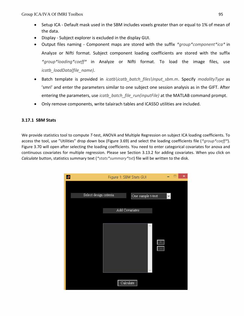
Group ICA/IVA Of fMRI Toolbox 95
Setup ICA - Default mask used in the SBM includes voxels greater than or equal to 1% of mean of
the data.
Display - Subject explorer is excluded in the display GUI.
Output files naming - Component maps are stored with the suffix *group*component*ica* in
Analyze or Nifti format. Subject component loading coefficients are stored with the suffix
*group*loading*coeff* in Analyze or Nifti format. To load the image files, use
icatb_loadData(file_name).
Batch template is provided in icatb\icatb_batch_files\Input_sbm.m. Specify modalityType as
’smri’ and enter the parameters similar to one subject one session analysis as in the GIFT. After
entering the parameters, use icatb_batch_file_run(inputFile) at the MATLAB command prompt.
Only remove components, write talairach tables and ICASSO utilities are included.
3.17.1 SBM Stats
We provide statistics tool to compute T-test, ANOVA and Multiple Regression on subject ICA loading coefficients. To
access the tool, use ”Utilities” drop down box (Figure 3.69) and select the loading coefficients file (*group*coeff*).
Figure 3.70 will open after selecting the loading coefficients. You need to enter categorical covariates for anova and
continuous covariates for multiple regression. Please see Section 3.13.2 for adding covariates. When you click on
Calculate button, statistics summary text (*stats*summary*txt) file will be written to the disk.
Group ICA/IVA Of fMRI Toolbox 96
Figure 3.70: SBM Stats GUI
3.18 INDEPENDENT VECTOR ANALYSIS
IVA-GL is based on a two-step procedure using IVA with multivariate Gaussian priors (IVA-G) (M. Anderson, T. Adali
and X.-L. Li, 2012) and IVA algorithm with a Laplacian prior (T. Kim, H. T. Attias, S.-Y. Lee, and T.-W. Lee, 2007). IVA-
GL uses only a single subject level PCA step and is shown to provide good performance in capturing extreme subject
variability (S. Ma, R.Phlypo, V.D. Calhoun, and T. Adali, 2013) and (J. T. Dea, M. Anderson, E. Allen, V. D. Calhoun, and
T. Adali, 2011). We used 3 subjects and 1 session from Visuomotor data and extracted 16 components. Figure 3.71
shows top 4 components ranked based on temporal regression value (R2).
Note: When analyzing large data-sets computational time and memory will impact the performance of IVA-GL
algorithm. To handle this, you could use IVA-L algorithm. By default, weights are initialized using weights from the
group PCA. We confirm our findings using a simulated data-set (Figure 3.72). Top row shows individual subject
components from a simulation and estimated subject components using IVA-GL. Bottom row shows components
estimated using IVA-L algorithm with group PCA initialization. IVA-L using weights from the group PCA is comparable
to IVA-GL (Figure 3.72).
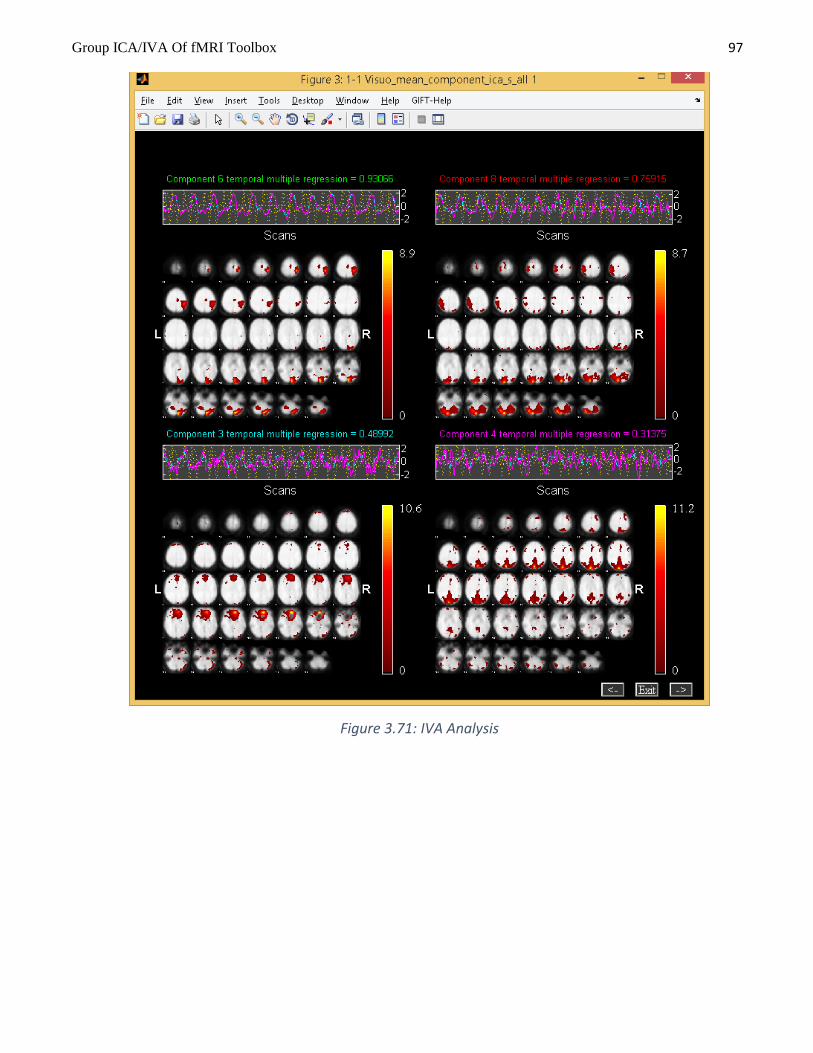
Group ICA/IVA Of fMRI Toolbox 97
Figure 3.71: IVA Analysis

Group ICA/IVA Of fMRI Toolbox 98
3.72: IVA Simulation
3.19 DISPLAY TOOLS
Display tools like ‘Image Viewer’, ‘Component Explorer’, ‘Composite Viewer’, ‘Orthogonal Explorer’,
‘Component Viewer’ and ‘Group Networks’ are available. ‘Component Explorer’, ‘Orthogonal Explorer’ and
‘Component Viewer’ are standalone tools and are independent of the ICA parameter file. For specific
details about the display parameters, please see Section 3.10.1. We discuss below ‘Image Viewer’,
‘Component Viewer’ and ‘Group Networks’:
3.19.1 Image Viewer
Options to do image rendering and displaying components as montage or as orthogonal slices are provided. You also
have the option to use composite plot. Figure 3.73 will open when you click on ‘Image Viewer’ in ‘Display Tools’
(Figure 3.2) and select file to display. Display parameters are the same as described in Section 3.10.1. We selected
‘Render’ for option “Select display type”. By default, templated selected for rendering is
icatb_templates\render_single_subj.mat (Statistical Parameteric Mapping, 1991). It is advised not to convert images
to Z-scores if you are using T-maps. Figure 3.74 shows two task-related components and a transiently task related
component from visuomotor task in a composite plot. Also, orthogonal slices are shown in Figure 3.75. You could
also invoke ‘Image Viewer’ using the following commands:
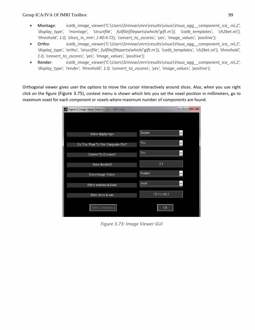
Group ICA/IVA Of fMRI Toolbox 99
Montage: icatb_image_viewer('C:\Users\Srinivas\mrn\results\visuo\Visuo_agg__component_ica_.nii,2',
'display_type', 'montage', 'structfile', fullfile(fileparts(which('gift.m')), 'icatb_templates', 'ch2bet.nii'),
'threshold', 1.0, 'slices_in_mm', (-40:4:72), 'convert_to_zscores', 'yes', 'image_values', 'positive');
Ortho: icatb_image_viewer('C:\Users\Srinivas\mrn\results\visuo\Visuo_agg__component_ica_.nii,2',
'display_type', 'ortho', 'structfile', fullfile(fileparts(which('gift.m')), 'icatb_templates', 'ch2bet.nii'), 'threshold',
1.0, 'convert_to_zscores', 'yes', 'image_values', 'positive');
Render: icatb_image_viewer('C:\Users\Srinivas\mrn\results\visuo\Visuo_agg__component_ica_.nii,2',
'display_type', 'render', 'threshold', 1.0, 'convert_to_zscores', 'yes', 'image_values', 'positive');
Orthogonal viewer gives user the options to move the cursor interactively around slices. Also, when you use right
click on the figure (Figure 3.75), context menu is shown which lets you set the voxel position in millimeters, go to
maximum voxel for each component or voxels where maximum number of components are found.
Figure 3.73: Image Viewer GUI
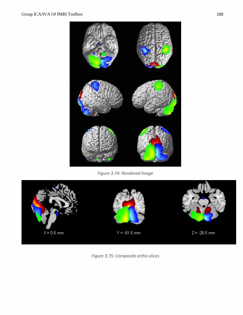
Group ICA/IVA Of fMRI Toolbox 100
Figure 3.74: Rendered Image
Figure 3.75: Composite ortho-slices

Group ICA/IVA Of fMRI Toolbox 101
Figure 3.76: Component Viewer GUI
3.19.2 Component Viewer
Component viewer displays orthogonal slices of the selected viewing set and mean with standard error of mean of
spectra across data-sets (Figure 3.77). The following GUI (Figure 3.76) will open when you selected the anatomical
file to overlay components and selected the viewing set. Display parameters are similar to display GUI parameters
(3.10.1). We explain key options below:
“Enter TR in seconds”: Enter the TR of the experiment in seconds. For accurate results of spectra, you need to use
exact TR.
“Enter Low and High Frequency Limits to compute fALFF” - You need to enter the low and high frequency limits to
compute ratio of low to high frequency power. Power is calculated by computing area under the curve. To compute
low and high frequency power, frequencies less than lower limit and frequencies higher than higher limit are used
respectively.
“Average timecourses across sessions?” - For block design, averaging timecourses across sessions is preferred. If
your design is event related or resting state, it is preferred not to average timecourses across sessions.
“Select Results Format” – Option is now provided to export results to HTML or PDF file.
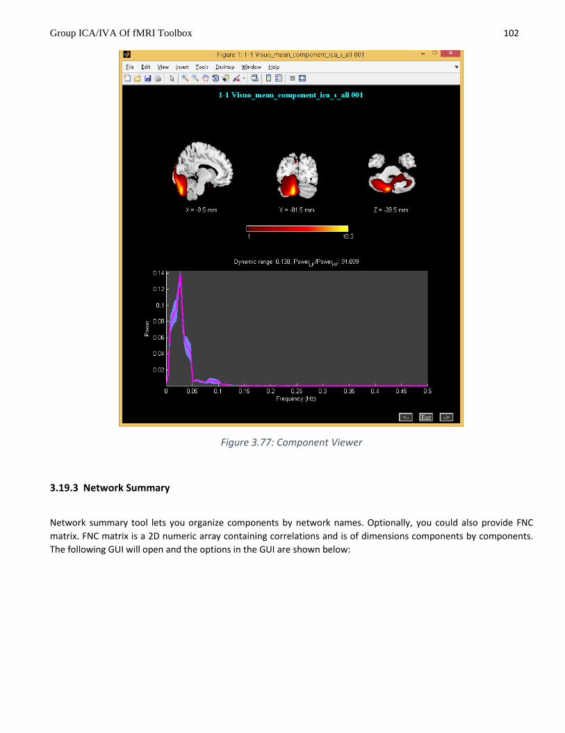
Group ICA/IVA Of fMRI Toolbox 102
Figure 3.77: Component Viewer
3.19.3 Network Summary
Network summary tool lets you organize components by network names. Optionally, you could also provide FNC
matrix. FNC matrix is a 2D numeric array containing correlations and is of dimensions components by components.
The following GUI will open and the options in the GUI are shown below:

Group ICA/IVA Of fMRI Toolbox 103
Figure 3.78: Network summary GUI
Add components: Enter network name and select components corresponding to the network name (Similar
to ‘Add Components’ button in Figure 3.41).
Enter prefix: Results HTML file will be saved with this prefix.
Enter threshold: Enter threshold for spatial maps.
Convert to z-scores: Option is provided to convert component maps to Z-scores.
Select image values: You have the option to display positive, positive and negative, absolute value and
negative values of the spatial maps.
Enter FNC label: Enter a label for FNC correlations which will be used in the matrix and connectogram.
Select anatomical: By default, icatb/icatb_templates/ch2bet.nii file is used as anatomical file for overlaying
the components.
When you click on Ok button, composite rendered plots, composite orthogonal slices, stacked orthogonal slices, FNC
matrix viewer and connectogram1 of FNC correlations are generated. Figures Figure 3.79 and Figure 3.80 show
composite orthogonal views, connectogram of FNC correlations and stacked orthogonal slices.
1 Components are plotted in a circle and are color coded based on the network names. Correlations are plotted using bezier
curves (Komarov, 2013) and color of the curves is based on the colormap defined at the bottom. Component spatial maps are plotted outside the circle in sagittal view.
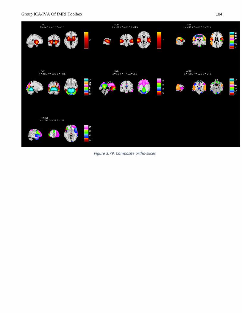
Group ICA/IVA Of fMRI Toolbox 104
Figure 3.79: Composite ortho-slices

Group ICA/IVA Of fMRI Toolbox 105
Figure 3.80: Connectogram of FNC correlations

Group ICA/IVA Of fMRI Toolbox 106
4 PROCESS INVOLVED IN GROUP ICA
In this chapter, the process involved in group ICA is described. This chapter is divided into five sections. Each section is a
step involved in group ICA. In Section 4.1, data reduction step is discussed. In Section 4.2, ICA process and the different
ICA algorithms used in GIFT are explained. In Sections 4.3, brief description about back-reconstruction is included. In
Section 4.4, calibrating the components images and time-courses is discussed. Group statistics on components is
discussed in Section 4.5.
4.1 DATA REDUCTION (PCA)
Data reduction is a step to reduce the size of the subject’s functional data. Principal Components Analysis
(PCA) is used as a technique to reduce the dimensions. At most two data reduction steps are used for multi-
subject analysis.
• One data reduction Step - Group PCA components are directly estimated from the stacked pre-processed
data.
• Two data reduction steps - A single subject might be reduced from 53*63*34*220 to 53*63*34*50. After
each subject’s functional data is reduced, the subjects are then concatenated into one group and put
through another data reduction step.
Note: When using one common data reduction step on multiple subjects, data for each subject needs to be
normalized using intensity normalization or variance normalization. Also, higher number of components
needs to be estimated from the data when compared to two data reduction step.
4.2 INDEPENDENT COMPONENT ANALYSIS
Independent Component Analysis (ICA) is used to find independent components (ICs). GIFT includes a number
of ICA algorithms that are available online and on ICALAB (A. Cichocki, S. Amari, K. Siwek, T. Tanaka, 2003).
Here we briefly introduce some of the ICA algorithms included in GIFT and cite relevant references. We also
discuss a few parameters that affect their separation performance and some of the observations we obtained
in our runs with simulated and real fMRI data (N. Correa, T. Adali, Yi-Ou Li and V. Calhoun, 2005) using
Infomax, FastICA, Jade, SIMBEC and AMUSE.
Infomax uses a fixed sigmoid nonlinearity as the score function and hence emphasizes the estimation of
sources that are super-Gaussian, i.e., have probability density functions (pdfs) that are heavier-tailed and
more peaky than the Gaussian. Hence, the performances of algorithms like Infomax and FastICA that use a
fixed nonlinearity tend to be biased towards certain types of pdfs, in that they provide better estimate for
Group ICA/IVA Of fMRI Toolbox 107
certain classes of sources and hence cannot maximally optimize independence. Algorithms like ICA-EBM
however use a more flexible density model providing more accurate estimation of sources/components with a
broader class of underlying pdfs.
4.2.1 Infomax
Infomax (A. J. Bell and T. J. Sejnowski, 1995) maximizes the information transfer from the input to the output of a
network using a non-linear function. A majority of applications of ICA to fMRI use Infomax since the sources of interest
in this case are super gaussian in nature and the algorithm favors separation of super-gaussian sources. However, the
artifacts present in fMRI data typically have sub-gaussian distributions. To improve separation of the mixture containing
both super-gaussian and sub-gaussian sources, Extended Infomax (T. W. Lee, M. Girolami, and T. J. Sejnowski, 1999) can
be used.
To use Extended Infomax, choose ’1’ instead of the default of ’0’ while selecting ICA options for the Infomax algorithm.
Based on our experiments, we observed that Infomax is a reliable choice for performing ICA on fMRI data. Z-scores for
Infomax were higher than the other algorithms for the task-related source, indicating that Infomax achieves a higher
contrast to noise ratio. Repeated runs showed that the changing initial random condition does not change results
significantly. Infomax is much slower than the other algorithms listed in the toolbox.
4.2.2 Fast ICA
FastICA (A. Hyvarinen and E. Oja, 1997) maximizes the higher order statistics or negentropy of the output to maximize
the non-gaussianity of the estimated sources using fixed point iterations. Two approaches exist: The symmetric
approach estimates all the ICs in parallel and the deflationary approach estimates the ICs one at a time. The tanh, pow3,
gauss and skew non linearities can be used (Hyvarinen, A., 1999).
The desired non-linearity can be chosen while selecting ICA options for FastICA. In our experiments, we used FastICA in
the symmetric mode and compared results obtained using the non linearities tanh, pow3 and gauss. On simulated data,
this algorithm does better in terms of spatial correlation of the estimated sources with the original sources, for super-
gaussian sources when compared to the other sources. For smaller number of components (number of components=5),
FastICA with the gauss non-linearity provides better performance compared to the other two non-linearities for the
gaussian and sub-gaussian sources. However, for a slightly larger simulated set (number of components=8), all three
non-linearities result in very similar performance. Overall, the general performance of FastICA using tanh is better than
the results obtained using the other two non-linearities. For actual fMRI data, we observed that for the transiently task-
related component the spatial extent is slightly higher in FastICA as compared to Infomax. FastICA is slow when it has
convergence problems and in this case it would be advisable to use the stabilized version of the algorithm. This can be
done by changing the stabilization option to ’ON’, while selecting the ICA options.
4.2.3 JADE OPAC
JADE (joint approximate diagonalization of eigenmatrices) (J. F. Cardoso and A. Souloumiac), uses the Jacobi technique,
to perform joint approximate diagonalization on fourth order cumulant matrices to achieve spatial independence
among the sources. The version of JADE included in GIFT is MATLAB optimized with a reduced number of eigen matrices
(A. Cichocki, S. Amari, K. Siwek, T. Tanaka, 2003). JADE is fast and the results are comparable to those obtained using
Group ICA/IVA Of fMRI Toolbox 108
Infomax. In the case of transiently task related components this algorithm shows spatial extent of activations to be
higher than the obtained using Infomax.
4.2.4 SIMBEC
SIMBEC (simultaneous blind extraction using cumulants) (S. Cruces, A. Cichocki and S. Amari, 2001), uses natural
gradient ascent in a Stiefel manifold to simultaneously extract sources using a contrast function based on higher order
cumulants with a learning rate that provides fast convergence.
In our simulations, we observed that for smaller number of components, SIMBEC performs well for the sources of
interest. However, SIMBEC may prove useful to identify the sub-gaussian sources, i.e. artifacts in fMRI data as its
performance for these sources was consistently observed to be very good. SIMBEC is also observed to be one of the
faster algorithms.
4.2.5 AMUSE
AMUSE (algorithm for multiple unknown signal extraction) (L. Tong, V. C. Soon, Y. F. Huang and R. Liu, 1991), is a second
order Blind Source Separation algorithm that utilizes the structure within the data to obtain uncorrelated components.
It performs singular value decomposition on the shifted cross-variance matrix and the shift should be chosen such that
the autocorrelations of the sources at that shift are non-zero and as different from each other as possible. The default
shift is set to ’1’.
AMUSE is highly dependent on the differentiability of the spectra i.e. the autocorrelation of the sources should be
different, for a given delay and its performance suffers greatly when this condition is not met. In our simulations, we
observed that this condition is limiting for fMRI data especially when the number of sources is increased.
4.2.6 ERICA
ERICA (equivariant robust ICA) (S. Cruces, L. Castedo, A. Cichochki, 2000) novel blind source separation algorithms using
cumulants) uses a cumulant based entropy cost function instead of a nonlinearity. The algorithm uses quasi-Newton
iterations and converges at a saddle point of the entropy cost function. The algorithm achieves isotropic convergence, is
fast and is independent of the source distributions regardless of Gaussian noise.
4.2.7 EVD
EVD (eigen value decomposition) algorithm (P. Georgiev and A. Cichocki, 2001) is based on second order statistics and
very similar to AMUSE, the main difference being that EVD uses higher order correlations instead of second order
correlations and is based on non-smooth optimization theory. To achieve separation, the source signals are required to
have linearly independent higher self-correlation functions of even order. The algorithm does not assume non-
gaussianity, non-stationarity and independence.
4.2.8 Constrained ICA (Spatial)

Group ICA/IVA Of fMRI Toolbox 109
Constrained ICA (Q. Lin, J. Liu, Y. Zheng, H. Liang and V. D. Calhoun, 2010) is a semi-blind ICA algorithm that utilizes prior
information about desired sources as reference signals to extract only the desired sources. This algorithm uses fixed
point iteration scheme (fICA-R) for optimizing the constrained ICA contrast function. Compared with the Newton-like
ICA with reference, the fICA-R algorithm has the following advantages:
The fICA-R algorithm has no learning rate and is insensitive to the initialization.
The fICA-R algorithm is simplified since no second derivatives are needed.
The resulting independent components have higher SNR ratio than traditional ICA algorithms.
4.2.9 GIG-ICA
Group information guided ICA (GIG-ICA) (Y. Du, Y. Fan, 2013) uses a no data reduction approach and aggregate
component maps from previous group ICA analysis as reference to estimate sources of interest for each subject.
4.2.10 Real-valued ICA-EBM
ICA by entropy bound minimization (X.-L. Li and T. Adali, Oct 2010) provides flexible density matching through use of
four measuring functions based on the maximum entropy principle. Four nonlinearities are used as measuring functions
for calculating the entropy bound, and the associated maximum entropy density can be symmetric or skewed, heavy-
tailed or not heavy-tailed.
4.2.11 Real-valued ICA-ERBM
ICA by entropy rate bound minimization (X.-L. Li and T. Adali, March 2010) takes both non-Gaussianity and sample
correlation into account by minimizing mutual information rate. It is originally introduced as Full Blind Source
Separation (FBSS). The algorithm by assuming the sources are outputs of linear systems driven by independently and
identically distributed (i.i.d.) noise, the entropy rate estimation problem is converted to an entropy estimation problem
solved using EBM.
4.3 BACK-RECONSTRUCTION
The components resulting from ICA represent group components and therefore, is the motivation for adding the back-reconstruction step. GICA based back-reconstruction methods uses the aggregate components of ICA and the results from data reduction step to compute the individual subject components whereas Spatial-temporal regression approach uses aggregate components and original data to reconstruct individual subject components.
4.4 SCALING COMPONENTS

Group ICA/IVA Of fMRI Toolbox 110
The spatial maps and time courses of components have arbitrary units after the back reconstruction step. Component spatial maps and timecourses can be scaled using percent signal change, Z-scores, scaling in timecourses or scaling in timecourses and maps. It is preferred not to scale components if you have scaled original data using intensity normalization or variance normalization.
4.5 GROUP STATS
Statistics is performed on the group of subjects. Mean, standard deviation and t-maps are calculated on the group of subjects. To give an illustration, let us say M data-sets are used and N components are extracted for each data-set. The mean, standard deviation and t-map are calculated for each component over the number of data-sets used. This will produce N components for mean, standard deviation and t-map.
5 BIBLIOGRAPHY
(1991). Retrieved from Statistical Parameteric Mapping: http://www.fil.ion.ucl.ac.uk/spm/
(1995). Retrieved from AFNI: http://afni.nimh.nih.gov/afni
(1997). Retrieved from EEGLAB Toolbox: http://sccn.ucsd.edu/eeglab/
(2003). Retrieved from ICASSO Toolbox: http://www.cis.hut.fi/projects/ica/icasso/
(2004). Retrieved from MELODIC: http://www.fmrib.ox.ac.uk/fsl/melodic/index.html
(2007). Retrieved from GLASSO: http://cran.r-project.org/web/packages/glasso/
(2011). Retrieved from Chronux: http://chronux.org
A. Caprihan, C. Abbott, J. Yamamoto, G. D. Pearlson, N. Bizzozero, J. Sui, and V. D. Calhoun. (2011). Source-based
morphometry analysis of group differences in fractional anisotropy in schizophrenia. Brain Connectivity, 133-
145.
A. Cichocki, S. Amari, K. Siwek, T. Tanaka. (2003). ICALAB Toolboxes. Retrieved from
http://www.bsp.brain.riken.jp/ICALAB.
A. Garrity, G. D. Pearlson, K. McKiernan, D. Lloyd, K. A. Kiehl, and V. D. Calhoun. (2007). Aberrant default mode
functional connectivity in schizophrenia” Am.J.Psychiatry. Am.J.Psychiatry, 164, 450-457.
A. Hyvarinen and E. Oja. (1997). A fast fixed-point algorithm for independent component analysis. Neural Computing, 9,
1483-1492.
A. J. Bell and T. J. Sejnowski. (1995). An information maximisation approach to blind separation and blind deconvolution.
Neural Computing, 1129-1159.
A. R. Franco, A. Pritchard, V. D. Calhoun, A. R Mayer. (2009). Inter-rater and Inter-method Reliability for Selecting the
Default Mode Network during Data-Driven Analyses. HBM, 30, 2293-2303.

Group ICA/IVA Of fMRI Toolbox 111
E. Allen, E. Damaraju, S. M. Plis, E. Erhardt, T. Eichele, and V. D.Calhoun. (2012). Tracking whole-brain connectivity
dynamics in the resting state. Cereb Cortex.
E. Allen, E. Erhardt, E. Damaraju, W. Gruner, J. Segall, R. Silva, M. Havlicek, S. Rachakonda, J. Fries, R.Kalyanam, A.
Michael, J. Turner, T. Eichele, S. Adelsheim, A. Bryan, J. R. Bustillo, V. P. Clark, S. Feldstein,F. M. Filbey, C. Ford, et
al. (2011). A baseline for the multivariate comparison of resting state networks. Frontiers in Human
Neuroscience.
E. Allen, E. Erhardt, T. Eichele, A. R. Mayer, and V. D. Calhoun. (2010). Comparison of pre-normalization methods on the
accuracy of group ICA results. Barcelona, Spain: HBM.
E. Allen, T. Eichele, L. Wu, and V. D. Calhoun. (2013). EEG Signatures of Functional Connectivity States. Seattle.
E. Erhardt, S. Rachakonda, E. Bedrick, T. Adali, and V. D. Calhoun. (2010). Comparison of multi-subject ICA methods for
analysis of fMRI data. Barcelona, Spain: HBM.
Glahn, D. (2000). SPM fMRI Analysis.
Hyvarinen, A. (1999). Fast and robust fixed-point algorithms for independent component analysis. Neural Networks, 10,
626-634.
J. F. Cardoso and A. Souloumiac. (n.d.). Blind beamforming for non gaussian signals. IEEE, 140(6), 362-370.
J. T. Dea, M. Anderson, E. Allen, V. D. Calhoun, and T. Adali. (2011). IVA for multi- subject fMRI analysis: A comparative
study using a new simulation toolbox. Beijing, China: IEEE Workshop on Machine Learning for Signal Processing
(MLSP).
Knight, J. (2003). Signal Fraction Analysis and Artifact Removal in EEG. Colorado State University, Fort Collins, MS Thesis.
Komarov, O. (2013). Schemaball. Retrieved from https://www.mathworks.com/matlabcentral/fileexchange/42279-
okomarov-schemaball?requestedDomain=www.mathworks.com.
L. Tong, V. C. Soon, Y. F. Huang and R. Liu. (1991). Indeterminacy and identifiability of blind identification. IEEE Trans.
Circuits Sys., 38, 499-509.
L. Xu, K. Groth, G. Pearlson, D. Schretlen, and V. Calhoun. (2009). Source Based Morphometry: The Use of Independent
Component Analysis to Identify Gray Matter Differences with Application to Schizophrenia. HBM, 711-724.
M. Anderson, T. Adali and X.-L. Li. (2012). Joint Blind Source Separation of Multivariate Gaussian Sources: Algorithms
and Performance Analysis. IEEE Trans. Signal Process, 60, 1672-1683.
M. J. McKneown, Scott Makeig, Greg G. Brown, Tzyy-Ping Jung, Sandra S. Kindermann, Anthony J. Bell and Terrence J.
Sejnowski. (1998). Analysis of fMRI Data by Blind Separation Into Independent Spatial Components. HBM, 6,
160-188.
N. Correa, T. Adali, Yi-Ou Li and V. Calhoun. (2005). Comparison of Blind Source Separation algorithms for fMRI. ICASSP,
401-404.
N. Filippini, B. J. MacIntosh, M. G. Hough, G. M. Goodwin, G. B. Frisoni, S. M. Smith, P. M. Matthews, C.F. Beckmann, and
C. E. Mackay. (2009). Distinct patterns of brain activity in young carriers of the APOE-epsilon4. Proc Natl Acad Sci
USA, 106, 7209-7214.
Group ICA/IVA Of fMRI Toolbox 112
P. Georgiev and A. Cichocki. (2001). Blind source separation via symmetric eigenvalue decomposition. Proc. Sixth
International Symposium on Signal Processing and its Applications, Shangri-La Hotel, Kuala Lumpur, Malaysia,
17-20.
Q. Lin, J. Liu, Y. Zheng, H. Liang and V. D. Calhoun. (2010). Semiblind Spatial ICA of fMRI Using Spatial Constraints. HBM,
31(7), 1076-1088.
Robyn L. Miller, M. Y. (2016). Higher Dimensional Meta-State Analysis Reveals Reduced Resting fMRI Connectivity
Dynamism in Schizophrenia Patients. PLOS .
S. Cruces, A. Cichocki and S. Amari. (2001). Criteria for the simultaneous blind extraction of arbitrary groups of sources.
San Diego, California, USA: Int. Conf. Independent Component Analysis and Blind Sig. Separation.
S. Cruces, L. Castedo, A. Cichochki. (2000). Novel blind source separation algorithms using cumulants. IEEE International
Conference on Acoustics, Speech, and Signal Processing, 3152-3155.
S. Ma, R.Phlypo, V.D. Calhoun, and T. Adali. (2013). Capturing group variability using IVA: A simulation study and graph-
theoretical analysis. Vancouver, Canada: IEEE Int. Conf. Acoust., Speech, Signal Processing (ICASSP).
S. Ma, V. Calhoun, R. Phlypo and T. Adali. (2014). Dynamic changes of spatial function network connectivity in healthy
individuals and schizophrenia patients using independent vector analysis. NeuroImage, 90, 196-206.
S.Roweis. (1998). EM algorithms for PCA and sensible PCA. Advances in Neural Information Processing Systems.
T. Kim, H. T. Attias, S.-Y. Lee, and T.-W. Lee. (2007). Blind Source Separation Exploiting Higher-Order Frequency
Dependencies. IEEE Trans. Audio Speech Lang. Process., 15, 70-79.
T. W. Lee, M. Girolami, and T. J. Sejnowski. (1999). Independent component analysis using an extended Infomax
algorithm for mixed sub-Gaussian and super-Gaussian sources. Neural Computing, 11(2), 417-441.
V.D. Calhoun, T. Adali, G.D. Pearlson, and J.J. Pekar. (2001). A Method for Making Group Inferences From Functional MRI
Data Using Independent Component Analysis. HBM, 14, 140-151.
V.D. Calhoun, T. Adali, J.J. Pekar, and G.D. Pearlson. (2003). Latency (in) Sensitive ICA: Group Independent Component
Analysis of FMRI Data in the Temporal Frequency Domain. NeuroImage, 20(3), 1661-1669.
W. Du, S. Ma, G-S. Fu, V. Calhoun, and T. Adalı. (2014). A novel approach for assessing reliability of ICA for fMRI analysis.
Florence, Italy: ICASSP.
X.-L. Li and T. Adali. (March 2010). Blind spatiotemporal separation of second and/or higher-order correlated sources by
entropy rate minimization. Dallas, TX: IEEE Int. Conf. Acoust., Speech, Signal Processing (ICASSP).
X.-L. Li and T. Adali. (Oct 2010). Independent component analysis by entropy bound minimization. IEEE Trans. Signal
Processing, 58(10), 5151-5164.
Y. Du, Y. Fan. (2013). Group information guided ICA for fMRI data analysis. NeuroImage, 69, 157-197.
Y.-O. Li, T. Adali and V. D. Calhoun. (2007). Estimating the number of independent components for fMRI data. HBM, 28,
1251-1266.

Group ICA/IVA Of fMRI Toolbox 113
6 APPENDIX
6.1 EXPERIMENTAL PARADIGMS
The GIFT contains an example data-set which employs visuomotor paradigm (Figure 6.1). The paradigm contains two identical but spatially offset, periodic, visual stimuli, shifted by 20 seconds from one another. The visual stimuli were projected via an LCD projector onto a rear-projection screen subtending approximately 25 degrees of visual field, visible via a mirror attached to the MRI head coil. The stimuli consisted of an 8 Hz reversing checkerboard pattern presented for 15 seconds in the right visual hemi-field, followed by 5 seconds of an asterisk fixation, followed by 15 seconds of checkerboard presented to the left visual hemi-field, followed by 20 seconds of an asterisk fixation. The 55 second set of events was repeated four times for a total of 220 seconds. The motor stimuli consisted of participants touching their right thumb to each of their four fingers sequentially, back and forth, at a self-paced rate using the hand on the same side on which the visual stimulus is presented. fMRI data from this paradigm, when analyzed with standard ICA, separates into two different task-related components (one in left visual and motor cortex, one in right visual and motor cortex).
Figure 6.1: Visuomotor Paradigm
6.2 DEFAULTS
Defaults used in GIFT toolbox are in icatb_defaults.m file. The variable names are in capital letters.
Explanation of some of the variables is given below:
• FUNCTIONAL_DATA_FILTER - Variable used for listing functional data with the specified file pattern. You
can also write Nifti images by changing the file pattern to *.nii.
• Colors: Colors are RGB values i.e., [0 0 0] means black. Background color can be changed by changing
variable values. The variable names are listed below for figures and user interface controls:
– BG_COLOR: Figure background color.
Group ICA/IVA Of fMRI Toolbox 114
– BG2_COLOR: User interface controls background color except push button.
– FONT_COLOR: User interface controls font color except push button.
– BUTTON_COLOR: Push button background color.
– BUTTON_FONT_COLOR: Push button font color.
– Fonts for user interface controls:
▪ UI_FONTNAME: Font name.
▪ UI_FONTUNITS: Font units.
▪ UI_FS: Font size.
• Display Defaults: Defaults in display GUI are plotted first. These can be changed by accessing variables
like:
– SORT_COMPONENTS: Options available are ’No’ to ’Yes’.
– IMAGE_VALUES: Options available are ’Positive’, ’Positive and Negative’, ’Absolute Value’ and
’Negative’.
– CONVERT_Z: Options are ’Yes’ and ’No’.
– THRESHOLD_VALUE: Threshold value to use voxels above or equal to the threshold.
– IMAGES_PER_FIGURE: Options are ’1’, ’4’, ’9’, ’16’, ’25’.
– ANATOMICAL_PLANE: Options are ’axial’, ’sagittal’ and ’coronal’.
• DETRENDNUMBER: Detrend defaults for ICA time courses can be changed by changing the variable value.
Options are 0, 1, 2 and 3.
• Smoothing parameters: When SMOOTHPARA variable is changed to ’Yes’ the time courses are smoothed
by the value indicated in the variable SMOOTHINGVALUE.
• FLAG_ACKNOWLEDGE_CREATORS: Variable used to display acknowledgement for creators. You can turn
off the dialog box by changing value to ’off’.
• ICAOPTIONS_WINDOW_DISPLAY: Variable used to display ICA options window. You can turn off the
figure window by changing value to ’off’.
• STORE_DIRECTORY_INFORMATION: When this variable is changed to ’Yes’, directories specified in cell
array DIRS_TO_BE_STORED are stored in the file selection window.

Group ICA/IVA Of fMRI Toolbox 115
• ZIP_IMAGE_FILES: When this variable is set to ’Yes’, the component images will be compressed to a zip
file based on their viewing set.
• METHOD_ENTERING_REGRESSORS: Variable has three options like ’AUTOMATIC’, ’GUI’ and ’BATCH’ for
temporal sorting. Each option is explained below:
– ’AUTOMATIC’ - Regressors in SPM.mat file will be used directly. For ’Different regressors over
sessions’ or ’Different regressors for subjects and sessions’ session related regressors will be used.
– ’GUI’ - Figure window will open to select regressors.
– ’BATCH’ - Regressors can be entered using a text file by specifying the file name. This is the best way
to enter regressors if you have many data-sets and selected ’Different regressors over subjects and
sessions’.
Note:
• TXTFILE_REGRESSORS is the variable used for specifying the sorting text file.
• Sorting text file specified in defaults will not be used if you had changed using Display GUI.
• FLIP_ANALYZE_IMAGES: Flip parameter for the analyze images. Default value is 0.
• NUM_RUNS_GICA: Number of times ICA will be run. Default is 1.
• DEFAULT_MASK_OPTION: Mask is calculated by doing a Boolean AND of voxels that surpass or equal the
mean. By default first file for each subject is used. You can use all files by changing variable value to ’all
files’.
• OPEN_DISPLAY_GUI: Option is provided to open the display GUI automatically after the analysis. You can
turn off the option by changing variable value to 0.
• CENTER_IMAGES: A value of 1 means subject spatial maps will be centered based on the peak of the
distribution.
• PREPROC_DEFAULT: Data pre-processing default.
– 1 - ‘Remove mean per time point’
– 2 - ‘Remove mean per voxel’
– 3 - ‘Intensity normalization’
– 4 – ‘Variance normalization’
• PREPROC_DEFAULT: Data pre-processing default.
– 1 - ‘Standard’
– 2 - ‘Expectation Maximization’
– 3 - ‘SVD’
– 4 - ‘MPOWIT’

Group ICA/IVA Of fMRI Toolbox 116
– 5 – ‘STP’
• BACKRECON_DEFAULT: Back-reconstruction default.
– 1 - Regular
– 2 - Spatial-temporal Regression
– 3 - GICA3
– 4 - GICA
• SCALE_DEFAULT: SCALE default.
– 0 - No scaling
– 1 - Scale To Original Data(%)
– 2 - Z-scores
– 3 - Scaling in Timecourses
– 4 - Scaling in Maps and Timecourses
Figure 6.2: Timecourse Options
6.3 OPTIONS WINDOW
When you click ”Timecourse Options” sub menu in Options Menu (Figure 3.18), options window (Figure 6.2)
appears with the defaults used from the icatb_defaults.m. There are three categories in the left list box like

Group ICA/IVA Of fMRI Toolbox 117
Model Time course, ICA Time course” and Event Average. The explanation of each option in the list box is
explained below:
Model Time course: o Normalize Model Timecourse: Model time course is normalized and the ICA time course is used
as a reference. o Linear detrend Model Time course: Linear trend is removed in model time course.
ICA Time course: o Detrend Number: ICA time course is detrended with the number specified in popup control. o Flip ICA Time course: ICA time course is flipped. o Smoothing Parameter: ICA time course is smoothed if the option is set to ’Yes’. o Smoothing Value: ICA time course is smoothed using the value specified in edit control.
Event Average: o Window size in seconds: Window size to display the event average of ICA time course. o Interpolation factor: Factor to interpolate the ICA time course.
When you click OK button, the values in the controls are used and the time courses are plotted in the
expanded view of time course (Figure 3.18). Cancel button closes the figure window. Default button uses the
defaults from icatb_defaults.m file.
Figure 6.3: Defaults GUI
Group ICA/IVA Of fMRI Toolbox 118
6.4 DEFAULTS GUI
You could invoke the defaults GUI (Figure 6.3) when you click on Defaults button in group ICA main window.
Use groupica command to invoke the group ICA main window. The following are the options:
Colors - You could change the graphics background and foreground colors by entering RGB values in a
3 element vector. You should enter values within the range [0, 1]. Option is provided to select the
colors interactively when you right click on an edit box.
Fonts - Font style and size defaults.
Component image defaults - Defaults like image format, zip compression and centering the images
based on the spatial distribution could be set.
Mask - Options are available to use the first scan of all subjects or all scans of all subjects to generate
the default mask. You could also do an additional check to remove the constant fMRI time series from
the mask.
SPM Stats - SPM statistics defaults that are done at the end of the group stats step could be set.
FFT - You could change the spectra defaults that are used during the group comparison of timecourses.
Other - Other defaults like conserving disk space, detrend number, maximum RAM available and
writing analysis files in directories could be set.
6.5 REGULAR EXPRESSIONS
Regular expressions are used for pattern matching. Some of the regular expressions are given below:
\w+ - Match strings containing alphabets, numerals or underscore characters like M8710345, M8710g45_aod, etc.
^Study\w+ - Match strings that start with ‘Study’ followed by alpha numerals or underscore characters.
\<\d\> - Match strings containing exactly one numeral like 1, 2, etc.
aod.* - Match strings that contain ‘aod’ followed by zero or more characters.
aod.+ - Match strings that contain ‘aod’ followed by one or more characters.
^S1.*V1$ - Match strings that start with ‘S1’ and end with ‘V1’.

Group ICA/IVA Of fMRI Toolbox 119
Figure 6.4: Interactive Figure Window
6.6 INTERACTIVE FIGURE WINDOW
Interactive figure window is used to select a directory, file or files for performing the group ICA. Figure 6.4
shows the file selection window with the ability to select more than one file. The explanation for each user
interface control in the figure is explained below:
Directory text box shows the current directory or you can edit the text box to specify the directory. When enter key is pressed the sub-folders on the left list box are displayed and also the files or folders on the right list box are displayed.
Directory History shows the history of the directories recently visited in the MATLAB along with the path for the GIFT.
Back button is used to return to the previous folder in the same drive.
Filter button resets the filter text box to *.
Filter text box filters the files based on the text entered. If you want to list files with different patterns, separate them with semi-colon as delimiter.
File numbers edit box adjacent to filter text box is used to enter the file numbers for a 4D Nifti file.

Group ICA/IVA Of fMRI Toolbox 120
Drives show the drives available for the Windows operating system except the floppy drive. For other operating systems the root directory is displayed.
Sub-folders list box shows sub-folders in the left list box.
Files or sub-folders list box plotted on the right shows files in the current directory. In case of directory selection, sub-folders in the current directory will be displayed.
Ed button is used to edit the files.
Reset refreshes the drives in the Windows operating system and de-selects all the files or directories previously selected. It is also used to enable the Select-all button.
Expand lists files in expanded mode.
Select-All selects all the files in the current working directory depending on the filter specified.
OK closes the figure window when the entries on the right list box are selected.
6.7 GIFT STARTUP
You can add GIFT paths in a gift_startup.m file in the sequence you want and add this M file on MATLAB path. gift_startup.m will be executed when you run gift.m file. You can add the following statements in gift_startup.m file: addpath 'C:\GroupICATv4.0a\icatb' addpath 'C:\GroupICATv4.0a\icatb\icatb_analysis_functions' addpath 'C:\GroupICATv4.0a\icatb\icatb_analysis_functions\icatb_algorithms' addpath 'C:\GroupICATv4.0a\icatb\icatb_batch_files' addpath 'C:\GroupICATv4.0a\icatb\icatb_display_functions' addpath 'C:\GroupICATv4.0a\icatb\icatb_helpManual' addpath 'C:\GroupICATv4.0a\icatb\icatb_helper_functions' addpath 'C:\GroupICATv4.0a\icatb\icatb_io_data_functions' addpath 'C:\GroupICATv4.0a\icatb\icatb_spm8_files' addpath 'C:\GroupICATv4.0a\icatb\icatb_scripts' addpath 'C:\GroupICATv4.0a\icatb\icatb_templates

Group ICA/IVA Of fMRI Toolbox 121