group ica of fmri toolbox - mialabmialab.mrn.org/software/gift/docs/v2.0a_giftmanual.pdf · ii...
TRANSCRIPT

Group ICA/IVA of fMRI Toolbox (GIFT) Manual
The GIFT Documentation Team
May 21, 2013

Contents
1 Introduction 11.1 What is GIFT? . . . . . . . . . . . . . . . . . . . . . . . . . . . . . . . . . . . . . . . . . . . . . . . . . 11.2 Why ICA on fMRI data? . . . . . . . . . . . . . . . . . . . . . . . . . . . . . . . . . . . . . . . . . . . 11.3 Why Group ICA? . . . . . . . . . . . . . . . . . . . . . . . . . . . . . . . . . . . . . . . . . . . . . . . . 1
2 Getting Started with GIFT 52.1 Installing GIFT . . . . . . . . . . . . . . . . . . . . . . . . . . . . . . . . . . . . . . . . . . . . . . . . . 52.2 Installing Example Subjects . . . . . . . . . . . . . . . . . . . . . . . . . . . . . . . . . . . . . . . . . . 52.3 HTML Help . . . . . . . . . . . . . . . . . . . . . . . . . . . . . . . . . . . . . . . . . . . . . . . . . . . 52.4 Changes from the release GroupICATv2.0e . . . . . . . . . . . . . . . . . . . . . . . . . . . . . . . . . 62.5 GIFT Updates . . . . . . . . . . . . . . . . . . . . . . . . . . . . . . . . . . . . . . . . . . . . . . . . . 62.6 Things to do before configuring the analysis . . . . . . . . . . . . . . . . . . . . . . . . . . . . . . . . . 6
2.6.1 Compiling MEX files . . . . . . . . . . . . . . . . . . . . . . . . . . . . . . . . . . . . . . . . . . 62.6.2 Memory Requirements . . . . . . . . . . . . . . . . . . . . . . . . . . . . . . . . . . . . . . . . . 62.6.3 Organizing Data . . . . . . . . . . . . . . . . . . . . . . . . . . . . . . . . . . . . . . . . . . . . 72.6.4 Defaults . . . . . . . . . . . . . . . . . . . . . . . . . . . . . . . . . . . . . . . . . . . . . . . . . 7
2.7 Spatial Templates . . . . . . . . . . . . . . . . . . . . . . . . . . . . . . . . . . . . . . . . . . . . . . . 82.8 Menus . . . . . . . . . . . . . . . . . . . . . . . . . . . . . . . . . . . . . . . . . . . . . . . . . . . . . . 82.9 Analysis Functions . . . . . . . . . . . . . . . . . . . . . . . . . . . . . . . . . . . . . . . . . . . . . . . 9
2.9.1 Setup ICA Analysis . . . . . . . . . . . . . . . . . . . . . . . . . . . . . . . . . . . . . . . . . . 92.9.2 Run Analysis . . . . . . . . . . . . . . . . . . . . . . . . . . . . . . . . . . . . . . . . . . . . . . 152.9.3 Analysis Info . . . . . . . . . . . . . . . . . . . . . . . . . . . . . . . . . . . . . . . . . . . . . . 18
2.10 Visualization Methods . . . . . . . . . . . . . . . . . . . . . . . . . . . . . . . . . . . . . . . . . . . . . 182.10.1 Component Explorer . . . . . . . . . . . . . . . . . . . . . . . . . . . . . . . . . . . . . . . . . . 212.10.2 Subject Component Explorer . . . . . . . . . . . . . . . . . . . . . . . . . . . . . . . . . . . . . 212.10.3 Orthogonal Explorer . . . . . . . . . . . . . . . . . . . . . . . . . . . . . . . . . . . . . . . . . . 242.10.4 Composite Viewer . . . . . . . . . . . . . . . . . . . . . . . . . . . . . . . . . . . . . . . . . . . 24
2.11 Sorting Components . . . . . . . . . . . . . . . . . . . . . . . . . . . . . . . . . . . . . . . . . . . . . . 242.11.1 Temporal Sorting . . . . . . . . . . . . . . . . . . . . . . . . . . . . . . . . . . . . . . . . . . . . 252.11.2 Spatial Sorting . . . . . . . . . . . . . . . . . . . . . . . . . . . . . . . . . . . . . . . . . . . . . 30
2.12 Utilities . . . . . . . . . . . . . . . . . . . . . . . . . . . . . . . . . . . . . . . . . . . . . . . . . . . . . 312.12.1 Remove Components . . . . . . . . . . . . . . . . . . . . . . . . . . . . . . . . . . . . . . . . . . 312.12.2 ICASSO . . . . . . . . . . . . . . . . . . . . . . . . . . . . . . . . . . . . . . . . . . . . . . . . . 352.12.3 Mancovan . . . . . . . . . . . . . . . . . . . . . . . . . . . . . . . . . . . . . . . . . . . . . . . . 362.12.4 dFNC . . . . . . . . . . . . . . . . . . . . . . . . . . . . . . . . . . . . . . . . . . . . . . . . . . 442.12.5 Ascii to SPM.mat . . . . . . . . . . . . . . . . . . . . . . . . . . . . . . . . . . . . . . . . . . . 472.12.6 Event Related Average . . . . . . . . . . . . . . . . . . . . . . . . . . . . . . . . . . . . . . . . . 502.12.7 Calculate Stats . . . . . . . . . . . . . . . . . . . . . . . . . . . . . . . . . . . . . . . . . . . . . 502.12.8 Spectral Group Compare . . . . . . . . . . . . . . . . . . . . . . . . . . . . . . . . . . . . . . . 502.12.9 Stats On Beta Weights . . . . . . . . . . . . . . . . . . . . . . . . . . . . . . . . . . . . . . . . . 502.12.10SPM Stats . . . . . . . . . . . . . . . . . . . . . . . . . . . . . . . . . . . . . . . . . . . . . . . 542.12.11Write Talairach Table . . . . . . . . . . . . . . . . . . . . . . . . . . . . . . . . . . . . . . . . . 542.12.12Spatial-temporal Regression . . . . . . . . . . . . . . . . . . . . . . . . . . . . . . . . . . . . . . 542.12.13Single Trial Amplitudes . . . . . . . . . . . . . . . . . . . . . . . . . . . . . . . . . . . . . . . . 552.12.14Z-shift . . . . . . . . . . . . . . . . . . . . . . . . . . . . . . . . . . . . . . . . . . . . . . . . . . 55
i

ii CONTENTS
2.12.15Percent Variance . . . . . . . . . . . . . . . . . . . . . . . . . . . . . . . . . . . . . . . . . . . . 562.13 More Information . . . . . . . . . . . . . . . . . . . . . . . . . . . . . . . . . . . . . . . . . . . . . . . . 56
2.13.1 Batch Script . . . . . . . . . . . . . . . . . . . . . . . . . . . . . . . . . . . . . . . . . . . . . . 562.13.2 Output Files Naming . . . . . . . . . . . . . . . . . . . . . . . . . . . . . . . . . . . . . . . . . 61
2.14 Source Based Morphometry . . . . . . . . . . . . . . . . . . . . . . . . . . . . . . . . . . . . . . . . . . 622.14.1 SBM Stats . . . . . . . . . . . . . . . . . . . . . . . . . . . . . . . . . . . . . . . . . . . . . . . 63
2.15 Independent Vector Analysis . . . . . . . . . . . . . . . . . . . . . . . . . . . . . . . . . . . . . . . . . 632.16 Spatial Reference Methods . . . . . . . . . . . . . . . . . . . . . . . . . . . . . . . . . . . . . . . . . . . 63
3 Process involved in Group ICA 653.1 Data Reduction . . . . . . . . . . . . . . . . . . . . . . . . . . . . . . . . . . . . . . . . . . . . . . . . . 653.2 Independent Component Analysis . . . . . . . . . . . . . . . . . . . . . . . . . . . . . . . . . . . . . . . 65
3.2.1 Infomax . . . . . . . . . . . . . . . . . . . . . . . . . . . . . . . . . . . . . . . . . . . . . . . . . 663.2.2 Fast ICA . . . . . . . . . . . . . . . . . . . . . . . . . . . . . . . . . . . . . . . . . . . . . . . . 663.2.3 JADE OPAC . . . . . . . . . . . . . . . . . . . . . . . . . . . . . . . . . . . . . . . . . . . . . . 663.2.4 SIMBEC . . . . . . . . . . . . . . . . . . . . . . . . . . . . . . . . . . . . . . . . . . . . . . . . 663.2.5 AMUSE . . . . . . . . . . . . . . . . . . . . . . . . . . . . . . . . . . . . . . . . . . . . . . . . . 673.2.6 ERICA . . . . . . . . . . . . . . . . . . . . . . . . . . . . . . . . . . . . . . . . . . . . . . . . . 673.2.7 EVD . . . . . . . . . . . . . . . . . . . . . . . . . . . . . . . . . . . . . . . . . . . . . . . . . . . 673.2.8 Constrained ICA (Spatial) . . . . . . . . . . . . . . . . . . . . . . . . . . . . . . . . . . . . . . . 67
3.3 Back Reconstruction . . . . . . . . . . . . . . . . . . . . . . . . . . . . . . . . . . . . . . . . . . . . . . 673.4 Scaling Components . . . . . . . . . . . . . . . . . . . . . . . . . . . . . . . . . . . . . . . . . . . . . . 683.5 Group Stats . . . . . . . . . . . . . . . . . . . . . . . . . . . . . . . . . . . . . . . . . . . . . . . . . . . 68
4 Appendix 734.1 Experimental Paradigms . . . . . . . . . . . . . . . . . . . . . . . . . . . . . . . . . . . . . . . . . . . . 734.2 Defaults . . . . . . . . . . . . . . . . . . . . . . . . . . . . . . . . . . . . . . . . . . . . . . . . . . . . . 734.3 Options Window . . . . . . . . . . . . . . . . . . . . . . . . . . . . . . . . . . . . . . . . . . . . . . . . 764.4 Defaults GUI . . . . . . . . . . . . . . . . . . . . . . . . . . . . . . . . . . . . . . . . . . . . . . . . . . 774.5 Regular Expressions . . . . . . . . . . . . . . . . . . . . . . . . . . . . . . . . . . . . . . . . . . . . . . 774.6 Interactive Figure Window . . . . . . . . . . . . . . . . . . . . . . . . . . . . . . . . . . . . . . . . . . 784.7 GIFT Startup File . . . . . . . . . . . . . . . . . . . . . . . . . . . . . . . . . . . . . . . . . . . . . . . 78
Chapter 1
Introduction
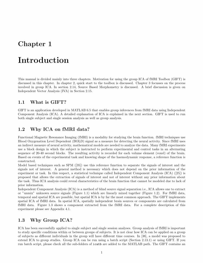
This manual is divided mainly into three chapters. Motivation for using the group ICA of fMRI Toolbox (GIFT) isdiscussed in this chapter. In chapter 2, quick start to the toolbox is discussed. Chapter 3 focusses on the processinvolved in group ICA. In section 2.14, Source Based Morphometry is discussed. A brief discussion is given onIndependent Vector Analysis (IVA) in Section 2.15.
1.1 What is GIFT?
GIFT is an application developed in MATLAB 6.5 that enables group inferences from fMRI data using IndependentComponent Analysis (ICA). A detailed explanation of ICA is explained in the next section. GIFT is used to runboth single subject and single session analysis as well as group analysis.
1.2 Why ICA on fMRI data?
Functional Magnetic Resonance Imaging (fMRI) is a modality for studying the brain function. fMRI techniques useBlood Oxygenation Level Dependent (BOLD) signal as a measure for detecting the neural activity. Since fMRI usesan indirect measure of neural activity, mathematical models are needed to analyze the data. Many fMRI experimentsuse a block design in which the subject is instructed to perform experimental and control tasks in an alternatingsequence of 20-40 second blocks. The resulting activity is recorded for each volume element (voxel) of the brain.Based on events of the experimental task and knowing shape of the haemodynamic response, a reference function isconstructed.Model based techniques such as SPM ([35]) use this reference function to separate the signals of interest and thesignals not of interest. A general method is necessary which does not depend on the prior information of theexperiment or task. In this respect, a statistical technique called Independent Component Analysis (ICA) ([25]) isproposed that allows the extraction of signals of interest and not of interest without any prior information aboutthe task. Thus ICA analysis could reveal characteristics of the brain function that cannot be modeled due to lack ofprior information.Independent Component Analysis (ICA) is a method of blind source signal separation i.e., ICA allows one to extractor ”unmix” unknown source signals (Figure 1.1) which are linearly mixed together (Figure 1.2). For fMRI data,temporal and spatial ICA are possible, but spatial ICA is by far the most common approach. The GIFT implementsspatial ICA of fMRI data. In spatial ICA, spatially independent brain sources or components are calculated fromfMRI data. Figure 1.3 shows a component extracted from the fMRI data. For a complete description of thisexperiment please see Appendix 4.1.
1.3 Why Group ICA?
ICA has been successfully applied to single subject and single session analyses. Group analysis of fMRI is importantto study specific conditions within or between groups of subjects. It is not clear how ICA can be applied on a groupof subjects as different individuals in the group will have different time courses. In [38], a model was proposed toextend ICA to group studies. Group ICA can be run using a batch script (Section 2.13.1) or using GIFT. If yourun batch script, please check all the sub-folders of icatb are added to the MATLAB path. The GIFT contains an
1

2 CHAPTER 1. INTRODUCTION
0 20 40 60 80 100 120 140−1
−0.5
0
0.5
1
0 20 40 60 80 100 120 1400
2
4
6
Figure 1.1: Unknown source signals.
0 20 40 60 80 100 120 1400
5
10
15
0 20 40 60 80 100 120 1400
2
4
6
Figure 1.2: Mixed signals.

1.3. WHY GROUP ICA? 3
0
9.2
−101
Scans
Component 4 Not Sorted
Figure 1.3: A component consists of a time course and a spatial map.
implementation of ICA for analyzing the fMRI data. Specifically, the GIFT implements both analysis and displaytools, each using standard input and output file types (Analyze or Nifti format). There are three main stages toGroup ICA; Data Compression, ICA, and Back Reconstruction ([38]). The outputs from these stages are multipletime courses. Each time course has an image map associated with it. A detailed explanation of the process involvedin group ICA is discussed in the Chapter 3.

4 CHAPTER 1. INTRODUCTION

Chapter 2
Getting Started with GIFT
The source code and the example subjects fMRI data need to be installed. These are available on project web page:
http://icatb.sourceforge.net
Also available on this web page are posters on GIFT at the conferences like Society of Biological Psychiatry andHuman Brain Mapping. The mailing list is:
Please send comments and bug reports to:
[email protected] or [email protected]
2.1 Installing GIFT
Unzip the file GroupICATv3.0a.zip and copy the folder GroupICATv3.0a onto your local machine. Add GIFT direc-tories to the MATLAB search path or run the gift.m file to automatically add GIFT directories. The GIFT pathby default will be set at the bottom of the MATLAB path. You can create gift_startup.m (Appendix 4.7) file forsetting the path according to your needs. After the GIFT path is set, GIFT toolbox (Figure 2.1) opens in a newfigure window. There is also an option to run group ICA using a batch script (Section 2.13.1). Batch script is veryuseful for running large data-sets.
Note:
• GIFT toolbox can also be invoked by using the statement groupica and clicking on the fMRI button or bytyping groupica fmri at the MATLAB command window.
• If you have downloaded an older version of GIFT, make sure that there is only one version on path at a time.
2.2 Installing Example Subjects
Download the example_subjects.zip file and unzip into an appropriate directory. Included in this file are threesubjects pre-processed fMRI data from a visuomotor task (See [38] for a complete description of the task). Wholebrain and single slice data (for rapid testing) are provided. More information on the task the subject performedwhile in the scanner is given in the Appendix 4.1. Each example subject also contains a functional data-set, whichcontains only one brain slice. If you are having problems with this toolbox you may test this with a smaller data-set.
2.3 HTML Help
When you click Help button (Figure 2.1), HTML help manual is opened in the default web browser. ”GIFT-help”menu is plotted on some figures which will directly open a particular topic.
5

6 CHAPTER 2. GETTING STARTED WITH GIFT
2.4 Changes from the release GroupICATv2.0e
• A new dynamic functional network connectivity (dFNC) toolbox is integrated within the GIFT toolbox. Pleasesee Section 2.12.4 to use the toolbox.
• A new algorithm for independent vector analysis (IVA-GL) is integrated into the GIFT toolbox. IVA-GL usesmulti-variate gaussian prior and laplacian prior to do source separation from the data. Please see Section 2.15for more information.
• Multivariate Objective Optimization ICA with Reference (MOO-ICAR) is now integrated in the GIFT toolbox.MOO-ICAR uses a no data reduction approach and aggregate component maps from previous group ICAanalysis as reference to estimate sources of interest for each subject. Please see [40] for more information.
• Constrained ICA (Spatial) approach is updated to allow for the no data reduction approach similar to MOO-ICAR method above.
• PCA using eigen decomposition method is modified to compute the covariance matrix along the smallestdimension of the data.
• Statistics tool to compute T-test, ANOVA and Multiple Regression on subject ICA loading coefficients havenow been added to the SBM toolbox.
Note: Dependencies on Statistical, Image Processing and Signal Processing MATLAB toolboxes are removedwhen using MANCOVAN toolbox.
2.5 GIFT Updates
We post the updates to the software that contain new features or any bug fixes in the updates section of the projectweb page. Please see Updates_Readme.txt for more details.
2.6 Things to do before configuring the analysis
2.6.1 Compiling MEX files
• SPM MEX binaries - We use SPM8 volume functions to read and write image data.
• Group ICA MEX binaries - C-MEX files are provided for computing the eigen values of a symmetric matrix.The compiled MEX binaries are used only when you select packed storage scheme for computing covariancematrix during the second or third data reduction stage.
• GLASSO - FORTRAN MEX file ([6]) is provided for estimating a sparse inverse covariance matrix using a L1penalty when using dFNC toolbox.
To compile the MEX source code, type icatb_compile_mex_files at the MATLAB command prompt. Please seebelow to copy the SPM MEX binaries manually if the source code fails to compile:
• Copy SPM8 MEX binaries like spm_bwlabel*, spm_existfile*, spm_sample_vol*, spm_slice_vol* to thedirectory icatb\icatb_spm8_files and prefix them with icatb_.
• Copy SPM8MEX binaries like spm8\@file_array\private\* to icatb_spm8_files\@icatb_file_array\privateand prefix them with icatb_.
Note: * refers to the MEX file extension on your Operating System. Type mexext on the MATLAB commandwindow to get the MEX file extension on the Operating System you are working on.
2.6.2 Memory Requirements
Since PCA and ICA are Multi-variate approaches unlike General Linear Model, there are some memory requirementsto do the group ICA/IVA analysis. We added a script icatb_mem_ica.m which will give a close estimate of RAMrequired to do the group ICA/IVA analysis. Please enter the parameters like number of voxels, time points, subjects,sessions, components and reduction steps in the input parameters section of the script and run the script to get anapproximate amount of RAM required.
2.6. THINGS TO DO BEFORE CONFIGURING THE ANALYSIS 7
2.6.3 Organizing Data
Organizing data reduces the amount of selection. GIFT has two ways to enter the data for GUI and four ways toenter the data using the batch script.
• First method requires the data to be in one root folder with a common file pattern (like sw*.img) for allsubjects and sessions. Each subject folder can have session folders and the number of session folders with thematching file pattern should be the same over subjects.
• Second method does not require the data to be in one root folder or have a common file pattern but theselection process through GUI can be tedious for large data-sets and therefore batch script (Section 2.13.1)isrecommended.
• Third method uses regular expressions to get the subject and session directories. This option is useful inmatching directories that have nested paths. However, this option still requires a common file pattern for allthe subjects. Please see Section 2.13.1 for more information.
• Option is provided to paste the file names in the fourth method (Section 2.13.1).
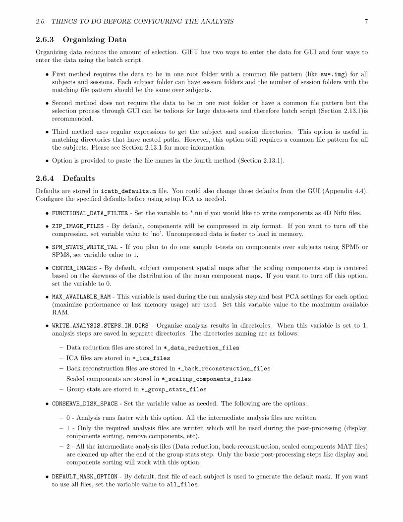
2.6.4 Defaults
Defaults are stored in icatb_defaults.m file. You could also change these defaults from the GUI (Appendix 4.4).Configure the specified defaults before using setup ICA as needed.
• FUNCTIONAL_DATA_FILTER - Set the variable to *.nii if you would like to write components as 4D Nifti files.
• ZIP_IMAGE_FILES - By default, components will be compressed in zip format. If you want to turn off thecompression, set variable value to ’no’. Uncompressed data is faster to load in memory.
• SPM_STATS_WRITE_TAL - If you plan to do one sample t-tests on components over subjects using SPM5 orSPM8, set variable value to 1.
• CENTER_IMAGES - By default, subject component spatial maps after the scaling components step is centeredbased on the skewness of the distribution of the mean component maps. If you want to turn off this option,set the variable to 0.
• MAX_AVAILABLE_RAM - This variable is used during the run analysis step and best PCA settings for each option(maximize performance or less memory usage) are used. Set this variable value to the maximum availableRAM.
• WRITE_ANALYSIS_STEPS_IN_DIRS - Organize analysis results in directories. When this variable is set to 1,analysis steps are saved in separate directories. The directories naming are as follows:
– Data reduction files are stored in *_data_reduction_files
– ICA files are stored in *_ica_files
– Back-reconstruction files are stored in *_back_reconstruction_files
– Scaled components are stored in *_scaling_components_files
– Group stats are stored in *_group_stats_files
• CONSERVE_DISK_SPACE - Set the variable value as needed. The following are the options:
– 0 - Analysis runs faster with this option. All the intermediate analysis files are written.
– 1 - Only the required analysis files are written which will be used during the post-processing (display,components sorting, remove components, etc).
– 2 - All the intermediate analysis files (Data reduction, back-reconstruction, scaled components MAT files)are cleaned up after the end of the group stats step. Only the basic post-processing steps like display andcomponents sorting will work with this option.
• DEFAULT_MASK_OPTION - By default, first file of each subject is used to generate the default mask. If you wantto use all files, set the variable value to all_files.
8 CHAPTER 2. GETTING STARTED WITH GIFT
• REMOVE_CONSTANT_VOXELS - Constant voxels are removed in the fMRI data when this variable is set to 1.
• DEFAULT_MASK_SBM_MULTIPLIER - Default mask multiplier in SBM. Defaults is 1% of mean i.e., voxels greaterthan or equal to 1% of mean will be used.
2.7 Spatial Templates
The following example spatial templates are provided in icatb\icatb_templates:
• ref_right_visuomotor.nii - Mask containing the right visual regions.
• ref_left_visuomotor.nii - Mask containing the left visual regions.
• ref_default_mode.nii - Mask containing the default mode network regions. Please see [5] for more informa-tion.
• *DMN_ICA_REST*.nii - This mask was created from a data-set of 42 subjects. During a fMRI scan, subjects wereasked to relax and passively stare at a fixation cross. A pooled group ICA was performed and the default modecomponent network was selected to create this mask. We provide templates like rDMN_ICA_REST_3x3x3.nii
and rDMN_ICA_REST_3x3x4.nii in the GIFT. Please see [4] for more information.
• *DMN_MASK.WFU*.nii - This mask was constructed using the Wake Forest Pick atlas toolbox. A binary maskwas created by selecting the anatomical regions that have been most commonly reported to comprise thedefault mode network. The labels from the Wake Forest Atlas that constituted this mask included poste-rior cingulate (BAs 23/31), inferior and superior parietal lobes (BAs 7/39/40), superior frontal gyrus (BAs8/9/10), and anterior cingulate cortex (BAs 11/32). In addition, a larger weight was given to the anterior andposterior cingulate cortex, which are believed to be the central nodes of the default mode network. A highercorrelation was observed when giving a higher weight to these two central nodes. We provide templates likerDMN_MASK.WFU.3x3x3.nii and rDMN_MASK.WFU.3x3x4.nii in the GIFT. Please see [4] for more information.
2.8 Menus
Menus are provided as a shortcut to the user-interface controls in the GIFT toolbox (Figure 2.1). The function ofeach menu is given below:
• File
– New - Setup ICA GUI will open after you have selected the output directory.
– Open - Setup ICA GUI will open showing the values for the parameters after you have selected the subjectfile that has suffix Subject.mat.
– Close - Closes the GIFT Toolbox and the figures generated by the GIFT.
• View
– Analysis Info - Analysis information will be shown after you have selected the parameter file that hassuffix ica_parameter_info.mat.
• Tools
– Run Analysis - Analysis will be run after you have selected the parameter file.
– Display GUI - Display GUI will be opened after you have selected the parameter file.
– Utilities
∗ Batch - Option is now provided to select the input files for batch analysis. More information on inputfile is provided in Section 2.13.1.
∗ Remove Component(s) - Removes a component or components from the data after you have selectedthe parameter file. Please see section 2.12.1 for more information.

2.9. ANALYSIS FUNCTIONS 9
∗ Mancovan - Mancovan toolbox works on the ICA output. Multi variate stats is used to determinethe significant covariates which will be used later in the univariate tests. Please see 2.12.3 for moreinformation.
∗ dFNC - Dynamic FNC (dFNC) toolbox is used to study functional network connectivity dynamics.dFNC toolbox is based on paper [13]. Please see 2.12.4 for using the toolbox.
∗ Component viewer - Orthogonal views of the selected component and its power spectra are displayed.
∗ ICASSO - ICASSO plugin is used to assess the stability of components. Please see Section 2.12.2 formore information.
∗ Ascii_to_spm.mat - Creates SPM.mat from ascii file (containing regressor time courses) that is neededduring temporal sorting. Please see Section 2.12.5 for more information.
∗ Event Average - Event average is calculated for the ICA time courses. Please see Section 2.12.6 formore information.
∗ Calculate Stats - Mean, standard deviation, t-maps are calculated for components over sessions,subjects or subjects and sessions.
∗ Spectral Group Compare - This utility is used to compare the power spectra between groups. Pleasesee Section 2.12.8 for more information.
∗ Stats On Beta Weights - This utility is provided for doing statistics on the time courses (beta weights).Please see Section 2.12.9 for running this utility.
∗ SPM Stats - This utility is used to do one sample t-test or two sample t-test on the component images.Please see Section 2.13.1 for more information.
∗ Spatial-temporal regression - Given a set of GLM or ICA spatial maps and the original data of thesubjects, you could use this utility to back reconstruct subject components (Section 2.12.12).
∗ Write Talairach Table - Talairach daemon client is used to generate the talairach tables for the selectedimage. Please see Section 2.12.11 for more information.
∗ Single Trial Amplitudes - We provide the option for calculating single trial amplitudes (Section 2.12.13)in GIFT.
∗ Z-shift - Please see Section 2.12.14 for more information.
∗ Percent Variance - This utility can be used after running the group ICA analysis. Please see Section2.12.15 for more information.
2.9 Analysis Functions
2.9.1 Setup ICA Analysis
When you click Setup ICA button (Figure 2.1), Setup ICA GUI (Figure 2.2) will open after you have selected theoutput directory for the analysis. Setup ICA is the GUI used for entering parameters required for group ICA. Figure2.2 shows the main user interface controls. Some of the parameters are plotted in ”Setup ICA-Defaults” menu (Figure2.3). It is recommended that after entering the parameters in the main figure window parameters plotted in menube changed. The parameters are explained below:
Main User Interface Controls
• ’Enter Name (Prefix) Of Output Files’ is the prefix string to all the output files created by GIFT. This shouldbe a valid character name as the files will be saved using this prefix.
Note: Avoid characters like \, /, :, *, ?, ”, < and > in the prefix.
• ’Have You Selected the fMRI Data Files?’ Click on the push button Select to select the data. There are twooptions for selecting the data as explained in Section 2.6.3. After the data is selected, the push button Selectwill be changed to popup with ’Yes’ and ’No’ as the options.
– ’Yes’ - Data reduction steps will be enabled if you have selected the parameters previously with the sameoutput prefix.
– ’No’ - the data can be selected again.
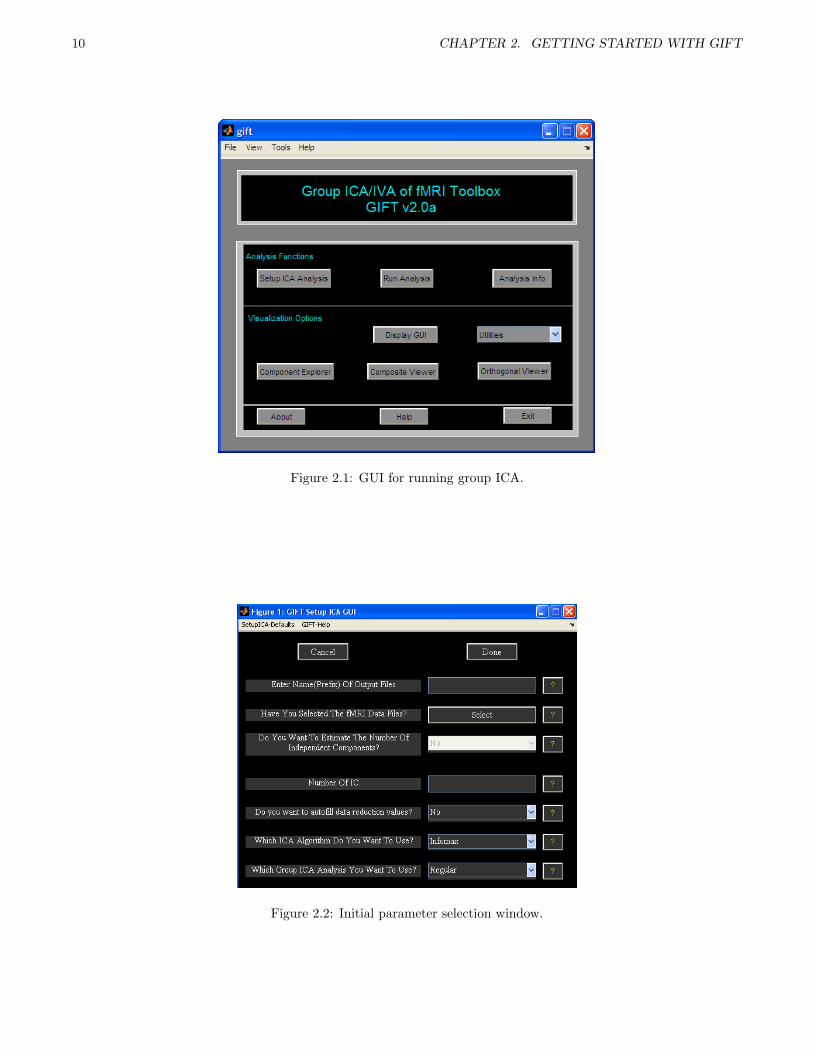
10 CHAPTER 2. GETTING STARTED WITH GIFT
Figure 2.1: GUI for running group ICA.
Figure 2.2: Initial parameter selection window.

2.9. ANALYSIS FUNCTIONS 11
Figure 2.3: Hidden user interface controls.
Figure 2.4: PCA Options.

12 CHAPTER 2. GETTING STARTED WITH GIFT
Note: After the data-sets are selected, a file will be saved with suffix Subject.mat. This MAT file containsinformation about number of subjects, sessions and files.
• ’Do you want to estimate the number of independent components?’ Components are estimated ([41]) fromthe fMRI data using the MDL criteria. All the data-sets or a particular data-set can be used to estimate thecomponents. When all the data-sets are used estimated components are calculated by using the mean of theestimated components of all data-sets.
• ’Number of IC’ refers to the number of independent components that will be extracted from the data.
Note: If you have selected Constrained ICA (Spatial) algorithm, the number of independent componentsis set to the number of spatial reference files selected.
• ’Do you want to auto fill data reduction values?’ By default this option is set to ’Yes’ when the data is selectedand the ’Number of IC’ is set to 20. If there are more than one data reduction step, initial PC numbers areset to 1.5 times the number of final components.
• ’Which Algorithm Do You Want To Use?’ There are 16 ICA/IVA algorithms available like Infomax, FastICA,ERICA, SIMBEC, EVD, JADE OPAC, AMUSE, SDD ICA, Semi-blind Infomax, Constrained ICA (Spatial),Radical ICA, Combi, ICA-EBM, FBSS, IVA-GL and MOO-ICAR.
• ’Which Group ICA Analysis You Want To Use?’ Options are ’Regular’ and ’ICASSO’. When you select’ICASSO’, ICA is run several times and the best estimate for each component is used (See Section 2.12.2).Please note that algorithms like JADE OPAC, Constrained ICA (Spatial), MOO-ICAR and IVA-GL don’twork with ICASSO.
Note: If the auto fill data reduction steps drop down box is set to ’No’ after entering the prefix, check the numbersfor principal components by clicking the ”Setup-ICA Defaults” menu. (Figure 2.3).
Hidden User Interface Controls
• ’Select Type Of Data Pre-processing’ - Data is pre-processed prior to the first data reduction. Options arediscussed below.
– ’Remove Mean Per Timepoint’ - At each time point, image mean is removed.
– ’Remove Mean Per Voxel’ - Time-series mean is removed at each voxel.
– ’Intensity Normalization’ - At each voxel, time-series is scaled to have a mean of 100. When intensitynormalization is selected as the pre-processing step, don’t use z-scores or percent signal change for scalingcomponents.
– ’Variance Normalization’ - At each voxel, time-series is linearly detrended and converted to z-scores.
• ’What Mask Do You Want To Use?’ There are two options like ’Default Mask’ and ’Select Mask’.
– ’Default Mask’ - Mask is calculated using all the files for subjects and sessions or only the first file foreach subject and session depending upon the variable DEFAULT_MASK_OPTION value in defaults. BooleanAND operation is done to include the voxels that surpass the mean of each subject’s session.
Note: By default first file for each subject session is selected because using all the files is time consuming.You can use all the files for each subject and session by setting variable DEFAULT_MASK_OPTION value toall_files.
– ’Select Mask’ - You can specify a mask containing the selected regions for the analysis. This mask mustbe in Analyze or Nifti format.
• ’Select Type Of PCA’ - There are three options like ’Standard’, ’Expectation Maximization’ and ’SVD’. PCAoptions window (Figure 2.4) will change depending on the type of PCA selected.
– Standard
∗ ’Do You Want To Stack Datasets?’ - Options are ’Yes’ and ’No’.

2.9. ANALYSIS FUNCTIONS 13
· ’Yes’ - Data sets are stacked to compute covariance matrix. This option assumes that there isenough RAM available to stack the data sets and for computing covariance matrix. Please notethat full storage of covariance matrix is required when you select this option.
· ’No’ - A pair of data sets are loaded at a time to compute covariance matrix. This option usesless memory but it requires NC2 loops to compute the covariance matrix where N is the numberof data sets.
∗ ’Select Matrix Storage Type’ - Options are ’Full’ and ’Packed’. You have the option to store onlylower triangular portion of the symmetric matrix with the packed storage scheme.
∗ ’Select Precision’ - Options are ’Double’ and ’Single’. Single precision uses 50% less memory requiredwhen compared to double precision. Single precision is accurate up to 7 digits after decimal point.
∗ ’Select Eigen Solver Type’ - Options are ’Selective’ and ’All’. These options will be used only for thepacked storage scheme.
· ’Selective’ - Only a few desired eigen values are computed. This option will compute eigen valuesfaster when compared to ’All’ option. However, if there are convergence issues use option ’All’ tocompute eigen values.
· ’All’ - All eigen values are computed. We recommend to use this option for computing eigenvalues only when the selective eigen solver doesn’t converge.
– Expectation Maximization (EM PCA) has fewer memory constraints and is advantageous over standardPCA when only few eigen values need to be computed from a large data-set ([34]). PCA options of thisapproach are discussed below:
∗ ’Do You Want To Stack Datasets?’ - Options are ’Yes’ and ’No’.
· ’Yes’ - This option assumes that there is enough RAM available to stack the data sets.
· ’No’ - A data-set is loaded at a time to compute transformation matrix at each iteration. Thisoption may take days to solve the problem if there are very large data-sets.
∗ ’Select Precision’ - Options are ’Double’ and ’Single’.
∗ ’Select Stopping Tolerance’ - Norm of residual error is used. Residual error is computed by subtractingthe transformation matrix at the current iteration from the previous iteration.
∗ ’Enter Max No. Of Iterations’ - Maximum number of iterations to use.
– SVD - Singular value decomposition (SVD) is preferable when the data is ill-conditioned. Memory re-quirements of SVD are similar to covariance based PCA.
∗ ’Select Precision’ - Options are ’Double’ and ’Single’.
∗ ’Select Solver’ - Options are ’Selective’ and ’All’.
Note:
∗ Before setting up analysis, please see icatb_mem_ica.m script to get a close estimate of the RAMrequired for all the analysis types. In general for better performance, stack data-sets using singleprecision. However, if memory is an issue don’t stack data-sets and use slower ways to compute PCA(EM PCA or packed storage scheme of standard PCA).
∗ By default, GIFT will save MAT files in the uncompressed format (-v6). Always use uncompressedformat if you want a better performance during the analysis phase.
• ’Select The Type Of Group PCA’ - Options are ’subject specific’ and ’grand mean’.
– ’Subject Specific’ - PCA is done on each data-set before doing group PCA.
– ’Grand Mean’ - Each data-set is projected on to the eigen space of the mean of all data-sets before doinggroup PCA ([26]). This PCA requires that time points or images are the same between the data-sets.
Note:
– Subject specific approach retains maximum variance at the individual level PCA when compared to thegrand mean approach.
– Grand mean approach retains more variance at the group PCA when compared to the subject specificapproach.
14 CHAPTER 2. GETTING STARTED WITH GIFT
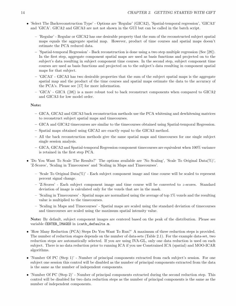
• ’Select The Backreconstruction Type’ - Options are ’Regular’ (GICA2), ’Spatial-temporal regression’, ’GICA3’and ’GICA’. GICA2 and GICA3 are not not shown in the GUI but can be called in the batch script.
– ’Regular’ - Regular or GICA2 has one desirable property that the sum of the reconstructed subject spatialmaps equals the aggregate spatial map. However, product of time courses and spatial maps doesn’testimate the PCA reduced data.
– ’Spatial-temporal Regression’ - Back reconstruction is done using a two step multiple regression (See [28]).In the first step, aggregate component spatial maps are used as basis functions and projected on to thesubject’s data resulting in subject component time courses. In the second step, subject component timecourses are used as basis functions and projected on to the subject’s data resulting in component spatialmaps for that subject.
– ’GICA3’ - GICA3 has two desirable properties that the sum of the subject spatial maps is the aggregatespatial map and the product of the time courses and spatial maps estimate the data to the accuracy ofthe PCA’s. Please see [17] for more information.
– ’GICA’ - GICA ([38]) is a more robust tool to back reconstruct components when compared to GICA2and GICA3 for low model order.
Note:
– GICA, GICA2 and GICA3 back reconstruction methods use the PCA whitening and dewhitening matricesto reconstruct subject spatial maps and timecourses.
– GICA and GICA2 timecourses are similar to the timecourses obtained using Spatial-temporal Regression.
– Spatial maps obtained using GICA2 are exactly equal to the GICA3 method.
– All the back reconstruction methods give the same spatial maps and timecourses for one single subjectsingle session analysis.
– GICA, GICA2 and Spatial-temporal Regression component timecourses are equivalent when 100% varianceis retained in the first step PCA.
• ’Do You Want To Scale The Results?’ The options available are ’No Scaling’, ’Scale To Original Data(%)’,’Z-Scores’, ’Scaling in Timecourses’ and ’Scaling in Maps and Timecourses’.
– ’Scale To Original Data(%)’ - Each subject component image and time course will be scaled to representpercent signal change.
– ’Z-Scores’ - Each subject component image and time course will be converted to z-scores. Standarddeviation of image is calculated only for the voxels that are in the mask.
– ’Scaling in Timecourses’ - Spatial maps are normalized using the average of top 1% voxels and the resultingvalue is multiplied to the timecourses.
– ’Scaling in Maps and Timecourses’ - Spatial maps are scaled using the standard deviation of timecoursesand timecourses are scaled using the maximum spatial intensity value.
Note: By default, subject component images are centered based on the peak of the distribution. Please seevariable CENTER_IMAGES in icatb_defaults.m.
• ’How Many Reduction (PCA) Steps Do You Want To Run?’ A maximum of three reduction steps is provided.The number of reduction stages depends on the number of data-sets (Table 2.1). For the example data-set, tworeduction steps are automatically selected. If you are using IVA-GL, only one data reduction is used on eachsubject. There is no data reduction prior to running ICA if you use Constrained ICA (spatial) and MOO-ICARalgorithms.
• ’Number Of PC (Step 1)’ - Number of principal components extracted from each subject’s session. For onesubject one session this control will be disabled as the number of principal components extracted from the datais the same as the number of independent components.
• ’Number Of PC (Step 2)’ - Number of principal components extracted during the second reduction step. Thiscontrol will be disabled for two data reduction steps as the number of principal components is the same as thenumber of independent components.
2.9. ANALYSIS FUNCTIONS 15
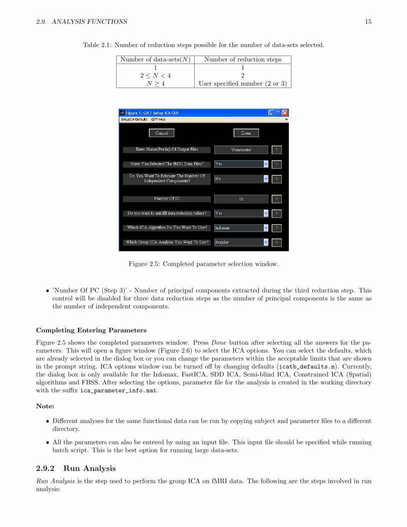
Table 2.1: Number of reduction steps possible for the number of data-sets selected.
Number of data-sets(N) Number of reduction steps1 1
2 ≤ N < 4 2N ≥ 4 User specified number (2 or 3)
Figure 2.5: Completed parameter selection window.
• ’Number Of PC (Step 3)’ - Number of principal components extracted during the third reduction step. Thiscontrol will be disabled for three data reduction steps as the number of principal components is the same asthe number of independent components.
Completing Entering Parameters
Figure 2.5 shows the completed parameters window. Press Done button after selecting all the answers for the pa-rameters. This will open a figure window (Figure 2.6) to select the ICA options. You can select the defaults, whichare already selected in the dialog box or you can change the parameters within the acceptable limits that are shownin the prompt string. ICA options window can be turned off by changing defaults (icatb_defaults.m). Currently,the dialog box is only available for the Infomax, FastICA, SDD ICA, Semi-blind ICA, Constrained ICA (Spatial)algorithms and FBSS. After selecting the options, parameter file for the analysis is created in the working directorywith the suffix ica_parameter_info.mat.
Note:
• Different analyses for the same functional data can be run by copying subject and parameter files to a differentdirectory.
• All the parameters can also be entered by using an input file. This input file should be specified while runningbatch script. This is the best option for running large data-sets.
2.9.2 Run Analysis
Run Analysis is the step used to perform the group ICA on fMRI data. The following are the steps involved in runanalysis:

16 CHAPTER 2. GETTING STARTED WITH GIFT
Figure 2.6: ICA Options Window
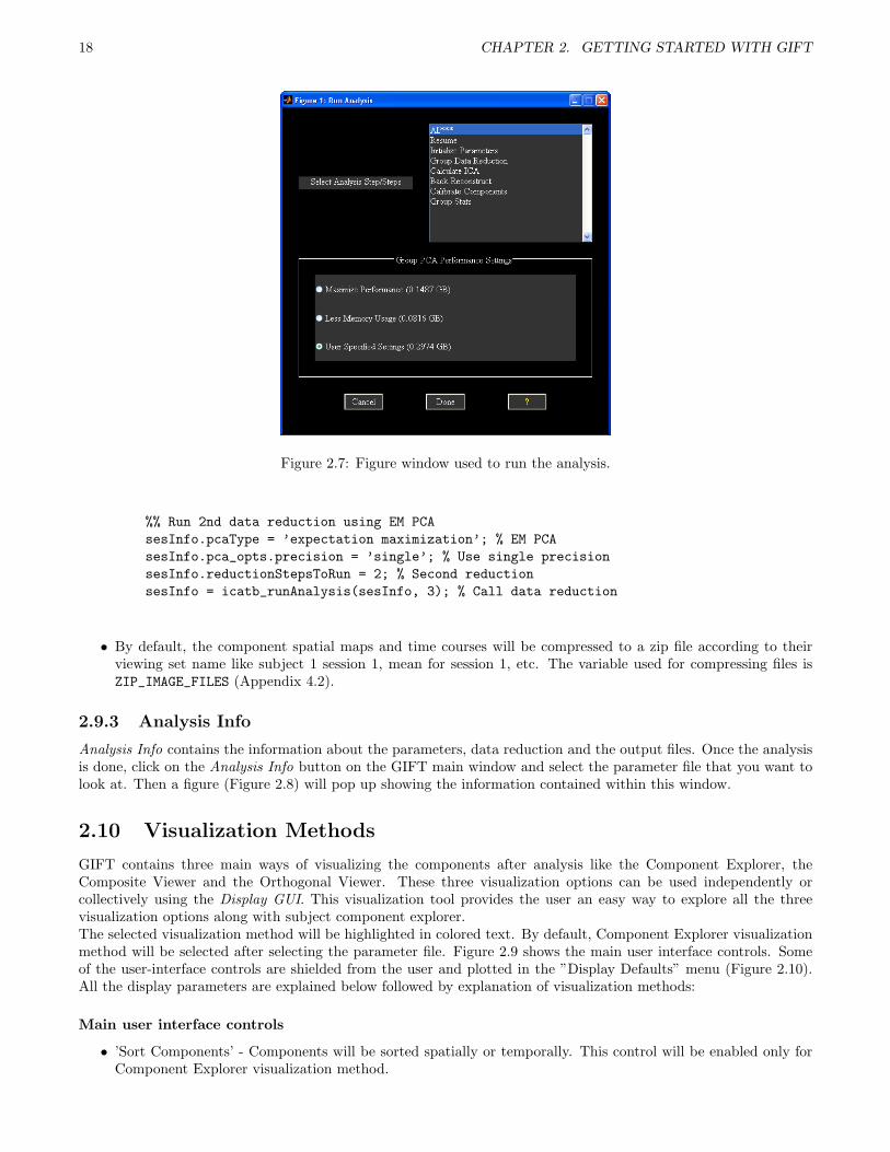
• The parameter file required for the analysis should be selected. This file is the same file where you enteredall the analysis information. It is named as ica_parameter_info.mat. Once the parameter file is selected, afigure (Figure 2.7) will pop up showing the options for run analysis. The options are as follows:
– ’All***’
∗ All the group ICA steps are run at once. The analysis can also be run by selecting steps from’Parameter Initialization’ to ’Group Stats’ in order.
– ’Resume’
∗ Resume option used to handle interrupted analysis. Resume option also detects changes in the userinput and runs the appropriate group ICA steps. For example, if you changed back-reconstructionapproach resume option runs the steps from back-reconstruction to group stats.
– ’Parameter Initialization’
∗ All the variables that are needed later on or during the analysis are declared and initialized.
∗ A parameter error check is also preformed to try and catch errors before the group analysis begins.
– ’Data Reduction’
∗ Each data-set is reduced using Principle Components Analysis (PCA). These reduced data-sets arethen concatenated into a group or groups depending on the number of data reductions steps selected,this process is repeated.
∗ Each reduced data is saved in a MAT file and will be used in the back reconstruction step.
– ’Calculate ICA’
∗ The concatenated data from the data reduction step is used and the aggregate ICA components aresaved in both MAT and Analyze (or Nifti) format.
– ’Back Reconstruction’
∗ · For ’GICA’, ’GICA2’ and ’GICA3’, the aggregate components and the results from data reductionare used to compute the individual subject components.
· ’Spatial-temporal Regression’ - The aggregate components and the original data are used to com-pute the individual subject components.

2.9. ANALYSIS FUNCTIONS 17
∗ The individual subject components are saved in Analyze (or Nifti) format.
– ’Calibrating Components’
∗ By default, components are in arbitrary units. Components are scaled to percent signal change,z-scores, scaling in timecourses or scaling in maps and timecourses.
– ’Group Stats’
∗ The individual back reconstructed components are used to compute a mean spatial map and timecourse, a standard deviation spatial map and time course and a t-statistic spatial map. The timecourse used for the t-statistic component is the mean time course. These group stats components arecalculated for each session and are saved in Analyze (or Nifti) format.
∗ Results during each of the steps are printed to the MATLAB command window. After the analysisis completed, Display GUI (Figure 2.9) will open automatically for visualizing components.
• Group PCA Performance Settings - There are three options like ’Maximize Performance’, ’Less Memory Usage’and ’User Specified Settings’. Best match for each option is selected based on the variable MAX_AVAILABLE_RAM.PCA types selected will be between covariance based and expectation maximization approaches.
– ’Maximize Performance’ - Reduced data-sets from the first data reduction step are stacked by default.
– ’Less Memory Usage’ - Slower ways of computing PCA are used.
– ’User Specified Settings’ - User specified PCA options are selected.
Note:
• All the analysis information is stored in the _results.log file. This file gets appended each time the analysisis run with the same prefix for the output files.
• Run analysis steps can also be accessed from the command line.
load(param_file); % Load parameter file (*ica*param*mat)
sesInfo = icatb_runAnalysis(sesInfo, 1); % Run All Steps
sesInfo = icatb_runAnalysis(sesInfo, 2); % Parameter Initialization
sesInfo = icatb_runAnalysis(sesInfo, 3); % Data Reduction
sesInfo = icatb_runAnalysis(sesInfo, 4); % ICA
sesInfo = icatb_runAnalysis(sesInfo, 5); % Back reconstruction
sesInfo = icatb_runAnalysis(sesInfo, 6); % Scaling components
sesInfo = icatb_runAnalysis(sesInfo, 7); % Group Stats
sesInfo = icatb_runAnalysis(sesInfo, 8); % Resume interrupted analysis
• Option is provided in the GIFT to run a particular data reduction step. This is useful when a particular datareduction step was already done and you would like to go to the next step without re-running the earlier step.
load(param_file); % Load parameter file (*ica*param*mat)
sesInfo.reductionStepsToRun = 2; %Run 2nd reduction only
sesInfo = icatb_runAnalysis(sesInfo, 3); % Call Data Reduction
• You could also switch between PCA types using command line. For example, the first data reduction could bedone using Standard PCA and the memory intensive second data reduction could be done using ExpectationMaximization.
load(param_file); % Load parameter file (*ica*param*mat)
%% Run 1st data reduction using Standard PCA
sesInfo.pcaType = ’standard’; % Standard PCA
sesInfo.reductionStepsToRun = 1; % First reduction
sesInfo = icatb_runAnalysis(sesInfo, 3); % Call data reduction
18 CHAPTER 2. GETTING STARTED WITH GIFT
Figure 2.7: Figure window used to run the analysis.
%% Run 2nd data reduction using EM PCA
sesInfo.pcaType = ’expectation maximization’; % EM PCA
sesInfo.pca_opts.precision = ’single’; % Use single precision
sesInfo.reductionStepsToRun = 2; % Second reduction
sesInfo = icatb_runAnalysis(sesInfo, 3); % Call data reduction
• By default, the component spatial maps and time courses will be compressed to a zip file according to theirviewing set name like subject 1 session 1, mean for session 1, etc. The variable used for compressing files isZIP_IMAGE_FILES (Appendix 4.2).
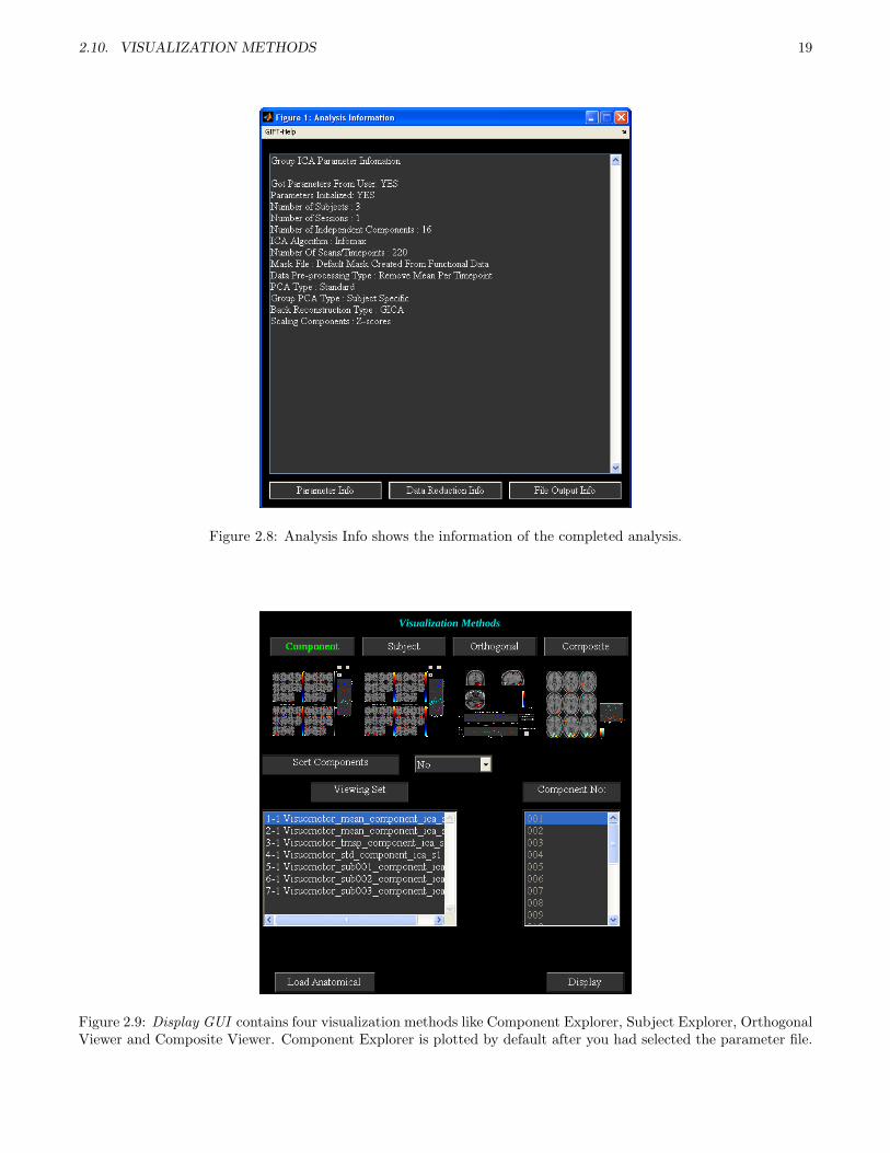
2.9.3 Analysis Info
Analysis Info contains the information about the parameters, data reduction and the output files. Once the analysisis done, click on the Analysis Info button on the GIFT main window and select the parameter file that you want tolook at. Then a figure (Figure 2.8) will pop up showing the information contained within this window.
2.10 Visualization Methods
GIFT contains three main ways of visualizing the components after analysis like the Component Explorer, theComposite Viewer and the Orthogonal Viewer. These three visualization options can be used independently orcollectively using the Display GUI. This visualization tool provides the user an easy way to explore all the threevisualization options along with subject component explorer.The selected visualization method will be highlighted in colored text. By default, Component Explorer visualizationmethod will be selected after selecting the parameter file. Figure 2.9 shows the main user interface controls. Someof the user-interface controls are shielded from the user and plotted in the ”Display Defaults” menu (Figure 2.10).All the display parameters are explained below followed by explanation of visualization methods:
Main user interface controls
• ’Sort Components’ - Components will be sorted spatially or temporally. This control will be enabled only forComponent Explorer visualization method.
2.10. VISUALIZATION METHODS 19
Figure 2.8: Analysis Info shows the information of the completed analysis.
Visualization Methods
Figure 2.9: Display GUI contains four visualization methods like Component Explorer, Subject Explorer, OrthogonalViewer and Composite Viewer. Component Explorer is plotted by default after you had selected the parameter file.

20 CHAPTER 2. GETTING STARTED WITH GIFT
Figure 2.10: User interface controls plotted in ”Display Defaults” menu
• ’Viewing Set’ - This is the component viewing set to look at like subject 1 session 1, mean for session 1, etcand will be disabled for Subject Explorer visualization method.
• ’Component number’ - Component number/numbers to look at. This will be disabled for Component Explorervisualization method.
• Load Anatomical - Load Anatomical button is used to select anatomical image. Component images will beoverlaid on this anatomical image. By default, first image of functional data will be used as an anatomicalimage.
• Display - Display button is used to display the components of different visualization methods.
• Display Defaults menu - Hidden display parameters will be shown in a figure (Figure 2.10) when you click onDisplay Defaults menu. This figure contains parameters like ’Image Values’, ’Anatomical Plane’, ’Threshold’,’Slice Range’ and ’Images Per Figure’. ”Display GUI Options” menu can be used to change design matrix andselecting the text file (See Appendix 4.2) that contains regressor information for temporal sorting. Select ’DesignMatrix’ for selecting design matrix for temporal sorting. There are three options for selecting design matrixlike ’Same regressors for all subjects and sessions’, ’Different regressors over sessions’, ’Different regressors forsubjects and sessions’. The options are explained below:
– ’Same regressors for all subjects and sessions’ - The regressors used will be the same over data-sets. Thiswill open a figure window for selecting SPM design matrix.
– ’Different regressors over sessions’ - The regressors used will be the same over subjects but different oversessions. This will open a figure window for selecting SPM design matrix.
– ’Different regressors over subjects and sessions’ - Different regressors can be used for each subject’s session.This will open a figure window for selecting a design matrix for each subject.
User Controls in Display Defaults menu
• ’Image Values’ - There are four options like ’Positive’, ’Positive and Negative’, ’Absolute’, ’Negative’. ’Positive’and ’Negative’ refer to activations and de-activations on spatial map. You should also look at the time course(flipped or un-flipped) to make the conclusion.
• ’Convert To Z-scores’ - Converts spatial maps to z-scores.
• ’Threshold Value’ - This is the z threshold value.
• ’Images Per Figure’ - Number of images per figure for Component Explorer and Subject Explorer visualizationmethods.
• ’Anatomical Plane’ - This is the anatomical plane to look at for Component Explorer, Subject Explorer andComposite Viewer.

2.10. VISUALIZATION METHODS 21
80 76 72 68 64 60 56
52 48 44 40 36 32 28
24 20 16 12 8 4 0
−4 −8 −12 −16 −20 −24 −28
−32 −36 −40 −44 −48 −52
LR
0
18.2
−2
0
2
Scans
Component 1 Not Sorted
80 76 72 68 64 60 56
52 48 44 40 36 32 28
24 20 16 12 8 4 0
−4 −8 −12 −16 −20 −24 −28
−32 −36 −40 −44 −48 −52
LR
0
10
−101
Scans
Component 2 Not Sorted
80 76 72 68 64 60 56
52 48 44 40 36 32 28
24 20 16 12 8 4 0
−4 −8 −12 −16 −20 −24 −28
−32 −36 −40 −44 −48 −52
LR
0
5.9
−0.200.20.4
Scans
Component 3 Not Sorted
80 76 72 68 64 60 56
52 48 44 40 36 32 28
24 20 16 12 8 4 0
−4 −8 −12 −16 −20 −24 −28
−32 −36 −40 −44 −48 −52
LR
0
5.6
−0.500.5
Scans
Component 4 Not Sorted
Figure 2.11: Figure shows the components not sorted in groupings of four.
• ’Slices Range’ - Slices plotted in mm. Slices in mm are calculated based on the anatomical data. You canchange this setting to not use the slices based on the anatomical data by setting USE_DEFAULT_SLICE_RANGE
variable value to 1 and specify the slices you want to plot in variable SLICE_RANGE.
2.10.1 Component Explorer
• Component Explorer is used to display all components of a particular viewing set. Therefore, ’ComponentNumber’ control (Figure 2.9) will be disabled for this visualization method.
• Figure 2.9 shows the selected parameters for the Component Explorer. Click on Display button and wait forthe figures containing spatial maps to pop up. Figure 2.11 shows all the components of mean for all subjectsand sessions in groupings of four. By default all the slices in axial plane are plotted. You can change theseparameters by clicking on menu ”Display Defaults” (Figure 2.9).
• The time course for each component is displayed on the top of the figure (Figure 2.11). The color bar for eachcomponent is displayed next to it. Click on the time course for an enlarged view. Look through the componentsby clicking on the arrow keys at the bottom of each figure. Find the components of interest and take a note.With this data-set you should find two task related components and one transiently related component. Thetask related components show activation in the visual cortex. The act of classifying components becomes moredifficult with more complex tasks and is the motivation for adding the sorting option.
2.10.2 Subject Component Explorer
• Displays a specific component for all subjects, sessions, mean etc.
• When you click Subject button, the ’Component Number’ user interface control will be enabled. Figure 2.12shows the selected parameters.
• Click Display button. Figure 2.13 shows the component ’001’ of all the entries in the ’viewing set’.

22 CHAPTER 2. GETTING STARTED WITH GIFT
Visualization Methods
Figure 2.12: Selected options of the Subject Explorer method.
80 76 72 68 64 60 56
52 48 44 40 36 32 28
24 20 16 12 8 4 0
−4 −8 −12 −16 −20 −24 −28
−32 −36 −40 −44 −48 −52
LR
0
18.2
−2
0
2
Scans
Visuomotor_mean_component_ica_s_all_001
80 76 72 68 64 60 56
52 48 44 40 36 32 28
24 20 16 12 8 4 0
−4 −8 −12 −16 −20 −24 −28
−32 −36 −40 −44 −48 −52
LR
0
18.2
−2
0
2
Scans
Visuomotor_mean_component_ica_s1_001
80 76 72 68 64 60 56
52 48 44 40 36 32 28
24 20 16 12 8 4 0
−4 −8 −12 −16 −20 −24 −28
−32 −36 −40 −44 −48 −52
LR
0
44.8
−2
0
2
Scans
Visuomotor_tmap_component_ica_s1_001
80 76 72 68 64 60 56
52 48 44 40 36 32 28
24 20 16 12 8 4 0
−4 −8 −12 −16 −20 −24 −28
−32 −36 −40 −44 −48 −52
LR
0
15.7
−1012
Scans
Visuomotor_std_component_ica_s1_001
Figure 2.13: Component ’001’ of all the viewing sets. Here, only the first four components are displayed.
2.10. VISUALIZATION METHODS 23
Visualization Methods
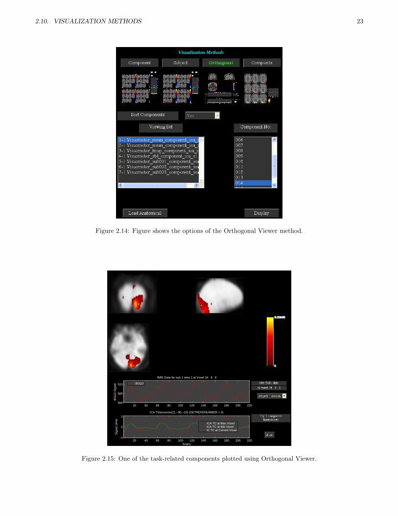
Figure 2.14: Figure shows the options of the Orthogonal Viewer method.
0
9.09649
0
9.09649
0
9.09649
0
9.09649
0
9.09649
0
9.09649
0
9.09649
0
9.09649
0
9.09649
20 40 60 80 100 120 140 160 180 200 220500
505
510
BO
LD S
igna
l
fMRI Data for sub 1 sess 1 at Voxel 34 8 8
20 40 60 80 100 120 140 160 180 200 220−2
0
2
Scans
Sig
nal U
nits
ICA Timecourse(21,−90,−24) (DETRENDNUMBER = 3)
ICA TC at Max VoxelICA TC at Min VoxelIC TC at Current Voxel
BOLD
Figure 2.15: One of the task-related components plotted using Orthogonal Viewer.

24 CHAPTER 2. GETTING STARTED WITH GIFT
Visualization Methods
Figure 2.16: Selected options of the Composite Viewer method.
2.10.3 Orthogonal Explorer
• Orthogonal viewer is used to look at a component and compare it to the functional data.
• Figure 2.14 shows the selected parameters. Click on Display button. Figure 2.15 shows one of the task relatedcomponents.
• Upper plot is the BOLD time course for the selected data-set in the popup window at the current voxel. Youcan interactively select voxel by clicking on any of the slices. Lower plot shows the ICA time course for themaximum voxel (red), minimum voxel (dotted red) and the selected voxel (green).
• When you click on Plot button top five components (of the selected viewing set in Display GUI ) for the selectedvoxel will be displayed. The maximum voxel and the location will be printed to the command prompt. Option(Click on ”Options” menu) is provided in the figure 2.15 to enter the voxel (real world coordinates) instead ofnavigating around the brain.
2.10.4 Composite Viewer
Composite viewer is used to look at multiple components of interest. Use the component explorer to find thetask related components. In the ’Component Number’ user interface control, select the two components that aretask related. At most five different components can be overlaid on one another. Figure 2.16 shows the selectedparameters. We used anatomical image nsingle_subj_T1_2_2_5.nii from folder icatb/icatb_templates. Whenyou click Display button, figure 2.17 will open in a new window.
2.11 Sorting Components
Sorting is a way to classify the components. The components can be sorted either spatially or temporally. For everyindependent component spatial maps and time courses are generated. Temporal sorting is a way to compare themodel’s time course with the ICA time course whereas spatial sorting classifies the components by comparing thecomponent’s image with the template. When you click Component button, ’Sort Components’ popup box will beenabled. Select ’Yes’ for ’Sort Components’. Click Display button then a figure (Figure 2.18) will open in a newwindow. We have implemented three different types of sorting criteria like Correlation, Kurtosis and Multiple Linear

2.11. SORTING COMPONENTS 25
85 80 75 70 65 60
55 50 45 40 35 30
25 20 15 10 5 0
−5 −10 −15 −20 −25 −30
−35 −40 −45 −50
LR
10.7
0
9.5
0
20 40 60 80 100 120 140 160 180 200 220
−1
0
1
Scans
Sig
nal U
nits
−2
0
2IC 14
IC 2
Figure 2.17: Task-related components overlaid on one another. At most five different components with different colorbars can be overlaid.
Regression (MLR). MLR can be a very useful method in separating the two task related components. First, temporalsorting is explained followed by spatial sorting. The following are the steps involved in sorting components:
2.11.1 Temporal Sorting
Multiple regression sorting criteria is used to explain the temporal sorting. We select all data-sets (concatenatedICA time courses) and correlate with model time course. The regressors selected are ”right*bf(1)” and ”left*bf(1)”time courses. After the calculation is done, components are sorted based on the R-square statistic. The R-squarestatistic values and the slopes of the regressors are printed to a text file with the suffix regression.txt. Partialcorrelations and the slopes of the regressors are printed to a text file with the suffix partial_corr.txt. Figure 2.19shows the components sorted based on the MLR sorting criteria in groupings of four. Here you can see that the firsttwo components are task related. For a larger view of the time course plot (Figure 2.20) click on the time courseplot in the main window. A list of menus is plotted on the time course plot. The explanation of each menu will beexplained below:
• Utilities: Utilities contain sub menus like ”Power Spectrum”, ”Split-time courses” and ”Event Average”. Whenyou click ”Split-time courses” sub menu, split of the time courses (Figure 2.21) will be shown. Click on submenu ”Event Average” and select ”right*bf(1)” reference function to plot the event averages (Figure 2.22) ofthe ICA time courses. Explanation of the event average is given in Section 2.12.6.
• Options: ”Options” menu has sub menus like ”Timecourse Options”, and ”Adjust ICA”.
– Timecourse Options: When you click on sub menu ”Timecourse Options”, a new figure window will openthat has options for detrending the ICA time course, model time course and options for event average.Explanation of this figure window is given in the Appendix 4.3. Leave the defaults as shown in the figure.
– Adjust ICA: Option is provided in this sub-menu to remove the variance of other than selected regressor.When you click on sub menu ”Adjust ICA”, a list dialog box will open to select the reference function.For now select the ”right*bf(1)” time course. The ICA time course is adjusted by removing the line fit

26 CHAPTER 2. GETTING STARTED WITH GIFT
Figure 2.18: Selected parameters for sorting the components temporally.
85 80 75 70 65 60
55 50 45 40 35 30
25 20 15 10 5 0
−5 −10 −15 −20 −25 −30
−35 −40 −45 −50
LR
0
9.5
−202
Scans
Component 14 temporal multiple regression = 0.74874
85 80 75 70 65 60
55 50 45 40 35 30
25 20 15 10 5 0
−5 −10 −15 −20 −25 −30
−35 −40 −45 −50
LR
0
10.7
−1012
Scans
Component 2 temporal multiple regression = 0.67748
85 80 75 70 65 60
55 50 45 40 35 30
25 20 15 10 5 0
−5 −10 −15 −20 −25 −30
−35 −40 −45 −50
LR
0
11
−101
Scans
Component 11 temporal multiple regression = 0.43585
85 80 75 70 65 60
55 50 45 40 35 30
25 20 15 10 5 0
−5 −10 −15 −20 −25 −30
−35 −40 −45 −50
LR
0
6.3
−1012
Scans
Component 4 temporal multiple regression = 0.32679
Figure 2.19: Components are sorted based on Multiple Regression criteria in groupings of four.

2.11. SORTING COMPONENTS 27
Figure 2.20: Expanded view of the ”right*bf(1)” time course.
50 100 150 200
−2
−1.5
−1
−0.5
0
0.5
1
1.5
2
2.5
Subject 1
50 100 150 200
−1.5
−1
−0.5
0
0.5
1
1.5
2
2.5
Subject 2
50 100 150 200
−1
−0.5
0
0.5
1
1.5
Subject 3
50 100 150 200
−1.5
−1
−0.5
0
0.5
1
1.5
2
2.5
Mean over subjects + SEM
Figure 2.21: Figure shows the split of the concatenated time courses of all the data-sets. Mean is calculated oversessions and subjects as well as over all data-sets.

28 CHAPTER 2. GETTING STARTED WITH GIFT
5 10 15 20 25 30
−0.5
0
0.5
1
1.5
2
Subject 1
5 10 15 20 25 30
−1
−0.5
0
0.5
1
1.5
2
Subject 2
5 10 15 20 25 30
−0.5
0
0.5
1
1.5
Subject 3
5 10 15 20 25 30−1
−0.5
0
0.5
1
1.5
2
Mean over subjects + SEM
Figure 2.22: Figure shows the event related averages of the selected component for different subjects.
Figure 2.23: Expanded view of ICA time course after removing the variance of other than selected regressor(”left*bf(1)”).

2.11. SORTING COMPONENTS 29
50 100 150 200
−2
−1
0
1
2
3Subject 1
50 100 150 200
−2
−1.5
−1
−0.5
0
0.5
1
1.5
2
2.5
Subject 2
50 100 150 200
−1
−0.5
0
0.5
1
1.5
2Subject 3
50 100 150 200
−2
−1.5
−1
−0.5
0
0.5
1
1.5
2
2.5
Mean over subjects + SEM
Figure 2.24: Figure shows the split of the concatenated time courses of all the data-sets after adjusting.
5 10 15 20 25 30
−0.5
0
0.5
1
1.5
2
Subject 1
5 10 15 20 25 30
−0.5
0
0.5
1
1.5
2
Subject 2
5 10 15 20 25 30
−0.5
0
0.5
1
1.5
Subject 3
5 10 15 20 25 30
−0.5
0
0.5
1
1.5
2
Mean over subjects + SEM
Figure 2.25: Figure shows the event averages of the adjusted ICA time courses.

30 CHAPTER 2. GETTING STARTED WITH GIFT
Table 2.2: Table shows two sorted components parameters. Regression values for each component are shown followedby the beta weight of each condition with the ICA time course.
Component Numbers 7 3Regression Values 0.74876543 0.67747138
Subject 1 Sn(1) right*bf(1) 2.3585817 0.55115175Subject 1 Sn(1) left*bf(1) 0.097659759 2.158409Subject 2 Sn(1) right*bf(1) 2.2468961 0.69208646Subject 2 Sn(1) left*bf(1) 0.40444896 1.3045916Subject 3 Sn(1) right*bf(1) 1.4413982 0.46694756Subject 3 Sn(1) left*bf(1) -0.045741345 1.6667349
of the model with the ICA time course where model contains nuisance parameters and other than theselected reference function. After the ICA time course is adjusted the plot is shown in the expanded viewtime course plot (Figure 2.23). When you click on the sub menu ”Split-time courses” in ”Utilities” menu,a new figure window (Figure 2.24) showing the split of the adjusted ICA time courses will be shown.Similarly click on sub menu ”Event-Average” in ”Utilities” menu and select the ”right*bf(1)” referencefunction to view the event averages (Figure 2.25) of the new ICA time courses.
Note: Event average can also be done without sorting components (Section 2.12.6). Please see Appendix 4.2 forentering regressors through a text file for large data-sets.
Statistical Testing Of Images and Time Courses
Two Sample t-test: Two sample t-test can be used to compare a component between subjects or sessions. Forexample for a particular component session 1 images can be treated as group 1 and session 2 images as group 2. Youcan use these images in SPM to do two sample t-test ([11], pp 12-14).
Regression Parameters: After performing temporal sorting, the fit regression parameters are saved in a file withsuffix regression.txt. This file can be quite useful in performing statistical tests to evaluate the task-relatednessof the components or to perform tests between components or groups. The text file contains a number for eachcomponent, regressor, subject and session (Table 2.2). The numbers represent the ’fit parameter’ from the regression.In order to use these numbers it is important to scale the ICA data. For example, if 10 subjects were analyzed withICA and two regressors were used to sort, then one can test the degree to which the average amplitude of group 1was greater than the average amplitude of group 2 by computing a two-sample t-test between the 10 parameters forgroup 1 and the 10 parameters for group 2. A separate test can be done for each component, and the componentwhich show a significant difference can be determined.Note:
• We provide an option in GIFT to do one sample t-test and two sample t-test on individual subject componentmaps using SPM5 (Section 2.13.1).
• We provide utility to do statistics on the regression parameters. Please see section 2.12.9 for more information.
2.11.2 Spatial Sorting
Components can be spatially sorted by defining the regions of interest or a spatial template. Presently, there arefour ways of sorting the components spatially like Multiple Regression, Correlation, Kurtosis and Maximum Voxel.
• ’Select Sorting Criteria’
– The options available are ’Multiple Regression’, ’Correlation’, ’Kurtosis’ and ’Maximum Voxel’. Kurtosiscriteria does not need a template for sorting the components. Multiple Regression criteria can be used toselect one or more templates.
• ’Select Sorting Type’
2.12. UTILITIES 31
85 80 75 70 65 60
55 50 45 40 35 30
25 20 15 10 5 0
−5 −10 −15 −20 −25 −30
−35 −40 −45 −50
LR
0
12
−1012
Scans
Component 2 spatial multiple regression = 0.59971
85 80 75 70 65 60
55 50 45 40 35 30
25 20 15 10 5 0
−5 −10 −15 −20 −25 −30
−35 −40 −45 −50
LR
0
13.2
−202
Scans
Component 14 spatial multiple regression = 0.57538
85 80 75 70 65 60
55 50 45 40 35 30
25 20 15 10 5 0
−5 −10 −15 −20 −25 −30
−35 −40 −45 −50
LR
0
7
−0.500.5
Scans
Component 7 spatial multiple regression = 0.039339
85 80 75 70 65 60
55 50 45 40 35 30
25 20 15 10 5 0
−5 −10 −15 −20 −25 −30
−35 −40 −45 −50
LR
0
12.8
−101
Scans
Component 12 spatial multiple regression = 0.026323
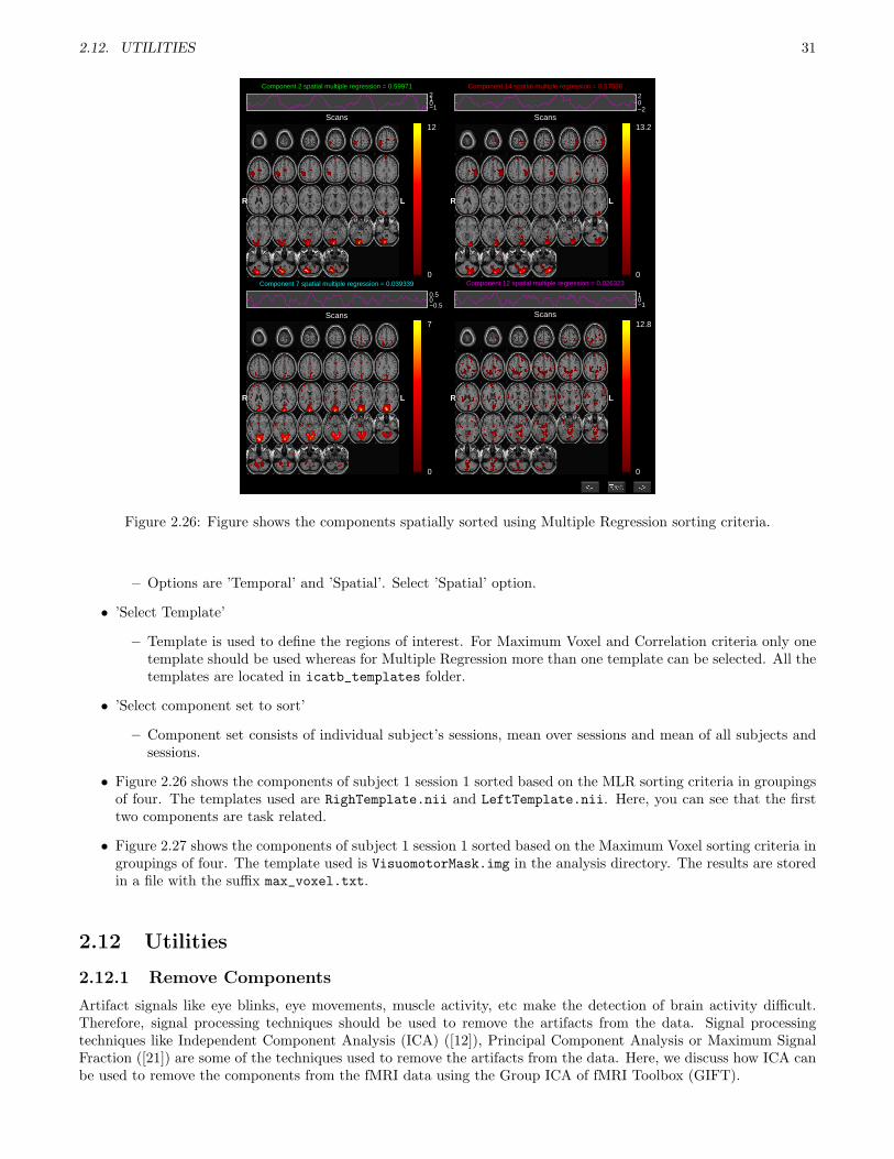
Figure 2.26: Figure shows the components spatially sorted using Multiple Regression sorting criteria.
– Options are ’Temporal’ and ’Spatial’. Select ’Spatial’ option.
• ’Select Template’
– Template is used to define the regions of interest. For Maximum Voxel and Correlation criteria only onetemplate should be used whereas for Multiple Regression more than one template can be selected. All thetemplates are located in icatb_templates folder.
• ’Select component set to sort’
– Component set consists of individual subject’s sessions, mean over sessions and mean of all subjects andsessions.
• Figure 2.26 shows the components of subject 1 session 1 sorted based on the MLR sorting criteria in groupingsof four. The templates used are RighTemplate.nii and LeftTemplate.nii. Here, you can see that the firsttwo components are task related.
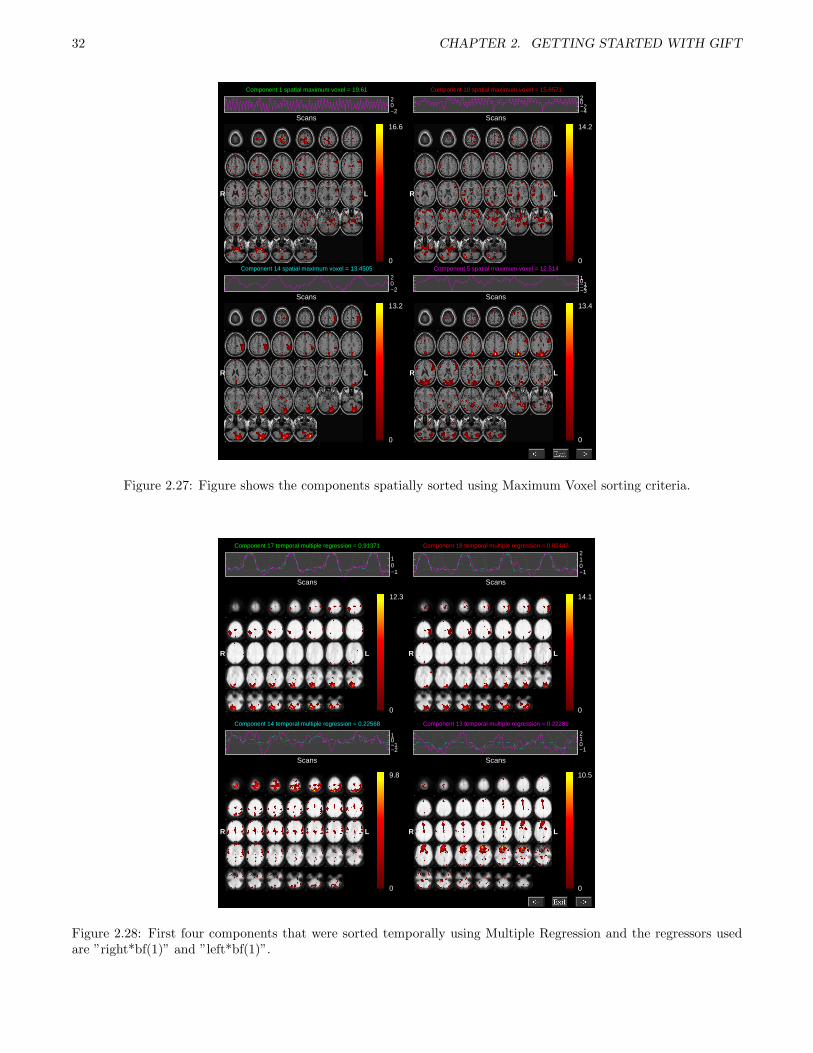
• Figure 2.27 shows the components of subject 1 session 1 sorted based on the Maximum Voxel sorting criteria ingroupings of four. The template used is VisuomotorMask.img in the analysis directory. The results are storedin a file with the suffix max_voxel.txt.
2.12 Utilities
2.12.1 Remove Components
Artifact signals like eye blinks, eye movements, muscle activity, etc make the detection of brain activity difficult.Therefore, signal processing techniques should be used to remove the artifacts from the data. Signal processingtechniques like Independent Component Analysis (ICA) ([12]), Principal Component Analysis or Maximum SignalFraction ([21]) are some of the techniques used to remove the artifacts from the data. Here, we discuss how ICA canbe used to remove the components from the fMRI data using the Group ICA of fMRI Toolbox (GIFT).
32 CHAPTER 2. GETTING STARTED WITH GIFT
85 80 75 70 65 60
55 50 45 40 35 30
25 20 15 10 5 0
−5 −10 −15 −20 −25 −30
−35 −40 −45 −50
LR
0
16.6
−202
Scans
Component 1 spatial maximum voxel = 19.61
85 80 75 70 65 60
55 50 45 40 35 30
25 20 15 10 5 0
−5 −10 −15 −20 −25 −30
−35 −40 −45 −50
LR
0
14.2
−4−202
Scans
Component 10 spatial maximum voxel = 15.6571
85 80 75 70 65 60
55 50 45 40 35 30
25 20 15 10 5 0
−5 −10 −15 −20 −25 −30
−35 −40 −45 −50
LR
0
13.2
−202
Scans
Component 14 spatial maximum voxel = 13.4505
85 80 75 70 65 60
55 50 45 40 35 30
25 20 15 10 5 0
−5 −10 −15 −20 −25 −30
−35 −40 −45 −50
LR
0
13.4
−3−2−101
Scans
Component 5 spatial maximum voxel = 12.514
Figure 2.27: Figure shows the components spatially sorted using Maximum Voxel sorting criteria.
80 76 72 68 64 60 56
52 48 44 40 36 32 28
24 20 16 12 8 4 0
−4 −8 −12 −16 −20 −24 −28
−32 −36 −40 −44 −48 −52
LR
0
12.3
−101
Scans
Component 17 temporal multiple regression = 0.91371
80 76 72 68 64 60 56
52 48 44 40 36 32 28
24 20 16 12 8 4 0
−4 −8 −12 −16 −20 −24 −28
−32 −36 −40 −44 −48 −52
LR
0
14.1
−1012
Scans
Component 18 temporal multiple regression = 0.82442
80 76 72 68 64 60 56
52 48 44 40 36 32 28
24 20 16 12 8 4 0
−4 −8 −12 −16 −20 −24 −28
−32 −36 −40 −44 −48 −52
LR
0
9.8
−2−101
Scans
Component 14 temporal multiple regression = 0.22568
80 76 72 68 64 60 56
52 48 44 40 36 32 28
24 20 16 12 8 4 0
−4 −8 −12 −16 −20 −24 −28
−32 −36 −40 −44 −48 −52
LR
0
10.5
−1012
Scans
Component 13 temporal multiple regression = 0.22281
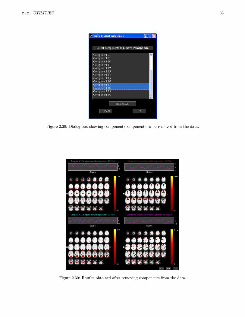
Figure 2.28: First four components that were sorted temporally using Multiple Regression and the regressors usedare ”right*bf(1)” and ”left*bf(1)”.
2.12. UTILITIES 33
Figure 2.29: Dialog box showing component/components to be removed from the data.
80 76 72 68 64 60 56
52 48 44 40 36 32 28
24 20 16 12 8 4 0
−4 −8 −12 −16 −20 −24 −28
−32 −36 −40 −44 −48 −52
LR
0
10.1
−2
0
2
Scans
Component 17 temporal multiple regression = 0.22706
80 76 72 68 64 60 56
52 48 44 40 36 32 28
24 20 16 12 8 4 0
−4 −8 −12 −16 −20 −24 −28
−32 −36 −40 −44 −48 −52
LR
0
10.5
−2
0
2
Scans
Component 13 temporal multiple regression = 0.21988
80 76 72 68 64 60 56
52 48 44 40 36 32 28
24 20 16 12 8 4 0
−4 −8 −12 −16 −20 −24 −28
−32 −36 −40 −44 −48 −52
LR
0
7.1
−2
0
2
Scans
Component 11 temporal multiple regression = 0.15694
80 76 72 68 64 60 56
52 48 44 40 36 32 28
24 20 16 12 8 4 0
−4 −8 −12 −16 −20 −24 −28
−32 −36 −40 −44 −48 −52
LR
0
11.4
−2
0
2
Scans
Component 12 temporal multiple regression = 0.094639
Figure 2.30: Results obtained after removing components from the data.

34 CHAPTER 2. GETTING STARTED WITH GIFT
−40 −36 −32 −28 −24
−20 −16 −12 −8 −4
+0 +4 +8 +12 +16
+20 +24 +28 +32 +36
+40 +44 +48 +52 +56
+60 +64 +68 +72
5
10
15
20
Figure 2.31: Left-right visual before removing the IC from the data.
• ICA was run on single subject single session and 20 components are extracted from the data. After the ICAanalysis, the components extracted form a derived measure of the data. In order to remove artifacts, identifythe components using any of the visualization methods used in the toolbox (Figure 2.1). Here, we remove thetask-related components and these are identified by sorting components temporally.
• After identifying the components, use the ”Utilities” drop down box and select ”Remove Component(s)” entry.A figure window will open to select the parameter file used for the analysis. This is the same parameter filethat you have used for running ICA on the fMRI data.
• After the parameter file is selected, a list dialog box (Figure 2.29) will open to select the components to beremoved from the fMRI Data. We selected the first two components in the figure 2.28 to be removed from thedata. The components will be removed from the data by zeroing out the corresponding columns of the mixingmatrix and the rows of the spatial maps. The modified data is written to the selected output directory. Thenew set of images will have prefix R_.
• The modified data can now be analyzed using any toolbox that analyzes fMRI data. ICA is used to analyzethe modified data and the components are sorted temporally using Multiple Regression and the regressorsselected are ”right*bf(1)” and the ”left*bf(1)”. Figure 2.30 shows that both left and right visual componentsare removed from the data.
2.12. UTILITIES 35
−40 −36 −32 −28 −24
−20 −16 −12 −8 −4
+0 +4 +8 +12 +16
+20 +24 +28 +32 +36
+40 +44 +48 +52 +56
+60 +64 +68 +72
4
5
6
7
8
9
Figure 2.32: Left-right visual after removing the IC from the data.
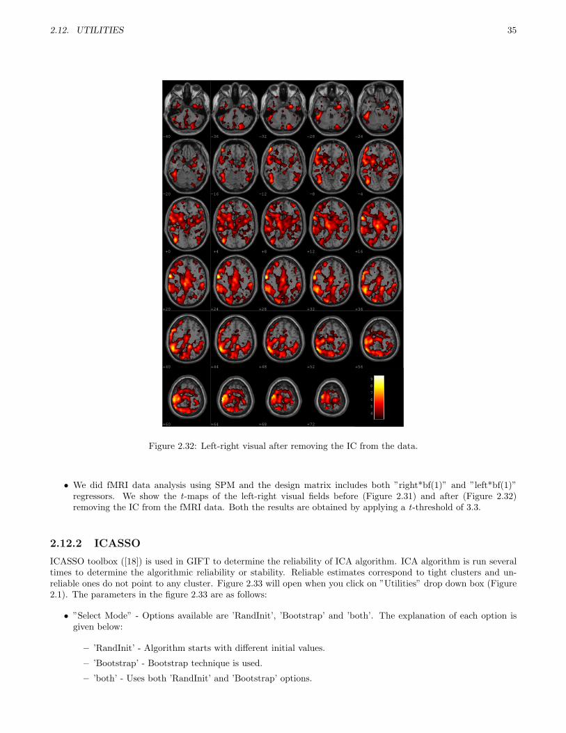
• We did fMRI data analysis using SPM and the design matrix includes both ”right*bf(1)” and ”left*bf(1)”regressors. We show the t-maps of the left-right visual fields before (Figure 2.31) and after (Figure 2.32)removing the IC from the fMRI data. Both the results are obtained by applying a t-threshold of 3.3.
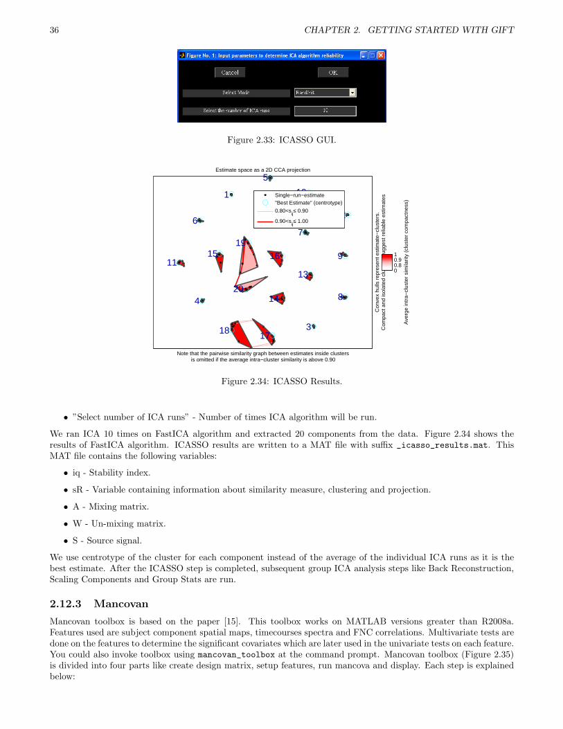
2.12.2 ICASSO
ICASSO toolbox ([18]) is used in GIFT to determine the reliability of ICA algorithm. ICA algorithm is run severaltimes to determine the algorithmic reliability or stability. Reliable estimates correspond to tight clusters and un-reliable ones do not point to any cluster. Figure 2.33 will open when you click on ”Utilities” drop down box (Figure2.1). The parameters in the figure 2.33 are as follows:
• ”Select Mode” - Options available are ’RandInit’, ’Bootstrap’ and ’both’. The explanation of each option isgiven below:
– ’RandInit’ - Algorithm starts with different initial values.
– ’Bootstrap’ - Bootstrap technique is used.
– ’both’ - Uses both ’RandInit’ and ’Bootstrap’ options.
36 CHAPTER 2. GETTING STARTED WITH GIFT
Figure 2.33: ICASSO GUI.
Estimate space as a 2D CCA projection
1
2
3
4
5
6 7
8
9
10
11
12
13
14
15 16
1718
19
20
Note that the pairwise similarity graph between estimates inside clustersis omitted if the average intra−cluster similarity is above 0.90
Con
vex
hulls
rep
rese
nt e
stim
ate−
clus
ters
.C
ompa
ct a
nd is
olat
ed c
lust
ers
sugg
est r
elia
ble
estim
ates
Ave
rge
intr
a−cl
uste
r si
mila
rity
(clu
ster
com
pact
ness
)
00.80.91
Single−run−estimate"Best Estimate" (centrotype)
0.80<sij≤ 0.90
0.90<sij≤ 1.00
Figure 2.34: ICASSO Results.
• ”Select number of ICA runs” - Number of times ICA algorithm will be run.
We ran ICA 10 times on FastICA algorithm and extracted 20 components from the data. Figure 2.34 shows theresults of FastICA algorithm. ICASSO results are written to a MAT file with suffix _icasso_results.mat. ThisMAT file contains the following variables:
• iq - Stability index.
• sR - Variable containing information about similarity measure, clustering and projection.
• A - Mixing matrix.
• W - Un-mixing matrix.
• S - Source signal.
We use centrotype of the cluster for each component instead of the average of the individual ICA runs as it is thebest estimate. After the ICASSO step is completed, subsequent group ICA analysis steps like Back Reconstruction,Scaling Components and Group Stats are run.
2.12.3 Mancovan
Mancovan toolbox is based on the paper [15]. This toolbox works on MATLAB versions greater than R2008a.Features used are subject component spatial maps, timecourses spectra and FNC correlations. Multivariate tests aredone on the features to determine the significant covariates which are later used in the univariate tests on each feature.You could also invoke toolbox using mancovan_toolbox at the command prompt. Mancovan toolbox (Figure 2.35)is divided into four parts like create design matrix, setup features, run mancova and display. Each step is explainedbelow:
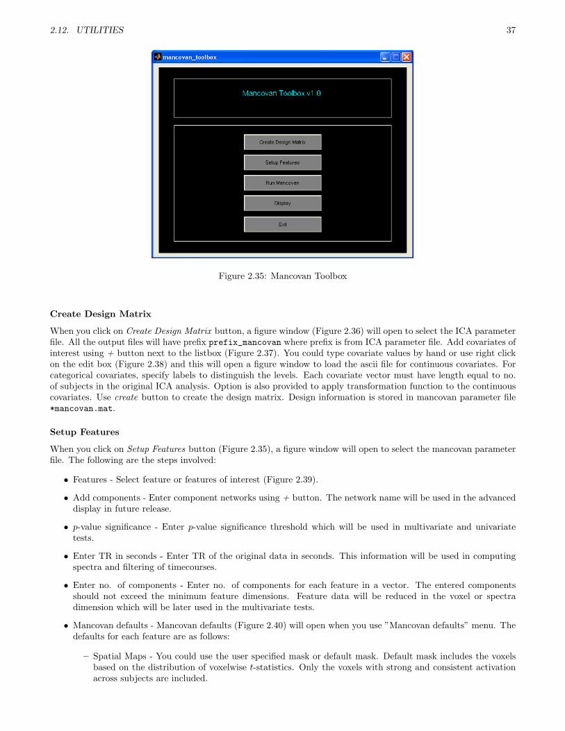
2.12. UTILITIES 37
Figure 2.35: Mancovan Toolbox
Create Design Matrix
When you click on Create Design Matrix button, a figure window (Figure 2.36) will open to select the ICA parameterfile. All the output files will have prefix prefix_mancovan where prefix is from ICA parameter file. Add covariates ofinterest using + button next to the listbox (Figure 2.37). You could type covariate values by hand or use right clickon the edit box (Figure 2.38) and this will open a figure window to load the ascii file for continuous covariates. Forcategorical covariates, specify labels to distinguish the levels. Each covariate vector must have length equal to no.of subjects in the original ICA analysis. Option is also provided to apply transformation function to the continuouscovariates. Use create button to create the design matrix. Design information is stored in mancovan parameter file*mancovan.mat.
Setup Features
When you click on Setup Features button (Figure 2.35), a figure window will open to select the mancovan parameterfile. The following are the steps involved:
• Features - Select feature or features of interest (Figure 2.39).
• Add components - Enter component networks using + button. The network name will be used in the advanceddisplay in future release.
• p-value significance - Enter p-value significance threshold which will be used in multivariate and univariatetests.
• Enter TR in seconds - Enter TR of the original data in seconds. This information will be used in computingspectra and filtering of timecourses.
• Enter no. of components - Enter no. of components for each feature in a vector. The entered componentsshould not exceed the minimum feature dimensions. Feature data will be reduced in the voxel or spectradimension which will be later used in the multivariate tests.
• Mancovan defaults - Mancovan defaults (Figure 2.40) will open when you use ”Mancovan defaults” menu. Thedefaults for each feature are as follows:
– Spatial Maps - You could use the user specified mask or default mask. Default mask includes the voxelsbased on the distribution of voxelwise t-statistics. Only the voxels with strong and consistent activationacross subjects are included.

38 CHAPTER 2. GETTING STARTED WITH GIFT
Figure 2.36: Figure window to select the ICA parameter file
Figure 2.37: Setup Mancovan Design

2.12. UTILITIES 39
Figure 2.38: Add covariates
Figure 2.39: Setup features for mancovan analysis
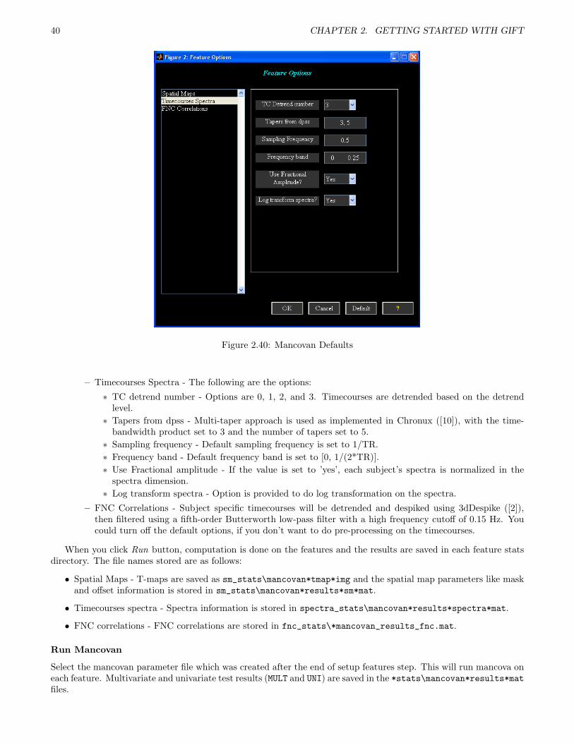
40 CHAPTER 2. GETTING STARTED WITH GIFT
Figure 2.40: Mancovan Defaults
– Timecourses Spectra - The following are the options:
∗ TC detrend number - Options are 0, 1, 2, and 3. Timecourses are detrended based on the detrendlevel.
∗ Tapers from dpss - Multi-taper approach is used as implemented in Chronux ([10]), with the time-bandwidth product set to 3 and the number of tapers set to 5.
∗ Sampling frequency - Default sampling frequency is set to 1/TR.
∗ Frequency band - Default frequency band is set to [0, 1/(2*TR)].
∗ Use Fractional amplitude - If the value is set to ’yes’, each subject’s spectra is normalized in thespectra dimension.
∗ Log transform spectra - Option is provided to do log transformation on the spectra.
– FNC Correlations - Subject specific timecourses will be detrended and despiked using 3dDespike ([2]),then filtered using a fifth-order Butterworth low-pass filter with a high frequency cutoff of 0.15 Hz. Youcould turn off the default options, if you don’t want to do pre-processing on the timecourses.
When you click Run button, computation is done on the features and the results are saved in each feature statsdirectory. The file names stored are as follows:
• Spatial Maps - T-maps are saved as sm_stats\mancovan*tmap*img and the spatial map parameters like maskand offset information is stored in sm_stats\mancovan*results*sm*mat.
• Timecourses spectra - Spectra information is stored in spectra_stats\mancovan*results*spectra*mat.
• FNC correlations - FNC correlations are stored in fnc_stats\*mancovan_results_fnc.mat.
Run Mancovan
Select the mancovan parameter file which was created after the end of setup features step. This will run mancova oneach feature. Multivariate and univariate test results (MULT and UNI) are saved in the *stats\mancovan*results*matfiles.

2.12. UTILITIES 41
Figure 2.41: Display Mancovan Results
Figure 2.42: T-map and Spectra

42 CHAPTER 2. GETTING STARTED WITH GIFT
Figure 2.43: FNC Correlations
Figure 2.44: Multivariate results
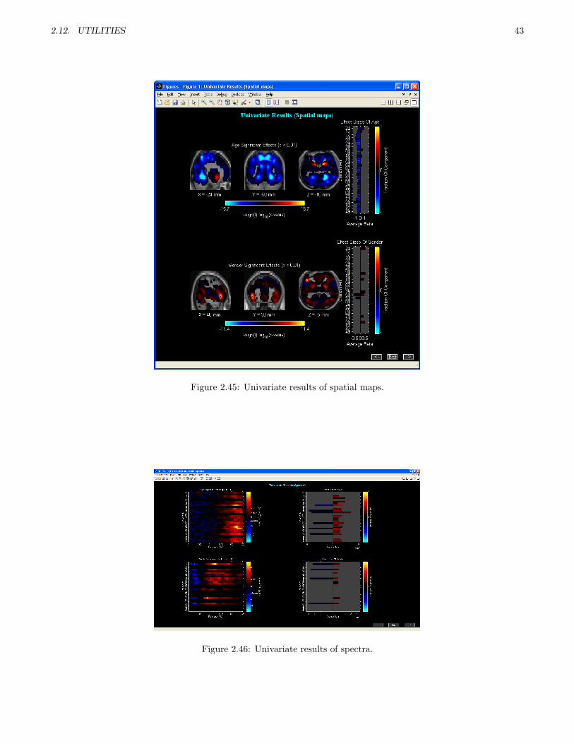
2.12. UTILITIES 43
Figure 2.45: Univariate results of spatial maps.
Figure 2.46: Univariate results of spectra.

44 CHAPTER 2. GETTING STARTED WITH GIFT
Figure 2.47: Univariate results of FNC.
Display
When you click Display button (Figure 2.35), Figure 2.41 will open.
• Features - Features will be displayed when you select features and click on display button. Figures 2.42 and2.43 show ortho views of T-maps, power spectra, and FNC correlations. T-maps are thresholded using thesame threshold as selected in the Setup Features option and you can interactively browse using mouse withineach slice.
• Multivariate results - Significant results of covariates will be plotted in a matrix of dimensions covariates bycomponents (Figure 2.44). The darker the color the more significant is the covariate in that component.
• Univariate results - Univariate results of age and gender covariates are shown for each feature in figures 2.45,2.46 and 2.47.
– Spatial maps - On the left side of the plot (Figure 2.45), composite maps of significant effects over allcomponents are displayed as −sign(t)log10(p). Effects are considered significant if test statistics exceededthe FDR threshold (α = 0.01) with a cluster extent of at least 27 contiguous voxels. Plots on the right sideshow average β values. β-values are averaged over significant clusters with effects of the same directionalityand the color of the bar is proportional to the fraction of component voxels contributing to each effect.
– Timecourses spectra - On the left side of the plot (Figure 2.46), covariates significance is shown as afunction of frequency for each component displayed as −sign(t)log10(p). Dashed horizontal lines on thecolorbar designate the FDR corrected threshold (α = 0.01). On the right side of the plot, β-values areaveraged over frequency bands with effects of the same directionality where test statistics exceeded theFDR threshold. The color of the bar is proportional to the fraction of contributing frequency bins. Theabsence of a bar indicates that univariate tests were not performed or test statistics were not significant.
– FNC Correlations - Significance and direction of age and gender terms for each pairwise correlation,displayed as the −sign(t)log10(p). Dashed horizontal lines on the colorbar designate the FDR correctedthreshold (α = 0.01).
2.12.4 dFNC
Dynamic FNC toolbox (dFNC) is used to study function network connectivity dynamics. dFNC toolbox computeswindowed correlation matrices from component time courses and offers approaches to estimate stable connectivitystates ([13]). This toolbox works on MATLAB versions greater than R2008a. dFNC toolbox could be invoked byusing ”Utilities” drop down box under GIFT main figure window (Figure 2.1) or by using command dfnc_toolbox atthe command prompt. dFNC toolbox (Figure 2.48) is divided into three parts like Setup/Run dFNC, Post-proecssingand Display. Each step is explained below:

2.12. UTILITIES 45
Figure 2.48: dFNC Toolbox
Figure 2.49: Setup/Run dFNC
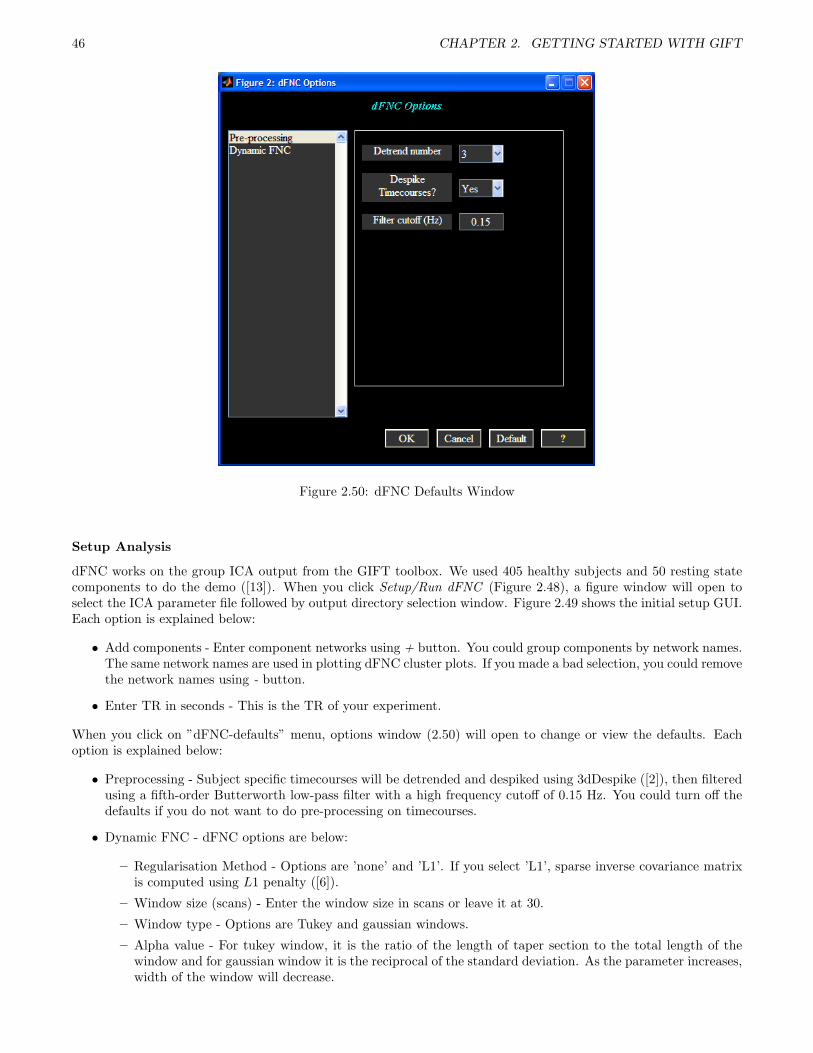
46 CHAPTER 2. GETTING STARTED WITH GIFT
Figure 2.50: dFNC Defaults Window
Setup Analysis
dFNC works on the group ICA output from the GIFT toolbox. We used 405 healthy subjects and 50 resting statecomponents to do the demo ([13]). When you click Setup/Run dFNC (Figure 2.48), a figure window will open toselect the ICA parameter file followed by output directory selection window. Figure 2.49 shows the initial setup GUI.Each option is explained below:
• Add components - Enter component networks using + button. You could group components by network names.The same network names are used in plotting dFNC cluster plots. If you made a bad selection, you could removethe network names using - button.
• Enter TR in seconds - This is the TR of your experiment.
When you click on ”dFNC-defaults” menu, options window (2.50) will open to change or view the defaults. Eachoption is explained below:
• Preprocessing - Subject specific timecourses will be detrended and despiked using 3dDespike ([2]), then filteredusing a fifth-order Butterworth low-pass filter with a high frequency cutoff of 0.15 Hz. You could turn off thedefaults if you do not want to do pre-processing on timecourses.
• Dynamic FNC - dFNC options are below:
– Regularisation Method - Options are ’none’ and ’L1’. If you select ’L1’, sparse inverse covariance matrixis computed using L1 penalty ([6]).
– Window size (scans) - Enter the window size in scans or leave it at 30.
– Window type - Options are Tukey and gaussian windows.
– Alpha value - For tukey window, it is the ratio of the length of taper section to the total length of thewindow and for gaussian window it is the reciprocal of the standard deviation. As the parameter increases,width of the window will decrease.

2.12. UTILITIES 47
Figure 2.51: Post-processing Window
– No. of repetitions (L1 regularisation) - No. of times the timecourses are trained to get a better estimatesof Lambda which will be used in L1 regularisation.
After completing the parameters selection, use Run (Figure 2.48) to run the dynamic FNC. Windowed correlationmatrices are saved for each subject in variable FNCdyn in file prefix_sub_*_results.mat. dFNC parameters aresaved in variable dfncInfo in file prefix_dfnc.mat where prefix is the same prefix you gave during the ICAanalysis.
Post-processing
Figure 2.51 will open when you click on Post-processing button (Figure 2.48). K-means is computed on the windowedFNC correlations. Percentage of number of occurrences of the cluster over the total number of occurrences is reportedfor each cluster state. At the end of the post-processing step, results are saved in file _post_process.mat.
Display
Display GUI includes options to display FNC spectra and cluster centroids. When you click on Display button(Figure 2.48), display window (Figure 2.52) will open. There are two options like ”FNC Oscillations and ”Clusterstats” (Figure 2.52).
• FNC Oscillations - Average standard deviation of spectra and average spectral central of mass are computed.Figure 2.53 shows the average standard deviation of FNC spectra across subjects.
• Cluster stats - K-means is computed on the windowed correlations and 6 clusters are selected. Figure 2.54shows one of the cluster centroids. Title shows percentage of number of occurrences of the cluster over thetotal number of occurrences. Figure 2.55 shows the frequency of each cluster, mean dwell time in windows foreach cluster and state transition matrix.
Note: HTML report is created in html directory when you click on ”HTML” menu in display GUI (Figure 2.52.
2.12.5 Ascii to SPM.mat
Temporal sorting is done using a SPM (SPM2 or SPM5) design matrix. You can create SPM design matrix from aascii file containing regressor time courses using ”Utilities” (Figure 2.1) drop down box. Under ”Utilities” drop downbox select Ascii_to_spm.mat. The time course matrix is of dimensions m by n where m is the sum of the numberof scans over sessions and n is the number of total regressors. Type help icatb_formDesignMat at the MATLABcommand prompt for an example. See icatb_templates folder for example regressor data files.
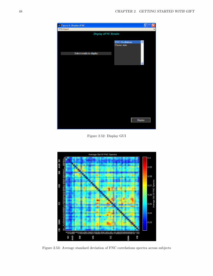
48 CHAPTER 2. GETTING STARTED WITH GIFT
Figure 2.52: Display GUI
Average Std Of FNC Spectra
8 13 15 57 98 99 2 9 10 14 30 37 45 58 27 43 46 60 77 79 80 82 89 21 29 36 47 56 59 61 66 67 71 76 81 88 90 93 20 26 28 39 44 48 64 75 87 7 12 32
SC
AU
DS
MV
ISC
CD
MN
CB
SC
AU
D
SM
VIS CC
DM
N
CB
12
34
56
78
910
1112
1314
1516
1718
1920
2122
2324
2526
2728
2930
3132
3334
3536
3738
3940
4142
4344
4546
4748
4950
81315579899 2 9101430374558274346607779808289212936475659616667717681889093202628394448647587 71232
Ave
rage
Std
Of F
NC
Spe
ctra
0.23
0.24
0.25
0.26
0.27
0.28
0.29
0.3
Figure 2.53: Average standard deviation of FNC correlations spectra across subjects
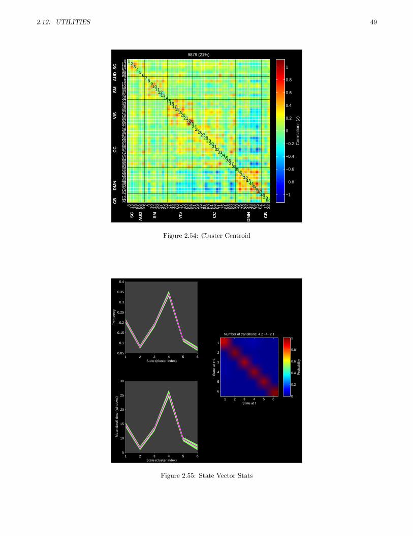
2.12. UTILITIES 49
9879 (21%)
8 13 15 57 98 99 2 9 10 14 30 37 45 58 27 43 46 60 77 79 80 82 89 21 29 36 47 56 59 61 66 67 71 76 81 88 90 93 20 26 28 39 44 48 64 75 87 7 12 32
SC
AU
DS
MV
ISC
CD
MN
CB
SC
AU
D
SM
VIS CC
DM
N
CB
12
34
56
78
910
1112
1314
1516
1718
1920
2122
2324
2526
2728
2930
3132
3334
3536
3738
3940
4142
4344
4546
4748
4950
81315579899 2 9101430374558274346607779808289212936475659616667717681889093202628394448647587 71232
Cor
rela
tions
(z)
−1
−0.8
−0.6
−0.4
−0.2
0
0.2
0.4
0.6
0.8
1
Figure 2.54: Cluster Centroid
1 2 3 4 5 60.05
0.1
0.15
0.2
0.25
0.3
0.35
0.4
State (cluster index)
Fre
quen
cy
1 2 3 4 5 65
10
15
20
25
30
State (cluster index)
Mea
n dw
ell t
ime
(win
dow
s)
State at t
Sta
te a
t t−
1
Number of transitions: 4.2 +/− 2.1
1 2 3 4 5 6
1
2
3
4
5
6
Pro
babi
lity
0
0.2
0.4
0.6
0.8
1
Figure 2.55: State Vector Stats
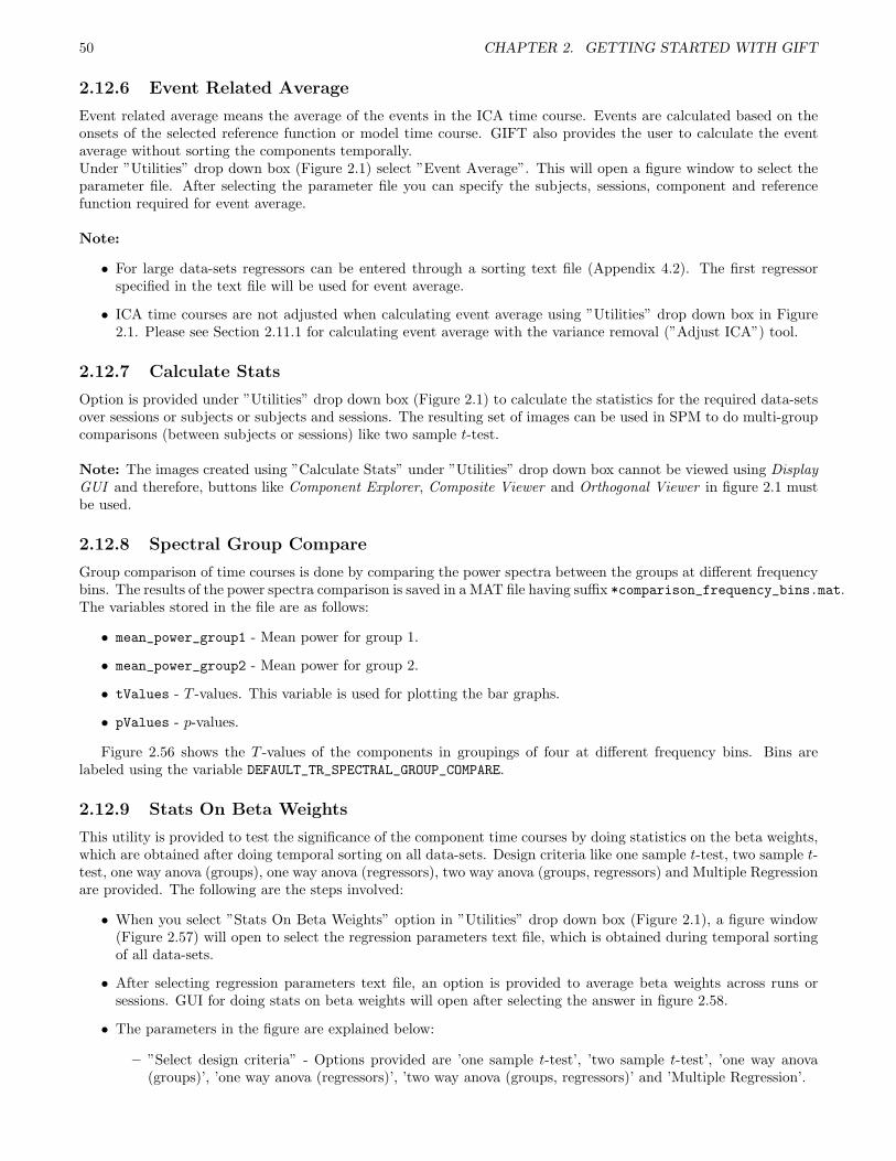
50 CHAPTER 2. GETTING STARTED WITH GIFT
2.12.6 Event Related Average
Event related average means the average of the events in the ICA time course. Events are calculated based on theonsets of the selected reference function or model time course. GIFT also provides the user to calculate the eventaverage without sorting the components temporally.Under ”Utilities” drop down box (Figure 2.1) select ”Event Average”. This will open a figure window to select theparameter file. After selecting the parameter file you can specify the subjects, sessions, component and referencefunction required for event average.
Note:
• For large data-sets regressors can be entered through a sorting text file (Appendix 4.2). The first regressorspecified in the text file will be used for event average.
• ICA time courses are not adjusted when calculating event average using ”Utilities” drop down box in Figure2.1. Please see Section 2.11.1 for calculating event average with the variance removal (”Adjust ICA”) tool.
2.12.7 Calculate Stats
Option is provided under ”Utilities” drop down box (Figure 2.1) to calculate the statistics for the required data-setsover sessions or subjects or subjects and sessions. The resulting set of images can be used in SPM to do multi-groupcomparisons (between subjects or sessions) like two sample t-test.
Note: The images created using ”Calculate Stats” under ”Utilities” drop down box cannot be viewed using DisplayGUI and therefore, buttons like Component Explorer, Composite Viewer and Orthogonal Viewer in figure 2.1 mustbe used.
2.12.8 Spectral Group Compare
Group comparison of time courses is done by comparing the power spectra between the groups at different frequencybins. The results of the power spectra comparison is saved in a MAT file having suffix *comparison_frequency_bins.mat.The variables stored in the file are as follows:
• mean_power_group1 - Mean power for group 1.
• mean_power_group2 - Mean power for group 2.
• tValues - T -values. This variable is used for plotting the bar graphs.
• pValues - p-values.
Figure 2.56 shows the T -values of the components in groupings of four at different frequency bins. Bins arelabeled using the variable DEFAULT_TR_SPECTRAL_GROUP_COMPARE.
2.12.9 Stats On Beta Weights
This utility is provided to test the significance of the component time courses by doing statistics on the beta weights,which are obtained after doing temporal sorting on all data-sets. Design criteria like one sample t-test, two sample t-test, one way anova (groups), one way anova (regressors), two way anova (groups, regressors) and Multiple Regressionare provided. The following are the steps involved:
• When you select ”Stats On Beta Weights” option in ”Utilities” drop down box (Figure 2.1), a figure window(Figure 2.57) will open to select the regression parameters text file, which is obtained during temporal sortingof all data-sets.
• After selecting regression parameters text file, an option is provided to average beta weights across runs orsessions. GUI for doing stats on beta weights will open after selecting the answer in figure 2.58.
• The parameters in the figure are explained below:
– ”Select design criteria” - Options provided are ’one sample t-test’, ’two sample t-test’, ’one way anova(groups)’, ’one way anova (regressors)’, ’two way anova (groups, regressors)’ and ’Multiple Regression’.

2.12. UTILITIES 51
0.04 0.08 0.12 0.16 0.2 0.24−4
−2
0
2
4
6
8
T−
Val
ues
Frequency (Hz)
HE − SZ
Comp 1Comp 2Comp 3Comp 4
0.04 0.08 0.12 0.16 0.2 0.24−10
−5
0
5
T−
Val
ues
Frequency (Hz)
HE − SZ
Comp 5Comp 6Comp 7Comp 8
0.04 0.08 0.12 0.16 0.2 0.24−8
−6
−4
−2
0
2
4
T−
Val
ues
Frequency (Hz)
HE − SZ
Comp 9Comp 10Comp 11Comp 12
0.04 0.08 0.12 0.16 0.2 0.24−7
−6
−5
−4
−3
−2
−1
0
1
2
3
T−
Val
ues
Frequency (Hz)
HE − SZ
Comp 13Comp 14Comp 15Comp 16
Figure 2.56: Power spectra difference between groups.
Figure 2.57: Figure window used to select the regression parameters text file.

52 CHAPTER 2. GETTING STARTED WITH GIFT
Figure 2.58: Option for averaging beta weights across runs or sessions.
Figure 2.59: Figure window used to enter group name, subject and session numbers for a group.

2.12. UTILITIES 53
Figure 2.60: Figure window used to enter contrast name and vector.
Figure 2.61: GUI shows the completed parameters.
Figure 2.62: Option for doing operation on selected regressors.

54 CHAPTER 2. GETTING STARTED WITH GIFT
– Groups Listbox - You can add groups using + button adjacent to groups listbox. Figure 2.59 will opento select subjects and sessions for that group. You can also use edit box below the listbox to select thesubjects, if the subject numbers are stored in ascii file by entering load(’c:\sub1.asc’) or using anyother valid MATLAB expression. Each group added will be an entry in groups listbox. You need todouble click on the entry or press enter key to view or make any changes to the selected group. To removethe selected groups use - button adjacent to groups listbox.
– Regressors Listbox - You can select only one regressor for one sample t-test and two sample t-test whereasfor Anova and Multiple Regression you can select multiple regressors.
– Contrasts Listbox - This option is provided to do Anova contrasts. To add a contrast use + button (Figure2.60) adjacent to contrasts listbox. Sum of contrast vector must equal to zero. The length of contrastvector to enter will change depending on the design criteria. The description is as follows:
∗ One way anova (Groups) - Length of contrast vector is equal to the number of selected groups. Forexample if there are 2 groups contrast vector must be of length 2.
∗ One way anova (Regressors) - Length of contrast vector is equal to the number of selected regressors.For example if there are 4 regressors contrast vector must be of length 4.
∗ Two way anova (Groups, Regressors) - Length of contrast vector is equal to the number of selectedgroups and regressors. For example if there are 2 groups and 4 regressors, contrast vector must be oflength 6. First 2 entries correspond to groups and the next 4 entries correspond to regressors.
Note: You need to use double click or press enter key on the selected contrast, if you decide to changethe name of the contrast or value of the contrast vector.
• Calculate - Statistics are done after selecting the design criteria, groups, regressors and contrasts (Figure 2.61).All the results are printed to a file with suffix summary.txt. This file also contains mean and standard deviationfor each condition of a group. An additional option is provided for one way anova (groups) to do operation onregressors (Figure 2.62) and treat it as a single regressor. For example, if you have selected two regressors liketargets and novels to test the significance of components. You can directly subtract targets and novels and doa one way anova (groups) by specifying [1 -1] for the equation of regressors.
Note:
• When you select Multiple regression tool, a figure window will open to select the regressor file or files like age,test scores, etc. After you selected the regressor files, R-square statistic is calculated for each component. Wealso report the slopes and partial correlations of the regressors.
• Option is provided to do statistics on the beta weights using a batch file. Please see section 2.13.1 for moreinformation.
• If you wish to use your favorite statistics package to do the statistics on the beta weights, icatb_parse_regression_matfunction is provided that will write regression parameters in a excel file or load it in the MATLAB commandwindow. Type help icatb_parse_regression_mat.m for more information.
2.12.10 SPM Stats
Please see section 2.13.1 for more information.
2.12.11 Write Talairach Table
We use Talairach Daemon software for generating talairach tables. When you select ”Write Talairach Table” optionin ”Utilities” (Figure 2.1) drop down box, a figure window will open to select the image. We apply a threshold fromvariable TALAIRACH_THRESHOLD and write talairach coordinates for positive and negative regions in separate excel files.
2.12.12 Spatial-temporal Regression
GLM or ICA spatial maps are used as design matrix and the original data of subjects as observations to reconstructsubject components using Multiple Regression. This utility can also be invoked from the MATLAB command line.
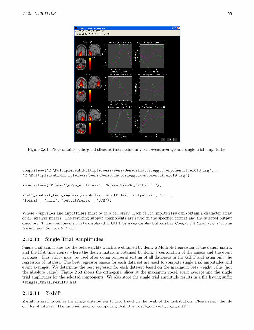
2.12. UTILITIES 55
Figure 2.63: Plot contains orthogonal slices at the maximum voxel, event average and single trial amplitudes.
compFiles={’E:\Multiple_sub_Multiple_sess\sens\Sensorimotor_agg__component_ica_018.img’,...
’E:\Multiple_sub_Multiple_sess\sens\Sensorimotor_agg__component_ica_019.img’};
inputFiles={’F:\smr1\swSm_nifti.nii’, ’F:\smr2\swSm_nifti.nii’};
icatb_spatial_temp_regress(compFiles, inputFiles, ’outputDir’, ’.’,...
’format’, ’.nii’, ’outputPrefix’, ’STR’);
Where compFiles and inputFiles must be in a cell array. Each cell in inputFiles can contain a character arrayof 3D analyze images. The resulting subject components are saved in the specified format and the selected outputdirectory. These components can be displayed in GIFT by using display buttons like Component Explore, OrthogonalViewer and Composite Viewer.
2.12.13 Single Trial Amplitudes
Single trial amplitudes are the beta weights which are obtained by doing a Multiple Regression of the design matrixand the ICA time course where the design matrix is obtained by doing a convolution of the onsets and the eventaverages. This utility must be used after doing temporal sorting of all data-sets in the GIFT and using only theregressors of interest. The best regressor onsets for each data set are used to compute single trial amplitudes andevent averages. We determine the best regressor for each data-set based on the maximum beta weight value (notthe absolute value). Figure 2.63 shows the orthogonal slices at the maximum voxel, event average and the singletrial amplitudes for the selected components. We also store the single trial amplitude results in a file having suffix*single_trial_results.mat.
2.12.14 Z-shift
Z-shift is used to center the image distribution to zero based on the peak of the distribution. Please select the fileor files of interest. The function used for computing Z-shift is icatb_convert_to_z_shift.
56 CHAPTER 2. GETTING STARTED WITH GIFT
2.12.15 Percent Variance
Percent variance utility can be used after running a group ICA analysis. Percent variance explained by the componentsin the data is calculated by doing a Multiple Regression of the BOLD signal and the component time courses ateach voxel where the component time courses are treated as a model. After the calculation is done, the final resultis printed to the MATLAB command window.
2.13 More Information
2.13.1 Batch Script
Analysis
Batch script is an alternative way to run the group ICA. Input_data_subjects_1.m and Input_data_subjects_2.m
are provided as examples. The function for running the batch file is icatb_batch_file_run. The syntax for thefunction is as given below:
Type icatb_batch_file_run(inputFile) at the MATLAB command prompt.
Where inputFile is the full file path for the input data of the
subjects.
Batch script and input data files are located in folder icatb_batch_files. Parameters in the input file are as follows:
• perfType - Group PCA performance settings. The best match for each option is dependent on the variableMAX_AVAILABLE_RAM in defaults file. Options are 1, 2 and 3.
– 1 - Maximize performance.
– 2 - Use less memory.
– 3 - User specified settings will be selected based on the PCA options.
• which_analysis - Options are 1 and 2. If you select 2, group ICA is run using ICASSSO. The following arethe options available:
– icasso_opts.sel_mode - Selection mode. Options are ”randinit”, ”bootstrap” and ”both”.
– icasso_opts.num_ica_runs - Number of times you want ICA to be run.
• dataSelectionMethod - There are four ways to select the data and the SPM design matrix (required fortemporal sorting). Options are 1, 2, 3 and 4. Each option is explained below:
– 1 - Data will be selected automatically if you specify the root folder for subjects and sessions, file pattern, aflag and file numbers to include. Options for flag are data_in_subject_folder and data_in_subject_subfolder.
∗ data_in_subject_subfolder - Data is selected from the subject sub-folders. Number of sessions isequal to the number of sub-folders containing the specified file pattern.
∗ data_in_subject_folder - Data is selected from the subject folders. The number of sessions is 1 andthe number of subjects is equal to the number of subject folders containing the specified file pattern.
spmDesignFilter - Specify design matrix filter pattern here if you have selected diff_sub_diff_sess
option for variable keyword_designMatrix. It looks for the design matrix in the respective subject folderor session folders.
– 2 - This option can be used when all the data is not in one directory. You need to specify the data directoryfor each subject and session followed by file pattern. The required variables are selectedSubjects andnumOfSess. selectedSubjects contains the names (arbitrary) of subjects (s1 refers to subject1, s2 refersto subject 2, etc) and numOfSess contains the number of sessions. Subject 1 session 1 data informationmust be entered in variable s1_s1 and subject 2 session 2 information must be entered in variable s1_s2.Design matrix information must be entered in _designMat variable.
– 3 - This option uses regular expressions to get the data set directories. The required variables are asfollows:
∗ input_directory_name - Full path of the directory where the subjects and sessions are located.

2.13. MORE INFORMATION 57
∗ subject_dir_regexp - Regular expression used for matching subject directories. This variable acceptsnested paths. For example, to match single slice data in the example subjects directory, you can useSub\w+; single\w+ regular expression where semi-colon is used as a delimiter. If there are no subjectdirectories inside the input directory, leave it as empty.
∗ session_dir_regexp - Regular expression used for getting the session directories inside the subjectdirectories. Unlike subject_dir_regexp variable this cannot contain nested paths. If there are nosession directories, leave this as empty.
Note: More information on regular expressions is given in the Appendix 4.5. For a detailed informa-tion about regular expressions, please refer to the MATLAB help.
∗ data_file_pattern - File pattern used for getting data. Use wild card not regular expressions.
∗ file_numbers_to_include - This option will let you work on a subset of files. Enter the file numbersto include. Leave it as empty if you want to include all the files.
∗ spm_stats_dir - SPM stats directory name relative to subject or session directories. GIFT will auto-matically search in the appropriate directories to get SPM.mat file for the subject. Please note that thisvariable will be read only when you use diff_sub_diff_sess value for the variable keyword_designMatrix.
– 4 - This option is useful when you want to specify the file names directly. Each variable is explained below:
∗ input_data_file_patterns - File patterns in a cell of dimensions equal to number of subjects andsessions. Each new subject must be entered in a new row.
∗ input_design_matrices - This variable will be read only when you are using a different designbetween subjects and sessions.
∗ dummy_scans - Enter number of dummy scans to exclude from the analysis.
• keyword_designMatrix - Design matrix is used for sorting the components temporally during display and willnot be used during the analysis stage except for semi-blind ICA. There are four options like no, same_sub_same_sess,same_sub_diff_sess and diff_sub_diff_sess.
– no - SPM design matrix is not specified for the analysis.
– same_sub_same_sess - All the subjects and sessions will share the same regressors. Specify location ofthe SPM design matrix in variable OnedesignMat.
– same_sub_diff_sess - Different regressors can be specified over sessions but same over subjects. Specifylocation of the SPM design matrix in variable OnedesignMat.
– diff_sub_diff_sess - Different regressors can be specified over subjects and sessions.
• outputDir - Output directory of the analysis.
• prefix - All the output files will be pre-pended with this prefix.
• maskFile - Specify the location of the mask file or leave it as empty (Default mask).
• preproc_type - Specify type of data pre-processing.
– 1 - Remove mean per time point
– 2 - Remove mean per voxel
– 3 - Intensity normalization
– 4 - Variance normalization
• group_pca_type - Select the type of group PCA.
– ’subject specific’ - Subject specific
– ’grand mean’ - Grand mean
• pcaType - Specify PCA type.
– 1 - Standard

58 CHAPTER 2. GETTING STARTED WITH GIFT
– 2 - Expectation Maximization
– 3 - SVD
• pca_opts - Optional parameters for PCA.
– Standard PCA:
∗ pca_opts.stack_data - Options are as follows:
· ’Yes’ - Data sets are stacked to compute covariance matrix. This option assumes that there isenough RAM to stack the data sets and for computing the covariance matrix. Full storage ofcovariance matrix is used.
· ’No’ - A pair of data sets are loaded at a time to compute covariance matrix. This option usesless memory usage but slower than the other option. You also have the option to store only thelower triangular portion of the covariance matrix (packed storage) when using this option.
∗ pca_opts.storage - Options are ’Full’ and ’Packed’. Packed storage scheme uses only lower triangularportion of symmetric matrix to compute eigen values.
∗ pca_opts.precision - Options are ’Double’ and ’Single’. Single precision is accurate up to 7 digitsafter decimal place and uses 50% less memory usage when compared to double precision.
∗ pca_opts.eig_solver - Options are ’Selective’ and ’All’. These options will be used only when youuse packed storage scheme. Use option ’All’ only when there are convergence issues with the option’Selective’.
– Expectation Maximization:
∗ pca_opts.stack_data - Options are as follows:
· ’Yes’ - This option assumes that there is enough RAM to stack the data sets.
· ’No’ - A data-set is loaded at a time to compute the transformation matrix.
∗ pca_opts.precision - Options are ’Double’ and ’Single’.
∗ pca_opts.tolerance - Enter stopping tolerance. Default is 1e-4.
∗ pca_opts.max_iter - Enter maximum number of iterations to use.
– SVD:
∗ pca_opts.precision - Options are ’Double’ and ’Single’.
∗ pca_opts.solver - Options are ’Selective’ and ’All’.
• backReconType - Options are 1, 2, 3 and 4.
– 1 - Regular
– 2 - Spatial-temporal regression
– 3 - GICA3
– 4 - GICA
• numReductionSteps - The number of reduction steps used and is dependent on the number of data-sets used.A maximum of three reduction steps is used.
• doEstimation - 1 means dimensionality estimation is done and PC step numbers are set to this value. Youcould select max, mean or median for a particular PC step in variable estimation_opts.
• numOfPC1 - Number of PC for reduction step 1.
• numOfPC2 - Number of PC for reduction step 2.
• numOfPC3 - Number of PC for reduction step 3.
• scaleType - Options are 0, 1, 2, 3 and 4.
– 0 - No scaling
– 1 - Scale components to percent signal change
– 2 - z-scores
2.13. MORE INFORMATION 59
– 3 - Scaling in timecourses
– 4 - Scaling in maps and timecourses
• algoType - Currently there are 16 ICA/IVA algorithms available in the GIFT toolbox. The algorithms are asfollows:
– 1 - Infomax
– 2 - FastICA
– 3 - ERICA
– 4 - SIMBEC
– 5 - EVD
– 6 - JADE OPAC
– 7 - AMUSE
– 8 - SDD ICA
– 9 - Semi-blind ICA
– 10 - Constrained ICA (Spatial)
– 11 - Radical ICA
– 12 - Combi
– 13 - ICA-EBM
– 14 - FBSS
– 15 - IVA-GL
– 16 - MOO-ICAR
• refFunNames - Reference function or regressor names to constrain ICA time courses. This is needed when usingsemi-blind ICA for the analysis.
• refFiles - Spatial reference or template files required to constrain the ICA source maps. This variable isrequired when Constrained ICA (Spatial) and MOO-ICAR algorithms are used for doing ICA. Enter the filesin a cell array.
Display
Display methods like Component Explorer, Composite Viewer and Orthogonal Viewer can be accessed through abatch script. The function for running the batch file is icatb_batch_display. The syntax for the function is asgiven below:
Type icatb_batch_display(inputFile) at the MATLAB command prompt
Where inputFile is the file containing the necessary display
parameters.
The display parameters in the input file are as follows:
• sourceDir - Directory where fMRI images are located.
• sourceFilePattern - File pattern for fMRI images.
• outputDir - Directory where the component images are located.
• compNumbers - Component numbers to plot.
• structFile - All the component images will be overlaid on this anatomical file.
• returnValue - Variable used for plotting activations or deactivations or activations and deactivations on spatialmap. There are four options like 1, 2, 3 and 4.
– 1 - Positive and Negative
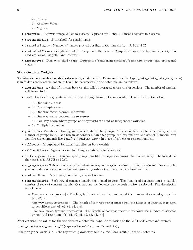
60 CHAPTER 2. GETTING STARTED WITH GIFT
– 2 - Positive
– 3 - Absolute Value
– 4 - Negative
• convertToZ - Convert image values to z-scores. Options are 1 and 0. 1 means convert to z-scores.
• thresholdValue - Z-threshold for spatial maps.
• imagesPerFigure - Number of images plotted per figure. Options are 1, 4, 9, 16 and 25.
• anatomicalPlane - Slice plane used for Component Explorer or Composite Viewer display methods. Optionsused are ’axial’, ’sagittal’ and ’coronal’.
• displayType - Display method to use. Options are ’component explorer’, ’composite viewer’ and ’orthogonalviewer’.
Stats On Beta Weights
Statistics on beta weights can also be done using a batch script. Example batch file (Input_data_stats_beta_weights.m)is in folder icatb/icatb_batch_files. The parameters in the batch file are as follows:
• averageRuns - A value of 1 means beta weights will be averaged across runs or sessions. The number of sessionswill be set to 1.
• desCriteria - Design criteria used to test the significance of components. There are six options like:
– 1 - One sample t-test
– 2 - Two sample t-test
– 3 - One way anova between the groups
– 4 - One way anova between the regressors
– 5 - Two way anova where groups and regressors are used as independent variables
– 6 - Multiple Regression
• groupInfo - Variable containing information about the groups. This variable must be a cell array of sizenumber of groups by 3. Each row must contain a name for group, subject numbers and session numbers. Youcan also use commands like load(’c:\healthy.asc’) in place of subject or session numbers.
• selGroups - Groups used for doing statistics on beta weights.
• selConditions - Regressors used for doing statistics on beta weights.
• multi_regress_files - You can specify regressor files like age, test scores, etc in a cell array. The format forthe text files is ASCII or MAT.
• eq_regressors - This option is provided when one way anova (groups) design criteria is selected. For example,you could do a one way anova between groups by subtracting one condition from another.
• contrastNames - A cell array containing contrast names.
• contrastMatrix - Each row of contrast matrix must equal to zero. The number of contrasts must equal thenumber of rows of contrast matrix. Contrast matrix depends on the design criteria selected. The descriptionis as follows:
– One way anova (groups) - The length of contrast vector must equal the number of selected groups like[g1, g2, etc].
– One way anova (regressors) - The length of contrast vector must equal the number of selected regressorsor conditions like [c1, c2, c3, c4, etc].
– Two way anova (groups, regressors) - The length of contrast vector must equal the number of selectedgroups and regressors like [g1, g2, c1, c2, c3, c4, etc].
After entering the values for the variables in a batch file, type the following at the MATLAB command prompt:
icatb_statistical_testing_TC(regressParamFile, userInputFile);
Where regressParamFile is the regression parameters text file and userInputFile is the batch file.

2.13. MORE INFORMATION 61
Mancova
Batch template for mancova is located at icatb\icatb_batch_files\input_mancovan.m. The following are thevariables:
• outputDir - Output directory to place the analysis results.
• ica_param_file - Full path to ICA parameter file.
• features - Options are spatial maps, timecourses spectra and FNC correlations.
• covariates - Enter covariates information in a cell array of dimensions no. of covariates by 4. The fourcolumns are covariate name, type, vector and transformation function. You could use file name instead ofentering covariate vector. This file must be ascii for continuous covariates and a text file with new line,comma or tab as delimiter for categtorical covariates. Transformation function will be used only for continuouscovariates.
• interactions - Specify pairwise model interactions. If you don’t want to use interactions, you could leave itas empty.
• comp_network_names - Component networks. Use name by values where values are component numbers. Thenames information will be used in future release for advanced plotting.
• numOfPCs - Number of principal components used to reduce the data in voxel or spectra dimension which willbe used in multi-variate tests. The vector length must match the no. of features.
• p_threshold - Significance threshold used in multivariate and univariate tests.
• TR - TR of the experiment in seconds.
After entering the parameters, use icatb_mancovan_batch(inputFile); at the command prompt.
Stats On Individual Subject Component Maps
You can test the significance of components by doing a one sample t-test or two sample t-test on images. We nowprovide an option in GIFT to do one sample t-test or two sample t-test on images using SPM5.
• One sample t-test - One sample t-test for each component will be automatically calculated if you set variableSPM_STATS_WRITE_TAL in icatb_defaults.m to 1 or 2. If you set variable SPM_STATS_WRITE_TAL value to 1only one sample t-test will be calculated whereas a value of 2 will also write talairach tables for the t-map.
Note: An option is also provided in ”Utilities” (Figure 2.1) drop down box to calculate t-maps for the selecteddata-sets.
• Two sample t-test - When you click ”Utilities” (Figure 2.1) drop down box and have selected ”SPM Stats” asthe option, a figure window will open to select the design criteria. When you select design as ”Two sample t-test”, two sample t-test for a component will be calculated between the selected groups by using a explicit mask.The explicit mask is calculated by applying a threshold (SPM_STATS_TTEST_THRESHOLD) on t-map obtained bydoing a one sample t-test on data-sets.
Note: When you set SPM_STATS_TTEST2_EXPLICIT_MASK variable in icatb_defaults.m file to 0, explicit maskis not used.
2.13.2 Output Files Naming
• Parameter file - File used for storing parameters before and after the analysis. _ica_parameter_info.mat isthe suffix used for parameter file.
• Reduction step file - After PCA, the information is stored in a MAT file. _pca_r is the suffix used for reductionfiles.
• ICA step file - After ICA, the information is stored in a MAT file with the suffix _ica. The aggregate imagesare written in Analyze or Nifti format with the suffix _agg__component_ica_.

62 CHAPTER 2. GETTING STARTED WITH GIFT
Figure 2.64: Source Based Morphometry
• Back reconstruction step file - After back reconstruction step, the information is stored in a MAT file with thesuffix _ica_br.
• Calibrate step file - After scaling, the information is stored in a MAT file with the suffix _ica_c.
• Component map file - Component maps are stored with the suffix _component_ica_ in Analyze or Nifti format.
• Component time course file - Component time course for a particular data-set is stored with the suffix_timecourses_ica_ in Analyze or Nifti format.
Note: To load the image files, use icatb_loadData(file_name).
2.14 Source Based Morphometry
Source Based Morphometry (SBM) is a multivariate tool to study the gray matter differences between the patientsand controls ([1] and [22]). ICA is used on the subject images to determine the maximally independent sources.Basically ICA decomposes data into subject loading coefficients and component maps. It is similar to doing singlesubject single session analysis in the GIFT except the timepoints are subject images. To invoke SBM (Figure 2.64),type sbm or groupica smri at the MATLAB command prompt. The following are the differences between the GIFTand SBM:
• Setup ICA - Default mask used in the SBM includes voxels greater than or equal to 1% of mean of the data.
• Display - Subject explorer is excluded in the display GUI.
• Output files naming - Component maps are stored with the suffix *group*component*ica* in Analyze or Niftiformat. Subject component loading coefficients are stored with the suffix *group*loading*coeff* in Analyzeor Nifti format. To load the image files, use icatb_loadData(file_name).
• Batch template is provided in icatb\icatb_batch_files\Input_sbm.m. Specify modalityType as ’smri’ andenter the parameters similar to one subject one session analysis as in the GIFT. After entering the parameters,use icatb_batch_file_run(inputFile) at the MATLAB command prompt.
• Only remove components, write talairach tables and ICASSO utilities are included.
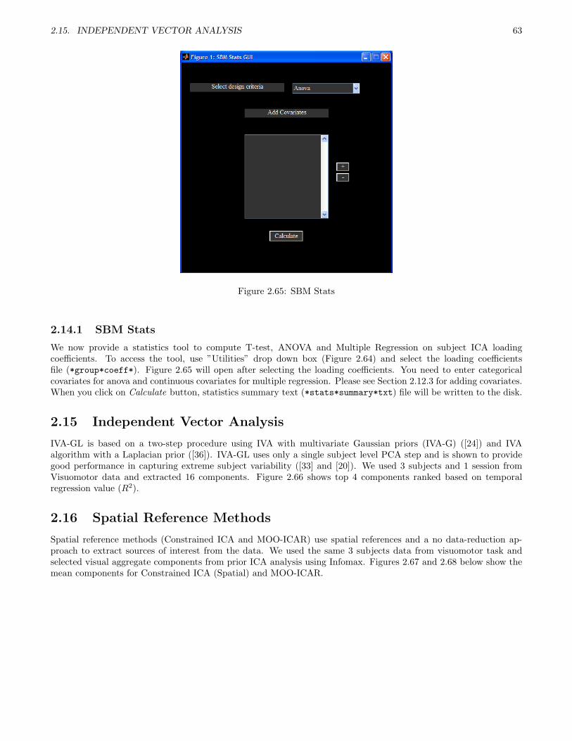
2.15. INDEPENDENT VECTOR ANALYSIS 63
Figure 2.65: SBM Stats
2.14.1 SBM Stats
We now provide a statistics tool to compute T-test, ANOVA and Multiple Regression on subject ICA loadingcoefficients. To access the tool, use ”Utilities” drop down box (Figure 2.64) and select the loading coefficientsfile (*group*coeff*). Figure 2.65 will open after selecting the loading coefficients. You need to enter categoricalcovariates for anova and continuous covariates for multiple regression. Please see Section 2.12.3 for adding covariates.When you click on Calculate button, statistics summary text (*stats*summary*txt) file will be written to the disk.
2.15 Independent Vector Analysis
IVA-GL is based on a two-step procedure using IVA with multivariate Gaussian priors (IVA-G) ([24]) and IVAalgorithm with a Laplacian prior ([36]). IVA-GL uses only a single subject level PCA step and is shown to providegood performance in capturing extreme subject variability ([33] and [20]). We used 3 subjects and 1 session fromVisuomotor data and extracted 16 components. Figure 2.66 shows top 4 components ranked based on temporalregression value (R2).
2.16 Spatial Reference Methods
Spatial reference methods (Constrained ICA and MOO-ICAR) use spatial references and a no data-reduction ap-proach to extract sources of interest from the data. We used the same 3 subjects data from visuomotor task andselected visual aggregate components from prior ICA analysis using Infomax. Figures 2.67 and 2.68 below show themean components for Constrained ICA (Spatial) and MOO-ICAR.

64 CHAPTER 2. GETTING STARTED WITH GIFT
80 76 72 68 64 60 56
52 48 44 40 36 32 28
24 20 16 12 8 4 0
−4 −8 −12 −16 −20 −24 −28
−32 −36 −40 −44 −48 −52
RL
0
8.7
−1012
Scans
Component 6 temporal multiple regression = 0.79418
80 76 72 68 64 60 56
52 48 44 40 36 32 28
24 20 16 12 8 4 0
−4 −8 −12 −16 −20 −24 −28
−32 −36 −40 −44 −48 −52
RL
0
8.5
−2
0
2
Scans
Component 7 temporal multiple regression = 0.49603
80 76 72 68 64 60 56
52 48 44 40 36 32 28
24 20 16 12 8 4 0
−4 −8 −12 −16 −20 −24 −28
−32 −36 −40 −44 −48 −52
RL
0
6.6
−202
Scans
Component 9 temporal multiple regression = 0.23328
80 76 72 68 64 60 56
52 48 44 40 36 32 28
24 20 16 12 8 4 0
−4 −8 −12 −16 −20 −24 −28
−32 −36 −40 −44 −48 −52
RL
0
9.2
−202
Scans
Component 8 temporal multiple regression = 0.2197
Figure 2.66: IVA Results
80 76 72 68 64 60 56
52 48 44 40 36 32 28
24 20 16 12 8 4 0
−4 −8 −12 −16 −20 −24 −28
−32 −36 −40 −44 −48 −52
RL
0
9.9
−1012
Scans
Component 1 Not Sorted
80 76 72 68 64 60 56
52 48 44 40 36 32 28
24 20 16 12 8 4 0
−4 −8 −12 −16 −20 −24 −28
−32 −36 −40 −44 −48 −52
RL
0
10.6
−101
Scans
Component 2 Not Sorted
Figure 2.67: Constrained ICA Results
80 76 72 68 64 60 56
52 48 44 40 36 32 28
24 20 16 12 8 4 0
−4 −8 −12 −16 −20 −24 −28
−32 −36 −40 −44 −48 −52
RL
0
10.8
−1012
Scans
Component 1 Not Sorted
80 76 72 68 64 60 56
52 48 44 40 36 32 28
24 20 16 12 8 4 0
−4 −8 −12 −16 −20 −24 −28
−32 −36 −40 −44 −48 −52
RL
0
11.3
−101
Scans
Component 2 Not Sorted
Figure 2.68: MOO-ICAR Results

Chapter 3
Process involved in Group ICA
In this chapter, the process involved in group ICA is described. This chapter is divided into four sections. Eachsection is a step involved in group ICA. In Section 3.1, data reduction step is discussed. In Section 3.2, ICA processand the different ICA algorithms used in GIFT are explained. In Section 3.4, calibrating the components imagesand time-courses is discussed. Chapter 3.5 is used to describe the statistics involved in the toolbox.
3.1 Data Reduction
Data reduction is a step to reduce the size of the subject’s functional data. Principal Components Analysis (PCA) isused as a technique to reduce the dimensions. A single subject might be reduced from 53*63*34*220 to 53*63*34*50.Two or three data reduction steps are used for multiple subjects (See Table 2.1).
• Two data reduction steps - After each subject’s functional data is reduced, the subjects are then concatenatedinto one group and put through another data reduction step. Figure 3.1 shows three data-sets passed throughtwo data reduction steps.
• Three data reduction steps - After each subject’s functional data is reduced, the subjects are then concatenatedinto groups and put through another data reduction step. The number of subjects to put into each group iscalled partitions. The number of partitions is equal to one-fourth of the number of data-sets selected. Reduceddata from the groups are stacked into one group and put through the final data reduction.
Note: Two data reduction steps is the recommended approach for group PCA.
The next stage is applying ICA on this reduced data-set.
3.2 Independent Component Analysis
Independent Component Analysis (ICA) is used to find independent components (ICs, Figure 3.2). GIFT includesa number of ICA algorithms that are available online and on ICALAB ([9]). Here we briefly introduce some of theICA algorithms included in GIFT and cite relevant references. We also discuss a few parameters that affect theirseparation performance and some of the observations we obtained in our runs with simulated and real fMRI data([27]) using Infomax, FastICA, Jade, SIMBEC and AMUSE.
Figure 3.1: First each data-set is reduced using PCA where R term indicates reduced data. These three reduceddata-sets are concatenated into one group (or partitions). The grouped data is passed through another data-reductionstep.
65

66 CHAPTER 3. PROCESS INVOLVED IN GROUP ICA
Figure 3.2: Reduced data-set from the last step in the data-reduction stage is used and ICA algorithm is applied.The components represent group and not of individual subjects. The next stage is Back-Reconstruction.
3.2.1 Infomax
Infomax ([3]) maximizes the information transfer from the input to the output of a network using a non-linearfunction. A majority of applications of ICA to fMRI use Infomax since the sources of interest in this case are supergaussian in nature and the algorithm favors separation of super-gaussian sources. However, the artifacts presentin fMRI data typically have sub-gaussian distributions. To improve separation of the mixture containing bothsuper-gaussian and sub-gaussian sources, Extended Infomax ([37]) can be used.To use Extended Infomax, choose ’1’ instead of the default of ’0’ while selecting ICA options for the Infomaxalgorithm. Based on our experiments, we observed that Infomax is a reliable choice for performing ICA on fMRIdata. Z-scores for Infomax were higher than the other algorithms for the task-related source, indicating that Infomaxachieves a higher contrast to noise ratio. Repeated runs showed that the changing initial random condition does notchange results significantly. Infomax is much slower than the other algorithms listed in the toolbox.
3.2.2 Fast ICA
FastICA ([7]) maximizes the higher order statistics or negentropy of the output to maximize the non-gaussianity ofthe estimated sources using fixed point iterations. Two approaches exist: The symmetric approach estimates all theICs in parallel and the deflationary approach estimates the ICs one at a time. The tanh, pow3, gauss and skew nonlinearities can be used ([8]).The desired non-linearity can be chosen while selecting ICA options for FastICA. In our experiments, we usedFastICA in the symmetric mode and compared results obtained using the non linearities tanh, pow3 and gauss. Onsimulated data, this algorithm does better in terms of spatial correlation of the estimated sources with the originalsources, for super-gaussian sources when compared to the other sources. For smaller number of components (numberof components=5), FastICA with the gauss non-linearity provides better performance compared to the other twonon-linearities for the gaussian and sub-gaussian sources. However, for a slightly larger simulated set (number ofcomponents=8), all three non-linearities result in very similar performance. Overall, the general performance ofFastICA using tanh is better than the results obtained using the other two non-linearities. For actual fMRI data, weobserved that for the transiently task-related component the spatial extent is slightly higher in FastICA as comparedto Infomax. FastICA is slow when it has convergence problems and in this case it would be advisable to use thestabilized version of the algorithm. This can be done by changing the stabilization option to ’ON’, while selectingthe ICA options.
3.2.3 JADE OPAC
JADE (joint approximate diagonalization of eigenmatrices) ([19]), uses the Jacobi technique, to perform joint ap-proximate diagonalization on fourth order cumulant matrices to achieve spatial independence among the sources.The version of JADE included in GIFT is MATLAB optimized with a reduced number of eigen matrices ([9]).JADE is fast and the results are comparable to those obtained using Infomax. In the case of transiently task relatedcomponents this algorithm shows spatial extent of activations to be higher than the obtained using Infomax.
3.2.4 SIMBEC
SIMBEC (simultaneous blind extraction using cumulants) ([32]), uses natural gradient ascent in a Stiefel manifoldto simultaneously extract sources using a contrast function based on higher order cumulants with a learning ratethat provides fast convergence.In our simulations, we observed that for smaller number of components, SIMBEC performs well for the sources ofinterest. However, SIMBEC may prove useful to identify the sub-gaussian sources, i.e. artifacts in fMRI data as its
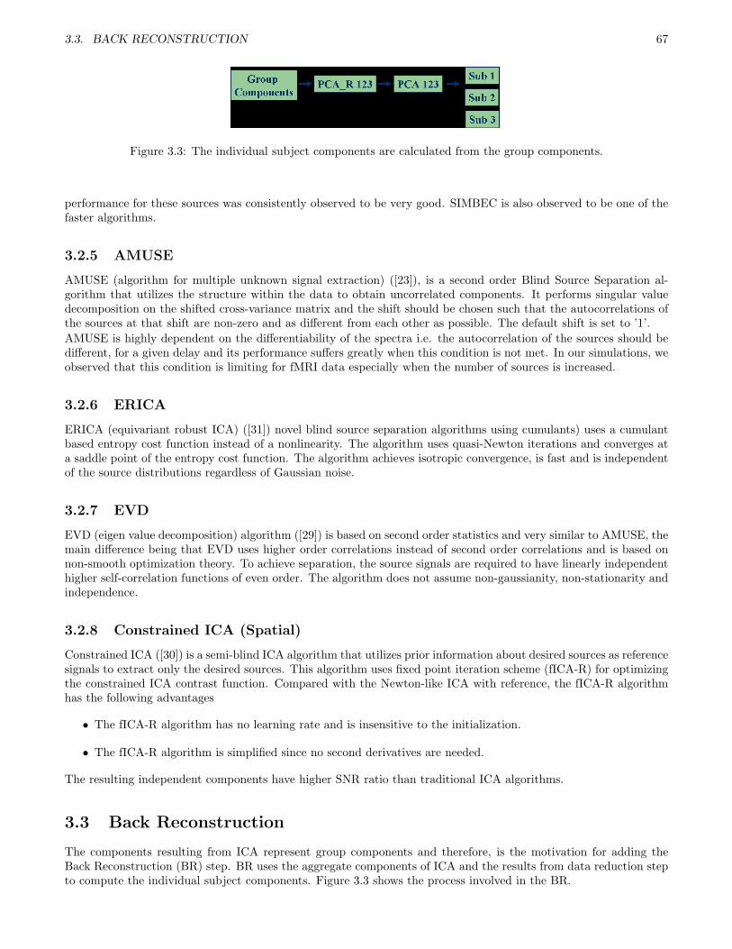
3.3. BACK RECONSTRUCTION 67
Figure 3.3: The individual subject components are calculated from the group components.
performance for these sources was consistently observed to be very good. SIMBEC is also observed to be one of thefaster algorithms.
3.2.5 AMUSE
AMUSE (algorithm for multiple unknown signal extraction) ([23]), is a second order Blind Source Separation al-gorithm that utilizes the structure within the data to obtain uncorrelated components. It performs singular valuedecomposition on the shifted cross-variance matrix and the shift should be chosen such that the autocorrelations ofthe sources at that shift are non-zero and as different from each other as possible. The default shift is set to ’1’.
AMUSE is highly dependent on the differentiability of the spectra i.e. the autocorrelation of the sources should bedifferent, for a given delay and its performance suffers greatly when this condition is not met. In our simulations, weobserved that this condition is limiting for fMRI data especially when the number of sources is increased.
3.2.6 ERICA
ERICA (equivariant robust ICA) ([31]) novel blind source separation algorithms using cumulants) uses a cumulantbased entropy cost function instead of a nonlinearity. The algorithm uses quasi-Newton iterations and converges ata saddle point of the entropy cost function. The algorithm achieves isotropic convergence, is fast and is independentof the source distributions regardless of Gaussian noise.
3.2.7 EVD
EVD (eigen value decomposition) algorithm ([29]) is based on second order statistics and very similar to AMUSE, themain difference being that EVD uses higher order correlations instead of second order correlations and is based onnon-smooth optimization theory. To achieve separation, the source signals are required to have linearly independenthigher self-correlation functions of even order. The algorithm does not assume non-gaussianity, non-stationarity andindependence.
3.2.8 Constrained ICA (Spatial)
Constrained ICA ([30]) is a semi-blind ICA algorithm that utilizes prior information about desired sources as referencesignals to extract only the desired sources. This algorithm uses fixed point iteration scheme (fICA-R) for optimizingthe constrained ICA contrast function. Compared with the Newton-like ICA with reference, the fICA-R algorithmhas the following advantages
• The fICA-R algorithm has no learning rate and is insensitive to the initialization.
• The fICA-R algorithm is simplified since no second derivatives are needed.
The resulting independent components have higher SNR ratio than traditional ICA algorithms.
3.3 Back Reconstruction
The components resulting from ICA represent group components and therefore, is the motivation for adding theBack Reconstruction (BR) step. BR uses the aggregate components of ICA and the results from data reduction stepto compute the individual subject components. Figure 3.3 shows the process involved in the BR.

68 CHAPTER 3. PROCESS INVOLVED IN GROUP ICA
Figure 3.4: The individual subject components are calibrated to percent signal change using the original fMRI dataas reference.
Figure 3.5: Mean, standard deviation and t-maps are calculated for each component over the data-sets used.
3.4 Scaling Components
The spatial maps and time courses of components have arbitrary units after the back reconstruction step. Componentspatial maps and timecourses can be scaled using percent signal change, z-scores, scaling in timecourses or scalingin timecourses and maps. Figure 3.4 shows the spatial maps and timecourses scaled to percent signal change.
3.5 Group Stats
Statistics is performed on the group of subjects. Mean, standard deviation and t-maps are calculated on the group ofsubjects. To give an illustration, let us say M data-sets are used and N components are extracted for each data-set.The mean, standard deviation and t-map are calculated for each component (Figure 3.5) over the number of data-setsused. This will produce N components for mean, standard deviation and t-map.
Bibliography
[1] A. Caprihan, C. Abbott, J. Yamamoto, G. D. Pearlson, N. Bizzozero, J. Sui, and V. D. Calhoun, ”Source-basedmorphometry analysis of group differences in fractional anisotropy in schizophrenia,” Brain Connectivity, InPress
[2] http://afni.nimh.nih.gov/afni
[3] A. J. Bell and T. J. Sejnowski, ”An information maximisation approach to blind separation and blind deconvo-lution,” Neural Comput., vol. 7, pp. 1129-1159, 1995.
[4] A. R. Franco, A. Pritchard, V. D. Calhoun, A. R Mayer, ”Inter-rater and Inter-method Reliability for Selectingthe Default Mode Network during Data-Driven Analyses”, HBM, vol. 30, pp. 2293-2303, 2009.
[5] A. Garrity, G. D. Pearlson, K. McKiernan, D. Lloyd, K. A. Kiehl, and V. D. Calhoun, ”Aberrant default modefunctional connectivity in schizophrenia” Am.J.Psychiatry, vol. 164, pp. 450-457, 2007.
[6] GLASSO, http://cran.r-project.org/web/packages/glasso/.
[7] A. Hyvarinen and E. Oja, ”A fast fixed-point algorithm for independent component analysis,” Neural Comput.,vol. 9, no. 7, pp. 1483-1492, 1997.
[8] A. Hyvarinen, ”Fast and robust fixed-point algorithms for independent component analysis,” Neural Networks,vol. 10, pp. 626-634, 1999.
[9] A. Cichocki, S. Amari, K. Siwek, T. Tanaka et al., ”ICALAB Toolboxes,”http://www.bsp.brain.riken.jp/ICALAB.
[10] Chronux, http://chronux.org
[11] D. Glahn, SPM fMRI Analysis, 2000.
[12] EEGLAB Toolbox, http://sccn.ucsd.edu/eeglab/
[13] E. Allen, E. Damaraju, S. M. Plis, E. Erhardt, T. Eichele, and V. D.Calhoun, ”Tracking whole-brain connectivitydynamics in the resting state”, Cereb Cortex, in press.
[14] E. Allen, T. Eichele, L. Wu, and V. D. Calhoun, ”EEG Signatures of Functional Connectivity States,” in HumanBrain Mapping, Seattle, WA, 2013
[15] E. Allen, E. Erhardt, E. Damaraju, W. Gruner, J. Segall, R. Silva, M. Havlicek, S. Rachakonda, J. Fries, R.Kalyanam, A. Michael, J. Turner, T. Eichele, S. Adelsheim, A. Bryan, J. R. Bustillo, V. P. Clark, S. Feldstein,F. M. Filbey, C. Ford, K. Hutchison, R. Jung, K. A. Kiehl, P. Kodituwakku, Y. Komesu, A. R. Mayer, G. D.Pearlson, J. Phillips, J. Sadek, M. Stevens, U. Teuscher, R. J. Thoma, and V. D. Calhoun, ”A baseline for themultivariate comparison of resting state networks,” Frontiers in Human Neuroscience, vol. 1, p. 12, 2011
[16] E. Allen, E. Erhardt, T. Eichele, A. R. Mayer, and V. D. Calhoun, ”Comparison of pre-normalization methodson the accuracy of group ICA results,” in Proc. HBM, Barcelona, Spain, 2010.
[17] E. Erhardt, S. Rachakonda, E. Bedrick, T. Adali, and V. D. Calhoun, ”Comparison of multi-subject ICAmethods for analysis of fMRI data,” in Proc. HBM, Barcelona, Spain, 2010.
[18] ICASSO Toolbox, http://www.cis.hut.fi/projects/ica/icasso/
69

70 BIBLIOGRAPHY
[19] J. F. Cardoso and A. Souloumiac, ”Blind beamforming for non gaussian signals,” IEE-Proc-F, vol. 140, no. 6,pp. 362-370,
[20] J. T. Dea, M. Anderson, E. Allen, V. D. Calhoun, and T. Adali ”IVA for multi- subject fMRI analysis: Acomparative study using a new simulation toolbox,” in Proc. IEEE Workshop on Machine Learning for SignalProcessing (MLSP), Beijing, China, Sep. 2011
[21] J. Knight, ”Signal Fraction Analysis and Artifact Removal in EEG”, Colorado State University, Fort Collins,Colorado, MS Thesis 2003.
[22] L. Xu, K. Groth, G. Pearlson, D. Schretlen, and V. Calhoun, ”Source Based Morphometry: The Use of Indepen-dent Component Analysis to Identify Gray Matter Differences with Application to Schizophrenia,” Hum BrainMapp, vol. 30, pp. 711-724, 2009.
[23] L. Tong, V. C. Soon, Y. F. Huang and R. Liu, ”Indeterminacy and identifiability of blind identification,” IEEETrans. Circuits Sys., vol. 38, pp. 499-509, 1991.
[24] M. Anderson, T. Adali and X.-L. Li, ”Joint Blind Source Separation of Multivariate Gaussian Sources: Algo-rithms and Performance Analysis,” IEEE Trans. Signal Process., 2012, 60, 1672-1683.
[25] M. J. McKneown, Scott Makeig, Greg G. Brown, Tzyy-Ping Jung, Sandra S. Kindermann, Anthony J. Bell andTerrence J. Sejnowski, ”Analysis of fMRI Data by Blind Separation Into Independent Spatial Components”,vol. 6, pp. 160-188, 1998.
[26] Melodic, http://www.fmrib.ox.ac.uk/fsl/melodic/index.html
[27] N. Correa, T. Adali, Yi-Ou Li and V. Calhoun, ”Comparison of Blind Source Separation algorithms for fMRIusing a new MATLAB toolbox: GIFT,” to be published in ICASSP 2005.
[28] N. Filippini, B. J. MacIntosh, M. G. Hough, G. M. Goodwin, G. B. Frisoni, S. M. Smith, P. M. Matthews, C.F. Beckmann, and C. E. Mackay, ”Distinct patterns of brain activity in young carriers of the APOE-epsilon4allele,” Proc Natl Acad Sci USA, vol. 106, pp. 7209-7214, Apr. 2009.
[29] P. Georgiev and A. Cichocki, ”Blind source separation via symmetric eigenvalue decomposition,” Proc. SixthInternational Symposium on Signal Processing and its Applications, Shangri-La Hotel, Kuala Lumpur, Malaysia,pp. 17-20, Aug. 2001.
[30] Q. Lin, J. Liu, Y. Zheng, H. Liang and V. D. Calhoun, ”Incorporating Spatial Hypotheses within ICA: AnEfficient Fixed-point ICA-R Algorithm Applied to fMRI Data”, Submitted to NeuroImage 2006.
[31] S. Cruces, L. Castedo, A. Cichochki, ”Novel blind source separation algorithms using cumulants, ” IEEE Inter-national Conference on Acoustics, Speech, and Signal Processing, vol. 5, pp. 3152-3155, Istanbul, Turkey, June2000.
[32] S. Cruces, A. Cichocki and S. Amari, “Criteria for the simultaneous blind extraction of arbitrary groups ofsources,” Int. Conf. Independent Component Analysis and Blind Sig. Separation, San Diego, California, USA,2001.
[33] S. Ma, R.Phlypo, V.D. Calhoun, and T. Adali ”Capturing group variability using IVA: A simulation study andgraph-theoretical analysis,” in Proc. IEEE Int. Conf. Acoust., Speech, Signal Processing (ICASSP), Vancouver,BC, Canada, May 2013.
[34] S.Roweis, ”EM algorithms for PCA and sensible PCA”, Advances in Neural Information Processing Systems.1998.
[35] Statistical Parameteric Mapping, http://www.fil.ion.ucl.ac.uk/spm/.
[36] T. Kim, H. T. Attias, S.-Y. Lee, and T.-W. Lee, ”Blind Source Separation Exploiting Higher-Order FrequencyDependencies,” IEEE Trans. Audio Speech Lang. Process., 2007, 15, 70-79.
[37] T. W. Lee, M. Girolami, and T. J. Sejnowski, ”Independent component analysis using an extended Infomaxalgorithm for mixed sub-Gaussian and super-Gaussian sources,” Neural Comput, vol. 11, no. 2, pp. 417-441,1999.

BIBLIOGRAPHY 71
[38] V.D. Calhoun, T. Adali, G.D. Pearlson, and J.J. Pekar, ”AMethod for Making Group Inferences From FunctionalMRI Data Using Independent Component Analysis”, HBM, vol. 14, pp. 140-151, 2001.
[39] V.D. Calhoun, T. Adali, J.J. Pekar, and G.D. Pearlson, ”Latency (in) Sensitive ICA: Group IndependentComponent Analysis of FMRI Data in the Temporal Frequency Domain”, NeuroImage, vol. 20, 2003. 1993.
[40] Y. Du, Y. Fan, ”Group information guided ICA for fMRI data analysis”, NeuroImage 69: 157-197 (2013).
[41] Y. Li, T. Adali, and V. D. Calhoun, ”Sample Dependence Correction For Order Selection In FMRI Analysis,”in Proc. ISBI, Washington, D.C., 2006.

72 BIBLIOGRAPHY
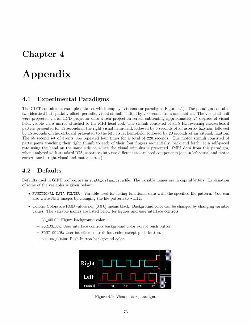
Chapter 4
Appendix
4.1 Experimental Paradigms
The GIFT contains an example data-set which employs visuomotor paradigm (Figure 4.1). The paradigm containstwo identical but spatially offset, periodic, visual stimuli, shifted by 20 seconds from one another. The visual stimuliwere projected via an LCD projector onto a rear-projection screen subtending approximately 25 degrees of visualfield, visible via a mirror attached to the MRI head coil. The stimuli consisted of an 8 Hz reversing checkerboardpattern presented for 15 seconds in the right visual hemi-field, followed by 5 seconds of an asterisk fixation, followedby 15 seconds of checkerboard presented to the left visual hemi-field, followed by 20 seconds of an asterisk fixation.The 55 second set of events was repeated four times for a total of 220 seconds. The motor stimuli consisted ofparticipants touching their right thumb to each of their four fingers sequentially, back and forth, at a self-pacedrate using the hand on the same side on which the visual stimulus is presented. fMRI data from this paradigm,when analyzed with standard ICA, separates into two different task-related components (one in left visual and motorcortex, one in right visual and motor cortex).
4.2 Defaults
Defaults used in GIFT toolbox are in icatb_defaults.m file. The variable names are in capital letters. Explanationof some of the variables is given below:
• FUNCTIONAL_DATA_FILTER - Variable used for listing functional data with the specified file pattern. You canalso write Nifti images by changing the file pattern to *.nii.
• Colors: Colors are RGB values i.e., [0 0 0] means black. Background color can be changed by changing variablevalues. The variable names are listed below for figures and user interface controls:
– BG_COLOR: Figure background color.
– BG2_COLOR: User interface controls background color except push button.
– FONT_COLOR: User interface controls font color except push button.
– BUTTON_COLOR: Push button background color.
Figure 4.1: Visuomotor paradigm.
73

74 CHAPTER 4. APPENDIX
– BUTTON_FONT_COLOR: Push button font color.
– Fonts for user interface controls:
∗ UI_FONTNAME: Font name.
∗ UI_FONTUNITS: Font units.
∗ UI_FS: Font size.
• Display Defaults: Defaults in display GUI are plotted first. These can be changed by accessing variables like:
– SORT_COMPONENTS: Options available are ’No’ to ’Yes’.
– IMAGE_VALUES: Options available are ’Positive’, ’Positive and Negative’, ’Absolute Value’ and ’Negative’.
– CONVERT_Z: Options are ’Yes’ and ’No’.
– THRESHOLD_VALUE: Threshold value to use voxels above or equal to the threshold
– IMAGES_PER_FIGURE: Options are ’1’, ’4’, ’9’, ’16’, ’25’.
– ANATOMICAL_PLANE: Options are ’axial’, ’sagittal’ and ’coronal’.
• DETRENDNUMBER: Detrend defaults for ICA time courses can be changed by changing the variable value. Optionsare 0, 1, 2 and 3.
• Smoothing parameters: When SMOOTHPARA variable is changed to ’Yes’ the time courses are smoothed by thevalue indicated in the variable SMOOTHINGVALUE.
• FLAG_ACKNOWLEDGE_CREATORS: Variable used to display acknowledgement for creators. You can turn off thedialog box by changing value to ’off’.
• ICAOPTIONS_WINDOW_DISPLAY: Variable used to display ICA options window. You can turn off the figurewindow by changing value to ’off’.
• STORE_DIRECTORY_INFORMATION: When this variable is changed to ’Yes’, directories specified in cell arrayDIRS_TO_BE_STORED are stored in the file selection window.
• ZIP_IMAGE_FILES: When this variable is set to ’Yes’, the component images will be compressed to a zip filebased on their viewing set.
• METHOD_ENTERING_REGRESSORS: Variable has three options like ’AUTOMATIC’, ’GUI’ and ’BATCH’ for tem-poral sorting. Each option is explained below:
– ’AUTOMATIC’ - Regressors in SPM.mat file will be used directly. For ’Different regressors over sessions’or ’Different regressors for subjects and sessions’ session related regressors will be used.
– ’GUI’ - Figure window will open to select regressors.
– ’BATCH’ - Regressors can be entered using a text file by specifying the file name. This is the best way toenter regressors if you have many data-sets and selected ’Different regressors over subjects and sessions’.
Note:
∗ TXTFILE_REGRESSORS is the variable used for specifying the sorting text file.
∗ Sorting text file specified in defaults will not be used if you had changed using Display GUI.
• FLIP_ANALYZE_IMAGES: Flip parameter for the analyze images. Default value is 0.
• NUM_RUNS_GICA: Number of times ICA will be run. Default is 1.
• DEFAULT_MASK_OPTION: Mask is calculated by doing a Boolean AND of voxels that surpass or equal the mean.By default first file for each subject is used. You can use all files by changing variable value to ’all files’.
• OPEN_DISPLAY_GUI: Option is provided to open the display GUI automatically after the analysis. You canturn off the option by changing variable value to 0.
• CENTER_IMAGES: A value of 1 means subject spatial maps will be centered based on the peak of the distribution.
• PREPROC_DEFAULT: Data pre-processing default.

4.2. DEFAULTS 75
Figure 4.2: Time course options.
– 1 - Remove mean per time point
– 2 - Remove mean per voxel
– 3 - Intensity normalization
– 4 - Variance normalization
• PCA_DEFAULT - PCA default.
– 1 - Standard
– 2 - Expectation Maximization
• BACKRECON_DEFAULT: Backreconstruction default.
– 1 - Regular
– 2 - Spatial-temporal Regression
– 3 - GICA3
– 4 - GICA
• SCALE_DEFAULT - Scaling components default.
– 0 - No scaling
– 1 - Scale To Original Data(%)
– 2 - Z-scores
– 3 - Scaling in Timecourses
– 4 - Scaling in Maps and Timecourses

76 CHAPTER 4. APPENDIX
Figure 4.3: Figure window used to select a directory, file or files.
4.3 Options Window
When you click ”Timecourse Options” sub menu in Options Menu (Figure 2.20), options window (Figure 4.2) appearswith the defaults used from the icatb_defaults.m. There are three categories in the left list box like Model Timecourse, ICA Time course” and Event Average. The explanation of each option in the list box is explained below:
• Model Time course:
– Normalize Model Timecourse: Model time course is normalized and the ICA time course is used as areference.
– Linear detrend Model Time course: Linear trend is removed in model time course.
• ICA Time course:
– Detrend Number: ICA time course is detrended with the number specified in popup control.
– Flip ICA Time course: ICA time course is flipped.
– Smoothing Parameter: ICA time course is smoothed if the option is set to ’Yes’.
– Smoothing Value: ICA time course is smoothed using the value specified in edit control.
• Event Average:
– Window size in seconds: Window size to display the event average of ICA time course.
– Interpolation factor: Factor to interpolate the ICA time course.
When you click OK button, the values in the controls are used and the time courses are plotted in the expandedview of time course (Figure 2.20). Cancel button closes the figure window. Default button uses the defaults fromicatb_defaults.m file.
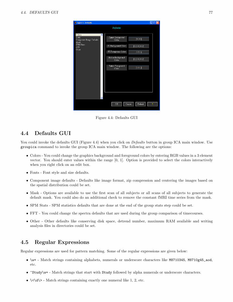
4.4. DEFAULTS GUI 77
Figure 4.4: Defaults GUI
4.4 Defaults GUI
You could invoke the defaults GUI (Figure 4.4) when you click on Defaults button in group ICA main window. Usegroupica command to invoke the group ICA main window. The following are the options:
• Colors - You could change the graphics background and foreground colors by entering RGB values in a 3 elementvector. You should enter values within the range [0, 1]. Option is provided to select the colors interactivelywhen you right click on an edit box.
• Fonts - Font style and size defaults.
• Component image defaults - Defaults like image format, zip compression and centering the images based onthe spatial distribution could be set.
• Mask - Options are available to use the first scan of all subjects or all scans of all subjects to generate thedefault mask. You could also do an additional check to remove the constant fMRI time series from the mask.
• SPM Stats - SPM statistics defaults that are done at the end of the group stats step could be set.
• FFT - You could change the spectra defaults that are used during the group comparison of timecourses.
• Other - Other defaults like conserving disk space, detrend number, maximum RAM available and writinganalysis files in directories could be set.
4.5 Regular Expressions
Regular expressions are used for pattern matching. Some of the regular expressions are given below:
• \w+ - Match strings containing alphabets, numerals or underscore characters like M8710345, M8710g45_aod,etc.
• ^Study\w+ - Match strings that start with Study followed by alpha numerals or underscore characters.
• \<\d\> - Match strings containing exactly one numeral like 1, 2, etc.

78 CHAPTER 4. APPENDIX
• aod.* - Match strings that contain aod followed by zero or more characters.
• aod.+ - Match strings that contain aod followed by one or more characters.
• ^S1.*V1$ - Match strings that start with S1 and end with V1.
4.6 Interactive Figure Window
Interactive figure window is used to select a directory, file or files for performing the group ICA. Figure 4.3 showsthe file selection window with the ability to select more than one file. The explanation for each user interface controlin the figure is explained below:
• Directory text box shows the current directory or you can edit the text box to specify the directory. Whenenter key is pressed the sub-folders on the left list box are displayed and also the files or folders on the rightlist box are displayed.
• Directory History shows the history of the directories recently visited in the MATLAB along with the path forthe GIFT.
• Back button is used to return to the previous folder in the same drive.
• Filter button resets the filter text box to *.
• Filter text box filters the files based on the text entered. If you want to list files with different patterns, separatethem with semi-colon as delimiter.
• File numbers edit box adjacent to filter text box is used to enter the file numbers for a 4D Nifti file.
• Drives show the drives available for the Windows operating system except the floppy drive. For other operatingsystems the root directory is displayed.
• Sub-folders list box shows sub-folders in the left list box.
• Files or sub-folders list box plotted on the right shows files in the current directory. In case of directoryselection, sub-folders in the current directory will be displayed.
• Ed button is used to edit the files.
• Reset refreshes the drives in the Windows operating system and de-selects all the files or directories previouslyselected. It is also used to enable the Select-all button.
• Expand lists files in expanded mode.
• Select-All selects all the files in the current working directory depending on the filter specified.
• OK closes the figure window when the entries on the right list box are selected.
4.7 GIFT Startup File
You can add GIFT paths in a gift_startup.m file in the sequence you want and add this M file on MATLAB path.gift_startup.m will be executed when you run gift.m file. You can add the following statements in gift_startup.m
file:
addpath ’C:\giftv1.3h\icatb’
addpath ’C:\giftv1.3h\icatb\icatb_analysis_functions’
addpath ’C:\giftv1.3h\icatb\icatb_analysis_functions\icatb_algorithms’
addpath ’C:\giftv1.3h\icatb\icatb_analysis_functions\icatb_algorithms\bin’
addpath ’C:\giftv1.3h\icatb\icatb_analysis_functions\icatb_algorithms\icatb_semiblindInfomax’
addpath ’C:\giftv1.3h\icatb\icatb_batch_files’
addpath ’C:\giftv1.3h\icatb\icatb_display_functions’
addpath ’C:\giftv1.3h\icatb\icatb_helpManual’
addpath ’C:\giftv1.3h\icatb\icatb_helper_functions’

4.7. GIFT STARTUP FILE 79
addpath ’C:\giftv1.3h\icatb\icatb_io_data_functions’
addpath ’C:\giftv1.3h\icatb\icatb_spm5_files’
addpath ’C:\giftv1.3h\icatb\icatb_scripts’
addpath ’C:\giftv1.3h\icatb\icatb_spm2_files’
addpath ’C:\giftv1.3h\icatb\icatb_templates’