resting state fmri and ica

Resting state fMRI and ICA

• Introduction to resting state

• Independent Component Analysis

• Single-subject ICA

• Multi-subject ICA

• Dual regression

Resting state methods

- Node-based approach (first need to parcellate the brain into functional regions)

- Map connections between specific brain regions (connectomics)

- Temporal approach

Network modelling

- Multivariate voxel-based approach

- Finds interesting structure in the data

- Exploratory “model-free” method

- Spatial approach

ICA

Model-based (GLM) analysis

- model each measured time-series as a linear combination of signal and noise

- If the design matrix does not capture every signal, we typically get wrong inferences!

+β1=

Data Analysis

- “Is there anything interesting in the data?”

- can give unexpected results

Exploratory

Problem Data

Analysis Model

Results

- “How well does my model fit to the data?”

- results depend on the model

Problem Data

AnalysisModel

Results

Confirmatory

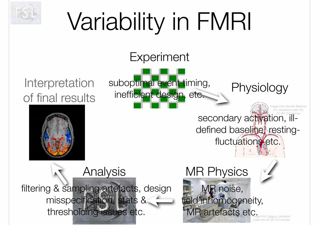
FMRI inferential pathExperiment

MR PhysicsAnalysis

PhysiologyInterpretation of final results

Image from mos.ru, released under the CC BY 4.0 license

Image from Servier Medical Art, released under the

CC BY 3.0 license

Interpretation of final results

Variability in FMRIExperiment

MR PhysicsAnalysis

Physiology

MR noise, field inhomogeneity, MR artefacts etc.

filtering & sampling artefacts, design misspecification, stats & thresholding issues etc.

suboptimal event timing, inefficient design, etc.

secondary activation, ill-defined baseline, resting-

fluctuations etc.

Image from Servier Medical Art, released under the

CC BY 3.0 license

Image from mos.ru, released under the CC BY 4.0 license

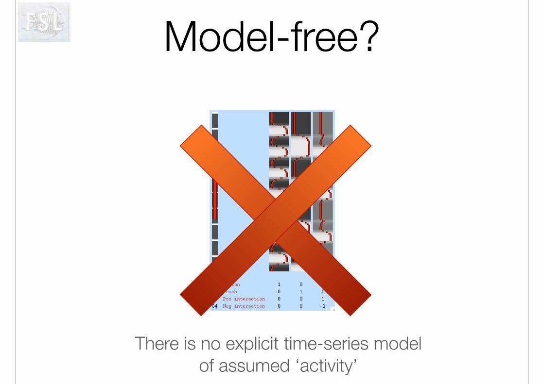
There is no explicit time-series model of assumed ‘activity’

Model-free?

Model-free?

Yi = SiA i + Ei , where Ei·j ⇠ N(0,σ

2Y I)

There is an underlying mathematical (generative) model

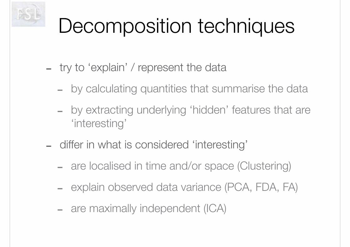
Decomposition techniques

- try to ‘explain’ / represent the data

- by calculating quantities that summarise the data

- by extracting underlying ‘hidden’ features that are ‘interesting’

- differ in what is considered ‘interesting’

- are localised in time and/or space (Clustering)

- explain observed data variance (PCA, FDA, FA)

- are maximally independent (ICA)

Melodic

multivariate linear decomposition:

Melodic


time

FMRI data

space

x

spacecom

ponents

spatial maps

=

components

time

courses

time

Melodic


time

FMRI data

space

x

spacecom

ponents

spatial maps

=

components

time

courses

time

Melodic


Data is represented as a 2D matrix and decomposed into components

time

FMRI data

space

x

spacecom

ponents

spatial maps

=

components

time

courses

time

Melodic


Data is represented as a 2D matrix and decomposed into components

time

FMRI data

space

Y = βX x

What are components?

- express observed data as linear combination of spatio-temporal processes

- techniques differ in the way data is represented by components

≈

×

+

×

+

×

Spatial ICA for FMRI

- data is decomposed into a set of spatially

independent maps and a set of time-courses

McKeown et al. HBM 1998

x

space

components

spatial maps

time

space

FMRI data=

components

time

courses

time

Independence

PCA vs. ICA ?Simulated

Data

(2 components, slightly different timecourses)

PCA

• Timecourses orthogonal

• Spatial maps and timecourses “wrong”


Data


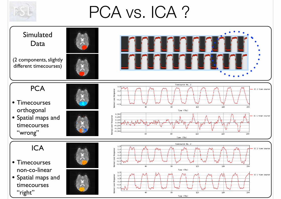
ICA

• Timecourses non-co-linear

• Spatial maps and timecourses “right”

PCA

• Timecourses orthogonal

• Spatial maps and timecourses “wrong”


Data


PCA vs. ICA

• PCA finds projections of maximum amount of variance in Gaussian data (uses 2nd order statistics only)

• Independent Component Analysis (ICA) finds projections of maximal independence in non-Gaussian data (using higher-order statistics)

−5 −4 −3 −2 −1 0 1 2 3 4 5−5

−4

−3

−2

−1

0

1

2

3

4

5

Gaussian data

non-Gaussian data

PCA vs. ICA

• PCA finds projections of maximum amount of variance in Gaussian data (uses 2nd order statistics only)

• Independent Component Analysis (ICA) finds projections of maximal independence in non-Gaussian data (using higher-order statistics)

−5 −4 −3 −2 −1 0 1 2 3 4 5−5

−4

−3

−2

−1

0

1

2

3

4

5

−5 −4 −3 −2 −1 0 1 2 3 4 5−5

−4

−3

−2

−1

0

1

2

3

4

5

−1.0 −0.5 0.0 0.5 1.0

−1.0

−0.5

0.0

0.5

1.0

x = cos(z)

y=

sin(

z)

Plot x vs. y

. .....

.

.

.

....

. ... .

.

. .. ...

..

.....

.

..

...

..

.

. ...

....

....... .

..

...

.... ...

...

. .....

...

....

.

... ...

..

...... .

..

.... .

..... .

.....

..

..

.

.. ... ... .... .

.

.

.....

.....

..

... ...... ..

. ..

..... .. .

.. ...

.

.

....... .. .. .

... ..

..... .. ...

.. .. ...

... ... ... . ..

...

.. .. ... . ....

...

..

. ..

.. .

..

.

. .. .

..

...

... ...

.

....

..

.....

... .. ..

.

. ...... .....

.... ... .....

. .. .

..

...

.. ..... ..... ..

.

.. ...

... ...

...

. ... .... ...

..

...... .

....

.

.. ... .... ... .

....

.

.. ..

..

....... . .

. . . ..

.....

..

...

.

. ...

..

.

... .

.

...

.

...

.. .

... .. .

.

.... ....

.

.. ...

....

. .... ..

...

..

.

..

.. ...

.

..

...

..

r=0.000

Correlation vs. independence

• de-correlated signals can still be dependent

( )

0.0 0.5 1.0 1.5

0.0

0.5

1.0

1.5

x2 = cos(z)2

y2=

sin(

z)2

high order correlations

. .... . ..

. . .. .. ... ...

.. ...

.....

...

..

...

.

.

.

. ...

..

..

.

....

...

.

..

..

.

..

.

...

..

.

...

.. .

.

.

.

..

..

.

..

..

..

.

.

..

...

..

.

.

.

..

. .

.

.

.

...

.

.

...

.

.

.

.

.

..

.

.... .

.

.....

.

...

.

.

. .

...

.

.

..

..

...

...

.

..

.

..

.. .

...

..

..

.

.

.

..

. .. . ..

.. ..

.. .

.

..

..

.

.... .

.

... .. .

.

..

..

... . ..

.... .

..... . ... . . .. ... . .. .. .. .. ... .. .. ... . . .. .

..

..

...

... . ..

. . .....

.

...

.

.

..

. ...

.

. ..

..

...

.

. .

.

..

..

.

.

.

..

.......

..

....

.

.

.

...

.

. .

....

.

..

..... ..

...

.

.

.

.

.

.

.

.

.

.

.

..

.

.

.....

.

.

...

...

.

...

.

.

. ..

.

.

.

...

.... .

..

..

.

.

..

..

.

.

. .

.

.

..

.

.

.

.

.

.

..

.

.

...

.

. .

.

.

. .

.. . .. .

.

.. .. .

. ..

.

.. ..

.

....

. . ... ..

...

..

... .. ... .. .. .. ..

r= −0.118

• higher-order statistics (beyond mean and variance) can reveal these dependencies

• Stone et al. 2002

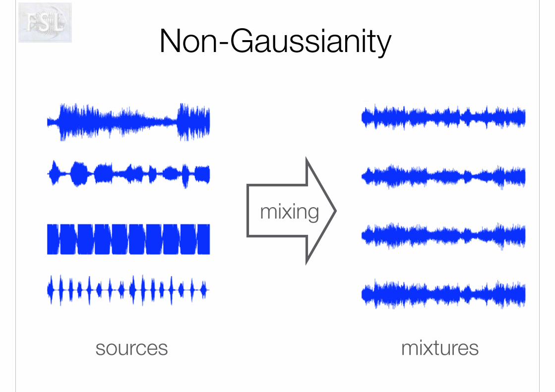
Non-Gaussianity

sources mixtures

mixing

mixing

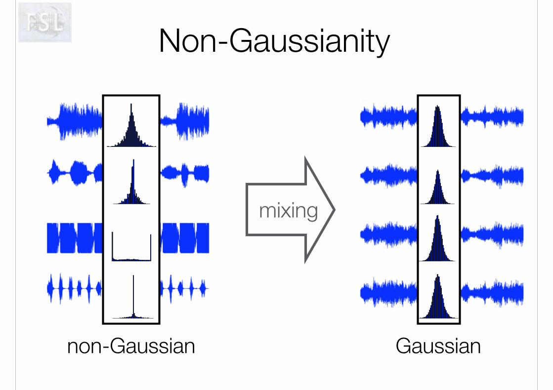
Non-Gaussianity

Gaussiannon-Gaussian

• Random mixing results in more Gaussian-shaped PDFs (Central Limit Theorem)

• conversely:

if mixing matrix produces less Gaussian-shaped PDFs this is unlikely to be a random result

➡ measure non-Gaussianity

• can use neg-entropy as a measure of non-Gaussianity

Hyvärinen & Oja 1997

ICA estimation

ICA estimation

- need to find an unmixing matrix such that the dependency between estimated sources is minimised

- need (i) a contrast (objective/cost) function to drive the unmixing which measures statistical independence and (ii) an optimisation technique:

- kurtosis or cumulants & gradient descent (Jade)

- maximum entropy & gradient descent (Infomax)

- neg-entropy & fixed point iteration (FastICA)

Overfitting & thresholding

The ‘overfitting’ problem

fitting a noise-free model to noisy observations:

- no control over signal vs. noise (non-interpretable results)

- statistical significance testing not possible

GLM analysis standard ICA (unconstrained)

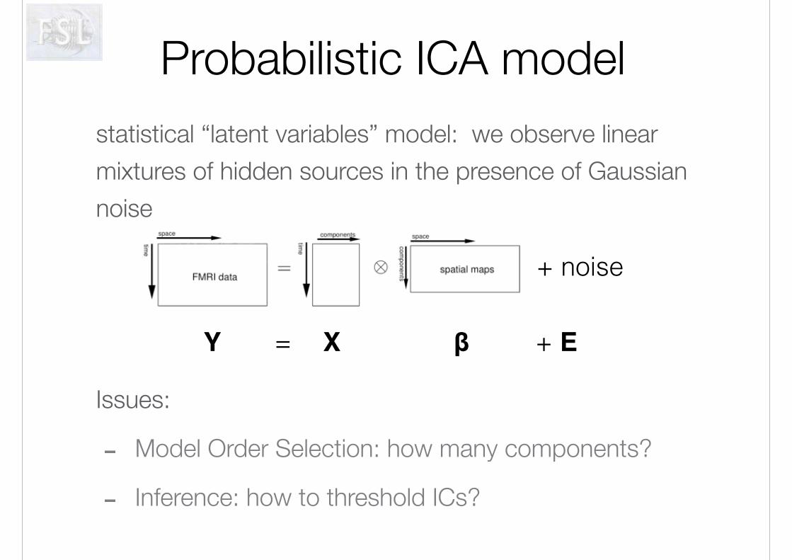
statistical “latent variables” model: we observe linear

mixtures of hidden sources in the presence of Gaussian

noise

Probabilistic ICA model

Issues:

- Model Order Selection: how many components?

- Inference: how to threshold ICs?

Y = βX

+ noise

+ E

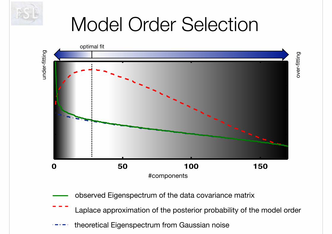
Model Order Selection

under-fitting: the amount of explained data variance is insufficient to obtain good estimates of the signals

15

optimal fitting: the amount of explained data variance is sufficient to obtain good estimates of the signals while preventing further splits into spurious components

33

over-fitting: the inclusion of too many components leads to fragmentation of signal across multiple component maps, reducing the ability to identify the signals of interest

165

‘How many components’?

Model Order Selection

#components

over

-fitt

ing

und

er-fi

ttin

g

observed Eigenspectrum of the data covariance matrix

theoretical Eigenspectrum from Gaussian noise

Laplace approximation of the posterior probability of the model order

optimal fit

0 50 100 1500.2

0.4

0.6

0.8

Thresholding

Thresholding

- classical null-hypothesis testing is invalid

- data is assumed to be a linear combination of signals and noise

- the distribution of the estimated spatial maps is a mixture distribution!

−2 −1 0 1 2 3 4 5 6 7

1 2 3 4 5 6

right tail

−2.5−2−1.5−1

left tail

Alternative Hypothesis Test

- use Gaussian/Gamma mixture model fitted to the histogram of intensity values (using EM)

What about overlap?

What about overlap?

⇢ = 0.5

Sources

⇢ < 0.1

Sources + noise

ICA solution

⇢ = 0

after thresholding

⇢ ⇡ 0.5

resting state fmri and ica

Documents