gssi-radan 7 manual - gssi inc. | georadar in consideration of the payment of a license fee, you are...
TRANSCRIPT


Geophysical Survey Systems, Inc. RADAN® 7 Manual
MN43-199 Rev G
Limited Warranty, Limitations of Liability and Restrictions Geophysical Survey Systems, Inc. hereinafter referred to as GSSI, warrants that for a period of 24 months from the delivery date to the original purchaser this product will be free from defects in materials and workmanship. EXCEPT FOR THE FOREGOING LIMITED WARRANTY, GSSI DISCLAIMS ALL WARRANTIES, EXPRESS OR IMPLIED, INCLUDING ANY WARRANTY OF MERCHANTABILITY OR FITNESS FOR A PARTICULAR PURPOSE. GSSI's obligation is limited to repairing or replacing parts or equipment which are returned to GSSI, transportation and insurance pre-paid, without alteration or further damage, and which in GSSI's judgment, were defective or became defective during normal use. GSSI ASSUMES NO LIABILITY FOR ANY DIRECT, INDIRECT, SPECIAL, INCIDENTAL OR CONSEQUENTIAL DAMAGES OR INJURIES CAUSED BY PROPER OR IMPROPER OPERATION OF ITS EQUIPMENT, WHETHER OR NOT DEFECTIVE. Before returning any equipment to GSSI, a Return Material Authorization (RMA) number must be obtained. Please call the GSSI Customer Service Manager who will assign an RMA number. Be sure to have the serial number of the unit available. Copyright © 2011-2017 Geophysical Survey Systems, Inc. All rights reserved including the right of reproduction in whole or in part in any form Published by Geophysical Survey Systems, Inc. 40 Simon Street Nashua, New Hampshire 03060-3075 USA Printed in the United States SIR, RADAN and UtilityScan are registered trademarks of Geophysical Survey Systems, Inc.

Geophysical Survey Systems, Inc. RADAN® 7 Manual
MN43-199 Rev G
Limited Use License Agreement You should carefully read the following terms and conditions before opening this package. By opening this package you are agreeing to become bound by the terms of this agreement and indicating your acceptance of these terms and conditions. If you do not agree with them, you should return the package unopened to Geophysical Survey Systems, Inc. Geophysical Survey Systems, Inc. (GSSI), an OYO Corporation, provides the computer software ("RADAN 7") contained on the medium in this package, and licenses its use. You assume full responsibility for the selection of RADAN 7 to achieve your intended results and for the installation, use and results obtained from the Program. License a) In consideration of the payment of a license fee, you are granted a personal, non-transferable license to use RADAN 7 under the terms stated in this Agreement. You own the USB or other physical media on which RADAN 7 is provided under this Agreement, but all title and ownership of RADAN 7 and enclosed related documentation "("Documentation"), and all other rights not expressly granted to you under this Agreement, remain in Geophysical Survey Systems, Inc.; b) RADAN 7 is a single-user license; c) You and your employees and agents are required to protect the confidentiality of RADAN 7. You may not distribute or otherwise make RADAN 7 or Documentation available to any third party; d) You may not copy or reproduce RADAN 7 or Documentation for any purpose except you may make one (1) copy of RADAN 7 if RADAN 7 is not copy-protected, in machine readable or printed form for backup purposes only in support of your use of RADAN 7. You must reproduce and include the Geophysical Survey Systems, Inc. copyright notice on the Backup copy of RADAN 7; e) Any portion of RADAN 7 merged into or used in conjunction with another program will continue to be the property of GSSI and subject to the terms and conditions of this Agreement. You must reproduce and include the copyright notice on any portion merged into or used in conjunction with another program; f) You may not sublease, assign, or otherwise transfer RADAN 7 or this license to any other person without the prior written consent of GSSI. Any authorized transferee of RADAN 7 will be bound by the terms and conditions of this Agreement; and g) You acknowledge that you are receiving only a Limited License to use RADAN 7 and Documentation and GSSI retains title to RADAN 7 and Documentation. You acknowledge that GSSI has a valuable proprietary interest in RADAN 7 and Documentation. You may not use, copy, modify, or transfer RADAN 7 or Documentation, or any copy, modification, or merged portion, in whole or in part, except as expressly provided for this Agreement. If you transfer possession of any copy, modification, or merged portion of RADAN 7 or Documentation to another party, your license is automatically terminated.
Term The license granted to you is effective until terminated. You may terminate it at any time by returning RADAN 7 and Documentation to GSSI together with all copies, modifications, and merged portions in any form. The license will also terminate upon conditions set forth elsewhere in this Agreement or if you fail to comply with any term or condition of this Agreement. You agree upon such termination to return RADAN 7 and Documentation to GSSI together with all copies, modifications, and merged portions in any form. Upon termination, GSSI can also enforce any rights provided by law. The provisions of this Agreement which protect the proprietary rights of GSSI will continue in force after termination.

Geophysical Survey Systems, Inc. RADAN® 7 Manual
MN43-199 Rev G
Limited Warranty GSSI warrants as the sole warranty provided to you that the USB on which RADAN 7 is furnished will be free from defects in materials and workmanship under normal use and conditions for a period of ninety (90) days from the date of delivery to you as evidenced by a copy of your receipt. No distributor, dealer, or any other entity or person is authorized to expand or alter either this warranty or this Agreement; any such representation will not bind GSSI. GSSI does not warrant that the functions contained in RADAN 7 will meet your requirements or that the operation of RADAN 7 will be uninterrupted or error-free. Except as stated above in this section, RADAN 7 and Documentation are provided "as is" without warranty of any kind, either express or implied, including but not limited to, the implied warranties of merchantability and fitness for a particular purpose. You assume the entire risk as to the quality and performance of the program and documentation. Should the program prove defective, you (and not GSSI or any authorized GSSI distributor or dealer) assume the entire cost of all necessary servicing, repair, or correction. This warranty gives you specific legal rights, and you may also have other rights which vary from state to state. Some states do not allow the exclusion of implied warranties, so the above exclusion may not apply to you.
Limitation Of Remedies GSSI's entire liability and your exclusive remedy will be: a) The replacement of any USB not meeting GSSI's "Limited Warranty" explained above and which is returned to GSSI with a copy of your receipt; or b) If GSSI is unable to deliver a replacement USB which conforms to the warranty provided under this Agreement, you may terminate this Agreement by returning RADAN 7 and Documentation to GSSI and your license fee will be refunded. IMPORTANT: If you must ship RADAN 7 and Documentation to GSSI, you must prepay shipping and either insure RADAN 7 and Documentation or assume all risk of loss or damage in transit. To replace a defective USB during the ninety (90) day warranty period, if you are returning the medium to GSSI, please send us your name and address, the defective medium and a copy of your receipt at the address provided below. In no event will GSSI be liable to you for any damages, direct, indirect, incidental, or consequential, including damages for any lost profits, lost savings, or other incidental or consequential damages, arising out of the use or inability to use RADAN 7 and Documentation, even if GSSI has been advised of the possibility of such damages, or for any claim by any other party. Some states do not allow the limitation or exclusion of liability for incidental or consequential damages, so the above limitation or exclusion many not apply to you. In no event will GSSI's liability for damages to you or any other person ever exceed the amount of the license fee paid by you to use RADAN 7, regardless of the form of the claim.
U.S. Government Restricted Rights RADAN 7 and Documentation are provided with restricted rights. Use, duplications, or disclosure by the U.S. Government is subject to restrictions as set forth in subdivision (b)(3)(ii) of the Rights in Technical Data and Computer Software clause at 252.277-7013. Contract/manufacturer is Geophysical Survey Systems, Inc., 40 Simon Street, Nashua, New Hampshire 03060-3075.
GENERAL This Agreement is governed by the laws of the State of New Hampshire (except federal law governs copyrights and registered trademarks). If any provision of this Agreement is deemed invalid by any court having jurisdiction, that particular provision will be deemed deleted and will not affect the validity of any other provision of this Agreement. Should you have any questions concerning this Agreement, you may contact GSSI by writing Geophysical Survey Systems, 40 Simon Street, Nashua, New Hampshire 03060-3075 U.S.A.` You acknowledge that you have read this agreement, understand it and agree to be bound by its terms and conditions. You further agree that it is the complete and exclusive statement of the Agreement between you and GSSI which supersedes any proposal or prior Agreement, oral or written, and any other communications between us relating to the subject matter of this Agreement.

Geophysical Survey Systems, Inc. RADAN® 7 Manual
MN43-199 Rev G
Table of Contents
How to Use This Manual: Must Read ........................................................................................1
System Requirements and Notes ..............................................................................................2 Recommended System Requirements for RADAN 7 ................................................. 2 Minimum System Requirements for RADAN 7 ............................................................. 2 What Data Can Be Processed with RADAN 7 ................................................................ 2 RADAN 7 is Not Currently Recommended for Users of ............................................. 2
Section 1: Getting Started ............................................................................................................3 GSSI Activation Policies ...................................................................................................................... 3 General Description ............................................................................................................................. 3 Installing RADAN 7 ............................................................................................................................... 4
Installation Instructions ........................................................................................................ 4 Launching/Activating/Validating the RADAN 7 Software ...................................................... 6
Launching the Software for the First Time .................................................................... 6 Activating the Software ........................................................................................................ 7 Software Demo ........................................................................................................................ 7 Validating the Software ........................................................................................................ 7 Updating the Software ......................................................................................................... 8
Section 2: Using RADAN 7 ............................................................................................................9 Recommended Modules .................................................................................................................... 9 Setting up a Laptop/PC and Data Transfer .................................................................................. 9 Example Data ...................................................................................................................................... 10 Launching RADAN 7, the Main Screen, and Configuring RADAN ..................................... 10
Launching the Software ..................................................................................................... 10 The Main Screen .................................................................................................................... 11 Configuring the Software: Setting Global Parameters ............................................ 12
Section 3: Navigating Through RADAN 7 – The Menus, Panes and Ribbons ....... 15 Menus ...................................................................................................................... 15 GSSI Button .......................................................................................................................................... 15 Panes and Tables .................................................................................................... 28 My Files, Processes & Proc. List Pane ........................................................................................... 28 Properties Pane .................................................................................................................................. 30 Table Pane ........................................................................................................................................... 37

Geophysical Survey Systems, Inc. RADAN® 7 Manual
MN43-199 Rev G
Ribbons: Structure and Functions ......................................................................... 39 Home Ribbon ...................................................................................................................................... 39 View Ribbon ........................................................................................................................................ 42 Easy Processing Ribbon ................................................................................................................... 43 Processing Ribbon ............................................................................................................................ 50 2D Interactive...................................................................................................................................... 77 StructureScan Ribbon ...................................................................................................................... 83 RoadScan Ribbon .............................................................................................................................. 86 BridgeScan Ribbon ........................................................................................................................... 95 Horn BridgeScan Ribbon............................................................................................................... 105 Dual Polarity Horn BridgeScan Ribbon .................................................................................... 116 Google Earth® Ribbon .................................................................................................................... 127
Section 4: Application-Specific Displays ...........................................................................131 Reader ................................................................................................................................................. 131 Standard Processing ....................................................................................................................... 134 RADAN 7 for StructureScan Mini ................................................................................................ 135
GSSI Button .......................................................................................................................... 135 RADANMini Home Ribbon ............................................................................................. 136 3D Volume Options Ribbon ........................................................................................... 140
UtilityScan DF ................................................................................................................................... 141 GSSI Button .......................................................................................................................... 141 UtilityScan DF Applications Ribbon ............................................................................ 142 Google Earth® Ribbon ...................................................................................................... 147 3D Volume Options Ribbon ........................................................................................... 148
RoadScan ............................................................................................................................................ 150 GSSI Button .......................................................................................................................... 150 Home Ribbon ...................................................................................................................... 151 View Ribbon ......................................................................................................................... 154 Processing ............................................................................................................................ 155 2D Interactive ...................................................................................................................... 157 Google Earth® Ribbon ...................................................................................................... 162
Ground-Coupled BridgeScan ...................................................................................................... 164 GSSI Button .......................................................................................................................... 164 Home Ribbon ...................................................................................................................... 165 View Ribbon ......................................................................................................................... 168 Processing ............................................................................................................................ 169 2D Interactive ...................................................................................................................... 172 Google Earth® Ribbon ...................................................................................................... 177
Horn BridgeScan .............................................................................................................................. 180 GSSI Button .......................................................................................................................... 180 Home Ribbon ...................................................................................................................... 181 View Ribbon ......................................................................................................................... 184 Processing ............................................................................................................................ 185 2D Interactive ...................................................................................................................... 188 Google Earth® Ribbon ...................................................................................................... 193

Geophysical Survey Systems, Inc. RADAN® 7 Manual
MN43-199 Rev G
Dual Polarization Horn BridgeScan ........................................................................................... 196 GSSI Button .......................................................................................................................... 197 Home Ribbon ...................................................................................................................... 197 View Ribbon ......................................................................................................................... 200 Processing ............................................................................................................................ 201 2D Interactive ...................................................................................................................... 205 Google Earth® Ribbon ...................................................................................................... 210
Section 5: Basic Processing Tutorials ..................................................................................213 Using the Proc. Lists Tab ............................................................................................................... 213 Creating a Manual Grid .................................................................................................................. 214 Creating a Super Grid ..................................................................................................................... 216 Appending Files ............................................................................................................................... 218 Basic 3D Grid Navigation .............................................................................................................. 219 Interactive Processing .................................................................................................................... 223 Time Zero Correction ..................................................................................................................... 226 FIR Filtering ........................................................................................................................................ 227 Migration ............................................................................................................................................ 229 CMP Velocity Analysis and Migration ....................................................................................... 232 Distance Normalization ................................................................................................................. 234 Deconvolution .................................................................................................................................. 235 Horizontal Scaling ........................................................................................................................... 237 Surface Normalization ................................................................................................................... 238 Range Gain ......................................................................................................................................... 239
Section 6: Processing Specific Applications .....................................................................241 StructureScan ................................................................................................................................... 241
Processing the Data .......................................................................................................... 241 View Depth Slices .............................................................................................................. 242 3-D View ................................................................................................................................ 243
RoadScan ............................................................................................................................................ 244 Creating the Calibration File .......................................................................................... 244 Processing the Road File ................................................................................................. 245 Layer/Target Picking ......................................................................................................... 246
BridgeScan ......................................................................................................................................... 247 Preparing the Data ............................................................................................................ 247 Editing Target Picks ........................................................................................................... 249
Appendix A: Sample Data .......................................................................................................251
Appendix B: GSSI Naming Convention ..............................................................................255
Appendix C: Dielectric Constants ........................................................................................257
Appendix D: Glossary of Terms .............................................................................................259
List of References and Suggestions for Further Reading ............................................265

Geophysical Survey Systems, Inc. RADAN® 7 Manual
MN43-199 Rev G

Geophysical Survey Systems, Inc. RADAN® 7 Manual
MN43-199 Rev G 1
How to Use This Manual: Must Read This manual is designed for both experienced and novice users of RADAN® 7. This manual is broken up into five sections to help you find answers you are looking for. Some processes may be duplicated in different sections. This is designed to assist you with quickly finding the help you might need based upon the question(s) you may be asking. Section 1: Getting Started is General Description of the software, general requirements, getting started, installing and activating the software Section 2: Using RADAN 7 is basic use of RADAN 7, launching the software, updating the software, and navigating through the screens Section 3: Navigating Through RADAN 7 is a description of every screen and menu option in RADAN 7. Section 4: Application-Specific Display is a description of the display options available for specific applications. Section 5: Basic Processing/Tutorials is basic processing steps/tutorials for any set of data. Section 6: Processing Specific Applications is basic processing for StructureScan, RoadScan, and BridgeScan applications.

Geophysical Survey Systems, Inc. RADAN® 7 Manual
MN43-199 Rev G 2
System Requirements and Notes
Recommended System Requirements for RADAN 7 • Microsoft Windows® 7 (32 or 64 bit) • Intel Core i5 (or better) processor • 3+ GB system memory • 500+ GB hard drive with a minimum of 100 GB available space • 256+ MB dedicated graphics chipset with OpenGL drivers (Note: We only support NVidia and
Intel graphics chipsets)
Minimum System Requirements for RADAN 7 • Version 7.0.4.9 is the last version compatible with Microsoft Windows® XP. All later versions
require Microsoft Windows® Vista or higher. • 1.0+ GHz Pentium 4 (Note: We do not support single core single thread processors) • 2 GB system memory • 160 GB hard drive with a minimum of 20 GB available space • 128 MB graphics chipset with OpenGL drivers (Note: We only support NVidia and Intel graphics
chipsets.)
What Data Can Be Processed with RADAN 7 • RADAN 7 is necessary for viewing of SIR 4000, SIR® 30, SIR® 40, and UtilityScan-DF data. It
adds capabilities to view and process the new raw data format of these newer SIR systems. • SIR 4000 (2D dzt, 3D b3d, GPS dzg) • SIR 3000 (2D dzt, 3D b3d, GPS tmf, plt and gga text from the SDR data logger) • UtilityScan DF (2D dzt, GPS dzg) • SIR 20 (2D dzt, 3D b3d, GPS tmf and gga text from the SDR data logger) • StructureScan Optical data • Individual profiles of older systems such as SIR 10 and SIR 2000 • Files processed by RADAN 4.x RADAN 5.x and RADAN 6.x • 3D files which have the Microsoft Access (mdb) based database
RADAN 7 is Not Currently Recommended for Users of • StructureScan users working with the black pad • Terravision:
o Y Gain Equalization is not currently implemented in RADAN 7 o RADAN 7 will not properly import GPS for Terravision but will read Terrravision files that
have been opened in RADAN 6. • SIR 20 control units. This should not be confused with SIR 20 post processing systems.
RADAN 7 is designed to work with SIR 20 data, but not on the Toughbooks running the SIR 20 operating software. RADAN 6 remains the control interface for the SIR 20 systems.
• It does not contain a replacement for controlling SIR 20 systems. All hardware control features of RADAN 6.6 and earlier have been removed from RADAN 7.
• CF-29 and earlier Toughbook® do not meet the minimum specifications for RADAN 7.
Geophysical Survey Systems, Inc. RADAN® 7 Manual
MN43-199 Rev G 3
Section 1: Getting Started Thank you for purchasing RADAN® 7. The packing list included with the shipment lists all of the items in your order. The RADAN 7 program and example files are stored on a single USB drive.
GSSI Activation Policies The RADAN 7 license includes one license for installation on one computer.
General Description RADAN 7 software was designed to process, view, and document data collected with products from GSSI. RADAN 7 module can perform the following functions:
• Display multiple screens of radar data as line scan, wiggle trace, and/or oscilloscope. • Manipulate color table and color transform parameters to enhance data display. • Edit file headers and distance markers. • Process individual files or multiple files. • Modify or restore data gains. • Correct position (shift data scans along the time axis). • Provide horizontal scaling and distance normalization. • Incorporate topographic changes with top surface normalization. • Display the frequency spectrum of data. • Apply Infinite Impulse Response (IIR) and Finite Impulse Response (FIR) filters. • Perform migration. • Perform predictive deconvolution. • Perform envelope processing functions (Hilbert Transform). • Velocity analysis. • Local peak interpretation. • Interactive interpretation. • Print to all Windows supported printers. • Export data as image, .dxf, .shp, .kml, or .csv files.

Geophysical Survey Systems, Inc. RADAN® 7 Manual
MN43-199 Rev G 4
Installing RADAN 7 It is highly recommended to be connected to the internet when installing the software so that activation can take place at the time of installation. If there is not a connection, contact GSSI for other activation instructions.
1 Insert the RADAN 7 Installation USB into one of your computer’s USB ports.
2 The installation program should start automatically. If the program did start automatically, skip to Step 5. If it did not start automatically skip to Step 3.
3 Using Windows Explorer, double-click the external drive that contains the RADAN 7 Installation USB.
4 Find the Start Icon and double-click it.
5 Follow on-screen instructions:
a) Install RADAN 7: Select this option to install the software onto the computer.
b) Technical Support Web Site Info: This will open a PDF file that has excellent information about how to use our support web site. It is highly recommended that the user opens, saves, and prints this file.
c) GSSI Contacts: This will open a PDF file of essential contacts at GSSI. It is highly recommended that the user opens, saves, and prints this file.
Installation Instructions After you have selected Install RADAN 7 from the Main menu, you will see the following screens. Click Install > Accept > Next > OK or Finish through all the screens.

Geophysical Survey Systems, Inc. RADAN® 7 Manual
MN43-199 Rev G 5
3
1 2
5
Note: Depending upon the age of your computer, your operating system (Windows XP, Windows Vista, Windows 7, or Windows 8), and the age of your operating system, you may get other screens asking you to install other software. You should accept these, or if you have questions, contact your IT person or GSSI.
4

Geophysical Survey Systems, Inc. RADAN® 7 Manual
MN43-199 Rev G 6
Launching/Activating/Validating the RADAN 7 Software
Launching the Software for the First Time When launching the software for the first time, it will ask which language to use.
1 Highlight the language.
2 Select either: • Show this form again: English will be the default language,
and a prompt will appear the next time the software is launched.
• Use the selected language: The language that is highlighted will be used on subsequent launches of the software.
• Use the default language: English is the default language and will be used on subsequent launches of the software.
The language may be changed at any time by:
1 Clicking the GSSI Button.
2 Clicking on Options.

Geophysical Survey Systems, Inc. RADAN® 7 Manual
MN43-199 Rev G 7
Activating the Software After installing the software, RADAN 7 will automatically start. The first time the software is run, the user will be asked to activate it. The computer MUST be connected to the internet to activate the software.
1 From the label located on the back of the USB case, input the Product Key and the Serial Number into the appropriate fields.
2 The Computer Name is pre-filled by GSSI (this is the name of the user’s computer from their computer system).
3 Enter a valid email address.
4 Click Activate/Validate your Product Key.
Software Demo If the software is not activated after installation it will run as a demo for 30 days or 32 activations (whichever comes first). If the software is not activated before the demo expires, the user will have access to a Reader version of the software with options to view data in 2D or 3D depth slices, change colors, and save the data as jpg image files.
Validating the Software At times, upon launching RADAN 7, the software will ask to test the license. Click Yes and a pre-populated screen will appear. Simply click Continue with RADAN 7. An internet connection is needed to test the license.
Note: If the software is not activated at this time, the adjacent screen will appear at the launching of the software until it is activated. After activating the software, an internet connection is not needed to run the software.
Geophysical Survey Systems, Inc. RADAN® 7 Manual
MN43-199 Rev G 8
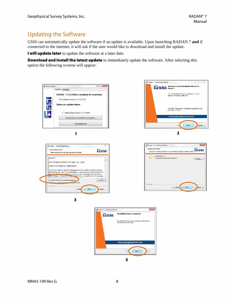
Updating the Software GSSI can automatically update the software if an update is available. Upon launching RADAN 7 and if connected to the internet, it will ask if the user would like to download and install the update. I will update later to update the software at a later date. Download and Install the latest update to immediately update the software. After selecting this option the following screens will appear:
1 2
3
5

Geophysical Survey Systems, Inc. RADAN® 7 Manual
MN43-199 Rev G 9
Section 2: Using RADAN 7
Recommended Modules RADAN 7 is purchased in modules. RADAN 7 MAIN includes Easy Processing, Processing, and Google Earth. Below is a table showing recommended features for some common applications.
Applications
Modules
Utility Scanning
Utility Locating
w/UtilityScan DF
Structure
Scanning
Structure Scanning w/SSMini
Road Scanning
Bridge Scanning
BridgeScan w/Air Launched (BAL) Antenna
3D (3D) X X X X
StructureScan (SID) X
RADAN 7 for StructureScan Mini
X
UtilityScan DF X
RoadScan (RSA) X
BridgeScan (BQA) X
Horn BridgeScan (BAL) X
Dual Pol. Horn BridgeScan (BAL) X
Modules are broken down by application. You can choose to purchase RADAN 7 MAIN with the application modules or they may be purchased separately. Each application module includes specialized processing and viewing options. For more information about each module see Section 6: Processing Specific Applications.
Setting up a Laptop/PC and Data Transfer Suggestions for data organization:
• Create a different folder for each project. The project folder will contain raw, unprocessed data that was collected and saved.
• Create a Processed or Output folder within each of the project folders. This folder will contain files that were processed from the raw, unprocessed data.
• After creating the folders, copy raw files from the device to the appropriate project folder. Folders may be organized by the user’s own set of rules. However, it is necessary to know the folder names and locations when configuring RADAN 7 at the start of each project.
Note: A separate manual is available for the RADAN 7 for StructureScan Mini and RADAN 7 for UtilityScan DF Module.

Geophysical Survey Systems, Inc. RADAN® 7 Manual
MN43-199 Rev G 10
Example Data Example data for use with RADAN 7 is available for download from the GSSI Technical Support website. Refer to the Basic Processing/Tutorials sections for more information about the examples data.
Launching RADAN 7, the Main Screen, and Configuring RADAN
Launching the Software Launch RADAN 7 by double-clicking the RADAN 7 icon. The following screen is displayed:
1 GSSI Button
2 My Files/Processes/Proc. List Pane
3 Ribbons
4 Data Pane
5 Global Settings/Properties Pane
6 Tables Pane
3 2 4 1 5 6

Geophysical Survey Systems, Inc. RADAN® 7 Manual
MN43-199 Rev G 11
The Main Screen Most of the options below will be detailed throughout Section 3: Navigating Through RADAN 7.
GSSI Button Clicking on the GSSI Button allows the user to:
• Open a File/Project • Assemble Files • Import GPS • Save a File/Project • Save As a File/Project under a different name
or format • Export data • Print data • Close a File/Project • Close All Open Files • Open a previously processed File/Project • Options to change languages • Exit RADAN 7 Software
My Files, Processes & Proc. List Pane There are three tabs in this section: My Files Tab: This tab will provide quick access to project data, recently processed data and GSSI example data. Click on the box to the left of the filename to open the file. An opened file can be also be closed by unchecking the box to the left of the filename. Processes Tab: This tab contains all of the available processes organized in a tree structure. Expand the tree and click on a process to access a process. Proc. Lists Tab: The options located in this area provide a quicker way to apply more commonly used processes to the data. GSSI has created these commonly used processes as macros, which are a series of steps and/or options put together as one option. Custom process lists can also be made and are located in this area.
Ribbon This area contains all the major viewing and processing options available in RADAN 7. Tabs in the Ribbon are also broken down by application.
Data Pane This is where data are displayed when a file is opened. This screen can contain multiple files, each in its own tab.
Geophysical Survey Systems, Inc. RADAN® 7 Manual
MN43-199 Rev G 12
Global Settings/Properties Pane Global Settings: This area will display Global Parameters for all files in a particular project prior to opening any files and allow you to switch between available Application Displays. Properties Pane: File Header, Window Settings, and Data Channel Properties for a specific file will also appear here when selected from the Other Windows Group in the Home Ribbon.
Table Pane Depending upon the type of data that is being processed, this pane will display the database and allow editing of the information in a data file. More information about this is located in the Basic Processing/Tutorials section.
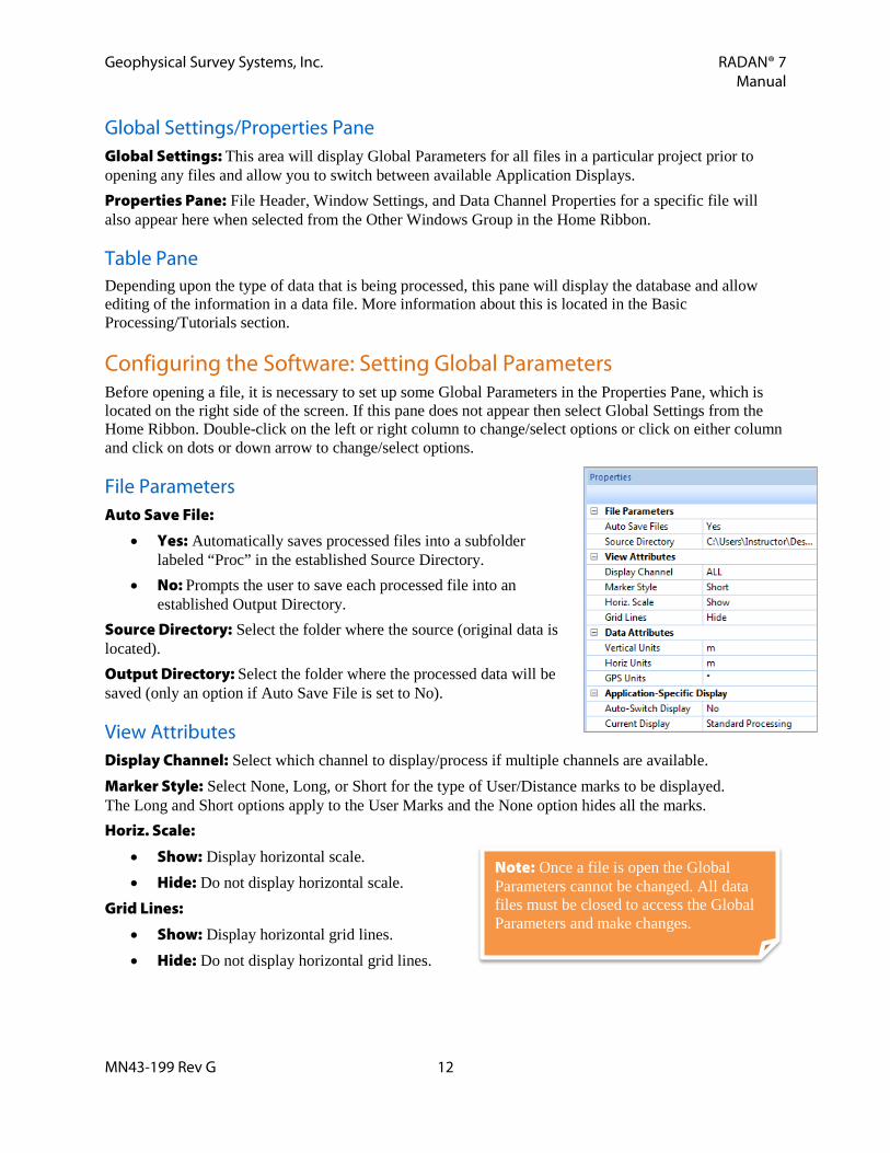
Configuring the Software: Setting Global Parameters Before opening a file, it is necessary to set up some Global Parameters in the Properties Pane, which is located on the right side of the screen. If this pane does not appear then select Global Settings from the Home Ribbon. Double-click on the left or right column to change/select options or click on either column and click on dots or down arrow to change/select options.
File Parameters Auto Save File:
• Yes: Automatically saves processed files into a subfolder labeled “Proc” in the established Source Directory.
• No: Prompts the user to save each processed file into an established Output Directory.
Source Directory: Select the folder where the source (original data is located). Output Directory: Select the folder where the processed data will be saved (only an option if Auto Save File is set to No).
View Attributes Display Channel: Select which channel to display/process if multiple channels are available. Marker Style: Select None, Long, or Short for the type of User/Distance marks to be displayed. The Long and Short options apply to the User Marks and the None option hides all the marks. Horiz. Scale:
• Show: Display horizontal scale. • Hide: Do not display horizontal scale.
Grid Lines:
• Show: Display horizontal grid lines. • Hide: Do not display horizontal grid lines.
Note: Once a file is open the Global Parameters cannot be changed. All data files must be closed to access the Global Parameters and make changes.

Geophysical Survey Systems, Inc. RADAN® 7 Manual
MN43-199 Rev G 13
Data Attributes When a file is opened, the scale will default to whatever units were saved with the file. Vertical Units: Units for the vertical scale. Horiz Units: Units for the horizontal scale. GPS Units: Units for GPS information displayed in the tables, status bar, and 3D window.
Application-Specific Display Switch between displays that include processing and viewing options based on the selected application. Available displays are based on which modules of RADAN were purchased. Auto-Switch Display:
• No: Data will open in the currently selected display. • Yes: The display will change based on the data file opened. For example, if data collected with
the StructureScan Mini is opened while in the Standard Processing Display, the display will automatically switch to the RADAN 7 for SSMini display.
Current Display:
• Reader: Opens the RADAN Reader display, which allows you to view already processed 2D data as profiles and 3D data as depth slices. The color table, color transform, and display gain can also be modified. If targets or picks were added in one of the other displays they can be displayed as well. Displayed data can be saved as .jpg images. This display is available with any purchase of RADAN 7 and will become the only way of viewing data once the demo version of the software expires without activation.
• Standard Processing: This is the most inclusive display with access to all of the application-specific tabs as well as all 2D and 3D (with purchase of Interactive 3D Module) viewing and processing options.
• RADAN for StructureScan Mini: This is display that is designed specifically for data collected with the StructureScan Mini and includes the ability to instantly process data, do some additional processing, add interpretations, and export to a jpg or excel to quickly generate a report.
• UtilityScan DF: This is display that is designed specifically for data collected with the UtilityScan DF and includes the ability to instantly process data, do some additional processing, add interpretations, and export to a jpg or excel to quickly generate a report.
• RoadScan: Provides viewing and processing options for data collected specifically for determining pavement layer thickness.
• Ground-Coupled BridgeScan: This display is designed to process data specifically collected to determine bridge deterioration using a ground-coupled antenna.
• Horn BridgeScan: This display is designed to process data specifically collected to determine bridge deterioration using an air-launched horn antenna.
• Dual Pol. Horn BridgeScan: This display is designed to process data specifically collected to determine bridge deterioration using two air-launched horn antennas mounted at right-angles to one-another.

Geophysical Survey Systems, Inc. RADAN® 7 Manual
MN43-199 Rev G 14

Geophysical Survey Systems, Inc. RADAN® 7 Manual
MN43-199 Rev G 15
Section 3: Navigating Through RADAN 7 – The Menus, Panes and Ribbons
Menus
GSSI Button
Open 1 Click the GSSI Button. Open any previously opened
file by selecting a file in the Recent Data Files section, or click Open to select a file from the Source or Output folder.
2 If Open is clicked, click on the down arrow in the Files of Type section to open one of the following file formats: • .dzt: RADAN file, a single profile or 3D file
(default). • .bzx: a formally created Batch file, a group of .dzt
files to be viewed and processed together. • .sgy: SEGY format Files. • .s3d: a formally created Super 3D Project file, which
contains information on how to create a Super 3D file from individual 3D files.
• .m3d, .b3d: a 3D project file, created either by the system or manually.
3 Once a file type is selected, click on the file to open and click Open, or double-click on the file to open.

Geophysical Survey Systems, Inc. RADAN® 7 Manual
MN43-199 Rev G 16
Assemble Data File
Append Files This option appends files to create longer profiles. Select Append Files and browse (if necessary) to the folder where the files to append are located.
1 Enter a name for the file being created.
2 Select No Merge to keep each profile separate, and Yes Merge to combine the files into one file.
3 Click Next to continue or Cancel to cancel the process.
4 There will be two windows: Available Files in Folder are files available to append; and Files to Append are the files that will be appended. Adding Files To Append Together
• Click Add All to add every file from the left window to the right window.
• Click on a file and click Add to add a single file to the right window.
• Add multiple files at once by clicking on one file, then while holding the Ctrl key, click on the other files to add. Then click Add.
• If the files to add are grouped together, click on the first file, hold down the Shift key, and click on the last file in that group. Then click Add.
Removing Files
• Click Remove All to remove every file from the right window to the left window.
• Click on a file and click Remove to remove a single file from the right window.
• Remove multiple files at once by clicking on one file, then while holding the Ctrl key, click on the other files to remove. Then click Remove.
• If the files to remove are grouped together, click on the first file, hold down the Shift key, and click on the last file in that group. Then click Remove.
5 Click Back to return to the previous screen.
6 Click Finish to complete the process.
7 Click Cancel to cancel the process.

Geophysical Survey Systems, Inc. RADAN® 7 Manual
MN43-199 Rev G 17
Combine Channels If data were collected using multi-channels, the files may be combined for viewing.
1 After Combine Channels is selected from Assemble Data Files, browse (if necessary) to the folder where the files to combine for viewing are located.
2 Click Next to continue or Cancel to cancel the process.
3 There will be two windows: Available Files in Folder are files available to combine channel; and Files to Combine are the files that will be added to the combine channel. Adding Files To Combine Channels
• Click Add All to add every file from the left window to the right window.
• Click on a file and click Add to add a single file to the right window.
• Add multiple files at once by clicking on one file, then while holding the Ctrl key, click on the other files to add. Then click Add.
• If the files to add are grouped together, click on the first file, hold down the Shift key, and click on the last file in that group. Then click Add.
Removing Files
• Click Remove All to remove every file from the right window to the left window.
• Click on a file and click Remove to remove a single file from the right window. • Remove multiple files at once by clicking on one file, then while holding the Ctrl key, click on
the other files to remove. Then click Remove. • If the files to remove files are grouped together, click on the first file, hold down the Shift key,
and click on the last file in that group. Then click Remove.
4 Click Back to return to the previous screen.
5 Click Finish to complete the process.
6 Click Cancel to cancel the process.

Geophysical Survey Systems, Inc. RADAN® 7 Manual
MN43-199 Rev G 18
Batch of Files To run the same process for multiple files, create a batch file that contains these files. The process is run once and then run repeated for every file in the batch file. The batch file created will be a .bzx file and contain only the names of the files to batch together. It will NOT be a data file (.dzt) of the files combined together.
1 After Batch of Files is selected from Assemble Data Files, browse (if necessary) to the folder where the files to batch are located.
2 Enter a name for the batch file being created.
3 Click Next to continue or Cancel to cancel the process.
4 There will be two panes: Available Files in Folder are files available to append; and Batch Files are the files that will be batched together. Adding Files to the Batch
• Click Add All to add every file from the left window to the right window.
• Click on a file and click Add to add a single file to the right window.
• Add multiple files at once by clicking on one file, then while holding the Ctrl key, click on the other files to add. Then click Add.
• If the files to add are grouped together, click on the first file, hold down the Shift key, and click on the last file in that group. Then click Add.
Removing Files
• Click Remove All to remove every file from the right window to the left window.
• Click on a file and click Remove to remove a single file from the right window.
• Remove multiple files at once by clicking on one file, then while holding the Ctrl key, click on the other files to remove. Then click Remove.
• If the files to remove files are grouped together, click on the first file, hold down the Shift key, and click on the last file in that group. Then click Remove.
5 Click Back to return to the previous screen.
6 Click Finish to complete the process. The batch file is now available to open, and process, which will automatically process each file in the batch.
7 Click Cancel to cancel the process.

Geophysical Survey Systems, Inc. RADAN® 7 Manual
MN43-199 Rev G 19
3D Batch of Files This provides a way to combine individual data files (.dzt) that were collected in a grid format and batch them together to create a 3D Grid Batch file. Files collected can be collected in the X direction only, Y direction only, or both X and Y direction. The batch file created will be a .bzx file and contain only the names of the files to batch together. It will NOT be a data file (.dzt) of the files combined together.
1 After 3D Batch of Files is selected from Assemble Data Files, browse (if necessary) to the folder where the files to batch are located.
2 Enter the name for the batch file being created.
3 Click Next to continue or Cancel to cancel the process.
4 There will be two panes: Available Files in Folder are files available to append; and Batch Files are the files that will be batched together. Add ALL files that should be included with the 3D grid. Adding Files to the 3D Batch
• Click Add All to add every file from the left window to the right window.
• Click on a file and click Add to add a single file to the right window.
• Add multiple files at once by clicking on one file, then while holding the Ctrl key, click on the other files to add. Then click Add.
• If the files to add are grouped together, click on the first file, hold down the Shift key, and click on the last file in that group. Then click Add.
Removing Files
• Click Remove All to remove every file from the right window to the left window.
• Click on a file and click Remove to remove a single file from the right window. • Remove multiple files at once by clicking on one file, then
while holding the Ctrl key, click on the other files to remove. Then click Remove.
• If the files to remove files are grouped together, click on the first file, hold down the Shift key, and click on the last file in that group. Then click Remove.
5 Click Back to return to the previous screen.
6 Click Finish to complete the process.
7 Click Cancel to cancel the process.
8 After clicking Finish enter the Starting and Ending points of the grid.
Geophysical Survey Systems, Inc. RADAN® 7 Manual
MN43-199 Rev G 20
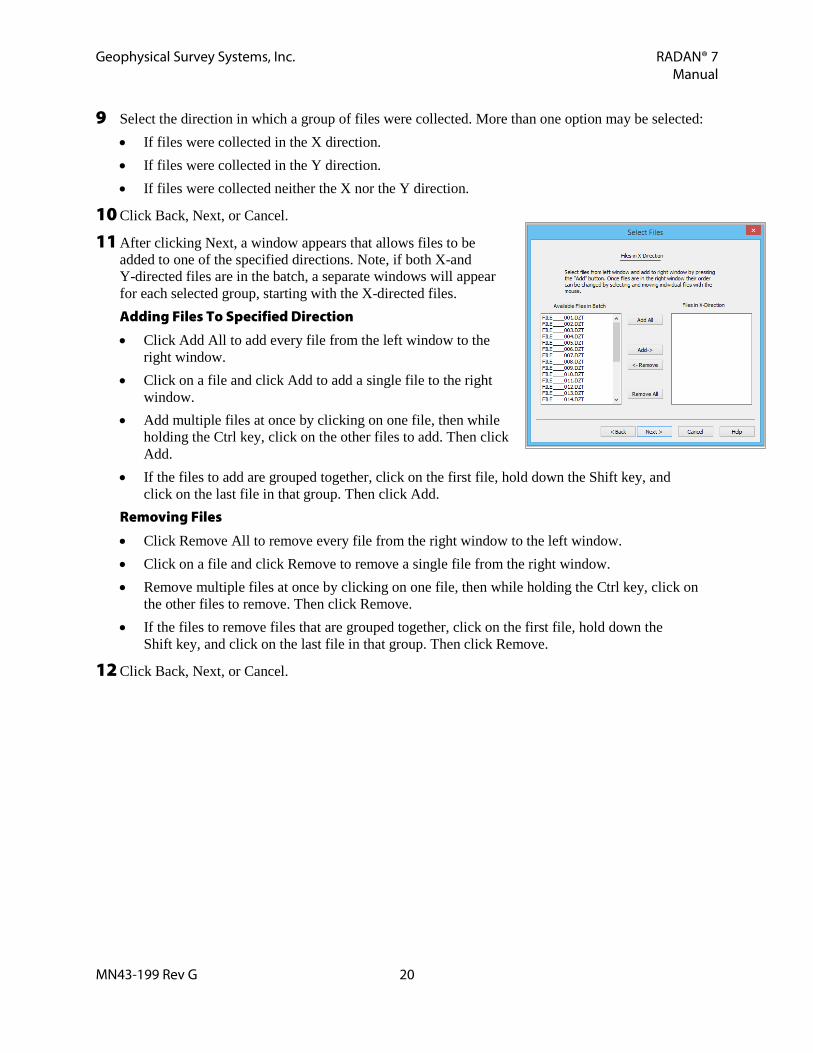
9 Select the direction in which a group of files were collected. More than one option may be selected: • If files were collected in the X direction. • If files were collected in the Y direction. • If files were collected neither the X nor the Y direction.
10 Click Back, Next, or Cancel.
11 After clicking Next, a window appears that allows files to be added to one of the specified directions. Note, if both X-and Y-directed files are in the batch, a separate windows will appear for each selected group, starting with the X-directed files. Adding Files To Specified Direction
• Click Add All to add every file from the left window to the right window.
• Click on a file and click Add to add a single file to the right window.
• Add multiple files at once by clicking on one file, then while holding the Ctrl key, click on the other files to add. Then click Add.
• If the files to add are grouped together, click on the first file, hold down the Shift key, and click on the last file in that group. Then click Add.
Removing Files
• Click Remove All to remove every file from the right window to the left window. • Click on a file and click Remove to remove a single file from the right window. • Remove multiple files at once by clicking on one file, then while holding the Ctrl key, click on
the other files to remove. Then click Remove. • If the files to remove files that are grouped together, click on the first file, hold down the
Shift key, and click on the last file in that group. Then click Remove.
12 Click Back, Next, or Cancel.

Geophysical Survey Systems, Inc. RADAN® 7 Manual
MN43-199 Rev G 21
Setting Data Collection Area and Line Order
1 Specify the data collection area by choosing the option “Use entire 3D display area selected earlier” or “Use Different 3D area”. If the second option is selected, enter in the minimum and maximum X- and Y- coordinates of the survey area for the specified line direction.
2 Click on the Down arrow next to the yellow orientation section. Select the direction and orientation for how the data were collected.
3 Click Back, Next, or Cancel.
4 If necessary, double-click on the individual files and input the starting and ending XY coordinates of that profile. • Enter starting and ending XY coordinates. • View File to view the individual file • Click OK.
5 Click Back, Next, or Cancel.
6 Lastly, input GPS coordinates for this grid if available.
7 Click Back, Finish, or Cancel.

Geophysical Survey Systems, Inc. RADAN® 7 Manual
MN43-199 Rev G 22
3D File This provides a way to combine individual data files (.dzt) that were collected in a grid format and assemble them together to create a 3D file. The information necessary to create the 3D file is stored in the Grid Project file (.m3d). Files collected can be collected in the X direction only, Y direction only, or both X and Y direction.
1 After selecting 3D File, enter a filename for the 3D Grid to create.
2 Click Save to continue.
3 3D Grid Options: Enter the following grid parameters based upon how the data were collected and will be combined into a 3D Grid file. • 3D Filename: This is the name of the single .dzt file that RADAN 7 will construct from the
individual profiles, and the location where it will be stored. Change either the name or the storage directory by clicking on this button.
• Files in X/Y Direction: If the same grid was collected twice, but with perpendicular transects, these tabs are used to define different input parameters for each direction. For example, data collected zig-zag in the X direction, but in the Y as unidirectional lines, are input as different line orders under each tab.
• Starting (units): This is the coordinate of the bottom left corner of the grid. If the smaller grid is tied into a larger site grid, input those coordinates here so that the axis of the resultant 3D file matches with the larger area.
• X-Length/Y-Length: These are the maximum coordinates of the grid. For example, if the grid is 100 inches × 100 inches, put those values in here. If the profile lines are not all the same length, put in the measurement of the longest one.
• # Profile Lines: Total number of lines in either the X or the Y direction.
• Line Spacing: This is the distance between each survey transect. The software figures out this number by dividing the grid size by the number of profile lines. Use this distance as error checking. If data were collected with transects placed one foot apart, and the number of transects for the grid size is accurate, then the line spacing should be 1. Anything else and there is a positioning error.
• Line Order: This is a pull down menu. Visualize the site grid and the order in which files were collected, and choose the orientation that best matches.
• Working Folder: This is where data are stored. Clicking this button will open a browser to select a different directory.
Note: Do not forget to count the “0” transect. If scanning a 10 × 10 foot area with profiles every one foot, and the first profile is at 0 and the last is at 10, there will be 11 profiles.

Geophysical Survey Systems, Inc. RADAN® 7 Manual
MN43-199 Rev G 23
• Auto Load Files: By checking this box, RADAN 7 will go to the working directory and automatically input the data files in alpha-numerical order. This is the same order that is shown when data files are sorted by name in Windows Explorer (by clicking on the Name column header). If the files are not in the correct naming convention, it may be easier to rename them in Windows Explorer.
4 After completing all the selections in the dialog, click OK to open the 3-D File Creation window.
5 The window shows the actual locations and orientations of the profiles. If “Auto Load Files…” was selected in 3D Grid Options the left pane will show a list of file names with starting and ending coordinates.
6 Existing filenames and coordinates can be edited two different ways. • Click on a filename located in the left pane.
Then double-click that filename to edit the coordinates. • Move the mouse cursor to a line located in the right pane
and click on it.
7 Delete a line by clicking on the file in the left pane and pressing the Delete key.
8 Add files to the grid by clicking Add File. Click Filename to browse and select the appropriate file. Then enter the X and Y starting and ending coordinates for that line. Click OK to save and continue. • The Skip Distance option skips a certain distance from the start of
the file when writing to the 3D output file. This is particularly beneficial for files that were mistakenly started with the antenna in back of the starting point for the grid.
• Use the Align File End button if files were collected in a Zig-Zag pattern. This button will adjust the file so that the last scan is aligned with the end of the grid. This option is typically used in cases where the user is more confident in the ending position of the profile than the starting position. This option is only available for evenly spaced x- or y-directed files.
9 Once satisfied with the look of the grid, click OK in the 3-D File Creation window and the software will combine all the files and create a single grid file.

Geophysical Survey Systems, Inc. RADAN® 7 Manual
MN43-199 Rev G 24
Super 3D File Combine multiple 3D Grids to create one “super” 3D Grid. This will create a new file with the extension .dzt. A separate created .s3d file, which contains the information used to create the output .dzt file is also created.
1 After selecting Super 3D File, enter a filename for the Super 3D file (.s3d) being created. Click Save to save and continue.
2 Click Add File to retrieve an already assembled 3D grid.
3 File Parameters: Populate the File Parameters window. • Filename: Click Filename to browse and retrieve a grid. • Starting (X,Y) Coords: Enter the X,Y position for this grid. • If this is the first grid being added, the Starting (X,Y)
coordinate is likely 0,0. • If necessary, Rotate, Flip Horizontally, and/or Flip Vertically,
depending on how the grid was collected relative to the coordinates of the first grid added. • Click OK the File Parameters are complete.
4 If there are more grids to add, continue back to step 1 and repeat.
5 Once all of the grids are added, click OK and the system will combine all the grids and create one 3D file.
Gridded 3D File This option takes one or more 3D files or files with GPS coordinates and creates a 3D gridded file. The gridded file is organized as a series of profiles oriented in the X-direction for local 3D coordinates and East-West direction for GPS coordinates. Access this option from the
Assemble Data Menu, which is accessible from the button when no files are open.
1 After selecting Gridded 3D File from the dropdown list, choose the folder containing the file(s) to be gridded. All files to be gridded must reside in the same folder.
2 Click Next to continue or Cancel to cancel the process.
3 There will be two panes: Available Files in Folder are files available to append; and Batch Files are the files that will be batched together. Add ALL files that should be included with the gridded 3D grid. Adding Files to be Gridded
• Click Add All to add every file from the left window to the right window. • Click on a file and click Add to add a single file to the right window. • Add multiple files at once by clicking on one file, then while holding the Ctrl key, click on the
other files to add. Then click Add.

Geophysical Survey Systems, Inc. RADAN® 7 Manual
MN43-199 Rev G 25
• If the files to add are grouped together, click on the first file, hold down the Shift key, and click on the last file in that group. Then click Add.
Removing Files
• Click Remove All to remove every file from the right window to the left window. • Click on a file and click Remove to remove a single file from the right window. • Remove multiple files at once by clicking on one file, then while holding the Ctrl key, click on
the other files to remove. Then click Remove. • If the files to remove files are grouped together, click on the first file, hold down the Shift key,
and click on the last file in that group. Then click Remove.
4 When files are added to the window above, a temporary file is created and the locations of the files in 3D space are indicated by the location view as seen in the image above.
5 Click Next to move to the next screen.
6 The next window that appears specifies the dimensions of the 3D gridded area. By default, the area that appears encompasses all the data. There is an option to change the area to grid a subset of the data in this window. If there are not GPS coordinates, the area coordinates will be the horizontal units (e.g. feet or meters).
7 Click Next to move to the next screen.
8 The next window that appears is used to specify gridding intervals and method. • Specify the distance between scans: Note how the gridded
file size changes when the interval is changed. This may dictate how fine a grid interval is possible.
• Specify neighbor search information: Four is the default value for nearest neighbors. The neighbor distance should be at least the separation distance between profile lines.
• Specify gridding method: The greater the Distance Power the less of an effect points farther from the grid node will have during interpolation. 1 is the default value and 3 is the maximum for RADAN 7.

Geophysical Survey Systems, Inc. RADAN® 7 Manual
MN43-199 Rev G 26
9 Click Finish to create the Gridded 3D File. A status bar will indicate the progress of the file being created.
10 Once the 3D gridded file is created, a prompt will appear to enter a file name. The file will open automatically after a name is provided.
Import GPS If data were collected using GPS and it wasn’t automatically imported when the .DZT file(s) were opened, select this option to import GPS data. First, open the GPR data file. Then click the Import GPS menu option. The GPS file name will default to the same file name of the data file, except the GPS file will have a .tmf extension if the data were collected with a SIR 20 or SIR 3000 and a .dzg extension if the data were collected with a more recent system (SIR 4000, SIR 30, UtilityScan DF).
Save This will save the current active file along with all the parameters of the file.
Save As Save the current active file as: RADAN File: Saves the file as the default .dzt file. RADAN File: Reversed: Reverses the direction of an individual .dzt file. RADAN File: Split Channels: When multi-channel data is collected this saves the data as separate single-channel output files. The original channels are designated by the letter appended to the input filename. For example, if the original 2-channel file is File_001.dzt, the output files will be File_001a.dzt and File001b.dzt, where the “a” denotes the original channel 1 data and “b” denotes original channel 2 data. RADAN File: Resampled: Resample the data currently open in RADAN 7. The resampling is performed on the samples/scan of the open file. SEGY File: Saves data as a .sgy file.

Geophysical Survey Systems, Inc. RADAN® 7 Manual
MN43-199 Rev G 27
Export Export the current active file as: • Picture as a JPG format (.jpg) • Picture as a Bitmap format (.bmp) • Picture as a PNG format (.png) • Custom Image: Opens a menu to select Image Type, Image Window, Image Size, and whether to split
the output into multiple files. One of the options is to export the entire file as a linescan image. • AutoCAD File (.dxf), which is a 2D CAD file. The 3D window must be open for this option to be
available. • 3D AutoCAD File (.dxf). The 3D window must be open for this option to be available. • Shape File (.shp). The 3D window must be open for this option to be available. • 3D Slice as ASCII format, Comma Delimited (.csv): Choose from saving with the displayed X, Y, or
Z slice as an ASCII csv file. The 3D window must be open for this option to be available. • Google Earth Format (.kml): Exports layers, targets, user marks, ground truth, and/or the GPS path
into a Google Earth .kml file that can be viewed in Google Earth when the file is opened in Google Earth.
• Z-slice Google Earth (.kml): Exports the Z-Slice to a Google Earth KML file that will be appear as an overlay in Google Earth when it is opened in Google Earth. The 3D window must be open for this option to be available.
• Picks (.csv): Opens a set of menus to export Targets or Layers. See Ribbons: Structure and Functions for more information on how to export Picks.
• File Header (.txt)
Print Print an image of the current active file. Quick Print: Print directly to the default printer. Setup: Enter print options such as Scan per Inch, Print Page Headers, Continuous Page, and a logo (Load Logo) or GSSI logo. Print Preview: Preview the output on the screen prior to printing. Print: Printer setting will display.
Close Click Close to close the active file.
Close All Open Files Click to close all of the open files.
Options Change languages.
Exit Click Exit to exit the software.
Geophysical Survey Systems, Inc. RADAN® 7 Manual
MN43-199 Rev G 28
Panes and Tables
My Files, Processes & Proc. List Pane
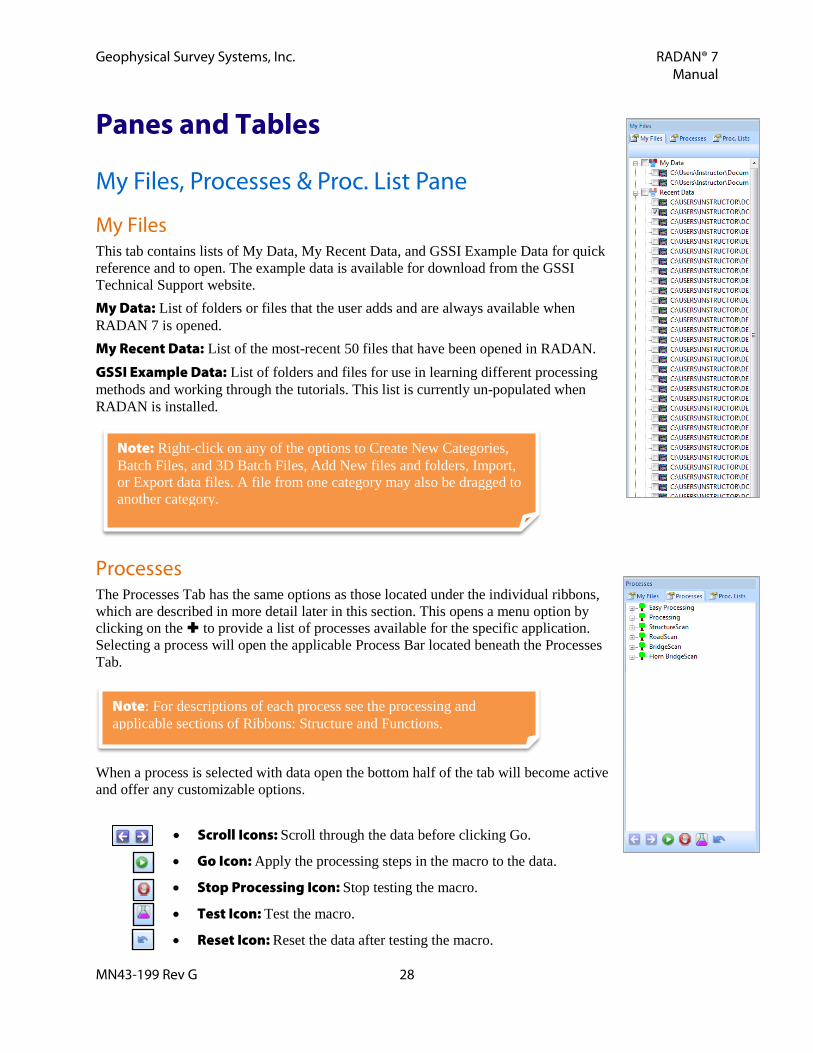
My Files This tab contains lists of My Data, My Recent Data, and GSSI Example Data for quick reference and to open. The example data is available for download from the GSSI Technical Support website. My Data: List of folders or files that the user adds and are always available when RADAN 7 is opened. My Recent Data: List of the most-recent 50 files that have been opened in RADAN. GSSI Example Data: List of folders and files for use in learning different processing methods and working through the tutorials. This list is currently un-populated when RADAN is installed.
Processes The Processes Tab has the same options as those located under the individual ribbons, which are described in more detail later in this section. This opens a menu option by clicking on the to provide a list of processes available for the specific application. Selecting a process will open the applicable Process Bar located beneath the Processes Tab. When a process is selected with data open the bottom half of the tab will become active and offer any customizable options.
• Scroll Icons: Scroll through the data before clicking Go.
• Go Icon: Apply the processing steps in the macro to the data.
• Stop Processing Icon: Stop testing the macro.
• Test Icon: Test the macro.
• Reset Icon: Reset the data after testing the macro.
Note: Right-click on any of the options to Create New Categories, Batch Files, and 3D Batch Files, Add New files and folders, Import, or Export data files. A file from one category may also be dragged to another category.
Note: For descriptions of each process see the processing and applicable sections of Ribbons: Structure and Functions.

Geophysical Survey Systems, Inc. RADAN® 7 Manual
MN43-199 Rev G 29
Proc. Lists With the Process List Tab selected choose from the following macros. A macro is a series of processing steps and/or options put together into one option. My Process List: List of processes (macros) the user creates for future use. Custom process lists can be created by right-clicking on the My Process Lists tree item and selecting New->Process List from the menus that appear. This will open a window that contains a process tree. A process list is created by selecting individual processes in the process tree, then pressing the Add -> button. After the desired processes are added, click on the OK button to add the newly-created process list to the My Process Lists tree. The My Process Lists tree item may have to be expanded to see the newly created process list. All Process lists are saved so that they are available the next time RADAN is run.
GSSI Process List: List of processes (macros) prepopulated for commonly used processes. The GSSI Process List is organized by application. Temporary Process List: List of processes (macros) created for temporary use that contain the process information generated on the data collection unit. Files which possess process lists include those collected with SIR 30, SIR 4000, and UtilityScan-DF files. When a process list is selected with data open the bottom half of the tab will become active and offer any customizable options.
• Scroll Icons: Scroll through the data before clicking Go.
• Go Icon: Apply the processing steps in the macro to the data.
• Stop Processing Icon: Stop testing the macro.
• Test Icon: Test the macro.
• Reset Icon: Reset the data after testing the macro.

Geophysical Survey Systems, Inc. RADAN® 7 Manual
MN43-199 Rev G 30
Properties Pane The Properties Pane will display one of four options; Global Settings, File Header, Window Settings, Data Channel Properties. The Properties Pane can be toggled On and Off from the Home Ribbon – Windows Group.
Global Settings Global Settings in the Properties Pane needs to be set prior to opening any data files. The Global Parameters are only accessible when there are no open files.
File Parameters Auto Save File:
• YES: Automatically saves processed files into a folder labeled Proc in the established Source Directory.
• NO: Prompts the user to save each processed file into an established Output Directory.
Source Directory: Select the folder where the source (original data is located). Output Directory: Select the folder where the processed data will be saved (only an option if Auto Save File is set to No).
View Attributes Display Channel: Select which channel to display/process if multiple channels are available. Marker Style: Select None, Long, or Short for the type of User/Distance marks to be displayed. The Long and Short options apply to the User Marks and the None option hides all the marks. Horiz. Scale:
• Show: Display horizontal scale. • Hide: Do not display horizontal scale.
Grid Lines:
• Show: Display horizontal grid lines. • Hide: Do not display horizontal grid lines.
Data Attributes When a file is opened, the scale will default to whatever units were saved with the file. Vertical Units: Units for the vertical scale. Horiz Units: Units for the horizontal scale. GPS Units: Units for GPS information displayed in the tables, status bar, and 3D window .
Note: Double-click on the left or right column to change/select options or click on either column and click on dots or down arrow to change/select options.
Note: Once a file is open the Global Parameters cannot be changed. All data files must be closed to make changes.

Geophysical Survey Systems, Inc. RADAN® 7 Manual
MN43-199 Rev G 31
Application-Specific Display Switch between displays that include processing and viewing options based on the selected application. Auto-Switch Display:
• No: Data will open in the currently selected display. • Yes: The display will change based on the data file opened. For
example, if data collected with the StructureScan Mini is opened while in the Standard Processing Display, the display will automatically switch to the RADAN 7 for StructureScan Mini display.
Current Display:
• Reader: Opens the RADAN Reader display, which allows you to view already processed 2D data as profiles and 3D data as depth slices. The color table, color transform, and display gain can also be modified. If targets or picks were added in one of the other displays they can be displayed as well. Displayed data can be saved as .jpg images. This display is available with any purchase of RADAN 7 and will become the only way of viewing data once the demo version of the software expires without activation.
• Standard Processing: This is the most inclusive display with access to all of the application-specific tabs as well as all 2D and 3D (with purchase of Interactive 3D Module) viewing and processing options.
• RADAN for StructureScan Mini: This is display that is designed specifically for data collected with the StructureScan Mini and includes the ability to instantly process data, do some additional processing, add interpretations, and export to a jpg or excel to quickly generate a report.
• UtilityScan DF: This is display that is designed specifically for data collected with the UtilityScan DF and includes the ability to instantly process data, do some additional processing, add interpretations, and export to a jpg or excel to quickly generate a report.
• RoadScan: Provides viewing and processing options for data collected specifically for determining pavement layer thickness.
• Ground-Coupled BridgeScan: This display is designed to process data specifically collected to determine bridge deterioration using a ground-coupled antenna.
• Horn BridgeScan: This display is designed to process data specifically collected to determine bridge deterioration using an air-launched horn antenna.
• Dual Pol. Horn BridgeScan: This display is designed to process data specifically collected to determine bridge deterioration using two air-launched horn antennas mounted at right-angles to one-another.

Geophysical Survey Systems, Inc. RADAN® 7 Manual
MN43-199 Rev G 32
File Header Once a file is open, Header information about the file will be displayed in the Properties Pane.
Header File Parameters Original File: Name of the original file. This will display the name of the original file even if a processed file is open. Created: Date the original file was created. Modified: Date the open file was last modified. Number of Channels: Number of channels the open files contains.
Horizontal Parameters Scans/Sec: Number of scans collected per second in the open file. Scans/unit: Number of scans collected per unit (meters, feet, etc.) in the open file. This number can be modified. Units/Mark: Number of units (meters, feet, etc.) collected per mark. This number can be modified.
Vertical Parameters Samples/Scan: Number of samples collected per scan. Bits/Sample: Number of bits per sample. Dielectric Constant: Dielectric value entered when the data were collected. This number can be modified and also controls the calculated vertical depth scale in the linescan and wiggle windows.
Channel Information Channel: Which channel to display in Header Information. Antenna Type: Antenna frequency used to collect the data. Antenna Serial #: Serial number of the antenna used to collect the data if available. Position (ns): Position of the start of the scan (Time-Zero) used when collecting the data. Range (ns): Range of the data (depth) in time used to collect the data. Top Surface: Height of the scan above the direct wave, i.e. above ground surface, from when the data were collected. This will typically be a negative number. Depth: Maximum depth range calculated based on the Range and Dielectric set during field collection. Processing History: Processing steps and the order in which they occurred are recorded here. Below are examples of the processing steps displayed.
• IIR Filters: IIR filters applied to the data. • FIR Filter: FIR filters applied to the data. • Position Correction: Time Zero processing. • Range Gain: Any Gain modifications. • Background Removal: Background Removal applied.

Geophysical Survey Systems, Inc. RADAN® 7 Manual
MN43-199 Rev G 33
Window Settings Once a file is open, how the information is displayed can be viewed and changed. The Properties Pane automatically updates based on which data display, 2D or 3D is currently selected.
View Attributes (2D & 3D) Display Channel: Display all channels or a specific channel. Marker Style: Change mark lines to display as either None, Short, or Long. Grid Lines: Hide or Show 3D grid lines.
Data Attributes (2D & 3D) Use Surface: Yes or No. This aligns time-zero with the top of the display. Hide Blank Data: Yes or No. Hides portion of scans with zeroed-data obtained from position shifting. Start Sample: Starting sample to display data. This will default to the sample corresponding to time-zero when Use Surface is set to Yes. End Sample: Ending sample to display data. This will default to show the last valid sample number.
Application-Specific Display (2D or 3D) Switch between displays that include processing and viewing options based on the selected application. Auto-Switch Display:
• No: Data will open in the currently selected display. • Yes: The display will change based on the data file opened. For example, if data collected with
the StructureScan Mini is opened while in the Standard Processing Display, the display will automatically switch to the RADAN 7 for StructureScan Mini display.
Current Display:
• Reader: Opens the RADAN Reader display, which allows you to view already processed 2D data as profiles and 3D data as depth slices. The color table, color transform, and display gain can also be modified. If targets or picks were added in one of the other displays they can be displayed as well. Displayed data can be saved as .jpg images. This display is available with any purchase of RADAN 7 and will become the only way of viewing data once the demo version of the software expires without activation.
• Standard Processing: This is the most inclusive display with access to all of the application-specific tabs as well as all 2D and 3D (with purchase of Interactive 3D Module) viewing and processing options.
• RADAN for StructureScan Mini: This is display that is designed specifically for data collected with the StructureScan Mini and includes the ability to instantly process data, do some additional processing, add interpretations, and export to a jpg or excel to quickly generate a report.
• UtilityScan DF: This is display that is designed specifically for data collected with the UtilityScan DF and includes the ability to instantly process data, do some additional processing, add interpretations, and export to a jpg or excel to quickly generate a report.

Geophysical Survey Systems, Inc. RADAN® 7 Manual
MN43-199 Rev G 34
• RoadScan: Provides viewing and processing options for data collected specifically for determining pavement layer thickness.
• Ground-Coupled BridgeScan: This display is designed to process data specifically collected to determine bridge deterioration using a ground-coupled antenna.
• Horn BridgeScan: This display is designed to process data specifically collected to determine bridge deterioration using an air-launched horn antenna.
• Dual Pol. Horn BridgeScan: This display is designed to process data specifically collected to determine bridge deterioration using two air-launched horn antennas mounted at right-angles to one-another.
O-scope Parameters (2D w/Scope Selected from Data Windows Group) Color: Change the color of the wiggle trace.
Wiggle Parameters (2D w/Wiggle Selected from Data Windows Group) Chop: Show Both, Show Positive, or Show Negative. Removes the peaks in the specified direction. Fill: None, Positive, or Negative. Fills in the peaks of the wiggle traces. Fill Level: Fills in a percentage of the upper peaks. Scale: Sets the amplitude scale. Skip: Skips a specified number of scans. Stack: Stacks a specified number of scans per wiggle trace. Space: Changes the spacing between individual wiggle traces. Line Width: Line width of wiggle trace in pixels. Color: Change the color of the wiggle traces.
XYZ Slicing (3D) X Position: The position of the X-Slice in the 3D volume. Y Position: The position of the Y-Slice in the 3D volume. Z Position: The position of the Z-Slice in the 3D volume.
Z Slice Options Thickness As: Slice Thickness in either Depth, Samples, or Time. Thickness: Thickness of the Z Slice. One-half of the slice thickness extends ½ above the slice position and ½ below the slice position. 3D Z Slice Mode: Toggle between On/Off to give the Z Slice a “3D” look.

Geophysical Survey Systems, Inc. RADAN® 7 Manual
MN43-199 Rev G 35
XYZ Visibility Section: Toggle On/Off a blocked cube image. Transparency: Only show a percentage of the positive amplitude reflections from a range of Z slices. See Through: Only show the positive amplitude reflections from one Z slice. Snaps: When animating or scrolling through any slice can choose to snap the slice to the profiles actually collected. X, Y, Z: Toggle On/Off X, Y, Z slices. X Data: Show/Hide data obtained from profiles oriented in the X-direction. Y Data: Show/Hide data obtained from profiles oriented in the Y-direction. Other Data: Show/Hide data obtained from profiles that are not oriented in the X-direction nor the Y-direction.
Z Slice Processing Max RMS: The Z slice will show either the maximum value or the root mean squared value. Using either will smooth the data. Bkg Removal: Toggle between On/Off to remove background from the Z slice. Horizontal Smoothing: None, 1, 2, or 3. 1, 2, and 3 correspond to 4, 8, and 16 samples used in a 2D moving average on each side of a data point (i.e. sample). The 2D area is a square if the data density is the same in both directions, and padded on the edges of a 3D area by mirroring the data before applying the moving average. If the actual spacing between the data points used to construct the slice is different in the x- and y-directions, then the maximum dimension of the moving average window is the value indicated by the filter (4, 8, or 16 data points), and therefore the other dimension of the window is rounded to the nearest even integer value. For this scenario the 2D moving average operating on the slice is a rectangle instead of a square.
3D Toggles Points: Toggle Show/Hide points or dots. Unlinked targets will be shown or hidden by toggling this button. Lines: Toggle Show/Hide lines, i.e. rebar or pipes. Linked targets will be shown or hidden by toggling this button. Contour: Toggle Show/Hide Z slice contour. Surfaces: Toggle Show/Hide surfaces. Surfaces are obtained by loading a .shp file created in RADAN 6.

Geophysical Survey Systems, Inc. RADAN® 7 Manual
MN43-199 Rev G 36
3D Style Grid: Toggle Show/Hide Grid. Minor Grid X, Y, Z: Adjust the number of grid lines in each axis. Mesh: Toggle Show/Hide Mesh. Background: Change the background between Black or White. Lock Aspect Ratio: Toggle On/Off Lock Aspect Ratio. Locking the aspect ratio keeps the target dimensions from being stretched when the 3D volume dimensions are stretched or compressed in the X-, Y-, or Z-directions. Open Shape Files: Opens a .shp file created in RADAN 6.
Data Channel Properties Once a file is open, information about the antennas used to collect the data can be displayed. If only one antenna was used to collect the data, only Channel 1 Properties will be visible. This information is modifiable.
Channel # Properties Antenna Gain Adjustment: Antenna-specific gain can be applied. This gain is independent of the display gain and is useful for balancing the gain between channels when viewing a multiple channel file. Display Gain: Display Gain of the currently selected channel of data. Inline Offset: Offset of the antenna in the direction of travel from a reference point. Typically this is the offset from a GPS location. For multiple channel data obtained without a GPS, this value can be used as the position of the antenna relative to a fixed point on the data collection vehicle or cart. Inline offset is positive in the forward direction of travel. CrossLine Offset: Offset of the antenna perpendicular to the direction of travel. A positive offset would be to the left of the antenna position Antenna Model: The GSSI antenna model number. Center Frequency: The center frequency of the antenna in MHz. Bistatic Separation: The distance between transmitting and receiving antennas.

Geophysical Survey Systems, Inc. RADAN® 7 Manual
MN43-199 Rev G 37
Table Pane This pane will display database information about the currently active file. Tabs are displayed depending on the type of application or process underway.
General Options Way Points: Computer generated or User generated User or Distance marks. These can be added or deleted in the table. Notes: Enter notes about the file. This is also the location of notes that are recorded with the file on SIR 20 units. Way Point Names: The list of names created when populating the Way Points tab with Way Point Names. Channel Positions: For multi-channel files, this is the offset information for each channel relative to a fixed location. For data obtained with GPS, the fixed location is typically the location of the GPS antenna. See descriptions of Inline and Crossline Offset in Data Channel Properties description in previous section. Profiles: The profile location information is presented in this table. Profile starting distances and the direction of counting (upward or downward) are shown as editable entries in the table. For files containing multiple profiles, such as 3D files and batch files, there will be a row in the table for each profile. The 3D coordinates of the profiles may be modified by clicking on Edit 3D Position button in the far right of each row. Velocity Analysis: Details generated when a Velocity Analysis is performed under the Focus Group of the Processing Ribbon. 3D SubArea Options: Contains options that are useful when viewing Super-3D files containing multiple subareas. Formerly, in RADAN 6, these subareas were called Regions. There will be a row in the table for each subarea. Many of these parameters are also useful for regular 3D files. Name: The name of the subarea. For certain 3D files this will be blank by default. This is an editable column. X St, X End, Y St, Y End: Outer coordinates of 3D subarea that are shown in the 3D volume. These values can be edited by pressing the Edit 3D Display Area button on the far right column of the row. Rot. Ang. (CCW): Counter-clockwise rotation angle of the subarea in local coordinates. The origin of rotation will be the minimum (x,y) coordinates of the 3D area. X Data: Show/Hide data obtained from profiles oriented in the X-direction. Y Data: Show/Hide data obtained from profiles oriented in the Y-direction. Other Data: Show/Hide data obtained from profiles that are not oriented in the X-direction nor the Y-direction. Hide: Show/Hide subarea data. This may be useful when dealing with multiple overlapping subareas in a Super-3D file. Loc. 3D Gain: Local Gain value, in decibels, applied to the 3D subarea. This is useful to balance the gains between multiple subareas in a Super-3D file. Display Order: The order in which the subareas are displayed in the Z-slice when there are multiple overlapping subareas. The lower number is on top.

Geophysical Survey Systems, Inc. RADAN® 7 Manual
MN43-199 Rev G 38
Edit 3D Display Area: This is a button that opens a window that allows the user to edit the position of the 3D volume in local 3D coordinates.
Target Options Define how each target is displayed and behaves. Target Ground Truth: Details about each target that is corrected for depth using Ground Truth in Interactive Mode. Target Picks: Details about each individual target added using Interactive Mode. Targets: Details about the target Focus groups. Each target group may have one or more target picks.
Layer Options Define how each layer is displayed and behaves. Layer Depths: Layer depths listed by scan. Layer Ground Truth: Details about each layer that is corrected for depth using Ground Truth in Interactive Mode. This is organized by scan. Layer Pick Details: Details about each individual layer added using Interactive Mode. Layers: Details about the layer Focus groups.

Geophysical Survey Systems, Inc. RADAN® 7 Manual
MN43-199 Rev G 39
Ribbons: Structure and Functions The Ribbon contains options to process the data, different ways to display the data, and processing options specific to specialized applications. Each tab in the Ribbon contains these different options.
Home Ribbon
File Group Open: Opens the currently selected project folder to open additional files. Save: Saves the selected data file. If multiple files are open it saves the tab that is active. Any new targets or picks added to the data will be saved. Close: Closes the currently selected data file. If multiple files are open it closes the tab that is active.
Data Window Group LineScan In the linescan display data are displayed in a color-amplitude form, where a color is assigned to a specific positive or negative amplitude value of the recorded signal dependent upon the color table and color transform selected. The vertical scale represents time (or depth) while the horizontal scale represents the horizontal distance traveled by the radar antenna. The Linescan display is the most useful for mapping man-made objects, such as underground storage tanks, pipes, and drums or for mapping geologic layers. Scope This will display an O-Scope to the right of the linescan data. Hold the left mouse button down while pointing to the linescan data to correspond the same point with the O-Scope using a horizontal line. 3D View This will display the data as a 3D Cube. More information and options on this mode are discussed in the Basic Processing/Tutorials section under Basic 3D Grid Navigation.

Geophysical Survey Systems, Inc. RADAN® 7 Manual
MN43-199 Rev G 40
Wiggle This display shows individual scan traces. The settings for this display can be changed in the Properties Pane.
Location Used primarily for 3D Grid files or individual profiles with GPS data, location will display a grid showing the location of each profile.
• Holding the left mouse button down on the linescan data will show the location of that spot on the location display.
• Right-click with the mouse inside of the location display to access the following: o Move 3D Area: Change the starting coordinates of the grid. o GPS Coordinates: Add or modify the GPS Coordinates for the grid.
• Right-click with the mouse on the end of a line to access the following: o Nudge Profile: Shift the profile forward or backward along the line. o Edit Profile Coordinates: Change a profile’s location within the grid.
Depth Pane: Toggles the Interactive Interpretation Pane On or Off below the linescan display.
Other Windows Toggle On or Off different data property windows. My Files: This tab contains lists of My Data, My Recent Data, and GSSI Example Data for quick reference and to open. The example data is available for download from the GSSI Technical Support website. Processes: The Processes Tab has the same options as those located under the individual ribbons, which are described in more detail later in this section. This opens a menu option by clicking on the + and then selecting which processing steps to apply. Selecting a step will open the applicable Process Bar located beneath the Processes Tab. Process Lists: Opens a list of macros available for data processing. Tables: This pane will display database information about the currently active file. Tabs are displayed depending on the type of application or process underway. File Header: Header information about the displayed file. Window Settings: The Properties Pane automatically updates based on which data display, 2D or 3D is currently selected. Data Channel Properties: Shows channel information for the selected data. Datasets with multiple channels will display individual properties for each channel. Global Settings: Display Global Parameters for all files in a particular project prior to opening any files and allow you to switch between available Application Displays. Once a file is open, the Global Parameters cannot be changed.

Geophysical Survey Systems, Inc. RADAN® 7 Manual
MN43-199 Rev G 41
Display Group Color Tables Color tables are used to code the amplitude of each scan (i.e., the recorded radar signal). Colors on the left side of the spectrum represent strong negative amplitudes. As the colors go to the right, this represents the amplitude getting weaker (or closer to 0) and the middle of the spectrum is the area of weak amplitude. As the colors go further right from the middle, this represents a stronger positive amplitude. • For example, white in color table 1 corresponds to the highest positive amplitude
pulse; therefore, when it appears on the radar record, it means that there is a strong reflection (or a high dielectric contrast).
• In some color tables (such as 23), black indicates a low amplitude reflection. Therefore, a large black region on the linescan plot could be indicative of a uniform structure (such as a homogeneous sand deposit) with little or no dielectric contrast.
Color Xforms The Color Transform can be changed to enhance weak amplitude or small contrast reflectors. The color transform determines whether the color scale applied to the radar wave’s amplitude is linear, logarithmic, exponential, or customized. This function can also be used to de-emphasize certain features.
Display Gain To change the Display Gain, click Display Gain in the Home Ribbon or right-click on the data window and select Display Gain. Then select from a preset list of multiples ranging from -6 up to 60. Input a Custom Value by right-clicking and selecting Custom from Display Gain menu. This will change all samples, no matter where they are in the scan trace, by the same amount.
• Altering the display gain does not change data values like Range Gain, which is described later in this section under the Easy Processing and Processing sections.
• Altering the display gain may make it easier to see lower amplitude targets. Transfer Transfer is accessed through the Home Ribbon or by right-clicking on the data and has three options for changing how the data are displayed.
• Abs: Shows the absolute value of the data (all positive peaks). • Negate: Flips positive and negative peaks. • Spectrum: The displayed scan will be replaced with its frequency spectrum plotted in terms of
relative amplitude (0 to 1) versus frequency in MHz. Show This toggles the display of any targets or layers On or Off in the linescan and 3D-View.
Note: There are 30 different color tables and RADAN defaults to True Grey 17. There are 20 color transforms and
RADAN defaults to Linear Transform 3.
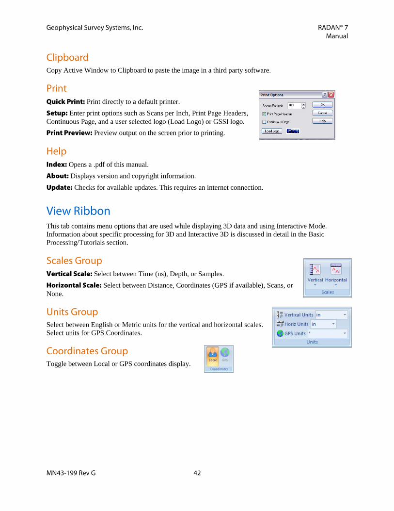
Geophysical Survey Systems, Inc. RADAN® 7 Manual
MN43-199 Rev G 42
Clipboard Copy Active Window to Clipboard to paste the image in a third party software.
Print Quick Print: Print directly to a default printer. Setup: Enter print options such as Scans per Inch, Print Page Headers, Continuous Page, and a user selected logo (Load Logo) or GSSI logo. Print Preview: Preview output on the screen prior to printing.
Help Index: Opens a .pdf of this manual. About: Displays version and copyright information. Update: Checks for available updates. This requires an internet connection.
View Ribbon This tab contains menu options that are used while displaying 3D data and using Interactive Mode. Information about specific processing for 3D and Interactive 3D is discussed in detail in the Basic Processing/Tutorials section.
Scales Group Vertical Scale: Select between Time (ns), Depth, or Samples. Horizontal Scale: Select between Distance, Coordinates (GPS if available), Scans, or None.
Units Group Select between English or Metric units for the vertical and horizontal scales. Select units for GPS Coordinates.
Coordinates Group Toggle between Local or GPS coordinates display.

Geophysical Survey Systems, Inc. RADAN® 7 Manual
MN43-199 Rev G 43
Easy Processing Ribbon This ribbon provides options to easily process data. Primarily, this is meant for data collected using Concrete Scan, UtilityScan, StructureScan Mini, or Palm Antenna.
Easy Fix – All In One This option goes through data processing step by step. Selecting Easy Fix will open a Temporary Process List in the My Files/Processes/Proc. List Tab Pane. The steps will guide the user through Time Zero, Background Removal, and Migration. All these steps are customizable or offer default settings where applicable. For more information about each processing step see the descriptions below.
Time Zero – Step 1 Sometimes it is necessary to vertically adjust the position of the whole profile in the data window. This is called Time Zero Correction. A corrected Time Zero provides a more accurate depth calculation because it sets the top of the scan to a close approximation of the ground surface. Follow the steps below to correct Time Zero for a ground coupled, bistatic antenna.
1 Click the Time Zero icon. This will display the Time Zero Process Bar in the left pane.
2 Position Correction Methods: There are six methods available to correct Time Zero. • Manual – User Estimates Peaks: Position the first positive peak of the direct
wave (the first reflection visible on the O-scope) by clicking on the O-scope with the left mouse button and dragging it up to the 0.0 line. This will adjust ground surface to appear at the top of the Data Pane window.
• Automatic: RADAN 7 will set the position of the first positive peak of the direct wave.
• Scan by Scan: Position correction for each scan individually. • H. Drift Tracking: Uses an algorithm to correct for any slight shifts in signal
position. • H. MiniTrack: Position correction for each scan of MiniSIR data.
Data Before Time Zero is Corrected
Data After Time Zero is Corrected

Geophysical Survey Systems, Inc. RADAN® 7 Manual
MN43-199 Rev G 44
• H. Thresh Tracking: Position correction for each scan by first positive or negative peak.
3 Click Apply to test the new position and, if necessary, click Reset and re-adjust.
4 Click OK once satisfied to process the data with the Time Zero correction.
Background Removal – Step 2 Background Removal is a filter, formally called a Horizontal Background Removal FIR Filter, which removes horizontal bands of noise similar to those seen in the image below. Sometimes these bands are caused by ‘real’ horizontal reflectors, but they can also be caused by low frequency noise such as antenna ringing. These layers can obscure other ‘real’ horizontal or point source reflectors. The maximum value for a Background Removal filter is 20001 scans. Filter length should be set to the number of scans equal to the feature length being removed. Any continuous feature within the data, such as a water table reflector or a stratigraphic boundary between two soil types, may also be filtered out by performing Background Removal. Be careful to not filter out desired reflectors.
1 Click the Background Removal icon. This will display the Background Removal Process Bar in the left pane.
2 Click BR Type to choose the type of Background Removal filter. • Full Pass: Will remove the horizontal noise throughout the enter profile. • Scan Range: Will remove the horizontal noise within specific scans.
Locate the beginning and ending scans by clicking the left mouse button on a linescan and looking at the scan number shown at the very bottom of the RADAN 7 window. o Start Scan: Enter the starting scan number where the horizontal noise
begins. o End Scan: Enter the ending scan number where the horizontal noise
ends.
Horizontal Noise to be Removed
Note: The Manual method of Time Zero Position Correction is recommended for most applications.
Note: This filter will remove the surface reflection (direct coupling) pulse. Therefore it should be performed following Time Zero Correction.

Geophysical Survey Systems, Inc. RADAN® 7 Manual
MN43-199 Rev G 45
• Adaptive BR: Length of the Background Removal filter is set automatically.
3 Click Apply to test Background Removal and, if necessary, click Reset and re-adjust.
4 Once satisfied with the Background Removal, click OK.
Test/Apply Filters – Step 3 This option offers multiple data filters. FIR filters have a finite-duration impulse response and, when encountering a feature in the data, are guaranteed to output a finite filtered version of that feature. This property makes it possible to design filters that are perfectly symmetrical and have linear phase characteristics. FIR filters will therefore produce symmetrical results so reflections will not be shifted in time or position. Refer to the Basic Processing/Tutorials section for more information on applying filters. There are three types of FIR filters available in RADAN 7, Boxcar Filter, Triangular Filter, and Custom Filter. Due to the symmetrical nature of FIR filters, FIR filter lengths should always be an odd number.
• Boxcar Filter: The Boxcar Filter is a rectangular filter window that performs a simple running average on the data. A portion of the data, determined by the filter length, is averaged, and the average is output as a single point at the center of the active portion of the filter window. The filter moves on to the next sample and the process is repeated. The Boxcar filter assigns equal weight to the data all along the filter length.
• Triangular Filter: The Triangular Filter emphasizes the center of the filter more heavily than the ends of the filter. This type of filter is a weighted moving average, with the weighting function shaped like a triangle. A portion of the data, determined by the filter length, is multiplied and summed by this function. The result is output at the center of the triangle. The filter then advances one sample and the process repeats.
• Custom Filter: This filter is only available for the Air Launched Horn Antennas that come with custom filters.
The user can also choose to filter either horizontally or vertically. Horizontal filters include Background Removal and Stacking. Vertical filters include Low Pass and High Pass Frequency Filtering.
• Background Removal Horizontal Filter: This filter is the best way to remove horizontal bands of noise. The length of the filter should always be a greater number of scans than the length in scans of the longest horizontal “real” reflector to be kept in the data.
• Stacking Horizontal Filter: Applies a simple running-average to stack the data. Stacking combines the adjacent selected radar scans and outputs a single scan. When stacking values are used in RADAN 7, the program will retain the marks in the file. However, the scans per unit distance and marks per unit distance will be changed in the header. For example, if there is a raw file with 80 scans per meter and 1 meter per mark and it is stacked by a factor of two (2) the output file would have 40 scans per meter written into the header (reduced by a factor of 2).
• Vertical Low Pass Filter: This filter will eliminate high frequency noise that often is seen in relatively deep radar profiles. It will reject frequencies below an established threshold. To identify the threshold it is recommended to view the Linescan data as a frequency spectrum. It is a good idea to reject all frequencies below the range where meaningful data are observed. Meaningful data is often estimated as being less than 2 times the center frequency of the antenna (i.e. less than 800 MHz for a 400 MHz antenna).
Note: Since the Triangular FIR Filter gives more weight to the center sample it is considered to be the filter that maintains more of the data integrity.
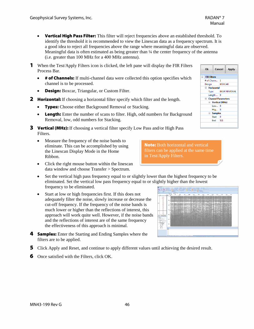
Geophysical Survey Systems, Inc. RADAN® 7 Manual
MN43-199 Rev G 46
• Vertical High Pass Filter: This filter will reject frequencies above an established threshold. To identify the threshold it is recommended to view the Linescan data as a frequency spectrum. It is a good idea to reject all frequencies above the range where meaningful data are observed. Meaningful data is often estimated as being greater than ¼ the center frequency of the antenna (i.e. greater than 100 MHz for a 400 MHz antenna).
1 When the Test/Apply Filters icon is clicked, the left pane will display the FIR Filters Process Bar. • # of Channels: If multi-channel data were collected this option specifies which
channel is to be processed. • Design: Boxcar, Triangular, or Custom Filter.
2 Horizontal: If choosing a horizontal filter specify which filter and the length. • Types: Choose either Background Removal or Stacking. • Length: Enter the number of scans to filter. High, odd numbers for Background
Removal, low, odd numbers for Stacking.
3 Vertical (MHz): If choosing a vertical filter specify Low Pass and/or High Pass Filters. • Measure the frequency of the noise bands to
eliminate. This can be accomplished by using the Linescan Display Mode in the Home Ribbon.
• Click the right mouse button within the linescan data window and choose Transfer > Spectrum.
• Set the vertical high pass frequency equal to or slightly lower than the highest frequency to be eliminated. Set the vertical low pass frequency equal to or slightly higher than the lowest frequency to be eliminated.
• Start at low or high frequencies first. If this does not adequately filter the noise, slowly increase or decrease the cut-off frequency. If the frequency of the noise bands is much lower or higher than the reflections of interest, this approach will work quite well. However, if the noise bands and the reflections of interest are of the same frequency the effectiveness of this approach is minimal.
4 Samples: Enter the Starting and Ending Samples where the filters are to be applied.
5 Click Apply and Reset, and continue to apply different values until achieving the desired result.
6 Once satisfied with the Filters, click OK.
Note: Both horizontal and vertical filters can be applied at the same time in Test/Apply Filters.

Geophysical Survey Systems, Inc. RADAN® 7 Manual
MN43-199 Rev G 47
Migration – Step 4 The radar antenna radiates energy with a wide beamwidth pattern such that objects several feet away may be detected. As a consequence of this, objects of finite dimensions may appear as hyperbolic reflectors as the antenna detects the object from far off and is moved over and past it. Deeper objects may be obscured by numerous shallower objects that appear as constructively interfering hyperbolic reflectors. Steeply dipping surfaces will also cause diffracted reflections of radar energy. This diffracted energy can mask other reflections of interest and cause misinterpretation of the size and geometry of subsurface objects. The apparent geometry of steeply dipping layers are an illusion and can be corrected in many cases. Migration is a technique that moves dipping reflectors, which appear as hyperbolic tails, to their true subsurface positions and collapses hyperbolic diffractions. There are two Migration methods available in RADAN 7: Hyperbolic Summation and Kirchhoff Migration.
• Hyperbolic Summation: Hyperbolic Summation works by summing along a hyperbola placed on the data, and placing the resulting average at the apex of the hyperbola. This process is repeated with the apex on every point in the data.
• Kirchhoff (default): The Kirchhoff Migration method is more accurate than the Hyperbolic Summation. An average value is still derived by summing along a hyperbola placed on the data and placed at the apex. However, Kirchhoff Migration also applies a correction factor to this averaged value, based upon the angle of incidence and distance to the feature. It also applies a filter to compensate for the summation process. This filter improves resolution by emphasizing the higher frequencies and applying a phase correction.
Migration can only be performed if there is at least one point-source hyperbolic reflector in the data. If a survey wheel was not used during data collection the data will first need to undergo Distance Normalization. More information about Distance Normalization can be found in the Processing section under Ribbons: Structure and Functions. The following file header parameters must also be assigned a value before the data can be migrated.
• Samples/scan • Range (ns) • Scans/unit
1 When the Migration icon is clicked, the left pane will display the Migration Process Bar and a Ghost Hyperbola will appear on the left side of the linescan.
2 Method: Choose either Kirchhoff Migration (default) or Hyperbolic Summation.
3 Hyperbola Fitting: Both the Hyperbolic Summation and Kirchhoff Migration require that the hyperbolic width and relative velocity are specified. Use the shape of the Ghost Hyperbola to fit over the top of the real hyperbola in the data. Notice that as the shape of the hyperbola changes, so does the velocity. The Ghost Hyperbola is a tool to help identify the correct velocity of the material that the electromagnetic energy is passing through. There are two ways to change the shape of the Ghost Hyperbola.
4 Process Pane: Move the square to adjust the shape of the Ghost Hyperbola.
5 Linescan: Reshape the Ghost Hyperbola using the three boxes that appear on the data. Once the Ghost Hyperbola matches the real hyperbola adjust the two vertical lines to mark the edges of the hyperbolic dipping reflectors to be summed. This is shown in the image below.

Geophysical Survey Systems, Inc. RADAN® 7 Manual
MN43-199 Rev G 48
6 As the Ghost Hyperbola is formed to fit over the real hyperbola notice how the velocity, dielectric, time (nS), and width all change. • Velocity: The speed at which the radar pulses travel through a material. The relative velocity is
the ratio between the length of a hyperbolic reflector in the distance axis (in number of scans/unit) to its length in the time axis on the screen (number of samples/unit).
• Dielectric: The relative dielectric permittivity is a dimensionless measure of the capacity of a material to store a charge when an electric field is applied. The dielectric constant is the real part of dielectric permittivity, as it is normalized to air. Dielectric constant values vary from material to material.
• Time (nS): This adjusts as the peak of the Ghost Hyperbola is positioned over the top of real hyperbolic reflector. This represents the two way travel time to the top of the reflector and is used to compute velocity.
• Width: Measured in number of scans, this is used to sum across the data file. This value should be set to about the same number of scans as the diffraction hyperbolas in the data. Larger values tend to give more accurate results, but if the value is too large, deterioration will occur.
• Gain: This function under the Migration Process Pane is used to increase the data amplitudes after migration, since migration usually reduces the amplitude of the radar signal. The Gain is usually set to a value between 1.5 and 5.
7 The following settings are not automatically updated, but can affect how Migration is performed and visualized. • Bistatic Offset: The distance between the transmitting and receiving antennas if using bistatic
antennas. • Load Vel(ocity) File: Open a .VLC file created during the Velocity Analysis Process (described
later in this section). • Minimum Plot Velocity: This is the minimum velocity displayed in the Velocity Plot. Adjust
this value to improve the display of the velocity in the plot. • Maximum Plot Velocity: This is the maximum velocity displayed in the Velocity Plot. Adjust
this value to improve the display of the velocity in the plot.

Geophysical Survey Systems, Inc. RADAN® 7 Manual
MN43-199 Rev G 49
8 Variable Migration: If multiple hyperbolas are available at different depths a variable migration can be performed on the data. • Select the shallowest hyperbola first and do a regular hyperbola fitting. • Double-click in the Velocity Plot to add a second box. This will create a new ghost hyperbola to
fit over another hyperbolic target. Perform a hyperbola fitting on the second hyperbola. • Continue to double-click creating additional boxes and
performing hyperbola fitting.
9 Click Apply to Test the Migration and, if necessary, click Reset and re-adjust. The Ghost Hyperbola was a good fit if the dipping sides of the reflector are removed as seen in the image to the right.
10 Once satisfied with the Migration, click OK.
Auto Target – Automated Process If data were collected using GSSI’s Structure Scan Mini, this option will automatically pick targets by placing Dots on the apex’s of the hyperbolic reflections. Each of the Dots will appear as in the Targets Tab as a separate target. The Target Picks tab will have all of the depth and velocity information for each of the Dots.
Max Depth – Automated Process This function analyzes the noise and signal loss (attenuation) from scan to scan and provides estimate of the effective depth penetration. Real reflectors may still be located beneath the Max Depth if they are strong enough. The output of this function is shown as a green line on the screen, as seen below, and saved as a .BII binary file.
1 When the Max Depth icon is clicked, the left pane will display the Max Depth Process Bar.
2 Max Depth Estimator: If multiple channels of data were collected, choose between which channels to use to estimate max depth.
3 Simply click Apply and Reset to test this processing function. Click OK to accept the setting and generate the binary file.
Note: It is recommended to change the color palette prior to performing Migration in order to see the Ghost Hyperbola clearly.

Geophysical Survey Systems, Inc. RADAN® 7 Manual
MN43-199 Rev G 50
Processing Ribbon This ribbon provides both standard and advanced processing of any data and for any application. It includes all of the same processing options from the Easy Processing Ribbon and more.
Time Zero Sometimes it is necessary to vertically adjust the position of the whole profile in the data window. This is called Time Zero Correction. A corrected Time Zero will provide a more accurate depth calculation because it sets the top of the scan to a close approximation of the ground surface. Follow the steps below to correct Time Zero for a ground coupled, bistatic antenna.
1 Click the Time Zero icon. This will display the Time Zero Process Bar in the left pane.
2 Position Correction Methods: There are six methods available to correct Time Zero. • Manual: User Estimates Peaks: Position the first positive peak of the
direct wave (the first reflection visible on the O-scope) by clicking on the O-scope with the left mouse button and dragging it up to the 0.0 line. This will adjust ground surface to appear at the top of the Data Pane window.
• Automatic: RADAN 7 will set the position of the first positive peak of the direct wave.
• Scan by Scan: Position correction for each scan individually. • H. Drift Tracking: Uses an algorithm to correct for any slight shifts in
signal position. • H. MiniTrack: Position correction for each scan of MiniSIR data. • H. Thresh Tracking: Position correction for each scan by first positive or negative peak.
3 Click Apply to test the new position and, if necessary, click Reset and re-adjust.
4 Click OK once satisfied to process the data with the Time Zero correction.
Data Before Time Zero is Corrected
Data After Time Zero is Corrected
Note: The Manual method of Time Zero Position Correction is recommended for most applications.

Geophysical Survey Systems, Inc. RADAN® 7 Manual
MN43-199 Rev G 51
Filters Group
FIR Filter This option offers multiple data filters. FIR filters have a finite-duration impulse response and, when encountering a feature in the data, are guaranteed to output a finite filtered version of that feature. This property makes it possible to design filters that are perfectly symmetrical and have linear phase characteristics. FIR filters will therefore produce symmetrical results so reflections will not be shifted in time or position. Refer to the Basic Processing/Tutorials section for more information on applying filters. There are three types of FIR filters available in RADAN 7, Boxcar Filter, Triangular Filter, and Custom Filter. Due to the symmetrical nature of FIR filters, FIR filter lengths should always be an odd number.
• Boxcar Filter: The Boxcar Filter is a rectangular filter window that performs a simple running average on the data. A portion of the data, determined by the filter length, is averaged, and the average is output as a single point at the center of the active portion of the filter window. The filter moves on to the next sample and the process is repeated. The Boxcar filter assigns equal weight to the data all along the filter length.
• Triangular Filter: The Triangular Filter emphasizes the center of the filter more heavily than the ends of the filter. This type of filter is a weighted moving average, with the weighting function shaped like a triangle. A portion of the data, determined by the filter length, is multiplied and summed by this function. The result is output at the center of the triangle. The filter then advances one sample and the process repeats.
• Custom Filter: This filter is only available for the Air Launched Horn Antennas that come with custom filters.
The user can also choose to filter either horizontally or vertically. Horizontal filters include Background Removal and Stacking. Vertical filters include Low Pass and High Pass Frequency Filtering.
• Background Removal Horizontal Filter: This filter is the best way to remove horizontal bands of noise. The length of the filter should always be a greater number of scans than the length in scans of the longest horizontal “real” reflector to be kept in the data.
• Stacking Horizontal Filter: Applies a simple running-average to stack the data. Stacking combines the adjacent selected radar scans and outputs a single scan. When stacking values are used in RADAN 7, the program will retain the marks in the file. However, the scans per unit distance and marks per unit distance will be changed in the header. For example, if there is a raw file with 80 scans per meter and 1 meter per mark and it is stacked by a factor of two (2) the output file would have 40 scans per meter written into the header (reduced by a factor of 2).
• Vertical Low Pass Filter: This filter will eliminate high frequency noise that often is seen in relatively deep radar profiles. It will reject frequencies below an established threshold. To identify the threshold it is recommended to view the Linescan data as a frequency spectrum. It is a good idea to reject all frequencies below the range where meaningful data are observed. Meaningful data is often estimated as being less than 2 times the center frequency of the antenna (i.e. less than 800 MHz for a 400 MHz antenna).
Note: Since the Triangular FIR Filter gives more weight to the center sample it is considered to be the filter that maintains more of the data integrity.

Geophysical Survey Systems, Inc. RADAN® 7 Manual
MN43-199 Rev G 52
• Vertical High Pass Filter: This filter will reject frequencies above an established threshold. To identify the threshold it is recommended to view the Linescan data as a frequency spectrum. It is a good idea to reject all frequencies above the range where meaningful data are observed. Meaningful data is often estimated as being greater than ¼ the center frequency of the antenna (i.e. greater than 100 MHz for a 400 MHz antenna).
1 When the Test/Apply Filters icon is clicked, the left pane will display the FIR Filters Process Bar. • # of Channels: If multi-channel data were collected this option specifies which channel is to be
processed. • Design: Boxcar, Triangular, or Custom Filter.
2 Horizontal: If choosing a horizontal filter specify which filter and the length. • Types: Choose either Background Removal or
Stacking. • Length: Enter the number of scans to filter. High, odd numbers for Background Removal, low,
odd numbers for Stacking.
3 Vertical (MHz): If choosing a vertical filter specify Low Pass and/or High Pass Filters.
a) Measure the frequency of the noise bands to eliminate. This can be accomplished by using the Linescan Display Mode in the Home Ribbon.
b) Click the right mouse button within the linescan data window and choose Transfer>Spectrum. c) Set the vertical high pass frequency equal to or slightly lower than the highest frequency to be
eliminated. Set the vertical low pass frequency equal to or slightly higher than the lowest frequency to be eliminated.
d) Start at low or high frequencies first. If this does not adequately filter the noise, slowly increase or decrease the cut-off frequency. If the frequency of the noise bands is much lower or higher than the reflections of interest, this approach will work quite well. However, if the noise bands and the reflections of interest are of the same frequency the effectiveness of this approach is minimal.
4 Samples: Enter the Starting and Ending Samples where the filters are to be applied.
5 Click Apply and Reset, and continue to apply different values until achieving the desired result.
6 Once satisfied with the Filters, click OK.
Note: Both horizontal and vertical filters can be applied at the same time in Test/Apply Filters.

Geophysical Survey Systems, Inc. RADAN® 7 Manual
MN43-199 Rev G 53
IIR Filter IIR filters are a holdover from analog circuits and function much the same way as FIR filters. It is a simpler and potentially cruder type of filter than the FIR filters, which is often used to remove noise, but may change the waveform shape. When an IIR filter encounters a feature in the radar data, it produces an output that decays exponentially towards zero but never reaches it, hence the name “infinite.” IIR filters are not necessarily symmetrical and while they achieve excellent amplitude response, their phase response is non-linear and so they can cause slight phase shifts in the data.
1 When the IIR Filters icon is clicked, the left pane will display the IIR Filters Process Bar. • # of Channels: If multi-channel data were collected this option specifies
which channel is to be processed.
2 Horizontal: If choosing a horizontal filter specify which filter and the length. • Low Pass: The Horizontal Low Pass Filter allows the user to set the
number of scans that will be used for Stacking. Stacking applies a simple running-average to stack the data. Stacking combines the adjacent selected radar scans and outputs a single scan. When stacking values are used in RADAN 7, the program will retain the marks in the file. However, the scans per unit distance and marks per unit distance will be changed in the header. For example if there is had a raw file with 80 scans per meter and 1 meter per mark and it is stacked by a factor of two (2) the output file would have 40 scans per meter written into the header (reduced by a factor of 2).
• High Pass: The Horizontal High Pass Filter allows the user to set the number of scans used for Background Removal. This filter is the best way to remove horizontal bands of noise. The length of the filter should always be a greater number of scans than the length in scans of the longest horizontal “real” reflector to be kept in the data.
3 Vertical (MHz): If choosing a vertical filter specify Low Pass and/or High Pass Filters. • Vertical Low Pass Filter: This filter will
eliminate high frequency noise that often is seen in relatively deep radar profiles. It will reject frequencies below an established threshold. To identify the threshold it is recommended to view the Linescan data as a frequency spectrum. It is a good idea to reject all frequencies below the range where meaningful data are observed. Meaningful data is often estimated as being less than 2 times the center frequency of the antenna (i.e. less than 800 MHz for a 400 MHz antenna).
• Vertical High Pass Filter: This filter will reject frequencies above an established threshold. To identify the threshold it is recommended to view the Linescan data as a frequency spectrum. It is a good idea to reject all frequencies above the range where meaningful data are observed.
4 Samples: Enter the Starting and Ending Samples where the filters are to be applied.
Note: Both horizontal and vertical filters may be applied at the same time in Test/Apply Filters.
Note: RADAN uses IIR filters with only one pole so there is not a sharp transition at the cutoff frequency, which may provide limited noise reduction. As a consequence of this, it may be beneficial to run the same filter more than once. Another approach is to modify the Color Transform (under the Home Ribbon>Display) to hide what little noise remains in the data.

Geophysical Survey Systems, Inc. RADAN® 7 Manual
MN43-199 Rev G 54
5 Click Apply and Reset, and continue to apply different values until achieving the desired result.
6 Once satisfied with the Filters, click OK.
Background Removal Background Removal is a filter, formally called a Horizontal Background Removal FIR Filter, which removes horizontal bands of noise similar to those seen in the image below. Sometimes these bands are caused by ‘real’ horizontal reflectors, but they can also be caused by low frequency noise such as antenna ringing. These layers can obscure other ‘real’ horizontal or point source reflectors. The maximum value for a Background Removal filter is 20001 scans. Filter length should be set to the number of scans equal to the feature length to be removed. Any continuous feature within the data, such as a water table reflector or a stratigraphic boundary between two soil types, may also be filtered out by performing Background Removal. Be careful to not filter out desired reflectors. Click the Background Removal icon. This will display the Background Removal Process Bar in the left pane.
7 Click BR Type to choose the type of Background Removal filter. • Full Pass: Will remove the horizontal noise throughout the enter profile. • Scan Range: Will remove the horizontal noise within specific scans. Find the
beginning and ending scans by clicking the left mouse button on a linescan and looking at the scan number shown at the very bottom of the RADAN 7 window. o Start Scan: Enter the starting scan number where the horizontal noise
begins. o End Scan: Enter the ending scan number where the horizontal noise ends.
• Adaptive BR: Length of the Background Removal filter is set automatically.
8 Click Apply to test Background Removal and, if necessary, click Reset and re-adjust.
9 Once satisfied with the Background Removal, click OK.
Horizontal Noise to be Removed
Note: This filter will remove the surface reflection (direct coupling) pulse. Therefore it should be performed following Time Zero Correction.

Geophysical Survey Systems, Inc. RADAN® 7 Manual
MN43-199 Rev G 55
Focus Group
Migration The radar antenna radiates energy with a wide beamwidth pattern such that objects several feet away may be detected. As a consequence of this, objects of finite dimensions may appear as hyperbolic reflectors as the antenna detects the object from far off and is moved over and past it. Deeper objects may be obscured by numerous shallower objects that appear as constructively interfering hyperbolic reflectors. Steeply dipping surfaces will also cause diffracted reflections of radar energy. This diffracted energy can mask other reflections of interest and cause misinterpretation of the size and geometry of subsurface objects. The apparent geometry of steeply dipping layers are an illusion and can be corrected in many cases. Migration is a technique that moves dipping reflectors, which appear as hyperbolic tails, to their true subsurface positions and collapses hyperbolic diffractions. There are two Migration methods available in RADAN 7: Hyperbolic Summation and Kirchhoff Migration.
• Hyperbolic Summation: Hyperbolic Summation works by summing along a hyperbola placed on the data, and placing the resulting average at the apex of the hyperbola. This process is repeated with the apex on every point in the data.
• Kirchhoff (default): The Kirchhoff Migration method is more accurate than the Hyperbolic Summation. An average value is still derived by summing along a hyperbola placed on the data and placed at the apex. However, Kirchhoff Migration also applies a correction factor to this averaged value, based upon the angle of incidence and distance to the feature. It also applies a filter to compensate for the summation process. This filter improves resolution by emphasizing the higher frequencies and applying a phase correction.
Migration can only be performed if there is at least one point-source hyperbolic reflector in the data. If a survey wheel was not used during data collection the data will first need to undergo Distance Normalization. More information about Distance Normalization can be found in the Processing section under Ribbons: Structure and Functions. The following file header parameters must also be assigned a value before the data can be migrated.
• Samples/scan • Range (ns) • Scans/unit
1 When the Migration icon is clicked, the left pane will display the Migration Process Bar and a Ghost Hyperbola will appear on the left side of the linescan.
2 Method: Choose either Kirchhoff Migration (default) or Hyperbolic Summation.
3 Hyperbola Fitting: Both the Hyperbolic Summation and Kirchhoff Migration require that the hyperbolic width and relative velocity are specified. Use the shape of the Ghost Hyperbola to fit over the top of the real hyperbola in the data. Notice that as the shape of the hyperbola changes, so does the velocity. The Ghost Hyperbola is a tool to help identify the correct velocity of the material that the electromagnetic energy is passing through. There are two ways to change the shape of the Ghost Hyperbola.
4 Velocity Plot: Move the square to adjust the shape of the Ghost Hyperbola.

Geophysical Survey Systems, Inc. RADAN® 7 Manual
MN43-199 Rev G 56
5 Linescan: Reshape the Ghost Hyperbola using the three boxes that appear on the data. Once the Ghost Hyperbola matches the real hyperbola adjust the two vertical lines to mark the edges of the hyperbolic dipping reflectors to be summed. This is shown in the image below.
6 As the Ghost Hyperbola is formed to fit over the real hyperbola notice how the velocity, dielectric, time (nS), and width all change. • Velocity: The speed at which the radar pulses travel through a material. The relative velocity is
the ratio between the length of a hyperbolic reflector in the distance axis (in number of scans/unit) to its length in the time axis on the screen (number of samples/unit).
• Dielectric: The relative dielectric permittivity is a dimensionless measure of the capacity of a material to store a charge when an electric field is applied. The dielectric constant is the real part of dielectric permittivity, as it is normalized to air. Dielectric constant values vary from material to material.
• Time (nS): This adjusts as the peak of the Ghost Hyperbola is positioned over the top of real hyperbolic reflector. This represents the two way travel time to the top of the reflector and is used to compute velocity.
• Width: Measured in number of scans, this is used to sum across the data file. This value should be set to about the same number of scans as the diffraction hyperbolas in the data. Larger values tend to give more accurate results, but if the value is too large, deterioration will occur.
• Gain: This function under the Migration Process Pane is used to increase the data amplitudes after migration, since migration usually reduces the amplitude of the radar signal. The Gain is usually set to a value between 1.5 and 5.

Geophysical Survey Systems, Inc. RADAN® 7 Manual
MN43-199 Rev G 57
7 The following settings are not automatically updated, but can affect how Migration is performed and visualized. • Bistatic Offset: The distance between the transmitting and receiving antennas if using bistatic
antennas. • Load Vel(ocity) File: Open a .VLC file created during the Velocity Analysis Process (described
later in this section). • Minimum Plot Velocity: This is the minimum velocity displayed in the Velocity Plot. Adjust
this value to improve the display of the velocity in the plot. • Maximum Plot Velocity: This is the maximum velocity displayed in the Velocity Plot. Adjust
this value to improve the display of the velocity in the plot.
8 Variable Migration: If multiple hyperbolas are available at different depths a variable migration can be performed on the data. • Select the shallowest hyperbola first and do a regular hyperbola fitting. • Double-click in the Velocity Plot to add a second box. This will create a new ghost hyperbola to
fit over another hyperbolic target. Perform a hyperbola fitting on the second hyperbola. • Continue to double-click creating additional boxes and performing hyperbola fitting.
9 Click Apply to Test the Migration and, if necessary, click Reset and re-adjust. The Ghost Hyperbola was a good fit if the dipping sides of the reflector are removed as seen in the image to the right.
10 Once satisfied with the Migration, click OK.
Velocity Analysis Conventional velocity analysis is based on the hyperbolic assumption. For a detailed discussion of velocity analysis, see Seismic Data Processing, by Ozdogan Yilmaz, published by the Society of Exploration Geophysicists in 1987, an excellent reference from which this brief description has been extracted and adapted. Velocity Analysis in RADAN 7 calculates a velocity table using a common-midpoint (CMP) move out method, which collects multiple offsets using a bistatic antenna configuration. With estimated velocities acquired in this way, we can more accurately estimate the depth to certain targets or stratigraphic features. Theoretical Overview For a single constant-velocity horizontal layer, the travel time curve as a function of offset is a hyperbola. The difference between travel time at a given offset and at zero offset is called normal move out (NMO). The velocity required to correct for NMO is called the normal move out velocity. For a single horizontal reflector, the NMO velocity is equal to the velocity of the medium above the reflector. For a dipping reflector, the NMO velocity is approximated by the medium velocity divided by the cosine of the dip
Note: It is recommended to change the color palette prior to performing Migration in order to see the Ghost Hyperbola clearly.
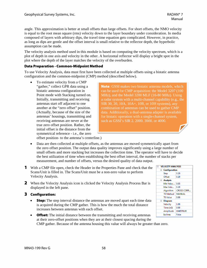
Geophysical Survey Systems, Inc. RADAN® 7 Manual
MN43-199 Rev G 58
angle. This approximation is better at small offsets than large offsets. For short offsets, the NMO velocity is equal to the root mean square (rms) velocity down to the layer boundary under consideration. In media composed of layers with arbitrary dips, the travel time equation gets complicated. However, in practice, as long as dips are gentle and the offset interval is small relative to the reflector depth, the hyperbolic assumption can be made. The velocity analysis method used in this module is based on computing the velocity spectrum, which is a plot of depth in one axis and velocity in the other. A horizontal reflector will display a bright spot in the plot where the depth of the layer matches the velocity of the overburden. Data Preparation - Common-Midpoint Method To use Velocity Analysis, data must first have been collected at multiple offsets using a bistatic antenna configuration and the common-midpoint (CMP) method (described below).
• To estimate velocity from a CMP “gather,” collect GPR data using a bistatic antenna configuration in Point mode with Stacking turned on. Initially, transmitting and receiving antennas start off adjacent to one another at the “zero offset” position. (Actually, because of the size of the antennas’ housings, transmitting and receiving antennas are never at the true zero offset position. Rather, the initial offset is the distance from the symmetrical reference - i.e., the zero offset position- to the antenna’s centerline.)
• Data are then collected at multiple offsets, as the antennas are moved symmetrically apart from the zero offset position. The output data quality improves significantly using a large number of small offsets and more stacking but increases the collection time. The operator will have to decide the best utilization of time when establishing the best offset interval, the number of stacks per measurement, and number of offsets, versus the desired quality of data output.
1 With a CMP file open, check the Header in the Properties Pane and check that the Scans/Unit is filled in. The Scans/Unit must be a non-zero value to perform Velocity Analysis.
2 When the Velocity Analysis icon is clicked the Velocity Analysis Process Bar is displayed in the left pane.
3 Configuration:
• Step: The step interval distance the antennas are moved apart each time data is acquired during the CMP gather. This is how the much the total distance increases between antennas with each offset.
• Offset: The initial distance between the transmitting and receiving antennas at their zero-offset positions when they are at their closest spacing during the CMP gather. Because of the antenna housing this value will always be greater than zero.
Note: GSSI makes two bistatic antenna models, which can be used for CMP acquisition: the Model 3207 (100 MHz), and the Model 3200 MLF (16-80 MHz). Using a radar system with a multi-channel capability (e.g., the SIR 30, 20, 10A, 10A+, 10B, or 10H systems), any combination of antennas can be used to gather CMP data. Additionally, a dual-antenna adapter is available for bistatic operation with a single-channel system, such as GSSI’s SIR 2, 2000, 3000, or 4000.

Geophysical Survey Systems, Inc. RADAN® 7 Manual
MN43-199 Rev G 59
4 Analysis:
• Min Velocity: This is the minimum velocity expected based upon the area where the CMP gather was completed. Adjust this value after running Recalc to improve the display of the velocity in the diagram plot.
• Max Velocity: This is the maximum velocity expected based upon the area where the CMP gather was completed. Adjust this value after running Recalc to improve the display of the velocity in the diagram plot.
• T0 Method: Can choose to derive the Time Zero Position automatically or input it manually.
• T0 Value: Time Zero Position can be entered manually in nS.
5 Once the required information is entered, click the Recalc button and the program will calculate the estimated velocities of the layers present in the data.
6 Diagram:
• Velocity: Show the velocity for a sample as the mouse moves over the diagram.
• Time (nS): Shows the time for a velocity as the mouse moves over the diagram.
• Amplitude: Shows the amplitude for a velocity as the mouse moves over the diagram.
• Line Color: Changes the color of the variable velocity curve as it is drawn on the diagram.
7 Velocity Diagram: When the cursor is placed on the Velocity Diagram, the Velocity, Time (nS), and Amplitude automatically update. • Max: Returns the cursor to the maximum velocity of the
dataset. By clicking Max, the program will automatically pick the maximum velocity layer, place crosshairs at the maximum point, and display the Velocity, Time (nS), and Amplitude.
• Left/Right Arrow: Clicking on the left or right arrow buttons will cause the program to select other layers to display their Velocity, Time (nS), and Amplitude.
• Print: Prints the Velocity Diagram with individual layer information that includes Time (nS), Effective Velocity, Layer Velocity, and Amplitude.
• Save: Saves a .VLC Velocity file. This file can be used during the Migration process instead of doing hyperbola fitting.
• Close: Closes the Velocity Analysis Process Pane. • Recalc: Recalculates the velocity based upon any modified parameters in the
Velocity Analysis Process Pane.
8 Variable Velocity Analysis: Once the parameters under the Velocity Diagram are set the user can create a variable velocity curve based upon the maximum velocity points.

Geophysical Survey Systems, Inc. RADAN® 7 Manual
MN43-199 Rev G 60
• Double-click with the left mouse on the velocity diagram plot. • Position the newly created box over the highest maximum velocity. • Continue to double-click to create additional boxes to match with maximum velocity spots.
9 Velocity Analysis Tab: The Table Pane updates as more velocity points are added in the Velocity Diagram.
10 Click Save to create a .VLC Velocity file that can be used during the Migration process on files collected over the same area as the CMP gather.
Adjust Scans Group
Horizontal Scaling Data may be modified by adjusting the Horizontal Scale using the Stacking, Skipping, and Stretching functions. Stacking can help remove small discreet targets when the user is primarily interested in continuous layers or it can help by averaging out vertical striping in the data caused by the antenna not staying properly coupled with the ground surface. Skipping will compress the data, which may be useful for profiles with long horizontal reflectors. Stretching will expand the data and may improve how horizontal reflectors are visualized. This is particularly helpful if the data were collected in point mode with large step intervals.
1 When the Horizontal Scaling icon is clicked, the left pane will display the Horizontal Scaling Process Bar.
2 Operation: Only one process may be performed at a time. • Stacking: Select Stacking to apply a simple running-average to stack the
data. Stacking combines the adjacent selected radar scans and outputs a single scan. When stacking values are used in RADAN 7, the program will retain the marks in the file. However, the scans per unit distance and marks per unit distance will be changed in the header. For example if there is a raw file with 80 scans per meter and 1 meter per mark and it is stacked by a factor of two (2) the output file would have 40 scans per meter written into the header (reduced by a factor of 2).
• Skipping: Select Skipping to compress the horizontal scale. Specify the number of scans to skip over from the previous scan. For instance, enter 1 to omit every other scan from the file (hence compressing it by a factor of 2).
• Stretching: Select Stretching to expand the horizontal scale. The Stretching function will calculate the simple average of two adjacent scans (or the specified number of scans) and place the averaged scan in between the existing scans.
3 # of Scans: Select number of scans to Stack, Skip, or Stretch.
4 Click Apply to test the process and, if necessary, click Reset and re-adjust.
5 Once satisfied with the process, click OK.
Original Data

Geophysical Survey Systems, Inc. RADAN® 7 Manual
MN43-199 Rev G 61
Stacking (3): Skipping (2): Stretching (2)
Distance Normalization Distance Normalization establishes a constant horizontal scale between marks. This function performs rubber-sheeting so that there is an equal distance, or equal number of scans per unit distance, between markers. This is generally required when data is collected in continuous mode without a survey wheel and is due to unavoidable inconsistencies in antenna towing speed. When Distance Marks or both Distance and User Marks are set Distance Normalization will correct the number of scans between markers by stretching and skipping, thereby correcting for variations in survey speed. Distance Normalization requires that marker information be stored in Way Points tab of the Table Pane. If marker information is not provided the process will generate an error message.
1 Before opening a file that needs Distance Normalization be sure to set the Horizontal and Vertical units (meters, feet, etc.) (Home Ribbon > Units).
2 When the Horizontal Scaling icon is clicked, the left pane will display the Horizontal Scaling Process Bar.
3 Check Markers: Distance Normalization requires a minimum of TWO markers to work. • No double or missing markers. • First and last markers are present. • All User Markers are converted to Distance.
4 The Scans/Unit and the Units/Mark must be assigned a value in the input file header in order for Distance Normalization to work. • Scans/Unit: May be estimated by using the mouse cursor to count the number of scans between
markers or by taking the Scans/Sec value in the header and estimating the number of seconds it took to traverse the distance between marker stations.
• Units/Mark: Determined at the time of the survey. • To use, correctly set the Scans/Unit distance and the Units/Mark in the Header Information
located in the right Properties Pane.

Geophysical Survey Systems, Inc. RADAN® 7 Manual
MN43-199 Rev G 62
5 Apply to User Marks: Set this to Yes to use existing User Marks for Distance Normalization, or No to use the Distance Marks.
6 Click Apply and Reset until achieving the desired results.
7 Click OK to accept the desired reports.
Before Distance Normalization
After Distance Normalization
Note: Distance Normalization is not available for a 3D file.

Geophysical Survey Systems, Inc. RADAN® 7 Manual
MN43-199 Rev G 63
Edit Block Sections of the data can be deleted or saved to create a new file. The original data are not modified as part of this process. It is recommended to change the color palette prior to performing Edit Block in order to see the Picking tool overlay clearly.
1 Change the color palette prior to performing Edit Block in order to see the Picking tool overlay clearly.
2 When the Edit Block icon is selected from the Adjust Scans Group, the left pane will display the Edit Block Process Bar.
3 Click Block Operation and select one of the two options: • Save: Will save the selected area to a new file. • Delete: Will delete the selected area from the original data. A new file
will be generated without the deleted area thereby preserving the original data.
4 Select the Area: There are two ways to choose the area that to delete or save. • Adjust the Picking tool overlay that appears on the linescan to highlight
the part of the data to save or delete. To do this, simply grab the handles of the Picking tool overlay, which will first appear on the left side of the linescan, and drag the mouse to the desired area to save or delete as seen in the image below. While maneuvering the Picking tool overlay on the linescan the Start Scan, End Scan, and Start and End Samples will update accordingly.
• Manually adjust the Start Scan, End Scan, and Start and End Samples in the Edit Block Process Bar.
5 Click OK to process, or Cancel to cancel the operation.

Geophysical Survey Systems, Inc. RADAN® 7 Manual
MN43-199 Rev G 64
Adjust Surface Group
Surface Normalization Surface Normalization assigns an elevation to the markers in the database and corrects for elevation changes. A horizontal or near horizontal reflector may not appear horizontal due to topographic changes. This process corrects for topographic effects. For example, a water table may appear to have significantly greater relief in radar data than in actuality. Surface Normalization corrects for the topography and displays the water table as a flat reflector.
1 When the Surface Normalization icon is selected from the Adjust Surface Group, the left pane will display the Surface Normalization Process Bar. • Normal Level: Shifts the baseline of the data up or down accordingly.
If Auto Level is changed to No the Normal Level can be manually entered. Surface Normalization requires that Distance Marks or both Distance and User Markers be used.
• Vertical Scale: The Vertical Scale may be set to 1:1 (normal view), 1:2, or 1:4. Using the latter two scales compresses the vertical axis (and adjusts the vertical scale accordingly) by factors of 2 and 4, respectively. Compression of the vertical scale may be necessary if the relative change in elevation for the file is greater than the display range of the monitor being used. If data is not compressed, the file may ‘run-off’ the top or the bottom of the display window.
• Auto Level: Automatically sets the level at which the data will be shifted up or down.
2 Click Apply and Reset and make necessary adjustments.
3 Click OK when once desired results are achieved.
Before Surface Normalization
Note: Elevation values have to be manually assigned to the markers using Edit Markers if they are not imported with GPS data. When entered, elevation data will be stored in the Way Points tab of the Table Pane.

Geophysical Survey Systems, Inc. RADAN® 7 Manual
MN43-199 Rev G 65
After Surface Normalization
Static Correction Static Correction compensates for variations in elevation, phase shifts, and high frequency noise present in the horizontal direction and is generally one of the last processing steps undertaken. It compensates for noise introduced from processing, by shifting the reflector within a specified time window (specified by the number of samples) so that it is realigned. Static Correction assumes near-horizontal discontinuous noise due to poor antenna coupling, time zero tracking problems, or some localized changes in the velocity. After a lot of processing, a once horizontal (or near-horizontal) and continuous layer may appear discontinuous and slightly shifted in time, making the reflector difficult to trace from scan to scan. Static Correction can correct for this. Another function of Static Correction is that it filters horizontally without influencing the vertical frequency of the data, unlike with Horizontal High and Low Pass Filtering.
1 Change the color palette prior to performing Static Correction in order to see the Picking tool overlay clearly.
2 When the Static Correction icon is selected from the Adjust Surface Group, the left pane will display the Static Correction Process Bar.
3 Select the horizontal (or near-horizontal) layer for Static Correction.
4 A Picking tool overlay will appear superimposed on the Linescan data. Use the mouse to shape the rectangle to the desired width and move it so it covers the reflector of interest as demonstrated in the image below.

Geophysical Survey Systems, Inc. RADAN® 7 Manual
MN43-199 Rev G 66
5 After adjusting the first segment on the reflector, move the cursor along the reflector clicking with the left mouse button to expand the overlay. In this way, create a multi-segmented window that the Static Correction function will use to trace a reflector.
6 Adjust the window height (in number of samples), the filter length, and the type of model (Boxcar or Triangle) as necessary.
7 Model Base: RADAN 7 creates a model scan of a specified filter length and performs a horizontal boxcar or triangle filter of that specified length using the number of samples in the window and compares it to the highlighted layer. • Type:
o Boxcar Filter: The Boxcar Filter is a rectangular filter window that performs a simple running average on the data. A portion of the data, determined by the filter length, is averaged, and the average is output as a single point at the center of the active portion of the filter window. The filter moves on to the next sample and the process is repeated. The Boxcar filter assigns equal weight to the data all along the filter length.
o Triangular Filter: The Triangular Filter emphasizes the center of the filter more heavily than the ends of the filter. This type of filter is a weighted moving average, with the weighting function shaped like a triangle. A portion of the data, determined by the filter length, is multiplied and summed by this function. The result is output at the center of the triangle. The filter then advances one sample and the process repeats.
• Length: Enter the number of samples to filter.
8 Window Height: Height of search area in samples.
9 Threshold: The correlation threshold is the value used to cross-correlate the model data with the actual data. It is this parameter that determines how well a layer can be traced from scan to scan. The correlation threshold is usually from 0.5 to 1.0.
10 Max Shift: The maximum number of samples a scan can be shifted up or down.
11 Click OK once desired results are achieved.

Geophysical Survey Systems, Inc. RADAN® 7 Manual
MN43-199 Rev G 67
Gain Group Range Gain Range Gain offers a way of changing the gain curve at different points and using different methods. This is helpful if a portion of the data is under or over gained during data collected. There are four Range Gain options available in RADAN 7: Automatic Gain, Linear Gain, Exponential Gain, and Smart (antenna-specific) Gain.
1 When the Range Gain icon is selected from the Gain Group, the left pane will display the Range Gain Process Bar.
2 Select Gain Type:
• Automatic: The Automatic Gain feature attempts to balance the gains over each scan. When the Automatic Gain function is selected, gain corrections are applied to the entire data set. These curves will not only amplify the low amplitude signal but also the high amplitude areas.
• Exponential: The Exponential Gain function applies an exponential gain curve between gain points. Scans are then multiplied by the gain curve.
• Linear: The Linear Gain function applies a linear gain between gain points. Scans are then multiplied by the gain curve.
• Smart: This is an antenna-specific gain curve, which is only available for the SSMini, SSMini HR, Mini EZ, and Mini EZH.
3 Set Channel Parameters if using either Linear or Exponential Gain functions: • # of Points: Number of sections the data is equally divided vertically. • Overall Gain (dB): For the Automatic Gain the overall gain factor is normally set between 2 and
5. Only applicable to Automatic Gain. • Horiz TC (scans): A value for the horizontal time constant is required to run the Automatic Gain
function. This time constant determines how many scans on the left side of the current scan will be used to shape the automatic gain curve. It applies a weighted filter. A small value giving more weight to scans adjacent to the current scan, a large value giving weight to those further away. The horizontal time constant is normally set between 11 and 21. Only applicable to Automatic Gain.
4 Adjust Gain Points: Linear Gains and Exponential Gains are applied manually and allow the user to manipulate the amount of gain between gain points by either changing the gain in the value box or by dragging the gain points (small squares) on the Oscope to the right or left. It is recommended to set the number of gain points between 4 and 8, but RADAN 7 allows for 16 gain points.
5 Clipping: While adjusting the gain points it is important that the wiggle trace stay within the view of the Oscope window. If the wiggle trace extends beyond the limits of this window clipping will occur and portions of the data beyond the screen will be removed. This will over gain the data.
6 Click Apply and Reset, and make any necessary adjustments.
7 Click OK desired results are achieved.

Geophysical Survey Systems, Inc. RADAN® 7 Manual
MN43-199 Rev G 68
Before Range Gain After Range Gain
Gain Restoration The Gain Restoration function removes the gain applied to the data during acquisition. Restoring gain is an important option if the data are to be exported to a forward modeling program, or determine the dielectric permittivity, conductivity, and dispersion (approximate attenuation) of layers. The Gain Restoration function uses gain information found in the file header to remove the gain function and normalize the gains.
1 When the Gain Restoration icon is selected from the Gain Group, the left pane will display the Gain Restoration Process Bar.
2 Channel Parameters:
• Overall Gain: Enter the display gain value to apply to the data after the gain applied during data collection is removed.
• Sample: Enter Starting and Ending Samples to apply Gain Restoration.
3 Click Apply and Reset, and adjust if necessary.
4 Click OK once desired results are achieved.
Note: Gain differences exceeding 30 dB may result in a significant loss in data resolution. Saturated data will result in distorted wavelets after Gain Restoration.
After Gain Restoration

Geophysical Survey Systems, Inc. RADAN® 7 Manual
MN43-199 Rev G 69
Waveform Group
Hilbert XForm A Hilbert Transform is used to display subtle properties of the earth. Reflector amplitude and time are the primary types of information in GPR data used to make interpretations. Another way of defining the data is by transforming it into frequency and phase (positive or negative changes in the scan trace). This information is sometimes more sensitive to important subsurface (dielectric) changes in the amplitude or geometric information. A Hilbert Transform will change a radar signal represented as a time series into its magnitude (via envelope detection), instantaneous phase, or instantaneous frequency components (the derivative of phase). The Hilbert Transform expresses the relationship between the phase and magnitude of the signal, or between its real and imaginary parts. It allows the phase of a signal to be reconstructed from its amplitude.
1 When the Hilbert Transform icon is selected from the Waveform Group, the left pane will display the Hilbert Transform Process Bar.
2 Channel Parameters:
• Transform:
o Magnitude: The magnitude display is useful for indicating the raw energy reflected from an object or layer.
o Phase: The radar wavelet itself may not always be a clear indicator of energy levels because it consists of several cycles.
o Frequency: The instantaneous frequency indicates how the earth is filtering the radar signal. This sets the maximum frequency that will be output.
• Samples: Enter Starting and Ending Samples to apply the Hilbert Transformation.
3 Click Apply and Reset, and adjust if necessary.
4 Click OK once desired results are achieved.
Before Hilbert XForm After Hilbert XForm

Geophysical Survey Systems, Inc. RADAN® 7 Manual
MN43-199 Rev G 70
Deconvolution Multiples or “ringing” occur when the radar signal bounces back and forth between an object (such as a piece of metal or layer of wet clay) and the antenna, causing repetitive reflection patterns throughout the data and obscuring information at lower depths. Multiple reflections may also be observed when mapping water bottom, bedrock (or till), or voids. Deconvolution is the filtering method used to remove this type of noise or interference. RADAN 7 uses a method called Predictive Deconvolution, which is aptly named because it tries to approximate the shape of the transmitted pulse as the antenna is coupled to the ground. This method tries to approximate the shape of the transmitted pulse as the antenna is coupled to the ground. Assuming a source wavelet of a specified length, called the operator length, this filter will predict what the data will look like a certain distance away, called the prediction lag, when the source wavelet is subtracted (or deconvolved) from it. This results in the compression of the reflected wavelet. Predictable phenomena, such as antenna ringing and multiples, are moved to distances greater than the prediction lag and are effectively removed from the data.
1 When the Deconvolution icon is selected from the Waveform Group, the left pane will display the Deconvolution Process Bar.
2 Channel Parameters: In order for Deconvolution to work properly, certain parameters, such as operator length, prediction lag, prewhitening, gain, start sample, and end sample, must be supplied as inputs. • Operator Length: The operator length specifies the size of the filter
used in terms of the number of samples making up 1 pulse length. Longer filters give a better approximation of the radar wavelet and generally give better results. A good rule to start with is that the operator length should be about one full cycle of the radar antenna wavelet. A value less than this gives poor results. o Measure: Measure the width of a reverb in number of samples. o Enter: Set the operator length to that value. Increase the operator length slightly for more
effect. • Prediction Lag: The Prediction Lag should be set to the desired length of the output pulses
(about one-half cycle of the antenna wavelet). Anything smaller than this will produce more noise. When using Deconvolution to remove multiple reflections, the lag should be equal to or less than the spacing between multiples. A prediction lag between 5 and 1 is used to approximate “spiking” deconvolution, which matches and removes the wavelet. However, this introduces significantly more noise into the data.
• Prewhitening: Prewhitening modifies the autocorrelation function by boosting the white noise (zero delay) component. Mathematically, prewhitening stabilizes the filter, thereby smoothing the output and reducing noise. Values between 1 and 10 percent are common, 8 percent is a good value to start with.
• Overall Gain: Overall Gain may be needed because the deconvolution process attenuates the signal, especially when the prediction lag is short. Gain values of 3 to 5 are common, but use whatever achieves an amplitude level equal to the original data.
• Samples: The starting and ending sample should be set to establish the “time gate," specified in terms of sample number, in which the Deconvolution filter is active. For instance, a start sample

Geophysical Survey Systems, Inc. RADAN® 7 Manual
MN43-199 Rev G 71
and end sample of 256 and 1024 respectively may be used to remove multiples beneath a reflector located at sample number 240 in a 1024 Samples/Scan data set.
3 Click Apply and Reset, and adjust if necessary.
4 Click OK once desired results are achieved.
Before Deconvolution After Deconvolution
Other Group
Math Simple arithmetic functions may be performed on the data by using the Math processing option. In includes steps to subtract another file, add or multiply by another constant, or express data in terms of its absolute value, square root, or integrate the data.
1 When the Math icon is selected from the Other Group, the left pane will display the Math Process Bar.
2 Channel Parameters:
• Before Function: It is possible to add, subtract, and multiply by a constant before performing a nonlinear function. o Add Constant: Add or Subtract values to or from the sample. o Multiply Constant: Multiple the sample by a given value.
• Function: The Arithmetic Function provides options to perform a number of linear and nonlinear functions. When designing an operation, be aware that the original data is only 8 bits, it will range from -128 to 127 before the math operation. After the operation, the output file will still be 8 bits, any overflows as a result of the operation will be clipped.

Geophysical Survey Systems, Inc. RADAN® 7 Manual
MN43-199 Rev G 72
o Negate: y(t) = - x(t): Reverses the phase of the scan trace thereby making positive peaks negative and negative peaks positive.
o Absolute Value (ABS): y(t) = | x(t) |: Takes the absolute value of each peak.
o Differentiate: y(t) = x(t) - x(t-1):
o Integrate: y(t) = x(t) + x(t-1) + x(t-2) +… :
o Square: y(t) = (x(t)) 2: Using the Exponential or Squared function, this can emphasize strong (high amplitude) signals and reduce or remove weak (low amplitude) signals or noise.
o Square Root (SQRT): y(t) = (x(t)) 1/2: When using Log or Square Root functions, data amplitudes must be expressed as positive numbers (i.e., data cannot be zero or negative). Otherwise, an error will occur resulting from an improper mathematical procedure. Therefore, first take the absolute value of the data. This function emphasizes low amplitude data relative to high amplitude data.
o Log: y(t) = ln [x(t)], where ln[x(t)] is the natural logarithm: When using Log or Square Root functions, data amplitudes must be expressed as positive numbers (i.e., data cannot be zero or negative). Otherwise, an error will occur resulting from an improper mathematical procedure. Therefore, first take the absolute value of the data. This function emphasizes low amplitude data relative to high amplitude data.
o Exponent (Exp): y(t) = Exp [x(t)] or e[x(t)]: Using the Exponential or Squared function can emphasize strong (high amplitude) signals and reduce or remove weak (low amplitude) signals or noise.
• After Function: It is possible to add and multiply by a constant after performing a nonlinear function. o Multiply 2nd Constant: Add or Subtract values to or from the sample. o Add 2nd Constant: Multiple the sample by a given value.
• Samples: Enter Starting and Ending Samples to apply the Math function.
3 Click Apply and Reset, and adjust if necessary.
4 Click OK once desired results are achieved.
Note: When using some functions such as Log or Square Root, data amplitudes must be expressed as positive numbers (i.e., data cannot be zero or negative). Otherwise, an error will occur resulting from an improper mathematical procedure. Therefore, first take the absolute value of the data. Therefore, the Log, Exponent, Square, or Square Root functions may need to be combined with constant multiplication and addition in order to obtain output within the proper range. This is why multiplication and addition are allowed before (1st add constant and 1st multiply constant, respectively) and after (2nd add constant and 2nd multiply constant, respectively) the function.

Geophysical Survey Systems, Inc. RADAN® 7 Manual
MN43-199 Rev G 73
Peaks Extraction The Peaks Extraction function will automatically trace continuous reflections in the data window of the active file according to the user specified selection parameters. It is used to emphasize strong reflections.
1 When the Peaks Extraction icon is selected from the Other Group, the left pane will display the Peaks Extraction Process Bar.
2 Select: Defines if the function will trace all peaks, only the positive peaks, or only the negative peaks.
3 Max # of Points: Defines the number of peaks to trace. The indicated number of strong reflections will be displayed. Reflections may vary along the profile, but their total number in any trace will not exceed the Max #.
4 Samples/Point: Defines the width of the peaks in the vertical directions. The peaks are displayed as bands of the indicated width, with the amplitude values preserved within these bands. The rest of the data is set to zero.
5 Start and End Samples: By default the entire trace is processed, but the user may choose any horizontal layer, expressed in sample numbers. Only the selected interval will be processed, the rest of the file is left unchanged.
6 Click Apply and Reset, and adjust if necessary.
7 Click OK once desired results are achieved.
Before Peaks Extraction.

Geophysical Survey Systems, Inc. RADAN® 7 Manual
MN43-199 Rev G 74
Following Peaks Extraction.
Cross Channel Math The Cross Channel Math function creates combinations of channels and assigns them to a selected channel in a multi-channel file. A selection of arithmetic operations is available for this operation.
1 When the Cross Channel Math icon is selected from the Other Group, the left pane will display the Cross Channel Math Process Bar.
2 Select Channel: When multiple channels are available choose which one to apply the Cross Channel Math function to. For a single-channel file, Cross Channel Math means an arithmetic function will be performed on that channel.
3 Channel Parameters:
• Function:
o NONE: No transformation. o ADD: Adds the channel. o SUB: Subtracts the channel. o ADD3: Add 3 numbers. o SQADD: Square root of the absolute value of the sum of the channels. o SQSUB: Square root of the absolute value of the difference of the
channels. o SQDIV: Square root of the absolute value of the division of the
channels. o SQMUL: Square root of the absolute value of the product of the
channels. o VSUMM: Square root of the sum of the squares of the two channels. o VSUMM3: Square root of the sum of the squares of the three channels.

Geophysical Survey Systems, Inc. RADAN® 7 Manual
MN43-199 Rev G 75
• Gain Compensation: Removes applied gain from each component before function. • Comp 1: Channel number mapped to the component. • Gain 1: Gain applied to the component. • Comp 2-3: Channel number of other component used in Functions other than NONE. • Gain 2-3: Gain applied to the corresponding component.
4 Click Apply and Reset, and adjust if necessary.
5 Click OK once desired results are achieved.
Channel Blending The Channel Blending function serves to blend two separate channels of data into one profile. It is intended to combine high and low frequency data, such as that collected with the UtilityScan DF.
1 When the Channel Blending icon is selected from the Other Group, the left pane will display the Channel Blending Process Bar.
2 Percent Position: Where on Channel 1 the blending will begin.
3 Percent Width: Width of the blending centered on the position where the blending will occur.
4 Click Apply and Reset, and adjust if necessary.
5 Click OK once desired results are achieved.
Note: The output from Channel Blending is placed in Channel 2 and replaces the original Channel 2 data. The first channel of data is still available in Channel 1.
Prior to Channel Blending.

Geophysical Survey Systems, Inc. RADAN® 7 Manual
MN43-199 Rev G 76
Following Channel Blending.
Auto Target – Automated Process If data were collected using GSSI’s Structure Scan Mini, this option will automatically pick targets by placing Dots on the apex’s of the hyperbolic reflections. Each of the Dots will appear as in the Targets Tab as a separate target. The Target Picks tab will have all of the depth and velocity information for each of the Dots.
Signal Floor – Automated Process This function analyzes the noise and signal loss (attenuation) from scan to scan and provides estimate of the effective depth penetration. Real reflectors may still be located beneath the Signal Floor if they are strong enough. The output of this function is shown as a green line on the screen, as seen below, and saved as a .BII binary file.
1 When the Signal Floor icon is clicked, the left pane will display the Max Depth Process Bar.
2 Signal Floor Estimator: If multiple channels of data were collected, choose between which channels to use to estimate max depth.
3 Simply click Apply and Reset to test this processing function. Click OK to accept the setting and generate the binary file.

Geophysical Survey Systems, Inc. RADAN® 7 Manual
MN43-199 Rev G 77
2D Interactive This ribbon allows you to add targets and layers to your 2D data and display them in 3D.
Interactive Status Group
Show Toggles On or Off the targets and layers already added to the data. Selecting Show does not enable the rest of the 2D Interactive Ribbon. That requires selecting Add or Edit.
Add or Edit When selected the targets or layers already added to the data will be displayed and you can either edit the existing interpretations or add new ones. Selecting Add or Edit enables the rest of the 2D Interactive Ribbon.
Objects Group
Pick Type There are two types of objects that can be added to the data; Targets or Layers. Pick between Target or Layer to choose which gets added or modified.
Focus This specifies which Target or Layer is being added or modified. If multiple Targets have already been drawn they will appear in the drop down menu. The drop down menu is also used to select a new Layer.
New Target Click here to draw additional targets. This option is only available when adding Targets and does apply to adding more layers. Those are added by using Focus.
Pick Attributes Group
Pick Polarity When picking targets or layers, the user may specify which portion of the reflection to attach new picks to Positive, Negative, Absolute, or None polarity.
Search Width In pixels, enter the search width for the Single Point picking tool.
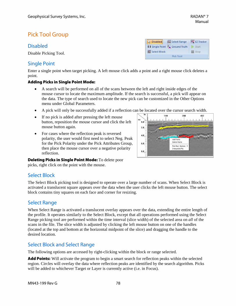
Geophysical Survey Systems, Inc. RADAN® 7 Manual
MN43-199 Rev G 78
Pick Tool Group
Disabled Disable Picking Tool.
Single Point Enter a single point when target picking. A left mouse click adds a point and a right mouse click deletes a point. Adding Picks in Single Point Mode:
• A search will be performed on all of the scans between the left and right inside edges of the mouse cursor to locate the maximum amplitude. If the search is successful, a pick will appear on the data. The type of search used to locate the new pick can be customized in the Other Options menu under Global Parameters.
• A pick will only be successfully added if a reflection can be located over the cursor search width. • If no pick is added after pressing the left mouse
button, reposition the mouse cursor and click the left mouse button again.
• For cases where the reflection peak is reversed polarity, the user would first need to select Neg. Peak for the Pick Polarity under the Pick Attributes Group, then place the mouse cursor over a negative polarity reflection.
Deleting Picks in Single Point Mode: To delete poor picks, right click on the point with the mouse.
Select Block The Select Block picking tool is designed to operate over a large number of scans. When Select Block is activated a translucent square appears over the data when the user clicks the left mouse button. The select block contains tiny squares on each face and corner for resizing.
Select Range When Select Range is activated a translucent overlay appears over the data, extending the entire length of the profile. It operates similarly to the Select Block, except that all operations performed using the Select Range picking tool are performed within the time interval (slice width) of the selected area on all of the scans in the file. The slice width is adjusted by clicking the left mouse button on one of the handles (located at the top and bottom at the horizontal midpoint of the slice) and dragging the handle to the desired location.
Select Block and Select Range The following options are accessed by right-clicking within the block or range selected. Add Points: Will activate the program to begin a smart search for reflection peaks within the selected region. Circles will overlay the data where reflection peaks are identified by the search algorithm. Picks will be added to whichever Target or Layer is currently active (i.e. in Focus).

Geophysical Survey Systems, Inc. RADAN® 7 Manual
MN43-199 Rev G 79
Delete Points: Will activate the program to start deleting the picks of the current Target or Layer located within the selected region. Pick Modification Options
• Change Pick ID: Change the layer or target number assigned to the picks located within the selected region. For example, the user desires to change the layer # of a group of Layer 3 picks to Layer 2. The user must select layer 3 as the Current Layer, position the Select Block (or Select Range) over the group of points and click the right mouse button to access the Pick Modification Options. Select Change Pick ID to switch from Layer 3 to Layer 2.
• Change Pick Velocity: Changes the velocity of the currently selected layer picks located in the selected region. It opens a dialog box for entering the desired velocity. The user can choose to either specify the new velocity, use the nearest core, or ground truth, data, or use results from velocity analysis. Choosing Lock Velocity keeps the data from being change with subsequent velocity modifications.
Interpolate Points: Will interpolate layer picks (add new picks between existing ones) using the interpolation method (Linear or Nearest Neighbor) specified in Global Parameters under Interpolation Method.
Ground Truth Selecting the Ground Truth icon allows the user to individually adjust the depth of picks based upon a true measured depth. As depths are entered they appear in the Target or Layer Ground Truth tab of the Table Pane. To enter individual Ground Truth information:
• Select Ground Truth from the Interactive Mode window. • Click in the data the spot where the ground truth was collected. • Enter the depth. • Click OK or Cancel.
To specify all new layer picks to have velocities calculated from the ground truth data, change the Vel. Method from Default Vel. to Core Data in the Layer tab of the Table.
EZ Tracker Allows the user to add a layer or targets by interpolating data between mouse clicks.
1 Choose Pick Type and choose the appropriate layer or target to Focus (edit).
2 Start: Select to start EZ Tracker. Add layer picks with the left mouse button and delete layer picks with the right mouse button. Picks are interpolated between left mouse button clicks. The closer the click spacing the better the results will be.
3 Right-click to undo the previous selection. This only goes back one time.
Note: A selected point is not changed to the new layer if a pick from the new layer is already present in the scan, or if the new layer overlaps another layer pick (i.e., changing a Layer 3 pick to a Layer 1 pick with a Layer 2 pick present in the scan).

Geophysical Survey Systems, Inc. RADAN® 7 Manual
MN43-199 Rev G 80
4 Stop: Select to stop EZ Tracker.
5 If there are breaks in the layer then select and Stop and Start to skip the break.
Other Options Group
Global Parameters Single Pt. Search Length: When using Single Point Picking Tool, this setting determines whether the pick is entered at the closest peak or using the cursor length. Amplitude Values: Use Data Units, decibels (dB), or Normalized dB.
• Data Units: Provides the layer bottom reflection amplitudes in the actual data values.
• dB: Converts the data units amplitudes to decibels (dB) by using the equation 20*log10(x) where x is the absolute value of the data amplitude.
• Normalized dB: Normalizes the data amplitude relative to 32767 for 16 bit data and 2147483648 for 32 bit data before converting to dB.
Interpolation Method: Each time a pick is added a search is performed to locate the corresponding feature of the reflection that will be used to identify two-way travel time and amplitude. Use either Automatic, Nearest Peak, or Linear.
• Automatic: Performs tracking based on a custom algorithm, which is designed to capture continuous layers that vary with depth. When mouse clicks are spaced more than 20 scans apart this mode switches to Nearest Peak.
• Nearest Peak: Search for the nearest peak between existing picks. • Linear: Draws a straight line between two previously interpreted picks.
Checking the box will fill the layer with a chosen color in depth pane. Click OK or Cancel. Help will open a .pdf of the RADAN 7 manual.
Non-Filled Layers Filled Layers

Geophysical Survey Systems, Inc. RADAN® 7 Manual
MN43-199 Rev G 81
Settings Load Default Settings: Loads previously saved default settings for Interactive Mode. Save As Default Settings: Saves the current Interactive Mode settings including all layer properties and display options.
Display Gain To change the Display Gain, click Display Gain in the Home Ribbon or right-click on the data window and select Display Gain. Then select from a preset list of multiples ranging from -6 up to 60. Input a Custom Value by right-clicking and selecting Custom from Display Gain menu. This will change all samples, no matter where they are in the scan trace, by the same amount.
• Altering the display gain does not change data values like Range Gain, which is described later in this section under the Easy Processing and Processing sections.
• Altering the display gain may make it easier to see lower amplitude targets.
Export Group Picks may be exported to a comma delimited ASCII (CSV) file, saved as a JPG image file, or the layer information exported to a KML file (if GPS was collected with the data) for viewing in Google Earth.
CSV File Click CSV File to export picks to a comma delimited ASCII file and select which fields to export. Use Existing: Use existing custom fields that were created in Create Custom or are available for specific applications from GSSI.
• Select an Available Export Configuration. • Modify Options for Filtering Data as necessary. • Save the exported CSV file.
Create Custom: Select fields to export. • Select the desired Export Category. • Choose which Available Fields to include in the CSV
file. • Choose whether to export all of the data or specify
ranges or certain values. If filtering exported data, then modify Options for Filtering Data as necessary.
• Name the custom export. Create a general name for use with other data. • Save the exported CSV File.
Modify Existing: Modify an existing field list to create a new one. • Select an Available Export Configuration. • Select the desired Export Category. • Choose which Available Fields to include in the CSV file.
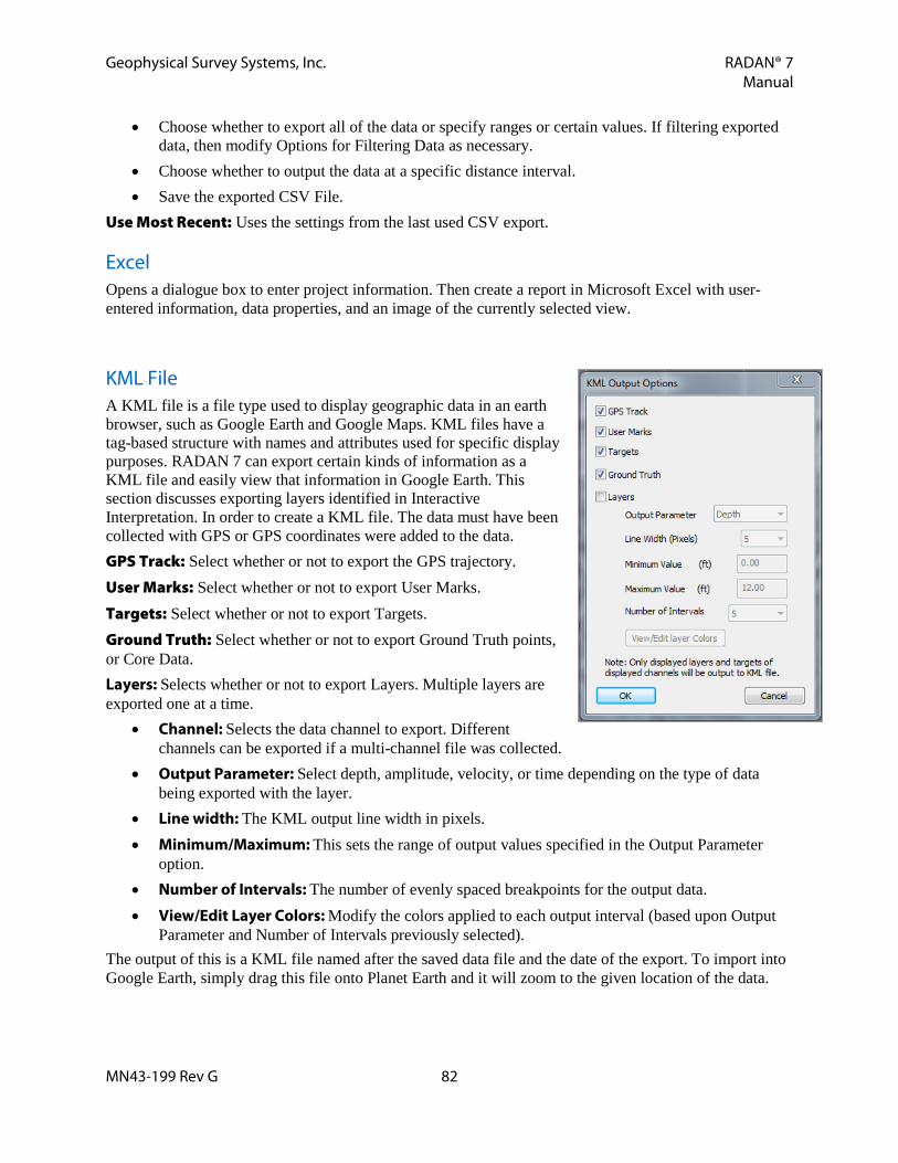
Geophysical Survey Systems, Inc. RADAN® 7 Manual
MN43-199 Rev G 82
• Choose whether to export all of the data or specify ranges or certain values. If filtering exported data, then modify Options for Filtering Data as necessary.
• Choose whether to output the data at a specific distance interval. • Save the exported CSV File.
Use Most Recent: Uses the settings from the last used CSV export.
Excel Opens a dialogue box to enter project information. Then create a report in Microsoft Excel with user-entered information, data properties, and an image of the currently selected view.
KML File A KML file is a file type used to display geographic data in an earth browser, such as Google Earth and Google Maps. KML files have a tag-based structure with names and attributes used for specific display purposes. RADAN 7 can export certain kinds of information as a KML file and easily view that information in Google Earth. This section discusses exporting layers identified in Interactive Interpretation. In order to create a KML file. The data must have been collected with GPS or GPS coordinates were added to the data.
GPS Track: Select whether or not to export the GPS trajectory. User Marks: Select whether or not to export User Marks. Targets: Select whether or not to export Targets. Ground Truth: Select whether or not to export Ground Truth points, or Core Data. Layers: Selects whether or not to export Layers. Multiple layers are exported one at a time.
• Channel: Selects the data channel to export. Different channels can be exported if a multi-channel file was collected.
• Output Parameter: Select depth, amplitude, velocity, or time depending on the type of data being exported with the layer.
• Line width: The KML output line width in pixels. • Minimum/Maximum: This sets the range of output values specified in the Output Parameter
option. • Number of Intervals: The number of evenly spaced breakpoints for the output data. • View/Edit Layer Colors: Modify the colors applied to each output interval (based upon Output
Parameter and Number of Intervals previously selected). The output of this is a KML file named after the saved data file and the date of the export. To import into Google Earth, simply drag this file onto Planet Earth and it will zoom to the given location of the data.

Geophysical Survey Systems, Inc. RADAN® 7 Manual
MN43-199 Rev G 83
StructureScan Ribbon The StructureScan Ribbon offers quick processing and viewing of 3D structure scan data. Individual 3D grids can also be combined to create larger combined grid files.
Processing Since concrete is typically a homogenous composition processing can be automated. The Processing Group incorporates standard processing methods for structure scan data.
1 When the Structure icon is selected from the Processing Group, the left pane will display the Structure Process Bar.
2 Custom Options: Select which options for automatic processing by toggling between Yes and No. • Auto Time-Zero: Auto locate and adjust time-zero. • Smart Background Removal: This filter removes
horizontal bands of noise. • Auto-Amplitude Correction: Performs an automatic
amplitude adjustment.
3 Click Apply and Reset, and adjust if necessary.
4 Click OK once desired results are achieved.
StructureScan data prior to running the Structure function.
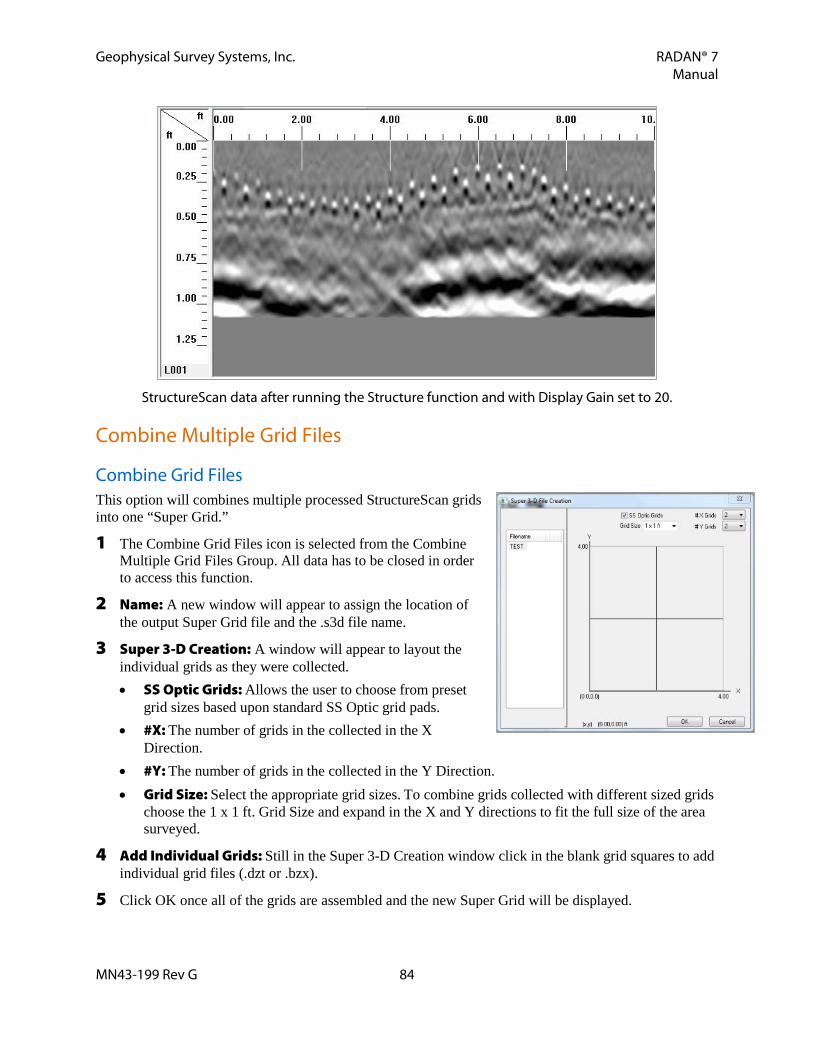
Geophysical Survey Systems, Inc. RADAN® 7 Manual
MN43-199 Rev G 84
StructureScan data after running the Structure function and with Display Gain set to 20.
Combine Multiple Grid Files
Combine Grid Files This option will combines multiple processed StructureScan grids into one “Super Grid.”
1 The Combine Grid Files icon is selected from the Combine Multiple Grid Files Group. All data has to be closed in order to access this function.
2 Name: A new window will appear to assign the location of the output Super Grid file and the .s3d file name.
3 Super 3-D Creation: A window will appear to layout the individual grids as they were collected. • SS Optic Grids: Allows the user to choose from preset
grid sizes based upon standard SS Optic grid pads. • #X: The number of grids in the collected in the X
Direction. • #Y: The number of grids in the collected in the Y Direction. • Grid Size: Select the appropriate grid sizes. To combine grids collected with different sized grids
choose the 1 x 1 ft. Grid Size and expand in the X and Y directions to fit the full size of the area surveyed.
4 Add Individual Grids: Still in the Super 3-D Creation window click in the blank grid squares to add individual grid files (.dzt or .bzx).
5 Click OK once all of the grids are assembled and the new Super Grid will be displayed.

Geophysical Survey Systems, Inc. RADAN® 7 Manual
MN43-199 Rev G 85
Depth Slice Viewing View Depth Slices Display a top-down view of data and slice through difference depths.
Z-Slice Z-Slice Depth: Adjust the depth of the slice for viewing.
Depth Slice Control Full Thickness Slice: Check this to see full view from top to bottom, uncheck to be able to view data in slices and change Slice Thickness. Thickness: Adjust the thickness of the slice. Maximum Depth: Adjust the maximum depth of the data.
Note: The color and color transform can be modified under the Home Ribbon. There are also multiple ways to view different depth slices.
• Use Depth Slice Control. • Use the 3D Slice Controls
Window under the View Ribbon. • Press the CTRL key while holding
the left mouse button and move the mouse up and down.

Geophysical Survey Systems, Inc. RADAN® 7 Manual
MN43-199 Rev G 86
RoadScan Ribbon The RoadScan Ribbon provides viewing and processing options for data collected specifically for determining pavement layer thickness.
Window Group The Window Group includes five different ways view either the data or the data properties.
Scope This will display an O-Scope to the right of the linescan data. Hold the left mouse button down while pointing to the linescan data to correspond with the O-Scope using a horizontal line.
Location Used primarily for 3D Grid files or individual profiles with GPS data, this will display a grid showing the location of each profile.
• By holding the left mouse button down on the linescan data the location of that spot on the grid can be determined.
• Right-clicking inside of the grid with the mouse will either Move 3D Area, which can change the starting coordinates of the grid, or access the GPS Coordinates menu to add or modify the GPS Coordinates for the grid.
• Right-clicking on the ends of lines with the mouse will either Nudge Profile, which shifts the profile forward or backward along the line, or Edit Profile Coordinates, which can change the profiles location within the grid.
Depth Pane Toggles the Interactive Interpretation Pane On or Off below the linescan display.
Processing Group The Processing Group includes steps for horn calibration, reflection picking, and layer interpretation.
Horn Calibration Settings from the horn calibration are stored with the processed data file header and accessed when the calibration file is used in the reflection picking tool.
1 When the Horn Calibration icon is selected from the Processing Group, the left pane will display the Horn Calibration Process Bar.
2 Automatic Mode: “Yes” is the recommended method and performs an automatic horn calibration or choose to select custom calibration settings.

Geophysical Survey Systems, Inc. RADAN® 7 Manual
MN43-199 Rev G 87
3 Use Air Wave File: The airwave file is most commonly collected by turning the antennas upside down so that they radiate upward. This file is obtained using the same SIR 10/20/30 settings as the metal plate calibration file. Use of an air wave file is optional and not typically used. • No: No air wave file was collected or one is not being used. • Yes: An air wave file has been collected. Enter the air wave filename in the space to the right.
4 # of Channels: Number of channels in the data file currently open.
5 Channel: Choose which channel to calibrate. Setting this to ALL will process all of the channels with common parameters. • Antenna Type: Select the antenna used for data collection. • Serial Number: Serial number of chosen
antenna if it is a Smart antenna.
6 Click Apply and Reset, and adjust if necessary.
7 Click OK once desired results are achieved. It is recommended that the .CZT calibration file is saved with an easily recognizable name to identify it during processing.
Reflection Picking Reflection Picking corrects the ground surface of RoadScan data based on the previously created Horn Calibration .CZT file. This process eliminates unwanted signal noise to enhance reflections from the pavement layers making them easier to track. Measures the return times of the reflections and calculates the two-way travel time for each of the pavement layers from the data.
1 When the Reflection Picking icon is selected from the Processing Group, the left pane will display the Reflection Picking Process Bar.
2 Cal(ibration) File Select Method: Select the method for identifying the .CZT, calibration file. • User Select: Manually choose the calibration file. • Current Output Folder: Will search for a .CZT file in the current Output Directory specified in
Global Parameters under the Properties Pane prior to opening any data. • Antenna Database: If there is a serial number and model number an antenna database will
automatically be created. If survey conditions are consistent enough the user does have to recollect a calibration file prior to each survey. Instead the antenna database can be used.
• Auto Select: If Auto Save is set to No it will search the current Output Directory specified in Global Parameters. If the Auto Save is set to Yes it will look in the Proc folder that is automatically created within the Source Directory as specified in Global Parameters. If more than one .CZT is located in the specified folder, RADAN 7 will select the first one in alphanumeric order. If no .CZT file is found it will search the antenna database.
3 Automatic Mode: Select whether or not to use standard settings. If No is selected the following options are available. • Background Removal: Removes horizontal banding in the data. • Starting Depth: Specifies the starting depth for Background Removal.
Note: RADAN 7 will automatically save the Horn Calibration file to the Proc folder if Auto Save is set to Yes in the Global Parameters.

Geophysical Survey Systems, Inc. RADAN® 7 Manual
MN43-199 Rev G 88
• Apply Inline Position Correction: Correct for inline offset specified in Channel Positions tab of the Table Pane.
4 Click Apply and Reset, and adjust if necessary.
5 Click OK once desired settings are achieved. RADAN 7 will prompt the user to specify an antenna calibration file.
Layer Interpretation The Layer Interpretation option is designed to automatically track layers in road structures that exhibit clear and consistent layer reflections. The output is identical to the manually derived output of EZ Tracker, but under certain controlled conditions Layer Interpretation can make layer picking automated. This process works best for layers that with high amplitude reflections that are continuous, but even under ideal conditions, the output from Layer Interpretation will still require manual editing using Single Point, Select Block, or Select Range. Layer Interpretation can only be performed on files that have been generated from the Reflection Picking process.
1 When the Layer Interpretation icon is selected from the Processing Group, the left pane will display the Layer Interpretation Process Bar.
2 Automatic Mode: Works for clearly visible single layers. • Number of Layers: Enter the number of layers that RADAN 7 is trying to identify. This value
will typically be 1 as it works best with a single layer. • Minimum Depth: Enter the minimum depth of the first layer. This allows the user to set the
search range deeper than the ground surface reflection. Otherwise the ground surface reflection may be picked as a layer unintentionally.
3 Click Apply and Reset, and adjust if necessary.
4 Click OK once desired results are achieved.
Interactive Status Group
Show Toggles On or Off the targets and layers already added to the data. Selecting Show does not enable the rest of the 2D Interactive Ribbon. That requires selecting Add or Edit.
Add or Edit When selected the targets or layers already added to the data will be displayed and you can either edit the existing interpretations or add new ones. Selecting Add or Edit enables the rest of the 2D Interactive Ribbon.
Note: For steps on how to manually edit the Layer Interpretation output refer to the Interactive Group section.

Geophysical Survey Systems, Inc. RADAN® 7 Manual
MN43-199 Rev G 89
2D Interactive Group After processing Road data, click on Add or Edit from the Interactive Status Group to begin picking and editing targets. This enables options for inserting and deleting targets or layers identified in the data. Targets can be exported as an ASCII comma delimited file for use in other software.
Pick Type There are two types of objects that can be added to the data; Targets or Layers. Pick between Target or Layer to choose which gets added or modified.
Focus This specifies which Target or Layer is being added or modified. If multiple Targets have already been drawn they will appear in the drop down menu. The drop down menu is also used to select a new Layer.
New Target Click here to draw additional targets. This option is only available when adding Targets and does apply to adding more layers. Those are added by using Focus.
Pick Polarity When picking targets or layers, the user may specify which portion of the reflection to attach new picks to Positive, Negative, Absolute, or None polarity.
Search Width In pixels, enter the search width for the Single Point picking tool.
Disabled Disable Picking Tool.
Single Point Enter a single point when target picking. A left mouse click adds a point and a right mouse click deletes a point. Adding Picks in Single Point Mode:
• A search will be performed on all of the scans between the left and right inside edges of the mouse cursor to locate the maximum amplitude. If the search is successful, a pick will appear on the data. The type of search used to locate the new pick can be customized in the Other Options menu under Global Parameters.
• A pick will only be successfully added if a reflection can be located over the cursor search width. • If no pick is added after pressing the left mouse button, reposition the mouse cursor and click the
left mouse button again.

Geophysical Survey Systems, Inc. RADAN® 7 Manual
MN43-199 Rev G 90
• For cases where the reflection peak is reversed polarity, the user would first need to select Neg. Peak for the Pick Polarity under the Pick Attributes Group, then place the mouse cursor over a negative polarity reflection.
Deleting Picks in Single Point Mode: To delete poor picks, right click on the point with the mouse.
Select Block The Select Block picking tool is designed to operate over a large number of scans. When Select Block is activated a translucent square appears over the data when the user clicks the left mouse button. The select block contains tiny squares on each face and corner for resizing.
Select Range When Select Range is activated a translucent overlay appears over the data, extending the entire length of the profile. It operates similarly to the Select Block, except that all operations performed using the Select Range picking tool are performed within the time interval (slice width) of the selected area on all of the scans in the file. The slice width is adjusted by clicking the left mouse button on one of the handles (located at the top and bottom at the horizontal midpoint of the slice) and dragging the handle to the desired location.
Select Block and Select Range The following options are accessed by right-clicking within the block or range selected. Add Points: Will activate the program to begin a smart search for reflection peaks within the selected region. Circles will overlay the data where reflection peaks are identified by the search algorithm. Picks will be added to whichever Target or Layer is currently active (i.e. in Focus). Delete Points: Will activate the program to start deleting the picks of the current Target or Layer located within the selected region. Pick Modification Options
• Change Pick ID: Change the layer or target number assigned to the picks located within the selected region. For example, the user desires to change the layer # of a group of Layer 3 picks to Layer 2. The user must select layer 3 as the Current Layer, position the Select Block (or Select Range) over the group of points and click the right mouse button to access the Pick Modification Options. Select Change Pick ID to switch from Layer 3 to Layer 2.
• Change Pick Velocity: Changes the velocity of the currently selected layer picks located in the selected region. It opens a dialog box for entering the desired velocity. The user can choose to either specify the new velocity, use the nearest core, or ground truth, data, or use results from velocity analysis. Choosing Lock Velocity keeps the data from being change with subsequent velocity modifications.
Note: A selected point is not changed to the new layer if a pick from the new layer is already present in the scan, or if the new layer overlaps another layer pick (i.e., changing a Layer 3 pick to a Layer 1 pick with a Layer 2 pick present in the scan).
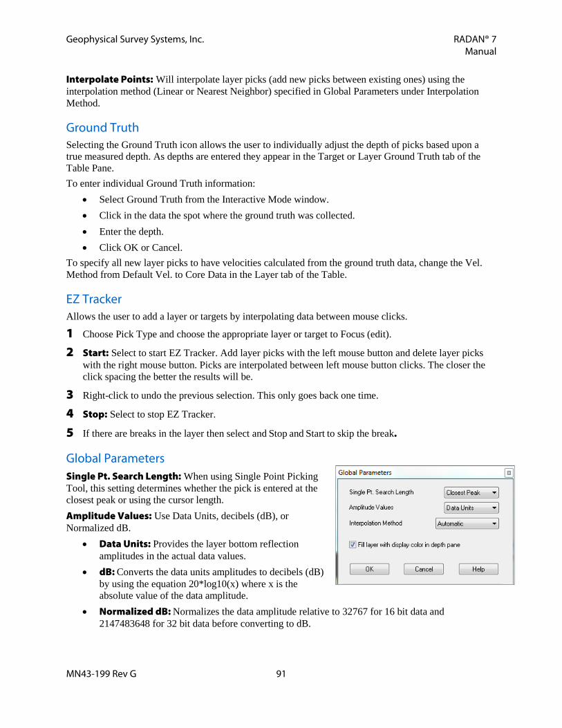
Geophysical Survey Systems, Inc. RADAN® 7 Manual
MN43-199 Rev G 91
Interpolate Points: Will interpolate layer picks (add new picks between existing ones) using the interpolation method (Linear or Nearest Neighbor) specified in Global Parameters under Interpolation Method.
Ground Truth Selecting the Ground Truth icon allows the user to individually adjust the depth of picks based upon a true measured depth. As depths are entered they appear in the Target or Layer Ground Truth tab of the Table Pane. To enter individual Ground Truth information:
• Select Ground Truth from the Interactive Mode window. • Click in the data the spot where the ground truth was collected. • Enter the depth. • Click OK or Cancel.
To specify all new layer picks to have velocities calculated from the ground truth data, change the Vel. Method from Default Vel. to Core Data in the Layer tab of the Table.
EZ Tracker Allows the user to add a layer or targets by interpolating data between mouse clicks.
1 Choose Pick Type and choose the appropriate layer or target to Focus (edit).
2 Start: Select to start EZ Tracker. Add layer picks with the left mouse button and delete layer picks with the right mouse button. Picks are interpolated between left mouse button clicks. The closer the click spacing the better the results will be.
3 Right-click to undo the previous selection. This only goes back one time.
4 Stop: Select to stop EZ Tracker.
5 If there are breaks in the layer then select and Stop and Start to skip the break.
Global Parameters Single Pt. Search Length: When using Single Point Picking Tool, this setting determines whether the pick is entered at the closest peak or using the cursor length. Amplitude Values: Use Data Units, decibels (dB), or Normalized dB.
• Data Units: Provides the layer bottom reflection amplitudes in the actual data values.
• dB: Converts the data units amplitudes to decibels (dB) by using the equation 20*log10(x) where x is the absolute value of the data amplitude.
• Normalized dB: Normalizes the data amplitude relative to 32767 for 16 bit data and 2147483648 for 32 bit data before converting to dB.
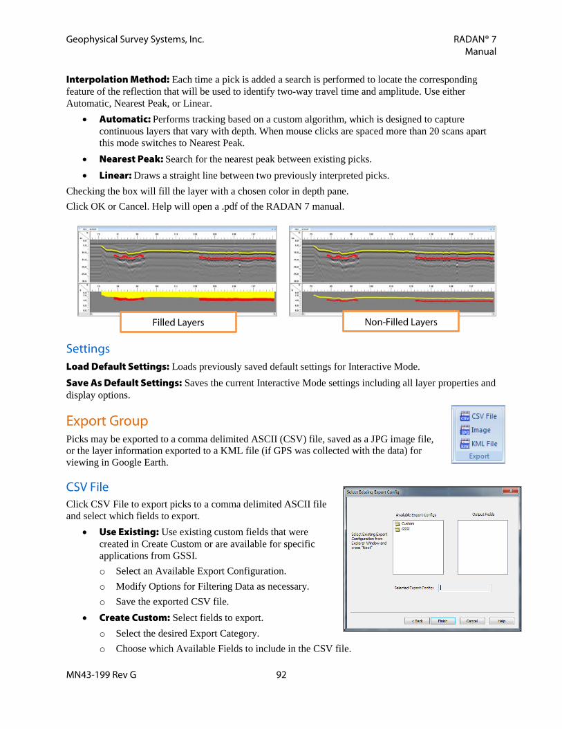
Geophysical Survey Systems, Inc. RADAN® 7 Manual
MN43-199 Rev G 92
Interpolation Method: Each time a pick is added a search is performed to locate the corresponding feature of the reflection that will be used to identify two-way travel time and amplitude. Use either Automatic, Nearest Peak, or Linear.
• Automatic: Performs tracking based on a custom algorithm, which is designed to capture continuous layers that vary with depth. When mouse clicks are spaced more than 20 scans apart this mode switches to Nearest Peak.
• Nearest Peak: Search for the nearest peak between existing picks. • Linear: Draws a straight line between two previously interpreted picks.
Checking the box will fill the layer with a chosen color in depth pane. Click OK or Cancel. Help will open a .pdf of the RADAN 7 manual.
Settings Load Default Settings: Loads previously saved default settings for Interactive Mode. Save As Default Settings: Saves the current Interactive Mode settings including all layer properties and display options.
Export Group Picks may be exported to a comma delimited ASCII (CSV) file, saved as a JPG image file, or the layer information exported to a KML file (if GPS was collected with the data) for viewing in Google Earth.
CSV File Click CSV File to export picks to a comma delimited ASCII file and select which fields to export.
• Use Existing: Use existing custom fields that were created in Create Custom or are available for specific applications from GSSI. o Select an Available Export Configuration. o Modify Options for Filtering Data as necessary. o Save the exported CSV file.
• Create Custom: Select fields to export. o Select the desired Export Category. o Choose which Available Fields to include in the CSV file.
Non-Filled Layers Filled Layers
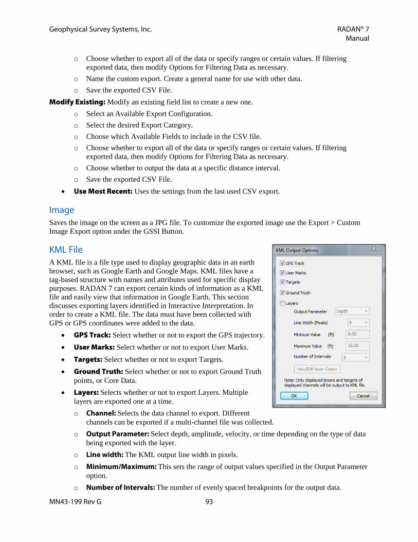
Geophysical Survey Systems, Inc. RADAN® 7 Manual
MN43-199 Rev G 93
o Choose whether to export all of the data or specify ranges or certain values. If filtering exported data, then modify Options for Filtering Data as necessary.
o Name the custom export. Create a general name for use with other data. o Save the exported CSV File.
Modify Existing: Modify an existing field list to create a new one. o Select an Available Export Configuration. o Select the desired Export Category. o Choose which Available Fields to include in the CSV file. o Choose whether to export all of the data or specify ranges or certain values. If filtering
exported data, then modify Options for Filtering Data as necessary. o Choose whether to output the data at a specific distance interval. o Save the exported CSV File.
• Use Most Recent: Uses the settings from the last used CSV export.
Image Saves the image on the screen as a JPG file. To customize the exported image use the Export > Custom Image Export option under the GSSI Button.
KML File A KML file is a file type used to display geographic data in an earth browser, such as Google Earth and Google Maps. KML files have a tag-based structure with names and attributes used for specific display purposes. RADAN 7 can export certain kinds of information as a KML file and easily view that information in Google Earth. This section discusses exporting layers identified in Interactive Interpretation. In order to create a KML file. The data must have been collected with GPS or GPS coordinates were added to the data.
• GPS Track: Select whether or not to export the GPS trajectory. • User Marks: Select whether or not to export User Marks. • Targets: Select whether or not to export Targets. • Ground Truth: Select whether or not to export Ground Truth
points, or Core Data. • Layers: Selects whether or not to export Layers. Multiple
layers are exported one at a time. o Channel: Selects the data channel to export. Different
channels can be exported if a multi-channel file was collected. o Output Parameter: Select depth, amplitude, velocity, or time depending on the type of data
being exported with the layer. o Line width: The KML output line width in pixels. o Minimum/Maximum: This sets the range of output values specified in the Output Parameter
option. o Number of Intervals: The number of evenly spaced breakpoints for the output data.

Geophysical Survey Systems, Inc. RADAN® 7 Manual
MN43-199 Rev G 94
o View/Edit Layer Colors: Modify the colors applied to each output interval (based upon Output Parameter and Number of Intervals previously selected).
The output of this is a KML file named after the saved data file and the date of the export. To import into Google Earth, simply drag this file onto Planet Earth and it will zoom to the given location of the data.

Geophysical Survey Systems, Inc. RADAN® 7 Manual
MN43-199 Rev G 95
BridgeScan Ribbon The BridgeScan Ribbon is designed to process data specifically collected to determine bridge deterioration.
Window Group The Window Group includes five different ways view either the data or the data properties.
Scope This will display an O-Scope to the right of the linescan data. Hold the left mouse button down while pointing to the linescan data to correspond with the O-Scope using a horizontal line.
Location Used primarily for 3D Grid files or individual profiles with GPS data, this will display a grid showing the location of each profile.
• By holding the left mouse button down on the linescan data the location of that spot on the grid can be determined.
• Right-clicking inside of the grid with the mouse will either Move 3D Area, which can change the starting coordinates of the grid, or access the GPS Coordinates menu to add or modify the GPS Coordinates for the grid.
• Right-clicking on the ends of lines with the mouse will either Nudge Profile, which shifts the profile forward or backward along the line, or Edit Profile Coordinates, which can change the profiles location within the grid.
Depth Pane Toggles the Interactive Interpretation Pane On or Off below the linescan display.
Create 3D File A step-by-step guide combining collected files, processing the files, and preparing the newly created “bridge” file for further processing. Creation of a 3D file is necessary to complete Bridge Deterioration Mapping, but is not necessary for Bridge QA.
1 Click Create 3D File.
2 Browse to the appropriate folder where the collected bridge files are located.
3 Create an output filename for the newly created bridge 3D file.
4 Click Next.

Geophysical Survey Systems, Inc. RADAN® 7 Manual
MN43-199 Rev G 96
5 Add the bridge files from the left pane to the right pane by: • Double-clicking on the File, or • Click on the File and click Add > , or • If Appropriate, click Add All, or • Highlight a group of files and click Add > • Remove files from the right pane by doing the same
procedures in the right pane
6 Click Next.
7 File Group 3D Area: • Enter the length of the bridge. • Enter the starting distance of the FIRST line collected from the Curb or Lane Stripe. • Enter the spacing between each profile or line. • Click the down arrow to select how the data were
collected. • Select whether the data were collected Standard or
Inline.
8 Click Next.
9 Adjust File Group Details: Can edit the individual profiles. • Filename: The name of each file collected. • Across Dist.: The distance from the curb of each of the
files collected. • Rev. Dir.: If the files were collected in a zig-zag
pattern and this was specified, an X will automatically be entered that the file will need to be reversed.
• St. Loc.: This is the starting location of the file • Edit St. Loc.: Correct the starting location of the file as
necessary. • End Loc.: This is the ending location of the file. • Edit End Loc.: Correct the ending location of the file
as necessary.
10 Edit the Starting and Ending Locations of each file follow these steps. • Click Edit St. Loc. or Edit End Loc. for EACH file,
one at a time. • Move the slider bar until the vertical line on the data matches the beginning of the bridge. This
point will likely correspond with the middle of the bridge joint. Use the left and right arrow keys on the keyboard to make minor adjustments, as well as clicking on the up and down arrows on the screen
• Click OK.

Geophysical Survey Systems, Inc. RADAN® 7 Manual
MN43-199 Rev G 97
• Repeat this process for the Starting and Ending Locations for ALL files.
11 Click Next.
12 Enter the Bridge Joint Skew Angle: This will be a positive number if the bridge is angled to the right and negative number if the bridge is angled to the left.
13 Click Finish.
Processing Group
Bridge QA This section describes data collection for quality assurance (QA) studies on concrete overlaid bridge decks. This technique is not applicable to asphalt overlaid decks. The goal of this application is to ensure that there is adequate concrete cover over the top layer of reinforcing steel. A single representative profile per travel lane is all that is required to perform Bridge QA. Typically, this profile is along the wheel path of the lane as opposed to the shoulder. The data must be collected perpendicular to the trend of the top layer of rebar. This means that if the rebar are longitudinal, the profiles must be collected across the bridge deck, not along it. If a complete map of cover thickness is required, then a 3D file can be collected following the instructions given in the SIR System manual. Be sure to configure the data collection settings (Gain, Position, Range, Scan and Sample density).
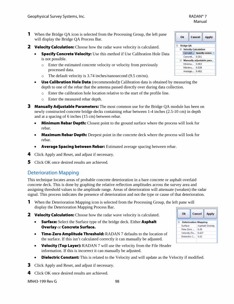
Geophysical Survey Systems, Inc. RADAN® 7 Manual
MN43-199 Rev G 98
1 When the Bridge QA icon is selected from the Processing Group, the left pane will display the Bridge QA Process Bar.
2 Velocity Calculation: Choose how the radar wave velocity is calculated. • Specify Concrete Velocity: Use this method if Use Calibration Hole Data
is not possible. o Enter the estimated concrete velocity or velocity from previously
processed data. o The default velocity is 3.74 inches/nanosecond (9.5 cm/ns).
• Use Calibration Hole Data (recommended): Calibration data is obtained by measuring the depth to one of the rebar that the antenna passed directly over during data collection. o Enter the calibration hole location relative to the start of the profile line. o Enter the measured rebar depth.
3 Manually Adjustable Parameters: The most common use for the Bridge QA module has been on newly constructed concrete bridge decks containing rebar between 1-4 inches (2.5-10 cm) in depth and at a spacing of 6 inches (15 cm) between rebar. • Minimum Rebar Depth: Closest point to the ground surface where the process will look for
rebar. • Maximum Rebar Depth: Deepest point in the concrete deck where the process will look for
rebar. • Average Spacing between Rebar: Estimated average spacing between rebar.
4 Click Apply and Reset, and adjust if necessary.
5 Click OK once desired results are achieved.
Deterioration Mapping This technique locates areas of probable concrete deterioration in a bare concrete or asphalt overlaid concrete deck. This is done by graphing the relative reflection amplitudes across the survey area and assigning threshold values to the amplitude range. Areas of deterioration will attenuate (weaken) the radar signal. This process indicates the presence of deterioration and not the type or cause of that deterioration.
1 When the Deterioration Mapping icon is selected from the Processing Group, the left pane will display the Deterioration Mapping Process Bar.
2 Velocity Calculation: Choose how the radar wave velocity is calculated. • Surface: Select the Surface type of the bridge deck. Either Asphalt
Overlay or Concrete Surface. • Time-Zero Amplitude Threshold: RADAN 7 defaults to the location of
the surface. If this isn’t calculated correctly it can manually be adjusted. • Velocity (Top Layer): RADAN 7 will use the velocity from the File Header
information. If this is incorrect it can manually be adjusted. • Dielectric Constant: This is related to the Velocity and will update as the Velocity if modified.
3 Click Apply and Reset, and adjust if necessary.
4 Click OK once desired results are achieved.

Geophysical Survey Systems, Inc. RADAN® 7 Manual
MN43-199 Rev G 99
Interactive Status Group
Show Toggles On or Off the targets and layers already added to the data. Selecting Show does not enable the rest of the 2D Interactive Ribbon. That requires selecting Add or Edit.
Add or Edit When selected the targets or layers already added to the data will be displayed and you can either edit the existing interpretations or add new ones. Selecting Add or Edit enables the rest of the 2D Interactive Ribbon.
2D Interactive Group After processing Bridge data, click on Add or Edit from the Interactive Status Group to begin picking and editing targets. This enables options for inserting and deleting targets or layers identified in the data. Targets can be exported as an ASCII comma delimited file for use in other software.
Pick Type There are two types of objects that can be added to the data; Targets or Layers. Pick between Target or Layer to choose which gets added or modified.
Focus This specifies which Target or Layer is being added or modified. If multiple Targets have already been drawn they will appear in the drop down menu. The drop down menu is also used to select a new Layer.
New Target Click here to draw additional targets. This option is only available when adding Targets and does apply to adding more layers. Those are added by using Focus.
Pick Polarity When picking targets or layers, the user may specify which portion of the reflection to attach new picks to Positive, Negative, Absolute, or None polarity.
Search Width In pixels, enter the search width for the Single Point picking tool.
Disabled Disable Picking Tool.

Geophysical Survey Systems, Inc. RADAN® 7 Manual
MN43-199 Rev G 100
Single Point Enter a single point when target picking. A left mouse click adds a point and a right mouse click deletes a point. Adding Picks in Single Point Mode:
• A search will be performed on all of the scans between the left and right inside edges of the mouse cursor to locate the maximum amplitude. If the search is successful, a pick will appear on the data. The type of search used to locate the new pick can be customized in the Other Options menu under Global Parameters.
• A pick will only be successfully added if a reflection can be located over the cursor search width. • If no pick is added after pressing the left mouse button, reposition the mouse cursor and click the
left mouse button again. • For cases where the reflection peak is reversed polarity, the user would first need to select Neg.
Peak for the Pick Polarity under the Pick Attributes Group, then place the mouse cursor over a negative polarity reflection.
Deleting Picks in Single Point Mode: To delete poor picks, right click on the point with the mouse.
Select Block The Select Block picking tool is designed to operate over a large number of scans. When Select Block is activated a translucent square appears over the data when the user clicks the left mouse button. The select block contains tiny squares on each face and corner for resizing.
Select Range When Select Range is activated a translucent overlay appears over the data, extending the entire length of the profile. It operates similarly to the Select Block, except that all operations performed using the Select Range picking tool are performed within the time interval (slice width) of the selected area on all of the scans in the file. The slice width is adjusted by clicking the left mouse button on one of the handles (located at the top and bottom at the horizontal midpoint of the slice) and dragging the handle to the desired location.
Select Block and Select Range The following options are accessed by right-clicking within the block or range selected. Add Points: Will activate the program to begin a smart search for reflection peaks within the selected region. Circles will overlay the data where reflection peaks are identified by the search algorithm. Picks will be added to whichever Target or Layer is currently active (i.e. in Focus). Delete Points: Will activate the program to start deleting the picks of the current Target or Layer located within the selected region.

Geophysical Survey Systems, Inc. RADAN® 7 Manual
MN43-199 Rev G 101
Pick Modification Options • Change Pick ID: Change the layer or target number assigned to the picks located within the
selected region. For example, the user desires to change the layer # of a group of Layer 3 picks to Layer 2. The user must select layer 3 as the Current Layer, position the Select Block (or Select Range) over the group of points and click the right mouse button to access the Pick Modification Options. Select Change Pick ID to switch from Layer 3 to Layer 2.
• Change Pick Velocity: Changes the velocity of the currently selected layer picks located in the selected region. It opens a dialog box for entering the desired velocity. The user can choose to either specify the new velocity, use the nearest core, or ground truth, data, or use results from velocity analysis. Choosing Lock Velocity keeps the data from being change with subsequent velocity modifications.
Interpolate Points: Will interpolate layer picks (add new picks between existing ones) using the interpolation method (Linear or Nearest Neighbor) specified in Global Parameters under Interpolation Method.
Ground Truth Selecting the Ground Truth icon allows the user to individually adjust the depth of picks based upon a true measured depth. As depths are entered they appear in the Target or Layer Ground Truth tab of the Table Pane. To enter individual Ground Truth information:
• Select Ground Truth from the Interactive Mode window. • Click in the data the spot where the ground truth was collected. • Enter the depth. • Click OK or Cancel.
To specify all new layer picks to have velocities calculated from the ground truth data, change the Vel. Method from Default Vel. to Core Data in the Layer tab of the Table.
EZ Tracker Allows the user to add a layer or targets by interpolating data between mouse clicks.
1 Choose Pick Type and choose the appropriate layer or target to Focus (edit).
2 Start: Select to start EZ Tracker. Add layer picks with the left mouse button and delete layer picks with the right mouse button. Picks are interpolated between left mouse button clicks. The closer the click spacing the better the results will be.
3 Right-click to undo the previous selection. This only goes back one time.
Note: A selected point is not changed to the new layer if a pick from the new layer is already present in the scan, or if the new layer overlaps another layer pick (i.e., changing a Layer 3 pick to a Layer 1 pick with a Layer 2 pick present in the scan).

Geophysical Survey Systems, Inc. RADAN® 7 Manual
MN43-199 Rev G 102
4 Stop: Select to stop EZ Tracker.
5 If there are breaks in the layer then select and Stop and Start to skip the break.
Global Parameters Single Pt. Search Length: When using Single Point Picking Tool, this setting determines whether the pick is entered at the closest peak or using the cursor length. Amplitude Values: Use Data Units, decibels (dB), or Normalized dB.
• Data Units: Provides the layer bottom reflection amplitudes in the actual data values.
• dB: Converts the data units amplitudes to decibels (dB) by using the equation 20*log10(x) where x is the absolute value of the data amplitude.
• Normalized dB: Normalizes the data amplitude relative to 32767 for 16 bit data and 2147483648 for 32 bit data before converting to dB.
Interpolation Method: Each time a pick is added a search is performed to locate the corresponding feature of the reflection that will be used to identify two-way travel time and amplitude. Use either Automatic, Nearest Peak, or Linear.
• Automatic: Performs tracking based on a custom algorithm, which is designed to capture continuous layers that vary with depth. When mouse clicks are spaced more than 20 scans apart this mode switches to Nearest Peak.
• Nearest Peak: Search for the nearest peak between existing picks. • Linear: Draws a straight line between two previously interpreted picks.
Checking the box will fill the layer with a chosen color in depth pane. Click OK or Cancel. Help will open a .pdf of the RADAN 7 manual.
Settings Load Default Settings: Loads previously saved default settings for Interactive Mode. Save As Default Settings: Saves the current Interactive Mode settings including all layer properties and display options.
Non-Filled Layers Filled Layers

Geophysical Survey Systems, Inc. RADAN® 7 Manual
MN43-199 Rev G 103
Export Group Picks may be exported to a comma delimited ASCII (CSV) file, saved as a JPG image file, or the layer information exported to a KML file (if GPS was collected with the data) for viewing in Google Earth.
CSV File Click CSV File to export picks to a comma delimited ASCII file and select which fields to export.
• Use Existing: Use existing custom fields that were created in Create Custom or are available for specific applications from GSSI. o Select an Available Export Configuration. o Modify Options for Filtering Data as necessary. o Save the exported CSV file.
• Create Custom: Select fields to export. o Select the desired Export Category. o Choose which Available Fields to include in the CSV
file. o Choose whether to export all of the data or specify
ranges or certain values. If filtering exported data, then modify Options for Filtering Data as necessary.
o Name the custom export. Create a general name for use with other data.
o Save the exported CSV File. • Modify Existing: Modify an existing field list to create a
new one. o Select an Available Export Configuration. o Select the desired Export Category. o Choose which Available Fields to include in the CSV file. o Choose whether to export all of the data or specify ranges or certain values. If filtering
exported data, then modify Options for Filtering Data as necessary. o Choose whether to output the data at a specific distance interval. o Save the exported CSV File.
• Use Most Recent: Uses the settings from the last used CSV export.
Image Saves the image on the screen as a JPG file. To customize the exported image use the Export > Custom Image Export option under the GSSI Button.

Geophysical Survey Systems, Inc. RADAN® 7 Manual
MN43-199 Rev G 104
KML File A KML file is a file type used to display geographic data in an earth browser, such as Google Earth and Google Maps. KML files have a tag-based structure with names and attributes used for specific display purposes. RADAN 7 can export certain kinds of information as a KML file and easily view that information in Google Earth. This section discusses exporting layers identified in Interactive Interpretation. In order to create a KML file. The data must have been collected with GPS or GPS coordinates were added to the data.
• GPS Track: Select whether or not to export the GPS trajectory. • User Marks: Select whether or not to export User Marks. • Targets: Select whether or not to export Targets. • Ground Truth: Select whether or not to export Ground Truth
points, or Core Data. • Layers: Selects whether or not to export Layers. Multiple layers
are exported one at a time. o Channel: Selects the data channel to export. Different
channels can be exported if a multi-channel file was collected. o Output Parameter: Select depth, amplitude, velocity, or time depending on the type of data
being exported with the layer. o Line width: The KML output line width in pixels. o Minimum/Maximum: This sets the range of output values specified in the Output Parameter
option. o Number of Intervals: The number of evenly spaced breakpoints for the output data. o View/Edit Layer Colors: Modify the colors applied to each output interval (based upon
Output Parameter and Number of Intervals previously selected). The output of this is a KML file named after the saved data file and the date of the export. To import into Google Earth, simply drag this file onto Planet Earth and it will zoom to the given location of the data.

Geophysical Survey Systems, Inc. RADAN® 7 Manual
MN43-199 Rev G 105
Horn BridgeScan Ribbon The Horn BridgeScan Ribbon is designed to process data specifically collected to determine bridge deterioration using an air-launched horn antenna instead of a ground-coupled antenna.
Window Group The Window Group includes five different ways view either the data or the data properties.
Scope This will display an O-Scope to the right of the linescan data. Hold the left mouse button down while pointing to the linescan data to correspond with the O-Scope using a horizontal line.
Location Used primarily for 3D Grid files or individual profiles with GPS data, this will display a grid showing the location of each profile.
• By holding the left mouse button down on the linescan data the location of that spot on the grid can be determined.
• Right-clicking inside of the grid with the mouse will either Move 3D Area, which can change the starting coordinates of the grid, or access the GPS Coordinates menu to add or modify the GPS Coordinates for the grid.
• Right-clicking on the ends of lines with the mouse will either Nudge Profile, which shifts the profile forward or backward along the line, or Edit Profile Coordinates, which can change the profiles location within the grid.
Depth Pane Toggles the Interactive Interpretation Pane On or Off below the linescan display.
Calibration Horn Calibration: Settings from the horn calibration are stored with the processed data file header and accessed when the calibration file is used in the reflection picking tool.
1 When the Horn Calibration icon is selected from the Processing Group, the left pane will display the Horn Calibration Process Bar.
2 Automatic Mode: “Yes” is the recommended method and performs an automatic horn calibration or choose to select custom calibration settings.
3 Use Air Wave File: The airwave file is most commonly collected by turning the antennas upside down so that they radiate upward. This file is obtained using the same SIR 10/20/30 settings as the metal plate calibration file. Use of an air wave file is optional and not typically used. • No: No air wave file was collected or one is not being used. • Yes: An air wave file has been collected. Enter the air wave filename in the space to the right.

Geophysical Survey Systems, Inc. RADAN® 7 Manual
MN43-199 Rev G 106
4 # of Channels: Number of channels in the data file currently open.
5 Channel: Choose which channel to calibrate. Setting this to ALL will process all of the channels with common parameters. • Antenna Type: Select the antenna used for data collection. • Serial Number: Serial number of chosen antenna if it is a Smart antenna.
6 Click Apply and Reset, and adjust if necessary.
7 Click OK once desired results are achieved. It is recommended that the .CZT calibration file is saved with an easily recognizable name to identify it during processing.
Create 3D File A step-by-step guide combining collected files, processing the files, and preparing the newly created “bridge” file for further processing. Creation of a 3D file is necessary to complete Bridge Deterioration Mapping, but is not necessary for Bridge QA.
1 Click Create 3D File.
2 Browse to the appropriate folder where the collected bridge files are located.
3 Create an output filename for the newly created bridge 3D file.
4 Click Next.
5 Add the bridge files from the left pane to the right pane by: • Double-clicking on the File, or • Click on the File and click Add > , or • If Appropriate, click Add All, or • Highlight a group of files and click Add > • Remove files from the right pane by doing the
same procedures in the right pane
6 Click Next.
Note: RADAN 7 will automatically save the Horn Calibration file to the Proc folder if Auto Save is set to Yes in the Global Parameters.
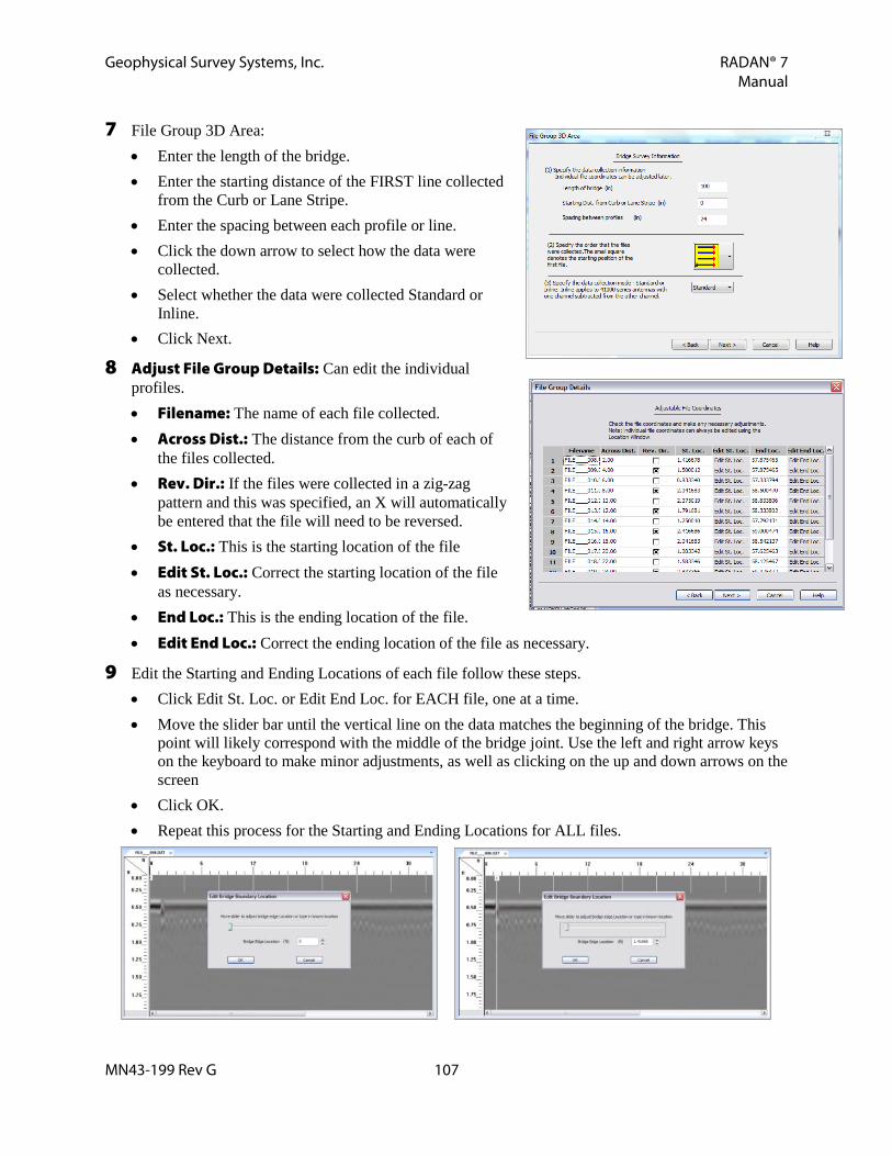
Geophysical Survey Systems, Inc. RADAN® 7 Manual
MN43-199 Rev G 107
7 File Group 3D Area: • Enter the length of the bridge. • Enter the starting distance of the FIRST line collected
from the Curb or Lane Stripe. • Enter the spacing between each profile or line. • Click the down arrow to select how the data were
collected. • Select whether the data were collected Standard or
Inline. • Click Next.
8 Adjust File Group Details: Can edit the individual profiles. • Filename: The name of each file collected. • Across Dist.: The distance from the curb of each of
the files collected. • Rev. Dir.: If the files were collected in a zig-zag
pattern and this was specified, an X will automatically be entered that the file will need to be reversed.
• St. Loc.: This is the starting location of the file • Edit St. Loc.: Correct the starting location of the file
as necessary. • End Loc.: This is the ending location of the file. • Edit End Loc.: Correct the ending location of the file as necessary.
9 Edit the Starting and Ending Locations of each file follow these steps. • Click Edit St. Loc. or Edit End Loc. for EACH file, one at a time. • Move the slider bar until the vertical line on the data matches the beginning of the bridge. This
point will likely correspond with the middle of the bridge joint. Use the left and right arrow keys on the keyboard to make minor adjustments, as well as clicking on the up and down arrows on the screen
• Click OK. • Repeat this process for the Starting and Ending Locations for ALL files.

Geophysical Survey Systems, Inc. RADAN® 7 Manual
MN43-199 Rev G 108
10 Click Next.
11 Enter the Bridge Joint Skew Angle: This will be a positive number if the bridge is angled to the right and negative number if the bridge is angled to the left.
12 Click Finish.
Processing Group Reflection Picking Reflection Picking corrects the ground surface of RoadScan data based on the previously created Horn Calibration .CZT file. This process eliminates unwanted signal noise to enhance reflections from the pavement layers making them easier to track. Measures the return times of the reflections and calculates the two-way travel time for each of the pavement layers from the data.
1 When the Reflection Picking icon is selected from the Processing Group, the left pane will display the Reflection Picking Process Bar.
2 Cal(ibration) File Select Method: Select the method for identifying the .CZT, calibration file. • User Select: Manually choose the calibration file. • Current Output Folder: Will search for a .CZT file in the current Output Directory specified in
Global Parameters under the Properties Pane prior to opening any data. • Antenna Database: If there is a serial number and model number an antenna database will
automatically be created. If survey conditions are consistent enough the user does have to recollect a calibration file prior to each survey. Instead the antenna database can be used.
• Auto Select: If Auto Save is set to No it will search the current Output Directory specified in Global Parameters. If the Auto Save is set to Yes it will look in the Proc folder that is automatically created within the Source Directory as specified in Global Parameters. If more than one .CZT is located in the specified folder, RADAN 7 will select the first one in alphanumeric order. If no .CZT file is found it will search the antenna database.
3 Automatic Mode: Select whether or not to use standard settings. If No is selected the following options are available. • Background Removal: Removes horizontal banding in the data. • Starting Depth: Specifies the starting depth for Background Removal. • Apply Inline Position Correction: Correct for inline offset specified in Channel Positions tab
of the Table Pane.
4 Click Apply and Reset, and adjust if necessary.
5 Click OK once desired settings are achieved. RADAN 7 will prompt the user to specify an antenna calibration file.

Geophysical Survey Systems, Inc. RADAN® 7 Manual
MN43-199 Rev G 109
Horn Bridge Analysis This technique locates areas of probable concrete deterioration in a bare concrete or asphalt overlaid concrete deck. This is done by graphing the relative reflection amplitudes across the survey area and assigning threshold values to the amplitude range. Areas of deterioration will attenuate (weaken) the radar signal. This process indicates the presence of deterioration and not the type or cause of that deterioration.
1 When the Deterioration Mapping icon is selected from the Processing Group, the left pane will display the Deterioration Mapping Process Bar.
2 Velocity Calculation: Choose how the radar wave velocity is calculated. • Surface: Select the Surface type of the bridge deck. Either Asphalt Overlay
or Concrete Surface. • Time-Zero Amplitude Threshold: RADAN 7 defaults to the location of the
surface. If this isn’t calculated correctly it can manually be adjusted. • Velocity (Top Layer): RADAN 7 will use the velocity from the File
Header information. If this is incorrect it can manually be adjusted. • Dielectric Constant: This is related to the Velocity and will update as the Velocity if modified.
3 Click Apply and Reset, and adjust if necessary.
4 Click OK once desired results are achieved.
Preset Lists Group Asphalt and Concrete: Links directly to the Proc. Lists Tab in the Data, Processes, & Proc. Lists Pane. Choosing either Asphalt or Concrete will automatically run a set group of processes (macros). This allows the user to quickly apply more commonly used settings for data collected over roads a Concrete Surface or those with an Asphalt Overlay.
Interactive Status Group
Show Toggles On or Off the targets and layers already added to the data. Selecting Show does not enable the rest of the 2D Interactive Ribbon. That requires selecting Add or Edit.
Add or Edit When selected the targets or layers already added to the data will be displayed and you can either edit the existing interpretations or add new ones. Selecting Add or Edit enables the rest of the 2D Interactive Ribbon.
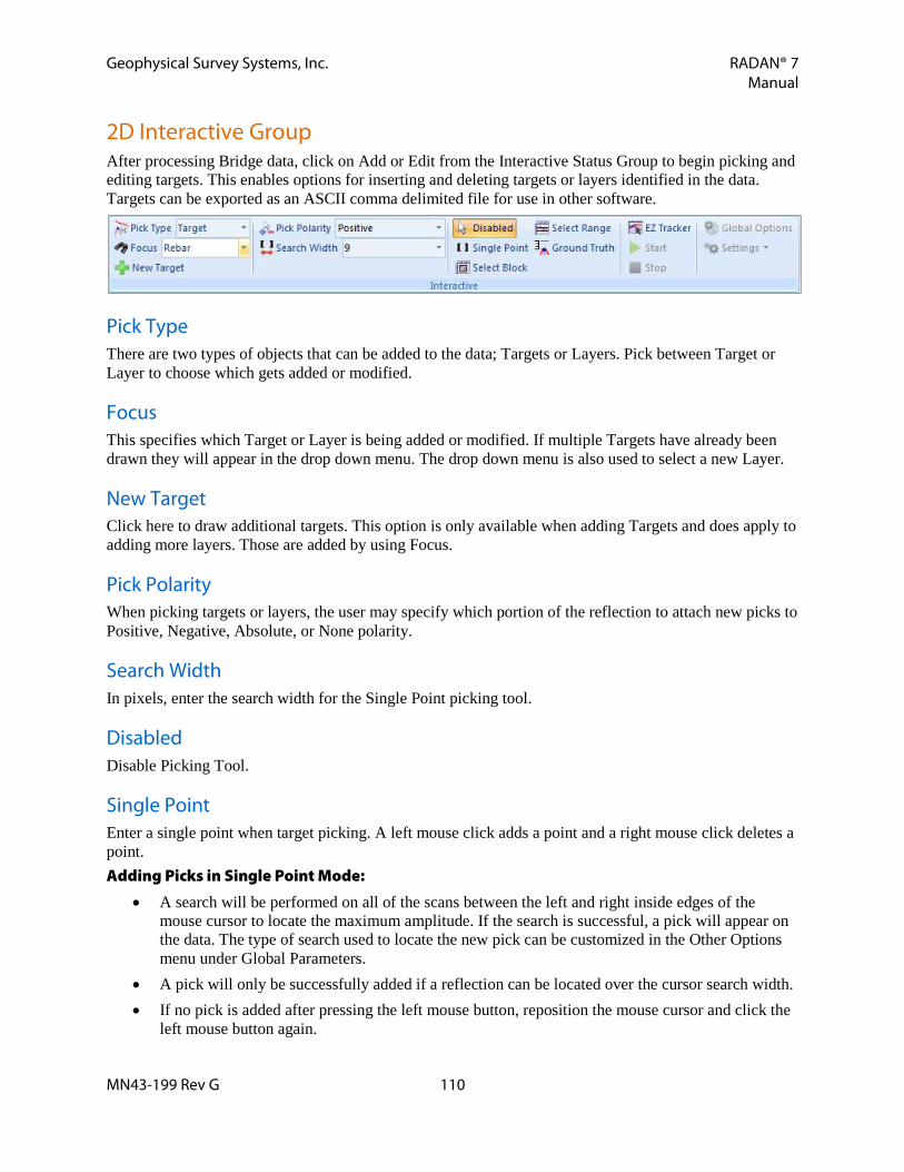
Geophysical Survey Systems, Inc. RADAN® 7 Manual
MN43-199 Rev G 110
2D Interactive Group After processing Bridge data, click on Add or Edit from the Interactive Status Group to begin picking and editing targets. This enables options for inserting and deleting targets or layers identified in the data. Targets can be exported as an ASCII comma delimited file for use in other software.
Pick Type There are two types of objects that can be added to the data; Targets or Layers. Pick between Target or Layer to choose which gets added or modified.
Focus This specifies which Target or Layer is being added or modified. If multiple Targets have already been drawn they will appear in the drop down menu. The drop down menu is also used to select a new Layer.
New Target Click here to draw additional targets. This option is only available when adding Targets and does apply to adding more layers. Those are added by using Focus.
Pick Polarity When picking targets or layers, the user may specify which portion of the reflection to attach new picks to Positive, Negative, Absolute, or None polarity.
Search Width In pixels, enter the search width for the Single Point picking tool.
Disabled Disable Picking Tool.
Single Point Enter a single point when target picking. A left mouse click adds a point and a right mouse click deletes a point. Adding Picks in Single Point Mode:
• A search will be performed on all of the scans between the left and right inside edges of the mouse cursor to locate the maximum amplitude. If the search is successful, a pick will appear on the data. The type of search used to locate the new pick can be customized in the Other Options menu under Global Parameters.
• A pick will only be successfully added if a reflection can be located over the cursor search width. • If no pick is added after pressing the left mouse button, reposition the mouse cursor and click the
left mouse button again.

Geophysical Survey Systems, Inc. RADAN® 7 Manual
MN43-199 Rev G 111
• For cases where the reflection peak is reversed polarity, the user would first need to select Neg. Peak for the Pick Polarity under the Pick Attributes Group, then place the mouse cursor over a negative polarity reflection.
Deleting Picks in Single Point Mode: To delete poor picks, right click on the point with the mouse.
Select Block The Select Block picking tool is designed to operate over a large number of scans. When Select Block is activated a translucent square appears over the data when the user clicks the left mouse button. The select block contains tiny squares on each face and corner for resizing.
Select Range When Select Range is activated a translucent overlay appears over the data, extending the entire length of the profile. It operates similarly to the Select Block, except that all operations performed using the Select Range picking tool are performed within the time interval (slice width) of the selected area on all of the scans in the file. The slice width is adjusted by clicking the left mouse button on one of the handles (located at the top and bottom at the horizontal midpoint of the slice) and dragging the handle to the desired location.
Select Block and Select Range The following options are accessed by right-clicking within the block or range selected. Add Points: Will activate the program to begin a smart search for reflection peaks within the selected region. Circles will overlay the data where reflection peaks are identified by the search algorithm. Picks will be added to whichever Target or Layer is currently active (i.e. in Focus). Delete Points: Will activate the program to start deleting the picks of the current Target or Layer located within the selected region. Pick Modification Options
• Change Pick ID: Change the layer or target number assigned to the picks located within the selected region. For example, the user desires to change the layer # of a group of Layer 3 picks to Layer 2. The user must select layer 3 as the Current Layer, position the Select Block (or Select Range) over the group of points and click the right mouse button to access the Pick Modification Options. Select Change Pick ID to switch from Layer 3 to Layer 2.
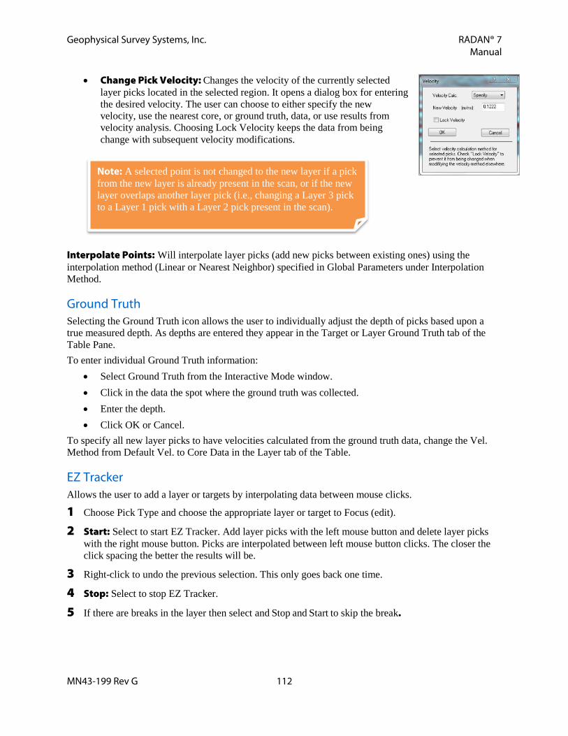
Geophysical Survey Systems, Inc. RADAN® 7 Manual
MN43-199 Rev G 112
• Change Pick Velocity: Changes the velocity of the currently selected layer picks located in the selected region. It opens a dialog box for entering the desired velocity. The user can choose to either specify the new velocity, use the nearest core, or ground truth, data, or use results from velocity analysis. Choosing Lock Velocity keeps the data from being change with subsequent velocity modifications.
Interpolate Points: Will interpolate layer picks (add new picks between existing ones) using the interpolation method (Linear or Nearest Neighbor) specified in Global Parameters under Interpolation Method.
Ground Truth Selecting the Ground Truth icon allows the user to individually adjust the depth of picks based upon a true measured depth. As depths are entered they appear in the Target or Layer Ground Truth tab of the Table Pane. To enter individual Ground Truth information:
• Select Ground Truth from the Interactive Mode window. • Click in the data the spot where the ground truth was collected. • Enter the depth. • Click OK or Cancel.
To specify all new layer picks to have velocities calculated from the ground truth data, change the Vel. Method from Default Vel. to Core Data in the Layer tab of the Table.
EZ Tracker Allows the user to add a layer or targets by interpolating data between mouse clicks.
1 Choose Pick Type and choose the appropriate layer or target to Focus (edit).
2 Start: Select to start EZ Tracker. Add layer picks with the left mouse button and delete layer picks with the right mouse button. Picks are interpolated between left mouse button clicks. The closer the click spacing the better the results will be.
3 Right-click to undo the previous selection. This only goes back one time.
4 Stop: Select to stop EZ Tracker.
5 If there are breaks in the layer then select and Stop and Start to skip the break.
Note: A selected point is not changed to the new layer if a pick from the new layer is already present in the scan, or if the new layer overlaps another layer pick (i.e., changing a Layer 3 pick to a Layer 1 pick with a Layer 2 pick present in the scan).

Geophysical Survey Systems, Inc. RADAN® 7 Manual
MN43-199 Rev G 113
Global Parameters Single Pt. Search Length: When using Single Point Picking Tool, this setting determines whether the pick is entered at the closest peak or using the cursor length. Amplitude Values: Use Data Units, decibels (dB), or Normalized dB.
• Data Units: Provides the layer bottom reflection amplitudes in the actual data values.
• dB: Converts the data units amplitudes to decibels (dB) by using the equation 20*log10(x) where x is the absolute value of the data amplitude.
• Normalized dB: Normalizes the data amplitude relative to 32767 for 16 bit data and 2147483648 for 32 bit data before converting to dB.
Interpolation Method: Each time a pick is added a search is performed to locate the corresponding feature of the reflection that will be used to identify two-way travel time and amplitude. Use either Automatic, Nearest Peak, or Linear.
• Automatic: Performs tracking based on a custom algorithm, which is designed to capture continuous layers that vary with depth. When mouse clicks are spaced more than 20 scans apart this mode switches to Nearest Peak.
• Nearest Peak: Search for the nearest peak between existing picks. • Linear: Draws a straight line between two previously interpreted picks.
Checking the box will fill the layer with a chosen color in depth pane. Click OK or Cancel. Help will open a .pdf of the RADAN 7 manual.
Settings Load Default Settings: Loads previously saved default settings for Interactive Mode. Save As Default Settings: Saves the current Interactive Mode settings including all layer properties and display options.
Non-Filled Layers Filled Layers

Geophysical Survey Systems, Inc. RADAN® 7 Manual
MN43-199 Rev G 114
Export Group Picks may be exported to a comma delimited ASCII (CSV) file, saved as a JPG image file, or the layer information exported to a KML file (if GPS was collected with the data) for viewing in Google Earth.
CSV File Click CSV File to export picks to a comma delimited ASCII file and select which fields to export.
• Use Existing: Use existing custom fields that were created in Create Custom or are available for specific applications from GSSI. o Select an Available Export Configuration. o Modify Options for Filtering Data as necessary. o Save the exported CSV file.
• Create Custom: Select fields to export. o Select the desired Export Category. o Choose which Available Fields to include in the
CSV file. o Choose whether to export all of the data or specify
ranges or certain values. If filtering exported data, then modify Options for Filtering Data as necessary.
o Name the custom export. Create a general name for use with other data.
o Save the exported CSV File. • Modify Existing: Modify an existing field list to create a new one.
o Select an Available Export Configuration. o Select the desired Export Category. o Choose which Available Fields to include in the CSV file. o Choose whether to export all of the data or specify ranges or certain values. If filtering
exported data, then modify Options for Filtering Data as necessary. o Choose whether to output the data at a specific distance interval. o Save the exported CSV File.
• Use Most Recent: Uses the settings from the last used CSV export.
Image Saves the image on the screen as a JPG file. To customize the exported image use the Export > Custom Image Export option under the GSSI Button.

Geophysical Survey Systems, Inc. RADAN® 7 Manual
MN43-199 Rev G 115
KML File A KML file is a file type used to display geographic data in an earth browser, such as Google Earth and Google Maps. KML files have a tag-based structure with names and attributes used for specific display purposes. RADAN 7 can export certain kinds of information as a KML file and easily view that information in Google Earth. This section discusses exporting layers identified in Interactive Interpretation. In order to create a KML file. The data must have been collected with GPS or GPS coordinates were added to the data.
• GPS Track: Select whether or not to export the GPS trajectory. • User Marks: Select whether or not to export User Marks. • Targets: Select whether or not to export Targets. • Ground Truth: Select whether or not to export Ground Truth
points, or Core Data. • Layers: Selects whether or not to export Layers. Multiple layers
are exported one at a time. o Channel: Selects the data channel to export. Different
channels can be exported if a multi-channel file was collected.
o Output Parameter: Select depth, amplitude, velocity, or time depending on the type of data being exported with the layer.
o Line width: The KML output line width in pixels. o Minimum/Maximum: This sets the range of output values specified in the Output Parameter
option. o Number of Intervals: The number of evenly spaced breakpoints for the output data. o View/Edit Layer Colors: Modify the colors applied to each output interval (based upon
Output Parameter and Number of Intervals previously selected). The output of this is a KML file named after the saved data file and the date of the export. To import into Google Earth, simply drag this file onto Planet Earth and it will zoom to the given location of the data.
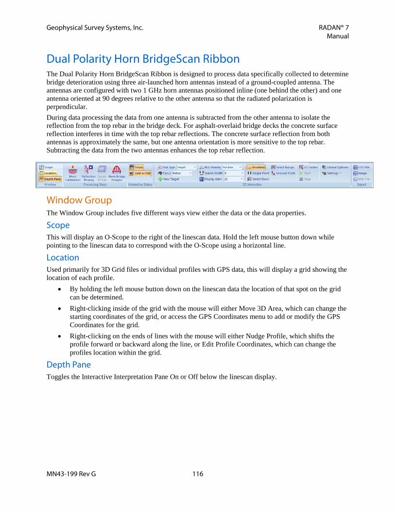
Geophysical Survey Systems, Inc. RADAN® 7 Manual
MN43-199 Rev G 116
Dual Polarity Horn BridgeScan Ribbon The Dual Polarity Horn BridgeScan Ribbon is designed to process data specifically collected to determine bridge deterioration using three air-launched horn antennas instead of a ground-coupled antenna. The antennas are configured with two 1 GHz horn antennas positioned inline (one behind the other) and one antenna oriented at 90 degrees relative to the other antenna so that the radiated polarization is perpendicular. During data processing the data from one antenna is subtracted from the other antenna to isolate the reflection from the top rebar in the bridge deck. For asphalt-overlaid bridge decks the concrete surface reflection interferes in time with the top rebar reflections. The concrete surface reflection from both antennas is approximately the same, but one antenna orientation is more sensitive to the top rebar. Subtracting the data from the two antennas enhances the top rebar reflection.
Window Group The Window Group includes five different ways view either the data or the data properties.
Scope This will display an O-Scope to the right of the linescan data. Hold the left mouse button down while pointing to the linescan data to correspond with the O-Scope using a horizontal line.
Location Used primarily for 3D Grid files or individual profiles with GPS data, this will display a grid showing the location of each profile.
• By holding the left mouse button down on the linescan data the location of that spot on the grid can be determined.
• Right-clicking inside of the grid with the mouse will either Move 3D Area, which can change the starting coordinates of the grid, or access the GPS Coordinates menu to add or modify the GPS Coordinates for the grid.
• Right-clicking on the ends of lines with the mouse will either Nudge Profile, which shifts the profile forward or backward along the line, or Edit Profile Coordinates, which can change the profiles location within the grid.
Depth Pane Toggles the Interactive Interpretation Pane On or Off below the linescan display.

Geophysical Survey Systems, Inc. RADAN® 7 Manual
MN43-199 Rev G 117
Processing Steps Group The Processing Steps Group includes steps for horn calibration, reflection picking, and layer interpretation.
Horn Calibration Settings from the horn calibration are stored with the processed data file header and accessed when the calibration file is used in the reflection picking tool.
1 When the Horn Calibration icon is selected from the Processing Group, the left pane will display the Horn Calibration Process Bar. • Automatic Mode: Perform an automatic horn calibration or choose to
select custom calibration settings. • Use Air Wave File: The airwave file is most commonly collected by
turning the antennas upside down so that they radiate upward. This file is obtained using the same SIR 10/20/30 settings as the metal plate calibration file. Use of an air wave file is optional and not typically used. o No: No air wave file was collected or one is not being used. o Yes: An air wave file has been collected. Enter the air wave filename
in the space to the right. • # of Channels: Number of channels in the data file currently open. • Channel: Choose which channel to calibrate. Setting this to ALL will process all of the channels
with common parameters. o Antenna Type: Select the antenna used for data collection. o Serial Number: Serial number of chosen antenna if it is a Smart antenna.
2 Click Apply and Reset, and adjust if necessary.
3 Click OK once desired results are achieved. It is recommended that the .CZT calibration file is saved with an easily recognizable name to identify it during processing.
Reflection Picking Reflection Picking corrects the ground surface of Horn BridgeScan data based on the previously created Horn Calibration .CZT file. This process eliminates unwanted signal noise to enhance reflections from the pavement layers making them easier to track. Measures the return times of the reflections and calculates the two-way travel time for each of the pavement layers from the data.
1 When the Reflection Picking icon is selected from the Processing Group, the left pane will display the Reflection Picking Process Bar.
Note: RADAN 7 will automatically save the Horn Calibration file to the Proc folder if Auto Save is set to Yes in the Global Parameters.

Geophysical Survey Systems, Inc. RADAN® 7 Manual
MN43-199 Rev G 118
2 Cal(ibration) File Select Method: Select the method for identifying the .CZT, calibration file. • User Select: Manually choose the calibration file. • Current Output Folder: Will search for a .CZT file in the current Output Directory specified in
Global Parameters under the Properties Pane prior to opening any data. • Antenna Database: If there is a serial number and model number an antenna database will
automatically be created. If survey conditions are consistent enough the user does have to recollect a calibration file prior to each survey. Instead the antenna database can be used.
• Auto Select: If Auto Save is set to No it will search the current Output Directory specified in Global Parameters. If the Auto Save is set to Yes it will look in the Proc folder that is automatically created within the Source Directory as specified in Global Parameters. If more than one .CZT is located in the specified folder, RADAN 7 will select the first one in alphanumeric order. If no .CZT file is found it will search the antenna database.
3 Automatic Mode: Select whether or not to use standard settings. If No is selected the following options are available. • Background Removal: Removes horizontal banding in the data. • Starting Depth: Specifies the starting depth for Background Removal. • Apply Inline Position Correction: Correct for inline offset specified in Channel Positions tab
of the Table Pane.
4 Click Apply and Reset, and adjust if necessary.
5 Click OK once desired settings are achieved. RADAN 7 will prompt the user to specify an antenna calibration file.
Create 3D File A step-by-step guide combining collected files, processing the files, and preparing the newly created “bridge” file for further processing. Creation of a 3D file is necessary to complete Bridge Deterioration Mapping, but is not necessary for Bridge QA.
1 Click Create 3D File.
2 Browse to the appropriate folder where the collected bridge files are located.
3 Create an output filename for the newly created bridge 3D file.
4 Click Next.

Geophysical Survey Systems, Inc. RADAN® 7 Manual
MN43-199 Rev G 119
5 Add the bridge files from the left pane to the right pane by: • Double-clicking on the File, or • Click on the File and click Add > , or • If Appropriate, click Add All, or • Highlight a group of files and click Add > • Remove files from the right pane by doing the same
procedures in the right pane
6 Click Next.
7 File Group 3D Area: • Enter the length of the bridge. • Enter the starting distance of the FIRST line collected
from the Curb or Lane Stripe. • Enter the spacing between each profile or line. • Click the down arrow to select how the data were
collected. • Select whether the data were collected Standard or
Inline.
8 Click Next.
9 Adjust File Group Details: Can edit the individual profiles. • Filename: The name of each file collected. • Across Dist.: The distance from the curb of each of
the files collected. • Rev. Dir.: If the files were collected in a zig-zag
pattern and this was specified, an X will automatically be entered that the file will need to be reversed.
• St. Loc.: This is the starting location of the file • Edit St. Loc.: Correct the starting location of the file
as necessary. • End Loc.: This is the ending location of the file. • Edit End Loc.: Correct the ending location of the file
as necessary.
10 Edit the Starting and Ending Locations of each file follow these steps. • Click Edit St. Loc. or Edit End Loc. for EACH file, one at a time. • Move the slider bar until the vertical line on the data matches the beginning of the bridge. This
point will likely correspond with the middle of the bridge joint. Use the left and right arrow keys on the keyboard to make minor adjustments, as well as clicking on the up and down arrows on the screen

Geophysical Survey Systems, Inc. RADAN® 7 Manual
MN43-199 Rev G 120
• Click OK. • Repeat this process for the Starting and Ending Locations for ALL files.
11 Click Next.
12 Enter the Bridge Joint Skew Angle: This will be a positive number if the bridge is angled to the right and negative number if the bridge is angled to the left.
13 Click Finish.
Horn Bridge Analysis This technique locates areas of probable concrete deterioration in a bare concrete or asphalt overlaid concrete deck. This is done by graphing the relative reflection amplitudes across the survey area and assigning threshold values to the amplitude range. Areas of deterioration will attenuate (weaken) the radar signal. This process indicates the presence of deterioration and not the type or cause of that deterioration.
1 When the Deterioration Mapping icon is selected from the Processing Group, the left pane will display the Deterioration Mapping Process Bar.
2 Velocity Calculation: Choose how the radar wave velocity is calculated. • Surface: Select the Surface type of the bridge deck. Either Asphalt
Overlay or Concrete Surface. • Time-Zero Amplitude Threshold: RADAN 7 defaults to the location of
the surface. If this isn’t calculated correctly it can manually be adjusted. • Velocity (Top Layer): RADAN 7 will use the velocity from the File Header
information. If this is incorrect it can manually be adjusted. • Dielectric Constant: This is related to the Velocity and will update as the Velocity if modified.
3 Click Apply and Reset, and adjust if necessary.
4 Click OK once desired results are achieved.

Geophysical Survey Systems, Inc. RADAN® 7 Manual
MN43-199 Rev G 121
Interactive Status Group Show Toggles On or Off the targets and layers already added to the data. Selecting Show does not enable the rest of the 2D Interactive Ribbon. That requires selecting Add or Edit.
Add or Edit When selected the targets or layers already added to the data will be displayed and you can either edit the existing interpretations or add new ones. Selecting Add or Edit enables the rest of the 2D Interactive Ribbon.
2D Interactive Group After processing Bridge data, click on Add or Edit from the Interactive Status Group to begin picking and editing targets. This enables options for inserting and deleting targets or layers identified in the data. Targets can be exported as an ASCII comma delimited file for use in other software.
Pick Type There are two types of objects that can be added to the data; Targets or Layers. Pick between Target or Layer to choose which gets added or modified.
Focus This specifies which Target or Layer is being added or modified. If multiple Targets have already been drawn they will appear in the drop down menu. The drop down menu is also used to select a new Layer.
New Target Click here to draw additional targets. This option is only available when adding Targets and does apply to adding more layers. Those are added by using Focus.
Pick Polarity When picking targets or layers, the user may specify which portion of the reflection to attach new picks to Positive, Negative, Absolute, or None polarity.
Search Width In pixels, enter the search width for the Single Point picking tool.
Disabled Disable Picking Tool.

Geophysical Survey Systems, Inc. RADAN® 7 Manual
MN43-199 Rev G 122
Single Point Enter a single point when target picking. A left mouse click adds a point and a right mouse click deletes a point. Adding Picks in Single Point Mode:
• A search will be performed on all of the scans between the left and right inside edges of the mouse cursor to locate the maximum amplitude. If the search is successful, a pick will appear on the data. The type of search used to locate the new pick can be customized in the Other Options menu under Global Parameters.
• A pick will only be successfully added if a reflection can be located over the cursor search width. • If no pick is added after pressing the left mouse button, reposition the mouse cursor and click the
left mouse button again. • For cases where the reflection peak is reversed polarity, the user would first need to select Neg.
Peak for the Pick Polarity under the Pick Attributes Group, then place the mouse cursor over a negative polarity reflection.
Deleting Picks in Single Point Mode: To delete poor picks, right click on the point with the mouse.
Select Block The Select Block picking tool is designed to operate over a large number of scans. When Select Block is activated a translucent square appears over the data when the user clicks the left mouse button. The select block contains tiny squares on each face and corner for resizing.
Select Range When Select Range is activated a translucent overlay appears over the data, extending the entire length of the profile. It operates similarly to the Select Block, except that all operations performed using the Select Range picking tool are performed within the time interval (slice width) of the selected area on all of the scans in the file. The slice width is adjusted by clicking the left mouse button on one of the handles (located at the top and bottom at the horizontal midpoint of the slice) and dragging the handle to the desired location.
Select Block and Select Range The following options are accessed by right-clicking within the block or range selected. Add Points: Will activate the program to begin a smart search for reflection peaks within the selected region. Circles will overlay the data where reflection peaks are identified by the search algorithm. Picks will be added to whichever Target or Layer is currently active (i.e. in Focus). Delete Points: Will activate the program to start deleting the picks of the current Target or Layer located within the selected region.

Geophysical Survey Systems, Inc. RADAN® 7 Manual
MN43-199 Rev G 123
Pick Modification Options • Change Pick ID: Change the layer or target number assigned to the picks
located within the selected region. For example, the user desires to change the layer # of a group of Layer 3 picks to Layer 2. The user must select layer 3 as the Current Layer, position the Select Block (or Select Range) over the group of points and click the right mouse button to access the Pick Modification Options. Select Change Pick ID to switch from Layer 3 to Layer 2.
• Change Pick Velocity: Changes the velocity of the currently selected layer picks located in the selected region. It opens a dialog box for entering the desired velocity. The user can choose to either specify the new velocity, use the nearest core, or ground truth, data, or use results from velocity analysis. Choosing Lock Velocity keeps the data from being change with subsequent velocity modifications.
Interpolate Points: Will interpolate layer picks (add new picks between existing ones) using the interpolation method (Linear or Nearest Neighbor) specified in Global Parameters under Interpolation Method.
Ground Truth Selecting the Ground Truth icon allows the user to individually adjust the depth of picks based upon a true measured depth. As depths are entered they appear in the Target or Layer Ground Truth tab of the Table Pane. To enter individual Ground Truth information:
• Select Ground Truth from the Interactive Mode window. • Click in the data the spot where the ground truth was collected. • Enter the depth. • Click OK or Cancel.
To specify all new layer picks to have velocities calculated from the ground truth data, change the Vel. Method from Default Vel. to Core Data in the Layer tab of the Table.
EZ Tracker Allows the user to add a layer or targets by interpolating data between mouse clicks.
1 Choose Pick Type and choose the appropriate layer or target to Focus (edit).
2 Start: Select to start EZ Tracker. Add layer picks with the left mouse button and delete layer picks with the right mouse button. Picks are interpolated between left mouse button clicks. The closer the click spacing the better the results will be.
3 Right-click to undo the previous selection. This only goes back one time.
Note: A selected point is not changed to the new layer if a pick from the new layer is already present in the scan, or if the new layer overlaps another layer pick (i.e., changing a Layer 3 pick to a Layer 1 pick with a Layer 2 pick present in the scan).

Geophysical Survey Systems, Inc. RADAN® 7 Manual
MN43-199 Rev G 124
4 Stop: Select to stop EZ Tracker.
5 If there are breaks in the layer then select and Stop and Start to skip the break.
Global Parameters Single Pt. Search Length: When using Single Point Picking Tool, this setting determines whether the pick is entered at the closest peak or using the cursor length. Amplitude Values: Use Data Units, decibels (dB), or Normalized dB.
• Data Units: Provides the layer bottom reflection amplitudes in the actual data values.
• dB: Converts the data units amplitudes to decibels (dB) by using the equation 20*log10(x) where x is the absolute value of the data amplitude.
• Normalized dB: Normalizes the data amplitude relative to 32767 for 16 bit data and 2147483648 for 32 bit data before converting to dB.
Interpolation Method: Each time a pick is added a search is performed to locate the corresponding feature of the reflection that will be used to identify two-way travel time and amplitude. Use either Automatic, Nearest Peak, or Linear.
• Automatic: Performs tracking based on a custom algorithm, which is designed to capture continuous layers that vary with depth. When mouse clicks are spaced more than 20 scans apart this mode switches to Nearest Peak.
• Nearest Peak: Search for the nearest peak between existing picks. • Linear: Draws a straight line between two previously interpreted picks.
Checking the box will fill the layer with a chosen color in depth pane. Click OK or Cancel. Help will open a .pdf of the RADAN 7 manual.
Settings Load Default Settings: Loads previously saved default settings for Interactive Mode. Save As Default Settings: Saves the current Interactive Mode settings including all layer properties and display options.
Non-Filled Layers Filled Layers

Geophysical Survey Systems, Inc. RADAN® 7 Manual
MN43-199 Rev G 125
Export Group Picks may be exported to a comma delimited ASCII (CSV) file, saved as a JPG image file, or the layer information exported to a KML file (if GPS was collected with the data) for viewing in Google Earth.
CSV File Click CSV File to export picks to a comma delimited ASCII file and select which fields to export.
• Use Existing: Use existing custom fields that were created in Create Custom or are available for specific applications from GSSI. o Select an Available Export Configuration. o Modify Options for Filtering Data as necessary. o Save the exported CSV file.
• Create Custom: Select fields to export. o Select the desired Export Category. o Choose which Available Fields to include in the
CSV file. o Choose whether to export all of the data or
specify ranges or certain values. If filtering exported data, then modify Options for Filtering Data as necessary.
o Name the custom export. Create a general name for use with other data.
o Save the exported CSV File. • Modify Existing: Modify an existing field list to create a new one.
o Select an Available Export Configuration. o Select the desired Export Category. o Choose which Available Fields to include in the CSV file. o Choose whether to export all of the data or specify ranges or certain values. If filtering
exported data, then modify Options for Filtering Data as necessary. o Choose whether to output the data at a specific distance interval. o Save the exported CSV File.
• Use Most Recent: Uses the settings from the last used CSV export.
Image Saves the image on the screen as a JPG file. To customize the exported image use the Export > Custom Image Export option under the GSSI Button.

Geophysical Survey Systems, Inc. RADAN® 7 Manual
MN43-199 Rev G 126
KML File A KML file is a file type used to display geographic data in an earth browser, such as Google Earth and Google Maps. KML files have a tag-based structure with names and attributes used for specific display purposes. RADAN 7 can export certain kinds of information as a KML file and easily view that information in Google Earth. This section discusses exporting layers identified in Interactive Interpretation. In order to create a KML file. The data must have been collected with GPS or GPS coordinates were added to the data.
• GPS Track: Select whether or not to export the GPS trajectory. • User Marks: Select whether or not to export User Marks. • Targets: Select whether or not to export Targets. • Ground Truth: Select whether or not to export Ground Truth
points, or Core Data. • Layers: Selects whether or not to export Layers. Multiple layers
are exported one at a time. o Channel: Selects the data channel to export. Different
channels can be exported if a multi-channel file was collected. o Output Parameter: Select depth, amplitude, velocity, or time depending on the type of data
being exported with the layer. o Line width: The KML output line width in pixels. o Minimum/Maximum: This sets the range of output values specified in the Output Parameter
option. o Number of Intervals: The number of evenly spaced breakpoints for the output data. o View/Edit Layer Colors: Modify the colors applied to each output interval (based upon
Output Parameter and Number of Intervals previously selected). The output of this is a KML file named after the saved data file and the date of the export. To import into Google Earth, simply drag this file onto Planet Earth and it will zoom to the given location of the data.

Geophysical Survey Systems, Inc. RADAN® 7 Manual
MN43-199 Rev G 127
Google Earth® Ribbon The Google Earth® Ribbon provides viewing and exporting options for data collected with GPS. Options include viewing GPS Tracks, User Marks, Layers, Targets, and Ground Truth in Google Earth, exporting to a KML file, and launching and refreshing Google Earth®.
Display/Save Options Group There are three options in this group for saving or displaying export items in Google Earth®. KML File: Click this button to save selected export items to a KML File. A KML file is a file type used to display geographic data in an earth browser, such as Google Earth® and Google Maps®. KML files have a tag-based structure with names and attributes used for specific display purposes. Google Earth®: Click this button to launch Google Earth® with the selected export options. A Temporary Place will be added to Google Earth®. Google Earth® Refresh: Press this button to refresh Google Earth® with any changes made to the exported items. A new Temporary Place will be added to Google Earth® and will have the same file name as the original file.
Export Items Group This group allows the user to choose which items will be exported as part of a KML file. Only the displayed layers and targets associated with the displayed channel are exported. Layers: Currently displayed layer(s). Select which Layer(s) is displayed by checking the Display box in the Layers Tab of the Table. Targets: Currently displayed target(s). Select which Target(s) is displayed by checking the Display box in the Targets Tab of the Table. User Marks: Export User Marks as they appear in the Way Points Tab of the Table. GPS Path: The GPS Path associated with Channel 1. Ground Truth: Currently displayed Ground Truth data for Layers or Targets.
Layer Options Group This group allows the user to customize how the displayed layers are exported. Output Parameter: There are four Output Parameter options to choose from when exporting layers. Although depth is the typical output parameter, there are applications where other values such as velocity (e.g. new pavement) or amplitude (e.g. bridge deck) provide valuable information.
• Depth • Amplitude • Velocity • Time
Note: Google Earth® must be installed on the user’s computer for either the Google Earth® or the Google Earth® Refresh icons to work.

Geophysical Survey Systems, Inc. RADAN® 7 Manual
MN43-199 Rev G 128
Line Width: Display width of the line in Google Earth®. Number of Intervals: Exported values can be broken into different colors to denote different ranges. The user can specify from 0 to 8 intervals. Minimum Value: The minimum value for the interval range. For example, if the user choses Amplitude for the output parameter, the Minimum Value is the minimum amplitude. Maximum Value: The maximum value for the interval range. For example, if the user choses Amplitude for the output parameter, the Maximum Value is the maximum amplitude. Interval Colors: Opens the Interval Colors dialogue box, which allows the user to select a color for each interval. Click on the down arrows to select a different color or choose Other to open a color editor window.
Settings Group Recall Settings: Press this button to recall the current export settings (Export Items and Layer Options) that have most recently been saved by pressing the Save Settings icon. Save Settings: Press this button to save the current export settings (Export Items and Layer Options) as the default settings for all files.
3D Volume Options This is a context sensitive ribbon that will only be accessible when 3D data is displayed and selected as the active dataset.
3D Slice Controls Group Select X, Y, or Z to focus on either a profile or the slice when manipulating the 3D display. This will also update as different axes are selected from other groups. Bookmark: Bookmark individual X-walls, Y-walls, or Z-slices.
eReset: Reset the image to original slice settings.
Note: Thickness settings do not apply to bookmarked walls or slices. This may affect how the bookmark appears after it is placed.

Geophysical Survey Systems, Inc. RADAN® 7 Manual
MN43-199 Rev G 129
3D Slice Viewpoint Settings: These functions are applied by holding down the X, Y, or Z key on the keyboard or by selecting the appropriate wall or slice from the 3D Slice Control options.
Expand View: Expand the 3D image in the X, Y, or Z direction. Decrease View: Contract the 3D image in the X, Y, or Z direction. Viewpoint Reset: Snap back to the original size.
Viewpoint Group Pan: Click here, move the mouse pointer (represented as a hand) to the 3D image. Then while holding down the left mouse button, move the image. Zoom: Click here, move the mouse point (represented as a magnifying glass) to the 3D image. Control the size of the zoom by moving the wheel on the mouse. Double-click to zoom in on the square area. Rotate: Click here to select the rotation for the 3D Cube.
• Use the arrows or enter the numeric angle to rotate, or spin, the image on the X, Y, or Z axis.
• Toggle with a check mark to Apply Immediately. • Click Apply to test the settings without exiting, click Done to apply the
changes and exit, or Cancel to exit without applying the changes. Help will open a .pdf of the RADAN 7 manual.
• To view just the Z-slice data change the settings to X = 90, Y = 0, and Z = 0.
3D Show/Hide Group Points: Toggle to show or hide points (targets) entered in the 3D Data using Interactive Mode. Lines: Toggle to show or hide lines (pipes, rebar, etc.) entered in the 3D Data using Interactive Mode. Waypoints: Toggle to show or hide waypoints (User Marks or Computer Generated Marks). sContours: Toggle to show or hide an amplitude contour of the 3D Data. Shown in the image on the right. The contour image is updated as the Z Slice is moved. Surfaces: Toggle to show or hide surfaces of the 3D Data. Surfaces are added by importing a .shp file under 3D Display Properties in the Properties Pane. Slices: Toggle to show or hide all of the X, Y, and Z slices of the 3D Data.
Note: Click the Viewpoint Reset icon to return to the original image.

Geophysical Survey Systems, Inc. RADAN® 7 Manual
MN43-199 Rev G 130
X-Slice and Y-Slice Groups X/Y-Slice Position: Drag the slide bar or press the -/+ to move the profiles of the 3D display. Animation: Toggles animation On or Off. This will seamlessly move through the profiles.
Z-Slice Group Z-Slice Position: Drag the slide bar or press the -/+ to move the slices of the 3D display. Animation: Toggles animation On or Off. This will seamlessly move through the profiles. Thickness: Adjust the thickness of the Z-Slice.
3D Interactive Group Disabled: Turns off Interactive Mode. Free Draw: Draw rebar, pipes, conduits, etc. at the location of the current Z Slice. Steps on how to draw a pipe are below.
1 Double click on the location for the beginning of the pipe.
2 Double click on the location for the end of the pipe.
3 To create additional pipes choose New Object from the Free Draw window or right click within the 3D cube and select New Target.
Snap to Data: Draws targets and attaches them to the nearest scan and not the Z Slice.
1 Double click to on the location for the beginning of the pipe.
2 Double click for on the location of the end of the pipe.
3 To create additional pipes choose New Target from the Interactive window or right click within the 3D cube and select New Target.
Focus: In Free Draw mode, this specifies the object that is being entered or modified. If multiple objects have already been drawn they will appear in the drop down menu. New Target: Click here to draw additional objects.
Export Group Picks may be exported to a comma delimited ASCII (CSV) file, saved as a JPG image file, or the layer information exported to a KML file (if GPS was collected with the data) for viewing in Google Earth. JPG: Click to export the 3D grid to a JPG file. Excel: Opens a dialogue box to enter project information. Then create a report in Microsoft Excel with user-entered information, data properties, and an image of the currently selected view. 2D CAD (*.dxf): Exports the data as a 2D AutoCAD file. 3D CAD (*.dxf): Exports the data as a 3D AutoCAD file. Z-Slice Google Earth (*.kml): Exports the currently displayed z-slice as a kml file that will open in Google Earth as a layer.

Geophysical Survey Systems, Inc. RADAN® 7 Manual
MN43-199 Rev G 131
Section 4: Application-Specific Displays
Reader Use this display to view already processed 2D data as profiles and 3D data as depth slices. The color table, color transform, and display gain can also be modified. If targets or picks were added in one of the other displays they can be displayed as well. Displayed data can be saved as .jpg images.
GSSI Button Clicking on the GSSI Button allows the user to:
• Open a File/Project • Print data • Close a File/Project • Close All Open Files • Options to change languages • Exit RADAN 7 Software

Geophysical Survey Systems, Inc. RADAN® 7 Manual
MN43-199 Rev G 132
GPR Reader – View Processed Data and Interactive Edits
File Group Open: Opens the currently selected project folder to open additional files. Close: Closes the currently selected data file. If multiple files are open it closes the tab that is active.
Interactive Status Show: Toggles On or Off the targets and layers already added to the data.
Export 2D JPG: Click to export the 3D grid to a JPG file.
Depth Slice Viewing View Depth Slices Display a top-down view of data and slice through difference depths.
Other Windows Group Toggle On or Off different data property windows. Location Used primarily for 3D Grid files or individual profiles with GPS data, location will display a grid showing the location of each profile.
• Holding the left mouse button down on the linescan data will show the location of that spot on the location display.
• Right-click with the mouse inside of the location display to access the following: o Move 3D Area: Change the starting
coordinates of the grid. o GPS Coordinates: Add or modify the GPS Coordinates for the grid.
• Right-click with the mouse on the end of a line to access the following: o Nudge Profile: Shift the profile forward or backward along the line. o Edit Profile Coordinates: Change a profile’s location within the grid.
File Header: Header information about the displayed file. Global Settings: Display Global Parameters for all files in a particular project prior to opening any files and allow you to switch between available Application Displays. Once a file is open, the Global Parameters cannot be changed.

Geophysical Survey Systems, Inc. RADAN® 7 Manual
MN43-199 Rev G 133
Display Group Color Tables Color tables are used to code the amplitude of each scan (i.e., the recorded radar signal). Colors on the left side of the spectrum represent strong negative amplitudes. As the colors go to the right, this represents the amplitude getting weaker (or closer to 0) and the middle of the spectrum is the area of weak amplitude. As the colors go further right from the middle, this represents a stronger positive amplitude.
• For example, white in color table 1 corresponds to the highest positive amplitude pulse; therefore, when it appears on the radar record, it means that there is a strong reflection (or a high dielectric contrast).
• In some color tables (such as 23), black indicates a low amplitude reflection. Therefore, a large black region on the linescan plot could be indicative of a uniform structure (such as a homogeneous sand deposit) with little or no dielectric contrast.
Color Xforms The Color Transform can be changed to enhance weak amplitude or small contrast reflectors. The color transform determines whether the color scale applied to the radar wave’s amplitude is linear, logarithmic, exponential, or customized. This function can also be used to de-emphasize certain features.
Display Gain To change the Display Gain, click Display Gain in the Home Ribbon or right-click on the data window and select Display Gain. Then select from a preset list of multiples ranging from -6 up to 60. Input a Custom Value by right-clicking and selecting Custom from Display Gain menu. This will change all samples, no matter where they are in the scan trace, by the same amount.
• Altering the display gain does not change data values like Range Gain, which is described later in this section under the Easy Processing and Processing sections.
• Altering the display gain may make it easier to see lower amplitude targets.
Help Index: Opens the RADAN for StructureScan Mini Manual. About: Display the current version of the software. Update: Update the software to the latest version. You MUST be connected to the internet to do this.
Note: There are 30 different color tables and RADAN defaults to True Grey 17. There are 20 color transforms and
RADAN defaults to Linear Transform 3.

Geophysical Survey Systems, Inc. RADAN® 7 Manual
MN43-199 Rev G 134
Depth Slice Options This is a context sensitive ribbon that will only be accessible when 3D data is displayed and selected as the active dataset.
Z-Slice Group Z-Slice Position: Drag the slide bar or press the -/+ to move the slices of the 3D display. Animation: Toggles animation On or Off. This will seamlessly move through the profiles. Thickness: Adjust the thickness of the Z-Slice.
Standard Processing See Section 3: Navigating Through RADAN 7 for the complete overview of Standard Processing.

Geophysical Survey Systems, Inc. RADAN® 7 Manual
MN43-199 Rev G 135
RADAN 7 for StructureScan Mini RADAN for StructureScan Mini display was designed to process, view, and document data collected with the StructureScan Mini. RADAN for StructureScan Mini module can perform the following functions: Process data using Focus (Migration), Background Removal, and Gain Adjustment; Display 3D images and provide X,Y, and Z coordinates; Change colors to optimize images for documentation purposes; Add interpretations to the data; Export information to MSExcel for reports; Export a 3D image as a JPG file; and Export target information to a CSV format.
GSSI Button Clicking on the button allows you to:
• Open a File/Project • Print your data • Close a File/Project • Close All Open Files • Open a previously processed File/Project • Use Options to change the language • Exit RADAN for StructureScan Mini Software

Geophysical Survey Systems, Inc. RADAN® 7 Manual
MN43-199 Rev G 136
RADANMini Home Ribbon
File Group Open: Opens the currently selected project folder to open additional files. Save: Saves the selected data file. If multiple files are open it saves the tab that is active. Any new targets or picks added to the data will be saved. Close: Closes the currently selected data file. If multiple files are open it closes the tab that is active.
Processing Options Group Focus When the software automatically processes your data, it will use the dielectric number you configured and used when the data were collected. This value may or may not give you the optimum 3D display. The objects displayed in the 3D view may look blurred or blobby. You can use the Focus option to re-adjust the dielectric for better depth accuracy and a better 3D display.
1 Close the 3D Tab by clicking on the X of the tab so only the original file tab remains.
2 Click on Focus
3 Adjust the slider bar to increase or decrease the velocity (thus increase or decrease the dielectric) and click on the Test Icon
4 Continue to make adjustments and press the Test Icon until the hyperbolas become dots. • The picture on the left has hyperbolas. Increase the velocity bar by
sliding it to the right. This will automatically decrease the dielectric.

Geophysical Survey Systems, Inc. RADAN® 7 Manual
MN43-199 Rev G 137
• The picture in the middle has upside-down hyperbolas. Decrease the velocity by sliding it to the left. This will automatically increase the dielectric.
• The picture on the right has no hyperbolas. Dots are present.
5 Click on the Process Icon to process the data.
6 Save the data if prompted to do so.
Background Removal Remove any background noise your data may have. Clicking on this icon will immediately begin the process. Save the file if prompted.
Data Windows Group Scope: Toggle on and off to display the O-Scope RADAR signal. (You may hold the left mouse button down on the data and move the mouse to view the RADAR signal at that position. 3D View: Toggle between displaying the 3D Grid view.

Geophysical Survey Systems, Inc. RADAN® 7 Manual
MN43-199 Rev G 138
Other Windows Group Toggle On or Off different data property windows. File Header: Header information about the displayed file. Global Settings: Display Global Parameters for all files in a particular project prior to opening any files and allow you to switch between available Application Displays. Once a file is open, the Global Parameters cannot be changed. Window Settings: The Properties Pane automatically updates based on which data display, 2D or 3D is currently selected.
Interactive 2D Group Perform the following steps on the 2D profile and not on the 3D View. Add/Del Targets: This will allow you to “tag” targets with a dot. Simply turn this on and click on a target to insert a dot. Right click on a dot to delete the dot. These dots will contain information about the target such a horizontal distance, depth, and velocity. The information can be exported as a comma delimited ASCII file. Also, note that the dots will appear on the 3D Grid as well. Edit Targets: This will allow you to click on a dot to change the color and size of the dot. Ground Truth: This will allow you to click on a target and enter the KNOWN DEPTH of that target. This will adjust the scale accordingly.
Display Options Group Color Tables: Change the color of your data. Color Xforms: Change how the colors of your chosen color table is distributed. Display Gain: Change the contrast (brightness) of your data. This changes the display only; it does not change the actual data. Targets: Turn the display of the targets (dots) on or off.

Geophysical Survey Systems, Inc. RADAN® 7 Manual
MN43-199 Rev G 139
Export 2D Group Targets: Export targets (dots) information (distance, depth and layer velocity) to a comma delimited ASCII file. The name of the file is “FileName”+”X”.csv located in the output folder. JPEG: Save the current file as a JPEG file (Picture File). This file will be named “FileName”+”X”.jpg located in the output folder. Excel: Create a report in MSExcel with user entered information, data information and a picture of the 3D Grid.
1 Enter information if needed. Click on OK when done.
2 Open the Excel by clicking at the bottom of the screen if it did not automatically open.
3 In Excel move the picture and adjust the size of the picture as needed.
4 Print the report.
Clipboard Copy: Click this to copy the current file to the clipboard. This image then can be pasted to any other 3rd party software (PowerPoint, Word, etc.).
Print Quick Print: Print the image as is. Setup: Configure the printout.
• Scan Per Inch: Number of scans per inch.
• Print Page Headers: Print Header information.
• Continuous Page: If data takes more than one page, print data on multiple pages or one page.
• Load Logo: Load and print your own logo, or GSSI logo.
Help Index: Opens the RADAN for StructureScan Mini Manual. About: Display the current version of the software. Update: Update the software to the latest version. You MUST be connected to the internet to do this.

Geophysical Survey Systems, Inc. RADAN® 7 Manual
MN43-199 Rev G 140
3D Volume Options Ribbon
X-Slice, Y-Slice, Z-Slice Groups Drag the slide bar or press the to move the slices of the 3D Grid according. You may also animate the slices individually by clicking on the Animation icon. This icon will turn animation on and off Thickness (Z-Slice): Adjust the thickness of the Z-Slice.
View Options Group Targets: Toggle between displaying the targets. GPR Data: Toggle between displaying the data of the 3D Grid. Display Gain: Adjust the display gain (contrast). Background: Toggle between a black background and white background.
Export Group JPG: Export the 3D grid as a JPG file. Excel: Create a report in MSExcel with user entered information, data information and a picture of the 3D Grid. Use the same steps described above in the RADANMini Home Ribbon section. 2D CAD (*.dxf): Exports the data as a 2D AutoCAD file. 3D CAD (*.dxf): Exports the data as a 3D AutoCAD file. Z-Slice Google Earth (*.kml): Exports the currently displayed z-slice as a kml file that will open in Google Earth as a layer.

Geophysical Survey Systems, Inc. RADAN® 7 Manual
MN43-199 Rev G 141
UtilityScan DF The UtilityScan DF display was designed to process, view, and document data collected with the UtilityScan DF (dual frequency) system. This module can perform the following functions: Process data using Focus (Migration), Background Removal, Gain Adjustment, Maximum Depth, and Channel Blending; Display 3D images and provide X,Y, and Z coordinates; Change colors to optimize images for documentation purposes; Add interpretations to the data; Export information to MSExcel for reports; Export a 3D image as a JPG file; and Export target information to a CSV format.
GSSI Button Clicking on the button allows you to:
• Open a File/Project • Print your data • Close a File/Project • Close All Open Files • Open a previously processed File/Project • Use Options to change the language • Exit RADAN for StructureScan Mini Software

Geophysical Survey Systems, Inc. RADAN® 7 Manual
MN43-199 Rev G 142
UtilityScan DF Applications Ribbon
File Group Open: Opens the currently selected project folder to open additional files. Save: Saves the selected data file. If multiple files are open it saves the tab that is active. Any new targets or picks added to the data will be saved. Close: Closes the currently selected data file. If multiple files are open it closes the tab that is active.
Processing Options Group Channel Blending The Channel Blending function serves to blend two separate channels of data into one profile. When the Channel Blending icon is selected it blends the two channels of data together using an 80% position on Channel 1 and a 20% blending width.
Prior to Channel Blending.
Note: The output from Channel Blending is placed in Channel 2 and replaces the original Channel 2 data. The first channel of data is still available in Channel 1.

Geophysical Survey Systems, Inc. RADAN® 7 Manual
MN43-199 Rev G 143
Following Channel Blending.
Focus When the software automatically processes your data, it will use the dielectric number you configured and used when the data were collected. This value may or may not give you the optimum 3D display. The objects displayed in the 3D view may look blurred or blobby. You can use the Focus option to re-adjust the dielectric for better depth accuracy and a better 3D display.
1 Close the 3D Tab by clicking on the X of the tab so only the original file tab remains.

Geophysical Survey Systems, Inc. RADAN® 7 Manual
MN43-199 Rev G 144
2 Click on Focus
3 Adjust the slider bar to increase or decrease the velocity (thus increase or decrease the dielectric) and click on the Test Icon
4 Continue to make adjustments and press the Test Icon until the hyperbolas become dots. • The picture on the left has hyperbolas. Increase the velocity bar by
sliding it to the right. This will automatically decrease the dielectric. • The picture in the middle has upside-down hyperbolas. Decrease the velocity by sliding it to the
left. This will automatically increase the dielectric. • The picture on the right has no hyperbolas. Dots are present.
5 Click on the Process Icon to process the data.
6 Save the data if prompted to do so.
Background Removal Remove any background noise your data may have. Clicking on this icon will immediately begin the process. Save the file if prompted.

Geophysical Survey Systems, Inc. RADAN® 7 Manual
MN43-199 Rev G 145
Signal Floor This function analyzes the noise and signal loss (attenuation) from scan to scan and provides estimate of the effective depth penetration. Real reflectors may still be located beneath the Signal Floor if they are strong enough. The output of this function is shown as a green line on the screen, as seen below, and saved as a .BII binary file.
1 When the Max Depth icon is clicked, the left pane will display the Signal Floor Process Bar.
2 Signal Floor Estimator: If multiple channels of data were collected, choose between which channels to use to estimate max depth.
3 Simply click Apply and Reset to test this processing function. Click OK to accept the setting and generate the binary file.
Data Windows Group Scope: Toggle on and off to display the O-Scope RADAR signal. (You may hold the left mouse button down on the data and move the mouse to view the RADAR signal at that position. 3D View: Toggle between displaying the 3D Grid view. Location: Used primarily for 3D Grid files or individual profiles with GPS data, location will display a grid showing the location of each profile.
Other Windows Group Toggle On or Off different data property windows. File Header: Header information about the displayed file. Global Settings: Display Global Parameters for all files in a particular project prior to opening any files and allow you to switch between available Application Displays. Once a file is open, the Global Parameters cannot be changed. Window Settings: The Properties Pane automatically updates based on which data display, 2D or 3D is currently selected. Tables: This pane will display database information about the currently active file. Tabs are displayed depending on the type of application or process underway.
Interactive 2D Perform the following steps on the 2D profile and not on the 3D View. Add/Del Targets: This will allow you to tag targets with a dot. Simply turn this on and click on a target to insert a dot. Right click on a dot to delete the dot. These dots will contain information about the target such a horizontal distance, depth, and velocity. The information can be exported as a comma delimited ASCII file. Also, note that the dots will appear on the 3D Grid as well.

Geophysical Survey Systems, Inc. RADAN® 7 Manual
MN43-199 Rev G 146
Edit Targets: This will allow you to click on a dot to change the color and size of the dot. Ground Truth: This will allow you to click on a target and enter the KNOWN DEPTH of that target. This will adjust the scale accordingly.
Display Options Color Tables: Change the color of your data. Color Xforms: Change how the colors of your chosen color table is distributed. Display Gain: Change the contrast (brightness) of your data. This changes the display only; it does not change the actual data. Targets: Turn the display of the targets (dots) on or off. Max Depth: Toggles Max Depth On or Off.
Export 2D Targets: Export targets (dots) information (distance, depth and layer velocity) to a comma delimited ASCII file. The name of the file is “FileName”+”X”.csv located in the output folder. JPEG: Save the current file as a JPEG file (Picture File). This file will be named “FileName”+”X”.jpg located in the output folder. Excel: Create a report in MSExcel with user entered information, data information and a picture of the 3D Grid.
1 Enter information if needed. Click on OK when done.
2 Open the Excel by clicking at the bottom of the screen if it did not automatically open.
3 In Excel move the picture and adjust the size of the picture as needed.
4 Print the report.
Clipboard Copy: Click this to copy the current file to the clipboard. This image then can be pasted to any other 3rd party software (PowerPoint, Word, etc.).
Print Quick Print: Print the image as is. Setup: Configure the printout.
• Scan Per Inch: Number of scans per inch • Print Page Headers: Print Header information • Continuous Page: If data takes more than one page, print
data on multiple pages or one page • Load Logo: Load and print your own logo, or GSSI logo

Geophysical Survey Systems, Inc. RADAN® 7 Manual
MN43-199 Rev G 147
Help Index: Opens the RADAN for StructureScan Mini Manual. About: Display the current version of the software. Update: Update the software to the latest version. You MUST be connected to the internet to do this.
Google Earth® Ribbon The Google Earth® Ribbon provides viewing and exporting options for data collected with GPS. Options include viewing GPS Tracks, User Marks, Layers, Targets, and Ground Truth in Google Earth, exporting to a KML file, and launching and refreshing Google Earth®.
Display/Save Options Group There are three options in this group for saving or displaying export items in Google Earth®. KML File: Click this button to save selected export items to a KML File. A KML file is a file type used to display geographic data in an earth browser, such as Google Earth® and Google Maps®. KML files have a tag-based structure with names and attributes used for specific display purposes. Google Earth®: Click this button to launch Google Earth® with the selected export options. A Temporary Place will be added to Google Earth®. Google Earth® Refresh: Press this button to refresh Google Earth® with any changes made to the exported items. A new Temporary Place will be added to Google Earth® and will have the same file name as the original file.
Export Items Group This group allows the user to choose which items will be exported as part of a KML file. Only the displayed layers and targets associated with the displayed channel are exported. Layers: Currently displayed layer(s). Select which Layer(s) is displayed by checking the Display box in the Layers Tab of the Table. Targets: Currently displayed target(s). Select which Target(s) is displayed by checking the Display box in the Targets Tab of the Table. User Marks: Export User Marks as they appear in the Way Points Tab of the Table. GPS Path: The GPS Path associated with Channel 1. Ground Truth: Currently displayed Ground Truth data for Layers or Targets.
Layer Options Group This group allows the user to customize how the displayed layers are exported.
Note: Google Earth® must be installed on the user’s computer for either the Google Earth® or the Google Earth® Refresh icons to work.

Geophysical Survey Systems, Inc. RADAN® 7 Manual
MN43-199 Rev G 148
Output Parameter: There are four Output Parameter options to choose from when exporting layers. Although depth is the typical output parameter, there are applications where other values such as velocity (e.g. new pavement) or amplitude (e.g. bridge deck) provide valuable information.
• Depth • Amplitude • Velocity • Time
Line Width: Display width of the line in Google Earth®. Number of Intervals: Exported values can be broken into different colors to denote different ranges. The user can specify from 0 to 8 intervals. Minimum Value: The minimum value for the interval range. For example, if the user choses Amplitude for the output parameter, the Minimum Value is the minimum amplitude. Maximum Value: The maximum value for the interval range. For example, if the user choses Amplitude for the output parameter, the Maximum Value is the maximum amplitude. Interval Colors: Opens the Interval Colors dialogue box, which allows the user to select a color for each interval. Click on the down arrows to select a different color or choose Other to open a color editor window.
Settings Group Recall Settings: Press this button to recall the current export settings (Export Items and Layer Options) that have most recently been saved by pressing the Save Settings icon. Save Settings: Press this button to save the current export settings (Export Items and Layer Options) as the default settings for all files.
3D Volume Options Ribbon
X-Slice, Y-Slice, Z-Slice Groups Drag the slide bar or press the to move the slices of the 3D Grid according. You may also animate the slices individually by clicking on the Animation icon. This icon will turn animation on and off Thickness (Z-Slice): Adjust the thickness of the Z-Slice
View Options Group Targets: Toggle between displaying the targets. GPR Data: Toggle between displaying the data of the 3D Grid Display Gain: Adjust the display gain (contrast) Background: Toggle between a black background and white background.

Geophysical Survey Systems, Inc. RADAN® 7 Manual
MN43-199 Rev G 149
Export Group JPG: Export the 3D grid as a JPG file Excel: Create a report in MSExcel with user entered information, data information and a picture of the 3D Grid. Use the same steps described above in the RADANMini Home Ribbon section. 2D CAD (*.dxf): Exports the data as a 2D AutoCAD file. 3D CAD (*.dxf): Exports the data as a 3D AutoCAD file. Z-Slice Google Earth (*.kml): Exports the currently displayed z-slice as a kml file that will open in Google Earth as a layer.

Geophysical Survey Systems, Inc. RADAN® 7 Manual
MN43-199 Rev G 150
RoadScan Provides viewing and processing options for data collected specifically for determining pavement layer thickness.
GSSI Button Clicking on the GSSI Button allows the user to:
• Open a File/Project • Assemble Files • Import GPS • Save a File/Project • Save As a File/Project under a different name or
format • Export data • Print data • Close a File/Project • Close All Open Files • Open a previously processed File/Project • Options to change languages • Exit RADAN 7 Software

Geophysical Survey Systems, Inc. RADAN® 7 Manual
MN43-199 Rev G 151
Home Ribbon
File Group Open: Opens the currently selected project folder to open additional files. Save: Saves the selected data file. If multiple files are open it saves the tab that is active. Any new targets or picks added to the data will be saved. Close: Closes the currently selected data file. If multiple files are open it closes the tab that is active.
Data Windows Group LineScan In the linescan display data are displayed in a color-amplitude form, where a color is assigned to a specific positive or negative amplitude value of the recorded signal dependent upon the color table and color transform selected. The vertical scale represents time (or depth) while the horizontal scale represents the horizontal distance traveled by the radar antenna. The Linescan display is the most useful for mapping man-made objects, such as underground storage tanks, pipes, and drums or for mapping geologic layers.
Scope This will display an O-Scope to the right of the linescan data. Hold the left mouse button down while pointing to the linescan data to correspond the same point with the O-Scope using a horizontal line.
3D View This will display the data as a 3D Cube. More information and options on this mode are discussed in the Basic Processing/Tutorials section under Basic 3D Grid Navigation.

Geophysical Survey Systems, Inc. RADAN® 7 Manual
MN43-199 Rev G 152
Wiggle This display shows individual scan traces. The settings for this display can be changed in the Properties Pane.
Location Used primarily for 3D Grid files or individual profiles with GPS data, location will display a grid showing the location of each profile.
• Holding the left mouse button down on the linescan data will show the location of that spot on the location display.
• Right-click with the mouse inside of the location display to access the following: o Move 3D Area: Change the starting
coordinates of the grid. o GPS Coordinates: Add or modify the
GPS Coordinates for the grid. • Right-click with the mouse on the end of a line to access the following:
o Nudge Profile: Shift the profile forward or backward along the line. o Edit Profile Coordinates: Change a profile’s location within the grid.
Depth Pane Toggles the Interactive Interpretation Pane On or Off below the linescan display.
Other Windows Toggle On or Off different data property windows. My Files: This tab contains lists of My Data, My Recent Data, and GSSI Example Data for quick reference and to open. The example data is available for download from the GSSI Technical Support website. Processes: The Processes Tab has the same options as those located under the individual ribbons, which are described in more detail later in this section. This opens a menu option by clicking on the and then selecting which processing steps to apply. Selecting a step will open the applicable Process Bar located beneath the Processes Tab. Process Lists: Opens a list of macros available for data processing. Tables: This pane will display database information about the currently active file. Tabs are displayed depending on the type of application or process underway. File Header: Header information about the displayed file.

Geophysical Survey Systems, Inc. RADAN® 7 Manual
MN43-199 Rev G 153
Window Settings: The Properties Pane automatically updates based on which data display, 2D or 3D is currently selected. Data Channel Properties: Shows channel information for the selected data. Datasets with multiple channels will display individual properties for each channel. Global Settings: Display Global Parameters for all files in a particular project prior to opening any files and allow you to switch between available Application Displays. Once a file is open, the Global Parameters cannot be changed.
Display Group Color Tables Color tables are used to code the amplitude of each scan (i.e., the recorded radar signal). Colors on the left side of the spectrum represent strong negative amplitudes. As the colors go to the right, this represents the amplitude getting weaker (or closer to 0) and the middle of the spectrum is the area of weak amplitude. As the colors go further right from the middle, this represents a stronger positive amplitude.
• For example, white in color table 1 corresponds to the highest positive amplitude pulse; therefore, when it appears on the radar record, it means that there is a strong reflection (or a high dielectric contrast).
• In some color tables (such as 23), black indicates a low amplitude reflection. Therefore, a large black region on the linescan plot could be indicative of a uniform structure (such as a homogeneous sand deposit) with little or no dielectric contrast.
Color Xforms The Color Transform can be changed to enhance weak amplitude or small contrast reflectors. The color transform determines whether the color scale applied to the radar wave’s amplitude is linear, logarithmic, exponential, or customized. This function can also be used to de-emphasize certain features.
Display Gain To change the Display Gain, click Display Gain in the Home Ribbon or right-click on the data window and select Display Gain. Then select from a preset list of multiples ranging from -6 up to 60. Input a Custom Value by right-clicking and selecting Custom from Display Gain menu. This will change all samples, no matter where they are in the scan trace, by the same amount.
• Altering the display gain does not change data values like Range Gain, which is described later in this section under the Easy Processing and Processing sections.
• Altering the display gain may make it easier to see lower amplitude targets. Transfer Transfer is accessed through the Home Ribbon or by right-clicking on the data and has three options for changing how the data are displayed.
Note: There are 30 different color tables and RADAN defaults to True Grey 17. There are 20 color transforms and RADAN defaults to Linear Transform 3.

Geophysical Survey Systems, Inc. RADAN® 7 Manual
MN43-199 Rev G 154
• Abs: Shows the absolute value of the data (all positive peaks). • Negate: Flips positive and negative peaks. • Spectrum: The displayed scan will be replaced with its frequency spectrum plotted in terms of
relative amplitude (0 to 1) versus frequency in MHz. Show This toggles the display of any targets or layers On or Off in the linescan and 3D-View.
Clipboard Copy Active Window to Clipboard to paste the image in a third party software.
Print Quick Print: Print directly to a default printer. Setup: Enter print options such as Scans per Inch, Print Page Headers, Continuous Page, and a user selected logo (Load Logo) or GSSI logo. Print Preview: Preview output on the screen prior to printing.
Help Index: Opens a .pdf of this manual. About: Displays version and copyright information. Update: Checks for available updates. This requires an internet connection.
View Ribbon This tab contains menu options that are used while displaying 3D data and using Interactive Mode. Information about specific processing for 3D and Interactive 3D is discussed in detail in the Basic Processing/Tutorials section.
Scales Group Vertical Scale: Select between Time (ns), Depth, or Samples. Horizontal Scale: Select between Distance, Coordinates (GPS if available), Scans, or None.
Units Group Select between English or Metric units for the vertical and horizontal scales. Select units for GPS Coordinates.
Coordinates Group Toggle between Local or GPS coordinates display.

Geophysical Survey Systems, Inc. RADAN® 7 Manual
MN43-199 Rev G 155
Processing Ribbon The Processing Group includes steps for horn calibration, reflection picking, and layer interpretation.
Horn Calibration Settings from the horn calibration are stored with the processed data file header and accessed when the calibration file is used in the reflection picking tool. When the Horn Calibration icon is selected from the Processing Group, the left pane will display the Horn Calibration Process Bar. Automatic Mode: “Yes” is the recommended method and performs an automatic horn calibration or choose to select custom calibration settings. Use Air Wave File: The airwave file is most commonly collected by turning the antennas upside down so that they radiate upward. This file is obtained using the same SIR 10/20/30 settings as the metal plate calibration file. Use of an air wave file is optional and not typically used.
• No: No air wave file was collected or one is not being used. • Yes: An air wave file has been collected. Enter the air wave filename in the space to the right.
# of Channels: Number of channels in the data file currently open. Channel: Choose which channel to calibrate. Setting this to ALL will process all of the channels with common parameters.
• Antenna Type: Select the antenna used for data collection. • Serial Number: Serial number of chosen antenna if it is a Smart antenna.
Click Apply and Reset, and adjust if necessary. Click OK once desired results are achieved. It is recommended that the .CZT calibration file is saved with an easily recognizable name to identify it during processing.
Reflection Picking Reflection Picking corrects the ground surface of RoadScan data based on the previously created Horn Calibration .CZT file. This process eliminates unwanted signal noise to enhance reflections from the pavement layers making them easier to track. Measures the return times of the reflections and calculates the two-way travel time for each of the pavement layers from the data. When the Reflection Picking icon is selected from the Processing Group, the left pane will display the Reflection Picking Process Bar. Cal(ibration) File Select Method: Select the method for identifying the .CZT, calibration file.
• User Select: Manually choose the calibration file. • Current Output Folder: Will search for a .CZT file in the current Output Directory specified in
Global Parameters under the Properties Pane prior to opening any data. • Antenna Database: If there is a serial number and model number an antenna database will
automatically be created. If survey conditions are consistent enough the user does have to recollect a calibration file prior to each survey. Instead the antenna database can be used.
• Auto Select: If Auto Save is set to No it will search the current Output Directory specified in Global Parameters. If the Auto Save is set to Yes it will look in the Proc folder that is
Note: RADAN 7 will automatically save the Horn Calibration file to the Proc folder if Auto Save is set to Yes in the Global Parameters.

Geophysical Survey Systems, Inc. RADAN® 7 Manual
MN43-199 Rev G 156
automatically created within the Source Directory as specified in Global Parameters. If more than one .CZT is located in the specified folder, RADAN 7 will select the first one in alphanumeric order. If no .CZT file is found it will search the antenna database.
Automatic Mode: Select whether or not to use standard settings. If No is selected the following options are available.
• Background Removal: Removes horizontal banding in the data. • Starting Depth: Specifies the starting depth for Background Removal. • Apply Inline Position Correction: Correct for inline offset specified in Channel Positions tab
of the Table Pane. Click Apply and Reset, and adjust if necessary. Click OK once desired settings are achieved. RADAN 7 will prompt the user to specify an antenna calibration file.
Layer Interpretation The Layer Interpretation option is designed to automatically track layers in road structures that exhibit clear and consistent layer reflections. The output is identical to the manually derived output of EZ Tracker, but under certain controlled conditions Layer Interpretation can make layer picking automated. This process works best for layers that with high amplitude reflections that are continuous, but even under ideal conditions, the output from Layer Interpretation will still require manual editing using Single Point, Select Block, or Select Range. Layer Interpretation can only be performed on files that have been generated from the Reflection Picking process. When the Layer Interpretation icon is selected from the Processing Group, the left pane will display the Layer Interpretation Process Bar. Automatic Mode: Works for clearly visible single layers.
• Number of Layers: Enter the number of layers that RADAN 7 is trying to identify. This value will typically be 1 as it works best with a single layer.
• Minimum Depth: Enter the minimum depth of the first layer. This allows the user to set the search range deeper than the ground surface reflection. Otherwise the ground surface reflection may be picked as a layer unintentionally.
Click Apply and Reset, and adjust if necessary. Click OK once desired results are achieved.
Note: For steps on how to manually edit the Layer Interpretation output refer to the Interactive Group section.

Geophysical Survey Systems, Inc. RADAN® 7 Manual
MN43-199 Rev G 157
2D Interactive Ribbon This ribbon allows you to add targets and layers to your 2D data and display them in 3D.
Interactive Status Group Show: Toggles On or Off the targets and layers already added to the data. Add or Edit: When selected the targets or layers already added to the data will be displayed and you can either edit the existing interpretations or add new ones. Selecting Add or Edit enables the rest of the 2D Interactive Ribbon.
Objects Group Pick Type: Pick between Layer or Target. Focus: In Free Draw mode, this specifies the object that is being entered or modified. If multiple objects have already been drawn they will appear in the drop down menu. New Object: Click here to draw additional objects.
Pick Attributes Group Pick Polarity: When picking layers or targets, the user may specify which portion of the reflection to attach new picks to Positive, Negative, Absolute, or None polarity. Search Width: In pixels, enter the search width for the Single Point picking tool.
Pick Tool Group Disabled: Disable Picking Tool. Single Point: Enter Single Points for target picking. A left mouse click adds a point and a right mouse click deletes a point.
• Adding Picks in Single Point Mode o A search will be performed on all of the scans between the left and right inside edges of the
mouse cursor to locate the maximum amplitude. If the search is successful, a pick will appear on the data. The type of search used to locate the new pick can be customized in the Layer Options menu choice (Layer Tab of the Tables Pane).
o A pick will only be successfully added if a reflection can be located over the cursor search width.
o If no pick is added after pressing the left mouse button, reposition the mouse cursor and click the left mouse button again.
o For cases where the reflection peak is reversed polarity, the user would first need to select Neg. Peak for the Layer Properties under Layer Options in the Interactive Interpretation main menu, then place the mouse cursor over a negative polarity reflection.
• Deleting Picks in Single Point Mode: To delete poor picks, a procedure similar to adding picks is followed.
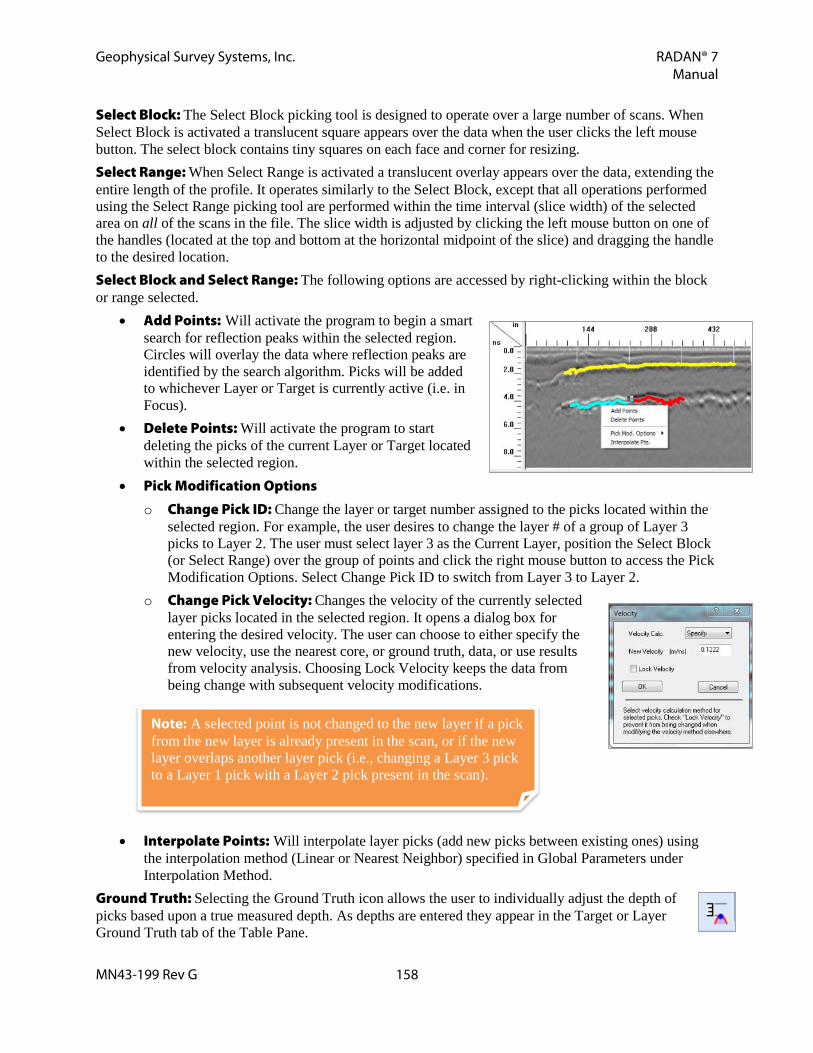
Geophysical Survey Systems, Inc. RADAN® 7 Manual
MN43-199 Rev G 158
Select Block: The Select Block picking tool is designed to operate over a large number of scans. When Select Block is activated a translucent square appears over the data when the user clicks the left mouse button. The select block contains tiny squares on each face and corner for resizing. Select Range: When Select Range is activated a translucent overlay appears over the data, extending the entire length of the profile. It operates similarly to the Select Block, except that all operations performed using the Select Range picking tool are performed within the time interval (slice width) of the selected area on all of the scans in the file. The slice width is adjusted by clicking the left mouse button on one of the handles (located at the top and bottom at the horizontal midpoint of the slice) and dragging the handle to the desired location. Select Block and Select Range: The following options are accessed by right-clicking within the block or range selected.
• Add Points: Will activate the program to begin a smart search for reflection peaks within the selected region. Circles will overlay the data where reflection peaks are identified by the search algorithm. Picks will be added to whichever Layer or Target is currently active (i.e. in Focus).
• Delete Points: Will activate the program to start deleting the picks of the current Layer or Target located within the selected region.
• Pick Modification Options o Change Pick ID: Change the layer or target number assigned to the picks located within the
selected region. For example, the user desires to change the layer # of a group of Layer 3 picks to Layer 2. The user must select layer 3 as the Current Layer, position the Select Block (or Select Range) over the group of points and click the right mouse button to access the Pick Modification Options. Select Change Pick ID to switch from Layer 3 to Layer 2.
o Change Pick Velocity: Changes the velocity of the currently selected layer picks located in the selected region. It opens a dialog box for entering the desired velocity. The user can choose to either specify the new velocity, use the nearest core, or ground truth, data, or use results from velocity analysis. Choosing Lock Velocity keeps the data from being change with subsequent velocity modifications.
• Interpolate Points: Will interpolate layer picks (add new picks between existing ones) using the interpolation method (Linear or Nearest Neighbor) specified in Global Parameters under Interpolation Method.
Ground Truth: Selecting the Ground Truth icon allows the user to individually adjust the depth of picks based upon a true measured depth. As depths are entered they appear in the Target or Layer Ground Truth tab of the Table Pane.
Note: A selected point is not changed to the new layer if a pick from the new layer is already present in the scan, or if the new layer overlaps another layer pick (i.e., changing a Layer 3 pick to a Layer 1 pick with a Layer 2 pick present in the scan).

Geophysical Survey Systems, Inc. RADAN® 7 Manual
MN43-199 Rev G 159
• To enter individual Ground Truth information: o Select Ground Truth from the Interactive Mode window. o Click in the data the spot where the ground truth was collected. o Enter the depth. o Click OK or Cancel.
• To specify all new layer picks to have velocities calculated from the ground truth data, change the Vel. Method from Default Vel. to Core Data in the Layer tab of the Table.
EZ Tracker: Allows the user to add a layer or targets by interpolating data between mouse clicks.
1 Choose Pick Type and choose the appropriate layer or target to Focus (edit).
2 Start: Select to start EZ Tracker. Add layer picks with the left mouse button and delete layer picks with the right mouse button. Picks are interpolated between left mouse button clicks. The closer the click spacing the better the results will be.
3 Right-click to undo the previous selection. This only goes back one time.
4 Stop: Select to stop EZ Tracker.
5 If there are breaks in the layer then select and Stop and Start to skip the break.
Other Options Group Global Parameters
• Single Pt. Search Length: When using Single Point Picking Tool, this setting determines whether the pick is entered at the closest peak or using the cursor length.
• Amplitude Values: Use Data Units, decibels (dB), or Normalized dB. o Data Units: Provides the layer bottom reflection
amplitudes in the actual data values. o dB: Converts the data units amplitudes to decibels
(dB) by using the equation 20*log10(x) where x is the absolute value of the data amplitude. o Normalized dB: Normalizes the data amplitude relative to 32767 for 16 bit data and
2147483648 for 32 bit data before converting to dB. • Interpolation Method: Each time a pick is added a search is performed to locate the
corresponding feature of the reflection that will be used to identify two-way travel time and amplitude. Use either Automatic, Nearest Peak, or Linear. o Automatic: Performs tracking based on a custom algorithm, which is designed to capture
continuous layers that vary with depth. When mouse clicks are spaced more than 20 scans apart this mode switches to Nearest Peak.
o Nearest Peak: Search for the nearest peak between existing picks. o Linear: Draws a straight line between two previously interpreted picks.
• Checking the box will fill the layer with a chosen color in depth pane.

Geophysical Survey Systems, Inc. RADAN® 7 Manual
MN43-199 Rev G 160
• Click OK or Cancel. Help will open a .pdf of the RADAN 7 manual.
Settings
• Load Default Settings: Loads previously saved default settings for Interactive Mode. • Save As Default Settings: Saves the current Interactive Mode settings including all layer
properties and display options. Display Gain To change the Display Gain, click Display Gain in the Home Ribbon or right-click on the data window and select Display Gain. Then select from a preset list of multiples ranging from -6 up to 60. Input a Custom Value by right-clicking and selecting Custom from Display Gain menu. This will change all samples, no matter where they are in the scan trace, by the same amount.
• Altering the display gain does not change data values like Range Gain, which is described later in this section under the Easy Processing and Processing sections.
• Altering the display gain may make it easier to see lower amplitude targets.
Export Group Picks may be exported to a comma delimited ASCII (CSV) file, saved as a JPG image file, or the layer information exported to a KML file (if GPS was collected with the data) for viewing in Google Earth.\ CSV File Click CSV File to export picks to a comma delimited ASCII file and select which fields to export.
• Use Existing: Use existing custom fields that were created in Create Custom or are available for specific applications from GSSI. o Select an Available Export Configuration. o Modify Options for Filtering Data as necessary. o Save the exported CSV file.
• Create Custom: Select fields to export. o Select the desired Export Category. o Choose which Available Fields to include in the CSV
file. o Choose whether to export all of the data or specify
ranges or certain values. If filtering exported data, then modify Options for Filtering Data as necessary.
o Name the custom export. Create a general name for use with other data. o Save the exported CSV File.
Non-Filled Layers Filled Layers

Geophysical Survey Systems, Inc. RADAN® 7 Manual
MN43-199 Rev G 161
• Modify Existing: Modify an existing field list to create a new one. o Select an Available Export Configuration. o Select the desired Export Category. o Choose which Available Fields to include in the CSV file. o Choose whether to export all of the data or specify ranges or certain values. If filtering
exported data, then modify Options for Filtering Data as necessary. o Choose whether to output the data at a specific distance interval. o Save the exported CSV File.
• Use Most Recent: Uses the settings from the last used CSV export. Excel Opens a dialogue box to enter project information. Then create a report in Microsoft Excel with user-entered information, data properties, and an image of the currently selected view. KML File A KML file is a file type used to display geographic data in an earth browser, such as Google Earth and Google Maps. KML files have a tag-based structure with names and attributes used for specific display purposes. RADAN 7 can export certain kinds of information as a KML file and easily view that information in Google Earth. This section discusses exporting layers identified in Interactive Interpretation. In order to create a KML file. The data must have been collected with GPS or GPS coordinates were added to the data.
• GPS Track: Select whether or not to export the GPS trajectory. • User Marks: Select whether or not to export User Marks. • Targets: Select whether or not to export Targets. • Ground Truth: Select whether or not to export Ground Truth
points, or Core Data. • Layers: Selects whether or not to export Layers. Multiple
layers are exported one at a time. o Channel: Selects the data channel to export. Different
channels can be exported if a multi-channel file was collected.
o Output Parameter: Select depth, amplitude, velocity, or time depending on the type of data being exported with the layer.
o Line width: The KML output line width in pixels. o Minimum/Maximum: This sets the range of output values specified in the Output Parameter
option. o Number of Intervals: The number of evenly spaced breakpoints for the output data. o View/Edit Layer Colors: Modify the colors applied to each output interval (based upon
Output Parameter and Number of Intervals previously selected). The output of this is a KML file named after the saved data file and the date of the export. To import into Google Earth, simply drag this file onto Planet Earth and it will zoom to the given location of the data.

Geophysical Survey Systems, Inc. RADAN® 7 Manual
MN43-199 Rev G 162
Google Earth® Ribbon The Google Earth® Ribbon provides viewing and exporting options for data collected with GPS. Options include viewing GPS Tracks, User Marks, Layers, Targets, and Ground Truth in Google Earth, exporting to a KML file, and launching and refreshing Google Earth®.
Display/Save Options Group There are three options in this group for saving or displaying export items in Google Earth®. KML File: Click this button to save selected export items to a KML File. A KML file is a file type used to display geographic data in an earth browser, such as Google Earth® and Google Maps®. KML files have a tag-based structure with names and attributes used for specific display purposes. Google Earth®: Click this button to launch Google Earth® with the selected export options. A Temporary Place will be added to Google Earth®. Google Earth® Refresh: Press this button to refresh Google Earth® with any changes made to the exported items. A new Temporary Place will be added to Google Earth® and will have the same file name as the original file.
Export Items Group This group allows the user to choose which items will be exported as part of a KML file. Only the displayed layers and targets associated with the displayed channel are exported. Layers: Currently displayed layer(s). Select which Layer(s) is displayed by checking the Display box in the Layers Tab of the Table. Targets: Currently displayed target(s). Select which Target(s) is displayed by checking the Display box in the Targets Tab of the Table. User Marks: Export User Marks as they appear in the Way Points Tab of the Table. GPS Path: The GPS Path associated with Channel 1. Ground Truth: Currently displayed Ground Truth data for Layers or Targets.
Layer Options Group This group allows the user to customize how the displayed layers are exported. Output Parameter: There are four Output Parameter options to choose from when exporting layers. Although depth is the typical output parameter, there are applications where other values such as velocity (e.g. new pavement) or amplitude (e.g. bridge deck) provide valuable information.
• Depth
• Amplitude
• Velocity
• Time
Note: Google Earth® must be installed on the user’s computer for either the Google Earth® or the Google Earth® Refresh icons to work.

Geophysical Survey Systems, Inc. RADAN® 7 Manual
MN43-199 Rev G 163
Line Width: Display width of the line in Google Earth®. Number of Intervals: Exported values can be broken into different colors to denote different ranges. The user can specify from 0 to 8 intervals. Minimum Value: The minimum value for the interval range. For example, if the user choses Amplitude for the output parameter, the Minimum Value is the minimum amplitude. Maximum Value: The maximum value for the interval range. For example, if the user choses Amplitude for the output parameter, the Maximum Value is the maximum amplitude. Interval Colors: Opens the Interval Colors dialogue box, which allows the user to select a color for each interval. Click on the down arrows to select a different color or choose Other to open a color editor window.
Settings Group Recall Settings: Press this button to recall the current export settings (Export Items and Layer Options) that have most recently been saved by pressing the Save Settings icon. Save Settings: Press this button to save the current export settings (Export Items and Layer Options) as the default settings for all files.

Geophysical Survey Systems, Inc. RADAN® 7 Manual
MN43-199 Rev G 164
Ground-Coupled BridgeScan This display is designed to process data specifically collected to determine bridge deterioration.
GSSI Button Clicking on the GSSI Button allows the user to:
• Open a File/Project • Assemble Files • Import GPS • Save a File/Project • Save As a File/Project under a different name or
format • Export data • Print data • Close a File/Project • Close All Open Files • Open a previously processed File/Project • Options to change languages • Exit RADAN 7 Software

Geophysical Survey Systems, Inc. RADAN® 7 Manual
MN43-199 Rev G 165
Home Ribbon
File Group Open: Opens the currently selected project folder to open additional files. Save: Saves the selected data file. If multiple files are open it saves the tab that is active. Any new targets or picks added to the data will be saved. Close: Closes the currently selected data file. If multiple files are open it closes the tab that is active.
Data Windows Group LineScan In the linescan display data are displayed in a color-amplitude form, where a color is assigned to a specific positive or negative amplitude value of the recorded signal dependent upon the color table and color transform selected. The vertical scale represents time (or depth) while the horizontal scale represents the horizontal distance traveled by the radar antenna. The Linescan display is the most useful for mapping man-made objects, such as underground storage tanks, pipes, and drums or for mapping geologic layers.
Scope This will display an O-Scope to the right of the linescan data. Hold the left mouse button down while pointing to the linescan data to correspond the same point with the O-Scope using a horizontal line.
3D View This will display the data as a 3D Cube. More information and options on this mode are discussed in the Basic Processing/Tutorials section under Basic 3D Grid Navigation.
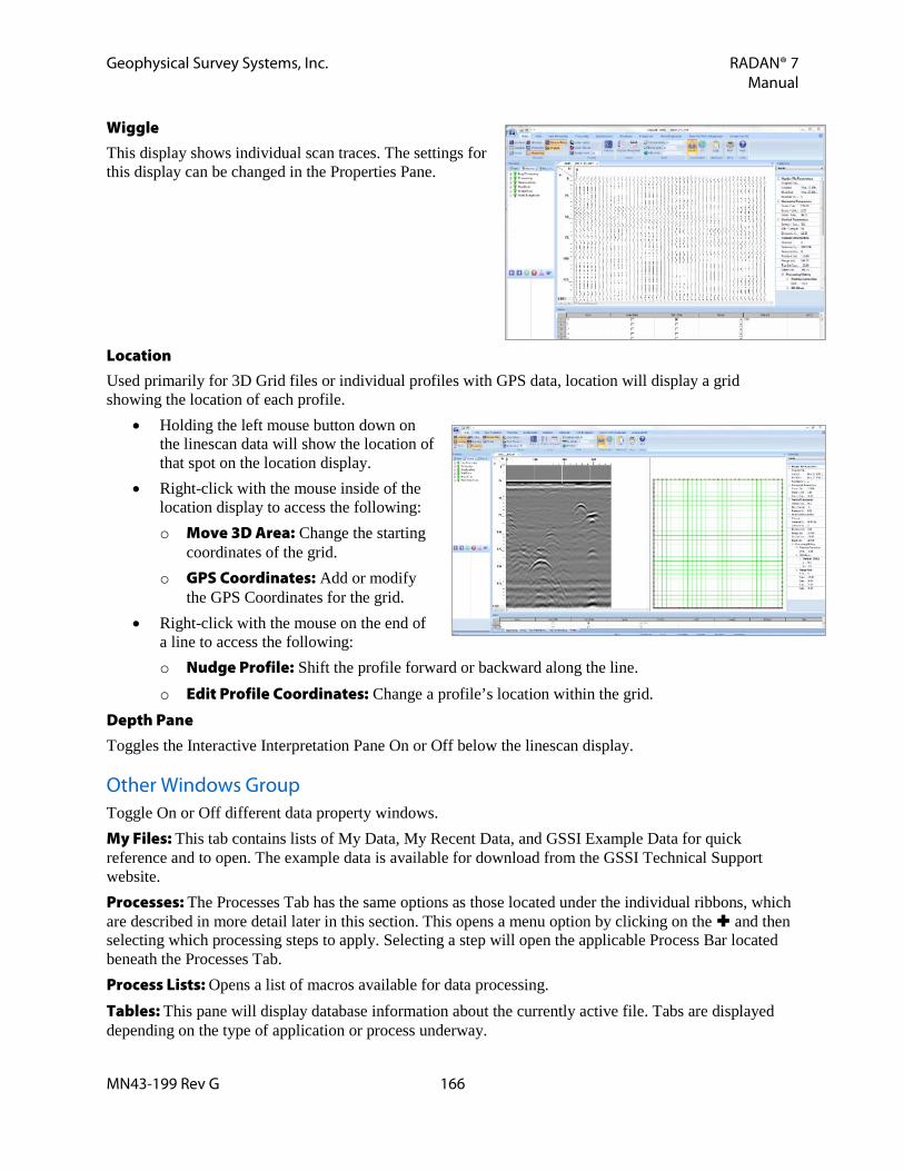
Geophysical Survey Systems, Inc. RADAN® 7 Manual
MN43-199 Rev G 166
Wiggle This display shows individual scan traces. The settings for this display can be changed in the Properties Pane.
Location Used primarily for 3D Grid files or individual profiles with GPS data, location will display a grid showing the location of each profile.
• Holding the left mouse button down on the linescan data will show the location of that spot on the location display.
• Right-click with the mouse inside of the location display to access the following: o Move 3D Area: Change the starting
coordinates of the grid. o GPS Coordinates: Add or modify
the GPS Coordinates for the grid. • Right-click with the mouse on the end of
a line to access the following: o Nudge Profile: Shift the profile forward or backward along the line. o Edit Profile Coordinates: Change a profile’s location within the grid.
Depth Pane Toggles the Interactive Interpretation Pane On or Off below the linescan display.
Other Windows Group Toggle On or Off different data property windows. My Files: This tab contains lists of My Data, My Recent Data, and GSSI Example Data for quick reference and to open. The example data is available for download from the GSSI Technical Support website. Processes: The Processes Tab has the same options as those located under the individual ribbons, which are described in more detail later in this section. This opens a menu option by clicking on the and then selecting which processing steps to apply. Selecting a step will open the applicable Process Bar located beneath the Processes Tab. Process Lists: Opens a list of macros available for data processing. Tables: This pane will display database information about the currently active file. Tabs are displayed depending on the type of application or process underway.

Geophysical Survey Systems, Inc. RADAN® 7 Manual
MN43-199 Rev G 167
File Header: Header information about the displayed file. Window Settings: The Properties Pane automatically updates based on which data display, 2D or 3D is currently selected. Data Channel Properties: Shows channel information for the selected data. Datasets with multiple channels will display individual properties for each channel. Global Settings: Display Global Parameters for all files in a particular project prior to opening any files and allow you to switch between available Application Displays. Once a file is open, the Global Parameters cannot be changed.
Display Group Color Tables Color tables are used to code the amplitude of each scan (i.e., the recorded radar signal). Colors on the left side of the spectrum represent strong negative amplitudes. As the colors go to the right, this represents the amplitude getting weaker (or closer to 0) and the middle of the spectrum is the area of weak amplitude. As the colors go further right from the middle, this represents a stronger positive amplitude.
For example, white in color table 1 corresponds to the highest positive amplitude pulse; therefore, when it appears on the radar record, it means that there is a strong reflection (or a high dielectric contrast).
In some color tables (such as 23), black indicates a low amplitude reflection. Therefore, a large black region on the linescan plot could be indicative of a uniform structure (such as a homogeneous sand deposit) with little or no dielectric contrast.
Color Xforms The Color Transform can be changed to enhance weak amplitude or small contrast reflectors. The color transform determines whether the color scale applied to the radar wave’s amplitude is linear, logarithmic, exponential, or customized. This function can also be used to de-emphasize certain features.
Note: There are 30 different color tables and RADAN defaults to True Grey 17. There are 20 color transforms and
RADAN defaults to Linear Transform 3.
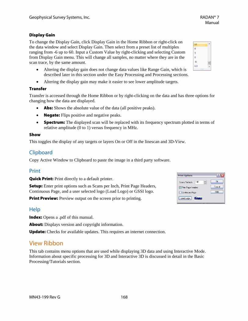
Geophysical Survey Systems, Inc. RADAN® 7 Manual
MN43-199 Rev G 168
Display Gain To change the Display Gain, click Display Gain in the Home Ribbon or right-click on the data window and select Display Gain. Then select from a preset list of multiples ranging from -6 up to 60. Input a Custom Value by right-clicking and selecting Custom from Display Gain menu. This will change all samples, no matter where they are in the scan trace, by the same amount.
• Altering the display gain does not change data values like Range Gain, which is described later in this section under the Easy Processing and Processing sections.
• Altering the display gain may make it easier to see lower amplitude targets. Transfer Transfer is accessed through the Home Ribbon or by right-clicking on the data and has three options for changing how the data are displayed.
• Abs: Shows the absolute value of the data (all positive peaks). • Negate: Flips positive and negative peaks. • Spectrum: The displayed scan will be replaced with its frequency spectrum plotted in terms of
relative amplitude (0 to 1) versus frequency in MHz. Show This toggles the display of any targets or layers On or Off in the linescan and 3D-View.
Clipboard Copy Active Window to Clipboard to paste the image in a third party software.
Print Quick Print: Print directly to a default printer. Setup: Enter print options such as Scans per Inch, Print Page Headers, Continuous Page, and a user selected logo (Load Logo) or GSSI logo. Print Preview: Preview output on the screen prior to printing.
Help Index: Opens a .pdf of this manual. About: Displays version and copyright information. Update: Checks for available updates. This requires an internet connection.
View Ribbon This tab contains menu options that are used while displaying 3D data and using Interactive Mode. Information about specific processing for 3D and Interactive 3D is discussed in detail in the Basic Processing/Tutorials section.

Geophysical Survey Systems, Inc. RADAN® 7 Manual
MN43-199 Rev G 169
Scales Group Vertical Scale: Select between Time (ns), Depth, or Samples. Horizontal Scale: Select between Distance, Coordinates (GPS if available), Scans, or None.
Units Group Select between English or Metric units for the vertical and horizontal scales. Select units for GPS Coordinates.
Coordinates Group Toggle between Local or GPS coordinates display.
Processing Ribbon Create 3D File A step-by-step guide combining collected files, processing the files, and preparing the newly created “bridge” file for further processing. Creation of a 3D file is necessary to complete Bridge Deterioration Mapping, but is not necessary for Bridge QA.
1 Click Create 3D File.
2 Browse to the appropriate folder where the collected bridge files are located.
3 Create an output filename for the newly created bridge 3D file.
4 Click Next.
5 Add the bridge files from the left pane to the right pane by: • Double-clicking on the File, or • Click on the File and click Add > , or • If Appropriate, click Add All, or • Highlight a group of files and click Add > • Remove files from the right pane by doing the same
procedures in the right pane
6 Click Next.

Geophysical Survey Systems, Inc. RADAN® 7 Manual
MN43-199 Rev G 170
7 File Group 3D Area: • Enter the length of the bridge. • Enter the starting distance of the FIRST line collected
from the Curb or Lane Stripe. • Enter the spacing between each profile or line. • Click the down arrow to select how the data were
collected. • Select whether the data were collected Standard or
Inline.
8 Click Next.
9 Adjust File Group Details: Can edit the individual profiles. • Filename: The name of each file collected. • Across Dist.: The distance from the curb of each of the files collected. • Rev. Dir.: If the files were collected in a zig-zag pattern and this was specified, an X will
automatically be entered that the file will need to be reversed. • St. Loc.: This is the starting location of the file • Edit St. Loc.: Correct the starting location of the
file as necessary. • End Loc.: This is the ending location of the file. • Edit End Loc.: Correct the ending location of
the file as necessary.
10 Edit the Starting and Ending Locations of each file follow these steps. • Click Edit St. Loc. or Edit End Loc. for EACH
file, one at a time. • Move the slider bar until the vertical line on the
data matches the beginning of the bridge. This point will likely correspond with the middle of the bridge joint. Use the left and right arrow keys on the keyboard to make minor adjustments, as well as clicking on the up and down arrows on the screen
• Click OK. • Repeat this process for the Starting and Ending Locations for ALL files.

Geophysical Survey Systems, Inc. RADAN® 7 Manual
MN43-199 Rev G 171
11 Click Next.
12 Enter the Bridge Joint Skew Angle: This will be a positive number if the bridge is angled to the right and negative number if the bridge is angled to the left.
13 Click Finish.
Bridge QA This section describes data collection for quality assurance (QA) studies on concrete overlaid bridge decks. This technique is not applicable to asphalt overlaid decks. The goal of this application is to ensure that there is adequate concrete cover over the top layer of reinforcing steel. A single representative profile per travel lane is all that is required to perform Bridge QA. Typically, this profile is along the wheel path of the lane as opposed to the shoulder. The data must be collected perpendicular to the trend of the top layer of rebar. This means that if the rebar are longitudinal, the profiles must be collected across the bridge deck, not along it. If a complete map of cover thickness is required, then a 3D file can be collected following the instructions given in the SIR System manual. Be sure to configure the data collection settings (Gain, Position, Range, Scan and Sample density).
1 When the Bridge QA icon is selected from the Processing Group, the left pane will display the Bridge QA Process Bar.
2 Velocity Calculation: Choose how the radar wave velocity is calculated. • Specify Concrete Velocity: Use this method if Use Calibration Hole Data
is not possible. o Enter the estimated concrete velocity or velocity from previously
processed data. o The default velocity is 3.74 inches/nanosecond (9.5 cm/ns).
• Use Calibration Hole Data (recommended): Calibration data is obtained by measuring the depth to one of the rebar that the antenna passed directly over during data collection. o Enter the calibration hole location relative to the start of the profile line. o Enter the measured rebar depth.
3 Manually Adjustable Parameters: The most common use for the Bridge QA module has been on newly constructed concrete bridge decks containing rebar between 1-4 inches (2.5-10 cm) in depth and at a spacing of 6 inches (15 cm) between rebar. • Minimum Rebar Depth: Closest point to the ground surface where the process will look for
rebar. • Maximum Rebar Depth: Deepest point in the concrete deck where the process will look for
rebar. • Average Spacing between Rebar: Estimated average spacing between rebar.

Geophysical Survey Systems, Inc. RADAN® 7 Manual
MN43-199 Rev G 172
4 Click Apply and Reset, and adjust if necessary.
5 Click OK once desired results are achieved. Deterioration Mapping This technique locates areas of probable concrete deterioration in a bare concrete or asphalt overlaid concrete deck. This is done by graphing the relative reflection amplitudes across the survey area and assigning threshold values to the amplitude range. Areas of deterioration will attenuate (weaken) the radar signal. This process indicates the presence of deterioration and not the type or cause of that deterioration.
1 When the Deterioration Mapping icon is selected from the Processing Group, the left pane will display the Deterioration Mapping Process Bar.
2 Velocity Calculation: Choose how the radar wave velocity is calculated. • Surface: Select the Surface type of the bridge deck. Either Asphalt
Overlay or Concrete Surface. • Time-Zero Amplitude Threshold: RADAN 7 defaults to the location of
the surface. If this isn’t calculated correctly it can manually be adjusted. • Velocity (Top Layer): RADAN 7 will use the velocity from the File Header information. If this
is incorrect it can manually be adjusted. • Dielectric Constant: This is related to the Velocity and will update as the Velocity if modified.
3 Click Apply and Reset, and adjust if necessary.
4 Click OK once desired results are achieved.
2D Interactive Ribbon This ribbon allows you to add targets and layers to your 2D data and display them in 3D.
Interactive Status Group Show: Toggles On or Off the targets and layers already added to the data. Add or Edit: When selected the targets or layers already added to the data will be displayed and you can either edit the existing interpretations or add new ones. Selecting Add or Edit enables the rest of the 2D Interactive Ribbon.
Objects Group Pick Type: Pick between Layer or Target. Focus: In Free Draw mode, this specifies the object that is being entered or modified. If multiple objects have already been drawn they will appear in the drop down menu. New Object: Click here to draw additional objects.

Geophysical Survey Systems, Inc. RADAN® 7 Manual
MN43-199 Rev G 173
Pick Attributes Group Pick Polarity: When picking layers or targets, the user may specify which portion of the reflection to attach new picks to Positive, Negative, Absolute, or None polarity. Search Width: In pixels, enter the search width for the Single Point picking tool.
Pick Tool Group Disabled: Disable Picking Tool. Single Point: Enter Single Points for target picking. A left mouse click adds a point and a right mouse click deletes a point.
• Adding Picks in Single Point Mode o A search will be performed on all of the scans between the left and right inside edges of the
mouse cursor to locate the maximum amplitude. If the search is successful, a pick will appear on the data. The type of search used to locate the new pick can be customized in the Layer Options menu choice (Layer Tab of the Tables Pane).
o A pick will only be successfully added if a reflection can be located over the cursor search width.
o If no pick is added after pressing the left mouse button, reposition the mouse cursor and click the left mouse button again.
o For cases where the reflection peak is reversed polarity, the user would first need to select Neg. Peak for the Layer Properties under Layer Options in the Interactive Interpretation main menu, then place the mouse cursor over a negative polarity reflection.
• Deleting Picks in Single Point Mode: To delete poor picks, a procedure similar to adding picks is followed.
Select Block: The Select Block picking tool is designed to operate over a large number of scans. When Select Block is activated a translucent square appears over the data when the user clicks the left mouse button. The select block contains tiny squares on each face and corner for resizing. Select Range: When Select Range is activated a translucent overlay appears over the data, extending the entire length of the profile. It operates similarly to the Select Block, except that all operations performed using the Select Range picking tool are performed within the time interval (slice width) of the selected area on all of the scans in the file. The slice width is adjusted by clicking the left mouse button on one of the handles (located at the top and bottom at the horizontal midpoint of the slice) and dragging the handle to the desired location. Select Block and Select Range: The following options are accessed by right-clicking within the block or range selected.
• Add Points: Will activate the program to begin a smart search for reflection peaks within the selected region. Circles will overlay the data where reflection peaks are identified by the search algorithm. Picks will be added to whichever Layer or Target is currently active (i.e. in Focus).
• Delete Points: Will activate the program to start deleting the picks of the current Layer or Target located within the selected region.

Geophysical Survey Systems, Inc. RADAN® 7 Manual
MN43-199 Rev G 174
• Pick Modification Options o Change Pick ID: Change the layer or target number assigned to the picks located within the
selected region. For example, the user desires to change the layer # of a group of Layer 3 picks to Layer 2. The user must select layer 3 as the Current Layer, position the Select Block (or Select Range) over the group of points and click the right mouse button to access the Pick Modification Options. Select Change Pick ID to switch from Layer 3 to Layer 2.
o Change Pick Velocity: Changes the velocity of the currently selected layer picks located in the selected region. It opens a dialog box for entering the desired velocity. The user can choose to either specify the new velocity, use the nearest core, or ground truth, data, or use results from velocity analysis. Choosing Lock Velocity keeps the data from being change with subsequent velocity modifications.
• Interpolate Points: Will interpolate layer picks (add new picks between existing ones) using the interpolation method (Linear or Nearest Neighbor) specified in Global Parameters under Interpolation Method.
Ground Truth: Selecting the Ground Truth icon allows the user to individually adjust the depth of picks based upon a true measured depth. As depths are entered they appear in the Target or Layer Ground Truth tab of the Table Pane.
• To enter individual Ground Truth information: o Select Ground Truth from the Interactive Mode window. o Click in the data the spot where the ground truth was collected. o Enter the depth. o Click OK or Cancel.
• To specify all new layer picks to have velocities calculated from the ground truth data, change the Vel. Method from Default Vel. to Core Data in the Layer tab of the Table.
EZ Tracker: Allows the user to add a layer or targets by interpolating data between mouse clicks.
1 Choose Pick Type and choose the appropriate layer or target to Focus (edit).
2 Start: Select to start EZ Tracker. Add layer picks with the left mouse button and delete layer picks with the right mouse button. Picks are interpolated between left mouse button clicks. The closer the click spacing the better the results will be.
3 Right-click to undo the previous selection. This only goes back one time.
4 Stop: Select to stop EZ Tracker.
5 If there are breaks in the layer then select and Stop and Start to skip the break.
Note: A selected point is not changed to the new layer if a pick from the new layer is already present in the scan, or if the new layer overlaps another layer pick (i.e., changing a Layer 3 pick to a Layer 1 pick with a Layer 2 pick present in the scan).

Geophysical Survey Systems, Inc. RADAN® 7 Manual
MN43-199 Rev G 175
Other Options Group Global Parameters
• Single Pt. Search Length: When using Single Point Picking Tool, this setting determines whether the pick is entered at the closest peak or using the cursor length.
• Amplitude Values: Use Data Units, decibels (dB), or Normalized dB. o Data Units: Provides the layer bottom reflection
amplitudes in the actual data values. o dB: Converts the data units amplitudes to decibels
(dB) by using the equation 20*log10(x) where x is the absolute value of the data amplitude. o Normalized dB: Normalizes the data amplitude relative to 32767 for 16 bit data and
2147483648 for 32 bit data before converting to dB. • Interpolation Method: Each time a pick is added a search is performed to locate the
corresponding feature of the reflection that will be used to identify two-way travel time and amplitude. Use either Automatic, Nearest Peak, or Linear. o Automatic: Performs tracking based on a custom algorithm, which is designed to capture
continuous layers that vary with depth. When mouse clicks are spaced more than 20 scans apart this mode switches to Nearest Peak.
o Nearest Peak: Search for the nearest peak between existing picks. o Linear: Draws a straight line between two previously interpreted picks.
• Checking the box will fill the layer with a chosen color in depth pane. • Click OK or Cancel. Help will open a .pdf of the RADAN 7 manual.
Settings
• Load Default Settings: Loads previously saved default settings for Interactive Mode. • Save As Default Settings: Saves the current Interactive Mode settings including all layer
properties and display options.
Non-Filled Layers Filled Layers

Geophysical Survey Systems, Inc. RADAN® 7 Manual
MN43-199 Rev G 176
Display Gain To change the Display Gain, click Display Gain in the Home Ribbon or right-click on the data window and select Display Gain. Then select from a preset list of multiples ranging from -6 up to 60. Input a Custom Value by right-clicking and selecting Custom from Display Gain menu. This will change all samples, no matter where they are in the scan trace, by the same amount.
• Altering the display gain does not change data values like Range Gain, which is described later in this section under the Easy Processing and Processing sections.
• Altering the display gain may make it easier to see lower amplitude targets.
Export Group Picks may be exported to a comma delimited ASCII (CSV) file, saved as a JPG image file, or the layer information exported to a KML file (if GPS was collected with the data) for viewing in Google Earth.\ CSV File Click CSV File to export picks to a comma delimited ASCII file and select which fields to export.
• Use Existing: Use existing custom fields that were created in Create Custom or are available for specific applications from GSSI. o Select an Available Export Configuration. o Modify Options for Filtering Data as necessary. o Save the exported CSV file.
• Create Custom: Select fields to export. o Select the desired Export Category. o Choose which Available Fields to include in the CSV
file. o Choose whether to export all of the data or specify
ranges or certain values. If filtering exported data, then modify Options for Filtering Data as necessary.
o Name the custom export. Create a general name for use with other data.
o Save the exported CSV File. • Modify Existing: Modify an existing field list to create a new one.
o Select an Available Export Configuration. o Select the desired Export Category. o Choose which Available Fields to include in the CSV file. o Choose whether to export all of the data or specify ranges or certain values. If filtering
exported data, then modify Options for Filtering Data as necessary. o Choose whether to output the data at a specific distance interval. o Save the exported CSV File.
• Use Most Recent: Uses the settings from the last used CSV export. Excel Opens a dialogue box to enter project information. Then create a report in Microsoft Excel with user-entered information, data properties, and an image of the currently selected view.

Geophysical Survey Systems, Inc. RADAN® 7 Manual
MN43-199 Rev G 177
KML File A KML file is a file type used to display geographic data in an earth browser, such as Google Earth and Google Maps. KML files have a tag-based structure with names and attributes used for specific display purposes. RADAN 7 can export certain kinds of information as a KML file and easily view that information in Google Earth. This section discusses exporting layers identified in Interactive Interpretation. In order to create a KML file. The data must have been collected with GPS or GPS coordinates were added to the data.
• GPS Track: Select whether or not to export the GPS trajectory.
• User Marks: Select whether or not to export User Marks. • Targets: Select whether or not to export Targets. • Ground Truth: Select whether or not to export Ground
Truth points, or Core Data. • Layers: Selects whether or not to export Layers. Multiple
layers are exported one at a time. o Channel: Selects the data channel to export. Different
channels can be exported if a multi-channel file was collected.
o Output Parameter: Select depth, amplitude, velocity, or time depending on the type of data being exported with the layer.
o Line width: The KML output line width in pixels. o Minimum/Maximum: This sets the range of output
values specified in the Output Parameter option. o Number of Intervals: The number of evenly spaced breakpoints for the output data. o View/Edit Layer Colors: Modify the colors applied to each output interval (based upon
Output Parameter and Number of Intervals previously selected). The output of this is a KML file named after the saved data file and the date of the export. To import into Google Earth, simply drag this file onto Planet Earth and it will zoom to the given location of the data.
Google Earth® Ribbon The Google Earth® Ribbon provides viewing and exporting options for data collected with GPS. Options include viewing GPS Tracks, User Marks, Layers, Targets, and Ground Truth in Google Earth, exporting to a KML file, and launching and refreshing Google Earth®.
Display/Save Options Group There are three options in this group for saving or displaying export items in Google Earth®.

Geophysical Survey Systems, Inc. RADAN® 7 Manual
MN43-199 Rev G 178
KML File: Click this button to save selected export items to a KML File. A KML file is a file type used to display geographic data in an earth browser, such as Google Earth® and Google Maps®. KML files have a tag-based structure with names and attributes used for specific display purposes. Google Earth®: Click this button to launch Google Earth® with the selected export options. A Temporary Place will be added to Google Earth®. Google Earth® Refresh: Press this button to refresh Google Earth® with any changes made to the exported items. A new Temporary Place will be added to Google Earth® and will have the same file name as the original file.
Export Items Group This group allows the user to choose which items will be exported as part of a KML file. Only the displayed layers and targets associated with the displayed channel are exported. Layers: Currently displayed layer(s). Select which Layer(s) is displayed by checking the Display box in the Layers Tab of the Table. Targets: Currently displayed target(s). Select which Target(s) is displayed by checking the Display box in the Targets Tab of the Table. User Marks: Export User Marks as they appear in the Way Points Tab of the Table. GPS Path: The GPS Path associated with Channel 1. Ground Truth: Currently displayed Ground Truth data for Layers or Targets.
Layer Options Group This group allows the user to customize how the displayed layers are exported. Output Parameter: There are four Output Parameter options to choose from when exporting layers. Although depth is the typical output parameter, there are applications where other values such as velocity (e.g. new pavement) or amplitude (e.g. bridge deck) provide valuable information.
• Depth
• Amplitude
• Velocity
• Time
Line Width: Display width of the line in Google Earth®. Number of Intervals: Exported values can be broken into different colors to denote different ranges. The user can specify from 0 to 8 intervals. Minimum Value: The minimum value for the interval range. For example, if the user choses Amplitude for the output parameter, the Minimum Value is the minimum amplitude. Maximum Value: The maximum value for the interval range. For example, if the user choses Amplitude for the output parameter, the Maximum Value is the maximum amplitude.
Note: Google Earth® must be installed on the user’s computer for either the Google Earth® or the Google Earth® Refresh icons to work.

Geophysical Survey Systems, Inc. RADAN® 7 Manual
MN43-199 Rev G 179
Interval Colors: Opens the Interval Colors dialogue box, which allows the user to select a color for each interval. Click on the down arrows to select a different color or choose Other to open a color editor window.
Settings Group Recall Settings: Press this button to recall the current export settings (Export Items and Layer Options) that have most recently been saved by pressing the Save Settings icon. Save Settings: Press this button to save the current export settings (Export Items and Layer Options) as the default settings for all files.

Geophysical Survey Systems, Inc. RADAN® 7 Manual
MN43-199 Rev G 180
Horn BridgeScan The Horn BridgeScan Ribbon is designed to process data specifically collected to determine bridge deterioration using an air-launched horn antenna instead of a ground-coupled antenna.
GSSI Button Clicking on the GSSI Button allows the user to:
• Open a File/Project • Assemble Files • Import GPS • Save a File/Project • Save As a File/Project under a different name or
format • Export data • Print data • Close a File/Project • Close All Open Files • Open a previously processed File/Project • Options to change languages • Exit RADAN 7 Software
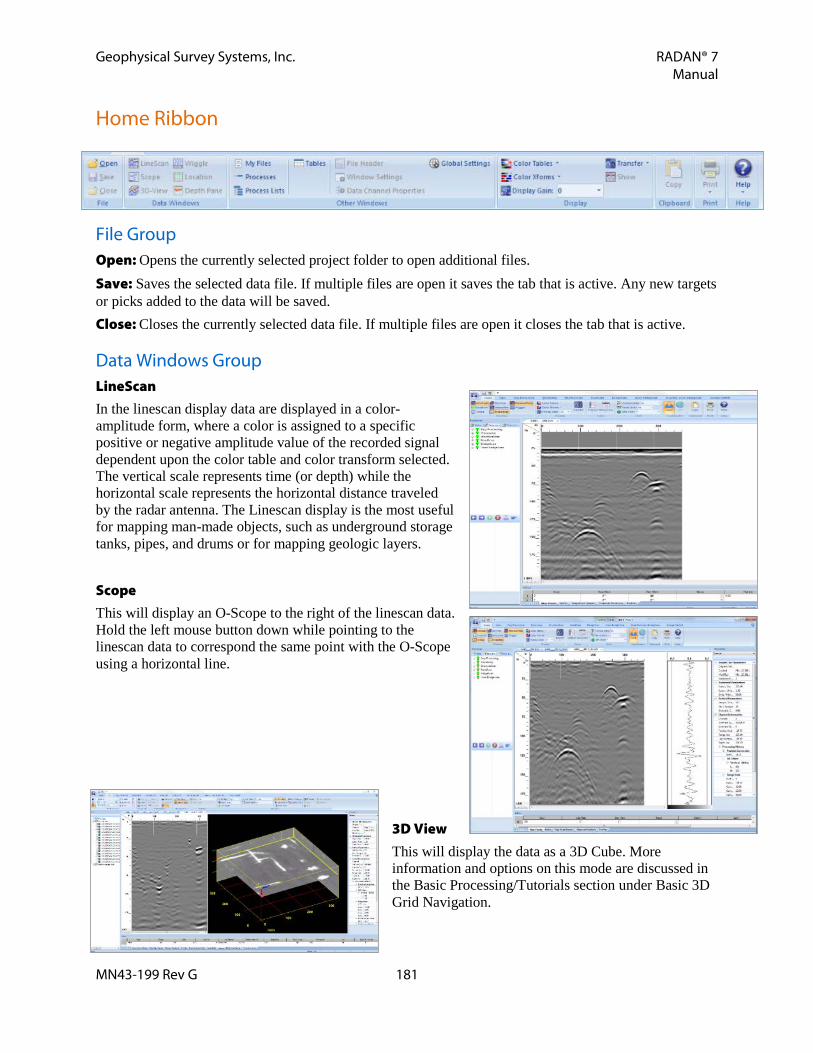
Geophysical Survey Systems, Inc. RADAN® 7 Manual
MN43-199 Rev G 181
Home Ribbon
File Group Open: Opens the currently selected project folder to open additional files. Save: Saves the selected data file. If multiple files are open it saves the tab that is active. Any new targets or picks added to the data will be saved. Close: Closes the currently selected data file. If multiple files are open it closes the tab that is active.
Data Windows Group LineScan In the linescan display data are displayed in a color-amplitude form, where a color is assigned to a specific positive or negative amplitude value of the recorded signal dependent upon the color table and color transform selected. The vertical scale represents time (or depth) while the horizontal scale represents the horizontal distance traveled by the radar antenna. The Linescan display is the most useful for mapping man-made objects, such as underground storage tanks, pipes, and drums or for mapping geologic layers.
Scope This will display an O-Scope to the right of the linescan data. Hold the left mouse button down while pointing to the linescan data to correspond the same point with the O-Scope using a horizontal line.
3D View This will display the data as a 3D Cube. More information and options on this mode are discussed in the Basic Processing/Tutorials section under Basic 3D Grid Navigation.

Geophysical Survey Systems, Inc. RADAN® 7 Manual
MN43-199 Rev G 182
Wiggle This display shows individual scan traces. The settings for this display can be changed in the Properties Pane.
Location Used primarily for 3D Grid files or individual profiles with GPS data, location will display a grid showing the location of each profile.
• Holding the left mouse button down on the linescan data will show the location of that spot on the location display.
• Right-click with the mouse inside of the location display to access the following: o Move 3D Area: Change the starting
coordinates of the grid. o GPS Coordinates: Add or modify the
GPS Coordinates for the grid. • Right-click with the mouse on the end of a
line to access the following: o Nudge Profile: Shift the profile forward
or backward along the line. o Edit Profile Coordinates: Change a profile’s location within the grid.
Depth Pane Toggles the Interactive Interpretation Pane On or Off below the linescan display.
Other Windows Group Toggle On or Off different data property windows. My Files: This tab contains lists of My Data, My Recent Data, and GSSI Example Data for quick reference and to open. The example data is available for download from the GSSI Technical Support website. Processes: The Processes Tab has the same options as those located under the individual ribbons, which are described in more detail later in this section. This opens a menu option by clicking on the and then selecting which processing steps to apply. Selecting a step will open the applicable Process Bar located beneath the Processes Tab. Process Lists: Opens a list of macros available for data processing. Tables: This pane will display database information about the currently active file. Tabs are displayed depending on the type of application or process underway. File Header: Header information about the displayed file.

Geophysical Survey Systems, Inc. RADAN® 7 Manual
MN43-199 Rev G 183
Window Settings: The Properties Pane automatically updates based on which data display, 2D or 3D is currently selected. Data Channel Properties: Shows channel information for the selected data. Datasets with multiple channels will display individual properties for each channel. Global Settings: Display Global Parameters for all files in a particular project prior to opening any files and allow you to switch between available Application Displays. Once a file is open, the Global Parameters cannot be changed.
Display Group Color Tables Color tables are used to code the amplitude of each scan (i.e., the recorded radar signal). Colors on the left side of the spectrum represent strong negative amplitudes. As the colors go to the right, this represents the amplitude getting weaker (or closer to 0) and the middle of the spectrum is the area of weak amplitude. As the colors go further right from the middle, this represents a stronger positive amplitude.
• For example, white in color table 1 corresponds to the highest positive amplitude pulse; therefore, when it appears on the radar record, it means that there is a strong reflection (or a high dielectric contrast).
• In some color tables (such as 23), black indicates a low amplitude reflection. Therefore, a large black region on the linescan plot could be indicative of a uniform structure (such as a homogeneous sand deposit) with little or no dielectric contrast.
Color Xforms The Color Transform can be changed to enhance weak amplitude or small contrast reflectors. The color transform determines whether the color scale applied to the radar wave’s amplitude is linear, logarithmic, exponential, or customized. This function can also be used to de-emphasize certain features.
Display Gain To change the Display Gain, click Display Gain in the Home Ribbon or right-click on the data window and select Display Gain. Then select from a preset list of multiples ranging from -6 up to 60. Input a Custom Value by right-clicking and selecting Custom from Display Gain menu. This will change all samples, no matter where they are in the scan trace, by the same amount.
• Altering the display gain does not change data values like Range Gain, which is described later in this section under the Easy Processing and Processing sections.
• Altering the display gain may make it easier to see lower amplitude targets.
Note: There are 30 different color tables and RADAN defaults to True Grey 17. There are 20 color transforms and RADAN defaults to Linear Transform 3.
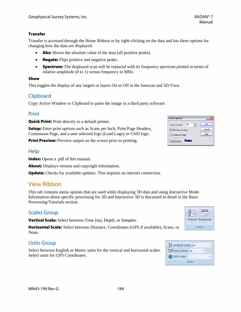
Geophysical Survey Systems, Inc. RADAN® 7 Manual
MN43-199 Rev G 184
Transfer Transfer is accessed through the Home Ribbon or by right-clicking on the data and has three options for changing how the data are displayed.
• Abs: Shows the absolute value of the data (all positive peaks). • Negate: Flips positive and negative peaks. • Spectrum: The displayed scan will be replaced with its frequency spectrum plotted in terms of
relative amplitude (0 to 1) versus frequency in MHz. Show This toggles the display of any targets or layers On or Off in the linescan and 3D-View.
Clipboard Copy Active Window to Clipboard to paste the image in a third party software.
Print Quick Print: Print directly to a default printer. Setup: Enter print options such as Scans per Inch, Print Page Headers, Continuous Page, and a user selected logo (Load Logo) or GSSI logo. Print Preview: Preview output on the screen prior to printing.
Help Index: Opens a .pdf of this manual. About: Displays version and copyright information. Update: Checks for available updates. This requires an internet connection.
View Ribbon This tab contains menu options that are used while displaying 3D data and using Interactive Mode. Information about specific processing for 3D and Interactive 3D is discussed in detail in the Basic Processing/Tutorials section.
Scales Group Vertical Scale: Select between Time (ns), Depth, or Samples. Horizontal Scale: Select between Distance, Coordinates (GPS if available), Scans, or None.
Units Group Select between English or Metric units for the vertical and horizontal scales. Select units for GPS Coordinates.

Geophysical Survey Systems, Inc. RADAN® 7 Manual
MN43-199 Rev G 185
Coordinates Group Toggle between Local or GPS coordinates display.
Processing Ribbon
Create 3D File A step-by-step guide combining collected files, processing the files, and preparing the newly created “bridge” file for further processing. Creation of a 3D file is necessary to complete Bridge Deterioration Mapping, but is not necessary for Bridge QA.
1 Click Create 3D File.
2 Browse to the appropriate folder where the collected bridge files are located.
3 Create an output filename for the newly created bridge 3D file.
4 Click Next.
5 Add the bridge files from the left pane to the right pane by: • Double-clicking on the File, or • Click on the File and click Add > , or • If Appropriate, click Add All, or • Highlight a group of files and click Add > • Remove files from the right pane by doing the same
procedures in the right pane
6 Click Next.
7 File Group 3D Area: • Enter the length of the bridge. • Enter the starting distance of the FIRST line
collected from the Curb or Lane Stripe. • Enter the spacing between each profile or line. • Click the down arrow to select how the data were
collected. • Select whether the data were collected Standard or
Inline.
8 Click Next.
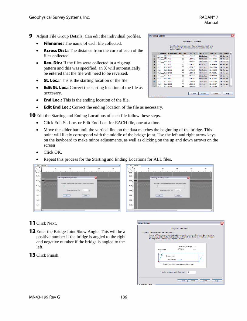
Geophysical Survey Systems, Inc. RADAN® 7 Manual
MN43-199 Rev G 186
9 Adjust File Group Details: Can edit the individual profiles. • Filename: The name of each file collected. • Across Dist.: The distance from the curb of each of the
files collected. • Rev. Dir.: If the files were collected in a zig-zag
pattern and this was specified, an X will automatically be entered that the file will need to be reversed.
• St. Loc.: This is the starting location of the file • Edit St. Loc.: Correct the starting location of the file as
necessary. • End Loc.: This is the ending location of the file. • Edit End Loc.: Correct the ending location of the file as necessary.
10 Edit the Starting and Ending Locations of each file follow these steps. • Click Edit St. Loc. or Edit End Loc. for EACH file, one at a time. • Move the slider bar until the vertical line on the data matches the beginning of the bridge. This
point will likely correspond with the middle of the bridge joint. Use the left and right arrow keys on the keyboard to make minor adjustments, as well as clicking on the up and down arrows on the screen
• Click OK. • Repeat this process for the Starting and Ending Locations for ALL files.
11 Click Next.
12 Enter the Bridge Joint Skew Angle: This will be a positive number if the bridge is angled to the right and negative number if the bridge is angled to the left.
13 Click Finish.

Geophysical Survey Systems, Inc. RADAN® 7 Manual
MN43-199 Rev G 187
Processing Group Reflection Picking Reflection Picking corrects the ground surface of RoadScan data based on the previously created Horn Calibration .CZT file. This process eliminates unwanted signal noise to enhance reflections from the pavement layers making them easier to track. Measures the return times of the reflections and calculates the two-way travel time for each of the pavement layers from the data.
1 When the Reflection Picking icon is selected from the Processing Group, the left pane will display the Reflection Picking Process Bar.
2 Cal(ibration) File Select Method: Select the method for identifying the .CZT, calibration file. • User Select: Manually choose the calibration file. • Current Output Folder: Will search for a .CZT file in the current Output Directory specified in
Global Parameters under the Properties Pane prior to opening any data. • Antenna Database: If there is a serial number and model number an antenna database will
automatically be created. If survey conditions are consistent enough the user does have to recollect a calibration file prior to each survey. Instead the antenna database can be used.
• Auto Select: If Auto Save is set to No it will search the current Output Directory specified in Global Parameters. If the Auto Save is set to Yes it will look in the Proc folder that is automatically created within the Source Directory as specified in Global Parameters. If more than one .CZT is located in the specified folder, RADAN 7 will select the first one in alphanumeric order. If no .CZT file is found it will search the antenna database.
3 Automatic Mode: Select whether or not to use standard settings. If No is selected the following options are available. • Background Removal: Removes horizontal banding in the data. • Starting Depth: Specifies the starting depth for Background Removal. • Apply Inline Position Correction: Correct for inline offset specified in Channel Positions tab
of the Table Pane.
4 Click Apply and Reset, and adjust if necessary.
5 Click OK once desired settings are achieved. RADAN 7 will prompt the user to specify an antenna calibration file.
Horn Bridge Analysis This technique locates areas of probable concrete deterioration in a bare concrete or asphalt overlaid concrete deck. This is done by graphing the relative reflection amplitudes across the survey area and assigning threshold values to the amplitude range. Areas of deterioration will attenuate (weaken) the radar signal. This process indicates the presence of deterioration and not the type or cause of that deterioration.

Geophysical Survey Systems, Inc. RADAN® 7 Manual
MN43-199 Rev G 188
1 When the Deterioration Mapping icon is selected from the Processing Group, the left pane will display the Deterioration Mapping Process Bar.
2 Velocity Calculation: Choose how the radar wave velocity is calculated. • Surface: Select the Surface type of the bridge deck. Either Asphalt Overlay
or Concrete Surface. • Time-Zero Amplitude Threshold: RADAN 7 defaults to the location of the
surface. If this isn’t calculated correctly it can manually be adjusted. • Velocity (Top Layer): RADAN 7 will use the velocity from the File Header information. If this is
incorrect it can manually be adjusted. • Dielectric Constant: This is related to the Velocity and will update as the Velocity if modified.
3 Click Apply and Reset, and adjust if necessary.
4 Click OK once desired results are achieved.
Preset Lists Group Asphalt and Concrete: Choosing either Asphalt or Concrete will automatically run a set group of processes (macros). This allows the user to quickly apply more commonly used settings for data collected over roads a Concrete Surface or those with an Asphalt Overlay.
2D Interactive Ribbon
This ribbon allows you to add targets and layers to your 2D data and display them in 3D.
Interactive Status Group Show: Toggles On or Off the targets and layers already added to the data. Add or Edit: When selected the targets or layers already added to the data will be displayed and you can either edit the existing interpretations or add new ones. Selecting Add or Edit enables the rest of the 2D Interactive Ribbon.
Objects Group Pick Type: Pick between Layer or Target. Focus: In Free Draw mode, this specifies the object that is being entered or modified. If multiple objects have already been drawn they will appear in the drop down menu. New Object: Click here to draw additional objects.
Pick Attributes Group Pick Polarity: When picking layers or targets, the user may specify which portion of the reflection to attach new picks to Positive, Negative, Absolute, or None polarity. Search Width: In pixels, enter the search width for the Single Point picking tool.
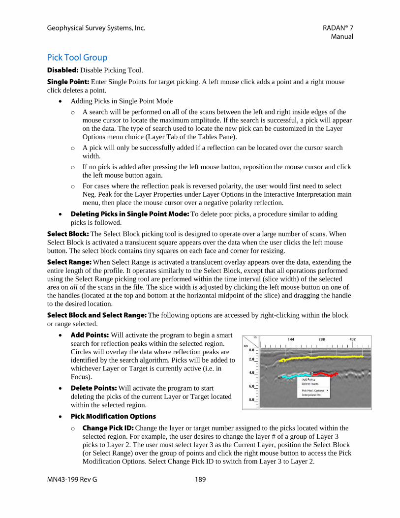
Geophysical Survey Systems, Inc. RADAN® 7 Manual
MN43-199 Rev G 189
Pick Tool Group Disabled: Disable Picking Tool. Single Point: Enter Single Points for target picking. A left mouse click adds a point and a right mouse click deletes a point.
• Adding Picks in Single Point Mode o A search will be performed on all of the scans between the left and right inside edges of the
mouse cursor to locate the maximum amplitude. If the search is successful, a pick will appear on the data. The type of search used to locate the new pick can be customized in the Layer Options menu choice (Layer Tab of the Tables Pane).
o A pick will only be successfully added if a reflection can be located over the cursor search width.
o If no pick is added after pressing the left mouse button, reposition the mouse cursor and click the left mouse button again.
o For cases where the reflection peak is reversed polarity, the user would first need to select Neg. Peak for the Layer Properties under Layer Options in the Interactive Interpretation main menu, then place the mouse cursor over a negative polarity reflection.
• Deleting Picks in Single Point Mode: To delete poor picks, a procedure similar to adding picks is followed.
Select Block: The Select Block picking tool is designed to operate over a large number of scans. When Select Block is activated a translucent square appears over the data when the user clicks the left mouse button. The select block contains tiny squares on each face and corner for resizing. Select Range: When Select Range is activated a translucent overlay appears over the data, extending the entire length of the profile. It operates similarly to the Select Block, except that all operations performed using the Select Range picking tool are performed within the time interval (slice width) of the selected area on all of the scans in the file. The slice width is adjusted by clicking the left mouse button on one of the handles (located at the top and bottom at the horizontal midpoint of the slice) and dragging the handle to the desired location. Select Block and Select Range: The following options are accessed by right-clicking within the block or range selected.
• Add Points: Will activate the program to begin a smart search for reflection peaks within the selected region. Circles will overlay the data where reflection peaks are identified by the search algorithm. Picks will be added to whichever Layer or Target is currently active (i.e. in Focus).
• Delete Points: Will activate the program to start deleting the picks of the current Layer or Target located within the selected region.
• Pick Modification Options o Change Pick ID: Change the layer or target number assigned to the picks located within the
selected region. For example, the user desires to change the layer # of a group of Layer 3 picks to Layer 2. The user must select layer 3 as the Current Layer, position the Select Block (or Select Range) over the group of points and click the right mouse button to access the Pick Modification Options. Select Change Pick ID to switch from Layer 3 to Layer 2.

Geophysical Survey Systems, Inc. RADAN® 7 Manual
MN43-199 Rev G 190
o Change Pick Velocity: Changes the velocity of the currently selected layer picks located in the selected region. It opens a dialog box for entering the desired velocity. The user can choose to either specify the new velocity, use the nearest core, or ground truth, data, or use results from velocity analysis. Choosing Lock Velocity keeps the data from being change with subsequent velocity modifications.
• Interpolate Points: Will interpolate layer picks (add new picks between existing ones) using the interpolation method (Linear or Nearest Neighbor) specified in Global Parameters under Interpolation Method.
Ground Truth: Selecting the Ground Truth icon allows the user to individually adjust the depth of picks based upon a true measured depth. As depths are entered they appear in the Target or Layer Ground Truth tab of the Table Pane.
• To enter individual Ground Truth information: o Select Ground Truth from the Interactive Mode window. o Click in the data the spot where the ground truth was collected. o Enter the depth. o Click OK or Cancel.
• To specify all new layer picks to have velocities calculated from the ground truth data, change the Vel. Method from Default Vel. to Core Data in the Layer tab of the Table.
EZ Tracker: Allows the user to add a layer or targets by interpolating data between mouse clicks.
1 Choose Pick Type and choose the appropriate layer or target to Focus (edit).
2 Start: Select to start EZ Tracker. Add layer picks with the left mouse button and delete layer picks with the right mouse button. Picks are interpolated between left mouse button clicks. The closer the click spacing the better the results will be.
3 Right-click to undo the previous selection. This only goes back one time.
4 Stop: Select to stop EZ Tracker.
5 If there are breaks in the layer then select and Stop and Start to skip the break.
Note: A selected point is not changed to the new layer if a pick from the new layer is already present in the scan, or if the new layer overlaps another layer pick (i.e., changing a Layer 3 pick to a Layer 1 pick with a Layer 2 pick present in the scan).

Geophysical Survey Systems, Inc. RADAN® 7 Manual
MN43-199 Rev G 191
Other Options Group Global Parameters
• Single Pt. Search Length: When using Single Point Picking Tool, this setting determines whether the pick is entered at the closest peak or using the cursor length.
• Amplitude Values: Use Data Units, decibels (dB), or Normalized dB. o Data Units: Provides the layer bottom reflection
amplitudes in the actual data values. o dB: Converts the data units amplitudes to decibels (dB) by using the equation 20*log10(x)
where x is the absolute value of the data amplitude. o Normalized dB: Normalizes the data amplitude relative to 32767 for 16 bit data and
2147483648 for 32 bit data before converting to dB. • Interpolation Method: Each time a pick is added a search is performed to locate the
corresponding feature of the reflection that will be used to identify two-way travel time and amplitude. Use either Automatic, Nearest Peak, or Linear. o Automatic: Performs tracking based on a custom algorithm, which is designed to capture
continuous layers that vary with depth. When mouse clicks are spaced more than 20 scans apart this mode switches to Nearest Peak.
o Nearest Peak: Search for the nearest peak between existing picks. o Linear: Draws a straight line between two previously interpreted picks.
• Checking the box will fill the layer with a chosen color in depth pane. • Click OK or Cancel. Help will open a .pdf of the RADAN 7 manual.
Settings
• Load Default Settings: Loads previously saved default settings for Interactive Mode. • Save As Default Settings: Saves the current Interactive Mode settings including all layer
properties and display options.
Non-Filled Layers Filled Layers

Geophysical Survey Systems, Inc. RADAN® 7 Manual
MN43-199 Rev G 192
Display Gain To change the Display Gain, click Display Gain in the Home Ribbon or right-click on the data window and select Display Gain. Then select from a preset list of multiples ranging from -6 up to 60. Input a Custom Value by right-clicking and selecting Custom from Display Gain menu. This will change all samples, no matter where they are in the scan trace, by the same amount.
• Altering the display gain does not change data values like Range Gain, which is described later in this section under the Easy Processing and Processing sections.
• Altering the display gain may make it easier to see lower amplitude targets.
Export Group Picks may be exported to a comma delimited ASCII (CSV) file, saved as a JPG image file, or the layer information exported to a KML file (if GPS was collected with the data) for viewing in Google Earth.\ CSV File Click CSV File to export picks to a comma delimited ASCII file and select which fields to export.
• Use Existing: Use existing custom fields that were created in Create Custom or are available for specific applications from GSSI. o Select an Available Export Configuration. o Modify Options for Filtering Data as necessary. o Save the exported CSV file.
• Create Custom: Select fields to export. o Select the desired Export Category. o Choose which Available Fields to include in the CSV
file. o Choose whether to export all of the data or specify
ranges or certain values. If filtering exported data, then modify Options for Filtering Data as necessary.
o Name the custom export. Create a general name for use with other data.
o Save the exported CSV File. • Modify Existing: Modify an existing field list to create a new one.
o Select an Available Export Configuration. o Select the desired Export Category. o Choose which Available Fields to include in the CSV file. o Choose whether to export all of the data or specify ranges or certain values. If filtering
exported data, then modify Options for Filtering Data as necessary. o Choose whether to output the data at a specific distance interval. o Save the exported CSV File.
• Use Most Recent: Uses the settings from the last used CSV export. Excel Opens a dialogue box to enter project information. Then create a report in Microsoft Excel with user-entered information, data properties, and an image of the currently selected view.

Geophysical Survey Systems, Inc. RADAN® 7 Manual
MN43-199 Rev G 193
KML File A KML file is a file type used to display geographic data in an earth browser, such as Google Earth and Google Maps. KML files have a tag-based structure with names and attributes used for specific display purposes. RADAN 7 can export certain kinds of information as a KML file and easily view that information in Google Earth. This section discusses exporting layers identified in Interactive Interpretation. In order to create a KML file. The data must have been collected with GPS or GPS coordinates were added to the data.
• GPS Track: Select whether or not to export the GPS trajectory. • User Marks: Select whether or not to export User Marks. • Targets: Select whether or not to export Targets. • Ground Truth: Select whether or not to export Ground Truth
points, or Core Data. • Layers: Selects whether or not to export Layers. Multiple layers
are exported one at a time. o Channel: Selects the data channel to export. Different
channels can be exported if a multi-channel file was collected. o Output Parameter: Select depth, amplitude, velocity, or time depending on the type of data
being exported with the layer. o Line width: The KML output line width in pixels. o Minimum/Maximum: This sets the range of output values specified in the Output Parameter
option. o Number of Intervals: The number of evenly spaced breakpoints for the output data. o View/Edit Layer Colors: Modify the colors applied to each output interval (based upon
Output Parameter and Number of Intervals previously selected). The output of this is a KML file named after the saved data file and the date of the export. To import into Google Earth, simply drag this file onto Planet Earth and it will zoom to the given location of the data.
Google Earth® Ribbon The Google Earth® Ribbon provides viewing and exporting options for data collected with GPS. Options include viewing GPS Tracks, User Marks, Layers, Targets, and Ground Truth in Google Earth, exporting to a KML file, and launching and refreshing Google Earth®.
Display/Save Options Group There are three options in this group for saving or displaying export items in Google Earth®. KML File: Click this button to save selected export items to a KML File. A KML file is a file type used to display geographic data in an earth browser, such as Google Earth® and Google Maps®. KML files have a tag-based structure with names and attributes used for specific display purposes.

Geophysical Survey Systems, Inc. RADAN® 7 Manual
MN43-199 Rev G 194
Google Earth®: Click this button to launch Google Earth® with the selected export options. A Temporary Place will be added to Google Earth®. Google Earth® Refresh: Press this button to refresh Google Earth® with any changes made to the exported items. A new Temporary Place will be added to Google Earth® and will have the same file name as the original file.
Export Items Group This group allows the user to choose which items will be exported as part of a KML file. Only the displayed layers and targets associated with the displayed channel are exported. Layers: Currently displayed layer(s). Select which Layer(s) is displayed by checking the Display box in the Layers Tab of the Table. Targets: Currently displayed target(s). Select which Target(s) is displayed by checking the Display box in the Targets Tab of the Table. User Marks: Export User Marks as they appear in the Way Points Tab of the Table. GPS Path: The GPS Path associated with Channel 1. Ground Truth: Currently displayed Ground Truth data for Layers or Targets.
Layer Options Group This group allows the user to customize how the displayed layers are exported. Output Parameter: There are four Output Parameter options to choose from when exporting layers. Although depth is the typical output parameter, there are applications where other values such as velocity (e.g. new pavement) or amplitude (e.g. bridge deck) provide valuable information.
• Depth
• Amplitude
• Velocity
• Time
Line Width: Display width of the line in Google Earth®. Number of Intervals: Exported values can be broken into different colors to denote different ranges. The user can specify from 0 to 8 intervals. Minimum Value: The minimum value for the interval range. For example, if the user choses Amplitude for the output parameter, the Minimum Value is the minimum amplitude. Maximum Value: The maximum value for the interval range. For example, if the user choses Amplitude for the output parameter, the Maximum Value is the maximum amplitude. Interval Colors: Opens the Interval Colors dialogue box, which allows the user to select a color for each interval. Click on the down arrows to select a different color or choose Other to open a color editor window.
Note: Google Earth® must be installed on the user’s computer for either the Google Earth® or the Google Earth® Refresh icons to work.

Geophysical Survey Systems, Inc. RADAN® 7 Manual
MN43-199 Rev G 195
Settings Group Recall Settings: Press this button to recall the current export settings (Export Items and Layer Options) that have most recently been saved by pressing the Save Settings icon. Save Settings: Press this button to save the current export settings (Export Items and Layer Options) as the default settings for all files.

Geophysical Survey Systems, Inc. RADAN® 7 Manual
MN43-199 Rev G 196
Dual Polarization Horn BridgeScan The Dual Polarity Horn BridgeScan Ribbon is designed to process data specifically collected to determine bridge deterioration using three air-launched horn antennas instead of a ground-coupled antenna. The antennas are configured with two 1 GHz horn antennas positioned inline (one behind the other) and one antenna oriented at 90 degrees relative to the other antenna so that the radiated polarization is perpendicular. During data processing the data from one antenna is subtracted from the other antenna to isolate the reflection from the top rebar in the bridge deck. For asphalt-overlaid bridge decks the concrete surface reflection interferes in time with the top rebar reflections. The concrete surface reflection from both antennas is approximately the same, but one antenna orientation is more sensitive to the top rebar. Subtracting the data from the two antennas enhances the top rebar reflection.

Geophysical Survey Systems, Inc. RADAN® 7 Manual
MN43-199 Rev G 197
GSSI Button Clicking on the GSSI Button allows the user to:
• Open a File/Project • Assemble Files • Import GPS • Save a File/Project • Save As a File/Project under a different name or
format • Export data • Print data • Close a File/Project • Close All Open Files • Open a previously processed File/Project • Options to change languages • Exit RADAN 7 Software
Home Ribbon
File Group Open: Opens the currently selected project folder to open additional files. Save: Saves the selected data file. If multiple files are open it saves the tab that is active. Any new targets or picks added to the data will be saved. Close: Closes the currently selected data file. If multiple files are open it closes the tab that is active.
Data Windows Group LineScan In the linescan display data are displayed in a color-amplitude form, where a color is assigned to a specific positive or negative amplitude value of the recorded signal dependent upon the color table and color transform selected. The vertical scale represents time (or depth) while the horizontal scale represents the horizontal distance traveled by the radar antenna. The Linescan display is the most useful for mapping man-made objects, such as underground storage tanks, pipes, and drums or for mapping geologic layers.

Geophysical Survey Systems, Inc. RADAN® 7 Manual
MN43-199 Rev G 198
Scope This will display an O-Scope to the right of the linescan data. Hold the left mouse button down while pointing to the linescan data to correspond the same point with the O-Scope using a horizontal line.
3D View This will display the data as a 3D Cube. More information and options on this mode are discussed in the Basic Processing/Tutorials section under Basic 3D Grid Navigation.
Wiggle This display shows individual scan traces. The settings for this display can be changed in the Properties Pane. Location Used primarily for 3D Grid files or individual profiles with GPS data, location will display a grid showing the location of each profile.
• Holding the left mouse button down on the linescan data will show the location of that spot on the location display.
• Right-click with the mouse inside of the location display to access the following: o Move 3D Area: Change the starting
coordinates of the grid. o GPS Coordinates: Add or modify
the GPS Coordinates for the grid. • Right-click with the mouse on the end of a line to access the following:
o Nudge Profile: Shift the profile forward or backward along the line. o Edit Profile Coordinates: Change a profile’s location within the grid.
Depth Pane Toggles the Interactive Interpretation Pane On or Off below the linescan display.
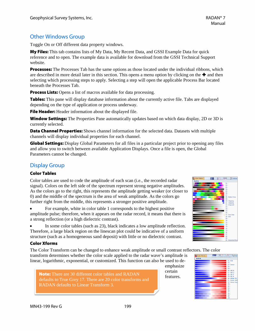
Geophysical Survey Systems, Inc. RADAN® 7 Manual
MN43-199 Rev G 199
Other Windows Group Toggle On or Off different data property windows. My Files: This tab contains lists of My Data, My Recent Data, and GSSI Example Data for quick reference and to open. The example data is available for download from the GSSI Technical Support website. Processes: The Processes Tab has the same options as those located under the individual ribbons, which are described in more detail later in this section. This opens a menu option by clicking on the and then selecting which processing steps to apply. Selecting a step will open the applicable Process Bar located beneath the Processes Tab. Process Lists: Opens a list of macros available for data processing. Tables: This pane will display database information about the currently active file. Tabs are displayed depending on the type of application or process underway. File Header: Header information about the displayed file. Window Settings: The Properties Pane automatically updates based on which data display, 2D or 3D is currently selected. Data Channel Properties: Shows channel information for the selected data. Datasets with multiple channels will display individual properties for each channel. Global Settings: Display Global Parameters for all files in a particular project prior to opening any files and allow you to switch between available Application Displays. Once a file is open, the Global Parameters cannot be changed.
Display Group Color Tables Color tables are used to code the amplitude of each scan (i.e., the recorded radar signal). Colors on the left side of the spectrum represent strong negative amplitudes. As the colors go to the right, this represents the amplitude getting weaker (or closer to 0) and the middle of the spectrum is the area of weak amplitude. As the colors go further right from the middle, this represents a stronger positive amplitude. • For example, white in color table 1 corresponds to the highest positive amplitude pulse; therefore, when it appears on the radar record, it means that there is a strong reflection (or a high dielectric contrast). • In some color tables (such as 23), black indicates a low amplitude reflection. Therefore, a large black region on the linescan plot could be indicative of a uniform structure (such as a homogeneous sand deposit) with little or no dielectric contrast. Color Xforms The Color Transform can be changed to enhance weak amplitude or small contrast reflectors. The color transform determines whether the color scale applied to the radar wave’s amplitude is linear, logarithmic, exponential, or customized. This function can also be used to de-
emphasize certain features.
Note: There are 30 different color tables and RADAN defaults to True Grey 17. There are 20 color transforms and RADAN defaults to Linear Transform 3.

Geophysical Survey Systems, Inc. RADAN® 7 Manual
MN43-199 Rev G 200
Display Gain To change the Display Gain, click Display Gain in the Home Ribbon or right-click on the data window and select Display Gain. Then select from a preset list of multiples ranging from -6 up to 60. Input a Custom Value by right-clicking and selecting Custom from Display Gain menu. This will change all samples, no matter where they are in the scan trace, by the same amount.
• Altering the display gain does not change data values like Range Gain, which is described later in this section under the Easy Processing and Processing sections.
• Altering the display gain may make it easier to see lower amplitude targets. Transfer Transfer is accessed through the Home Ribbon or by right-clicking on the data and has three options for changing how the data are displayed.
Abs: Shows the absolute value of the data (all positive peaks). Negate: Flips positive and negative peaks. Spectrum: The displayed scan will be replaced with its frequency spectrum plotted in terms of
relative amplitude (0 to 1) versus frequency in MHz. Show This toggles the display of any targets or layers On or Off in the linescan and 3D-View.
Clipboard Copy Active Window to Clipboard to paste the image in a third party software.
Print Quick Print: Print directly to a default printer. Setup: Enter print options such as Scans per Inch, Print Page Headers, Continuous Page, and a user selected logo (Load Logo) or GSSI logo. Print Preview: Preview output on the screen prior to printing.
Help Index: Opens a .pdf of this manual. About: Displays version and copyright information. Update: Checks for available updates. This requires an internet connection.
View Ribbon This tab contains menu options that are used while displaying 3D data and using Interactive Mode. Information about specific processing for 3D and Interactive 3D is discussed in detail in the Basic Processing/Tutorials section.

Geophysical Survey Systems, Inc. RADAN® 7 Manual
MN43-199 Rev G 201
Scales Group Vertical Scale: Select between Time (ns), Depth, or Samples. Horizontal Scale: Select between Distance, Coordinates (GPS if available), Scans, or None.
Units Group Select between English or Metric units for the vertical and horizontal scales. Select units for GPS Coordinates.
Coordinates Group Toggle between Local or GPS coordinates display.
Processing Ribbon The Processing Steps Group includes steps for horn calibration, reflection picking, and layer interpretation.
Processing Steps Group Horn Calibration Settings from the horn calibration are stored with the processed data file header and accessed when the calibration file is used in the reflection picking tool.
1 When the Horn Calibration icon is selected from the Processing Group, the left pane will display the Horn Calibration Process Bar. • Automatic Mode: Perform an automatic horn calibration or choose to select custom calibration
settings. • Use Air Wave File: The airwave file is most commonly collected by turning the antennas upside
down so that they radiate upward. This file is obtained using the same SIR 10/20/30 settings as the metal plate calibration file. Use of an air wave file is optional and not typically used. o No: No air wave file was collected or one is not being used. o Yes: An air wave file has been collected. Enter the air wave filename in the space to the right.
• # of Channels: Number of channels in the data file currently open. • Channel: Choose which channel to calibrate. Setting this to ALL will process all of the channels
with common parameters. o Antenna Type: Select the antenna used for data collection. o Serial Number: Serial number of chosen antenna if it is a Smart antenna.
2 Click Apply and Reset, and adjust if necessary.
3 Click OK once desired results are achieved. It is recommended that the .CZT calibration file is saved with an easily recognizable name to identify it during processing.
Note: RADAN 7 will automatically save the Horn Calibration file to the Proc folder if Auto Save is set to Yes in the Global Parameters.

Geophysical Survey Systems, Inc. RADAN® 7 Manual
MN43-199 Rev G 202
Reflection Picking Reflection Picking corrects the ground surface of Horn BridgeScan data based on the previously created Horn Calibration .CZT file. This process eliminates unwanted signal noise to enhance reflections from the pavement layers making them easier to track. Measures the return times of the reflections and calculates the two-way travel time for each of the pavement layers from the data.
1 When the Reflection Picking icon is selected from the Processing Group, the left pane will display the Reflection Picking Process Bar.
2 Cal(ibration) File Select Method: Select the method for identifying the .CZT, calibration file. • User Select: Manually choose the calibration file. • Current Output Folder: Will search for a .CZT file in the current Output Directory specified in
Global Parameters under the Properties Pane prior to opening any data. • Antenna Database: If there is a serial number and model number an antenna database will
automatically be created. If survey conditions are consistent enough the user does have to recollect a calibration file prior to each survey. Instead the antenna database can be used.
• Auto Select: If Auto Save is set to No it will search the current Output Directory specified in Global Parameters. If the Auto Save is set to Yes it will look in the Proc folder that is automatically created within the Source Directory as specified in Global Parameters. If more than one .CZT is located in the specified folder, RADAN 7 will select the first one in alphanumeric order. If no .CZT file is found it will search the antenna database.
3 Automatic Mode: Select whether or not to use standard settings. If No is selected the following options are available. • Background Removal: Removes horizontal banding in the data. • Starting Depth: Specifies the starting depth for Background Removal. • Apply Inline Position Correction: Correct for inline offset specified in Channel Positions tab
of the Table Pane.
4 Click Apply and Reset, and adjust if necessary.
5 Click OK once desired settings are achieved. RADAN 7 will prompt the user to specify an antenna calibration file.
Create 3D File A step-by-step guide combining collected files, processing the files, and preparing the newly created “bridge” file for further processing. Creation of a 3D file is necessary to complete Bridge Deterioration Mapping, but is not necessary for Bridge QA.
1 Click Create 3D File.
2 Browse to the appropriate folder where the collected bridge files are located.
3 Create an output filename for the newly created bridge 3D file.

Geophysical Survey Systems, Inc. RADAN® 7 Manual
MN43-199 Rev G 203
4 Click Next.
5 Add the bridge files from the left pane to the right pane by: • Double-clicking on the File, or • Click on the File and click Add > , or • If Appropriate, click Add All, or • Highlight a group of files and click Add > • Remove files from the right pane by doing the same
procedures in the right pane
6 Click Next.
7 File Group 3D Area: • Enter the length of the bridge. • Enter the starting distance of the FIRST line collected
from the Curb or Lane Stripe. • Enter the spacing between each profile or line. • Click the down arrow to select how the data were
collected. • Select whether the data were collected Standard or
Inline.
8 Click Next.
9 Adjust File Group Details: Can edit the individual profiles. • Filename: The name of each file collected. • Across Dist.: The distance from the curb of each of
the files collected. • Rev. Dir.: If the files were collected in a zig-zag
pattern and this was specified, an X will automatically be entered that the file will need to be reversed.
• St. Loc.: This is the starting location of the file • Edit St. Loc.: Correct the starting location of the file
as necessary. • End Loc.: This is the ending location of the file. • Edit End Loc.: Correct the ending location of the file
as necessary.
10 Edit the Starting and Ending Locations of each file follow these steps. • Click Edit St. Loc. or Edit End Loc. for EACH file, one at a time. • Move the slider bar until the vertical line on the data matches the beginning of the bridge. This
point will likely correspond with the middle of the bridge joint. Use the left and right arrow keys on the keyboard to make minor adjustments, as well as clicking on the up and down arrows on the screen

Geophysical Survey Systems, Inc. RADAN® 7 Manual
MN43-199 Rev G 204
• Click OK. • Repeat this process for the Starting and Ending Locations for ALL files.
11 Click Next.
12 Enter the Bridge Joint Skew Angle: This will be a positive number if the bridge is angled to the right and negative number if the bridge is angled to the left.
13 Click Finish.
Horn Bridge Analysis This technique locates areas of probable concrete deterioration in a bare concrete or asphalt overlaid concrete deck. This is done by graphing the relative reflection amplitudes across the survey area and assigning threshold values to the amplitude range. Areas of deterioration will attenuate (weaken) the radar signal. This process indicates the presence of deterioration and not the type or cause of that deterioration.
1 When the Deterioration Mapping icon is selected from the Processing Group, the left pane will display the Deterioration Mapping Process Bar.
2 Velocity Calculation: Choose how the radar wave velocity is calculated. • Surface: Select the Surface type of the bridge deck. Either Asphalt Overlay
or Concrete Surface. • Time-Zero Amplitude Threshold: RADAN 7 defaults to the location of
the surface. If this isn’t calculated correctly it can manually be adjusted. • Velocity (Top Layer): RADAN 7 will use the velocity from the File Header
information. If this is incorrect it can manually be adjusted. • Dielectric Constant: This is related to the Velocity and will update as the Velocity if modified.
3 Click Apply and Reset, and adjust if necessary.
4 Click OK once desired results are achieved.

Geophysical Survey Systems, Inc. RADAN® 7 Manual
MN43-199 Rev G 205
2D Interactive Ribbon
This ribbon allows you to add targets and layers to your 2D data and display them in 3D.
Interactive Status Group Show: Toggles On or Off the targets and layers already added to the data. Add or Edit: When selected the targets or layers already added to the data will be displayed and you can either edit the existing interpretations or add new ones. Selecting Add or Edit enables the rest of the 2D Interactive Ribbon.
Objects Group Pick Type: Pick between Layer or Target. Focus: In Free Draw mode, this specifies the object that is being entered or modified. If multiple objects have already been drawn they will appear in the drop down menu. New Object: Click here to draw additional objects.
Pick Attributes Group Pick Polarity: When picking layers or targets, the user may specify which portion of the reflection to attach new picks to Positive, Negative, Absolute, or None polarity. Search Width: In pixels, enter the search width for the Single Point picking tool.
Pick Tool Group Disabled: Disable Picking Tool. Single Point: Enter Single Points for target picking. A left mouse click adds a point and a right mouse click deletes a point.
• Adding Picks in Single Point Mode o A search will be performed on all of the scans between the left and right inside edges of the
mouse cursor to locate the maximum amplitude. If the search is successful, a pick will appear on the data. The type of search used to locate the new pick can be customized in the Layer Options menu choice (Layer Tab of the Tables Pane).
o A pick will only be successfully added if a reflection can be located over the cursor search width.
o If no pick is added after pressing the left mouse button, reposition the mouse cursor and click the left mouse button again.
o For cases where the reflection peak is reversed polarity, the user would first need to select Neg. Peak for the Layer Properties under Layer Options in the Interactive Interpretation main menu, then place the mouse cursor over a negative polarity reflection.
• Deleting Picks in Single Point Mode: To delete poor picks, a procedure similar to adding picks is followed.

Geophysical Survey Systems, Inc. RADAN® 7 Manual
MN43-199 Rev G 206
Select Block: The Select Block picking tool is designed to operate over a large number of scans. When Select Block is activated a translucent square appears over the data when the user clicks the left mouse button. The select block contains tiny squares on each face and corner for resizing. Select Range: When Select Range is activated a translucent overlay appears over the data, extending the entire length of the profile. It operates similarly to the Select Block, except that all operations performed using the Select Range picking tool are performed within the time interval (slice width) of the selected area on all of the scans in the file. The slice width is adjusted by clicking the left mouse button on one of the handles (located at the top and bottom at the horizontal midpoint of the slice) and dragging the handle to the desired location. Select Block and Select Range: The following options are accessed by right-clicking within the block or range selected.
• Add Points: Will activate the program to begin a smart search for reflection peaks within the selected region. Circles will overlay the data where reflection peaks are identified by the search algorithm. Picks will be added to whichever Layer or Target is currently active (i.e. in Focus).
• Delete Points: Will activate the program to start deleting the picks of the current Layer or Target located within the selected region.
• Pick Modification Options o Change Pick ID: Change the layer or target number assigned to the picks located within the
selected region. For example, the user desires to change the layer # of a group of Layer 3 picks to Layer 2. The user must select layer 3 as the Current Layer, position the Select Block (or Select Range) over the group of points and click the right mouse button to access the Pick Modification Options. Select Change Pick ID to switch from Layer 3 to Layer 2.
o Change Pick Velocity: Changes the velocity of the currently selected layer picks located in the selected region. It opens a dialog box for entering the desired velocity. The user can choose to either specify the new velocity, use the nearest core, or ground truth, data, or use results from velocity analysis. Choosing Lock Velocity keeps the data from being change with subsequent velocity modifications.
• Interpolate Points: Will interpolate layer picks (add new picks between existing ones) using the interpolation method (Linear or Nearest Neighbor) specified in Global Parameters under Interpolation Method.
Ground Truth: Selecting the Ground Truth icon allows the user to individually adjust the depth of picks based upon a true measured depth. As depths are entered they appear in the Target or Layer Ground Truth tab of the Table Pane.
Note: A selected point is not changed to the new layer if a pick from the new layer is already present in the scan, or if the new layer overlaps another layer pick (i.e., changing a Layer 3 pick to a Layer 1 pick with a Layer 2 pick present in the scan).

Geophysical Survey Systems, Inc. RADAN® 7 Manual
MN43-199 Rev G 207
• To enter individual Ground Truth information: o Select Ground Truth from the Interactive Mode window. o Click in the data the spot where the ground truth was collected. o Enter the depth. o Click OK or Cancel.
• To specify all new layer picks to have velocities calculated from the ground truth data, change the Vel. Method from Default Vel. to Core Data in the Layer tab of the Table.
EZ Tracker: Allows the user to add a layer or targets by interpolating data between mouse clicks.
1 Choose Pick Type and choose the appropriate layer or target to Focus (edit).
2 Start: Select to start EZ Tracker. Add layer picks with the left mouse button and delete layer picks with the right mouse button. Picks are interpolated between left mouse button clicks. The closer the click spacing the better the results will be.
3 Right-click to undo the previous selection. This only goes back one time.
4 Stop: Select to stop EZ Tracker.
5 If there are breaks in the layer then select and Stop and Start to skip the break.
Other Options Group Global Parameters
• Single Pt. Search Length: When using Single Point Picking Tool, this setting determines whether the pick is entered at the closest peak or using the cursor length.
• Amplitude Values: Use Data Units, decibels (dB), or Normalized dB. o Data Units: Provides the layer bottom reflection
amplitudes in the actual data values. o dB: Converts the data units amplitudes to decibels (dB) by using the equation 20*log10(x)
where x is the absolute value of the data amplitude. o Normalized dB: Normalizes the data amplitude relative to 32767 for 16 bit data and
2147483648 for 32 bit data before converting to dB. • Interpolation Method: Each time a pick is added a search is performed to locate the
corresponding feature of the reflection that will be used to identify two-way travel time and amplitude. Use either Automatic, Nearest Peak, or Linear. o Automatic: Performs tracking based on a custom algorithm, which is designed to capture
continuous layers that vary with depth. When mouse clicks are spaced more than 20 scans apart this mode switches to Nearest Peak.
o Nearest Peak: Search for the nearest peak between existing picks. o Linear: Draws a straight line between two previously interpreted picks.
• Checking the box will fill the layer with a chosen color in depth pane.

Geophysical Survey Systems, Inc. RADAN® 7 Manual
MN43-199 Rev G 208
• Click OK or Cancel. Help will open a .pdf of the RADAN 7 manual.
Settings
• Load Default Settings: Loads previously saved default settings for Interactive Mode. • Save As Default Settings: Saves the current Interactive Mode settings including all layer
properties and display options. Display Gain To change the Display Gain, click Display Gain in the Home Ribbon or right-click on the data window and select Display Gain. Then select from a preset list of multiples ranging from -6 up to 60. Input a Custom Value by right-clicking and selecting Custom from Display Gain menu. This will change all samples, no matter where they are in the scan trace, by the same amount.
• Altering the display gain does not change data values like Range Gain, which is described later in this section under the Easy Processing and Processing sections.
• Altering the display gain may make it easier to see lower amplitude targets.
Export Group Picks may be exported to a comma delimited ASCII (CSV) file, saved as a JPG image file, or the layer information exported to a KML file (if GPS was collected with the data) for viewing in Google Earth.\ CSV File Click CSV File to export picks to a comma delimited ASCII file and select which fields to export.
• Use Existing: Use existing custom fields that were created in Create Custom or are available for specific applications from GSSI. o Select an Available Export Configuration. o Modify Options for Filtering Data as necessary. o Save the exported CSV file.
• Create Custom: Select fields to export. o Select the desired Export Category. o Choose which Available Fields to include in the CSV file. o Choose whether to export all of the data or specify ranges or certain values. If filtering
exported data, then modify Options for Filtering Data as necessary. o Name the custom export. Create a general name for use with other data. o Save the exported CSV File.
Non-Filled Layers Filled Layers

Geophysical Survey Systems, Inc. RADAN® 7 Manual
MN43-199 Rev G 209
• Modify Existing: Modify an existing field list to create a new one. o Select an Available Export Configuration. o Select the desired Export Category. o Choose which Available Fields to include in the CSV file. o Choose whether to export all of the data or specify ranges or certain values. If filtering
exported data, then modify Options for Filtering Data as necessary. o Choose whether to output the data at a specific distance interval. o Save the exported CSV File.
• Use Most Recent: Uses the settings from the last used CSV export. Excel Opens a dialogue box to enter project information. Then create a report in Microsoft Excel with user-entered information, data properties, and an image of the currently selected view. KML File A KML file is a file type used to display geographic data in an earth browser, such as Google Earth and Google Maps. KML files have a tag-based structure with names and attributes used for specific display purposes. RADAN 7 can export certain kinds of information as a KML file and easily view that information in Google Earth. This section discusses exporting layers identified in Interactive Interpretation. In order to create a KML file. The data must have been collected with GPS or GPS coordinates were added to the data.
• GPS Track: Select whether or not to export the GPS trajectory. • User Marks: Select whether or not to export User Marks. • Targets: Select whether or not to export Targets. • Ground Truth: Select whether or not to export Ground Truth
points, or Core Data. • Layers: Selects whether or not to export Layers. Multiple
layers are exported one at a time. o Channel: Selects the data channel to export. Different
channels can be exported if a multi-channel file was collected.
o Output Parameter: Select depth, amplitude, velocity, or time depending on the type of data being exported with the layer.
o Line width: The KML output line width in pixels. o Minimum/Maximum: This sets the range of output values specified in the Output Parameter
option. o Number of Intervals: The number of evenly spaced breakpoints for the output data. o View/Edit Layer Colors: Modify the colors applied to each output interval (based upon
Output Parameter and Number of Intervals previously selected). The output of this is a KML file named after the saved data file and the date of the export. To import into Google Earth, simply drag this file onto Planet Earth and it will zoom to the given location of the data.

Geophysical Survey Systems, Inc. RADAN® 7 Manual
MN43-199 Rev G 210
Google Earth® Ribbon The Google Earth® Ribbon provides viewing and exporting options for data collected with GPS. Options include viewing GPS Tracks, User Marks, Layers, Targets, and Ground Truth in Google Earth, exporting to a KML file, and launching and refreshing Google Earth®.
Display/Save Options Group There are three options in this group for saving or displaying export items in Google Earth®. KML File: Click this button to save selected export items to a KML File. A KML file is a file type used to display geographic data in an earth browser, such as Google Earth® and Google Maps®. KML files have a tag-based structure with names and attributes used for specific display purposes. Google Earth®: Click this button to launch Google Earth® with the selected export options. A Temporary Place will be added to Google Earth®. Google Earth® Refresh: Press this button to refresh Google Earth® with any changes made to the exported items. A new Temporary Place will be added to Google Earth® and will have the same file name as the original file.
Export Items Group This group allows the user to choose which items will be exported as part of a KML file. Only the displayed layers and targets associated with the displayed channel are exported. Layers: Currently displayed layer(s). Select which Layer(s) is displayed by checking the Display box in the Layers Tab of the Table. Targets: Currently displayed target(s). Select which Target(s) is displayed by checking the Display box in the Targets Tab of the Table. User Marks: Export User Marks as they appear in the Way Points Tab of the Table. GPS Path: The GPS Path associated with Channel 1. Ground Truth: Currently displayed Ground Truth data for Layers or Targets.
Layer Options Group This group allows the user to customize how the displayed layers are exported. Output Parameter: There are four Output Parameter options to choose from when exporting layers. Although depth is the typical output parameter, there are applications where other values such as velocity (e.g. new pavement) or amplitude (e.g. bridge deck) provide valuable information.
• Depth • Amplitude • Velocity • Time
Note: Google Earth® must be installed on the user’s computer for either the Google Earth® or the Google Earth® Refresh icons to work.
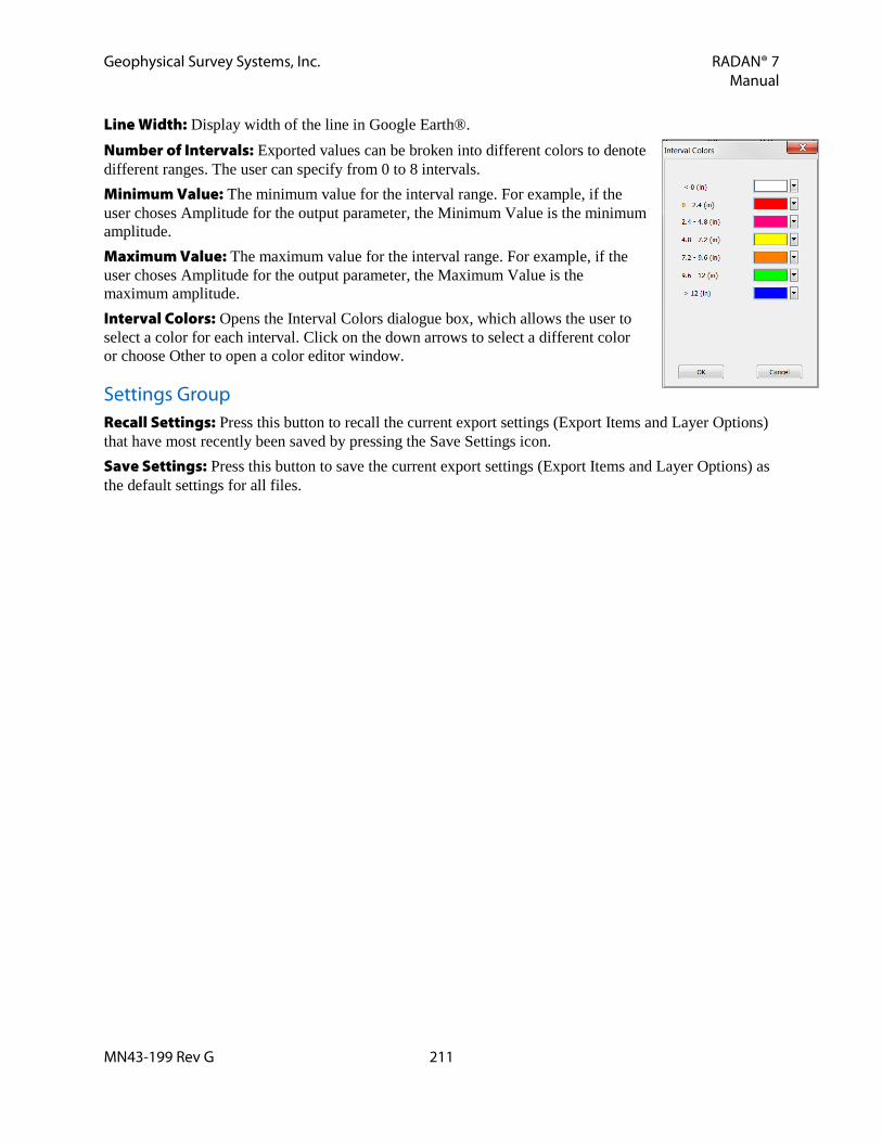
Geophysical Survey Systems, Inc. RADAN® 7 Manual
MN43-199 Rev G 211
Line Width: Display width of the line in Google Earth®. Number of Intervals: Exported values can be broken into different colors to denote different ranges. The user can specify from 0 to 8 intervals. Minimum Value: The minimum value for the interval range. For example, if the user choses Amplitude for the output parameter, the Minimum Value is the minimum amplitude. Maximum Value: The maximum value for the interval range. For example, if the user choses Amplitude for the output parameter, the Maximum Value is the maximum amplitude. Interval Colors: Opens the Interval Colors dialogue box, which allows the user to select a color for each interval. Click on the down arrows to select a different color or choose Other to open a color editor window.
Settings Group Recall Settings: Press this button to recall the current export settings (Export Items and Layer Options) that have most recently been saved by pressing the Save Settings icon. Save Settings: Press this button to save the current export settings (Export Items and Layer Options) as the default settings for all files.

Geophysical Survey Systems, Inc. RADAN® 7 Manual
MN43-199 Rev G 212

Geophysical Survey Systems, Inc. RADAN® 7 Manual
MN43-199 Rev G 213
Section 5: Basic Processing Tutorials This section offers step by step tutorials for some basic processing functions. For details on what each option does, refer to Section 3: Navigating through RADAN 7. Each of the tutorials use example data that can be downloaded from the GSSI Technical Support website. http://support.geophysical.com. Save the sample data on a computer.
Using the Proc. Lists Tab Adding Processes: How to add Categories and Processes within Categories in the Proc. List Tab for use over and over again.
1 Select the Proc. Lists tab from the Data, Processes, and Proc. Lists Pane.
2 Right-click on any of the Categories. The processes or categories will be placed under the selected category.
3 Select New.
4 Select: • Category: Creates a new category.
o Enter a Category Name and click on OK. • Process List: Creates processes under the
currently selected category. o Enter a Process List Name. o Select and Add all processes
to be included with this group. o Click on OK.
Editing or Deleting Processes: The user may Edit or Delete Categories or Process Lists by right-clicking on them with NO data files open. Export or Import Processes: The user may Export or Import Categories or Process Lists as XML files by right-clicking on them and exporting them for use on another computer, or importing them from another computer.

Geophysical Survey Systems, Inc. RADAN® 7 Manual
MN43-199 Rev G 214
Creating a Manual Grid These following steps will take the user through taking individual data files (.dzt) that were collected in a grid layout and combining them to create a 3D Grid file (.m3d). Files could be collected in the X direction only, Y direction only, or both X and Y directions. If the grid was collected using Quick 3D on the SIR system then just open the .B3D file and the grid will assemble automatically.
Sample Data: Grid___036.3DS
1 Prior to opening any data set the Source Directory (And Output Directory if Auto Save File is set to No) and the Vertical Units and Horizontal Units in the Global Settings.
2 Click the GSSI Button > Assemble Data File > 3D File.
3 Choose the location for the 3D Grid file.
4 Enter a filename for the Grid being created.
5 Click Save.
6 3D Grid Options: Enter the grid parameters. • 3D Filename: This is the file name created in Step
4 and will automatically be loaded. • Files in X/Y Direction: Fill in the tabs as
appropriate. For Grid___036 data were collected in both the X and Y Direction so both tabs need to be filled out.
• Starting (units): Both the X and Y Direction started at X = 0 and Y = 0.
• X-Length/Y-Length: Grid ___036 measured 50x50ft in both directions.
• # Profile Lines: 26 individual profiles (transects) were collected in both directions. • Line Spacing: Transects were spaced 2ft apart. This is automatically created by the # Profile
Lines and the line length. Use this to check for errors in the input parameters. • Line Order: Grid___036 was collected starting in the SW corner (bottom left) and transects were
collected in a zig-zag pattern. • Working Folder: This is where data are stored. Clicking this button will open a browser to
select a different directory. Select the folder for X or Y Direction files depending upon which tab is being filled out.
• Auto Load Files: Check this box to automatically load files from either the X or Y file folder.
7 Click OK.
Note: It is recommended that files collected in the X direction be put in a folder separate
from files collected in the Y direction.

Geophysical Survey Systems, Inc. RADAN® 7 Manual
MN43-199 Rev G 215
8 3-D File Creation: Shows the locations and orientations of the individual transects. Edit individual transects in this view if necessary. Can add or delete lines if they were not Auto-filled in the correct order.
9 Click OK when satisfied with the look of the grid. All of the files will be combined into a single grid file called Grid___036.DZT.

Geophysical Survey Systems, Inc. RADAN® 7 Manual
MN43-199 Rev G 216
Creating a Super Grid Combine multiple processed 3D Grids to create one “Super” 3D Grid. This will create a new file with the extension .S3D. Sample Data: Super3D > Grid___007-010.3DS
1 Prior to opening any data set the Source Directory (And Output Directory if Auto Save File is set to No) and the Vertical Units and Horizontal Units in the Global Settings.
2 Process each grid individually (see the Common Processing Steps later in this section). Individual grids can be created either by opening a .B3D file or manually assembling a grid as in the preceding tutorial.
3 Once each of the grids have been processed click the GSSI Button > Assemble Data File > Super 3D File.
4 Choose the location for the Super 3D Grid file.
5 Enter a filename for the Grid being created.
6 Click Save.
7 Click Add File to retrieve individual grids.
8 File Parameters
• Filename: Click Filename to browse and retrieve each grid.
• Starting (X,Y) Coords: Enter the X,Y starting position for each grid. o Grid___007: Starting (X,Y) Coords = (0,0) o Grid___008: Starting (X,Y) Coords = (0,10) o Grid___009: Starting (X,Y) Coords = (10,0) o Grid___010: Starting (X,Y) Coords = (20,0)

Geophysical Survey Systems, Inc. RADAN® 7 Manual
MN43-199 Rev G 217
• If necessary, a grid can be Rotated, Flipped Horizontally, and/or Flipped Vertically, depending on how it was collected relative to the coordinates of the other grids being assembled.
• Click OK when done. • The Super 3-D File Creation window
should look like the image to the right.
9 Click OK when satisfied with the look of the grids. All of the individual grids will be combined into a single grid file.

Geophysical Survey Systems, Inc. RADAN® 7 Manual
MN43-199 Rev G 218
Appending Files Append separate profiles to create one file. Sample Data: Grid___009.3DS
1 Prior to opening any data set the Source Directory (And Output Directory if Auto Save File is set to No) and the Vertical Units and Horizontal Units in the Global Settings.
2 Click the GSSI Button > Assemble Data File > Append Files.
3 Choose the location of the files being appended.
4 Enter a filename for the Append Files output.
5 Click Yes to merge the databases together creating one long profile.
6 Click Next.
7 Choose to Append All to select all of the profiles from Grid___009.
8 Click Finish.

Geophysical Survey Systems, Inc. RADAN® 7 Manual
MN43-199 Rev G 219
Basic 3D Grid Navigation When viewing data in the 3D mode (Home Ribbon > 3D-View), there are many options available to assist in interpretation of the data and provide improved images for documentation purposes. Sample Data: Grid___009.3DS
1 Prior to opening any data set the Source Directory (And Output Directory if Auto Save File is set to No) and the Vertical Units and Horizontal Units in the Global Settings.
2 Open and process the Grid___009.B3D file as needed (i.e. Time Zero, Background Removal, and Migration).
3 Click on 3D-View from the Home Ribbon. The View Ribbon will automatically open.
4 Display Window: • Left Pane: Continues to display the individual profiles. To view different profiles use the left and
right arrows located to the bottom left of the 2D profile. • Right Pane: Displays the 3D Grid image.

Geophysical Survey Systems, Inc. RADAN® 7 Manual
MN43-199 Rev G 220
Right Click Display Options Right click on the 3D Grid and access Display Gain and Transfer. Test changing each of the settings to see how they affect the 3D Grid.
1 Click Display Gain and select the Gain that will best display the data. Can choose from nine preset values or create a Custom Display Gain. Display Gain = 0
Display Gain = 30
2 Click Transfer to change how the data are displayed. • Click Abs Value to display all
targets as a positive amplitude. • Click Negate to display all targets
as a negative amplitude.

Geophysical Survey Systems, Inc. RADAN® 7 Manual
MN43-199 Rev G 221
Zooming In/Out the 3D Grid Image 1 Click the mouse on the 3D Grid image.
2 Hold down the [Ctrl] key on the keyboard and press the up and down arrow keys. If there is a wheel on the mouse, use it to zoom in and out on the image.
Resizing the Display 1 Point to the vertical bar located between the 2D image and 3D image.
2 Hold the left mouse button down and move the bar left or right.
Comparing 2D Location with 3D Location 1 Hold the left mouse button down
while pointing at the 2D image in the left pane. Cross hairs appear in the 3D image that corresponds with the location of the cursor.
2 To view other profiles, click the left and right arrows located in the bottom left of the 2D pane.
Slicing Through the 3D Grid Image
There are two ways to slice the 3D Grid image.
1 Move the X, Y, and Z slices using the mouse: • Point to the X, Y, or Z slice with the mouse. • Hold down the [Ctrl] key on the keyboard. • Hold down the left mouse button, and move the mouse.
2 Use options in the 3D Volume Options Ribbon: • Use the X, Y, or Z-Slice Position sliders to move the chosen slice.

Geophysical Survey Systems, Inc. RADAN® 7 Manual
MN43-199 Rev G 222
Drawing Pipes 1 Click Free Draw in the 3D Volume Options
Ribbon > 3D Interactive Mode.
2 Draw a pipe: • Double-click on one end of a target. • Double-click the other end of the target.
3 Add additional pipes: • Click the New Target icon. • Repeat process for drawing the first pipe. • To draw additional pipes repeat the previous
steps.
4 As new pipes are added, note the pipe information located in the Free Draw Groups Tab in Table Pane located at the bottom of the screen. The following options can be modified.
• Choose whether or not to display the target. • Choose the color of the target. • Choose the pixel size of the target. • Choose whether or not the target will display with a black outline. • Choose the diameter of the target. • Choose to link the two dots.
5 Right click on a pipe and select Delete to delete a pipe.
6 Click the GSSI Button > Export. • Save as an image file (.JPG, .BMP, or .PNG). • Save as AutoCAD format (.DXF).

Geophysical Survey Systems, Inc. RADAN® 7 Manual
MN43-199 Rev G 223
Interactive Processing This section describes the basic processing steps for picking layers and/or targets in data. Used primarily for RoadScan and BridgeScan, this can be used for any application and is also available in the 2D Interactive Ribbon. The layers and targets created are exported to a comma delimited ASCII file for use in any third party software. If GPS was collected with the data, targets and layers can be exported to a KML file for use with Google Earth.
Sample Data: FLOOR.DZT
1 Open FLOOR.DZT.
2 Click 2D Interactive Ribbon.
3 Click Add or Edit to turn on Interactive Mode.
Target Picking 1 Pick Type: Select Target.
2 Focus: Select Rebar (this will be the only option available to start).
3 Pick Polarity: Select Positive since the targets of interest in FLOOR.DZT are positive.
4 Search Width: Use the default search width of 9 pixels.
5 Click on the Single Point icon.
6 Position the mouse over the area where the pick is to be added. • Click the left mouse button to add target picks. • Click the right mouse button to delete target picks.
7 Click the New Target icon.
8 Click the Select Block icon.
9 Expand the block over a group of targets in the 2D display.
10 Right click inside of the block and choose Add Points.
11 Click the New Target icon.
12 Click the Select Range icon.
13 Size the height of the box, the width is automatically set to be the length of the profile, to encompass the targets.
14 Right click inside of the range and choose Add Points.

Geophysical Survey Systems, Inc. RADAN® 7 Manual
MN43-199 Rev G 224
Layer Picking Tools 1 Pick Type: Select Layer.
2 Focus: Select Layer 1 (this will be the only option available to start).
3 Pick Polarity: Select Positive since the targets in FLOOR.DZT are positive.
4 Search Width: Use the default search width of 9 pixels.
5 Display Gain: Adjust the Display Gain so that the layer of interest is identifiable.
6 Click on the Select Block or Select Range icon.
7 Adjust the block so that it encompasses the layer. • Click the left mouse button to add layer picks. • Click the right mouse button to delete layer picks.
8 Select Layer 2 from the Focus menu.
9 Click the EZ Tracker icon.
10 Click Start.
11 Click once with the left mouse button at the beginning of a layer.
12 Click again at the end of a layer. All of the points in between will be filled in. The EZ Tracker is more accurate when the mouse clicks are closer together.
13 Click Stop and Start to end one section of the layer and begin another.

Geophysical Survey Systems, Inc. RADAN® 7 Manual
MN43-199 Rev G 225
Ground Truth 1 Click on the Ground Truth icon.
2 Position the mouse over the top of a target. Choose any of the individual pieces of wire mesh from the example.
3 Click the top of the target located at approximately 14ft with the left mouse button.
4 Select Depth: A new menu will open. Enter a depth of 0.5ft. The depth is found by measuring to a known target, such as taking a core sample.
5 A ground truth point will be added to the 2D profile and the Interactive screen that appears below the data. A new entry will also be made to the Target Ground Truth tab in Table Pane.
6 Change Pick Velocity: Once a Ground Truth point is added to the data it can be used to adjust the velocity of adjacent target or layer picks. • Use Select Block to choose a group of
picks. • Right click within the block and choose
Pick Mod. Options > Change Pick Velocity.
• Choose Core Data from the Velocity Calc. menu.
• Click OK and this will apply the nearest Core Data (i.e. Ground Truth) information to the selected picks.

Geophysical Survey Systems, Inc. RADAN® 7 Manual
MN43-199 Rev G 226
Time Zero Correction Sample Data: EXCAVATION1.DZT
1 Open EXCAVATION1.DZT
2 Click on Easy Processing > Time Zero or click on the Processing > Time Zero.
3 Grab the first Positive Peak of the scan trace and adjust it to the top. The peak of the first positive wave will be bisected by the horizontal line at 0.0.
4 Click on Apply to test the correction and once satisfied with the result click OK.

Geophysical Survey Systems, Inc. RADAN® 7 Manual
MN43-199 Rev G 227
FIR Filtering Sample Data: BandPass.dzt
Background Removal Background noise, often seen as horizontal banding, may be removed using the FIR Filter. Always perform Time Zero Correction prior to Background Removal.
1 Open BandPass.dzt and perform a Time Zero Correction.
2 Click on the Processing Tab > FIR Filter.
3 Select TRIANGLE from the Filter Filters > Design menu.
4 Select BKGR REMOVAL from the FIR Filters > Horizontal > Type menu.
5 Choose the filter Length. For this file choose the maximum number of scans in the profile, 1307, for a full pass filter. • To determine the maximum
number of scans click the left mouse button once over the 2D profile data.
• Scroll the mouse of the far right side of the data. At the bottom of the screen a Scan number will appear.
6 Click on Apply to test the process and OK when satisfied with the results.

Geophysical Survey Systems, Inc. RADAN® 7 Manual
MN43-199 Rev G 228
Frequency Filtering Removes High Frequency vertical noise.
1 Open BandPass.dzt. Perform a Time Zero Correction and Background Removal.
2 Right Click in the data
3 Click on Transfer > Spectrum.
4 Change Display Gain to 0.
5 Determine the unwanted frequencies, which will normally appear bright white lines running horizontally through the data. For this file there is a bright white line at approximately 135MHz.
6 Click on the Processing > FIR Filter.
7 Select TRIANGLE from the Filter Filters > Design menu.
8 Enter 150MHz as the High Pass value to filter out the unwanted frequency identified in the Spectrum view.
9 Click on Apply to test the process and OK when satisfied with the results.

Geophysical Survey Systems, Inc. RADAN® 7 Manual
MN43-199 Rev G 229
Migration Sample Data: New_Pit/GRID___001.3DS/GRID___001.B3D
Constant Velocity Migration 1 Open New_Pit/GRID___001.3DS/GRID___001.B3D.
2 Perform a Time Zero Correction on the data.
3 Change the color table to something other than greyscale.
4 Increase the Display Gain to 12.
5 Click on Processing > Migration.
6 Position the ghost hyperbola over one of the real hyperbolas in the profile.
7 Adjust the tails of the ghost hyperbola to match the edges of the real hyperbola using the mouse.
8 Adjust the two vertical lines to encompass the beginning and end of the hyperbolic tails using the mouse.
9 Click on Apply to test the process. If the migration is successful the tails of the hyperbolas will collapse and all that will remain is a dot, which represents the top of the target.
10 Readjust the shape of the ghost hyperbola as necessary to create the target dot.
11 Click OK when satisfied with the results.

Geophysical Survey Systems, Inc. RADAN® 7 Manual
MN43-199 Rev G 230
Variable Velocity Migration 1 Open New_Pit/GRID___001.3DS/GRID___001.B3D
2 Perform a Time Zero Correction on the data.
3 Change the color table to something other than greyscale.
4 Click on Processing > Migration.
5 Select Profile L018. Use the arrows at the bottom left of the Linescan view to cycle through different profiles.
6 Double click on the black box that appears in the Velocity Plot.
7 Position the ghost hyperbola over the shallowest hyperbolas in the profile.
8 Adjust the tails of the ghost hyperbola to match the edges of the real hyperbola using the black box in the Velocity Plot.
9 Adjust the two vertical lines to encompass the beginning and end of the hyperbolic tails using the mouse.
10 Double click outside of the first black box in the Velocity Plot to create a second black box. This will bring up a second ghost hyperbola.
11 Position the second ghost hyperbola over the next hyperbola in depth in the profile.
12 Adjust the tails of the second ghost hyperbola to match the edges of the real hyperbola using the black box in the Velocity Plot.
13 Adjust the two vertical lines to encompass the beginning and end of the hyperbolic tails using the mouse.
14 Double click outside of the second black box in the Velocity Plot to create a third black box. This will bring up a third ghost hyperbola.

Geophysical Survey Systems, Inc. RADAN® 7 Manual
MN43-199 Rev G 231
15 Position the third ghost hyperbola over the next hyperbola in depth in the profile.
16 Adjust the tails of the third ghost hyperbola to match the edges of the real hyperbola using the black box in the Velocity Plot.
17 Adjust the two vertical lines to encompass the beginning and end of the hyperbolic tails using the mouse.
18 Click on Apply to test the process. If the migration is successful the tails of the hyperbolas will collapse and all that will remain is a dot, which represents the top of the target.
19 Readjust the shape of the ghost hyperbola as necessary to create the target dot.
20 Click OK when satisfied with the results.

Geophysical Survey Systems, Inc. RADAN® 7 Manual
MN43-199 Rev G 232
CMP Velocity Analysis and Migration Sample Data: CMP.DZT and BEDROCK.DZT To perform Velocity Analysis, data must first have been collected at multiple offsets using a bistatic antenna configuration and the common-midpoint (CMP) method. To estimate velocity from a CMP gather, collect GPR data using a bistatic antenna configuration in Point mode with Stacking turned on. Initially, transmitting and receiving antennas start off adjacent to one another at the zero offset position. Because of the size of the antennas’ housings, transmitting and receiving antennas are never at a true zero offset position. Rather, the initial offset is the distance from the symmetrical reference - i.e., the zero offset position- to the antenna’s centerline. Data are then collected at multiple offsets as the antennas are moved symmetrically apart from the zero offset position. The output data quality improves significantly using a large number of small offsets and more stacking but increases the collection time. The operator will have to decide the best utilization of time when establishing the best offset interval, the number of stacks per measurement, and number of offsets, versus the desired quality of data output.
1 Prior to opening any data set Global Parameters as follows: • Auto Save File: Yes • Source Directory: Set to the location of Tutorial Data. • Vertical and Horizontal Units: Meters
2 Open CMP.DZT.
3 Click on Processing > Velocity Analysis.
4 Configuration:
• Step: 0.20 meters. The step interval distance the antennas are moved apart each time data is acquired during the CMP gather.
• Offset: 0.20 meters. The initial distance between the transmitting and receiving antennas at their zero-offset positions when they are at their closest spacing during the CMP gather. Because of the antenna housing this value will always be greater than zero.
5 Analysis:
• Min Velocity: This is the minimum velocity expected based upon the area where the CMP gather was completed. Adjust this value after running Recalc to improve the display of the velocity in the diagram plot if necessary.
• Max Velocity: This is the maximum velocity expected based upon the area where the CMP gather was completed. Adjust this value after running Recalc to improve the display of the velocity in the diagram plot if necessary.
• T0 Method: Auto. • T0 Value: Does not change since T0 Method is set to Auto.
6 Adjust the left box that appears in the top left corner of the profile in the Linescan Display.

Geophysical Survey Systems, Inc. RADAN® 7 Manual
MN43-199 Rev G 233
7 Click the Recalc button and the program will calculate the estimated velocities of the layers present in the data.
8 Variable Velocity Analysis: Once the parameters under the Velocity Diagram are set the user can create a variable velocity curve based upon the maximum velocity points. • Double-click with the left mouse on the velocity diagram plot. • Position the newly created box over the highest maximum velocity. • Continue to double-click to create additional boxes to match with
maximum velocity spots.
9 Velocity Analysis Tab: The Tables Pane updates as more velocity points are added in the Velocity Diagram.
10 Click Save to create a velocity file, CMP.VLC, for use in a Migration process on the file collected over the same area as the CMP gather.
11 Open BEDROCK.DZT
12 Click on Processing > Migration.
13 Open Velocity File • Load Vel. File: Double-click in the text field located to the right of Load Vel. File. • Open CMP.VLC
14 Perform hyperbolic fitting as described in the Migration Tutorial.
15 Click OK to run the Migration using the velocity file created using CMP Velocity Analysis.

Geophysical Survey Systems, Inc. RADAN® 7 Manual
MN43-199 Rev G 234
Distance Normalization This will adjust the horizontal scale for data collected in Time Mode. Sample Data: DistNorm.dzt
1 Open DistNorm.dzt
2 Click on Processing > Distance Normalization.
3 In the Properties Pane > Header note that Scans/Unit and Units/Mark information is entered from the field notes when collecting the data. • Scans/Unit: 25 • Units/Mark: 5
4 Remove the first user mark from the data. The first user mark should appear where the data collection began, which is the second user mark for DistNorm.dzt. • Select the Way Points tab in the Tables Pane at the bottom of the screen. • Select the first User Mark using the mouse. • Uncheck the User Mark box that corresponds with the first User Mark from the Waypoints Tab in
the Tables Pane.
5 Select Yes for Apply to User Marks.
6 Click on OK to run the Distance Normalization.

Geophysical Survey Systems, Inc. RADAN® 7 Manual
MN43-199 Rev G 235
Deconvolution Remove horizontal noise that is not consistent across the entire profile, which can be removed using Background Removal, or ringing noise. Sample Data: TANKSINWATER.dzt
1 Open TANKSINWATER.dzt
2 Click on Processing > Deconvolution.
3 Right click on the vertical scale and change the scale to Samples.
4 While holding the left mouse button down, place the cursor in the middle of the first peak and note the number of samples located at the bottom of the RADAN 7 window ( example: 64.88).
5 Continue to hold the Left Mouse Button down, place the cursor on the next positive peak and note the sample number (example: 88.86).
6 Note the difference of the two numbers. This is the number of samples that make up 1 pulse length (example: 88.86-64.88 = 23.98).
7 In the Deconvolution Process Pane • Operator Length – The number noted in Step 6 (example: 23.98). • Prediction Lag – Start with about ½ of the Operator Length and gradually work lower. The
lower the number, the more noise will be produced in the Deconvolution output. • Prewhitening % - Leave as default. • Overall Gain - Change the Display Gain to improve contrast in the processed data.
8 Click on Apply to test the process and OK when satisfied with the results.

Geophysical Survey Systems, Inc. RADAN® 7 Manual
MN43-199 Rev G 236
Note: After removing the horizontal bands the data can be further improved by applying an FIR frequency filter.

Geophysical Survey Systems, Inc. RADAN® 7 Manual
MN43-199 Rev G 237
Horizontal Scaling This process is used to shrink or expand a profile by extracting or interpolating between scans. Sample Data: Strats.dzt
1 Open Strats.dzt
2 Click on Processing > Horizontal Scaling.
3 Stacking: This will average a specified number of scans and replace those scans with the average scan. • Input 3 as the Stacking Value. • Click Apply to test this function.
4 Skipping: This will skip and delete scans at a specified interval. • Input 1 as the Skipping Value. • Click Apply to test this function.
5 Stretching: This will add scans at a specified interval. • Input 2 as the
Stretching Value. • Click Apply to test
this function.
6 Click OK when satisfied with any of the results.

Geophysical Survey Systems, Inc. RADAN® 7 Manual
MN43-199 Rev G 238
Surface Normalization Surface Normalization corrects for topographic changes. Sample Data: SurfaceNorm.dzt
1 Open SurfaceNorm.dzt
2 Click on Processing > Surface Normalization.
3 Elevation values have to be manually assigned to the markers using Edit Markers if they are not imported with GPS data. When entered, elevation data will be stored in the Way Points tab of the Table Pane.
4 Normal Level: Since Auto Level will be set to Yes this option is not available.
5 Vertical Scale: Start at a 1:1 scale.
6 Auto Level: Set to Yes
7 Click Apply and Reset. Then make adjustments to Vertical Scale as necessary. For this example a 1:2 scale works best.
8 Click OK once desired results are achieved.
Before Surface Normalization.
After Surface Normalization.
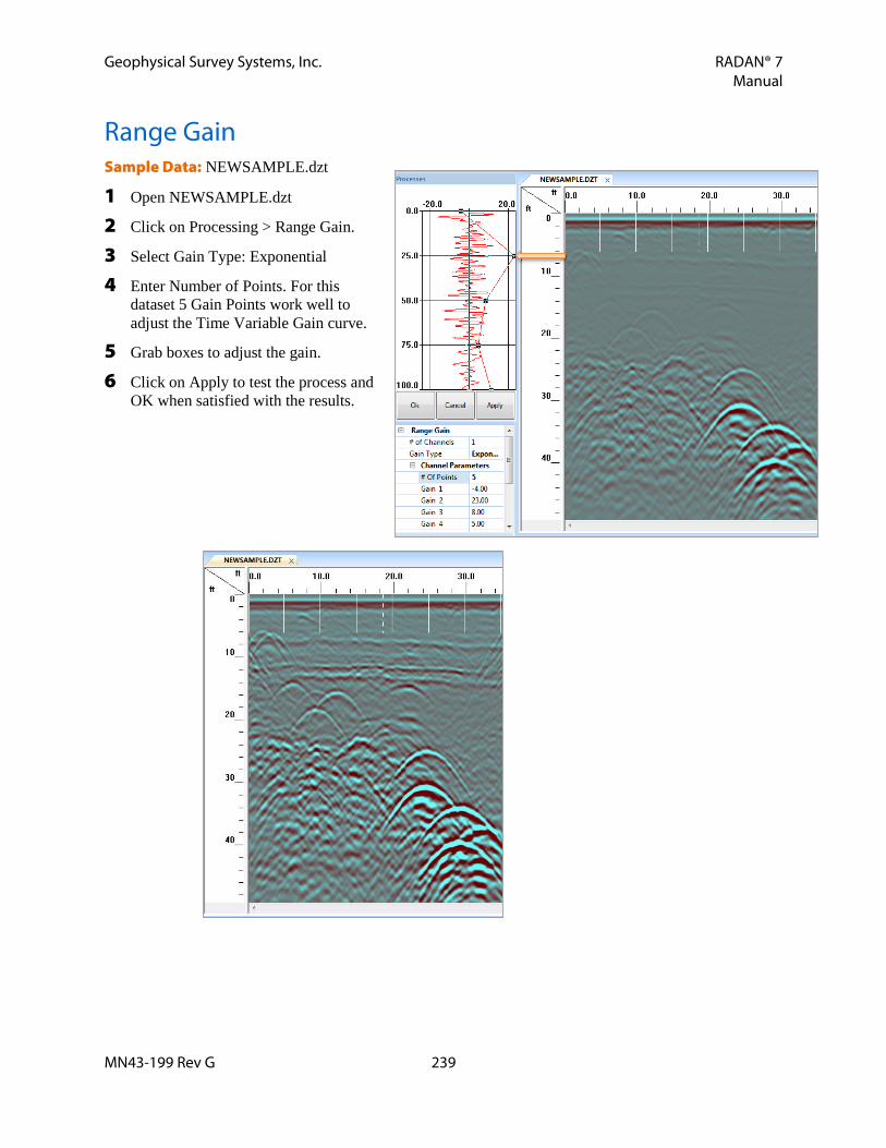
Geophysical Survey Systems, Inc. RADAN® 7 Manual
MN43-199 Rev G 239
Range Gain Sample Data: NEWSAMPLE.dzt
1 Open NEWSAMPLE.dzt
2 Click on Processing > Range Gain.
3 Select Gain Type: Exponential
4 Enter Number of Points. For this dataset 5 Gain Points work well to adjust the Time Variable Gain curve.
5 Grab boxes to adjust the gain.
6 Click on Apply to test the process and OK when satisfied with the results.

Geophysical Survey Systems, Inc. RADAN® 7 Manual
MN43-199 Rev G 240
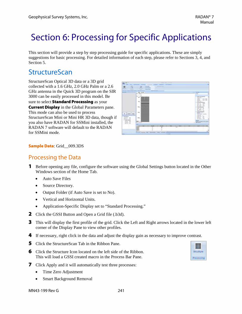
Geophysical Survey Systems, Inc. RADAN® 7 Manual
MN43-199 Rev G 241
Section 6: Processing for Specific Applications This section will provide a step by step processing guide for specific applications. These are simply suggestions for basic processing. For detailed information of each step, please refer to Sections 3, 4, and Section 5.
StructureScan StructureScan Optical 3D data or a 3D grid collected with a 1.6 GHz, 2.0 GHz Palm or a 2.6 GHz antenna in the Quick 3D program on the SIR 3000 can be easily processed in this model. Be sure to select Standard Processing as your Current Display in the Global Parameters pane. This mode can also be used to process StructureScan Mini or Mini HR 3D data, though if you also have RADAN for SSMini installed, the RADAN 7 software will default to the RADAN for SSMini mode. Sample Data: Grid__009.3DS
Processing the Data 1 Before opening any file, configure the software using the Global Settings button located in the Other
Windows section of the Home Tab. • Auto Save Files • Source Directory. • Output Folder (if Auto Save is set to No). • Vertical and Horizontal Units. • Application-Specific Display set to “Standard Processing.”
2 Click the GSSI Button and Open a Grid file (.b3d).
3 This will display the first profile of the grid. Click the Left and Right arrows located in the lower left corner of the Display Pane to view other profiles.
4 If necessary, right click in the data and adjust the display gain as necessary to improve contrast.
5 Click the StructureScan Tab in the Ribbon Pane.
6 Click the Structure Icon located on the left side of the Ribbon. This will load a GSSI created macro in the Process Bar Pane.
7 Click Apply and it will automatically test three processes: • Time Zero Adjustment • Smart Background Removal

Geophysical Survey Systems, Inc. RADAN® 7 Manual
MN43-199 Rev G 242
• Auto Amplitude Correction (Migration) You may need to increase the Display Gain by right clicking on the data or in the Display section of the Home ribbon.
8 Check the outcome of the processing. The hyperbolas should collapse to dots. If you still see hyperbolas, adjust the Dielectric Constant value lower and retry. Inverted hyperbolas mean you need to adjust the value higher. You will notice the Velocity value adjust accordingly.
9 Click OK once desired results are achieved.
View Depth Slices While in the StructureScan Ribbon the user can view depth slices. This view shows the data from the top and also offers the ability to slice through the data.
1 Click the View Depth Slices Icon.
2 This opens a top-down view of the data.
3 Make adjustments as follows:

Geophysical Survey Systems, Inc. RADAN® 7 Manual
MN43-199 Rev G 243
• Slice Depth: Slice the Z slice up and down. Uncheck Full Thickness Slice prior to using Slice Depth. You can also hold down the Control (CTRL) button on your keyboard and, using the left mouse button, click and hold to drag the data up and down.
• Slice Thickness: Adjust the thickness of the slice. This represents the amount of data in the Z plane that you will see as a single image. The thicker the slice, the more data will be shown and it may be difficult to note relative depth differences in the objects.
• Maximum Depth: Adjust the Depth of the data • When viewing from the very top of the data, may
either view as a Full Thickness Slice, or turn this feature off.
4 Right-click the Depth Slices View: • Adjust the display gain. Higher values will make the data brighter. • Drill a hole. This will place a cylindrical, green marker in the data with the center point being
where you clicked. You can select a desired hole diameter. This is meant as a place holder in order to help you spot any potential impacts of a core drilled at that location.
5 Print this image, or save it as a jpeg file. • From the Home Ribbon, click Print to print. • Click the GSSI Button, then click Export, and click Save as a JPG file to save as a picture file.
3-D View 1 Turn off View Depth
Slices in the StructureScan Ribbon.
2 Clicking on the Home Ribbon tab provides options for viewing and manipulating the 3D cube. Please refer to Section 5, Basic 3D Grid Processing for options in this view.

Geophysical Survey Systems, Inc. RADAN® 7 Manual
MN43-199 Rev G 244
RoadScan Sample Data: ROADSCAN001.dzt and ROADSCAN002.dzt
1 Prior to opening any data, select Global Settings from the Other Windows section of the Home ribbon. Find Current Display in the properties pane on the right and set it to RoadScan.
2 Once the RoadScan module is open select Global Settings again and confirm or modify the following settings prior to opening any data. • Auto Save File: Yes • Source Directory: Location of Tutorial Data. • Vertical Units: inches/cm • Horizontal Units: feet/m • Auto-Switch Display: Set to No. RADAN will kick you back into Standard Processing when
you open if file if you forget to set this to No. • You may also find it easier to view the data using an exponential Color Transform. Select Color
Xforms from the Display section of the Home ribbon and set it to Transform 1.
Creating the Calibration File In order to process RoadScan data a metal plate calibration file needs to be created.
1 Click the GSSI Button and open the metal plate calibration file (bumper jump), ROADSCAN001.DZT.
Note: If you open data collected with the SIR 30 RADAN will automatically process the raw data with the filters and gain settings you had implemented during collection. This includes the customer FIR filters from the Horn antennas. GSSI recommends that you allow this process to finish before proceeding. If you have Auto Save set to No, you will be prompted to save the file when it is completed.

Geophysical Survey Systems, Inc. RADAN® 7 Manual
MN43-199 Rev G 245
2 Click the RoadScan Tab in the Ribbon Pane.
3 Click the Horn Calibration Icon. This will open the Horn Calibration process in the Process Bar Pane. Set Automatic Mode to No so that the following options appear: • Use Air Wave File: (This is not common). An air wave file is required for the older bistatic Horn
antennas (models 4208 and 4205). Set to No for any 4108, 4105, 41000S, or 42000S antennas. • # of Channels: Set this to the number of channels of data that you have. Typically this will be
equal to the number of antennas used in your survey. • Channel: Set the Antenna Type and Serial Number of the antenna. These will already be filled in
if you are using a Smart antenna.
4 Click OK. This will create a calibration file (.CZT) for the road data collected. Take note of the CZT file’s name.
5 Close all files.
Processing the Road File 1 Click the GSSI Button and open ROADSCAN002.DZT.
2 Click the Reflection Picking Icon.
3 Calibration File Select Method: Auto Select. This will select the CZT file corresponding to the smart antenna’s serial number. If this antenna was not a smart antenna, than choose User Select and browse to find the correct CZT file.
4 Automatic Mode: Set to Yes. The reflection picking process has a number of automatic filters designed to remove noise from your data.
5 Click OK to apply the Calibration File to the Road File

Geophysical Survey Systems, Inc. RADAN® 7 Manual
MN43-199 Rev G 246
After Reflection Picking
Layer/Target Picking 1 Click the Interactive Icon.
2 Using the Interactive Pane of the RoadScan Ribbon, Begin entering picks for each layer. Refer to Section 3, RoadScan Ribbon or Section 4, or Section 5, Interactive for detailed information how to pick layers and targets.
3 When complete, save the comma delimited ASCII file for use in other 3rd party software. The CSV File selection under the Export Group will save an ASCII file.
Picking Layer

Geophysical Survey Systems, Inc. RADAN® 7 Manual
MN43-199 Rev G 247
BridgeScan This is for data collected specific to determine bridge deterioration. Sample Data: EHB.dzt
1 Prior to opening any data, select Global Settings from the Other Windows section of the Home ribbon. Find Current Display in the properties pane on the right and set it to Horn BridgeScan.
2 Once the RoadScan module is open select Global Settings again and confirm or modify the following settings prior to opening any data. • Auto Save File: Yes • Source Directory: Location of Tutorial Data. • Vertical Units: inches • Horizontal Units: feet
Preparing the Data 1 Click the GSSI Button and Open EHB.DZT.
2 This will display the first profile of the bridge. Click the Left and Right arrows located in the lower left corner of the Display Pane to view other profiles.
3 Right click in the data and adjust the display gain to increase the contrast.
4 Click the BridgeScan Tab in the Ribbon Pane.

Geophysical Survey Systems, Inc. RADAN® 7 Manual
MN43-199 Rev G 248
5 Select Deterioration Mapping. This process will correct the time zero of the data as well, apply picks to the rebar, and create a comma delimited ASCII file for export. This will open the Deterioration Mapping process in the Process Bar Pane. o Select Concrete Overlay o Time Zero Amplitude Threshold. o Velocity (Top Layer/Ft).
6 Click Apply to test the process.
7 If necessary, click Reset to make any adjustments to the three values and click Apply again. The
Dielectric Constant is most often the value that needs adjusting. If the individual pieces of reinforcement do not appear as dots then the Dielectric Constant needs to either be changed. If the pieces of reinforcement look like a “U” then the Dielectric Constant should be increased. If they appear as upside-down “U”s then the value should be decreased. Continue adjusting until achieving the desired results.
8 Click OK.

Geophysical Survey Systems, Inc. RADAN® 7 Manual
MN43-199 Rev G 249
Editing Target Picks 1 Turn on Interactive Mode under the BridgeScan
Ribbon.
2 Using the Interactive Group, make any adjustments to the picks generated by the Deterioration Mapping process. Please refer to Section 3, BridgeScan Ribbon or Section 4, or Section 5, Interactive Processing for detailed information on how to pick targets.
3 When complete, save the comma delimited ASCII file for use in other 3rd party software. The CSV File selection under the Export Group will save an ASCII file. Select the following options to facilitate exporting. • Modify Existing • GSSI – BridgeScan – Deterioration (Local Coords or Lat Long Coors) • Way Points and Targets • No Filtering

Geophysical Survey Systems, Inc. RADAN® 7 Manual
MN43-199 Rev G 250

Geophysical Survey Systems, Inc. RADAN® 7 Manual
MN43-199 Rev G 251
Appendix A: Sample Data These examples are presented for informational use only. Conditions will vary and may cause the images to look different from the data shown here. Examples 1 – 4 are data collected with a 1600 MHz antenna. Examples 5 – 8 are data collected with a 400 MHz antenna.
Example 1: Concrete Block Data
Example 2: Rebar Data This is an example of rebar. Note the distance between the peaks is approximately 8 inches. Also note the approximate depth, that they tend to be at a constant depth over the length of this profile, and the brightness of the hyperbolas.
User Marks entered during collection to identify the ends of each block (black
Filled cell with rebar
2 voids within the blocks

Geophysical Survey Systems, Inc. RADAN® 7 Manual
MN43-199 Rev G 252
Example 3: Mesh Data This is an example of wire mesh. Note the distance between the peaks is approximately 6 inches. Also note the approximate depth, the brightness of the hyperbolas, and the mesh varies in depth more than the rebar example above.
Example 4: PVC This is an example of two PVC pipes located above rebar. Note the plastic pipes tend to be dimmer than rebar and that the first dominant color is black instead of white, which indicates a reflection that begins with a negative and not positive polarity. The PVC is also shallower than the rebar.

Geophysical Survey Systems, Inc. RADAN® 7 Manual
MN43-199 Rev G 253
Example 5: Bank of Conduits This profile shows a bank of conduits feeding into an industrial building. Note the dipping edge of a trench cut to the upper left of the conduits.
Example 6: Empty PVC Pipe
This image shows three drain lines. The one in the middle (depth-wise) is an 8” PVC pipe (empty).

Geophysical Survey Systems, Inc. RADAN® 7 Manual
MN43-199 Rev G 254
Example 7: Water Main This image shows data collected across a road, looking for a water main.
Example 8: Culvert This image shows data collected along a driveway next to a business. This shows a concrete culvert with two conduits running through the bottom of the culvert.

Geophysical Survey Systems, Inc. RADAN® 7 Manual
MN43-199 Rev G 255
Appendix B: GSSI Naming Convention When Auto Save to Yes under the Properties Pane, GSSI will automatically name the processed files and place them in an automatically created PROC folder inside the source folder. The naming convention for the processed files is as follows:
• The original file is represented by <FileName>.dzt. Once this file is processed, a new file is created in the PROC folder and named <FileName> P1.dzt.
• If the ORIGINAL file is processed again, then each processed file will increment by 1. • If a processed file is processed again, another digit will be added to the name of the processed file
to create a new file in the PROC folder. Example: If a processed file <FileName> P1.dzt, is processed again then the new file is named <FileName> P11.dzt.
The figure below diagrams the GSSI naming convention:

Geophysical Survey Systems, Inc. RADAN® 7 Manual
MN43-199 Rev G 256

Geophysical Survey Systems, Inc. RADAN® 7 Manual
MN43-199 Rev G 257
Appendix C: Dielectric Constants The relative dielectric permittivity is a unit-less measure of the capacity of a material to store a charge when an electric field is applied. The dielectric constant is the real part of dielectric permittivity, as it is normalized to air. Dielectric constant values vary from material to material. In dry materials the dry bulk density primarily influences the dielectric constant. In partially saturated or saturated soils the dielectric constant is primarily determined by the water content. Radar energy is reflected at boundaries of electrically dissimilar materials where there is a contrast in the dielectric constants (i.e., where there is electrical impedance). These boundaries typically occur at stratigraphic boundaries, but may occur at the water table and within stratigraphic units where changes in electrical properties occur. The chosen value of the dielectric constant is directly related to velocity and defines the relationship between time and depth. In resistive soils, those with conductivities less than 20 millimhos per meter, the average soil velocity may be approximated by:
• This equation is not valid in conductive soils (such as clays) or soils with conductive pore fluids (such as brackish and conductive groundwater).
• When a dielectric constant value is input in the header, RADAN 7 makes the assumption that this value is valid throughout the entire file, which may not be representative.
• The dielectric constant may be changed to evaluate the effect of different velocity assumptions of the location of features.
The dielectric constant may be determined from: • On-site calibrations over targets of known depth. Use Ground Truth in Interactive Mode to
calibrate over known depths in RADAN 7. • Common depth point or midpoint (CDP or CMP) calibrations using bistatic antennas over a
reflector of known depth (such as the water table). • Estimated velocities or dielectric constants observed at similar sites. • Hyperbolic fitting using the Migration Processing method (see Section 5).
VmCEr=
Vm is the average soil velocity (m/s)
C is the speed of light or 2.998 x 10 8 m/s
Er is the dielectric constant

Geophysical Survey Systems, Inc. RADAN® 7 Manual
MN43-199 Rev G 258
Material Dielectric Constant
Material Dielectric Constant
Air 1 Wet Sandstone 6 Snow Firn 1.5 Wet Granite 6.5 Dry Loamy/Clayey Soils 2.5 Travertine 8 Dry Clay 4 Wet Limestone 8 Dry Sands 4 Wet Basalt 8.5 Ice 4 Tills 11 Coal 4.5 Wet Concrete 12.5 Asphalt 5 Volcanic Ash 13 Dry Granite 5 Wet Sands 15 Frozen Sand & Gravel 5 Wet Sandy Soils 23.5 Dry Concrete 5.5 Dry Bauxite 25 Dry Limestone 5.5 Saturated Sands 25 Dry Sand & Gravel 5.5 Wet Clay 27 Potash Ore 5.5 Peats (saturated) 61.5
Dry Mineral/Sandy Soils 6 Organic Soils (saturated) 64
Dry Salt 6 Sea Water 81 Frozen Soil/Permafrost 6 Water 81 Syenite Porphyry 6

Geophysical Survey Systems, Inc. RADAN® 7 Manual
MN43-199 Rev G 259
Appendix D: Glossary of Terms Antenna: A component of an impulse radar system designed to radiate radio waves (electromagnetic radiation) from Applied voltage impulses (transmitting antenna), or conversely, to intercept radio waves and convert them back into electrical impulses (receiving antenna). Antennas radiate or receive electromagnetic energy. Antenna Radiation Pattern: A plot of the intensity of the radiation received at a given radial distance from an antenna versus angle, relative to a given reference axis. The pattern is a three dimensional measure of the energy at a fixed radial distance from the antenna. Attenuation: A measure of the loss of radiated signal amplitude or signal energy as it progresses through a lossy medium. The loss can be due to a spreading loss as the wave expands out into the medium and also due to an ohmic loss, due to the finite conductivity of the medium. Background Removal: A digital signal processing function that filters by subtracting an average of a large number of scans from each individual scan. The result is horizontal changes in the data are accentuated while linear features (background) are suppressed. Backscatter: A portion of a radar's transmitted energy that is intercepted by a target, or other object and reflected (scattered) back in the radar's direction. Bandwidth: The band of frequencies occupied by the central lobe of the spectrum of an electromagnetic signal. Bandwidth is usually defined so that it includes most, but not all of the signal power. Generally, it includes the portion lying between the points at which the power has dropped to half that at the center of the band. Beamwidth: The angular width of a slice through the main lobe of the radiation pattern of an antenna. Bias: The amount by which the average of a set of values departs from a reference value. Bistatic: The survey method that utilizes two separate antennas at a constant distance. One antenna has a transmitter and the other contains a receiver sampler. With this method it is possible to transmit a higher power signal and receive reflections with a greater time delay. Common Depth Point (CDP) or Common Midpoint (CMP): Having the same midpoint between source and detector. Common Depth Point Method: A survey method that can be performed to calculate the electromagnetic velocity of a material. This is conducted by transmitting from one antenna and receiving from a second antenna at several known offsets (surface horizontal distance). Clutter: Unwanted reflections from the ground, from within the ground or from above the ground. In the case of ground penetrating radar (GPR), clutter may be produced by boulders, soil interfaces and other scatters that are not of interest. Clutter can also be produced within the radar system. Conductivity: The electrical conductivity of a dielectric material is a measure of the ease with which an electrical current can be made to flow through it. In the MDS system, the unit of conductivity is the Siemens per meter (S/m). Conductivity is the reciprocal of resistivity. The higher the conductivity of the subsurface materials, the greater the attenuation of the radar signal. Control Unit (C/U): An electronic instrument that interfaces a transducer (s) to recorders, processors, displays, survey wheel, power supply, etc. It also has controls to allow radar functions such as range, gain and filtering to be adjusted. A C/U can be analog, digital, or hybrid. Data Channel: A software channel on the control unit that displays and records a received signal. It is possible to have one transducer and four data channels with the same or varied processes.

Geophysical Survey Systems, Inc. RADAN® 7 Manual
MN43-199 Rev G 260
Decibel (db): A unit of measure for gain. A logarithmic unit used to express power ratios. One decibel equals 20 LOG (P2/P1). Decibels are also used to express voltage ratios. Deconvolution: A digital signal processing function designed to attenuate multiples and improve the recognition and resolution of reflected events. A process that restores a waveshape to the form it had before it underwent a linear filtering action (convolution). Delay Time: The amount of time the radar wave propagates through a material, reflects off an interface and returns to the receiver. Time lag introduced by either hardware (cable length, etc.) or software ( filter averaging, etc.). Depth of Penetration: In any medium, the radar wave is attenuated as it progresses due to losses that occur. At radar frequencies in a conductive material (sea water, metallic materials, clay soils, etc.) the rate of attenuation is very great and the wave may penetrate only a short distance (<1m) before being reduced to a negligibly small value. In a resistive dielectric earth material (fresh water, granite, quartz sand, etc.), where the losses are low, the depth of penetration can be quite great (>30m). Dielectric Constant: See Dielectric Permittivity. Dielectric Permittivity: Dielectric Permittivity is a property of an electrical insulating material (a dielectric) equal to the ratio of the capacitance of a capacitor filled with the given material to the capacitance of the identical capacitor filled with air. Earth materials are classified generally as conductors, semiconductors and insulators (dielectrics). A dielectric material is a poor conductor of electric current. The specific capacitance of a vacuum is Eo = 8.85 x 10⁻¹² Farads per meter. The relative dielectric constant, Er for air is 1 and is approximately 81 for fresh water. Dielectric Interface: A place in the subsurface of a dielectric material where the dielectric permittivity changes. Diffraction: The phenomenon that causes electromagnetic waves in the beam of a directional antenna to spread out. The bending of wave energy around obstacles without obeying Snell's Law. An event that occurs at the termination of curved topped, or steeply dipping reflectors that is characterized by a distinctive curved alignment. Diffuse: To break up and distribute the energy in an incident electromagnetic wave in many directions. Dipole: A simple antenna having two elements driven from the center of the antenna by a balanced source. Directivity: Ability of an antenna to concentrate transmitted energy in a given direction and to emphasize the returned energy received from that direction. Dynamic Range: The spread between the minimum signal at the input of a system, which produces a discernible change in the output and the maximum input that the system can handle without saturating. Measured in decibels (db). Echoes: Radar energy reflected from a given target or object. Electromagnetic Wave: A wave that is propagated by the mutual interaction of electric and magnetic fields. Radiant heat, light and radio waves, are electromagnetic waves. Finite Impulse Response (FIR) Filter: A digital signal processing function that convolves a finite length function (boxcar, triangle) with the data. Each data value is multiplied by the corresponding filter value and added together. FIR filters are digital filters and have no time delay. Frequency: The number of positive and negative voltage amplitude cycles that a pure unmodulated sine wave completes per second. The unit of frequency is Hertz (Hz).

Geophysical Survey Systems, Inc. RADAN® 7 Manual
MN43-199 Rev G 261
Frequency Domain: Mathematical realm in which the amplitudes of signals are expressed as functions of frequency, rather than time. The frequency spectrum of a time varying signal is obtained by translating the expression for the signal from the time domain to the frequency domain. Frequency Domain (FK) Filter or Velocity Filter: A digital signal processing function that discriminates on the basis of apparent velocity. Coherent arrivals with certain apparent velocities are attenuated. Fresnel Zone: The portion of a reflector from which reflected energy can reach a detector within one-half wavelength of the first reflected energy. Gain: A change in signal amplitude or power from one point in a circuit or system to another, often from system input to output. See Range Gain. Gigahertz: A unit of frequency. One GHz equals 109 Hz. GPR: Acronym for Ground Penetration Radar. GPS: Acronym for Global Positioning System. Hertz (Hz): A unit of frequency. One Hertz equals one cycle per second. High Pass Filter: A filter that passes without significant attenuation frequencies above some cutoff frequency while attenuating lower frequencies. The same as low-cut filter. Hilbert Transform: A digital signal processing function that determines the magnitude envelope, instantaneous phase and instantaneous frequency of a received signal. Horizontal Filter: A digital signal processing function that attenuates signals outside the filter function across adjacent scans. Infinite Impulse Response (IIR) Filter: A digital signal processing function that emulates an analog filter function. An IIR filter is a filter function that offsets the data in time. Interface: The common surface separating two different media in contact. A location in the subsurface where the dielectric constant changes. Isotropic Radiator: An antenna that radiates equally (both in amplitude and in phase) in all directions. The imaginary source of the radiation used as a reference for the gain of a directional antenna. Lateral Resolution: The ability of the system to resolve in a horizontal direction the smallest discernible target. This is a function of antenna frequency, scan rate and speed of travel. Low Pass Filter: A filter that passes frequencies below some cutoff frequency while substantially attenuating higher frequencies. Same as a high-cut filter. Magnetic Permeability: The magnetic permeability of a material is a measure of the difficulty of magnetization of the material in an external field. The magnetic permeability of earth materials is taken to be that of free space, = 4 x 10⁻⁷ Henrys per meter. Therefore, the relative permeability of earth materials is Ur = 1. Megahertz: A unit of frequency. One MHz equals 106 Hertz. Migration: A digital signal processing function that rearranges data so that reflections and diffractions are plotted at the locations of the reflectors and diffracting points rather than with respect to observation points on the profile. Migration by computer is accomplished by integration along diffraction curves (Kirchhoff migration), by numerical finite-difference downward-continuation of the wave equation and other algorithms. Monostatic: A survey method that utilizes a single transducer with either a single antenna with transceiver or a dual antenna transducer with separate electronics.

Geophysical Survey Systems, Inc. RADAN® 7 Manual
MN43-199 Rev G 262
Multiple: Also known as ringing. Wave energy that has been reflected more than once. In radar data multiples may occur when there is a large change in the dielectric permittivity or conductivity of the medium. A multiple can be identified by signals that have the same time delay as between the surface and the first reflector. Nanosecond: A unit of time. One nanosecond equals 10-9 seconds; one billionth of a second. Nearest Neighbor: This gridding method assigns the value of the nearest point to each grid node. This method is useful when data are evenly spaced, but need to be converted to a grid file. Alternatively, in cases where the data are nearly on a grid with only a few missing values, this method is effective for filling in the holes in the data. Noise: Unwanted, usually random, electrical or electromagnetic energy that interferes with the detection of wanted signals. The term is also applied to any unwanted random variations in the measured value of any quantity. PC: Acronym for Personal Computer. Permittivity: See Dielectric Permittivity. Phase: Degree of coincidence in time between a repetitive signal, such as a sine wave and a reference signal, having the same frequency. The angle of lag or lead of a sine wave with respect to a reference. Generally expressed in degrees. 360 degrees corresponds to the period of the signal. Point Reflector: A subsurface feature with electromagnetic properties different from its surroundings, whose dimensions are approximately the same as the fresnel zone of the radar wave. Polarization: The orientation of the electric and magnetic fields of an electromagnetic wave, such as a radio wave. By convention, the polarization of the wave is the direction of the electric field. If the polarization does not change as the wave propagates, the polarization is said to be linear. Power: A measure of the quantity of electric energy, commonly expressed in Watts. One watt equals one Joule per second. Profile: A graph showing the depth measurements as a vertical cross section of the medium along a horizontal line. PRF (Pulse Repetition Frequency): The number of pulses per second transmitted by a pulsed radar. Propagation: The outward spreading, or travel, of an electromagnetic wave, such as a radio wave. RADAR: RAdio Detection And Ranging. An electronic system that transmits electromagnetic energy and detects the location of reflected energy. Radar Cross Section: A factor relating the power of the radio waves that a radar target scatters back in the direction of the radar, to the power density of the radar's transmitted waves at the target's range. Takes account of the cross sectional area of the target, as viewed by the radar, the target's reflectively and its directivity. Radiation: Energy in the form of an electromagnetic wave emitted by an antenna, in which free electrons are accelerated. Radiant heat, light and radio waves are electromagnetic radiation. They differ only in wavelengths. Range: The radial distance from a radar to a target or other object. A user adjustable setting on a control unit to determine the amount of time displayed and recorded (0 - thousands of nanoseconds). Range Gain: Also known as time gain control or time varying gain. Control for varying the amplification or attenuation of an amplifier, used to compensate for variations in input signal strength over time. Receiver: The portion of the antenna used, to intercept the radio waves reflected from the subsurface and convert them back into electrical impulses (receiving antenna).

Geophysical Survey Systems, Inc. RADAN® 7 Manual
MN43-199 Rev G 263
Reflection: The degree to which an object returns incident radio waves. Reflection Coefficient: A description of the reflected field strength from an infinite interface between two media 1 and 2. The reflection coefficient r is defined by: r= Z2-Z1 / Z2+Z1 where Z is the impedance of the respective media. Refraction: The bending of an electromagnetic wave that occurs when the wave passes obliquely from one medium into another whose dielectric constant is different from that of the first medium. The bending results from the speed of the propagation being different in one medium than in the other. Refraction may also occur in a single medium whose dielectric constant gradually changes in a direction normal to the wave's direction of propagation. Resistivity: The reciprocal of the electrical conductivity is the electrical resistivity. The electrical resistivity of a substance is a measure of the difficulty an electrical current can have flowing through it. In the MKS system the unit of resistivity is the ohm-meter (Ω -m). The symbol is Ω Resolution: The ability to separate two features that are very close together. The minimum separation of two bodies before their individual identities are impossible to interpret. The smallest change in input that will produce a detectable change in output. Sampler: A circuit whose output is a series of discrete values representative of the values of the input at a series of points in time. Scan: One discrete sequence of events such as a sampling at all-time points of the amplitudes at a receiver. Scatter: The irregular and diffuse dispersion of energy caused by inhomogeneities in the medium through which the energy is traveling. Signal Position: The relative delay between the time when the Radar system sends out a transmit pulse and when the Radar systems sends out a receiver pulse. Signal-to-Noise Ratio: Ratio of the power or energy of a received signal to the power or energy of the accompanying noise. SIR: Acronym for Subsurface Interface Radar. Spectrum: The distribution of the power or energy of a signal over the range of possible frequencies is commonly represented by a plot of amplitude versus frequency. If the amplitude is a voltage, a plot of the square of the amplitude is the power spectrum. The area under the power spectrum corresponds to the signal's energy. Specular Reflection: Mirror-like reflection occurring when an electromagnetic wave strikes a flat surface, the irregularities (roughness) in which are small compared to the wavelength of the incident wave. Running Average: A digital signal processing function that averages a finite number of scans with a user designated function to produce a single output scan. This method can be operated in continuous or static modes. Static Correction: Corrections applied to data to compensate for the effects of variations in elevation, weathering thickness, weathering velocity, or reference to a datum. Time Domain: Mathematical realm in which the amplitudes of electromagnetic signals are expressed as functions of time. Time Varying Gain: See Range Gain.

Geophysical Survey Systems, Inc. RADAN® 7 Manual
MN43-199 Rev G 264
Top Surface Normalization: Correction of data for the effects of surface elevation changes by time (depth) shifting the data. The result is to present the data as if all measurements had been made on a flat plane. Transducer: An antenna or antennae with built-in or plug-in transmitter and receiver electronics. Transducer Input Connector: The connector on the control unit that connects the cable from the transducer/antenna. Trans-illumination: This a method of surveying where a transmitting antenna transmits one way through a material to a receiving antenna. Example; crosshole investigations. Transect: The line along the surface that a profile is acquired. Transmit Pulse: The impulse of radar energy from the transmitting antenna as seen at the receiving antenna. This is shown on the recorded data at the top of the display. When the transducer is moved on the ground surface the first arrival of the transmit pulse is interpreted as the surface. Transmitter: The electronics, which after receiving a trigger pulse from the control unit, sends an impulse of electromagnetic energy to the attached antenna. Travel Time: The amount of time (nanoseconds) that the radar signal takes to travel from the transmitting antenna to a target or receiving antenna. This is used for transillumination methods (also called Transit Time). Trigger Pulse: Pulse generated in the control unit that is sent through the cable to the transmitting antenna. Two-way Travel Time: The amount of time (nanoseconds) that the radar signal takes to travel from the transmitting antenna, reflect off a target and return to the receiving antenna. This is used for most standard GPR field methods. Velocity: The speed at which electromagnetic signals propagate. In air or free space, electromagnetic energy propagates at the speed of light. In dielectric materials, the velocity of propagation is slower by the square root of the dielectric constant. Vertical Filter: A digital signal processing function that attenuates signals outside of the filter function for each individual scan Vertical Resolution: The ability to separate two feature within one scan that are very close together. The minimum separation of two bodies before their individual identities are lost on the resultant map or cross-section. A function of transducer frequency, sampling interval and range.
Some of the above definitions are from the following sources: Encyclopedic Dictionary of Exploration Geophysics, Third Edition, R.E. Sheriff, Society of Explorations Geophysicists, Tulsa, OK, 1991. IEEE Standard Dictionary of Electrical and Electronics Terms, John Wiley and Sons, Inc., New York, NY, 1972. Van Nostrand's Scientific Encyclopedia, Fifth Edition, D.C. Considine, Van Nostrand Reinhold Company, New York, NY, 1976 Surfer 11 Manual

Geophysical Survey Systems, Inc. RADAN® 7 Manual
MN43-199 Rev G 265
List of References and Suggestions for Further Reading
Davis, J.L., Annan, A.P. 1989 Ground-penetrating radar for high-resolution mapping of soil and rock stratigraphy.
Geophysical Prospecting 37, 531–551. Hatton, L., Worthington, M.H., and Makin, J.
1986 Seismic Data Processing Theory and Practice, Blackwell Scientific Publications, Boston, MA., 177p.
Jackson, J.D. 1975 Classical Electrodynamics. Wiley & Sons. Jordan, E.C., Balmain, K.G.
1968 Electromagnetic Waves and Radiating Systems. Prentice-Hall, NJ, pp. 139–144. Oppenheim, Willsky and Young
1983 Signal and Systems. Prentice Hall. Roberts, R.L., Daniels, J.J.
1996 Analysis of GPR Polarization Phenomena. JEEG 1 2 , 139–157. Sheriff, R.E., and Geldart, L.P.
1985 Exploration Seismology Volume 1 - History, Theory, and Data Acquisition, Cambridge University Press, New York, 253 p.
Sheriff, R.E., and Geldart, L.P. 1985 Exploration Seismology Volume 2 - Data-Processing and Interpretation, Cambridge
University Press, New York, 221 p. Telford, W.M., Geldart, L.P., Sheriff, R.E.
1990 Applied Geophysics. Cambridge Univ. Press, MA, p. 291. Wait, J.R.
1982 Geo-Electromagnetism. Academic Press, New York. Yilmaz, Oz
2001 Seismic Data Analysis: Processing, Inversion, and Interpretation or Seismic Data. Investigations in Geophysics No. 10, Society of Exploration Geophysicists, Tulsa, OK.