guest observer handbook for hawc+ data products · hawc+ go data handbook rev. a guest observer...

HAWC+ GO Data HandbookRev. A

Guest Observer Handbook for HAWC+ Data

Products

June 22, 2017

Contents

1 Introduction 3

2 SI Observing Modes Supported 32.1 HAWC+ Instrument Information . . . . . . . . . . . . . . . . . . . . . . . . 32.2 HAWC+ Observing Modes . . . . . . . . . . . . . . . . . . . . . . . . . . . 3

3 Algorithm Description 43.1 Chop-Nod and Nod-Pol Reduction Algorithms . . . . . . . . . . . . . . . . 4

3.1.1 Prepare . . . . . . . . . . . . . . . . . . . . . . . . . . . . . . . . . . 43.1.2 Demodulate . . . . . . . . . . . . . . . . . . . . . . . . . . . . . . . . 93.1.3 Flat Correct . . . . . . . . . . . . . . . . . . . . . . . . . . . . . . . . 103.1.4 Align Arrays . . . . . . . . . . . . . . . . . . . . . . . . . . . . . . . 113.1.5 Split Images . . . . . . . . . . . . . . . . . . . . . . . . . . . . . . . . 113.1.6 Combine Images . . . . . . . . . . . . . . . . . . . . . . . . . . . . . 123.1.7 Subtract Beams . . . . . . . . . . . . . . . . . . . . . . . . . . . . . . 123.1.8 Compute Stokes . . . . . . . . . . . . . . . . . . . . . . . . . . . . . 123.1.9 Update WCS . . . . . . . . . . . . . . . . . . . . . . . . . . . . . . . 133.1.10 Correct for Atmospheric Opacity . . . . . . . . . . . . . . . . . . . . 133.1.11 Subtract Background . . . . . . . . . . . . . . . . . . . . . . . . . . . 143.1.12 Subtract Instrumental Polarization . . . . . . . . . . . . . . . . . . . 143.1.13 Rotate Polarization Coordinates . . . . . . . . . . . . . . . . . . . . 153.1.14 Merge Images . . . . . . . . . . . . . . . . . . . . . . . . . . . . . . . 153.1.15 Calibrate Flux . . . . . . . . . . . . . . . . . . . . . . . . . . . . . . 163.1.16 Compute Vectors . . . . . . . . . . . . . . . . . . . . . . . . . . . . . 16

3.2 Scan Reduction Algorithms . . . . . . . . . . . . . . . . . . . . . . . . . . . 183.2.1 Signal Structure . . . . . . . . . . . . . . . . . . . . . . . . . . . . . 18


3.2.2 Sequential Incremental Modeling and Iterations . . . . . . . . . . . . 203.2.3 DC Offset and 1/f Drift Removal . . . . . . . . . . . . . . . . . . . . 213.2.4 Correlated Noise Removal and Gain Estimation . . . . . . . . . . . . 223.2.5 Noise Weighting . . . . . . . . . . . . . . . . . . . . . . . . . . . . . 233.2.6 Despiking . . . . . . . . . . . . . . . . . . . . . . . . . . . . . . . . . 243.2.7 Spectral Conditioning . . . . . . . . . . . . . . . . . . . . . . . . . . 243.2.8 Map Making . . . . . . . . . . . . . . . . . . . . . . . . . . . . . . . 253.2.9 Point-Source Flux Corrections . . . . . . . . . . . . . . . . . . . . . 273.2.10 CRUSH output . . . . . . . . . . . . . . . . . . . . . . . . . . . . . . 28

3.3 Other Resources . . . . . . . . . . . . . . . . . . . . . . . . . . . . . . . . . 29

4 Flux Calibration 294.1 Reduction Steps . . . . . . . . . . . . . . . . . . . . . . . . . . . . . . . . . 294.2 Color Corrections . . . . . . . . . . . . . . . . . . . . . . . . . . . . . . . . . 31

5 Data Products 315.1 File names . . . . . . . . . . . . . . . . . . . . . . . . . . . . . . . . . . . . . 315.2 Data format . . . . . . . . . . . . . . . . . . . . . . . . . . . . . . . . . . . . 325.3 Pipeline products . . . . . . . . . . . . . . . . . . . . . . . . . . . . . . . . . 32

6 References 32


1 Introduction

This guide describes the reduction algorithms used by and the data produced by the SOFI-A/HAWC+ data reduction pipeline (DRP) for guest investigators. The HAWC+ observingmodes, for both total intensity and polarimetric observations, are described in the SOFIAObserver’s Handbook, available from the Proposing and Observing page 1 on the SOFIAWeb site.

2 SI Observing Modes Supported

2.1 HAWC+ Instrument Information

HAWC+ is the upgraded and redesigned incarnation of the High-Resolution AirborneWide-band Camera instrument (HAWC), built for SOFIA. Since the original design nevercollected data for SOFIA, the instrument may be alternately referred to as HAWC orHAWC+. HAWC+ is designed for far-infrared imaging observations in either total intensity(imaging) or polarimetry mode.

HAWC+ currently consists of dual TES BUG Detector arrays in a 64x40 rectangularformat. A six-position filter wheel is populated with five broadband filters ranging from 40to 250 µm and a dedicated position for diagnostics. Another wheel holds pupil masks androtating half-wave plates (HWPs) for polarization observations. A polarizing beam splitterdirects the two orthogonal linear polarizations to the two detectors (the reflected (R) arrayand the transmitted (T) array). Each array was designed to have two 32x40 subarrays, forfour total detectors (R0, R1, T0, and T1), but T1 is not currently available for HAWC.Since polarimetry requires paired R and T pixels, it is currently only available for the R0and T0 arrays. Total intensity observations may use the full set of 3 subarrays.

2.2 HAWC+ Observing Modes

The HAWC instrument has two instrument configurations, for imaging and polarizationobservations. In both types of observations, removing background flux due to the telescopeand sky is a challenge that requires one of several observational strategies. The HAWCinstrument may use the secondary mirror to chop rapidly between two positions (sourceand sky), may use discrete telescope motions to nod between different sky positions, or mayuse slow continuous scans of the telescope across the desired field. In chopping and noddingstrategies, sky positions are subtracted from source positions to remove background levels.

1https://www.sofia.usra.edu/researchers/proposing-and-observing


In scanning strategies, the continuous stream of data is used to solve for the underlyingsource and background structure.

The instrument has three standard observing modes for imaging: the Chop-Nod instrumentmode combines traditional chopping with nodding, the Chop-Scan mode combines tradi-tional chopping with slow scanning of the SOFIA telescope, and the Scan mode uses slowtelescope scans without chopping. The Scan mode is the most commonly used for total in-tensity observations. The Nod-Pol observing mode is used for all polarization observations.This mode includes chopping and nodding cycles in multiple HWP positions.

All modes that include chopping or nodding may be chopped and nodded on-chip or off-chip. Currently, only two-point chop patterns with matching nod amplitudes (nod-match-chop) are used in either Chop-Nod or Nod-Pol observations, and nodding is performed inan A-B-B-A pattern only. All HAWC modes can optionally have a small dither pattern ora larger mapping pattern, to cover regions of the sky larger than HAWC’s fields of view.Scanning patterns may be either box rasters or Lissajous patterns.

3 Algorithm Description

The data reduction pipeline for HAWC has two main branches of development: the HAWCDRP provides the Chop-Nod and Nod-Pol reduction algorithms, as well as the callingstructure for all steps. Scan mode reduction algorithms are provided by a standalonepackage called CRUSH that may be called from the DRP.

3.1 Chop-Nod and Nod-Pol Reduction Algorithms

The following sections describe the major algorithms used to reduce Chop-Nod and Nod-Pol observations. In nearly every case, Chop-Nod (total intensity) reductions use the samemethods as Nod-Pol observations, but either apply the algorithm to the data for the singleHWP angle available, or else, if the step is specifically for polarimetry, have no effect whencalled on total intensity data. Since nearly all total intensity HAWC observations are takenwith scanning mode, the following sections will focus primarily on Nod-Pol data.

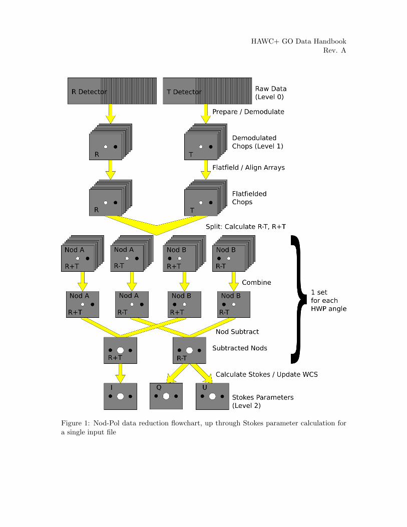
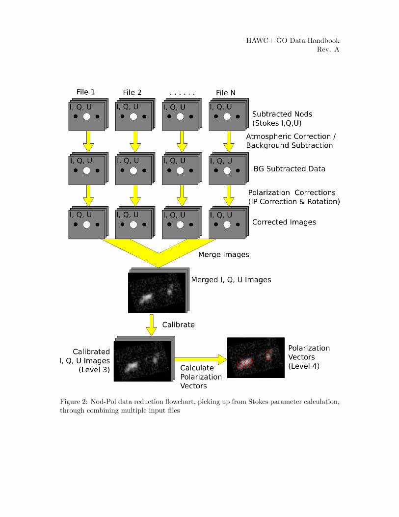
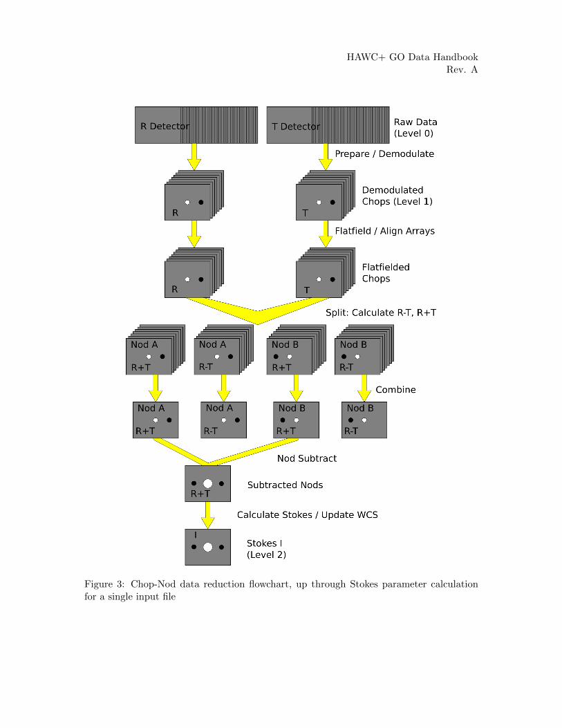
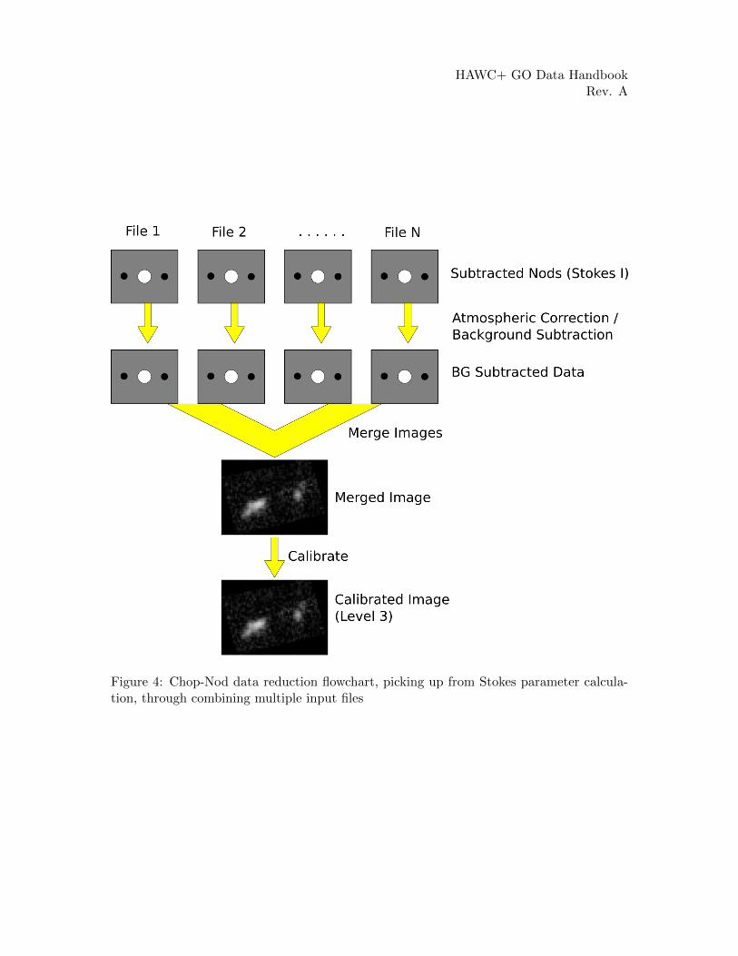
See the figures below for flow charts that illustrate the data reduction process for Nod-Poldata (Figures 1 and 2) and Chop-Nod data (Figures 3 and 4).

3.1.1 Prepare

The first step in the pipeline is to prepare the raw data for processing, by rearranging andregularizing the raw input data tables, and performing some initial calculations required


Figure 1: Nod-Pol data reduction flowchart, up through Stokes parameter calculation fora single input file


Figure 2: Nod-Pol data reduction flowchart, picking up from Stokes parameter calculation,through combining multiple input files


Figure 3: Chop-Nod data reduction flowchart, up through Stokes parameter calculationfor a single input file


Figure 4: Chop-Nod data reduction flowchart, picking up from Stokes parameter calcula-tion, through combining multiple input files


by subsequent steps.

The raw (Level 0) HAWC files contain all information in FITS binary table extensionslocated in two Header Data Unit (HDU) extensions. The raw file contains:

• Primary HDU: Contains the necessary FITS keywords in the header but no data. Itcontains all required keywords for SOFIA, plus all keywords required to reduce orcharacterize the various observing modes. Extra keywords (either from the SOFIAkeyword dictionary or otherwise) have been added for human parsing.

• CONFIGURATION HDU (EXTNAME = CONFIGURATION): HDU containingMCE (detector electronics) configuration data. This HDU is omitted for productsafter Level 1, so it is stored only in the raw and demodulated files. Nominally, it is thefirst HDU but users should use EXTNAME to identify the correct HDUs. Note, the“HIERARCH” keyword option and long strings are used in this HDU. All keywordnames are prefaced with “MCEn” where n=0,1,2,3. Only the header is used in thisHDU.

• TIMESTREAM Data HDU (EXTNAME = TIMESTREAM): Contains a binary ta-ble with data from all detectors, with one row for each time sample. The raw detectordata is stored in the column “SQ1Feedback”, in FITS (data-store) indices, i.e. 41rows and 128 columns. Columns 0-31 are for subarray R0, 32-63 for R1, 64-95 for T0and 96-127 for T1). Additional columns contain other important data and metadata,including time stamps, instrument encoder readings, chopper signals, and astrometrydata.

In order to begin processing the data, the pipeline first splits these input TIMESTREAMdata arrays into separate R and T tables. It will also compute nod and chop offset valuesfrom telescope data, and may also delete, rename, or replace some input columns in orderto format them as expected by later algorithms. The output data from this step has thesame HDU structure as the input data, but the detector data is now stored in the “RArray” and “T Array” fields, which have 41 rows and 64 columns each.

3.1.2 Demodulate

For both Chop-Nod and Nod-Pol instrument modes, data is taken in a two-point chopcycle. In order to combine the data from the high and low chop positions, the pipelinedemodulates the raw time stream with either a square or sine wave-form. Throughout thisstep, data for each of the R and T arrays are handled separately. The process is equivalentto identifying matched sets of chopped images and subtracting them.

During demodulation, a number of filtering steps are performed to identify good data.By default, the raw data is first filtered with a box high-pass filter with a time constant


of one over the chop frequency. Then, any data taken during telescope movement (line-of-sight rewinds, for example, or tracking errors) is flagged for removal. In square wavedemodulation, samples are then tagged as being in the high-chop state, low-chop state, orin between (not used). For each complete chop cycle within a single nod position at a singleHWP angle, the pipeline computes the average of the signal in the high-chop state andsubtracts it from the average of the signal in the low-chop state. Incomplete chop cyclesat the end of a nod or HWP position are discarded. The sine-wave demodulation proceedssimilarly, except that the data are weighted by a sine wave instead of being consideredeither purely high or purely low state.

During demodulation, the data is also corrected for the phase delay in the readout ofeach pixel, relative to the chopper signal. For square wave demodulation, the phase delaytime is multiplied by the sample frequency to calculate the delay in data samples for eachindividual pixel. The data is then shifted by that many samples before demodulating.For sine wave demodulation, the phase delay time is multiplied with 2π times the chopfrequency to get the phase shift of the demodulating wave-form in radians.

The result of the demodulation process is a chop-subtracted, time-averaged value for eachnod position, HWP angle, and array. The output is stored in a new FITS table, in theextension called DEMODULATED DATA, which replaces the TIMESTREAM data exten-sion. The CONFIGURATION extension is left unmodified.

3.1.3 Flat Correct

After demodulation, the pipeline corrects the data for pixel-to-pixel gain variations byapplying a flat field correction. Flat files for each filter band may provided to the pipelineby the instrument team, or they may be generated on the fly from internal calibrator files(CALMODE=INT CAL) taken alongside the science data. Either way, flat files containnormalized gains for the R and T array, so that they are corrected to the same level. Flatfiles also contain a bad pixel mask, with zero values indicating good pixels and any othervalue indicating a bad pixel. Pixels marked as bad are set to NaN in the gain data. Toapply the gain correction and mark bad pixels, the pipeline multiplies the R and T arraydata by the appropriate flat data. Since the T1 subarray is not available, all pixels in theright half of the T array are marked bad at this stage.

The output from this step contains FITS images that are propagated through the restof the pipeline steps. The R array data is stored as an image in the primary HDU; theT array data, R bad pixel mask, and T bad pixel mask are stored as images in exten-sions 1 (EXTNAME=“T ARRAY”), 2 (EXTNAME=“R BAD PIXEL MASK”), and 3(EXTNAME=“T BAD PIXEL MASK”), respectively. The DEMODULATED DATA ta-ble is attached unmodified as extension 4. The R and T array images are 3D cubes, with


dimension 64x41xNframe, where Nframe is the number of nod positions in the observation,times the number of HWP positions.

3.1.4 Align Arrays

In order to correctly pair R and T pixels for calculating polarization, and to spatially alignall subarrays, the pipeline must reorder the pixels in the raw images. The last row isremoved, R1 and T1 subarray images (columns 32-64) are rotated 180 degrees, and thenall images are inverted along the y-axis. Small shifts between the R0 and T0 and R1 andT1 subarrays may also be corrected for at this stage. The spatial gap between the 0 and 1subarrays is also recorded in the ALNGAPX and ALNGAPY FITS header keywords, butis not added to the image; it is accounted for in a later resampling of the image. Note thatall corrections applied in this step are integer shifts only; no interpolation is performed.The output images are 64x40xNframe.

3.1.5 Split Images

To prepare for combining nod positions and calculating Stokes parameters, the pipeline nextsplits the data into separate images for each nod position at each HWP angle, calculatesthe sum and difference of the R and T arrays, and merges the R and T array bad pixelmasks. The algorithm uses data from the DEMODULATED DATA table to distinguishthe high and low nod positions and the HWP angle. At this stage, any pixel for whichthere is a good pixel in R but not in T, or vice versa, is noted as a “widow pixel.” Inthe sum image (R+T), each widow pixel’s flux is multiplied by 2 to scale it to the correcttotal intensity. In the merged bad pixel mask, widow pixels are marked with the value 1(R only) or 2 (T only), so that later steps may handle them appropriately.

The output from this step contains a large number of FITS extensions: one DATA imageextension for each of R+T and R-T for each HWP angle and nod position, as well as aTABLE extension containing the demodulated data for each HWP angle and nod position,and a single merged BAD PIXEL MASK image. For a typical Nod-Pol observation with twonod positions and four HWP angles, there are 8 R+T images, 8 R-T images, 8 binary tables,and 1 bad pixel mask image, for 25 extensions total, including the primary HDU. Theoutput images, other than the bad pixel mask, are 3D cubes with dimension 64x40xNchop,where Nchop is the number of chop cycles at the given HWP angle.


3.1.6 Combine Images

The pipeline combines all chop cycles at a given nod position and HWP angle by computinga robust mean of all the frames in the R+T and R-T images. The robust mean is computedat each pixel using Chauvenet’s criterion, iteratively rejecting pixels more than 3σ fromthe mean value, by default. The associated standard deviation across the frames is storedas an error image in the output. The covariances between the pixels may also be calculatedand stored in the output, for later use in resampling the images.

The output from this step contains the same FITS extensions as in the previous step,with all images now reduced to 2D images with dimensions 64x40. In addition, there areERROR and COVAR image extensions for each nod position and HWP angle. Currently,covariances are not used in resampling, so they are not calculated for efficiency reasons;the COVAR images will contain NaN values only. In the example above, with two nodpositions and four HWP angles, there are now 57 total extensions, including the primaryHDU.

3.1.7 Subtract Beams

In this pipeline step, the sky nod positions (B beams) are subtracted from the source nodpositions (A beams) at each HWP angle and for each set of R+T and R-T, and the resultingflux is divided by two for normalization. The errors previously calculated in the combinestep are propagated accordingly. The output contains extensions for DATA, ERROR, andCOVAR images for each set, as well as a table of demodulated data for each HWP angle,and the bad pixel mask.

3.1.8 Compute Stokes

From the R+T and R-T data for each HWP angle, the pipeline now computes imagescorresponding to the Stokes I, Q, and U parameters for each pixel.

Stokes I is computed by averaging the R+T signal over all HWP angles:

I =1

N

N∑φ=1

(R+ T )(φ),

where N is the number of HWP angles and (R + T )(φ) is the summed R+T flux at theHWP angle φ. The associated uncertainty in I is generally propagated from the previouslycalculated errors for R+T, but may be inflated by the median of the standard deviation ofthe R+T values across the HWP angles if necessary.


In the most common case of four HWP angles at 0, 45, 22.5, and 67.5 degrees, Stokes Qand U are computed as:

Q =1

2[(R− T )(0)− (R− T )(45)]

U =1

2[(R− T )(22.5)− (R− T )(67.5)]

where (R− T )(φ) is the differential R-T flux at the HWP angle φ. Uncertainties in Q andU are propagated from the input error values on R-T.

The output from this step contains an extension for the flux, error, and covariance of eachStokes parameter, as well as the bad pixel mask and a table of the demodulated data,with columns from each of the HWP angles merged. The STOKES I flux image is inthe primary HDU. For Nod-Pol data, there will be 10 additional extensions (ERROR I,COVAR I, STOKES Q, ERROR Q, COVAR Q, STOKES U, ERROR U, COVAR U, BADPIXEL MASK, TABLE DATA). For Chop-Nod imaging, only Stokes I is calculated, sothere are 4 additional extensions (ERROR I, COVAR I, BAD PIXEL MASK, TABLEDATA).

3.1.9 Update WCS

To associate the pixels in the Stokes parameter image with sky coordinates, the pipelineuses FITS header keywords describing the telescope position to calculate the reference RAand Dec (CRVAL1/2), the pixel scale (CDELT1/2), and the rotation angle (CROTA2). Itmay also correct for small shifts in the pixel corresponding to the instrument boresight,depending on the filter used, by modifying the reference pixel (CRPIX1/2). These standardFITS world coordinate system (WCS) keywords are written to the header of the primaryHDU.

3.1.10 Correct for Atmospheric Opacity

In order to combine images taken under differing atmospheric conditions, the pipelinecorrects the flux in each individual file for the estimated atmospheric transmission duringthe observation, based on the altitude and zenith angle at the time when the observationwas obtained.

Atmospheric transmission values in each HAWC+ filter have been computed for a rangeof telescope elevations and observatory altitudes (corresponding to a range of overheadprecipitable water vapor values) using the ATRAN atmospheric modeling code, providedto the SOFIA program by Steve Lord. The ratio of the transmission at each altitude and


zenith angle, relative to that at the reference altitude (41,000 feet) and reference zenithangle (45 degrees), has been calculated for each filter and fit with a low-order polynomial.The ratio appropriate for the altitude and zenith angle of each observation is calculatedfrom the fit coefficients. The pipeline applies this relative opacity correction factor directlyto the flux in the Stokes I, Q, and U images, and propagates it into the corresponding errorimages.

3.1.11 Subtract Background

After chop and nod subtraction, some residual background noise may remain in the fluximages. After flat correction, some residual gain variation may remain as well. To removethese, the pipeline reads in all images in a reduction group, and then iteratively performsthe following steps:

• Smooth and combine the input Stokes I images

• Compare each Stokes I image (smoothed) to the combined map to determine anybackground offset or scaling

• Remove offset and scaling from input (unsmoothed) Stokes I images

The final determined offsets (a) and scales (b) for each file are applied to the flux F ′ foreach Stokes image as follows:

F ′I = (FI − a)/b

F ′Q = FQ/b

F ′U = FU/b

and are propagated into the associated error images appropriately.

3.1.12 Subtract Instrumental Polarization

The instrument and the telescope itself may introduce some foreground polarization to thedata which must be removed to determine the polarization from the astronomical source.The instrument team characterizes the introduced polarization in reduced Stokes (q = Q/Iand u = U/I) from the instrument and the telescope for each filter band. The combinedreduced Stokes parameters are calculated as

q′ = qi + qtcos(2E) + utsin(2E)

u′ = ui − qtsin(2E) + utcos(2E)


where qi and ui are the instrumental polarization parameters, qt and ut are the telescopepolarization parameters, and E is the average telescope elevation during the observation.The correction is then applied as

Q′ = Q− q′I

U ′ = U − u′I

and propagated to the associated error images as

σ′Q =√

(q′σI)2 + σ2Q.

σ′U =√

(u′σI)2 + σ2U .

The correction is expected to be good to within Q/I < 0.6% and U/I < 0.6%.

3.1.13 Rotate Polarization Coordinates

The Stokes Q and U parameters, as calculated so far, reflect polarization angles measuredin detector coordinates. After the foreground polarization is removed, the parameters maythen be rotated into sky coordinates. The pipeline calculates a relative rotation angle,α, that accounts for the vertical position angle of the instrument, the initial angle of thehalf-wave plate position, and an offset position that is different for each HAWC filter. Itapplies it to the Q and U images with a standard rotation matrix:(

Q′

U ′

)=

[cos(α) −sin(α)sin(α) cos(α)

](QU

).

Likewise, for the errors σ, the pipeline calculates(σ

′2Q

σ′2U

)=

[cos2(α) −sin2(α)sin2(α) cos2(α)

](σ2Qσ2U

),

takes the square root, and stores the result as the error images for Stokes Q and U.

3.1.14 Merge Images

All steps up until this point produce an output file for each input file taken at each telescopedither position, without changing the pixelization of the input data. To combine files takenat separate locations into a single map, the pipeline resamples the flux from each onto acommon grid, defined such that North is up and East is to the left. The WCS from eachinput file is used to determine the sky location of all the input pixels, then, for each pixel inthe output grid, the algorithm considers all input pixels within a given radius that are not


marked as bad pixels. It weights the input pixels by a Gaussian function of their distancefrom the grid point and, optionally, their associated errors and/or covariances. The valueat the output grid pixel is the weighted average of the input pixels within the consideredwindow.

The output from this step is a single FITS file, containing a flux and error image for eachof Stokes I, Q, and U. The dimensions of the output image may vary somewhat, dependingon the input parameters to the resampling algorithm, but typically the output pixel scaleis similar to the input scale. An image mask is also produced, which represents how manyinput pixels went into each output pixel. Because of the waiting scheme, the values in thismask are not integers. A data table containing demodulated data merged from all inputtables is also attached to the file.

3.1.15 Calibrate Flux

The pipeline now converts the flux units from instrumental counts to physical units ofJy/pixel. For each filter band, the instrument team determines a calibration factor inJy/pixel/counts appropriate to data that has been opacity-corrected to the reference zenithangle and altitude. This factor is directly applied to the flux in each of the Stokes I, Q, andU and associated error images. The overall calibration is expected to be good to withinabout 10%. See Section 4 for a more detailed description of the flux calibration processand the derivation of the calibration factors.

The output of this step is the final output from the pipeline for Chop-Nod imagingdata.

3.1.16 Compute Vectors

Using the Stokes I, Q, and U images, the pipeline now computes the polarization percentage(p) and angle (θ) and their associated errors (σ) in the standard way. For the polarizationangle θ in degrees:

θ =90

πarctan(

U

Q)

σθ =90

π(Q2 + U2)

√Q2σ2U + U2σ2Q.

The percent polarization (p) and its error are calculated from the reduced Stokes parame-ters q and u

q = Q/I

u = U/I


and their errorsσq =

√σ2Q + (Qσ2I )/I

σu =√σ2U + (Uσ2I )/I

asp = 100

√q2 + u2

σp =1

p

√q2σ2q + u2σ2u.

The debiased polarization percentage (p′)is also calculated, as:

p′ = 100√p2 − σ2p.

Each of the θ, p, and p′ maps and their error images are stored as separate extensions inthe output from this step, which is the final output from the pipeline for Nod-Pol data.This file will have 18 extensions, including the primary HDU, with extension names, types,and numbers as follows:

• STOKES I: primary HDU, image, extension 0

• ERROR I: image, extension 1

• STOKES Q: image, extension 2

• ERROR Q: image, extension 3

• STOKES U: image, extension 4

• ERROR U: image, extension 5

• IMAGE MASK: image, extension 6

• PERCENT POL: image, extension 7

• DEBIASED PERCENT POL: image, extension 8

• ERROR PERCENT POL: image, extension 9

• POL ANGLE: image, extension 10

• ROTATED POL ANGLE: image, extension 11

• ERROR POL ANGLE: image, extension 12

• POLARIZED FLUX: image, extension 13

• ERROR POLARIZED FLUX: image, extension 14


• MERGED DATA: table, extension 15

• POL DATA: table, extension 16

• FINAL POL DATA: table, extension 17

The final two extensions contain table representations of the polarization values for eachpixel, as an alternate representation of the θ, p, and p′ maps. The FINAL POL DATAtable is a subset of the POL DATA table, with data quality cuts applied.

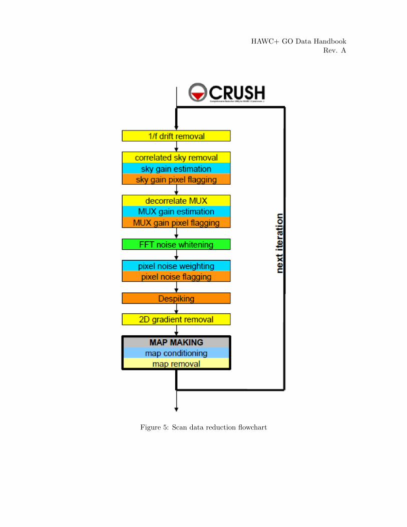
3.2 Scan Reduction Algorithms

This section covers the main algorithms used to reduce Scan mode data with CRUSH. Itis meant to give the reader an accurate, if incomplete, overview of the principal reductionprocess.

3.2.1 Signal Structure

CRUSH is based on the assumption that the measured data (Xct) for detector c, recordedat time t, is the superposition of various signal components and essential (not necessarilywhite) noise nct:

Xct = Dct + g(1),cC(1),t + ...+ g(n),cC(n),t +GcMxyct Sxy + nct

We can model the measured detector timestreams via a number of appropriate parame-ters, such as 1/f drifts (Dct), n correlated noise components (C(1),t...C(n),t) and channelresponses to these (gains, g(1),c...g(n),c), and the observed source structure (Sxy). We canderive statistically sound estimates (such as maximum-likelihood or robust estimates) forthese parameters based on the measurements themselves. As long as our model is repre-sentative of the physical processes that generate the signals, and sufficiently complete, ourderived parameters should be able to reproduce the measured data with the precision ofthe underlying limiting noise.

Below is a summary of the principal model parameters assumed by CRUSH, in gen-eral:

• Xct: The raw timestream of channel c, measured at time t.

• Dct: The 1/f drift value of channel c at time t.

• g(1),c...g(n),c: Channel c gain (response) to correlated signals (for modes 1 throughn).

• C(1),t...C(n),t: Correlated signals (for modes 1 through n) at time t.


Figure 5: Scan data reduction flowchart


• Gc: The point source gain of channel c

• Mxyct : Scanning pattern, mapping a sky position x, y into a sample of channel c at

time t.

• Sxy: Actual 2D source flux at position x, y.

• nct: Essential limiting noise in channel c at time t.

3.2.2 Sequential Incremental Modeling and Iterations

The approach of CRUSH is to solve for each term separately, and sequentially, rather thantrying to do a brute-force matrix inversion in a single step. Such inversions are not practicalfor several reasons, anyway: (1) because they require a-priori knowledge of all gains andweights (covariance matrix) with great precision, (2) because they require bad data tobe identified prior to inversion, (3) because degeneracies are not handled in a controlled /controllable way, (4) because linear inversions do not handle non-linearities with ease (suchas solving for both gains and signals when these form a product), (5) because of the need toinclude spectral filtering, typically, and (6) because matrix inversions are computationallycostly.

Sequential modeling works on the assumption that each term can be considered indepen-dently from one another. To a large degree this is granted as many of the signals producemore or less orthogonal imprints in the data (e.g. you cannot easily mistake correlatedsky response seen by all channels with a per-channel DC offset). As such, from the pointof view of each term, the other terms represent but an increased level of noise. As theterms all take turns in being estimated (usually from bright to faint) this model confusion“noise” goes away, especially with iterations.

Even if the terms are not perfectly orthogonal to one another, and have degenerate fluxcomponents, the sequential approach handles this naturally. Degenerate fluxes between apair of terms will tend to end up in the term that is estimated first. Thus, the orderingof the estimation sequence provides a control on handling degeneracies in a simple andintuitive manner.

A practical trick for efficient implementation is to replace the raw timestream with theunmodeled residuals Xct → Rct, and let modeling steps produce incremental updates tothe model parameters. Every time a model parameter is updated, its incremental imprint isremoved from the residual timestream (a process we shall refer to a synchronization).

With each iteration, the incremental changes to the parameters become more insignificant,and the residual will approach the limiting noise of the measurement.


3.2.3 DC Offset and 1/f Drift Removal

For 1/f drifts, consider only the term:

Rct ≈ δDcτ

where δDcτ is the 1/f channel drift value for t between τ and τ+T , for a 1/f time window ofT samples. That is, we simply assume that the residuals are dominated by an unmodeled1/f drift increment δDcτ . Note that detector DC offsets can be treated as a special casewith τ = 0, and T equal to the number of detector samples in the analysis.

We can construct a χ2 measure, as:

χ2 =

t=τ+T∑c,t=τ

wct(Rct − δDct)2

where wct = σ−2ct is the proper noise-weight associated with each datum. CRUSH further-more assumes that the noise weight of every sample wct can be separated into the productof a channel weight wc and a time weight wt, i.e. wct = wc ·wt. This assumption is identicalto that of separable noise (σct = σc · σt). Then, by setting the χ2 minimizing condition∂χ2/∂(δDct) = 0, we arrive at the maximum-likelihood incremental update:

δDcτ =

τ+T∑t=τ

wtRct

τ+T∑t=τ

wt

Note, that each sample (Rct) contributes a fraction:

pct = wt/

τ+T∑t=τ

wt

to the estimate of the single parameter δDcτ . In other words, this is how much thatparameter is dependent on each data point. Above all, pct is a fair measure of the fractionaldegrees of freedom lost from each datum, due to modeling of the 1/f drifts. We will usethis information later, when estimating proper noise weights.

Note, also, that we may replace the maximum-likelihood estimate for the drift parameterwith any other statistically sound estimate (such as a weighted median), and it will notreally change the dependence, as we are still measuring the same quantity, from the samedata, as with the maximum-likelihood estimate. Therefore, the dependence calculationremains a valid and fair estimate of the degrees of freedom lost, regardless of what statisticalestimator is used.


The removal of 1/f drifts must be mirrored in the correlated signals also if gain solutions areto be accurate. Finally, following the removal of drifts, CRUSH will check the timestreamsfor inconsistencies. For example, HAWC data is prone to discontinuous jumps in flux levels.CRUSH will search the timestream for flux jumps, and flag or fix jump-related artifacts asnecessary.

3.2.4 Correlated Noise Removal and Gain Estimation

For the correlated noise (mode i), we shall consider only the term with the incrementalsignal parameter update:

Rct = g(i),cδC(i),t + ...

Initially, we can assume C(i),t as well as g(i),c = 1, if better values of the gain are notindependently known at the start. Accordingly, the χ2 becomes:

χ2 =∑c

wct(Rct − g(i),cδC(i),t)2.

Setting the χ2 minimizing condition with respect to δC(i),t yields:

δC(i),t =

∑cwcg(i),cRct∑cwcg2(i),c

.

The dependence of this parameter on Rct is:

pct = wcg2(i),c/

∑c

wcg2(i),c

After we update C(i) (the correlated noise model for mode i) for all frames t, we can updatethe gain response as well in an analogous way, if desired. This time, consider the residualsdue to the unmodeled gain increment:

Rct = δg(i),cC(i),t + ...

andχ2 =

∑t

wct(Rct − δg(i),cC(i),t)2

Minimizing it with respect to δg(i),c yields:

δg(i),c =

∑twtC(i),tRct∑twtC2

(i),t


which has a parameter dependence:

pct = wtC2(i),t/

∑t

wtC2(i),t

Because the signal Ct and gain gc are a product in our model, scaling Ct by some factorX, while dividing gc by the same factor will leave the product intact. Therefore, oursolutions for Ct and gc are not unique. To remove this inherent degeneracy, it is practicalto enforce a normalizing condition on the gains, such that the mean gain µ(gc) = 1,by construct. CRUSH uses a robust mean measure for gain normalization to producereasonable comparisons under various pathologies, such as when most gains are zero, orwhen a few gains are very large compared to the others.

Once again, the maximum-likelihood estimate shown here can be replaced by other statis-tical measures (such as a weighted median), without changing the essence.

3.2.5 Noise Weighting

Once we model out the dominant signal components, such that the residuals are startingto approach a reasonable level of noise, we can turn our attention to determining propernoise weights. In its simplest form, we can determine the weights based on the meanobserved variance of the residuals, normalized by the remaining degrees of freedom in thedata:

wc = ηcN(t),c − Pc∑twtR2

ct

where N(t),c is the number of unflagged data points (time samples) for channel c, and Pc isthe total number of parameters derived from channel c. The scalar value ηc is the overallspectral filter pass correction for channel c (see section 3.2.7), which is 1 if the data wasnot spectrally filtered, and 0 if the data was maximally filtered (i.e. all information isremoved). Thus typical ηc values will range between 0 and 1 for rejection filters, or can begreater than 1 for enhancing filters. We determine time-dependent weights as:

wt =N(c),t − Pt∑cwcR2

ct

Similar to the above, here N(c),t is the number of unflagged channel samples in frame t,while Pt is the total number of parameters derived from frame t. Once again, it is practicalto enforce a normalizing condition of setting the mean time weight to unity, i.e. µ(wt) = 1.This way, the channel weights wc have natural physical weight units, corresponding towc = 1/σ2c .


The total number of parameters derived from each channel, and frame, are simply the sum,over all model parameters m, of all the parameter dependencies pct we calculated for them.That is,

Pc =∑m

∑t

p(m),ct

andPt =

∑m

∑c

p(m),ct

Getting these lost-degrees-of-freedom measures right is critical for the stability of the so-lutions in an iterated framework. Even slight biases in pct can grow exponentially withiterations, leading to divergent solutions, which may manifest as over-flagging or as extrememapping artifacts.

Of course, one may estimate weights in different ways, such as based on the median absolutedeviation (robust weights), or based on the deviation of differences between nearby samples(differential weights). As they all behave the same for white noise, there is really nosignificant difference between them. CRUSH does, optionally, offer those different (butcomparable) methods of weight estimation.

3.2.6 Despiking

After deriving fair noise weights, we can try to identify outliers in the data (glitches andspikes) and flag them for further analysis. Despiking is a standard procedure that need notbe discussed here in detail. CRUSH offers a few variants of the basic method, dependingon whether it looks for absolute deviations, differential deviations between nearby data, orspikes at different resolutions (multires) at once.

3.2.7 Spectral Conditioning

Ideally, detectors would have featureless white noise spectra (at least after the 1/f noise istreated by the drift removal). In practice, that is rarely the case. Spectral features are badbecause (a) they produce mapping features/artifacts (such as “striping”), and because (b)they introduce a covariant noise term between map points that is not easily representedby the output. It is therefore desirable to “whiten” the residual noise whenever possible,to mitigate both these effects.

Noise whitening starts with measuring the effective noise spectrum in a temporal window,significantly shorter than the integration on which it is measured. In CRUSH, the tempo-ral window is designed to match the 1/f stability timescale T chosen for the drift removal,since the drift removal will wipe out all features on longer timescales. With the use of such


a spectral window, we may derive a lower-resolution averaged power-spectrum for eachchannel. CRUSH then identifies the white noise level, either as the mean (RMS) scalaramplitude over a specified range of frequencies, or automatically, over an appropriate fre-quency range occupied by the point-source signal as a result of the scanning motion.

Then, CRUSH will look for significant outliers in each spectral bin, above a specified level(and optimally below a critical level too), and create a real-valued spectral filter profile φcffor each channel c and frequency bin f to correct these deviations.

There are other filters that can be applied also, such as notch filters, or a motion filterto reject responses synchronous to the dominant telescope motion. In the end, every oneof these filters is represented by an appropriate scalar filter profile φcf , so the discussionremains unchanged.

Once a filter profile is determined, we apply the filter by first calculating a rejected sig-nal:

%ct = F−1[(1− φcf )Rcf ]

where Rcf is the Fourier transform of Rct, using the weighting function provided by wt,and F−1 denotes the inverse Fourier Transform from the spectral domain back into thetimestream. The rejected signals are removed from the residuals as:

Rct → Rct − %ct

The overall filter pass ηc for channel c, can be calculated as:

ηc =

∑f

φ2cf

Nf

where Nf is the number of spectral bins in the profile φcf . The above is simply a measure ofthe white-noise power fraction retained by the filter, which according to Parseval’s theorem,is the same as the power fraction retained in the timestream, or the scaling of the observednoise variances as a result of filtering.

3.2.8 Map Making

The mapping algorithm of CRUSH implements a nearest-pixel method, whereby each datapoint is mapped entirely into the map pixel that falls nearest to the given detector channelc, at a given time t. Distributing the flux to neighboring pixels would constitute smoothing,and as such, it is better to smooth maps explicitly by a desired amount as a later processingstep. Here,

δSxy =

∑ctM ctxywcwtκcGcRct∑

ctM ctxywcwtκ2

cG2c


where M ctxy associates each sample c, t uniquely with a map pixel x, y, and is effectively

the transpose of the mapping function defined earlier. κc is the point-source filtering (pass)fraction of the pipeline. It can be thought of as a single scalar version of the transferfunction. Its purpose is to measure how isolated point-source peaks respond to the variousreduction steps, and correct for it. When done correctly, point source peaks will alwaysstay perfectly cross-calibrated between different reductions, regardless of what reductionsteps were used in each case. More generally, a reasonable quality of cross-calibration (towithin 10%) extends to compact and slightly extended sources (typically up to about halfof the field-of-view (FoV) in size). While corrections for more extended structures (≥ FoV)are possible to a certain degree, they come at the price of steeply increasing noise at thelarger scales.

The map-making algorithm should skip over any data that is unsuitable for quality map-making (such as too-fast scanning that may smear a source). For formal treatment, we canjust assume that Mxy

ct = 0 for any troublesome data.

Calculating the precise dependence of each map point Sxy on the timestream data Rctis computationally costly to the extreme. Instead, CRUSH gets by with the approxima-tion:

pct ≈ Nxy ·wt∑twt· wcκ2

cGc∑cwcκ2

cG2c

This approximation is good as long as most map points are covered with a representativecollection of pixels, and as long as the pixel sensitivities are more or less uniformly dis-tributed over the field of view. So far, the inexact nature of this approximation has notproduced divergent behavior with any of the dozen or more instruments that CRUSH isbeing used with. Its inaccuracy is of no grave concern as a result.

We can also calculate the flux uncertainty in the map σxy at each point x, y as:

σ2xy = 1/∑ct

M ctxywcwtκ2

cG2c

Source models are first derived from each input scan separately. These may be despikedand filtered, if necessary, before added to the global increment with an appropriate noiseweight (based on the observed map noise) if source weighting is desired.

Once the global increment is complete, we can add it to the prior source model Sr(0)xy and

subject it to further conditioning, especially in the intermediate iterations. Conditioningoperations may include smoothing, spatial filtering, redundancy flagging, noise or exposureclipping, signal-to-noise blanking, or explicit source masking. Once the model is processed

into a finalized S′xy, we synchronize the incremental change δS′xy = S′xy − Sr(0)xy to the

residuals:Rct → Rct −Mxy

ct (δGcSr(0)xy +GcδS

′xy)


Note, again, that δS′xy 6= δSxy. That is, the incremental change in the conditioned sourcemodel is not the same as the raw increment derived above. Also, since the source gainsGc may have changed since the last source model update, we must also re-synchronize the

prior source model S(0)xy with the incremental source gain changes δGc (first term inside the

brackets).

Typically, CRUSH operates under the assumption that the point-source gains Gc of thedetectors are closely related to the observed sky-noise gains gc derived from the correlatednoise for all channels. Specifically, CRUSH treats the point-source gains as the prod-uct:

Gc = εcgcgse−τ

where εc is the point-source coupling efficiency. It measures the ratio of point-source gainsto sky-noise gains (or extended source gains). Generally, CRUSH will assume εc = 1, unlessthese values are measured and loaded during the scan validation sequence. Optionally,CRUSH can also derive εc from the observed response to a source structure, provided thescan pattern is sufficient to move significant source flux over all detectors. The source gainsalso include a correction for atmospheric attenuation, for an optical depth τ , in-band andin the line of sight. Finally, a gain term gs for each input scan may be used as a calibrationscaling/correction on a per-scan basis.

3.2.9 Point-Source Flux Corrections

We mentioned point-source corrections in the section above; here, we explain how theseare calculated. First, consider drift removal. Its effect on point source fluxes is a reductionby a factor:

κD,c ≈ 1− τpntT

In terms of the 1/f drift removal time constant T and the typical point-source crossingtime τpnt. Clearly, the effect of 1/f drift removal is smaller the faster one scans across thesource, and becomes negligible when τpnt T .

The effect of correlated-noise removal, over some group of channels of mode i, is a littlemore complex. It is calculated as:

κ(i),c = 1− 1

N(i),t(P(i),c +

∑k

ΩckP(i),k)

where Ωck is the overlap between channels c and k. That is, Ωck is the fraction of the pointsource peak measured by channel c when the source is centered on channel k. N(i),t is thenumber of correlated noise-samples that have been derived for the given mode (usually the


same as the number of time samples in the analysis). The correlated model’s dependenceon channel c is:

P(i),c =∑t

p(i),ct

Finally, the point-source filter correction due to spectral filtering is calculated based on theaverage point-source spectrum produced by the scanning. Gaussian source profiles withspatial spread σx ≈ FWHM/2.35 produce a typical temporal spread σt ≈ σx/v, in termsof the mean scanning speed v. In frequency space, this translates to a Gaussian frequencyspread of σf = (2πσt)

−1, and thus a point-source frequency profile of:

Ψf ≈ e−f2/(2σ2

f )

More generally, Ψf may be complex-valued (asymmetric beam). Accordingly, the point-source filter correction due to filtering with φf is generally:

κφ,c ≈

∑f

Re(φfΨfφf )∑f

Re(Ψf )

The compound point source filtering effect from m model components is the product ofthe individual model corrections, i.e.:

κc =∏m

κ(m),c

This concludes the discussion of the principal reduction algorithms of CRUSH for HAWCScan mode data. For more information, see section 3.3.

3.2.10 CRUSH output

Since the CRUSH algorithms are iterative, there are no well-defined intermediate productsthat may be written to disk. For Scan mode data, the pipeline takes as input a set of rawLevel 0 HAWC FITS files, described in section 3.1.1, and writes as output a single FITS filecontaining an image of the source map, and several other extensions. The primary HDU inthe output file contains the flux image (EXTNAME = SIGNAL) in units of Jy/pixel. Thefirst extension (EXTNAME = EXPOSURE) contains an image of the nominal exposuretime in seconds at each point in the map. The second extension (EXTNAME = NOISE)holds the error image corresponding to the flux map, and the third extension (EXTNAME= S/N) is the signal-to-noise ratio of the flux to the error image. The fourth and furtherextensions contain binary tables of data, one for each input scan.


3.3 Other Resources

For more information on the code or algorithms used in the HAWC DRP or the CRUSHpipelines, see the following documents:

DRP:

• Far-infrared polarimetry analysis: Hildebrand et. al. 2000 PASP, 112, 1215

• DRP infrastructure and image viewer: Berthoud, M. 2013 ADASS XXII, 475, 193

CRUSH:

• CRUSH paper: Kovacs, A. 2008, Proc. SPIE, 7020, 45

• CRUSH thesis: Kovacs, A. 2006, PhD Thesis, Caltech

• Online documentation: http://www.submm.caltech.edu/~sharc/crush

4 Flux Calibration

As part of the reduction process, the pipeline generates fully calibrated products, in whicheach pixel is assigned a physical flux in Jy by first correcting the instrumental value at thatpixel for telluric absorption (see Sec. 3.1.10) and then dividing the result by a calibrationfactor. The calibration factors are derived for each HAWC+ filter from observations ofcalibrator targets. Since stars are fairly faint at the HAWC wavelengths, the calibrationtargets consist of planets and/or moons for which good theoretical models of their spectraexist. The process of calibrating HAWC+ images is very similar to that used for calibratingFORCAST images (see Herter et al. 2013), with the difference resulting from the fact thatthe HAWC+ detectors are bolometers, sensitive to energy rather than photons.

4.1 Reduction Steps

The calibration is carried out in several steps. The first step consists of measuring thephotometry of all the standards for a specific mission or flight series, after the images havebeen corrected for the atmospheric transmission relative to that for a reference altitude andzenith angle (see section 3.1.10 which describes the corrections for atmospheric opacity).A photometric aperture radius of 12−15 pixels is used for this measurement. The telluric-corrected photometry of the standard source is related to the measured photometry of thesource via

N std,corrcts = N std

cts

(RrefλRstdλ

)

http://iopscience.iop.org/article/10.1086/316613

http://adsabs.harvard.edu/abs/2013ASPC..475..193B

http://adsabs.harvard.edu/abs/2008SPIE.7020E..45K

http://adsabs.harvard.edu/abs/2006PhDT........28K

http://www.submm.caltech.edu/~sharc/crush


where Ncts is the instrumental flux in counts/s and the ratio Rrefλ /Rstdλ accounts for thedifferences in system response (i.e., atmospheric transmission) between the conditions forthe actual observations and those for a reference altitude of 41000 feet and a telescopeelevation of 45 deg. Similarly, for the science target we have

Nobj,corrcts = N std

obj

(Rrefλ

Robjλ

).

Calibration factors (in counts/s/Jy) for each filter are then derived from the measuredphotometry (in counts/s) and the known fluxes of the standards (in Jy) in each filter.The predicted fluxes in each filter were computed by multiplying a model standard sourcespectrum (generally, planets and moons for which reliable mid-infrared spectra exist) bythe overall filter + instrument + telescope + atmosphere (at the reference altitude andzenith angle) response curve and integrating over the filter passband to compute the meanflux in the band,

⟨F stdν

⟩. The adopted filter throughput curves are those provided by the

vendor. The instrument throughput is calculated by multiplying the transmission curvesand emissivity values of the entrance window, the foreoptics, and internal optics. Thetelescope throughput value is assumed to be constant (85%) across the entire HAWC+wavelength range.

The flux of the science target is then given by

Fnom,objν (λref ) =Nobj,corrcts

C

where Nobj,corrcts is the telluric-corrected count rate in counts/s detected from the source, C

is the calibration factor (counts/s/Jy), and Fnom,objν (λref ) is the flux in Jy of a nominal,‘flat spectrum’ source (for which νFν = constant) at a reference wavelength λref . We takeλref to be the mean wavelength 〈λ〉 of the filter. The calibration factor, C is computedfrom the flux and instrumental photometry of the standard via

C =N std,corrcts

Fnom,stdν

(λref ) =N std,corrcts

〈F stdν 〉λ2pivλrefλ′

with an uncertainty given by(σCC

)2=

(σNstd

cts

N stdcts

)2

+

(σ〈F stdν 〉

〈F stdν 〉

)2

.

Here, 〈F stdν 〉 is the mean flux over the passband, λpiv is the pivot wavelength of the filter,given by

λ2piv =

∫Sdλ∫Sλ2dλ


and λ′ is a characteristic wavelength given by

λ′ =

∫Sdλ∫Sλdλ

.

Here, S is the total system throughput. The calibration factor thus defined refers to anominal, flat spectrum source at the reference wavelength.

The calibration factors derived from each standard for each filter are then averaged. Afterall calibration factors are derived for a flight series, the final step involves examining thecalibration values and ensuring that the values are consistent. Outlier values may comefrom bad observations of a standard star; these values are removed to produce a robustaverage of the calibration factor across the flight series. The resulting average values arethen used to calibrate the observations of the science targets.

4.2 Color Corrections

An observer often wishes to determine the true flux of an object at the reference wavelength,F objν (λref ), rather than the flux of an equivalent flat spectrum source. To do this, we definea color correction K such that

K =Fnom,objν (λref )

F objν (λref )

where Fnom,objν (λref ) is the flux density obtained from a measurement on the final pipeline-reduced data product. One must divide the measured value by K to obtain the true fluxdensity. In terms of the wavelengths defined above, we have

K =λrefλ

′

λ2piv

〈F objν 〉F objν (λref )

.

The color corrections K can then be computed for an assumed input spectral shape. Formost filters and spectral shapes, the color corrections are small (< 10%). Tables listingK values for various input source spectral shapes and filter wavelengths are available fromthe SOFIA website.

5 Data Products

5.1 File names

Output files from the HAWC pipeline are named according to the convention:


FILENAME = F[flight] HA [mode] [aorid] [spectel] [type] [fn1[-fn2]].fits

where flight is the SOFIA flight number, HA indicates the instrument (HAWC+), and modeis either IMA for imaging observations, POL for polarization observations, or CAL for di-agnostic data. The aorid indicates the SOFIA program and observation number, spectelindicates the filter/band and the HWP setting. The type is a three-letter identifier for thepipeline product type, and fn1 and fn2 are the first and last raw file numbers that were com-bined to produce the output product. For example, a polarization vector data product withAOR-ID 81 0131 04 derived from files 5 to 6 of flight 295, taken in Band A with HWP in theA position would have the filename F0295 HA POL 81013104 HAWAHWPA VEC 005-006.fits. See the tables below for a list of all possible values for the three-letter producttype.

5.2 Data format

Most HAWC data is stored in FITS files, conforming to the FITS standard (Pence et al.2010). Each FITS file contains a primary Header Data Unit (HDU) which may containthe most appropriate image data for that particular data reduction level. Most files haveadditional data stored in HDU image or table extensions. All keywords describing the fileare in the header of the primary HDU. Each HDU has its own header and is identified bythe EXTNAME header keyword. The algorithm descriptions, above, give more informationabout the content of each extension.

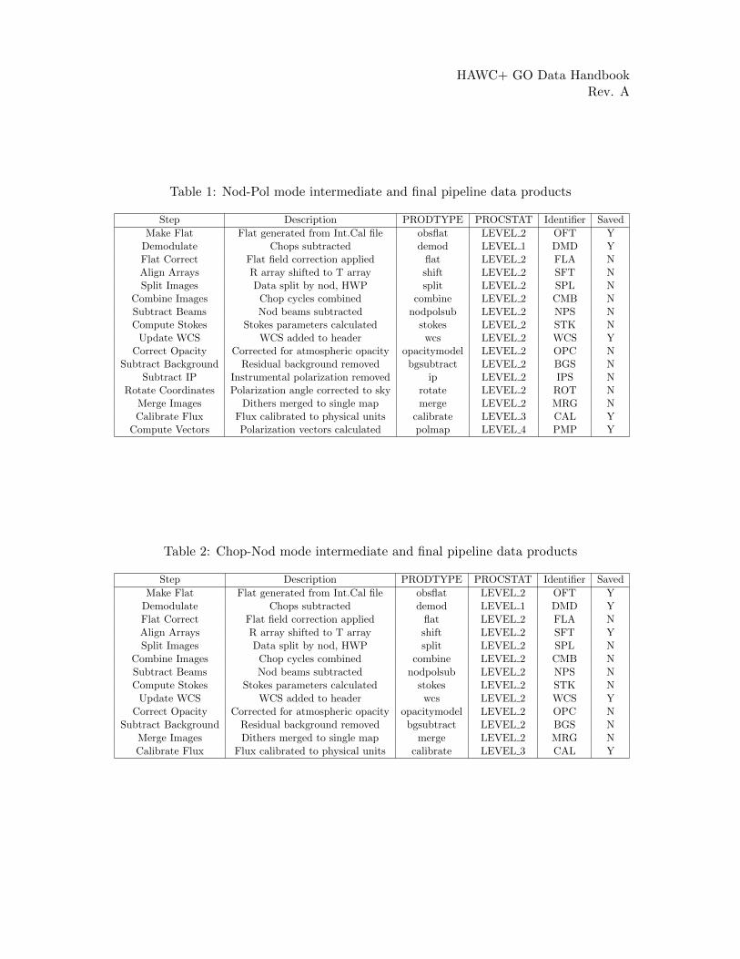
5.3 Pipeline products

The following tables list all intermediate and final products that may be generated by theHAWC pipeline, in the order in which they are produced for each mode. The product typeis stored in the primary header, under the keyword PRODTYPE. By default, for Nod-Polmode, the shift, wcs, calibrate, and polvec products are saved. For Chop-Nod mode, theshift, wcs, merge, and calibrate products are saved. For Scan mode, only the crush productis produced or saved.

6 References

Herter et al. 2013, PASP, 125, 1393


Table 1: Nod-Pol mode intermediate and final pipeline data products

Step Description PRODTYPE PROCSTAT Identifier Saved

Make Flat Flat generated from Int.Cal file obsflat LEVEL 2 OFT YDemodulate Chops subtracted demod LEVEL 1 DMD YFlat Correct Flat field correction applied flat LEVEL 2 FLA NAlign Arrays R array shifted to T array shift LEVEL 2 SFT NSplit Images Data split by nod, HWP split LEVEL 2 SPL N

Combine Images Chop cycles combined combine LEVEL 2 CMB NSubtract Beams Nod beams subtracted nodpolsub LEVEL 2 NPS NCompute Stokes Stokes parameters calculated stokes LEVEL 2 STK N

Update WCS WCS added to header wcs LEVEL 2 WCS YCorrect Opacity Corrected for atmospheric opacity opacitymodel LEVEL 2 OPC N

Subtract Background Residual background removed bgsubtract LEVEL 2 BGS NSubtract IP Instrumental polarization removed ip LEVEL 2 IPS N

Rotate Coordinates Polarization angle corrected to sky rotate LEVEL 2 ROT NMerge Images Dithers merged to single map merge LEVEL 2 MRG NCalibrate Flux Flux calibrated to physical units calibrate LEVEL 3 CAL Y

Compute Vectors Polarization vectors calculated polmap LEVEL 4 PMP Y

Table 2: Chop-Nod mode intermediate and final pipeline data products


Make Flat Flat generated from Int.Cal file obsflat LEVEL 2 OFT YDemodulate Chops subtracted demod LEVEL 1 DMD YFlat Correct Flat field correction applied flat LEVEL 2 FLA NAlign Arrays R array shifted to T array shift LEVEL 2 SFT YSplit Images Data split by nod, HWP split LEVEL 2 SPL N

Combine Images Chop cycles combined combine LEVEL 2 CMB NSubtract Beams Nod beams subtracted nodpolsub LEVEL 2 NPS NCompute Stokes Stokes parameters calculated stokes LEVEL 2 STK N

Update WCS WCS added to header wcs LEVEL 2 WCS YCorrect Opacity Corrected for atmospheric opacity opacitymodel LEVEL 2 OPC N

Subtract Background Residual background removed bgsubtract LEVEL 2 BGS NMerge Images Dithers merged to single map merge LEVEL 2 MRG NCalibrate Flux Flux calibrated to physical units calibrate LEVEL 3 CAL Y


Table 3: Scan mode final pipeline data product


CRUSH Source model derived iteratively with CRUSH crush LEVEL 3 CRH Y

guest observer handbook for hawc+ data products · hawc+ go data handbook rev. a guest observer...

Documents