guidance, control and trajectory tracking of small fixed wing unmanned aerial vehicles (uav's)...
TRANSCRIPT

Guidance, Control and Trajectory Tracking of Small Fixed Wing
Unmanned Aerial Vehicles (UAV’s)
A THESIS IN MECHATRONICS
Presented to the faculty of the American University of Sharjah
College of Engineering
in partial fulfillment of
the requirements for the degree of
MASTER OF SCIENCE
by
AMER A. KH. AL-RADAIDEH
B.S. 2006
Sharjah, UAE
April 2009

c©2009
AMER A. KH. AL-RADAIDEH
ALL RIGHTS RESERVED

Guidance, Control and Trajectory Tracking of Small Fixed WingUnmanned Aerial Vehicles (UAV’s)
Amer A.KH.Al-Radaideh, Candidate for Master of Science in MechatronicsEngineering
American University of Sharjah, 2009
ABSTRACT
Unmanned Aerial Vehicles (UAV’s) have gained increasing considerations dueto their low cost and increased autonomy. A large number of applications in themilitary and civilian fields. The present work considers a low level flight control algo-rithms (auto-pilot) to improve the guidance, path following and trajectory trackingcapabilities of the low speed fixed wing AUS-UAV. In addition, this investigationaims the development and building of fully functioning test-bed UAV platform. Thetest-bed includes an enhanced hardware in the loop simulation ”HILS” system tofacilitate the development and evaluation of the ability of the flight control systems(FCS) of the AUS-UAV to follow prescribed trajectories.
At the end of this thesis, the AUS-UAV was modelled using ground basednumerical modelling for the aerodynamic coefficients in the early phases. Then, theaerodynamic coefficients estimation was enhanced using flight test based identifica-tion. The engine and actuator were also identified.
Furthermore, a trajectory tracking algorithm was designed, implemented andevaluated using HILS. The avionics unit was also designed, calibrated and tested.Finally, flight test were conducted using Krestal autopilot to experiment with flighttesting and compare the performance with our avionics unit HILS results.
iii
Contents
Abstract iii
List of Figures vi
List of Tables x
Nomenclature xii
Acknowledgements xvi
1 Introduction 1
1.1 Unmanned Aerial Vehicles(UAVs) . . . . . . . . . . . . . . . . . . . . 1
1.1.1 Predator . . . . . . . . . . . . . . . . . . . . . . . . . . . . . . 2
1.1.2 Hermes . . . . . . . . . . . . . . . . . . . . . . . . . . . . . . 3
1.1.3 Aerosonde . . . . . . . . . . . . . . . . . . . . . . . . . . . . . 3
1.2 UAV History . . . . . . . . . . . . . . . . . . . . . . . . . . . . . . . 4
1.3 UAV Missions and Applications . . . . . . . . . . . . . . . . . . . . . 6
1.4 Guidance and control Background . . . . . . . . . . . . . . . . . . . . 7
1.5 Previous research on UAVs at AUS . . . . . . . . . . . . . . . . . . . 9
1.6 Thesis objectives and contribution . . . . . . . . . . . . . . . . . . . . 11
1.7 Thesis outline . . . . . . . . . . . . . . . . . . . . . . . . . . . . . . . 12
2 ARF60 AUS-UAV Nonlinear Model and Dynamics Equations 14
2.1 UAV Coordinate Frames and Axis System Definition . . . . . . . . . 14
2.1.1 Inertial Frame . . . . . . . . . . . . . . . . . . . . . . . . . . . 14
2.1.2 Body Frame . . . . . . . . . . . . . . . . . . . . . . . . . . . . 14
2.1.3 Stability Frame . . . . . . . . . . . . . . . . . . . . . . . . . . 15
2.1.4 Wind Frame . . . . . . . . . . . . . . . . . . . . . . . . . . . . 16
2.2 UAV Aerodynamic Control Surfaces . . . . . . . . . . . . . . . . . . . 17
2.3 UAV Equations of Motion . . . . . . . . . . . . . . . . . . . . . . . . 20
2.3.1 UAV Forces and Moments . . . . . . . . . . . . . . . . . . . . 20
2.3.2 UAV Orientation and Position . . . . . . . . . . . . . . . . . . 23
2.4 Aerodynamic coefficients for forces and moments . . . . . . . . . . . . 24
2.4.1 Aerodynamic Forces . . . . . . . . . . . . . . . . . . . . . . . 24
2.4.2 Aerodynamic Moments . . . . . . . . . . . . . . . . . . . . . . 25
2.5 Implementation of the ARF60 AUS-UAV Nonlinear Model in Simulink 25
iv

3 ARF60 AUS-UAV Modeling and System Identifications 27
3.1 Introduction . . . . . . . . . . . . . . . . . . . . . . . . . . . . . . . . 27
3.2 Overview of UAV System ID and literature Review . . . . . . . . . . 28
3.3 System ID steps . . . . . . . . . . . . . . . . . . . . . . . . . . . . . . 30
3.4 Aircraft System ID . . . . . . . . . . . . . . . . . . . . . . . . . . . . 31
3.4.1 Aerodynamic Numerical modeling . . . . . . . . . . . . . . . . 31
3.4.2 Flight Tests Based System ID . . . . . . . . . . . . . . . . . . 33
3.5 OS 61FX Engine and its Propeller System ID . . . . . . . . . . . . . 40
3.6 Actuator System ID . . . . . . . . . . . . . . . . . . . . . . . . . . . 42
4 ARF60 AUS-UAV Aircraft Natural Motion, Controller Design andSimulation 45
4.1 Aircraft Linear Model . . . . . . . . . . . . . . . . . . . . . . . . . . 45
4.1.1 ARF60 UAV Longitudinal Model . . . . . . . . . . . . . . . . 45
4.1.2 ARF60 UAV Lateral Model . . . . . . . . . . . . . . . . . . . 47
4.2 ARF60 UAV Autopilot design using Successive Loop Closure (SLC) . 50
4.2.1 Autopilot Overview . . . . . . . . . . . . . . . . . . . . . . . . 50
4.2.2 Longitudinal Autopilot . . . . . . . . . . . . . . . . . . . . . . 55
4.2.3 Lateral Autopilot . . . . . . . . . . . . . . . . . . . . . . . . . 62
4.2.4 Trajectory Tracker(Shortest Flight Algorithm in 3D) . . . . . 66
5 Control and Hardware Implementation 71
5.1 Signals, Hardware and Software . . . . . . . . . . . . . . . . . . . . . 72
5.1.1 Control Signals . . . . . . . . . . . . . . . . . . . . . . . . . . 72
5.1.2 Control Hardware . . . . . . . . . . . . . . . . . . . . . . . . . 72
5.2 Avionics . . . . . . . . . . . . . . . . . . . . . . . . . . . . . . . . . . 74
5.2.1 Flight Controller Computer (MPC555 Microcontroller) . . . . 74
5.2.2 INS/GPS Unit . . . . . . . . . . . . . . . . . . . . . . . . . . 75
5.2.3 Battery and Power Distribution Board . . . . . . . . . . . . . 77
5.3 Ground Station Design . . . . . . . . . . . . . . . . . . . . . . . . . . 77
5.3.1 Ground Station GUI . . . . . . . . . . . . . . . . . . . . . . . 78
5.4 Summary . . . . . . . . . . . . . . . . . . . . . . . . . . . . . . . . . 82
6 Hardware in the loop Simulation (HILS) 84
6.1 Hardware in the Loop Simulation Development . . . . . . . . . . . . 85
6.1.1 ARF60 UAV 6-DOF model simulator . . . . . . . . . . . . . . 85
6.1.2 R/C transmitter . . . . . . . . . . . . . . . . . . . . . . . . . 86
6.1.3 Data communication and synchronization . . . . . . . . . . . 87
6.1.4 HILS Summary . . . . . . . . . . . . . . . . . . . . . . . . . . 88
6.2 Hardware in the loop Simulation Results . . . . . . . . . . . . . . . . 89
6.2.1 HILS Autopilot Results . . . . . . . . . . . . . . . . . . . . . . 89
6.2.2 HILS Trajectory Tracking Results . . . . . . . . . . . . . . . . 89
v

7 Flight Tests Results and Autopilot Tuning 95
7.1 Kestrel Autopilot Overview . . . . . . . . . . . . . . . . . . . . . . . 95
7.1.1 Mounting Kestrel Autopilot on the ARF60 UAV . . . . . . . . 96
7.1.2 Flight Testing Using Kestrel Autopilot . . . . . . . . . . . . . 101
8 Thesis Summary and Future Work 119
8.1 Summary and Contributions . . . . . . . . . . . . . . . . . . . . . . . 119
8.1.1 Avionics Unit Development . . . . . . . . . . . . . . . . . . . 119
8.1.2 System Identification and Aircraft Nonlinear Modelling . . . . 119
8.1.3 Developing Hardware in The Loop Simulation . . . . . . . . . 119
8.1.4 Implementing SLC Based Autopilot and Trajectory TrackingUsing Simulink Embedded Model-based Design . . . . . . . . 119
8.1.5 Developing Common Ground Station for UxV’s in AUS . . . . 120
8.1.6 Flight Testing . . . . . . . . . . . . . . . . . . . . . . . . . . . 120
8.2 Future Work . . . . . . . . . . . . . . . . . . . . . . . . . . . . . . . . 120
8.2.1 Ground Station Enhancement . . . . . . . . . . . . . . . . . . 120
8.2.2 Nonlinear Autopilot and Trajectory Tracking Enhancement . . 120
8.2.3 Nonlinear System Identification . . . . . . . . . . . . . . . . . 120
A Geometry, Aerodynamic, and other Aircraft Design information 121
A.1 Aircraft Geometry Definitions . . . . . . . . . . . . . . . . . . . . . . 121
A.1.1 Wingspan . . . . . . . . . . . . . . . . . . . . . . . . . . . . . 121
A.1.2 Mean Aerodynamic Chord (MAC) . . . . . . . . . . . . . . . 121
A.1.3 Aspect ratio (AR) . . . . . . . . . . . . . . . . . . . . . . . . 122
B Hardware and Softwares Used in This Thesis 123
B.1 Hardware . . . . . . . . . . . . . . . . . . . . . . . . . . . . . . . . . 123
B.1.1 OS FS120 Engine . . . . . . . . . . . . . . . . . . . . . . . . . 123
B.1.2 MIDG II INS/GPS . . . . . . . . . . . . . . . . . . . . . . . . 123
B.1.3 MPX4115A Absolute Pressure Sensor . . . . . . . . . . . . . . 125
B.1.4 1INCHGBASIC Differential Pressure Sensor . . . . . . . . . . 126
C Engine and Actuators System Identification 127
C.1 Engine System ID . . . . . . . . . . . . . . . . . . . . . . . . . . . . . 127
C.1.1 The Engine and its Propeller Modeling . . . . . . . . . . . . . 127
C.2 Actuator System ID . . . . . . . . . . . . . . . . . . . . . . . . . . . 128
References 134
vi
List of Figures
1.1 Predator-UAV. . . . . . . . . . . . . . . . . . . . . . . . . . . . . . . 3
1.2 Hermes 450 UAV. . . . . . . . . . . . . . . . . . . . . . . . . . . . . . 4
1.3 Aerosonde-UAV. . . . . . . . . . . . . . . . . . . . . . . . . . . . . . 5
1.4 RPioneer, first commissioned UAV. . . . . . . . . . . . . . . . . . . . 6
1.5 AUS Avionics Unit constructed in (Hadi, 2005) . . . . . . . . . . . . 10
1.6 The HILS Setup designed in (Hassan, 2006) . . . . . . . . . . . . . . 10
1.7 The Ground Station Built in (Hassan, 2006) . . . . . . . . . . . . . . 11
1.8 UAV System Architecture . . . . . . . . . . . . . . . . . . . . . . . . 12
2.1 Inertial Axis Definition . . . . . . . . . . . . . . . . . . . . . . . . . . 15
2.2 Body Axis Definition . . . . . . . . . . . . . . . . . . . . . . . . . . . 15
2.3 Stability Axis Definition . . . . . . . . . . . . . . . . . . . . . . . . . 16
2.4 Wind Axis Definition . . . . . . . . . . . . . . . . . . . . . . . . . . . 16
2.5 Control Surface Deflection . . . . . . . . . . . . . . . . . . . . . . . . 17
2.6 Aileron Control Surface . . . . . . . . . . . . . . . . . . . . . . . . . . 18
2.7 Elevator Control Surface . . . . . . . . . . . . . . . . . . . . . . . . . 19
2.8 Rudder Control Surface . . . . . . . . . . . . . . . . . . . . . . . . . 19
2.9 ARF60 UAV Simulink Model general Structure . . . . . . . . . . . . 26
3.1 UAV components dynamics and control . . . . . . . . . . . . . . . . . 29
3.2 System Identification Steps . . . . . . . . . . . . . . . . . . . . . . . . 31
3.3 CG location Experiment top . . . . . . . . . . . . . . . . . . . . . . . 32
3.4 CG location Experiment . . . . . . . . . . . . . . . . . . . . . . . . . 32
3.5 Construction of System identification for the ARF60 UAV . . . . . . 35
3.6 ARF60 Actuators deflections during the system identification test . . 35
3.7 ARF60 Angular Rates during the system identification test . . . . . . 36
3.8 ARF60 Accelerations during the system identification test . . . . . . 36
3.9 ARF60 Attitudes during the system identification test . . . . . . . . . 37
3.10 ARF60 Velocities during the system identification test . . . . . . . . 37
3.11 ARF60 Position during the system identification test . . . . . . . . . 38
3.12 ARF60 Air Data during the system identification test . . . . . . . . . 38
3.13 The OS 61FX RPM measured output for the validation data set, to-gether with the output from the ARX, ARMAX, OE and BJ modelswhen simulated with the input sequence from the validation data set 42
3.14 The OS 61FX thrust measured output for the validation data set, to-gether with the output from the ARX, ARMAX, OE and BJ modelswhen simulated with the input sequence from the validation data set 43
vii
3.15 Thrust measured output together with the output from the BJ modelwhen simulated with the input PRBS . . . . . . . . . . . . . . . . . . 43
3.16 Actuator Identifcation Setup . . . . . . . . . . . . . . . . . . . . . . . 44
4.1 Poles Locations for the Longitudinal Model . . . . . . . . . . . . . . . 47
4.2 Impulse Response for the Longitudinal Model . . . . . . . . . . . . . 48
4.3 Poles Locations for the Lateral Model . . . . . . . . . . . . . . . . . . 49
4.4 Aircraft in a Steady Banked Turn . . . . . . . . . . . . . . . . . . . . 53
4.5 SISO Design Task,Root Locus Graphical Tuning Window, AnalysisPlots and Compensator Parameters Tuning Editor. . . . . . . . . . . 56
4.6 Pitch Rate Damping Block Diagram . . . . . . . . . . . . . . . . . . 57
4.7 Pitch Rate Damping Root Locus . . . . . . . . . . . . . . . . . . . . 58
4.8 Pitch attitude hold using elevator Block Diagram . . . . . . . . . . . 59
4.9 Pitch attitude hold using elevator step response . . . . . . . . . . . . 60
4.10 Altitude hold using commanded pitch Block Diagram . . . . . . . . . 60
4.11 Altitude hold using commanded pitch loop step response . . . . . . . 61
4.12 Airspeed hold using throttle Block Diagram . . . . . . . . . . . . . . 62
4.13 Airspeed hold using throttle step response . . . . . . . . . . . . . . . 62
4.14 ARF60 Longitudinal Autopilot Block Diagram . . . . . . . . . . . . . 63
4.15 Roll Rate Damping Block Diagram . . . . . . . . . . . . . . . . . . . 63
4.16 Roll Attitude Hold Block Diagram . . . . . . . . . . . . . . . . . . . 64
4.17 Dutch Roll Damper Block Diagram . . . . . . . . . . . . . . . . . . . 65
4.18 ARF60 Lateral Autopilot Block Diagram . . . . . . . . . . . . . . . . 65
4.19 Path taken by the UAV When Entering a Curve using Feedback Guid-ance . . . . . . . . . . . . . . . . . . . . . . . . . . . . . . . . . . . . 66
4.20 Extension of the Feedback Guidance Strategy - Bidirectional . . . . . 67
4.21 ARF60 Autopilot and Trajectory Tracker System Block Diagram . . . 68
4.22 Four waypoints navigation results . . . . . . . . . . . . . . . . . . . . 69
4.23 Four waypoints navigation Map 2D . . . . . . . . . . . . . . . . . . . 70
4.24 Four waypoints navigation plot 3D . . . . . . . . . . . . . . . . . . . 70
5.1 AUS Avionics and Ground station Block Diagram . . . . . . . . . . . 71
5.2 AUS Avionics Unit. . . . . . . . . . . . . . . . . . . . . . . . . . . . . 74
5.3 MIDG II:Inertial Navigation System (INS) with Global PositioningSystem (GPS) . . . . . . . . . . . . . . . . . . . . . . . . . . . . . . . 75
5.4 Block Diagram of Avionics Power Distribution . . . . . . . . . . . . . 77
5.5 Autopilot Panel-Ground Station . . . . . . . . . . . . . . . . . . . . . 78
5.6 Desired Commands Panel-Ground Station . . . . . . . . . . . . . . . 79
5.7 Actuators Monitoring Panel-Ground Station . . . . . . . . . . . . . . 79
5.8 States Monitoring Panel-Ground Station . . . . . . . . . . . . . . . . 80
5.9 Ground Station Map . . . . . . . . . . . . . . . . . . . . . . . . . . . 81
5.10 Ground Station Map Settings . . . . . . . . . . . . . . . . . . . . . . 81
5.11 PID Loops Parameters-Ground Station . . . . . . . . . . . . . . . . . 82
5.12 Data Log Panel-Ground Station . . . . . . . . . . . . . . . . . . . . . 82
viii

5.13 Communication Settings Panel-Ground Station . . . . . . . . . . . . 83
6.1 Hardware-in-the-loop (HIL) simulation Setup . . . . . . . . . . . . . . 85
6.2 Hardware-in-the-loop (HIL) simulation environment . . . . . . . . . . 87
6.3 HILS Autopilot Test 1 -Attitudes . . . . . . . . . . . . . . . . . . . . 90
6.4 HILS Autopilot Test 2 - States Results . . . . . . . . . . . . . . . . . 90
6.5 2WP Navigation-2D . . . . . . . . . . . . . . . . . . . . . . . . . . . 91
6.6 2WP Navigation-3D . . . . . . . . . . . . . . . . . . . . . . . . . . . 91
6.7 2WP Navigation-Map . . . . . . . . . . . . . . . . . . . . . . . . . . . 92
6.8 2WP Navigation-Attitudes . . . . . . . . . . . . . . . . . . . . . . . . 92
6.9 4WP Navigation (Hourglass Shape)-2D . . . . . . . . . . . . . . . . . 93
6.10 4WP Navigation (Hourglass Shape)-3D . . . . . . . . . . . . . . . . . 93
6.11 4WP Navigation (Hourglass Shape)-Map . . . . . . . . . . . . . . . . 94
6.12 4WP Navigation (Hourglass Shape)-Attitudes . . . . . . . . . . . . . 94
7.1 Kestrel Autopilot . . . . . . . . . . . . . . . . . . . . . . . . . . . . . 96
7.2 Kestrel Autopilot Diagram . . . . . . . . . . . . . . . . . . . . . . . . 96
7.3 Kestrel Autopilot Block Diagram . . . . . . . . . . . . . . . . . . . . 97
7.4 Kestrel Autopilot with spacers . . . . . . . . . . . . . . . . . . . . . . 97
7.5 Kestrel Autopilot isolation from inside . . . . . . . . . . . . . . . . . 98
7.6 Kestrel Autopilot isolation from outside . . . . . . . . . . . . . . . . . 98
7.7 Kestrel Autopilot inside the Aluminume box . . . . . . . . . . . . . . 99
7.8 GPS Location on the aircraft . . . . . . . . . . . . . . . . . . . . . . 99
7.9 RF Antenna Location on the Aircraft . . . . . . . . . . . . . . . . . . 100
7.10 Pitot Static Tube Location on the Aircraft . . . . . . . . . . . . . . . 100
7.11 Pitot Static Tube Location on the Aircraft . . . . . . . . . . . . . . . 101
7.12 Crashed test (1) . . . . . . . . . . . . . . . . . . . . . . . . . . . . . . 102
7.13 Crashed test (2) . . . . . . . . . . . . . . . . . . . . . . . . . . . . . . 102
7.14 Roll Hold Test1 . . . . . . . . . . . . . . . . . . . . . . . . . . . . . . 104
7.15 Roll Hold Test1 Error Analysis . . . . . . . . . . . . . . . . . . . . . 104
7.16 Roll Hold Test1 Map . . . . . . . . . . . . . . . . . . . . . . . . . . . 105
7.17 Roll Hold Test2 . . . . . . . . . . . . . . . . . . . . . . . . . . . . . . 105
7.18 Roll Hold Test2 Error Analysis . . . . . . . . . . . . . . . . . . . . . 106
7.19 Roll Hold Test2 Map . . . . . . . . . . . . . . . . . . . . . . . . . . . 106
7.20 Pitch Hold Test . . . . . . . . . . . . . . . . . . . . . . . . . . . . . . 107
7.21 Airspeed Hold Test . . . . . . . . . . . . . . . . . . . . . . . . . . . . 107
7.22 150m Loiter Test . . . . . . . . . . . . . . . . . . . . . . . . . . . . . 109
7.23 Error Analysis for the Altitude from the 150m Loiter Test . . . . . . 110
7.24 Error Analysis for the Pitch from the 150m Loiter Test . . . . . . . . 110
7.25 Error Analysis for the Roll from the 150m Loiter Test . . . . . . . . . 111
7.26 150m Loiter Test Map . . . . . . . . . . . . . . . . . . . . . . . . . . 111
7.27 Square Pattern . . . . . . . . . . . . . . . . . . . . . . . . . . . . . . 112
7.28 Four Waypoints Square Trajectory Test . . . . . . . . . . . . . . . . . 112
ix
7.29 Four Waypoints Square Trajectory Test Analysis . . . . . . . . . . . . 113
7.30 Four Waypoints Square 3D Trajectory . . . . . . . . . . . . . . . . . 113
7.31 Four Laps:Four Waypoints Square 2D Trajectory . . . . . . . . . . . 114
7.32 Four Laps:Four Waypoints Square 3D Trajectory . . . . . . . . . . . 114
7.33 Four Laps:Four Waypoints Square 3D Trajectory Map . . . . . . . . . 115
7.34 Hourglass Pattern . . . . . . . . . . . . . . . . . . . . . . . . . . . . . 115
7.35 Four Waypoints Hourglass Trajectory Test . . . . . . . . . . . . . . . 116
7.36 Four Waypoints Hourglass Trajectory Test Analysis . . . . . . . . . . 116
7.37 Four Waypoints Hourglass 3D Trajectory . . . . . . . . . . . . . . . . 117
7.38 Three Laps:Four Waypoints Hourglass 3D Trajectory . . . . . . . . . 117
7.39 Three Laps:Three Waypoints Hourglass 3D Trajectory Map . . . . . . 118
B.1 OS FS120 Engine . . . . . . . . . . . . . . . . . . . . . . . . . . . . . 123
B.2 MIDG II:Inertial Navigation System (INS) with Global PositioningSystem (GPS) . . . . . . . . . . . . . . . . . . . . . . . . . . . . . . . 124
B.3 MMPX4115A Absolute Pressure Sensor . . . . . . . . . . . . . . . . . 125
C.1 Load Cell Calibration Plot . . . . . . . . . . . . . . . . . . . . . . . . 129
C.2 Engine Identification Setup . . . . . . . . . . . . . . . . . . . . . . . . 130
C.3 PRBS PWM Signal Generation using dSpace Toolbox Blocks . . . . . 130
C.4 RPM Measurement using dSpace Toolbox Blocks . . . . . . . . . . . 131
C.5 Thrust Measurement using dSpace Toolbox Blocks . . . . . . . . . . 131
C.6 Actuator Identifcation Setup . . . . . . . . . . . . . . . . . . . . . . . 131
C.7 Aileron actuator response with the doblets input . . . . . . . . . . . . 132
C.8 Aileron Actuator Identifcation Results for Doublets inputs . . . . . . 132
C.9 Aileron actuator response with the PRBS input . . . . . . . . . . . . 133
C.10 Aileron Actuator Identifcation Results for PRBS inputs . . . . . . . . 133
x
List of Tables
3.1 ARF60 measured geometric parameters - input to the MATLAB script 33
3.2 Stability derivatives of the ARF60 UAV (All units per radian) . . . . 34
3.3 Identified Stability derivatives of the ARF60 UAV (All units per ra-dian) using System ID algorithm . . . . . . . . . . . . . . . . . . . . 41
3.4 OS 61FX Engine RPM System ID Results . . . . . . . . . . . . . . . 41
3.5 OS 61FX Engine Thrust System ID Results . . . . . . . . . . . . . . 42
4.1 Pole locations, natural frequencies and periods for the longitudinalmodes. . . . . . . . . . . . . . . . . . . . . . . . . . . . . . . . . . . . 47
4.2 Pole locations, natural frequencies and periods for the lateral modes. 49
4.3 Pitch attitude hold using elevator loop gains . . . . . . . . . . . . . . 59
4.4 Altitude hold using commanded pitch loop gains . . . . . . . . . . . . 61
4.5 Airspeed hold using throttle loop gains . . . . . . . . . . . . . . . . . 62
4.6 Dutch Roll Damper loop gains . . . . . . . . . . . . . . . . . . . . . . 65
5.1 MIDG II Specifications . . . . . . . . . . . . . . . . . . . . . . . . . . 76
5.2 Cost, Mass and Power Consumption . . . . . . . . . . . . . . . . . . 83
7.1 Calibration data . . . . . . . . . . . . . . . . . . . . . . . . . . . . . . 102
7.2 Stability Augmentation System (SAS) gains . . . . . . . . . . . . . . 103
7.3 Inner Attitude Hold Loops gains . . . . . . . . . . . . . . . . . . . . . 108
7.4 Outer Airspeed Hold PID Loops Gains . . . . . . . . . . . . . . . . . 108
7.5 Outer Altitude Hold PID Loops Gains . . . . . . . . . . . . . . . . . 108
B.1 S FS120 Engine Specifications . . . . . . . . . . . . . . . . . . . . . . 124
C.1 Load cell calibration data . . . . . . . . . . . . . . . . . . . . . . . . 129
xi

Nomenclature
Axis System (Reference Frames), Angles and Transformations
i Inertial reference frameB Body reference frameFi(OiXiYiZi) Inertial axis systemFB(OBXBYBZB) Body axis systemFS(OSXSYSZS) Stability FrameFW (OWXWYWZW ) Wind Frameh Altitudeϕ Latitudeλ Longitudeφ Roll angleθ Pitch angleψ Yaw angleα Angle of Attack (AOA)β Angle of Side Slip (AOS)
Earth Quantities (WGS-84)
gn Normal gravitational acceleration (ϕ = 45o)a Equatorial radius of the Earth (semimajor axis) = 6378137.000 mb polar radius of the Earth (semiminor axis) = 6356752.3142 mΩ Earth turn rate with respect to i frame = 7.292116× 10⁻⁵ rad/sg l Local gravity column matrixf Flattening (ellipticity) = 1/298.257223563 (0.00335281066474)e Major eccentricity of Earth = 0.0818191908426µ Earth’s gravitational constant = 3986005× 108m3/s2
M Mass of Earth (including the atmosphere) = 5.9733328× 1024 Kg
System Identifications
ARX Autoregressive with exogenous inputs modelARMAX Autoregressive moving average model with exogenous inputs modelOE Output ErrorBJ Box-Jenkins
Stability Derivatives
CL Zero alpha liftCLα Alpha derivativeCLαt
Alpha derivative for the tail
xii

CLαvAlpha derivative for the vertical tail
CLδePitch control (elevator) derivative
CLαAlpha-dot derivative
CLq Pitch rate derivativeCD Minimum dragCDδe
Pitch control (elevator) derivativeCDδa
Roll control (aileron) derivativeCDδr
Yaw control (rudder) derivativeCYβ
Sideslip derivativeCYδa
Roll control derivativeCYδr
Yaw control derivativeCYp Roll rate derivativeCYrr Yaw rate derivativeCm Zero alpha pitchCmα Alpha derivativeCmδe
Pitch control derivativeCmα
Alpha dot derivativeCmq Pitch rate derivativeClβ Sideslip derivativeClδa
Roll control derivativeClδr
Yaw control derivativeClp Roll rate derivativeClr Yaw rate derivativeCnβ
Sideslip derivativeCnδa
Roll control derivativeCnδr
Yaw control derivativeCnp Roll rate derivativeCnr Yaw rate derivative
Static Quantities
AR aspect ratiob wing span (i.e., tip to tip)c wing chord (varies along span)c mean aerodynamic chord (mac)S wing area totalλ taper ratio (tip chord/root chord)Λ leading-edge sweep angleJx Moment of inertia in the x-axisJy Moment of inertia in the y-axisJz Moment of inertia in the z-axisJxz Moment of inertia in the xz-plane
Dynamic Quantities
D DragL Lift
xiii

`w Rolling momentmw Pitching momentnw Yawing momentVn Normal gravitational acceleration (ϕ = 45o)V n
e Kinematic velocity expressed in n frameωb
nb Angular rate of b frame relative to n frame expressed in b frameωn
en Angular rate of n frame relative to e frame expressed in n frameωb
ib Angular rate of b frame relative to n frame expressed in b framef e Specific force in b frame
f b Specific force in n framevN , vE, vD The north, east and down components of V n
e
fN , fE, fD The north, east and down components of f ne
Vair The true UAV airspeedu X-axis velocity in the body framev Y-axis velocity in the body framew Z-axis velocity in the body framep Roll rateq Pitch rater Yaw rateCX Drag force aerodynamic coefficientCY Side force aerodynamic coefficientCZ Lift force aerodynamic coefficientC` X-axis aerodynamic moment coefficientCm Y-axis aerodynamic moment coefficientCn Z-axis aerodynamic moment coefficient
Subscripts
j, k, l Indexes for high speed computer cycle (j-cycle), moderate computerspeed cycle (k-cycle) and low computer speed cycle (l-cycle) respec-tively
N,E,D North, East and Down components of n frame vector
Abbreviations
ARF Almost Ready to FlyCOTS Cost-Of-The-ShelfCR Confidence RegionDCM Direction Cosine MAtrixDGPS Differential Global Positioning SystemDOF Degrees of FreedomECEF Earth-Centered Earth-FixedGPS Global Positioning SystemIMU Inertial Measurement UnitINS Inertial Navigation SystemKF Kalman FilterNED North-East-Down
xiv

UAV Unmanned Aerial VehiclePRBS Pseud Random Binary Sequence
xv

Acknowledgements
This MSc Thesis has only been possible with the help and support of some people Iwould like to thank very much.
First of all, I would like to sincerely thank my advisor Prof.Dr.Mohammad-AmeenAl Jarrah for his support during this thesis, for the guidance, support and for alwaysbelieving in me and pushing me for more.
It is difficult to overstate my appreciation to Dr.Ali Jhemi, who gave me a lot of hisvaluable time and provided me with a lot of support. And I am deeply grateful tomy colleagues Elvanto Ikhsan, Tri Hardimasyar and Guntur Supriyadi. I cant forgetall the days that we spent in flight testing.
To all the colleagues in the Mechatronics Program, Hossein Sadjadi, Hussein Sahli,Laith Sahawneh, Mohammed Assadi, Amal Khattab, Tariq Abu-Hashim, YasmeenAbu-Kheil, Ali Ghazi, Mohammed Saleh, Khaled Al-Suwaidi, Oubada Al-Dabbas,Hazaa Al-Abdouli, Hamad Al-Kotbi, Faisal Al-Kabi, Behrooz Mozafferi, Ihab Abu-Younis, Younes Al-Younes and Mahmoud Ghaith. The best friends ever. Thank Youall.
I am also very grateful to all my professors in AUS for teaching me such fascinatingtopics during those two years. I would not have brought this project very far withoutsuch a previous knowledge.
Thanks go to the ILL people at AUS-Library, for your non-ending support.
Finally, I would like to thank all my friends in AUS, and particularly those who helpedme enjoying those first two years in UAE.
To my parents, brothers and sister, whom my words can’t describe.
To Knowledge.
xvi
Chapter 1
Introduction
Unmanned Aerial Vehicles (UAVs) research and development is a growing area as their
cost and reliability is improving. However, significant development is needed in order
to get a reliable autonomous system capable of performing all types of maneuvers with
reasonable performance and stability. Advanced control algorithms are usually non-
linear methods of feedback control implemented in the Digital Flight Control System
(DFCS) of the UAV, or what is usually called the autopilot. The autopilot consists
of several components that are integrated together along with a tailored embedded
software to perform a specific task. Autonomous UAV’s operation is improving con-
tiguously from advances in other technologies like sensor fusion, propulsion systems,
navigation aids and single-chip embedded system. Advance control technology, em-
bedded systems, and MEMS technology made autonomous systems feasible and cost
effective (Jung, 2001). The availability and ease of use of this kind of technologies
made it relatively cost effective and affordable to develop UAVs’ advanced control
systems. In this chapter a brief introduction to UAVs, what they are, and what they
do, as well as their history and previous work done will be presented. Finally, we will
state the thesis’ objectives and contribution.
1.1 Unmanned Aerial Vehicles(UAVs)
UAV is Unmanned Aerial Vehicle that is controlled autonomously by an integrated
system called the Autopilot. In the old days, the autopilot was built using ana-
log circuits that form several PID (Proportional Integral Derivative)loops to provide
aircraft stability. Nowadays, microcontrollers with embedded software are used in
modern control of a UAV. Microcontrollers are the brain of the autopilot, they read
the signals from all onboard sensors, like inertial sensors and air data sensors, and
then they process the data according to the control algorithm and command the actu-
ator accordingly. The initial design of autopilots served as a Stability Augmentation
1.1 Unmanned Aerial Vehicles(UAVs) 2
System (SAS) that provides proper flight stability of a marginally stable or unstable
aircrafts. But in UAVs the autopilot takes full control over the aircraft. With a spe-
cific mission programmed in the microcontroller, UAVs can be fully autonomous. But
most UAVs nowadays can also be remotely controlled in case of any emergency. UAVs
vary in size, cost, mission, and endurance. They can be from a several inches micro
size UAV that perform very short missions to over one hundred feet UAV that has high
endurance and high range communication capabilities like High Altitude Long En-
durance (HALE) (www.gruntsmilitary.com). UAVs have several features that make
them attractive. It’s not only their capability of flying autonomously and perform-
ing specific missions, but also because they are relatively inexpensive compared to
manned aircrafts. Using UAVs in dangerous missions behind enemy lines will also
protect the lives of human pilots. A new breed of UAVs is the UCAVs (Unmanned
Combat Aerial Vehicle) (Pike, 2005) which are designed to address a variety of the
most dangerous missions due to their high maneuverability and endurance. These
vehicles are usually stealthy and used for suppression of enemy air defenses, persis-
tent surveillance, reconnaissance and precision strike (www.gruntsmilitary.com). An
example of these UCAVs is the Boeing X-45A UCAV (Pike, 2005). Below are several
examples of UAVs and some details about each one of them.
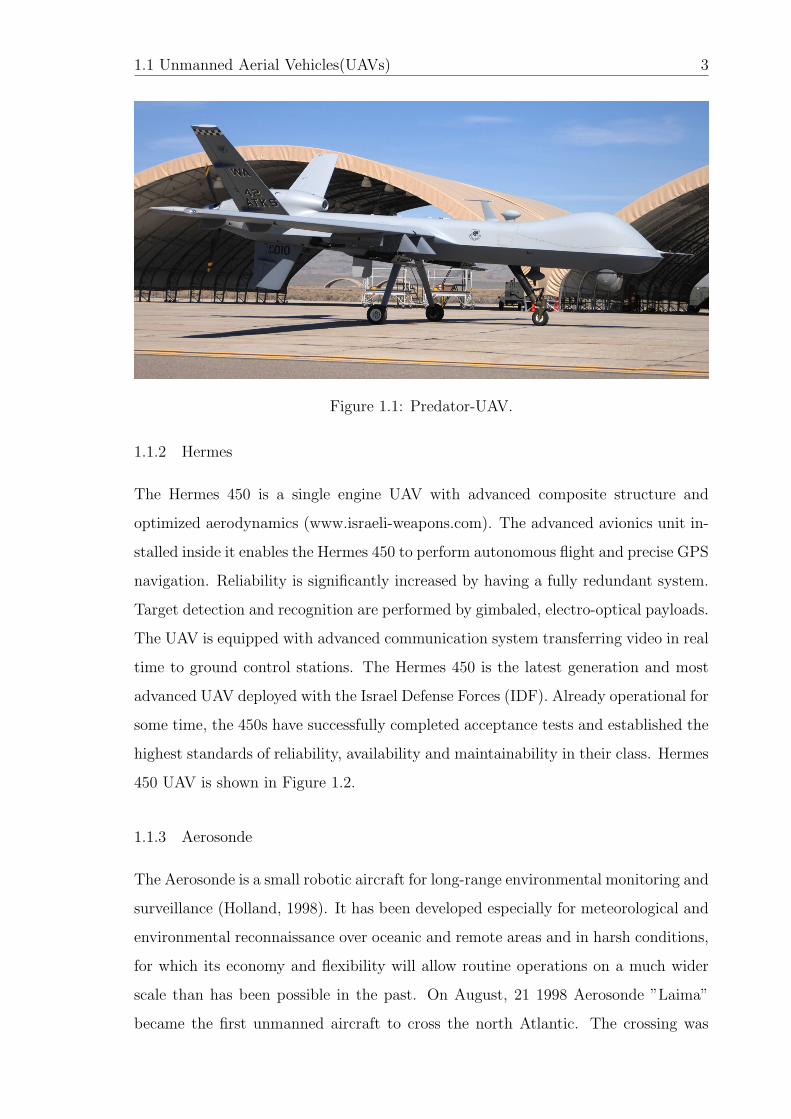
1.1.1 Predator
The Predator was the first tactical UAV with significant participation in the U.S. Air
Force (www.gruntsmilitary.com). With a range of up to 500 miles, and endurance
capabilities exceeding 20 hours, the Predator was designed with the capability to
provide near real time imagery intelligence to the theater through use of infrared
sensors along with payloads capable of penetrating adverse weather. The Predator
is flown by Air Force pilots from a remote facility with the air vehicle controlled by
line-of-sight satellite relay data links. During 1995 and 1996, the Predator was flown
in Albania in support of relief operations as well as follow-on operations in Bosnia
supporting Operation Deny Flight. Predator UAV is shown in Figure 1.1.
1.1 Unmanned Aerial Vehicles(UAVs) 3
Figure 1.1: Predator-UAV.
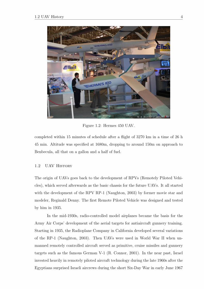
1.1.2 Hermes
The Hermes 450 is a single engine UAV with advanced composite structure and
optimized aerodynamics (www.israeli-weapons.com). The advanced avionics unit in-
stalled inside it enables the Hermes 450 to perform autonomous flight and precise GPS
navigation. Reliability is significantly increased by having a fully redundant system.
Target detection and recognition are performed by gimbaled, electro-optical payloads.
The UAV is equipped with advanced communication system transferring video in real
time to ground control stations. The Hermes 450 is the latest generation and most
advanced UAV deployed with the Israel Defense Forces (IDF). Already operational for
some time, the 450s have successfully completed acceptance tests and established the
highest standards of reliability, availability and maintainability in their class. Hermes
450 UAV is shown in Figure 1.2.
1.1.3 Aerosonde
The Aerosonde is a small robotic aircraft for long-range environmental monitoring and
surveillance (Holland, 1998). It has been developed especially for meteorological and
environmental reconnaissance over oceanic and remote areas and in harsh conditions,
for which its economy and flexibility will allow routine operations on a much wider
scale than has been possible in the past. On August, 21 1998 Aerosonde ”Laima”
became the first unmanned aircraft to cross the north Atlantic. The crossing was
1.2 UAV History 4
Figure 1.2: Hermes 450 UAV.
completed within 15 minutes of schedule after a flight of 3270 km in a time of 26 h
45 min. Altitude was specified at 1680m, dropping to around 150m on approach to
Benbecula, all that on a gallon and a half of fuel.
1.2 UAV History
The origin of UAVs goes back to the development of RPVs (Remotely Piloted Vehi-
cles), which served afterwards as the basic chassis for the future UAVs. It all started
with the development of the RPV RP-1 (Naughton, 2003) by former movie star and
modeler, Reginald Denny. The first Remote Piloted Vehicle was designed and tested
by him in 1935.
In the mid-1930s, radio-controlled model airplanes became the basis for the
Army Air Corps’ development of the aerial targets for antiaircraft gunnery training.
Starting in 1935, the Radioplane Company in California developed several variations
of the RP-1 (Naughton, 2003). Then UAVs were used in World War II when un-
manned remotely controlled aircraft served as primitive, cruise missiles and gunnery
targets such as the famous German V-1 (R. Connor, 2001). In the near past, Israel
invested heavily in remotely piloted aircraft technology during the late 1960s after the
Egyptians surprised Israeli aircrews during the short Six-Day War in early June 1967

1.2 UAV History 5
Figure 1.3: Aerosonde-UAV.
(R. Connor, 2001). When Israel invaded Lebanon in 1982, Israel Aircraft Industries,
Ltd., (IAI) was manufacturing the Scout UAV (R. Connor, 2001). Successes flying
the Scout during the invasion and subsequent flight demonstrations of this UAV’s
capabilities convinced leaders in the U.S. Navy Mediterranean Fleet to acquire their
own Scouts. In 1984, IAI and Tadiran, Ltd., formed a joint subsidiary company called
Mazlat Ltd., to develop an improved version of the Scout known as the Pioneer. The
following year, Mazlat flew the Pioneer in a UAV competition sponsored by the U.S.
Navy, which it won a contract to build this UAV in January 1986. Within the fol-
lowing two years, orders were placed for nine complete systems (UAVs + ground
equipment) with a total of about 50 air vehicles. The U.S. Navy’s Pioneer was the
first tactical battlefield UAV in service with the U.S. armed forces (www.puav.com).
A Pioneer airframe consists of a twin-tail boom fuselage with two vertical sta-
bilizers on the tail and a conventional wing and stub fuselage mounting a pusher en-
gine. The airframe consists of carbon-fiber composites, fiberglass, Kevlar, aluminum,
and balsa wood. These lightweight materials enable the Pioneer to loft its payload
of surveillance equipment with a 26 horsepower, two-cycle engine. The non-metallic

1.3 UAV Missions and Applications 6
Figure 1.4: RPioneer, first commissioned UAV.
composites also reduce the UAV’s radar cross-section. A fuel capacity of 12 gallons
of 100-octane aviation gasoline can keep the Pioneer airborne for 5.5 hours. Between
1985 and 1994, Pioneer units logged over 10,000 flight hours. The Pioneer UAVs were
first used operationally in Operation Desert Storm in early 1991 (www.puav.com).
They were quite successful and their deployment significantly contributed to the in-
creasing recognition of UAVs as valid combat elements. After the Pioneer a lot of
UAVs have been deployed. The most famous one nowadays is the Predator shown in
the previous section.
1.3 UAV Missions and Applications
UAVs are used in both military and civil operations. In military operations UAVs
are used for tactical intelligence, surveillance, and reconnaissance purposes. UAVs
can keep manned aircrafts out of hostile areas while providing real time information
needed for battle decisions. They can also detect ground vehicles and transmit their
images as well as their coordinates. UAVs maybe used to attack specific ground tar-
gets, like the Predator which carries the hellfire missiles (www.gruntsmilitary.com).
The new UCAVs are specially designed for combat operations to accomplish the most
dangerous missions (Pike, 2005). For civil applications, UAVs can be used as a de-

1.4 Guidance and control Background 7
livery vehicle for critical medical supplies needed anywhere (Holland, 1998). The
coast guard and border patrol can deploy UAVs to watch coastal waters, patrol the
nation’s borders, and protect major oil and gas pipelines. UAVs can also be part
of traffic monitoring and control. Another potential application is law enforcement
surveillance, where UAV can be used to track suspicious vehicles to its hideout. UAVs
can also be used in research applications and the development of artificial intelligent
vehicles. UAVs are used in aerospace systems research and development (Jung, 2001).
They serve as an ideal test bed for conducting air vehicle configuration studies, aero-
dynamic research, maneuver analysis, and flight control design. In weather research
UAV can navigate through thunderstorms or nearby hurricanes to get some data on
these hazardous phenomena (Holland, 1998). These kinds of applications can endan-
ger the life of human pilots because we still do not fully understand how these natural
phenomena work. Therefore UAVs maybe used to predict their behaviors. An exam-
ple of a civil oriented UAV is the Aerosonde (Holland, 1998). The Aerosonde is being
deployed to fill chronic gaps in the global upper-air sounding network, to conduct
systematic surveillance of tropical cyclones and other severe weather, to undertake
offshore surveillance and agricultural/biological surveys, and to obtain specialist ob-
servations, such as volcanic plumes.
1.4 Guidance and control Background
Recently several papers discussed new numerous guidance and control algorithms.
Such techniques have been proposed for nonlinear systems. Vector Field approach
is one of the most recent methods for UAV path following (Beard, 2006). In this
paper, vector fields approach is used to represent desired ground track headings to
direct the vehicle to the desired path. The key feature of this approach is that ground
track heading error and lateral following error reach zero asymptotically even in the
presence of constant wind. Another guidance strategy is to steer the UAV from a
given initial position and heading to a specified destination way-point in an obstacle
free environment which is called the feedback guidance strategy presented in (Bhatt
S. P., 2005). The feedback guidance strategy achieves perfect guidance at constant
altitude and speed under continuous and perfect position and heading updates. In
this thesis, the performance of this guidance strategy under discrete position and

1.4 Guidance and control Background 8
heading updates from the GPS was studied through simulation.
Providing an accurate path following is considered to be one of the main key
engineering challenges to obtain full autonomy for an aerial vehicle (Rolf, 2003).
Therefore, many path following techniques were proposed. Among them, Lyapunov
vector fields (Beard, 2006), and Helmsman behavior (Wise, 2006). Lyapunov vector
field calculates a vector field around the path to be tracked. Such vectors are directed
toward the path to be followed and in the desired direction of flight. Then, the
vectors in the field serve as heading commands to the UAV. The method is currently
applicable to paths composed of straight lines and arcs. However, using vector field
can cause an extreme and unpredictable viewing pattern when the UAV encounters
sharp direction changes or when the UAV becomes slower than the target (Wise,
2006). Another technique for path following is the use of Helmsman behavior guidance
low. In such technique, the path geometry to be followed is determined based on the
current position, heading and a standoff distance. Any deviations from this path
produce errors on course angle and cross track distance. To converge back to the
desired path, Helmsman behavior provides smoothly transitions from current path
to the desired path by simultaneously bringing cross track distance and course angle
errors to zero (Wise, 2006).
Many researches have been done on path following and trajectory tracking of
UAVs. For example, (Kaminer & Silvestre, 1998) proposed a combined approach for
developing guidance and control algorithms for autonomous vehicle trajectory track-
ing. The proposed approach was based on gain scheduling and was tested through
simulations of a small UAV. Another study was conducted by (S. Park & How, 2004)
who presented a way for tight tracking of curved trajectories. In their approach, they
estimated PD control for straight-line paths while for curved paths, they implemented
an additional control element to enhance the tracking capability. The implemented
approach was validated with flight tests experiments. Moreover, (Beard, 2006) pro-
posed a new method for Miniature Air Vehicle (MAV) path following based on the
concept of vector fields. Their objectives were to reach the path while flying at a
predefined airspeed. In their approach, they combined course measurements in the
path following control with the vector field strategy. They proved, using Lyapunov
stability criteria, that the vector filed provides asymptotic following for straight-line
and circular paths in the presence of constant wind disturbances. To demonstrate the
1.5 Previous research on UAVs at AUS 9
effectiveness of path-following abilities enabled by the vector field algorithm, MAVs
were commanded to fly a variety of paths composed of straight lines, orbits, and
combinations of straight lines and circular arcs. Results showed that following errors
average was less than one wingspan in both steady straight-line and orbit paths. In the
case of paths involving frequent transitions between straight-line and arc segments,
following errors average was less than three wingspans.
1.5 Previous research on UAVs at AUS
Significant research work has been done in the area of UAV at AUS. The first research
was completed by a graduate student (Hadi, 2005). He designed, built and tested a
low cost Avionics Unit consisting of an embedded system integrated with sensors and
actuators. Figure 1.5 shows the implemented Avionics Unit. The embedded system
consists of a PID controlled Dynamic Flight Controller System (DFCS) or Stability
Augmentation System (SAS), a Longitudinal Autopilot created using Discrete State
Space Controller implementing Linear Quadratic Regulator (LQR), and a Lateral
Autopilot created using PID controller. The SAS was able to maintain stability of
the aircraft during various disturbances and also extricate itself from rough transi-
tions or turns. The Longitudinal Autopilot maintains a reference speed and altitude
within tolerable limits. The Lateral Autopilot is used to turn the aircraft to a given
direction. The embedded system implementing the autopilots also initiates a wireless
link with a Ground Station to send sensor data at regular interval for future flight
performance analysis. The Embedded Controller also implements a text based config-
uration menu to set reference gains and offset trims, to adapt the aircraft to different
flight environments.
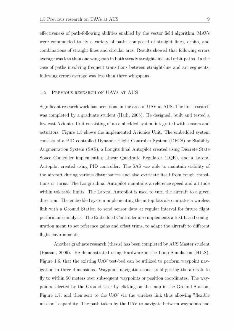
Another graduate research (thesis) has been completed by AUS Master student
(Hassan, 2006). He demonstrated using Hardware in the Loop Simulation (HILS),
Figure 1.6, that the existing UAV test-bed can be utilized to perform waypoint nav-
igation in three dimensions. Waypoint navigation consists of getting the aircraft to
fly to within 50 meters over subsequent waypoints or position coordinates. The way-
points selected by the Ground User by clicking on the map in the Ground Station,
Figure 1.7, and then sent to the UAV via the wireless link thus allowing ”flexible
mission” capability. The path taken by the UAV to navigate between waypoints had

1.5 Previous research on UAVs at AUS 10
Figure 1.5: AUS Avionics Unit constructed in (Hadi, 2005)
to be smooth and fast and doesn’t violate the flight constraints of the UAV.
Figure 1.6: The HILS Setup designed in (Hassan, 2006)
1.6 Thesis objectives and contribution 11
Figure 1.7: The Ground Station Built in (Hassan, 2006)
1.6 Thesis objectives and contribution
As shown in Figure 1.8, the UAV system architecture considered in this thesis consists
of five layers: the Waypoint Path Planner (WPP), the Dynamic Trajectory Smoother
(DTS), the Trajectory Tracker (TT), the Longitudinal and Lateral Autopilots, and
the UAV. The description and the role of each is listed below:
Waypoint Path Planner (WPP) The WPP generates waypoint paths (straight-
line segments) that change in accordance with the dynamic environment con-
sisting of the location of the UAV, the targets, and the dynamically changing
threats.
Dynamic Trajectory Smoother (DTS) The DTS smoothes through these way-
points and produces a feasible time parameterized desired trajectory, that is,
the desired position, heading, and altitude.
Trajectory Tracker (TT) The TT outputs the desired velocity command, head-
ing command, and altitude command to the autopilots based on the desired

1.7 Thesis outline 12
trajectory.
Longitudinal and Lateral Autopilots The autopilots then use these commands
to control the elevator, aileron, rudder deflections and the throttle setting of
the UAV.
UAV The UAV model which will be identified to get the mathematical model. This
mathematical model will be used to develop and integrate the above layers
together in the designed HILS.
Figure 1.8: UAV System Architecture
Where the objectives of this thesis is building a model of the ARF60 UAV,
designing the longitudinal and lateral autopilots and implementing the trajectory
tracker. The integration of the above layers was validated using the hardware in the
loop simulation which was developed as well.
1.7 Thesis outline
This thesis is organized as follows. Chapter 2 explains the nonlinear mathematical
model and dynamics equations. The ARF60 AUS-UAV modeling and system iden-
tifications is addressed in Chapter 3. The controller design, and simulation of the
ARF60 AUS-UAV are in Chapter 4. Chapters 5-6 cover the move from simulation to

1.7 Thesis outline 13
a hardware platform through the hardware in the loop simulation (HILS). Hardware
results of real-time trajectory tracking are presented in Chapter 7. Conclusions and
recommendations for future work are addressed in Chapter 8.

Chapter 2
ARF60 AUS-UAV Nonlinear Model and
Dynamics Equations
2.1 UAV Coordinate Frames and Axis System Definition
Before developing the nonlinear dynamic model of the aircraft, several coordinate
frames and axes must be defined.
In this section, the inertial frame, the body frame, the stability frame and the wind
frame will be described first.
2.1.1 Inertial Frame
With reference to Figure 2.1, the inertial axis system, Fi(OiXiYiZi) is an earth fixed
coordinate system. Its origin Oi is located at some point on the earth surface. With
the positive Zi directed toward the center of the earth. the positive Xi directed
to the north and perpendicular to Zi while the positive Yi directed to the east and
perpendicular to the XiZi (Peddle, 2005). In this thesis, the earth is assumed to be
flat and not rotating since our UAV flight ranges aren’t significantly large (1-3Km).
2.1.2 Body Frame
FB(OBXBYBZB) is the body frame with its origin is the CG (Center of Gravity) of
the UAV. The positive XB axis directing out of the nose of the UAV, the positive YB
perpendicular to XB and directing out of the right wing while the positive ZB axis is
out of the UAV frame pointing downward and perpendicular to the XBYB plane.
The UAV is said to Roll about the XB-axis, Pitch about the YB, Yaw about
the ZB. The axes definition of the stability frame is shown in Figure 2.2.

2.1 UAV Coordinate Frames and Axis System Definition 15
Figure 2.1: Inertial Axis Definition
Figure 2.2: Body Axis Definition
2.1.3 Stability Frame
When the XB axis of the body frame pitch with α angle of attack (AOA) then the
body axis frame is referred to as Stability Frame FS(OSXSYSZS) as shown in Figure
2.3.
Stability frame generates the aerodynamic forces, and thus reducing the aerodynamic
model to its simplest form.

2.1 UAV Coordinate Frames and Axis System Definition 16
Figure 2.3: Stability Axis Definition
Figure 2.4: Wind Axis Definition
2.1.4 Wind Frame
Whenever the Body Frame faces a wind, it is going to yaw into the wind with β Angle
of Sideslip. Then the body axis frame is referred to as Wind Frame FW (OWXWYWZW ).
The wind frame axes definition is illustrated in Figure 2.4.
The following relations are useful and good to be introduced at this point:
Vair =√U2 + V 2 +W 2 (2.1)

2.2 UAV Aerodynamic Control Surfaces 17
Figure 2.5: Control Surface Deflection
α = arctan(W
U) (2.2)
β = arcsin(V
Vair
) (2.3)
2.2 UAV Aerodynamic Control Surfaces
The conventional aerodynamic control surface deflection variables will be defined also
with reference to Figure 2.5.
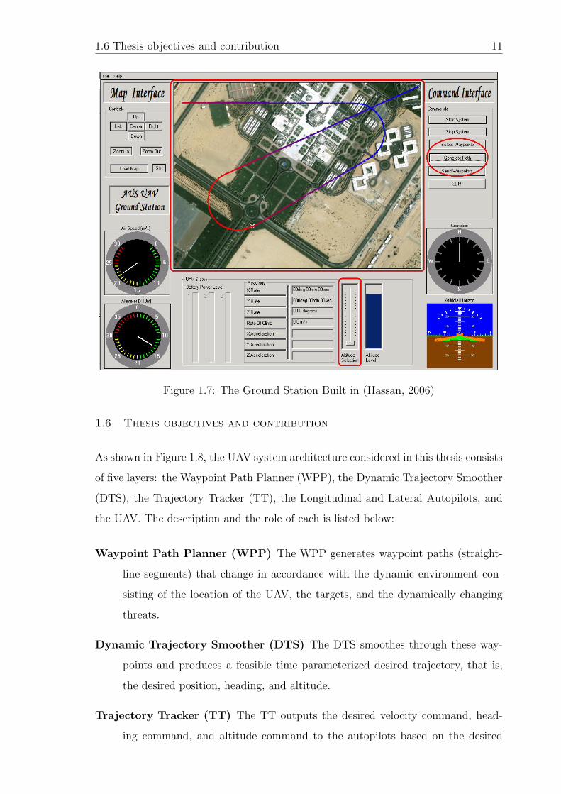
• δa-Aileron Control Surface Deflection Angle.
Positive deflection causes a negative rolling moment. Ailerons can be used to
generate a rolling motion for the UAV.
Ailerons are used to bank the UAV; to cause one wing tip to move up and the
other wing tip to move down. The banking creates an unbalanced side force
component of the large wing lift force which causes the UAV’s flight path to
curve.
With greater downward deflection, the lift will increase in the upward direction.
Figure 2.6 shows the aileron on the left wing deflected down while the aileron
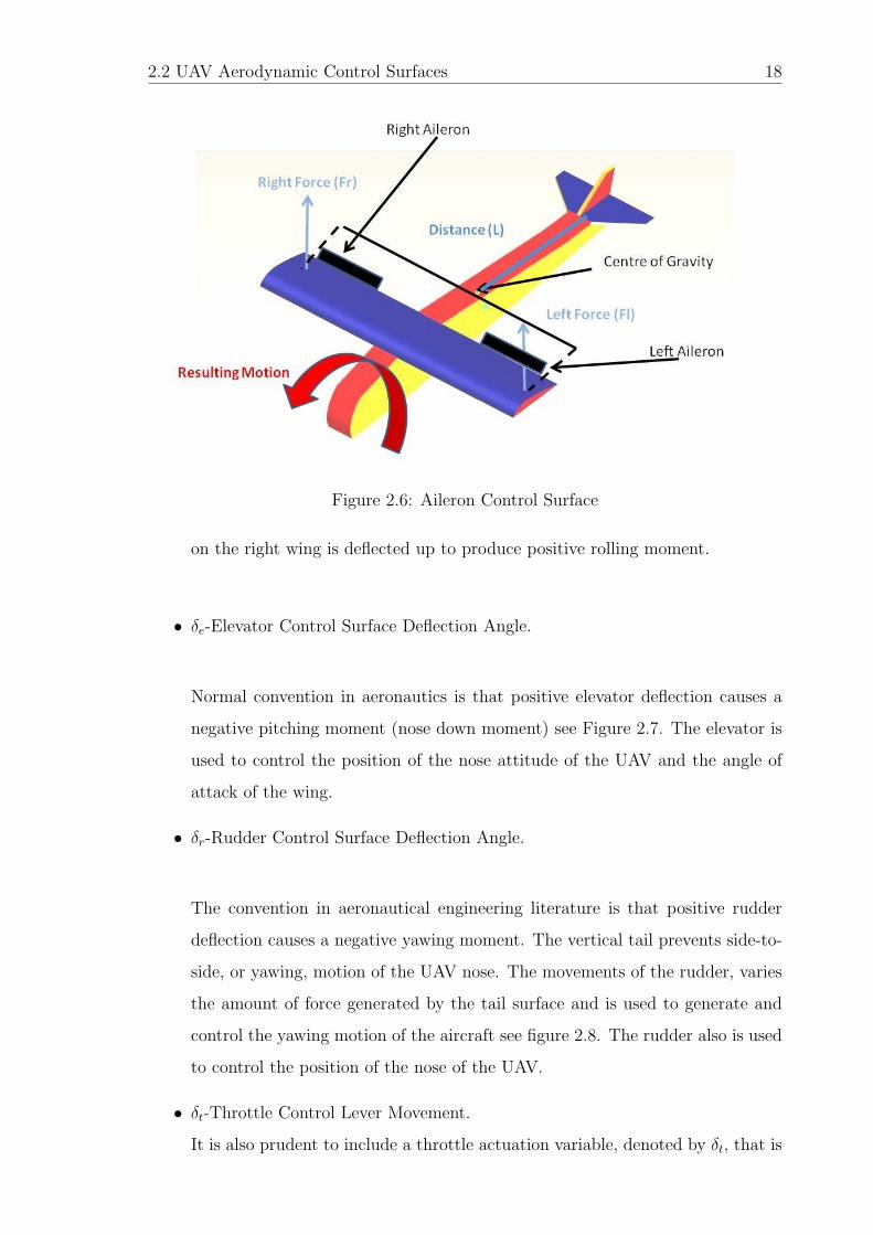
2.2 UAV Aerodynamic Control Surfaces 18
Figure 2.6: Aileron Control Surface
on the right wing is deflected up to produce positive rolling moment.
• δe-Elevator Control Surface Deflection Angle.
Normal convention in aeronautics is that positive elevator deflection causes a
negative pitching moment (nose down moment) see Figure 2.7. The elevator is
used to control the position of the nose attitude of the UAV and the angle of
attack of the wing.
• δr-Rudder Control Surface Deflection Angle.
The convention in aeronautical engineering literature is that positive rudder
deflection causes a negative yawing moment. The vertical tail prevents side-to-
side, or yawing, motion of the UAV nose. The movements of the rudder, varies
the amount of force generated by the tail surface and is used to generate and
control the yawing motion of the aircraft see figure 2.8. The rudder also is used
to control the position of the nose of the UAV.
• δt-Throttle Control Lever Movement.
It is also prudent to include a throttle actuation variable, denoted by δt, that is

2.2 UAV Aerodynamic Control Surfaces 19
Figure 2.7: Elevator Control Surface
Figure 2.8: Rudder Control Surface

2.3 UAV Equations of Motion 20
related to the output of the magnitude of the UAV thrust vector.
The movement of the throttle lever range is between (0-1), where the two limits
correspond to engine cutoff and full throttle respectively.
2.3 UAV Equations of Motion
The basis for analysis, computation, and simulation of the motions of the UAV as
well as autopilot design is the mathematical model of the UAV and its subsystems.
Actual UAV systems are highly complicated nonlinear systems. It consists of an
aggregate of elastic bodies so connected that both rigid and elastic relative motions
can occur. For example, the propeller rotates, control surfaces move about their
hinges, and bending and twisting of the various aerodynamic surfaces occur. The
external forces that act on the UAV are also complex functions of shape and motion.
Realistic analysis of engineering precision are not likely to be accomplished with a
very simple mathematical model. The model that is developed in the following section
is a classical model. It has been found by aeronautical engineers and researchers to
be very useful in practise. The vehicle is treated as a single rigid body with six degree
of freedom. This body is free to move in the atmosphere under the actions of gravity
and aerodynamic forces.
As indicated earlier in section 2.1, the Earth is treated as flat and stationary in inertial
space. These assumptions simplify the model enormously, and are quite acceptable
for analyzing most problems of UAV flight (Peddle, 2005).
2.3.1 UAV Forces and Moments
Newton’s second law of motion is used to determine the effect of the net force and
moment on a body. It states that the summation of all external forces acting on a
body is equal to the time rate of change of the linear momentum of the body, and
the summation of the external moments acting on the body is equal to the time rate
of change of the angular momentum.
The summary of the equations consists of three forces and moments equations
are expressed in matrix form in Equations 2.4 and 2.5 respectively.
2.3 UAV Equations of Motion 21
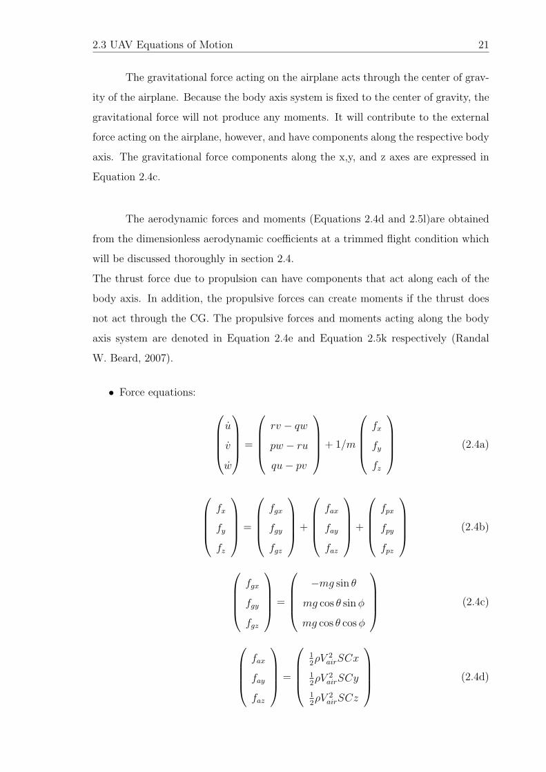
The gravitational force acting on the airplane acts through the center of grav-
ity of the airplane. Because the body axis system is fixed to the center of gravity, the
gravitational force will not produce any moments. It will contribute to the external
force acting on the airplane, however, and have components along the respective body
axis. The gravitational force components along the x,y, and z axes are expressed in
Equation 2.4c.
The aerodynamic forces and moments (Equations 2.4d and 2.5l)are obtained
from the dimensionless aerodynamic coefficients at a trimmed flight condition which
will be discussed thoroughly in section 2.4.
The thrust force due to propulsion can have components that act along each of the
body axis. In addition, the propulsive forces can create moments if the thrust does
not act through the CG. The propulsive forces and moments acting along the body
axis system are denoted in Equation 2.4e and Equation 2.5k respectively (Randal
W. Beard, 2007).
• Force equations: u
v
w
=
rv − qw
pw − ru
qu− pv
+ 1/m
fx
fy
fz
(2.4a)
fx
fy
fz
=
fgx
fgy
fgz
+
fax
fay
faz
+
fpx
fpy
fpz
(2.4b)
fgx
fgy
fgz
=
−mg sin θ
mg cos θ sinφ
mg cos θ cosφ
(2.4c)
fax
fay
faz
=
12ρV 2
airSCx
12ρV 2
airSCy
12ρV 2
airSCz
(2.4d)
2.3 UAV Equations of Motion 22
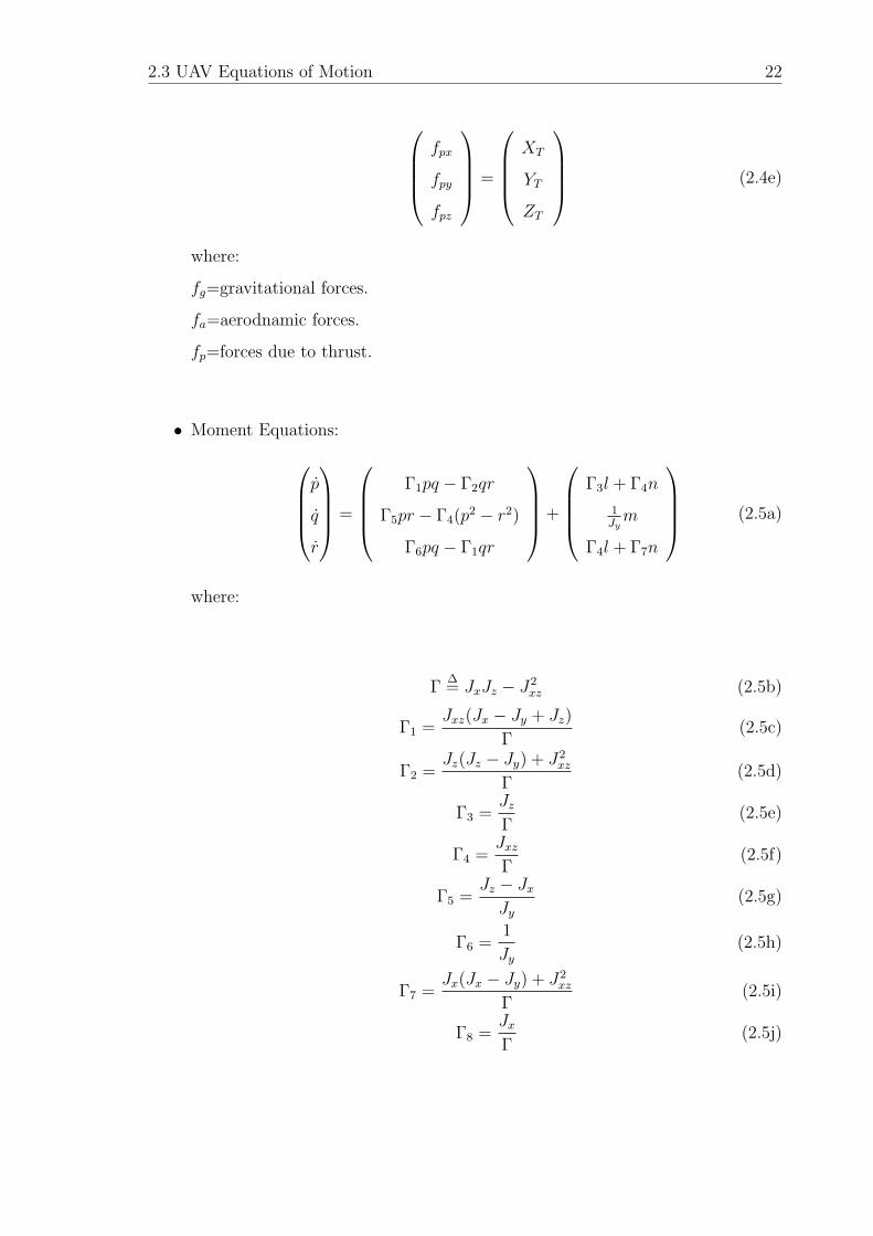
fpx
fpy
fpz
=
XT
YT
ZT
(2.4e)
where:
fg=gravitational forces.
fa=aerodnamic forces.
fp=forces due to thrust.
• Moment Equations:p
q
r
=
Γ1pq − Γ2qr
Γ5pr − Γ4(p2 − r2)
Γ6pq − Γ1qr
+
Γ3l + Γ4n
1Jym
Γ4l + Γ7n
(2.5a)
where:
Γ∆= JxJz − J2
xz (2.5b)
Γ1 =Jxz(Jx − Jy + Jz)
Γ(2.5c)
Γ2 =Jz(Jz − Jy) + J2
xz
Γ(2.5d)
Γ3 =Jz
Γ(2.5e)
Γ4 =Jxz
Γ(2.5f)
Γ5 =Jz − Jx
Jy
(2.5g)
Γ6 =1
Jy
(2.5h)
Γ7 =Jx(Jx − Jy) + J2
xz
Γ(2.5i)
Γ8 =Jx
Γ(2.5j)

2.3 UAV Equations of Motion 23
Lp
Mp
Np
=
LT
MT
NT
(2.5k)
l
m
n
=
12ρV 2
airSbCl
12ρV 2
airScCm
12ρV 2
airSbCn
(2.5l)
2.3.2 UAV Orientation and Position
• Kinematic Equations: The orientation of the airplane can be described by three
consecutive rotations whose order is important. The angular rotations are called
the Euler angles.
The relationship between the angular velocities in the body frame (p, q and r)
and the Euler rates (ψ, θ, and φ) is shown in Equation 2.6.
p
q
r
=
1 0 − sin θ
0 cosφ cos θ sinφ
0 − sinφ cos θ cosφ
φ
θ
ψ
(2.6)
Equation 2.6 can be solved for the Euler rates in terms of the body angular
velocities:
φ
θ
ψ
=
1 sinφ tan θ cosφ tan θ
0 cosφ − sinφ
0 sinφ sec θ cosφ sec θ
p
q
r
(2.7)
By integrating theses equations, one can determine the Euler angles ψ, θ, and
φ.
• Navigation Equations: The state variables pn, pe, and pd are inertial frame
position quantities, whereas the velocities u, v, and w are body frame quantities.
Therefore the relationship between the postilion and velocities if we account
for the wind (wn, we, and wd) represented in the inertial frame is given by
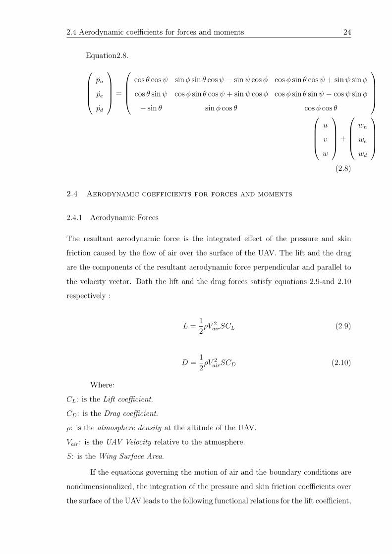
2.4 Aerodynamic coefficients for forces and moments 24
Equation2.8.pn
pe
pd
=
cos θ cosψ sinφ sin θ cosψ − sinψ cosφ cosφ sin θ cosψ + sinψ sinφ
cos θ sinψ cosφ sin θ cosψ + sinψ cosφ cosφ sin θ sinψ − cosψ sinφ
− sin θ sinφ cos θ cosφ cos θ
u
v
w
+
wn
we
wd
(2.8)
2.4 Aerodynamic coefficients for forces and moments
2.4.1 Aerodynamic Forces
The resultant aerodynamic force is the integrated effect of the pressure and skin
friction caused by the flow of air over the surface of the UAV. The lift and the drag
are the components of the resultant aerodynamic force perpendicular and parallel to
the velocity vector. Both the lift and the drag forces satisfy equations 2.9-and 2.10
respectively :
L =1
2ρV 2
airSCL (2.9)
D =1
2ρV 2
airSCD (2.10)
Where:
CL: is the Lift coefficient.
CD: is the Drag coefficient.
ρ: is the atmosphere density at the altitude of the UAV.
Vair: is the UAV Velocity relative to the atmosphere.
S: is the Wing Surface Area.
If the equations governing the motion of air and the boundary conditions are
nondimensionalized, the integration of the pressure and skin friction coefficients over
the surface of the UAV leads to the following functional relations for the lift coefficient,

2.5 Implementation of the ARF60 AUS-UAV Nonlinear Model in Simulink 25
the drag coefficient and the side force coefficient for a constant geometry UAV:
CL = CL + CLαα+ CLδeδe +
c
2Vair
(CLαα+ CLqq) (2.11)
CD = CD +(CL − CL)
2
πeAR+ CDδa
δa + CDδeδe + CDδr
δr (2.12)
CY = CYββ + CYδa
δa + CYδrδr +
b
2Vair
(CYpp+ CYrr) (2.13)
2.4.2 Aerodynamic Moments
The aerodynamic moments are build from the following moment coefficients:
Cl = Clββ + Clδaδa + Clδr
δr +b
2Vair
(Clpp+ Clrr) (2.14)
Cm = Cm + Cmαα+ Cmδeδe +
c
2Vair
(Cmαα+ Cmqq) (2.15)
Cn = Cnββ + Cnδa
δa + Cnδrδr +
b
2Vair
(Cnpp+ Cnrr) (2.16)
2.5 Implementation of the ARF60 AUS-UAV Nonlinear Model in Simulink
The forces and moments described in Section 2.3 can now be implemented in Simulink
environment. Simulink block-diagrams, are flexible, and more user-friendly than other
models proposed in the literature (Rauw, 1992). With the presence of the Aerosim and
Aerospace Simulink based Blocksets, adding new output equations, deleting unwanted
relations, or changing sub models to implement other aircraft is now straightforward.
Figure 2.9, shows the general structure of the ARF60 AUS-UAV Simulink nonlinear
model.
Most of the subsystems were designed using the AeroSim and Aerospace
blocks. The propulsion and actuators models were modelled experimentally as it will
be described in the System identification chapter 3. The aerodynamics, propulsion,
and inertia models compute the airframe loads (forces and moments) as functions of

2.5 Implementation of the ARF60 AUS-UAV Nonlinear Model in Simulink 26
Figure 2.9: ARF60 UAV Simulink Model general Structure
control inputs and environment (atmosphere and Earth) effects. The resulting accel-
erations are then integrated by the Equations of Motion to obtain the aircraft states
(position, velocity, attitude, angular velocities). The aircraft states will affect the
output of the environment blocks at the next iteration (for example altitude changes
result in atmospheric pressure changes, latitude and longitude variations result in
gravity variations). Also, the aircraft states are used in the computation of sensor
outputs (GPS, inertial measurements, etc.).
Chapter 3
ARF60 AUS-UAV Modeling and System
Identifications
After introducing the dynamics of a conventional aircraft in Chapter 2, this chapter
provides the identified model that reflects our ARF60 AUS-UAV. This identification
includes, aerodynamic parameters, mass moment of inertia, propulsion model and the
actuators models.
3.1 Introduction
One of the oldest and most fundamental of all human scientific pursuits is devel-
oping mathematical models for physical systems based on imperfect observations or
measurements. This activity is known as system identification. A good practical
definition is that of (Zadeh, 2007):
System identification is the determination, on the basis of observation of
input and output, of a system within a specified class of systems to which
the system under test is equivalent.
Implicit in the preceding definition is the practical fact that the mathematical model
of a physical system is not unique. In general, the guiding principle for model se-
lection is the parsimony principle, which states that of all models is specified class
that exhibit the desired characteristics, the simplest one should be preferred. There
are both theoretical and practical reasons for the parsimony principle, and these were
discussed further throughout (Vladislav Klein & Eugene A. Morell, 2006). The pre-
ceding definition also mentions that system identification is based on observations
of input and output for the system under test. In practise, these observations are
corrupted by measurement noise.

3.2 Overview of UAV System ID and literature Review 28
The most important requirement for a mathematical model is that it be useful
in some way. This means that the model can be used to predict some aspects of the
behavior of a physical system, while at other times it can just predict the values of
desired parameters. In any case, the synthesized model must be simple enough to be
useful and at the same time complex enough to capture important dependencies and
features embodied in the observations or measurements.
3.2 Overview of UAV System ID and literature Review
In aircraft dynamics and control, system identification techniques are used to obtain
refined aerodynamic model, propulsion system model, and control actuators models
as shown in Figure 3.1.
In the present investigation, the identification model will be used in the fol-
lowing objectives:
1. Find the system mathematical model S, given the input u and the output y.
2. Find the input u to get the output y, given the system mathematical model S
(for the autopilot system design)
3. Find the output y for the input u, given the system mathematical model S(for
the hardware in the loop simulation).
As indicated earlier in Chapter 2 an aircraft can be modeled as a rigid body,
whose motion is governed by Newton laws. System identification techniques need
to be used to characterize applied forces and moments acting on the aircraft that
arise from aerodynamics and propulsion. Typically, thrust forces and moments are
obtained from ground tests, so aircraft system identification is applied to model the
functional dependence of aerodynamic forces and moments on aircraft motion and
control variables. Modern computational methods and wind-tunnel can provide, in
many instances, comprehensive data about the aerodynamic characteristics of an
aircraft. However, there are still several motivations for identifying aircraft models
from flight-test data, including

3.2 Overview of UAV System ID and literature Review 29
Figure 3.1: UAV components dynamics and control
1. Verifying and interpreting theoretical predictions and wind-tunnel test results
(flight-test results can also be used to help improve ground based predictive
methods);
2. Obtaining more accurate and comprehensive mathematical models of aircraft
dynamics, for use in designing stability augmentation system and flight control
systems;
3. Developing flight simulators, which require accurate representation of the air-
craft in all flight modes and regimes (many aircraft motions and flight conditions
simply cannot be duplicated in the wind tunnel nor computed analytically with
sufficient accuracy or computational efficiency);
4. Verifying aircraft specification compliance.
Recently, several papers discussed new system identification algorithms. Those
techniques have been proposed for the modelling of nonlinear systems. Fuzzy identifi-
cation (Li-Xin Wang, 1995), state space identification (Shaaban, A., 2006), frequency
domain analysis (R. Pintelon & J. Schoukens., 2001), artificial neural networks are
3.3 System ID steps 30
some of the prominent ones. On the other hand, in (Chunhua Hu & Zhu, 2004) they
used an easy to implement system identification process. System identification for a
small UAVs take-off process based on operator’s control was carried out. The auto-
regressive exogenous ARX, auto-regressive moving average exogenous ARMAX and
Box-Jenkins BJ models were used to describe the dynamics of BlueEagles speeding
up before take-off where they have better input-output fits. Using input and output
data of actual flying test, system identification results were shown through numerical
analysis. Validated by input and output data of other actual flying test, the resulting
model was acceptable.
3.3 System ID steps
The System Identification problem is to estimate a model of a system based on ob-
served input-output data. Several ways to describe a system and to estimate such de-
scriptions exist. This section gives a brief account of the most important approaches.
The procedure to determine a model of a dynamical system from observed input-
output data involves three basic ingredients. Which are input-output measurement
data, set of candidate structure models and identification method selection.
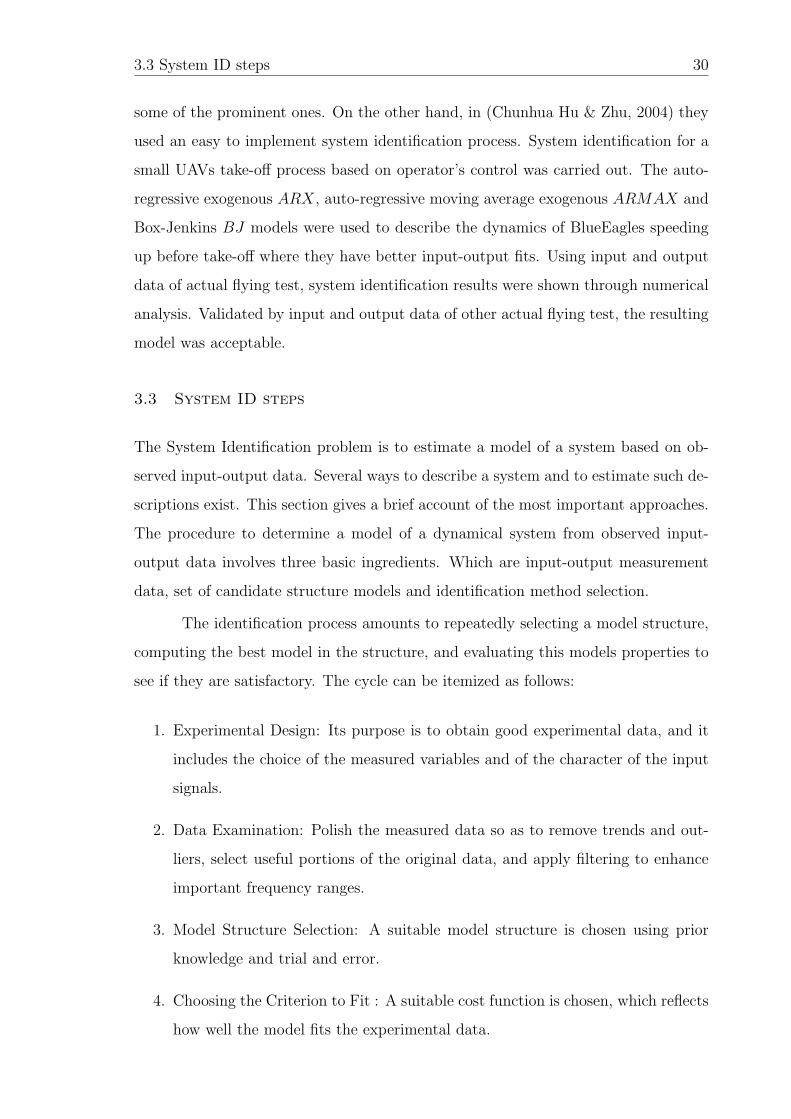
The identification process amounts to repeatedly selecting a model structure,
computing the best model in the structure, and evaluating this models properties to
see if they are satisfactory. The cycle can be itemized as follows:
1. Experimental Design: Its purpose is to obtain good experimental data, and it
includes the choice of the measured variables and of the character of the input
signals.
2. Data Examination: Polish the measured data so as to remove trends and out-
liers, select useful portions of the original data, and apply filtering to enhance
important frequency ranges.
3. Model Structure Selection: A suitable model structure is chosen using prior
knowledge and trial and error.
4. Choosing the Criterion to Fit : A suitable cost function is chosen, which reflects
how well the model fits the experimental data.
3.4 Aircraft System ID 31
5. Parameter estimation: An optimization problem is solved to obtain the numer-
ical values of the model parameters.
6. Model validation: The model is tested in order to reveal its validity.
Figure 3.2: System Identification Steps
A flow chart describing the previous steps is shown in Figure 3.2. If the model
is good enough, then the work is completed; otherwise we go back to Step 3 and
try another model. Possibly, we can try other estimation methods (Step 4) or work
further on the input-output data (Steps 1 and 2).
3.4 Aircraft System ID
3.4.1 Aerodynamic Numerical modeling
Aircraft aerodynamics can be modeled using linear coefficients estimated based on
aircraft geometry. Aircraft mass and CG location are too important quantities that
need to be identified. The center of gravity location was carefully determined in the
body axes,it was taken at the point where the aircraft has a static balance. As shown
in Figures 3.3 two lines were drawn on the two planes (x-y & x-z). Another line
was drawn on the (x-y) to get the intersection with the depth of the (x-z) mark;
Figure 3.4. The gross and empty weight of the UAV and the landing wheels were

3.4 Aircraft System ID 32
Figure 3.3: CG location Experiment top
measured using a precise scale. The added masses ie.IMU,Autopilot,batteries, etc.
were weighed later. All of this data listed in Table 3.1 was entered to MATLAB
script to estimate the stability derivatives. The stability derivatives resulted from
the MATLAB script based on the linearized model of the aerodynamic forces and
moments are summarized in Table 3.2
Figure 3.4: CG location Experiment
3.4 Aircraft System ID 33
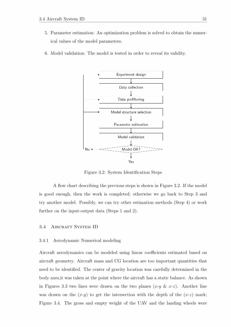
Table 3.1: ARF60 measured geometric parameters - input to the MATLAB script
Property Symbol Value Unit(SI)
Empty Aircraft Mass (without fuel) mE 3.416 KgGross Aircraft Mass (with fuel) mG 3.5105 Kg
Center of Gravity Location (x, y, z) CG [0.00 0.00 0.00] mRoll Inertia Ixx 0.19969 kg.m2
Pitch Inertia Iyy 0.24086 kg.m2
Yaw Inertia Izz 0.396 kg.m2
Wing
Length of Mean Aerodynamic Cord C 0.324 mWing Span b 1.87 m
Wing Dihedral Angle Γ 6 degWing Taper Ratio λ 1 −Wing Surface Area S 0.6059 m2
Ailerons Surface Area Sa 0.0581 m2
Ailerons Around Area Aa 0.4277 m2
Horizontal TailHorizontal Tail Span bt 0.6700 m
Horizontal Tail Mean Aerodynamic Cord Ct 0.1950 mHorizontal Tail Area St 0.1307 m2
Elevator Surface Area Se 0.0232 m2
Distance from CG to H.Tail Quarter Cord lt 0.8200 mHorizontal Tail Volume Ratio VH 0.5457 −
Vertical TailVertical Tail Span bv 0.2350 m
Vertical Tail Mean Aerodynamic Cord Cv 0.2150 mVertical Tail Area Sv 0.0505 m2
Rudder Surface Area Sr 0.1307 m2
Distance from CG to V.Tail Aerodynamic Center lt 0.8400 mVertical Tail Volume Ratio Vv 0.2162 −
3.4.2 Flight Tests Based System ID
Experimental Design
Several flight tests for system identification were conducted. The block diagram for
system identification is shown in Figure 3.5, where δa, δe, δr, δt are input signals for
identification and the euler angles: φ, θ, ψ, accelerations: ax, ay, az, angular rates:
p, q, r, position: Lat, Lon, Alt, speed: Vx, Vy, Vz, Static and differential pressure for
altitude and true airspeed are the output signals for identification. Extensive flying
tests were conducted, from which, one data set was selected for system identification.
The input data acquired from this experiment is shown in Figure 3.6. This data shows
the actual deflections of the actuators according to the servo inputs commanded by

3.4 Aircraft System ID 34
Table 3.2: Stability derivatives of the ARF60 UAV (All units per radian)
Symbol Derivative Value
Lift coefficientCL Zero alpha lift 0.4100CLα Alpha derivative 4.3842CLαt
Alpha derivative for the tail 3.6369CLαv
Alpha derivative for the vertical tail 0.9114CLδe
Pitch control (elevator) derivative 0.3059CLα
Alpha-dot derivative 0CLq Pitch rate derivative 0.6431
Drag coefficientCD Minimum drag 0.0500CDδe
Pitch control (elevator) derivative 0CDδa
Roll control (aileron) derivative 0CDδr
Yaw control (rudder) derivative 0Side force coefficient
CYβSideslip derivative -0.1795
CYδaRoll control derivative 0
CYδrYaw control derivative 0.1132
CYp Roll rate derivative 0CYrr Yaw rate derivative 0
Pitch moment coefficientCm Zero alpha pitch 0Cmα Alpha derivative 0Cmδe
Pitch control derivative -0.7741Cmα
Alpha dot derivative -6.0730Cmq Pitch rate derivative -10.0467
Roll moment coefficientClβ Sideslip derivative -0.0013Clδa
Roll control derivative 0.8275Clδr
Yaw control derivative 0.0036Clp Roll rate derivative -1.8267Clr Yaw rate derivative 0.0052
Yaw moment coefficientCnβ
Sideslip derivative 0.4653Cnδa
Roll control derivative -0.1357Cnδr
Yaw control derivative -0.2934Cnp Roll rate derivative -1.8267Cnr Yaw rate derivative -0.2934
the pilot. we tried to excite the aircraft dynamics by introducing series of doublets
on the aileron, elevator, rudder and throttle actuators. The output data according to
this input signals are shown in Figures 3.7-3.12.
The aerodynamic coefficients are identified from real flight tests using mea-
surements from accelerometers and rate gyros. The aerodynamic force coefficients are

3.4 Aircraft System ID 35
Figure 3.5: Construction of System identification for the ARF60 UAV
Figure 3.6: ARF60 Actuators deflections during the system identification test
calculated in the body frame using Equations 3.1 by assuming that the thrust force

3.4 Aircraft System ID 36
Figure 3.7: ARF60 Angular Rates during the system identification test
Figure 3.8: ARF60 Accelerations during the system identification test

3.4 Aircraft System ID 37
Figure 3.9: ARF60 Attitudes during the system identification test
Figure 3.10: ARF60 Velocities during the system identification test

3.4 Aircraft System ID 38
Figure 3.11: ARF60 Position during the system identification test
Figure 3.12: ARF60 Air Data during the system identification test

3.4 Aircraft System ID 39
is applied only along the body x-axis.
CX =m
qSax −
T
qS(3.1a)
CY =m
qSay (3.1b)
CZ =m
qSaz (3.1c)
The aerodynamic moment coefficients are also calculated in the body frame
using Equations 3.2 where L,MandN are calculated using Equation 2.5.
C` =L
qSb(3.2a)
Cm =M
qSc(3.2b)
Cn =N
qSb(3.2c)
After identifying the aerodynamic Force/Moment coefficients, a linear regres-
sion model was derived based on the decoupled longitudinal and lateral dynamics of
the aircraft (Dongwon Jung & Panagiotis Tsiotras, 2007). The formed regressions
model is expressed in Equations 3.3
CX = Cx + Cxαα+ Cxq
c
2VT
q + Cxδeδe (3.3a)
CY = Cy + Cyββ + Cyp
b
2VT
p+ Cyr
b
2VT
r + Cyδaδa+ Cyδr
δr (3.3b)
CZ = Cz + Czαα+ Czq
c
2VT
q + Czδeδe (3.3c)
C` = CL + C`ββ + C`p
b
2VT
p+ C`r
b
2VT
r + C`δaδa+ C`δr
δr (3.3d)
Cm = Cm + Cmαα+ Cmq
c
2VT
q + Cmδeδe (3.3e)
Cn = Cn + Cnββ + Cnp
b
2VT
p+ Cnr
b
2VT
r + Cnδaδa+ Cnδr
δr (3.3f)
From Equations 3.3, it is clear that each aerodynamic coefficient is a func-
tion of decoupled longitudinal and lateral derivatives, where the stability and control
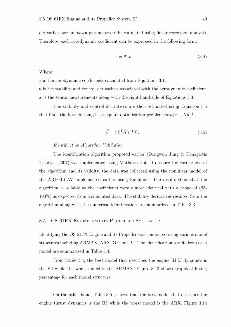
3.5 OS 61FX Engine and its Propeller System ID 40
derivatives are unknown parameters to be estimated using linear regression analysis.
Therefore, each aerodynamic coefficient can be expressed in the following form:
z = θTx (3.4)
Where:
z is the aerodynamic coefficients calculated from Equations 3.1.
θ is the stability and control derivatives associated with the aerodynamic coefficient
x is the sensor measurements along with the right-hand-side of Equations 3.3.
The stability and control derivatives are then estimated using Equation 3.5
that finds the best fit using least-square optimization problem min‖z −Xθ‖2.
θ = (XTX)−1Xz (3.5)
Identification Algorithm Validation
The identification algorithm proposed earlier (Dongwon Jung & Panagiotis
Tsiotras, 2007) was implemented using Matlab script. To assure the correctness of
the algorithm and its validity, the data was collected using the nonlinear model of
the ARF60-UAV implemented earlier using Simulink. The results show that the
algorithm is reliable as the coefficients were almost identical with a range of (95-
100%) as expected from a simulated data. The stability derivatives resulted from the
algorithm along with the numerical identification are summarized in Table 3.3.
3.5 OS 61FX Engine and its Propeller System ID
Identifying the OS 61FX Engine and its Propeller was conducted using various model
structures including ARMAX, ARX, OE and BJ. The identification results from each
model are summarized in Table 3.4.
From Table 3.4, the best model that describes the engine RPM dynamics is
the BJ while the worst model is the ARMAX. Figure 3.13 shows graphical fitting
percentage for each model structure.
On the other hand, Table 3.5 , shows that the best model that describes the
engine thrust dynamics is the BJ while the worst model is the ARX. Figure 3.14

3.5 OS 61FX Engine and its Propeller System ID 41
Table 3.3: Identified Stability derivatives of the ARF60 UAV (All units per radian)using System ID algorithm
Symbol ID Algorithm Value Numerical ID Value
Lift coefficientCL 0.41 0.4100CLα 4.38416 4.3842CLδe
0.30585 0.3059CLq 1.096 0.6431
Drag coefficientCD 0.0510 0.0500CDδe
-0.0106 0CDδa
2.55e-04 0CDδr
2.188e-04 0Side force coefficient
CYβ-0.17947 -0.1795
CYδa-2.30e-14 0
CYδr0.1131 0.1132
CYp 1.87e-12 0CYrr 3.02e-15 0
Pitch moment coefficientCm 0.0022 0Cmα -1.09172 0Cmδe
-0.7064 -0.7741Cmq -16.5758 -10.0467
Roll moment coefficientClβ 0.00126 -0.0013Clδa
2.06861e-05 0.8275Clδr
0.00363 0.0036Clp -0.7306 -1.8267Clr 0.00517 0.0052
Yaw moment coefficientCnβ
0.46531 0.4653Cnδa
-3.392e-06 -0.1357Cnδr
-0.2934 -0.2934Cnp 0.5480 -1.8267Cnr -0.3712 -0.2934
Table 3.4: OS 61FX Engine RPM System ID Results
Model Model Structure Fitting %
ARX arx525 85.38%ARMAX amx5111 84.4 %
OE oe2210 84.91%BJ bj11232 85.31%
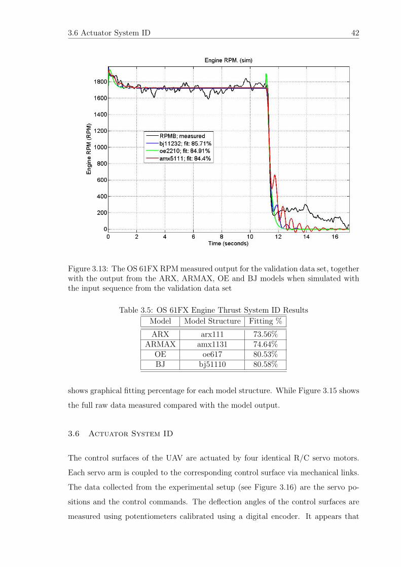
3.6 Actuator System ID 42
Figure 3.13: The OS 61FX RPM measured output for the validation data set, togetherwith the output from the ARX, ARMAX, OE and BJ models when simulated withthe input sequence from the validation data set
Table 3.5: OS 61FX Engine Thrust System ID Results
Model Model Structure Fitting %
ARX arx111 73.56%ARMAX amx1131 74.64%
OE oe617 80.53%BJ bj51110 80.58%
shows graphical fitting percentage for each model structure. While Figure 3.15 shows
the full raw data measured compared with the model output.
3.6 Actuator System ID
The control surfaces of the UAV are actuated by four identical R/C servo motors.
Each servo arm is coupled to the corresponding control surface via mechanical links.
The data collected from the experimental setup (see Figure 3.16) are the servo po-
sitions and the control commands. The deflection angles of the control surfaces are
measured using potentiometers calibrated using a digital encoder. It appears that

3.6 Actuator System ID 43
Figure 3.14: The OS 61FX thrust measured output for the validation data set, to-gether with the output from the ARX, ARMAX, OE and BJ models when simulatedwith the input sequence from the validation data set
Figure 3.15: Thrust measured output together with the output from the BJ modelwhen simulated with the input PRBS

3.6 Actuator System ID 44
Figure 3.16: Actuator Identifcation Setup
an R/C servo motor nearly performs a dead beat control action. Thus, a first-order
low pass filter and control saturation results in a good actuator model. Results of all
control surfaces models are summarized in Appendix C.1.1.

Chapter 4
ARF60 AUS-UAV Aircraft Natural Motion,
Controller Design and Simulation
In this chapter we study the stick fixed motion, that is, the motion of the aircraft
when all control surfaces are locked in position. Moreover, the aircraft response
to actuation of primary controls elevator, aileron, rudder, and throttle also will be
studied. The analysis of both the longitudinal and lateral models will be presented in
detail in Section 4.1. Next, the autopilot design is considered with linear simulation
results in Section 4.2.
4.1 Aircraft Linear Model
The state space linear model of the aircraft was derived using the already available
stability derivatives found in Section 3.4.1. The linearized state space model is needed
to develop the guidance and control laws. It is used to develop airspeed hold, altitude
hold as well as for ground and navigation control. The nonlinear aircraft model is
linearized about the trim condition. The derived linear model is then decoupled into
a longitudinal and lateral models. The following longitudinal and lateral models were
linearized around a typical flight condition (Va = 20m/s, h = 100m, and φ = 0).
4.1.1 ARF60 UAV Longitudinal Model
The following state space model is the linear longitudinal model for the ARF60 UAV:

4.1 Aircraft Linear Model 46
u
w
q
θ
h
=
−0.2289 0.3712 0 −9.81 0
−1.8772 −10.1512 20 0 0
0.9219 −7.0403 −26.072 0 0
0 0 1 0 0
0 −1 0 20 0
u
w
q
θ
h
+
0 51.5
−14.0042 0
−147.6913 0
0 0
0 0
δe
δt
(4.1)
Where the state variables(u w q θ h
)refer to the longitudinal velocities, u
and w, the pitch rate, q and the angle of inclination, θ. In addition to the above states,
the altitude h was augmented to get the full longitudinal dynamics model. The control
input(δe δt
)is the elevator deflection angle δe , and the engine throttle lever δt.
The previous longitudinal dynamics are typically resolved into two distinct phugoid
and short period modes, which represent the dynamics of the aircraft on different
timescales. The short period is characterized by high frequency pitch rate oscillations
and can have high or low damping, depending on the stability of the aircraft. In con-
trast, the phugoid mode is characterizes by lightly damped, low frequency oscillations
in altitude and airspeed with pitch angle rates, q, remaining small. The eigenvalues
of the full longitudinal state equation can be determined by solving Equation 4.2 The
characteristic equation is next calculated as shown in Equation 4.3. Five eigenvalues
were found, each corresponding to a state variable, yielding five poles. The altitude’s
pole is real, as it is unstable pole and is not considered. The 4 poles yielded two
complex conjugate pairs, one for short period (heavily damped) and one for phugoid
(long) period (lightly damped). The eigenvalues of the system matrix A are listed in
Table 4.1 and illustrated in Figure 4.1. Figure 4.2 shows the impulse response of the
pitch angle to both of the longitudinal inputs (elevator and throttle).
.|λI − A| = 0 (4.2)

4.1 Aircraft Linear Model 47
Table 4.1: Pole locations, natural frequencies and periods for the longitudinal modes.Eigenvalue (Pole) ωn(rad/s) Period(s)
Mode 1(phugoid mode) λ1,2=-0.1152 ± 0.7299i 7.39e-001 (1.176 Hz) 8.5023Mode 2(short-period mode) λ3,4=-18.1110 ± 8.8071i 2.01e+001 (3.2 Hz) 0.3126
λ5=0 - -
λ4 + 36.4523λ3 + 414.4618λ2 + 113.1955λ+ 221.4674 = 0 (4.3)
Figure 4.1: Poles Locations for the Longitudinal Model
4.1.2 ARF60 UAV Lateral Model
Similar to the longitudinal model, the dynamics describing lateral perturbations about
an equilibrium trim conditions previously mentioned is written below in concise state
space form.The eigenvalues of the system matrix A are listed in Table 4.2 and illus-
trated in Figure 4.3.

4.1 Aircraft Linear Model 48
Figure 4.2: Impulse Response for the Longitudinal Model
β
p
r
φ
=
−0.7684 0 −1.0000 0.4905
−1.7563 −47.4848 0.3362 0
326.1682 −17.9588 −12.1661 0
0 1 0 0
β
p
r
φ
+
0 0.2591
1150.2319 5.0475
−95.1241 −205.6651
0 0
δa
δr
(4.4)
Where v is the sideslip velocity, p and r represent the roll and yaw rates and
φ is the roll angle. The aileron control input is denoted by δa, and the rudder control
input δr. The Lateral characteristic equation is:
λ4 + 60.4193λ3 + 955.7446λ2 + 15968.969λ− 43.3071 = 0 (4.5)
The roll mode pole is at (λ2=-47.3587), this corresponds to a very fast, first
order exponential response with a time constant of 0.0211s. While the spiral mode
which is extremely slow its pole is at (λ1=0.0027). It is a first order exponential re-
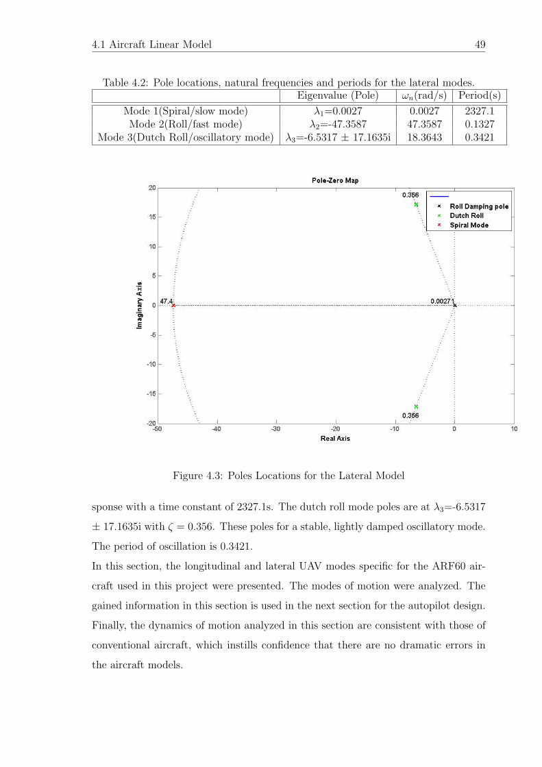
4.1 Aircraft Linear Model 49
Table 4.2: Pole locations, natural frequencies and periods for the lateral modes.Eigenvalue (Pole) ωn(rad/s) Period(s)
Mode 1(Spiral/slow mode) λ1=0.0027 0.0027 2327.1Mode 2(Roll/fast mode) λ2=-47.3587 47.3587 0.1327
Mode 3(Dutch Roll/oscillatory mode) λ3=-6.5317 ± 17.1635i 18.3643 0.3421
Figure 4.3: Poles Locations for the Lateral Model
sponse with a time constant of 2327.1s. The dutch roll mode poles are at λ3=-6.5317
± 17.1635i with ζ = 0.356. These poles for a stable, lightly damped oscillatory mode.
The period of oscillation is 0.3421.
In this section, the longitudinal and lateral UAV modes specific for the ARF60 air-
craft used in this project were presented. The modes of motion were analyzed. The
gained information in this section is used in the next section for the autopilot design.
Finally, the dynamics of motion analyzed in this section are consistent with those of
conventional aircraft, which instills confidence that there are no dramatic errors in
the aircraft models.

4.2 ARF60 UAV Autopilot design using Successive Loop Closure (SLC) 50
4.2 ARF60 UAV Autopilot design using Successive Loop Closure (SLC)
In this section, autopilot design steps are outlined. Furthermore, an overview of the
controller is given in Section 4.2.1. Finally, a detailed description of longitudinal and
lateral autopilots is explained in sections 4.2.2 and 4.2.3.
4.2.1 Autopilot Overview
The controller is designed so that the Aircraft is stable and performing the given spec-
ification. One simple approach to achieve this is to use open loop control. In such
control, the aircraft poles are merely cancelled by compensator zeros and the compen-
sator poles are used to define the desired aircraft dynamics. The problem with this
approach is that if the aircrafts dynamic model changes or the aircraft experiences
disturbances, the control system performance will deteriorate rapidly. Therefore,
feedback control is used to overcome open loop control problems. Feedback control
not only reduces the system sensitivity to modelling uncertainties, but also eliminates
disturbance and noise effects. Some Examples of disturbance types that affect aircraft
motion include wind disturbance, fuel level changes, changes in aircraft model due to
flight conditions and aeroelastic effects. The controller robustness is determined by
its ability to reduce system sensitivity to modelling errors.
The main task in controlling an aircraft is the control of the attitude since it
provides control over aircraft accelerations. For example, the bank angle of an aircraft
determines its centripetal acceleration. Direct control over the aircrafts acceleration is
desired because the stabilization effects integrate down into the velocity and position
states over time and thus leave only the reference velocity and position commands to
be regulated by outer control loops.
The aircraft controller involves three main controllers which are the stability
augmentation system (SAS) controller, the attitude stabilization (Autopilot) con-
troller and the trajectory tracking controller (Bernard Etkin, 1996).
The stability augmentation system provides artificial damping in order to sup-
press any high frequency aircraft dynamic. Furthermore, the attitude stabilizer reg-
ulates aircraft pitch and roll angles to control aircraft acceleration. Finally, the tra-
jectory tracker controls heading and altitude as an outer loop.

4.2 ARF60 UAV Autopilot design using Successive Loop Closure (SLC) 51
These control loops provide commands to the attitude controller and thus
deal with the kinematics of the aircraft. The advantage of this successive loop closure
design methodology is that once the attitude controllers have been implemented,
the trajectory controllers can be implemented in cascade because the outer control
algorithms are essentially independent of the inner ones.
Each of the three controller types is now discussed in more detail.
Stability Augmentation System (SAS) Controller
As stated previously, stability augmentation controller is responsible for suppressing
any high frequency aircraft dynamic by providing artificial damping.
An aircraft experiences high frequency during the short period mode, the dutch
roll mode and during the roll mode. The natural damping of such modes can be caused
by induced angles of incidence during angular rate disturbance which implies that the
damping is dependent on aircraft velocity and location of center of gravity. To alter
natural damping effect, an artificial damping is imposed by sensing aircraft angular
rates with gyroscopes. Then, the signals from gyroscopes are fed to their designated
actuators to augment aircraft natural damping.
In this thesis, both short period and dutch roll dampers are designed and
implemented. However, the artificial roll damper isn’t implemented since roll mode
is deeply damped with high frequency. The outer attitude control loops will reject
the wind gust disturbance.
Attitude Stabilization (Autopilot) Controller
Attitude stabilization controller regulates the aircraft pitch and roll angles and in
turn controls aircraft acceleration. One approach of implementing such a controller
is to use a Linear Quadratic Regulator (LQR) (Peddle, 2005). However, using such
approach isn’t practical since neither the aircraft model nor low cost sensors provide
high accurate data estimation and measurements. Typical examples of low cost sen-
sors include rate gyroscopes, infrared sensors and vision based systems. Although
rate gyroscopes work well in all environmental conditions, they have biases on the
order of a few tenths of a degree per second. Due to these poor biases, rate gyro-
scopes cannot be used alone to provide aircraft attitude measurements. Therefore,

4.2 ARF60 UAV Autopilot design using Successive Loop Closure (SLC) 52
rate gyroscopes are combined with a low cost set of accelerometers. In this case,
accelerometers provide acceptable attitude information on stationary platforms with
low frequency while rate gyroscopes provide good angular rate measurements at high
frequency. In other words, rate gyroscopes and accelerometers are used in a comple-
mentary filter where the rate gyroscopes give attitude information at high frequency
while accelerometers provide attitude information at low frequency. Although com-
bining rate gyros with accelerometers provide reasonable attitude information, it has
some drawbacks. During steady manoeuvres, it experiences adverse properties such
as constant turns or loops.
The solution to this problem is to use an estimator that takes measurements
from low cost rate gyroscopes, accelerometers and a variety of other sensors such
as a GPS receiver and a magnetometer. In such estimators, all aircraft states are
accurately estimated. however, it is computationally expensive and it is affected by
instruments failure. From the above discussion, it is obvious that determining aircraft
attitude based on sensors alone isn’t an easy task. However, if we can find the states
that are directly related to the aircraft attitude under common flight conditions and
then measure them using low cost sensors, the aircraft attitude can be indirectly
controlled. The designed controller is simple, requires low cost sensors and a small
computational power. Both the pitch and roll angle controllers are discussed below.
• Pitch Attitude Hold Consider the primary longitudinal state space model and
the climb rate equations described in Equation 4.6 and Equation 4.7, respec-
tively:
x = Ax+Bu (4.6)
h = Chx (4.7)
Both equations represent a set of five first order, linear differential equations
with 7 variables: u, w, q, θ, h, δe and δt . To have a unique solution of the
system, two more linearly independent equation are required. These equations
will be the control low equations that determine how the control variables are
calculated from different states. The change in airspeed is measured using a
differential pressure sensor while the climb rate is measured using an absolute
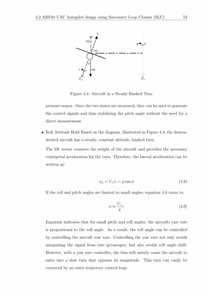
4.2 ARF60 UAV Autopilot design using Successive Loop Closure (SLC) 53
Figure 4.4: Aircraft in a Steady Banked Turn
pressure sensor. Once the two states are measured, they can be used to generate
the control signals and thus stabilizing the pitch angle without the need for a
direct measurement.
• Roll Attitude Hold Based on the diagram, illustrated in Figure 4.4, the demon-
strated aircraft has a steady, constant altitude, banked turn.
The lift vector counters the weight of the aircraft and provides the necessary
centripetal acceleration for the turn. Therefore, the lateral acceleration can be
written as:
aL = Uψ = g tanφ (4.8)
If the roll and pitch angles are limited to small angles; equation 4.8 turns to:
φ ≈ Ugr (4.9)
Equation indicates that for small pitch and roll angles, the aircrafts yaw rate
is proportional to the roll angle. As a result, the roll angle can be controlled
by controlling the aircraft yaw rate. Controlling the yaw rate not only avoids
integrating the signal from rate gyroscopes, but also avoids roll angle drift.
However, with a yaw rate controller, the bias will merely cause the aircraft to
enter into a slow turn that opposes its magnitude. This turn can easily be
corrected by an outer trajectory control loop.

4.2 ARF60 UAV Autopilot design using Successive Loop Closure (SLC) 54
Trajectory Tracking Controller
The trajectory tracking controllers are responsible for regulating the states of altitude
h, heading ψ and cross track error y.
These controllers are chosen because, together with the airspeed, climb rate
and yaw rate regulation capabilities of the attitude controllers, they make it possi-
ble for the autopilot to perform all conventional flight tasks. The altitude is easily
controlled by taking height measurement and feeding them to the climb rate con-
troller. The feedback is used to stabilize the extra integrator pole that the height
state adds to the system. The altitude measurement are obtained using an absolute
pressure sensor. Then, the heading and cross track error (guidance) controllers are
implemented by successive loop closure. A heading measurement can be fed to the
yaw rate controller to stabilize the extra integrator added to the system by the head-
ing state. The guidance controller can then be implemented by feeding a cross track
error measurement to the heading controller, to stabilize the single integrator added
to the system by the cross track error state. This successive loop closure technique
minimizes the amount of dynamic compensation required in implementing the two
lateral trajectory controllers. The heading and cross track error states can both be
measured using a low cost GPS receiver.
Summary of the Controllers
The stability augmentation systems, attitude stabilization and trajectory tracker con-
trollers discussed in the previous three sections, are divided into a longitudinal and
lateral set and summarized below.
• Longitudinal
1. Pitch Rate Damping.
2. Pitch attitude hold using elevator.
3. Airspeed hold using throttle.
4. Altitude hold using commanded pitch.
• Lateral
1. Roll Rate Damping.

4.2 ARF60 UAV Autopilot design using Successive Loop Closure (SLC) 55
2. Roll Attitude Hold.
3. Yaw Rate Damping.
The entire control system can be implemented using the following low cost
sensors,
• MIDG II Sensor: an Inertial Navigation System (INS) with Global Positioning
System (GPS)B.1.2.
• Differential Pressure Sensor B.1.4.
• Absolute Pressure Sensor B.1.3.
The following two sections provide the detailed design of the longitudinal and
lateral controllers as applied to the aircraft used in this project. All of the controllers
are designed in the continuous time domain. Then the controllers are converted to
the discrete domain using Tustin digitization method at a sample rate of 100Hz. This
rate was chosen as a convenient rate for implementation, well above the frequencies
of the aircrafts natural modes of motion. The discretization of these controllers is not
shown in this chapter. Successive loop closure was used for the autopilot design. The
basic idea that one loop is closed at a time. At each stage of the design, there is only
one gain to tune. Therefore, root locus techniques were used to design our autopilot
using successive loop closure (Randal W. Beard, 2007). Designing an autopilot using
these techniques requires linear models of the UAV dynamics for a number of trimmed
flight conditions. MATLAB was used to determine the trim conditions and derive
linear state-space models directly from the nonlinear UAV Simulink model. This
saved time and helped to validate the model. The functions provided by Simulink
Control Design allowed to visualize the behavior of the AUS ARF60 UAV in terms of
open-loop frequency and time responses. Figure 4.5 shows how the Lateral Autopilot
inner loops gains were tuned and validated using those tools.
4.2.2 Longitudinal Autopilot
The design and simulation of the aircrafts longitudinal controllers is considered in
this section. Each controller design begins with a discussion of the design approach
before the details of the controller are considered and the results verified by linear
and nonlinear simulation.
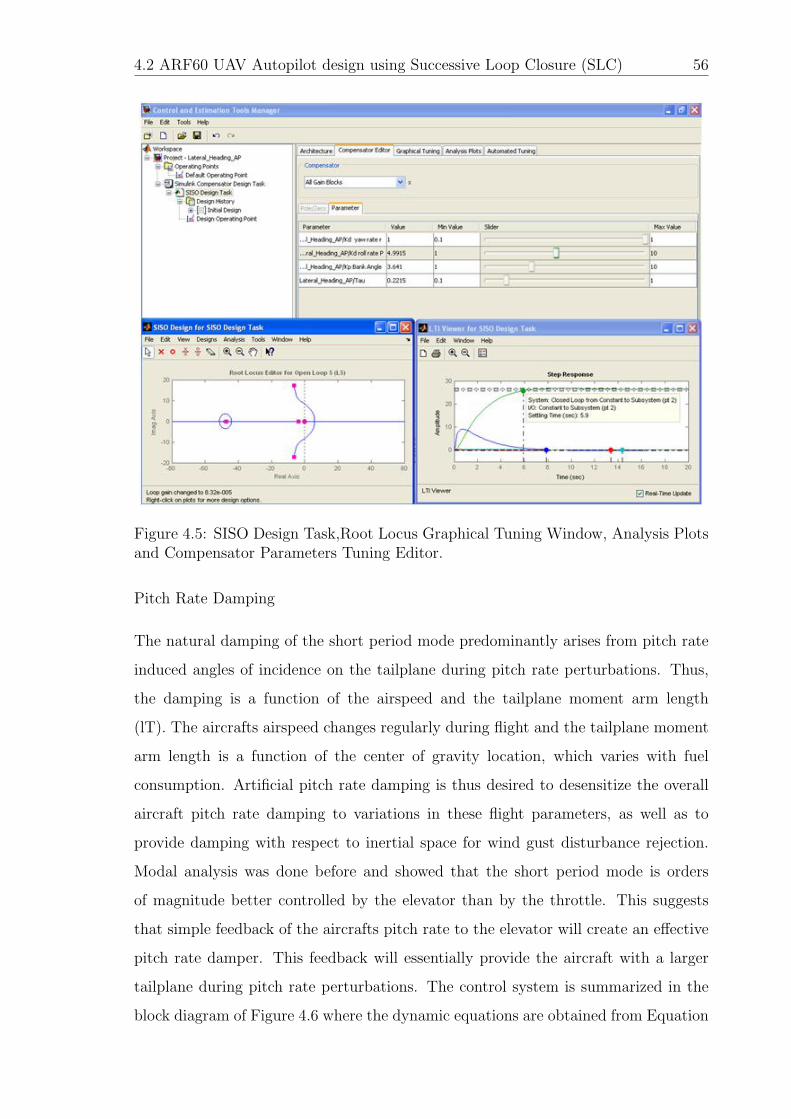
4.2 ARF60 UAV Autopilot design using Successive Loop Closure (SLC) 56
Figure 4.5: SISO Design Task,Root Locus Graphical Tuning Window, Analysis Plotsand Compensator Parameters Tuning Editor.
Pitch Rate Damping
The natural damping of the short period mode predominantly arises from pitch rate
induced angles of incidence on the tailplane during pitch rate perturbations. Thus,
the damping is a function of the airspeed and the tailplane moment arm length
(lT). The aircrafts airspeed changes regularly during flight and the tailplane moment
arm length is a function of the center of gravity location, which varies with fuel
consumption. Artificial pitch rate damping is thus desired to desensitize the overall
aircraft pitch rate damping to variations in these flight parameters, as well as to
provide damping with respect to inertial space for wind gust disturbance rejection.
Modal analysis was done before and showed that the short period mode is orders
of magnitude better controlled by the elevator than by the throttle. This suggests
that simple feedback of the aircrafts pitch rate to the elevator will create an effective
pitch rate damper. This feedback will essentially provide the aircraft with a larger
tailplane during pitch rate perturbations. The control system is summarized in the
block diagram of Figure 4.6 where the dynamic equations are obtained from Equation
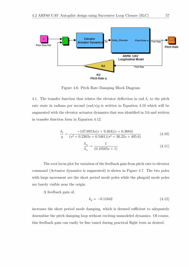
4.2 ARF60 UAV Autopilot design using Successive Loop Closure (SLC) 57
Figure 4.6: Pitch Rate Damping Block Diagram
4.1. The transfer function that relates the elevator deflection in rad δe to the pitch
rate state in radians per second (rad/s)q is written in Equation 4.10 which will be
augmented with the elevator actuator dynamics that was identified in 3.6 and written
in transfer function form in Equation 4.12.
δeq
=−147.6913s(s+ 9.404)(s+ 0.3084)
(s2 + 0.2303s+ 0.5461)(s2 + 36.22s+ 405.6)(4.10)
δea
δec
=1
(0.10505s+ 1)(4.11)
The root locus plot for variation of the feedback gain from pitch rate to elevator
command (Actuator dynamics is augmented) is shown in Figure 4.7. The two poles
with large movement are the short period mode poles while the phugoid mode poles
are barely visible near the origin.
A feedback gain of,
kq = −0.11642 (4.12)
increases the short period mode damping, which is deemed sufficient to adequately
desensitise the pitch damping loop without exciting unmodeled dynamics. Of course,
this feedback gain can easily be fine tuned during practical flight tests as desired.
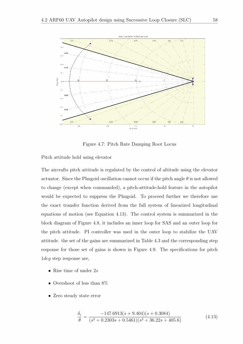
4.2 ARF60 UAV Autopilot design using Successive Loop Closure (SLC) 58
Figure 4.7: Pitch Rate Damping Root Locus
Pitch attitude hold using elevator
The aircrafts pitch attitude is regulated by the control of altitude using the elevator
actuator. Since the Phugoid oscillation cannot occur if the pitch angle θ is not allowed
to change (except when commanded), a pitch-attitude-hold feature in the autopilot
would be expected to suppress the Phugoid. To proceed further we therefore use
the exact transfer function derived from the full system of linearized longitudinal
equations of motion (see Equation 4.13). The control system is summarized in the
block diagram of Figure 4.8, it includes an inner loop for SAS and an outer loop for
the pitch attitude. PI controller was used in the outer loop to stabilize the UAV
attitude. the set of the gains are summarized in Table 4.3 and the corresponding step
response for those set of gains is shown in Figure 4.9. The specifications for pitch
1deg step response are,
• Rise time of under 2s
• Overshoot of less than 8%
• Zero steady state error
δeθ
=−147.6913(s+ 9.404)(s+ 0.3084)
(s2 + 0.2303s+ 0.5461)(s2 + 36.22s+ 405.6)(4.13)
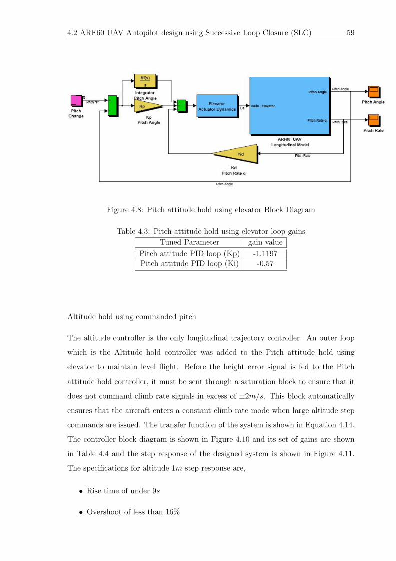
4.2 ARF60 UAV Autopilot design using Successive Loop Closure (SLC) 59
Figure 4.8: Pitch attitude hold using elevator Block Diagram
Table 4.3: Pitch attitude hold using elevator loop gains
Tuned Parameter gain value
Pitch attitude PID loop (Kp) -1.1197Pitch attitude PID loop (Ki) -0.57
Altitude hold using commanded pitch
The altitude controller is the only longitudinal trajectory controller. An outer loop
which is the Altitude hold controller was added to the Pitch attitude hold using
elevator to maintain level flight. Before the height error signal is fed to the Pitch
attitude hold controller, it must be sent through a saturation block to ensure that it
does not command climb rate signals in excess of ±2m/s. This block automatically
ensures that the aircraft enters a constant climb rate mode when large altitude step
commands are issued. The transfer function of the system is shown in Equation 4.14.
The controller block diagram is shown in Figure 4.10 and its set of gains are shown
in Table 4.4 and the step response of the designed system is shown in Figure 4.11.
The specifications for altitude 1m step response are,
• Rise time of under 9s
• Overshoot of less than 16%
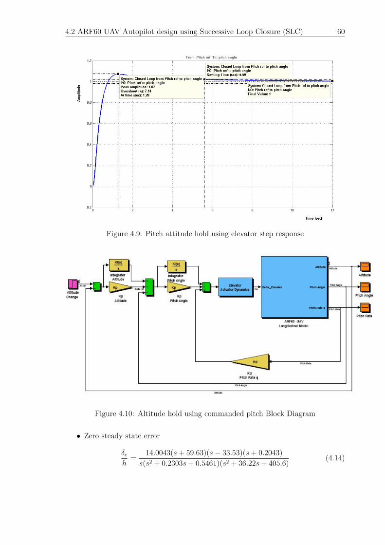
4.2 ARF60 UAV Autopilot design using Successive Loop Closure (SLC) 60
Figure 4.9: Pitch attitude hold using elevator step response
Figure 4.10: Altitude hold using commanded pitch Block Diagram
• Zero steady state error
δeh
=14.0043(s+ 59.63)(s− 33.53)(s+ 0.2043)
s(s2 + 0.2303s+ 0.5461)(s2 + 36.22s+ 405.6)(4.14)

4.2 ARF60 UAV Autopilot design using Successive Loop Closure (SLC) 61
Table 4.4: Altitude hold using commanded pitch loop gains
Tuned Parameter gain value
Altitude hold PID loop (Kp) 0.4744Altitude hold PID loop (Ki) 0.02224
Figure 4.11: Altitude hold using commanded pitch loop step response
Airspeed hold using throttle
Figure 4.12 is the block diagram of the control loop for the forward airspeed (u)
to maintain a constant speed along the flight path. the difference in flight speed is
used to produce proportional displacement of the engine throttle so that the speed
difference is reduced. The PI controller gains are listed in table 4.5. The step response
is shown in Figure 4.13. The specifications for airspeed 1m/s step response are,
• Rise time of under 2s
• Overshoot of less than 1%
• Zero steady state error
δtu
=51.5s(s2 + 36.22s+ 405.5)
(s2 + 0.2303s+ 0.5461)(s2 + 36.22s+ 405.6)(4.15)

4.2 ARF60 UAV Autopilot design using Successive Loop Closure (SLC) 62
Figure 4.12: Airspeed hold using throttle Block Diagram
Table 4.5: Airspeed hold using throttle loop gains
Tuned Parameter gain value
Airspeed hold PID loop (Kp) 0.02487Airspeed hold PID loop (Ki) 0.004564
4.2.3 Lateral Autopilot
The design and simulation of the aircrafts lateral controllers is considered in this
section. Each controller design begins with a discussion of the design approach before
the details of the controller are considered and the results verified by linear simulation.
Figure 4.13: Airspeed hold using throttle step response

4.2 ARF60 UAV Autopilot design using Successive Loop Closure (SLC) 63
Figure 4.14: ARF60 Longitudinal Autopilot Block Diagram
Figure 4.15: Roll Rate Damping Block Diagram
Roll Rate Damping
Closed loop control of roll rate (Figure 4.15)is used to reduce the variation of roll
performance with flight conditions.
Roll Attitude Hold
Feedback of the deviation of the roll angle to the ailerons (Figure 4.16)used to control
the aircraft’s roll angle thus the autopilot will hold the wings level.

4.2 ARF60 UAV Autopilot design using Successive Loop Closure (SLC) 64
Figure 4.16: Roll Attitude Hold Block Diagram
Dutch Roll Damper
Modal analysis showed that the natural damping of the dutch roll mode is low. Thus
a dutch roll damper is implemented in order to suppress the natural dynamics of the
dutch roll mode, desensitize the overall yaw damping to variation in flight parame-
ters and provide damping with respect to inertial space for wind gust disturbance.
Continuing along the same lines as the design of the pitch rate damper, the dutch
roll damper is implemented by feeding a yaw rate signal back to the rudder. The
rudder is used to provide the damping because it was shown by modal analysis to be
4 times more effective at controlling the dutch roll mode than the ailerons are. The
yaw rate signal must however, be high pass filtered before it is fed to the rudder so
that the damper does not counter constant turn rate motions. A secondary advan-
tage of the high pass filter is that it negates the bias effects of low cost rate gyroscopes.
The control system is summarized in the block diagram of Figure 4.17 where
the plant dynamics are taken from Equation 4.4 and shown in transfer function form
in Equation 4.16.The output matrix (C) is set to extract the yaw rate state in degrees
per second (deg/s). Note that the yaw rate signal moves through a washout filter
before being fed back to the rudder in a proportional fashion. Choosing the washout
filter cutoff frequency is an iterative process. However, it must be chosen low enough
to ensure the frequency of the dutch roll mode lies within its passband (without too
much phase error), but high enough so as not to interfere with constant turn rate
motions. With the natural frequency of the dutch roll mode at 18rad/s, a washout
filter cutoff frequency of 10rad/s is found to work well.
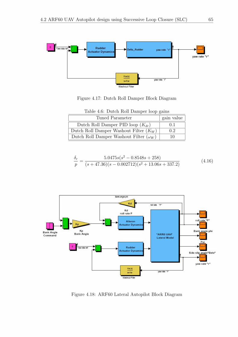
4.2 ARF60 UAV Autopilot design using Successive Loop Closure (SLC) 65
Figure 4.17: Dutch Roll Damper Block Diagram
Table 4.6: Dutch Roll Damper loop gains
Tuned Parameter gain value
Dutch Roll Damper PID loop (Kdr) 0.1Dutch Roll Damper Washout Filter (KW ) 0.2Dutch Roll Damper Washout Filter (ωW ) 10
δrp
=5.0475s(s2 − 0.8548s+ 258)
(s+ 47.36)(s− 0.002712)(s2 + 13.06s+ 337.2)(4.16)
Figure 4.18: ARF60 Lateral Autopilot Block Diagram

4.2 ARF60 UAV Autopilot design using Successive Loop Closure (SLC) 66
Figure 4.19: Path taken by the UAV When Entering a Curve using Feedback Guidance
4.2.4 Trajectory Tracker(Shortest Flight Algorithm in 3D)
In this thesis, the natural extension of feedback guidance strategy using band-bang
control strategy (Bhatt S. P., 2005) was used, simulated and implemented. The
algorithm contains straight lines and circular curves in each leg of the UAV mission.
Using this strategy, once the aircraft reaches a waypoint, it will start to turn until it
reaches the next waypoint and then fly straight to the next waypoint. However, there
are two circles where the aircraft can take; one circle is in the clockwise direction while
the other one is in the counterclockwise direction. The distance from the center of the
circular arc to the next waypoint determines which of the circles the aircraft chooses.
If the distance between the center of the circular arc and the next waypoint is smaller
than R (the minimum radius of the circular arc limited by the maximum turning rate
of the aircraft), the UAV will choose the circular arc whose center is farther from the
waypoint and vice versa. Figure 4.19(Hassan, 2006) represents the two circles that
the aircraft can maneuver from one way point to another. The heading of the aircraft
from its current position to the next waypoint is iteratively computed using Equation

4.2 ARF60 UAV Autopilot design using Successive Loop Closure (SLC) 67
Figure 4.20: Extension of the Feedback Guidance Strategy - Bidirectional
4.17. Then, the calculated heading is compared with the aircraft current heading.
If the heading error is within 10 degrees of the UAV current heading, the UAV will
bank in such a way that is proportional to the heading error, thus, reducing the error
before following a straight line to the next waypoint. Furthermore, the UAV will fly
a circular curve until it faces the next waypoint. Then, it will fly straight to the
waypoint if the next waypoint is more than 10 degrees of the UAV current heading.
Finally, if the heading error remains more than 10 degrees, the UAV will continue in
a circular path; otherwise, it will straighten.
Hp = arctan(YN − YC
XN −XC
) (4.17)
Where XN , YN are the coordinates of the next waypoint and XC , YC are the
instantaneous current coordinates. More Details descriptions of the feedback guidance
strategy using band-bang control strategy can be found in (Bhatt S. P., 2005).
Although feedback guidance strategy will allow the aircraft to reach its des-
tination, it doesn’t control the heading of the aircraft once it reaches its waypoint.
Therefore, feedback guidance strategy was extended to bidirectional Feedback Guid-
ance Strategy by (Hassan, 2006). Figure 4.20 shows the bidirectional Feedback Guid-
ance Strategy.
As indicated earlier, feedback Guidance Strategy is used to form a circle in
which the aircraft enters when travelling from points A to B to C. However, in bidi-
rectional Feedback Guidance Strategy, two circles are drawn; one is when the aircraft
travels from points A to B to C while the other one is when the aircraft travels from
points C to B to A. The switching point between the two circles is determined by the
point when the current direction of the aircraft is exactly 180 degrees (opposite) from

4.2 ARF60 UAV Autopilot design using Successive Loop Closure (SLC) 68
Figure 4.21: ARF60 Autopilot and Trajectory Tracker System Block Diagram
the theoretical current direction of the aircraft. At the switching point, the aircraft
will change its maneuvering from following the first circle to straight flight until in
intersects the other circle to follow the circular path again. The conditions where the
second switch occurs are summarized in Equations 4.18.
if0 ≤ θA < 180andθV = θA + 180 (4.18a)
elseifθA = 180andθV = 0 (4.18b)
elseif1800 ≤ θA < 360andθV = θA − 180 (4.18c)
Trajectory Tracker Results (Simulation)
Figures 4.22-4.24 show the plots of waypoint navigation using the extension of the
Feedback Guidance Strategy - Bidirectional ”simulation only” methods described
earlier. The results show that the aircraft reaches the desired waypoint ”dead on
target”. The reader must be given to understand that this is only a simulation
result where continuous updates of all the states necessary were available such as
position, heading, altitude, and all the other states necessary for the autopilots. These
parameters were available continuously, and were very precise, and they did not suffer

4.2 ARF60 UAV Autopilot design using Successive Loop Closure (SLC) 69
Figure 4.22: Four waypoints navigation results
from noise associated with sensing devices. Thus the results achieved can be described
as ideal. The Bang-Bang Trajectory Tracker with the SLC Autopilot completed the
mission with less than 500 seconds. Overall the SLC Autopilot performed as expected
and allowed the plane to bank more for a given bank reference command, and thus
take sharper and shorter turns.

4.2 ARF60 UAV Autopilot design using Successive Loop Closure (SLC) 70
Figure 4.23: Four waypoints navigation Map 2D
Figure 4.24: Four waypoints navigation plot 3D

Chapter 5
Control and Hardware Implementation
This chapter discusses the hardware and software involved in the avionics and ground
station. A block diagram overview of the system is shown in Figure 5.1.
The block diagram shows that the system is divided into two logical parts: the UAV
and the ground station. The UAV consists of a RC (Radio Controlled) receiver, a set
of servos and an avionics package developed. The ground station consists of a laptop
computer running the ground station software, an RF transceiver module and an RC
transmitter. The avionics package and ground station designs are discussed in more
detail. A summary of the system including a cost, power consumption and weight
analysis is presented in the final section.
Figure 5.1: AUS Avionics and Ground station Block Diagram

5.1 Signals, Hardware and Software 72
5.1 Signals, Hardware and Software
In order to provide some insight into the control system integration, the components
are briefly discussed.
5.1.1 Control Signals
Control signals are the method by which different components exchange information.
The two types of control signals used in this project are Remote Control (RC) Pulse
Width Modulation (PWM) controller area netork (CAN) and serial communications
using the RS-232 standard. RC Pulse Width Modulation Pulse Width Modulation
(PWM) is a technique commonly used to represent an analogue signal using digital
circuitry. Controller Area Network Controller Area Network (CAN or CAN-bus) is a
computer network protocol and bus standard designed to allow microcontrollers and
devices to communicate with each other and without a host computer.It was designed
specifically for automotive applications but is now also used in other areas. Serial
Communications Many devices communicate using an asynchronous serial communi-
cations port, ones in this project include the IMU.
5.1.2 Control Hardware
The control hardware is the hardware used to run the control system or assist in its
implementation.
dSPACE DS-1103
The dSPACE DS-1104 rapid prototyping platform is a real-time control target that
is extensively used in the construction and testing of control systems. The DS-1104
is an expansion card that sits on the host computers PCI bus and contains its own
PowerPC CPU and a Texas Instruments (TI) Digital Signal Processor (DSP). Matlab
Simulink models are compiled using a cross-C compiler and loaded to the DS-1104
platform. Usin gthe dSPACE software ControlDesk, variables and outputs from the
Simulink model are accessible via a Graphical User Interface (GUI). A dSPACE DS-
1104 breakout board is shown in Figure The DS-1104 hardware has eight Analogue
to Digital (A/D) converters, eight Digital the Analogue (D/A) converters, four PWM

5.1 Signals, Hardware and Software 73
outputs, one asynchronous serial port (either RS-232 or RS-422/485), two encoder
readers as well as a host of other inputs and outputs.
phyCORE-MPC555 Single Board Computer
A typical embedded system development process requires the evaluation of executable
specifications, design implementation by manually writing software, performance tun-
ing by trial and error, and testing using product prototypes. With this traditional
approach, errors are often found at or near the end of the development process where
they are costly and difficult to fix and can jeopardize the successful completion of
the project on time and within the stated budget. These problems become even
more critical when the target is a controller with a very intricate architecture such
as MPC555. This project demonstrates that the quality of any project depends not
merely on the end product, but more on the process involved in developing the prod-
uct. It reveals the solution to all such process-related problems by means of intro-
ducing model-based design. Model-based design clearly defines design specifications,
tests systems concepts and automatically develops code for rapid prototyping and
software development. The Mathworks provides evolution and adoption of model-
based design. Simulink is a software package provided by Mathworks for modeling,
simulating, and analyzing dynamic systems. Simulink provides a graphical user in-
terface (GUI) for building models as block diagrams, using drag and drop of blocks
from Simulink library. The most attractive feature is Automatic Code Generation
of developed model. Along with code reusability, an added advantage that Simulink
provides is that the code can be target specific. The advent of processors employing
newer technologies and even more complex architectures everyday dictates the need
of Target Specific Automatic code Generation. This relieves the design engineers
of having the full-fledged knowledge of architecture of target. The best example of
a ’next generation’ microcontroller is the MPC555, which is exclusively tailored for
automotive and industrial applications. MPC555 is a high performance modern au-
tomotive microcontroller with a very complex but reliable Power PC architecture.
When it comes to developing a system using MPC555, it is a time consuming and
tedious job to first study the entire architecture and then write the target specific C
/C++ code.
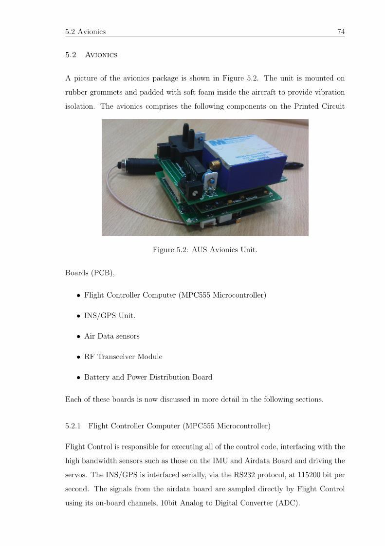
5.2 Avionics 74
5.2 Avionics
A picture of the avionics package is shown in Figure 5.2. The unit is mounted on
rubber grommets and padded with soft foam inside the aircraft to provide vibration
isolation. The avionics comprises the following components on the Printed Circuit
Figure 5.2: AUS Avionics Unit.
Boards (PCB),
• Flight Controller Computer (MPC555 Microcontroller)
• INS/GPS Unit.
• Air Data sensors
• RF Transceiver Module
• Battery and Power Distribution Board
Each of these boards is now discussed in more detail in the following sections.
5.2.1 Flight Controller Computer (MPC555 Microcontroller)
Flight Control is responsible for executing all of the control code, interfacing with the
high bandwidth sensors such as those on the IMU and Airdata Board and driving the
servos. The INS/GPS is interfaced serially, via the RS232 protocol, at 115200 bit per
second. The signals from the airdata board are sampled directly by Flight Control
using its on-board channels, 10bit Analog to Digital Converter (ADC).

5.2 Avionics 75
Figure 5.3: MIDG II:Inertial Navigation System (INS) with Global Positioning Sys-tem (GPS)
To allow Flight Control to switch between safety pilot and autopilot, the servos
are driven directly from the Microcontroller. This is done by re-routing the RC
receivers PWM signal, containing all of the servos position information. And capture
information is using the Time Processor Unit (TPU3). This allows allows the reading
of the input pin and measures an accumulation of time over a specified number of
periods. Manually driving the servos allows single control loops to be turned on at a
time, while the safety pilot controls the actuators not in use by the autopilot.
5.2.2 INS/GPS Unit
The MIDG II is an Inertial Navigation System (INS) with Global Positioning System
(GPS) contained in an incredibly small package. This INS GPS package is ideally
suited for any unmanned vehicle application that requires an inertial navigation so-
lution. The MIDG II INS/GPS package is specifically designed to be used with the
Microbotic Autopilot Platform, but can also be used with other autopilot packages
for primary instrumentation.
Message rates are configurable, and individual messages may be polled. All
data messages are time stamped with GPS time, and a One Pulse Per Second sig-
nal is available for time synchronization in the host computer. Operational mode
is selectable, including IMU only operation, vertical gyro simulation with magnetic
aiding, and full INS solution. MIDG is intended for use in applications requiring a full
state vector, including attitude, position, altitude, velocity, acceleration, and angular
rates. All measurements specifications are listed in Table 5.1. MIDG II INS/GPS
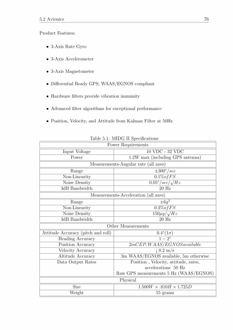
5.2 Avionics 76
Product Features:
• 3-Axis Rate Gyro
• 3-Axis Accelerometer
• 3-Axis Magnetometer
• Differential Ready GPS; WAAS/EGNOS compliant
• Hardware filters provide vibration immunity
• Advanced filter algorithms for exceptional performance
• Position, Velocity, and Attitude from Kalman Filter at 50Hz
Table 5.1: MIDG II Specifications
Power Requirements
Input Voltage 10 VDC - 32 VDCPower 1.2W max (including GPS antenna)
Measurements-Angular rate (all axes)
Range ±300/secNon-Linearity 0.1%ofFSNoise Density 0.05/sec/
√Hz
3dB Bandwidth 20 Hz
Measurements-Acceleration (all axes)
Range ±6g3
Non-Linearity 0.3%ofFSNoise Density 150µg/
√Hz
3dB Bandwidth 20 Hz
Other Measurements
Attitude Accuracy (pitch and roll) 0.4(1σ)Heading Accuracy 1− 2
Position Accuracy 2mCEP,WAAS/EGNOSavailableVelocity Accuracy ¡ 0.2 m/sAltitude Accuracy 3m WAAS/EGNOS available, 5m otherwiseData Output Rates Position , Velocity, attitude, rates,
accelerations 50 HzRaw GPS measurements 5 Hz (WAAS/EGNOS)
Physical
Size 1.500W × .810H × 1.725DWeight 55 grams

5.3 Ground Station Design 77
5.2.3 Battery and Power Distribution Board
The avionics power source is a, 9.6V, 3000mAh NiMH Battery Pack. The battery
is connected directly to the Power Distribution Board where it is routed as shown
in Figure 5.4. The servos and RC receiver are powered by an unregulated voltage
Figure 5.4: Block Diagram of Avionics Power Distribution
supply. This ensures that the servos always have access to a high current source
that may be needed in the event of a malfunctioning servo. If a standard regulator
were used during this event, it would either shut down or fail, rendering the aircraft
uncontrollable which we already faced in our first flight test, see section 7.1.2.
5.3 Ground Station Design
Figure 5.1 shows that the ground station is made up of a PC running the ground
station software, an RF communications module and a RC Transmitter. The RF
module provides a wireless link to the aircraft used for telemetry and communications
purposes. The ground station PC and the RF module communicate serially, via
the RS232 protocol, at 115200 baud. The ground station RF module is set up in
exactly the same way as the avionics RF module is. The only modification to the RC
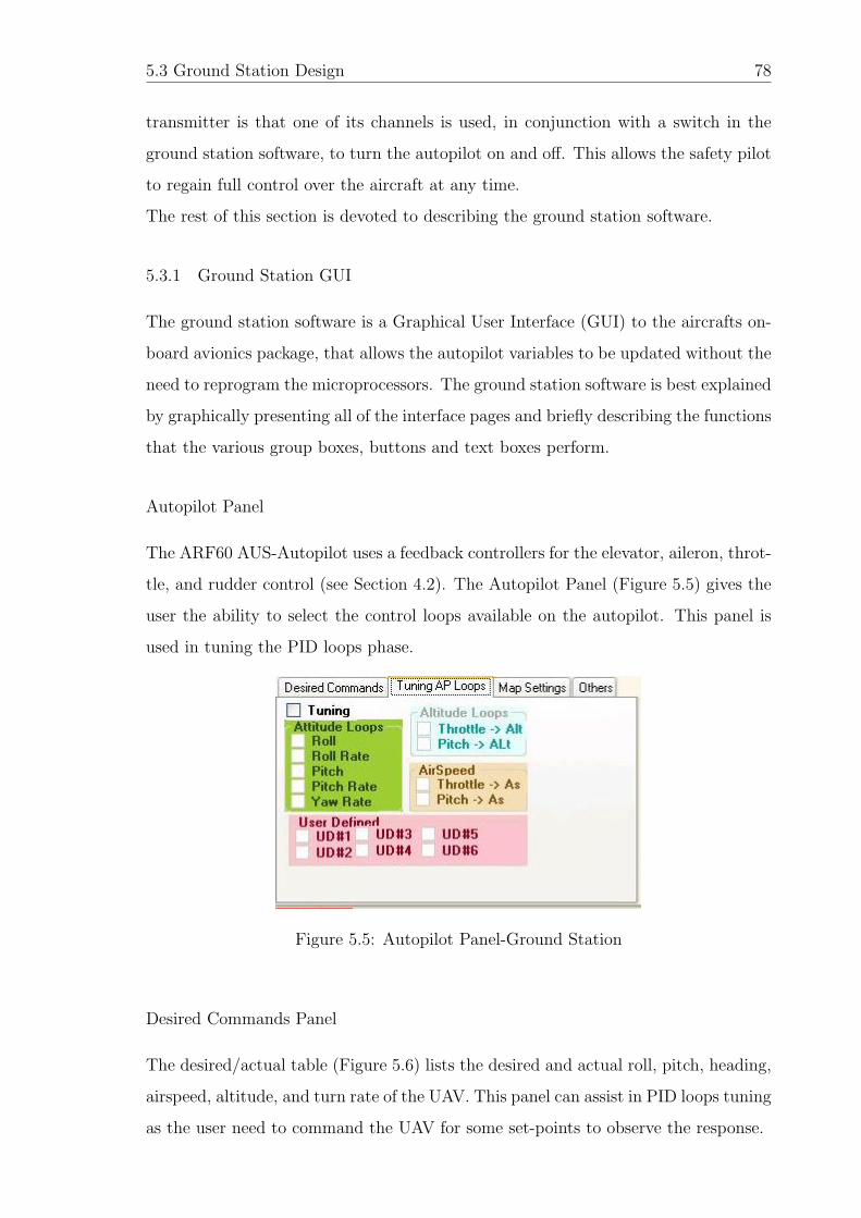
5.3 Ground Station Design 78
transmitter is that one of its channels is used, in conjunction with a switch in the
ground station software, to turn the autopilot on and off. This allows the safety pilot
to regain full control over the aircraft at any time.
The rest of this section is devoted to describing the ground station software.
5.3.1 Ground Station GUI
The ground station software is a Graphical User Interface (GUI) to the aircrafts on-
board avionics package, that allows the autopilot variables to be updated without the
need to reprogram the microprocessors. The ground station software is best explained
by graphically presenting all of the interface pages and briefly describing the functions
that the various group boxes, buttons and text boxes perform.
Autopilot Panel
The ARF60 AUS-Autopilot uses a feedback controllers for the elevator, aileron, throt-
tle, and rudder control (see Section 4.2). The Autopilot Panel (Figure 5.5) gives the
user the ability to select the control loops available on the autopilot. This panel is
used in tuning the PID loops phase.
Figure 5.5: Autopilot Panel-Ground Station
Desired Commands Panel
The desired/actual table (Figure 5.6) lists the desired and actual roll, pitch, heading,
airspeed, altitude, and turn rate of the UAV. This panel can assist in PID loops tuning
as the user need to command the UAV for some set-points to observe the response.

5.3 Ground Station Design 79
Figure 5.6: Desired Commands Panel-Ground Station
Actuators Monitoring Panel - For Sys ID
The Actuators Monitoring Panel (Figure 5.7) displays the actual position of the UAV
actuators as it is read from the servos potentiometer. This panel can be used to get
the user input commands for system identification purposes.
Figure 5.7: Actuators Monitoring Panel-Ground Station
States Monitoring Panel
The States Monitoring Panel is designed to give a visual reading of the orienta-
tion and status of the UAV and other avionics sensor data. There are two dif-
ferent views available, the gauges are used to show the most important states to
be monitored visually, while the less important ones are shown numerically. The
gauges that were used are the ActiveX Aircraft Instrumentation Library from GMS
(http : //www.globalmajic.com/).

5.3 Ground Station Design 80
Figure 5.8: States Monitoring Panel-Ground Station
Ground Station Map
The Map window is used to monitor the position and navigational status of the UAV
and to manage the flight plan. The Map displays the position of the UAV and its
waypoints. Figure 5.9 shows the map portion of the main Ground Station window.
Among other things, it shows a list of the current navigation waypoints as well as
indicating the waypoint that the aircraft is flying towards and the path of the aircraft.
It also allows waypoints to be added, edited and removed. The map can be customized
and configured using the Map Settings window (see Figure 5.10).
PID Loops Parameters Panel
The PID Parameters area is a table of the PID gains and limits used for control loops
tuning.
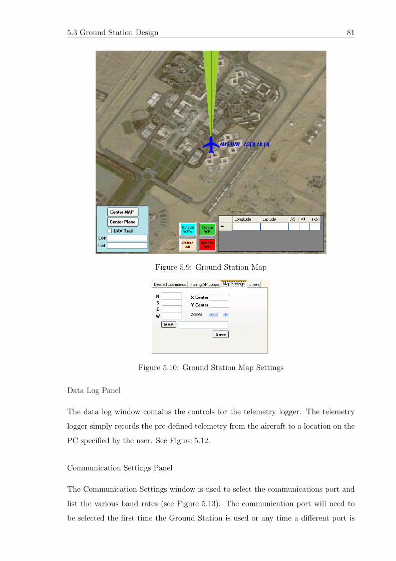
5.3 Ground Station Design 81
Figure 5.9: Ground Station Map
Figure 5.10: Ground Station Map Settings
Data Log Panel
The data log window contains the controls for the telemetry logger. The telemetry
logger simply records the pre-defined telemetry from the aircraft to a location on the
PC specified by the user. See Figure 5.12.
Communication Settings Panel
The Communication Settings window is used to select the communications port and
list the various baud rates (see Figure 5.13). The communication port will need to
be selected the first time the Ground Station is used or any time a different port is
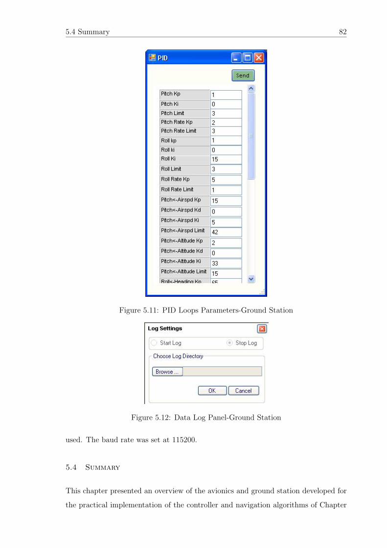
5.4 Summary 82
Figure 5.11: PID Loops Parameters-Ground Station
Figure 5.12: Data Log Panel-Ground Station
used. The baud rate was set at 115200.
5.4 Summary
This chapter presented an overview of the avionics and ground station developed for
the practical implementation of the controller and navigation algorithms of Chapter

5.4 Summary 83
Figure 5.13: Communication Settings Panel-Ground Station
4.
The cost, mass and power consumption summary of the avionics package is presented
in Table 5.2.
With the controller and navigation algorithms fully designed and the avionics and
ground station hardware and software ready, the autopilot is complete and ready for
flight tests.
Table 5.2: Cost, Mass and Power Consumption
Item Cost ($) Weight (Kg) Power (W)
MIDG INS/GPS 7750$ 0.051 1.2 MaxAirData Board 50$ 0.070MPC555 Board 519$ 0.1975Battery 9.6 V 59$ 0.432 -Battery 5 V 39$ 0.236 -Transceiver 149$ 0.0665 1 Max
Chapter 6
Hardware in the loop Simulation (HILS)
Simulation is an important phase that must be completed prior to any real world
practical testing. Unlike previously when mathematical models did not exist, excess
money was needed to test actual prototypes of real systems. A classic example is
the auto industry. In fact, there was no way of knowing before making the proto-
type or the real system if it would work as specified. If system were high powered
machinery that performed dangerous operation, failure of the equipment would often
be catastrophic and lead to losses in life. Currently modern systems are always by
default simulated in software before the actual prototype is tested. With the ac-
cumulation of knowledge, it is possible to acquire accurate mathematical models of
complete systems, and test them quickly due to advances in computing power. Thus
simulations reduce costs, and increases efficiency. Pure simulation is often used to
understand the behavior of a system, or to predict an outcome under different in-
ternal and external influences. Unfortunately although a pure simulation alone is
not enough to predict all possible outcomes due to the fact that not all practical
considerations may be taken into account. For most real systems, there are charac-
teristics that are unknown or too complex to model by pure simulation. That is why
nowadays Hardware in the Loop Simulation (HILS) testing is done. HILS is basically
a specific form of simulation, where a part of the mathematical model is replaced
by the actual hardware. Good system engineering practice would begin with a pure
simulation and as components become better defined with the aid of simulation, they
can be fabricated and replaced in the control loop. Once physical components are
added to the loop, un-modeled characteristics can be investigated, and controls can
be further refined. The use of HILS eliminates expensive and lengthy iterations in
machining and fabrication of parts, and speeds development towards a more efficient
design (Hadi, 2005).

6.1 Hardware in the Loop Simulation Development 85
Figure 6.1: Hardware-in-the-loop (HIL) simulation Setup
6.1 Hardware in the Loop Simulation Development
This section describes the details of developing a realistic simulation environment
based on Matlab/Simulink. A complete 6-DOF nonlinear aircraft model with a linear
approximation of the aerodynamic forces and moments is used to simulate realistic
dynamic behavior of the aircraft. The nonlinear aircraft model also involves the detail
modeling of subsystems such as sensors and actuators using experimental data. In
addition, the external pilot command input and the flight visualization enable the
simulation to be used as a virtual flight test. The actual autopilot hardware is placed
inside the simulation loop in order to test and validate both the hardware and the
on-board software. Four independent computer systems were used in the hardware-
in-the-loop (HIL) simulation as illustrated in Fig 6.1: the 6-DOF simulator, the
flight visualization computer, the autopilot micro-controller, and the ground station
computer console.
6.1.1 ARF60 UAV 6-DOF model simulator
A full 6-DOF nonlinear model for the ARF60 AUS-UAV was built in Matlab/Simulink
environment. The 12 states differential equations of motion in Eqs.2.4 - 2.8 are utilized
6.1 Hardware in the Loop Simulation Development 86
in conjunction with an approximation of the aerodynamic forces and moments via
component buildup. The stability and control derivatives are either obtained in the
manner as discussed in Section 3.4.1 or 3.4.2. The stability and control derivatives
from the geometry of the aircraft was chosen during the early phase of development,
however, once these derivatives have been identified experimentally, the identified
values are used for realistic simulation results. The output states from the simulator
are processed to emulate real sensors accounting for sensor latency, random walk
bias, and measurement noise. After digitized according to the word size of the micro-
controller (10 bit, 1024 steps), the sensor values are transmitted to the autopilot via
a serial communication. In a similar manner, the navigation states are processed
for data latency and measurement noise and encapsulated in a binary GPS packet
identical to the actual GPS sensor output. This packet is also transmitted to the
autopilot at an update rate of (50 Hz) via the serial communication baud rate of
(115200 bits per second). In the HILS environment, the autopilot functions identically
as in a real flight test, while computing control commands to each control actuator.
These commands are sent back to the 6-DOF simulator in order to drive the actuator
model of the control surface. Each control surface was modeled as a first order system
with saturation limit, whose parameters were identified experimentally. Consequently,
a simulation loop is formed between the 6-DOF simulator (software) and the autopilot
(hardware) exchanging the simulated data back and forth.
6.1.2 R/C transmitter
An R/C transmitter is connected to the 6-DOF simulator for recording remote pilot
stick commands: Four channels for control surface commands (δa, δe, δr and δt) and
auxiliary commands for toggling between autonomous control mode and remote pilot
mode. The remote pilot stick commands can override the autopilot control command
at any time by switching the commands to the actuator models at users choice. In
this case, a simulation for an open loop maneuver can be conducted along the remote
pilot input to validate the dynamic characteristic of the aircraft model. In order to
visualize the simulation, we adopted the use of FlighGear (v1.9.1, 2009), an open
source flight simulator for a visualization tool. The FlightGear is a flight simulator
framework, which has been widely used in various research environment. Although
it provides a total simulation environment in conjunction with the internal flight
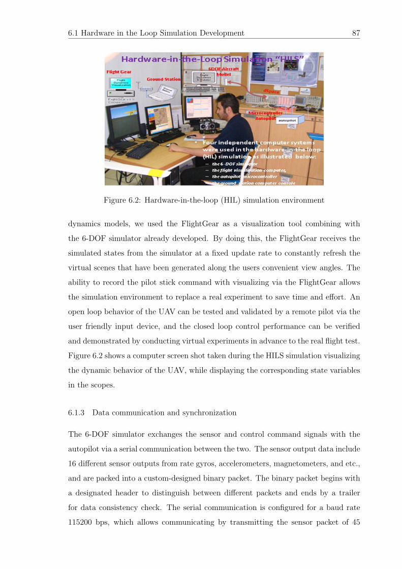
6.1 Hardware in the Loop Simulation Development 87
Figure 6.2: Hardware-in-the-loop (HIL) simulation environment
dynamics models, we used the FlightGear as a visualization tool combining with
the 6-DOF simulator already developed. By doing this, the FlightGear receives the
simulated states from the simulator at a fixed update rate to constantly refresh the
virtual scenes that have been generated along the users convenient view angles. The
ability to record the pilot stick command with visualizing via the FlightGear allows
the simulation environment to replace a real experiment to save time and effort. An
open loop behavior of the UAV can be tested and validated by a remote pilot via the
user friendly input device, and the closed loop control performance can be verified
and demonstrated by conducting virtual experiments in advance to the real flight test.
Figure 6.2 shows a computer screen shot taken during the HILS simulation visualizing
the dynamic behavior of the UAV, while displaying the corresponding state variables
in the scopes.
6.1.3 Data communication and synchronization
The 6-DOF simulator exchanges the sensor and control command signals with the
autopilot via a serial communication between the two. The sensor output data include
16 different sensor outputs from rate gyros, accelerometers, magnetometers, and etc.,
and are packed into a custom-designed binary packet. The binary packet begins with
a designated header to distinguish between different packets and ends by a trailer
for data consistency check. The serial communication is configured for a baud rate
115200 bps, which allows communicating by transmitting the sensor packet of 45
6.1 Hardware in the Loop Simulation Development 88
bytes at 50 Hz as well as the GPS navigation solution packet of 35 bytes at 50 Hz
update rate. The control command data from the autopilot are composed of four
PWM commands for each actuator, resulting in a binary packet of 36 bytes in length
associated with header and trailer to be transmitted at 50 Hz update rate. The HILS
bridge shown in Figure 6.1 was then incorporated into the 6-DOF Simulink model
to handle the bidirectional communication with a help of the serial communication
block toolbox (Leonardo, ). In addition, a dedicated S-function block is utilized to
send simulated output to the FlightGear (v1.9.1, 2009). Because the multiple systems
are involved in the HILS simulation, it is all important to keep the execution timing
among these systems properly synchronized during the entire simulation period for
data compatibility among them. Besides, a real-time execution is necessary for the
simulation to be in accord with the pilot input and the visualization at correct time
step. Although the 6-DOF simulator was written in a Simulink model running at
non real-time, a real time execution was accomplished by utilizing the Realtime block
toolbox and dSPACE enviroment (dSPACE, ). This toolbox (dSPACE) makes control
engineers lives easier with real-time tools for rapid control prototyping, production
code generation, and hardware-in-the-loop simulation. For a real time simulation,
the basic simulation time step of the 6-DOF simulator is carefully chosen at 100 [Hz]
taking into consideration both the computational overhead and the faithful simulation
results for accurate dynamic characteristics of the UAV. A different sampling rate at
50 [Hz] was utilized for the serial communication block and the FlightGear S-function
block. The synchronization of the data was implicitly dealt with in a manner that
the main simulation loop of the 6-DOF simulator polls each communication block
at a fixed interval during the simulation, whereas the autopilot and the FlightGear
receive the packets passively.
6.1.4 HILS Summary
A hardware-in-the-loop simulation environment has been built to validate hardware
and software development of the autopilot for a small UAV. A full 6-DOF nonlin-
ear dynamic model has been used in conjunction with the linear approximation of
the aerodynamic forces and moments. A batch parameter identification method has
been used to determine the stability and control derivatives of the UAV using flight
test data. Detailed models for the sensors and actuators were incorporated in the
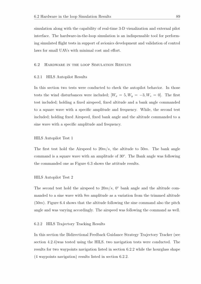
6.2 Hardware in the loop Simulation Results 89
simulation along with the capability of real-time 3-D visualization and external pilot
interface. The hardware-in-the-loop simulation is an indispensable tool for perform-
ing simulated flight tests in support of avionics development and validation of control
laws for small UAVs with minimal cost and effort.
6.2 Hardware in the loop Simulation Results
6.2.1 HILS Autopilot Results
In this section two tests were conducted to check the autopilot behavior. In those
tests the wind disturbances were included; [Wx = 5,Wy = −3,Wz = 0]. The first
test included; holding a fixed airspeed, fixed altitude and a bank angle commanded
to a square wave with a specific amplitude and frequency. While, the second test
included; holding fixed Airspeed, fixed bank angle and the altitude commanded to a
sine wave with a specific amplitude and frequency.
HILS Autopilot Test 1
The first test hold the Airspeed to 20m/s, the altitude to 50m. The bank angle
command is a square wave with an amplitude of 30. The Bank angle was following
the commanded one as Figure 6.3 shows the attitude results.
HILS Autopilot Test 2
The second test hold the airspeed to 20m/s, 0 bank angle and the altitude com-
manded to a sine wave with 8m amplitude as a variation from the trimmed altitude
(50m). Figure 6.4 shows that the altitude following the sine command also the pitch
angle and was varying accordingly. The airspeed was following the command as well.
6.2.2 HILS Trajectory Tracking Results
In this section the Bidirectional Feedback Guidance Strategy Trajectory Tracker (see
section 4.2.4)was tested using the HILS. two navigation tests were conducted. The
results for two waypoints navigation listed in section 6.2.2 while the hourglass shape
(4 waypoints navigation) results listed in section 6.2.2.

6.2 Hardware in the loop Simulation Results 90
Figure 6.3: HILS Autopilot Test 1 -Attitudes
Figure 6.4: HILS Autopilot Test 2 - States Results
HILS Trajectory Tracking Results-2WP Navigation
Two waypoints were feeded to the trajectory tracker to follow. Figure 6.5 show the
2D plot for the navigation between 2 waypoints with a distance of 500m in between.
The 3D plot and the map for the trajectory are shown in Figures ?? and 6.7. Figure
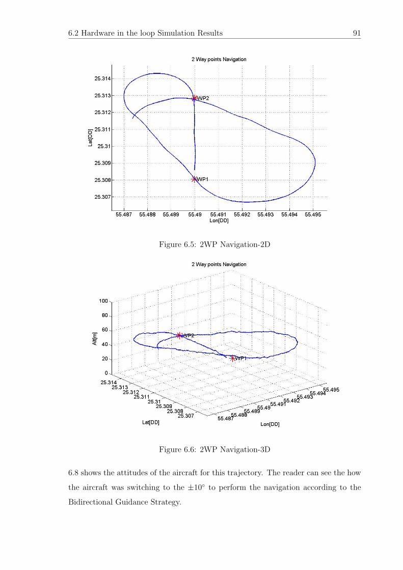
6.2 Hardware in the loop Simulation Results 91
Figure 6.5: 2WP Navigation-2D
Figure 6.6: 2WP Navigation-3D
6.8 shows the attitudes of the aircraft for this trajectory. The reader can see the how
the aircraft was switching to the ±10 to perform the navigation according to the
Bidirectional Guidance Strategy.
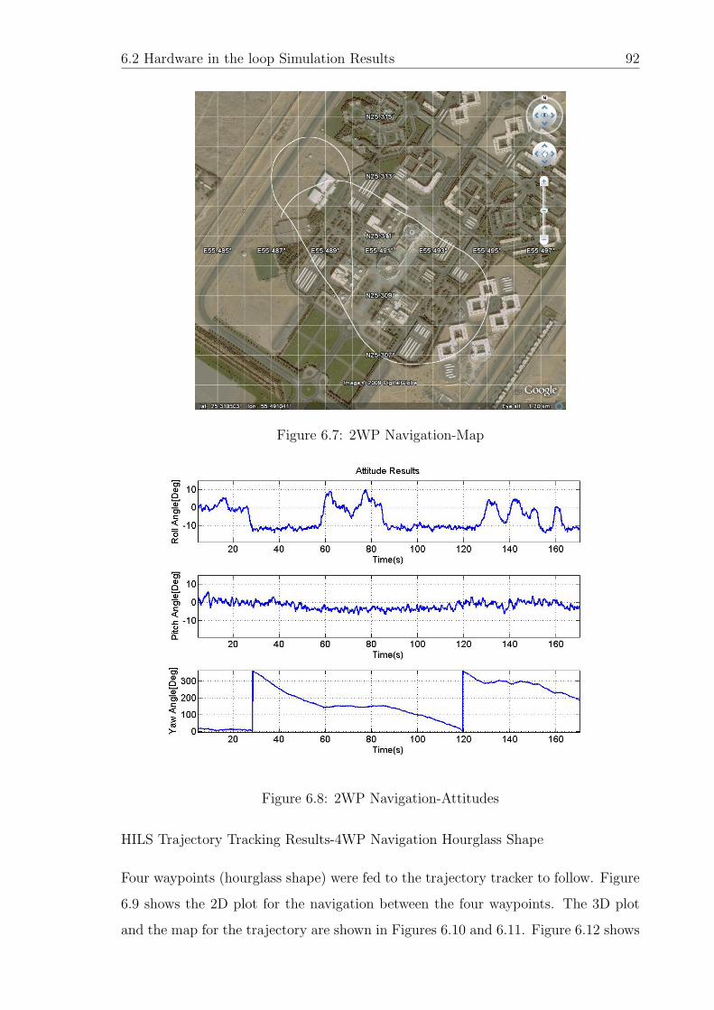
6.2 Hardware in the loop Simulation Results 92
Figure 6.7: 2WP Navigation-Map
Figure 6.8: 2WP Navigation-Attitudes
HILS Trajectory Tracking Results-4WP Navigation Hourglass Shape
Four waypoints (hourglass shape) were fed to the trajectory tracker to follow. Figure
6.9 shows the 2D plot for the navigation between the four waypoints. The 3D plot
and the map for the trajectory are shown in Figures 6.10 and 6.11. Figure 6.12 shows
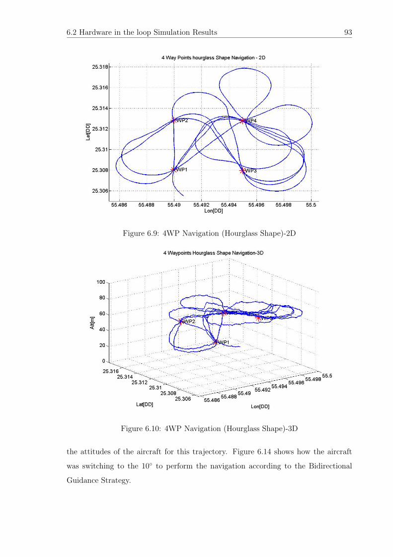
6.2 Hardware in the loop Simulation Results 93
Figure 6.9: 4WP Navigation (Hourglass Shape)-2D
Figure 6.10: 4WP Navigation (Hourglass Shape)-3D
the attitudes of the aircraft for this trajectory. Figure 6.14 shows how the aircraft
was switching to the 10 to perform the navigation according to the Bidirectional
Guidance Strategy.
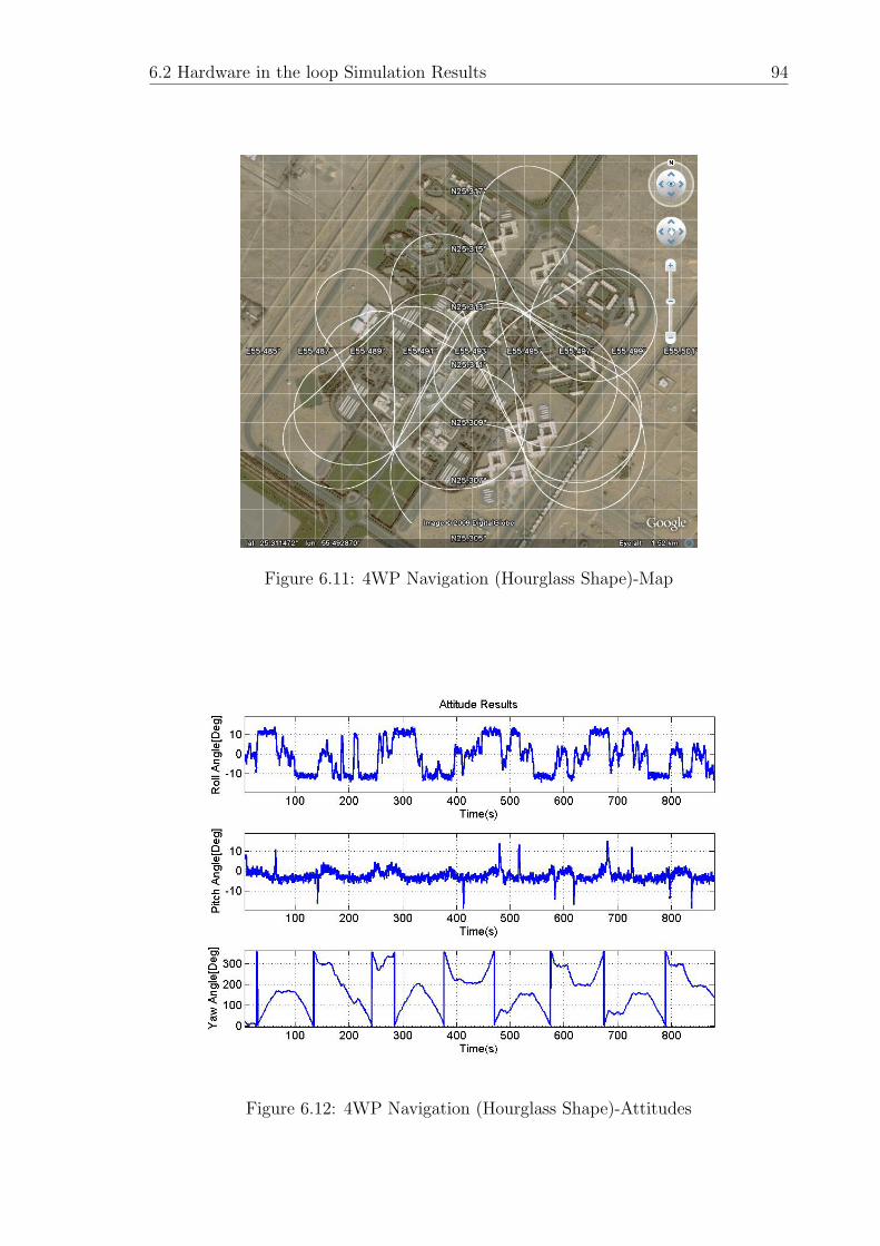
6.2 Hardware in the loop Simulation Results 94
Figure 6.11: 4WP Navigation (Hourglass Shape)-Map
Figure 6.12: 4WP Navigation (Hourglass Shape)-Attitudes

Chapter 7
Flight Tests Results and Autopilot Tuning
This chapter outlines a 3rd party autopilot mounting and tuning. It begins by intro-
ducing the kestrel autopilot, a commercial off the shelf autopilot. Then, it proceeds
to the discussion of the flight testing results in terms of loops tuning and trajectory
tracking. Furthermore, the designed autopilot for the ARF60 AUS-UAV is discussed
in terms of the utilized hardware, tuning steps and trajectory tracking results. Fi-
nally, we concluded by benchmarking the ARF60 AUS-UAV autopilot with the kestrel
autopilot in terms of accuracy.
7.1 Kestrel Autopilot Overview
Kestrel autopilot, shown in Figure 7.1, was integrated in the ARF60 aircraft. This
autopilot is used to bench mark the designed autopilot at AUS and compare their
capabilities. A variety of sensors were used to provide the necessary data for au-
tonomous control of the UAV. These sensors include three magnetometers, three
rate gyros, three accelerometers, a differential and absolute pressure sensors, a GPS
sensor, and three temperature sensors. The Kestrel uses an onboard 8-bit 29MHz
processor to handle all the sensor data and run the necessary code for controlling
the aircraft via four servo ports on the actual Kestrel unit and eight additional servo
ports on a servo expansion board. The Kestrel uses a Maxstream 9XTend 900MHz
1000 mW wireless modem to communicate with the ground station; this connects
to the bottom face of the autopilots PCB board through the modem header. The
two components were then secured together with heat shrink tubing to prevent any
separation during normal operation. Furthermore, the Kestrel autopilot can perform
GPS navigation using waypoints uploaded to the autopilot from the ground station.
Figures 7.2 and 7.3 show the block diagram of the Kestrel autopilot and its main
components respectively.

7.1 Kestrel Autopilot Overview 96
Figure 7.1: Kestrel Autopilot
Figure 7.2: Kestrel Autopilot Diagram
7.1.1 Mounting Kestrel Autopilot on the ARF60 UAV
The autopilot, pitot static tube, GPS, and radio modem antenna were installed cor-
rectly in the ARF60 aircraft.
The autopilot was installed flat with spacers of 15 mm long from the aircraft
fuselage bottom (see Figure 7.4). Then, set of rubbers were used to decrease the
effect of the engine vibration, Figures 7.5 and 7.6 shows the how the rubbers were
mounted. An aluminum box was designed to house the autopilot in order to protect

7.1 Kestrel Autopilot Overview 97
Figure 7.3: Kestrel Autopilot Block Diagram
it in the event of a crash or hard landing. Figure 7.7 shows the autopilot installed in
the airframe inside the aluminume box.
Figure 7.4: Kestrel Autopilot with spacers
The GPS receiver is one of the most important autopilot sensors. Without
GPS reception, the aircraft cannot estimate its position, ground speed, or ground
track. Loss of GPS reception during flight can result in the loss of the aircraft, as the
autopilot cannot navigate. The GPS unit was mounted in such a way that the antenna

7.1 Kestrel Autopilot Overview 98
Figure 7.5: Kestrel Autopilot isolation from inside
Figure 7.6: Kestrel Autopilot isolation from outside
has a clear view of the sky. To significantly improve the GPS receiver performance a
ground plane 2× 2 inches was added under the antenna. Figure 7.8 shows the GPS
location on the aircraft.
The digital radio modem is a key element of the autopilot system. Without
the digital modem, there is no way to communicate with the aircraft during flight.
Maxstream 9XTend 900MHz with 115k baud rate TTL level digital modem was used
with the autopilot. This modem is lightweight and, with a decent antenna, can

7.1 Kestrel Autopilot Overview 99
Figure 7.7: Kestrel Autopilot inside the Aluminume box
Figure 7.8: GPS Location on the aircraft
achieve ranges greater than 10 kilometers. A simple lightweight antenna was mounted
vertically on the ARF60 aircraft fuselage. The antenna location is shown in Figure
7.9.
The pitot system is critical for correct airspeed and altitude readings. The
airspeed measurement is derived from a differential pressure sensor that measures the
difference between static pressure and the pressure from the forward airspeed. The
pressure port on the differential pressure sensor was connected using silicon fuel tubing
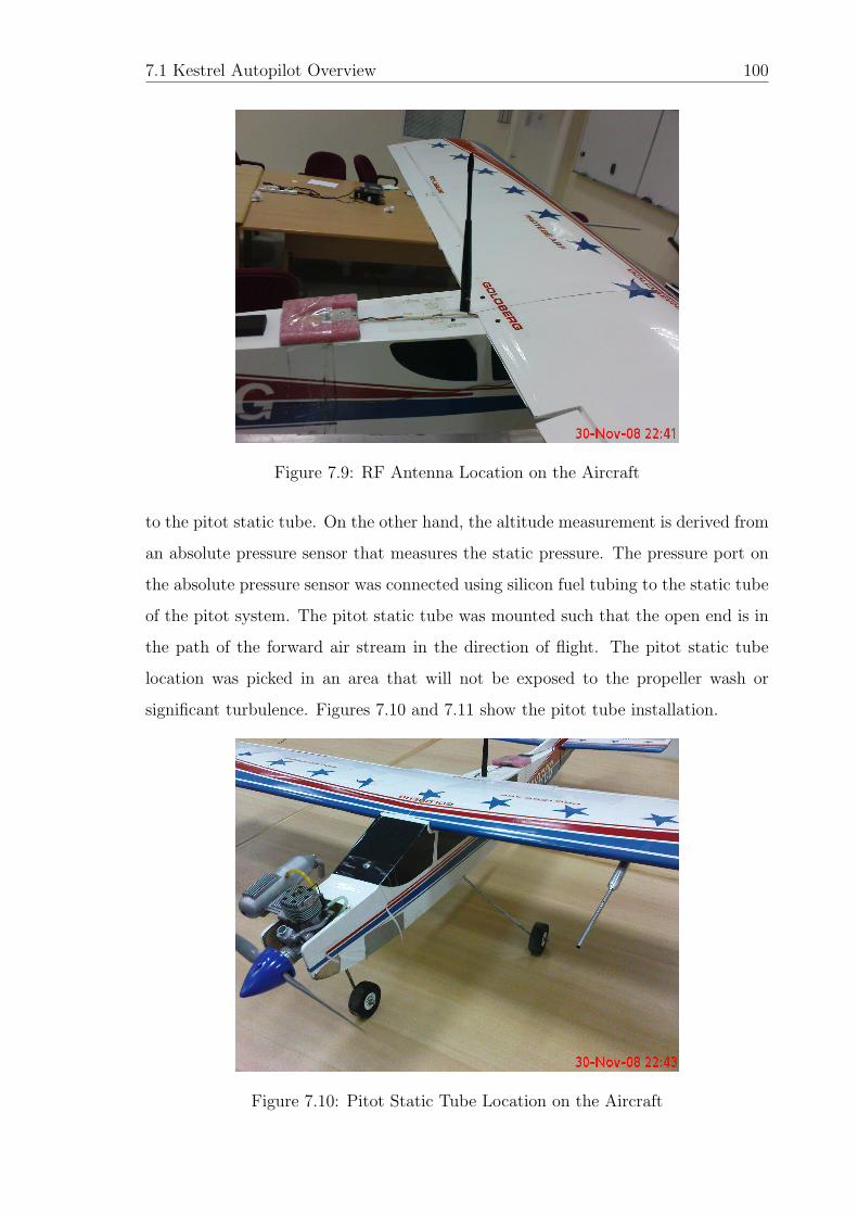
7.1 Kestrel Autopilot Overview 100
Figure 7.9: RF Antenna Location on the Aircraft
to the pitot static tube. On the other hand, the altitude measurement is derived from
an absolute pressure sensor that measures the static pressure. The pressure port on
the absolute pressure sensor was connected using silicon fuel tubing to the static tube
of the pitot system. The pitot static tube was mounted such that the open end is in
the path of the forward air stream in the direction of flight. The pitot static tube
location was picked in an area that will not be exposed to the propeller wash or
significant turbulence. Figures 7.10 and 7.11 show the pitot tube installation.
Figure 7.10: Pitot Static Tube Location on the Aircraft
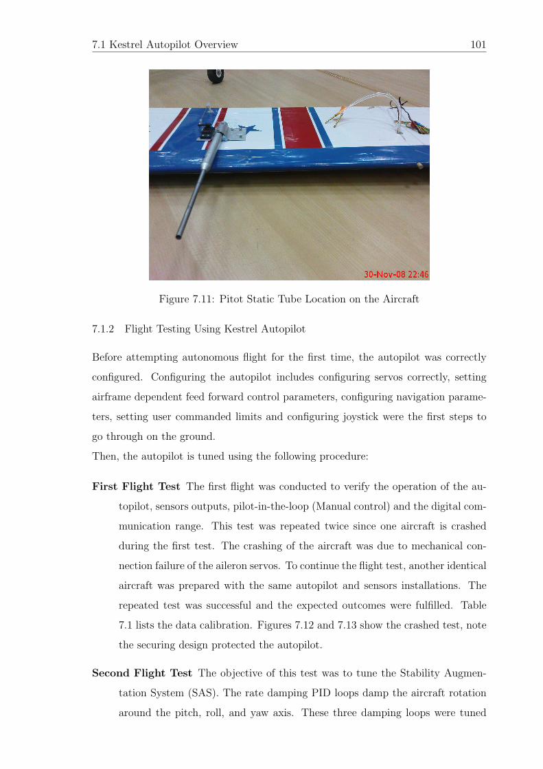
7.1 Kestrel Autopilot Overview 101
Figure 7.11: Pitot Static Tube Location on the Aircraft
7.1.2 Flight Testing Using Kestrel Autopilot
Before attempting autonomous flight for the first time, the autopilot was correctly
configured. Configuring the autopilot includes configuring servos correctly, setting
airframe dependent feed forward control parameters, configuring navigation parame-
ters, setting user commanded limits and configuring joystick were the first steps to
go through on the ground.
Then, the autopilot is tuned using the following procedure:
First Flight Test The first flight was conducted to verify the operation of the au-
topilot, sensors outputs, pilot-in-the-loop (Manual control) and the digital com-
munication range. This test was repeated twice since one aircraft is crashed
during the first test. The crashing of the aircraft was due to mechanical con-
nection failure of the aileron servos. To continue the flight test, another identical
aircraft was prepared with the same autopilot and sensors installations. The
repeated test was successful and the expected outcomes were fulfilled. Table
7.1 lists the data calibration. Figures 7.12 and 7.13 show the crashed test, note
the securing design protected the autopilot.
Second Flight Test The objective of this test was to tune the Stability Augmen-
tation System (SAS). The rate damping PID loops damp the aircraft rotation
around the pitch, roll, and yaw axis. These three damping loops were tuned
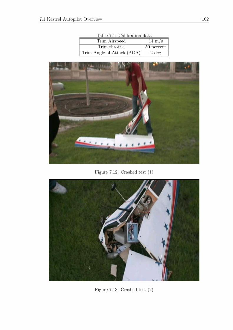
7.1 Kestrel Autopilot Overview 102
Table 7.1: Calibration dataTrim Airspeed 14 m/sTrim throttle 50 percent
Trim Angle of Attack (AOA) 2 deg
Figure 7.12: Crashed test (1)
Figure 7.13: Crashed test (2)
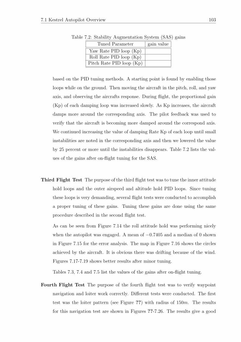
7.1 Kestrel Autopilot Overview 103
Table 7.2: Stability Augmentation System (SAS) gains
Tuned Parameter gain value
Yaw Rate PID loop (Kp)Roll Rate PID loop (Kp)Pitch Rate PID loop (Kp)
based on the PID tuning methods. A starting point is found by enabling those
loops while on the ground. Then moving the aircraft in the pitch, roll, and yaw
axis, and observing the aircrafts response. During flight, the proportional gain
(Kp) of each damping loop was increased slowly. As Kp increases, the aircraft
damps more around the corresponding axis. The pilot feedback was used to
verify that the aircraft is becoming more damped around the correspond axis.
We continued increasing the value of damping Rate Kp of each loop until small
instabilities are noted in the corresponding axis and then we lowered the value
by 25 percent or more until the instabilities disappears. Table 7.2 lists the val-
ues of the gains after on-flight tuning for the SAS.
Third Flight Test The purpose of the third flight test was to tune the inner attitude
hold loops and the outer airspeed and altitude hold PID loops. Since tuning
these loops is very demanding, several flight tests were conducted to accomplish
a proper tuning of these gains. Tuning these gains are done using the same
procedure described in the second flight test.
As can be seen from Figure 7.14 the roll attitude hold was performing nicely
when the autopilot was engaged. A mean of −0.7405 and a median of 0 shown
in Figure 7.15 for the error analysis. The map in Figure 7.16 shows the circles
achieved by the aircraft. It is obvious there was drifting because of the wind.
Figures 7.17-7.19 shows better results after minor tuning.
Tables 7.3, 7.4 and 7.5 list the values of the gains after on-flight tuning.
Fourth Flight Test The purpose of the fourth flight test was to verify waypoint
navigation and loiter work correctly. Different tests were conducted. The first
test was the loiter pattern (see Figure ??) with radius of 150m. The results
for this navigation test are shown in Figures ??-7.26. The results give a good

7.1 Kestrel Autopilot Overview 104
Figure 7.14: Roll Hold Test1
Figure 7.15: Roll Hold Test1 Error Analysis
impression about the tuning that has been done as the commanded signals were
followed nicely.

7.1 Kestrel Autopilot Overview 105
Figure 7.16: Roll Hold Test1 Map
Figure 7.17: Roll Hold Test2

7.1 Kestrel Autopilot Overview 106
Figure 7.18: Roll Hold Test2 Error Analysis
Figure 7.19: Roll Hold Test2 Map
Another loiter test with radius of 100m is conducted with the results shown in

7.1 Kestrel Autopilot Overview 107
Figure 7.20: Pitch Hold Test
Figure 7.21: Airspeed Hold Test
Figures ??-??.
Four waypoints trajectory, shaped a square pattern (see Figure 7.27), was the
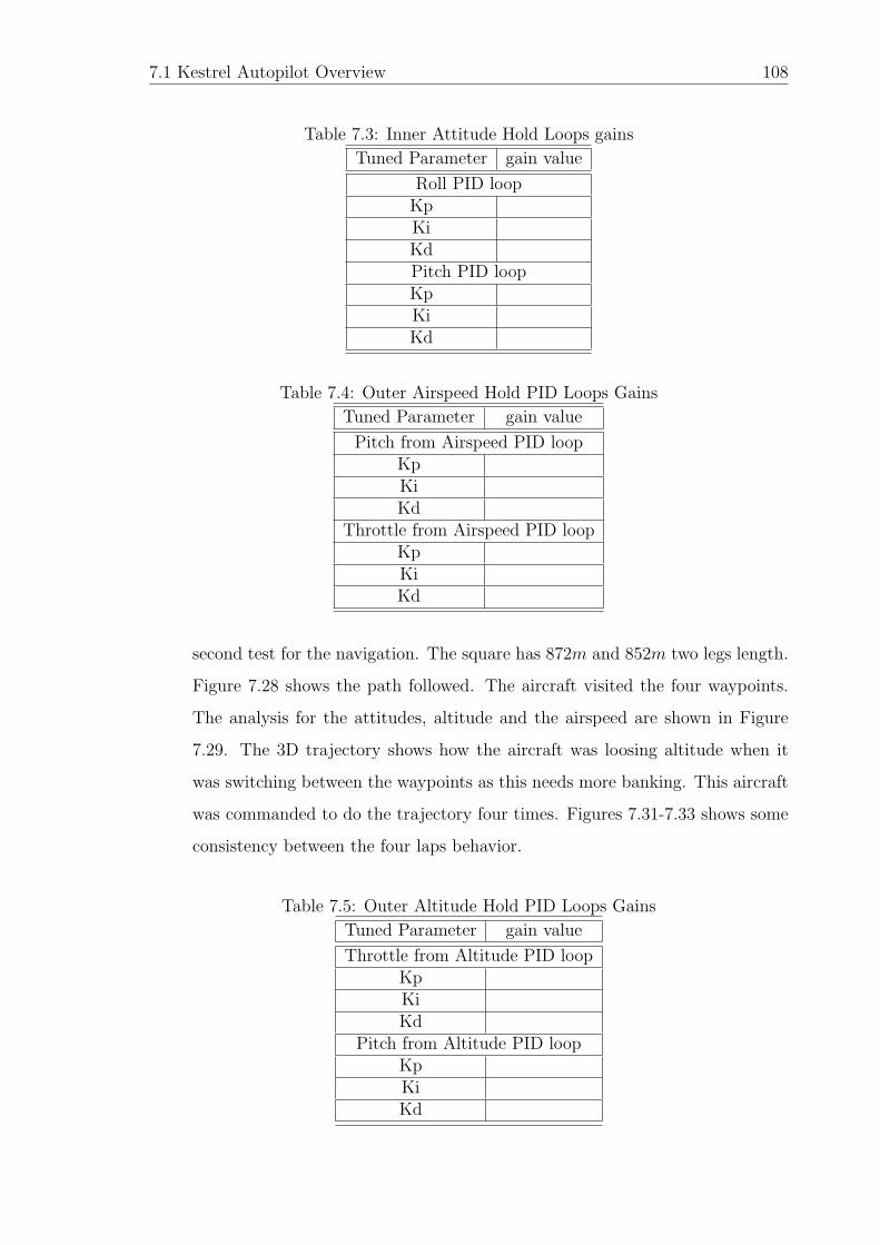
7.1 Kestrel Autopilot Overview 108
Table 7.3: Inner Attitude Hold Loops gains
Tuned Parameter gain value
Roll PID loopKpKiKdPitch PID loopKpKiKd
Table 7.4: Outer Airspeed Hold PID Loops Gains
Tuned Parameter gain value
Pitch from Airspeed PID loopKpKiKd
Throttle from Airspeed PID loopKpKiKd
second test for the navigation. The square has 872m and 852m two legs length.
Figure 7.28 shows the path followed. The aircraft visited the four waypoints.
The analysis for the attitudes, altitude and the airspeed are shown in Figure
7.29. The 3D trajectory shows how the aircraft was loosing altitude when it
was switching between the waypoints as this needs more banking. This aircraft
was commanded to do the trajectory four times. Figures 7.31-7.33 shows some
consistency between the four laps behavior.
Table 7.5: Outer Altitude Hold PID Loops Gains
Tuned Parameter gain value
Throttle from Altitude PID loopKpKiKd
Pitch from Altitude PID loopKpKiKd
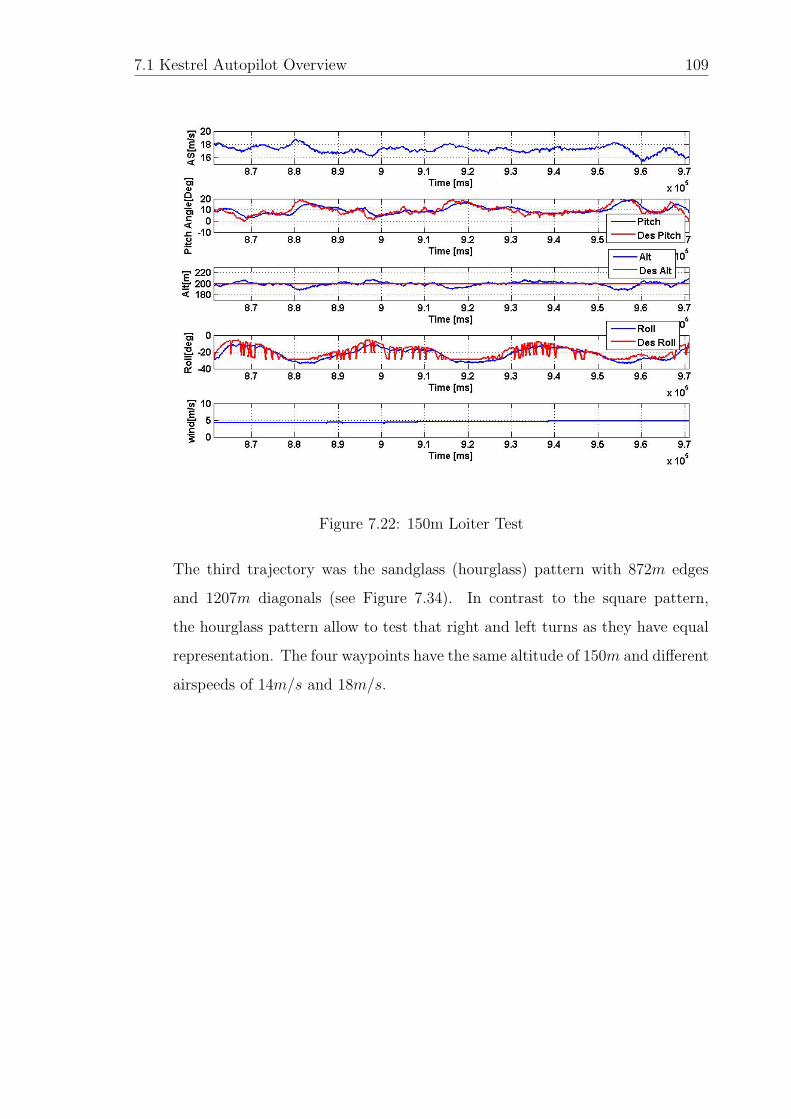
7.1 Kestrel Autopilot Overview 109
Figure 7.22: 150m Loiter Test
The third trajectory was the sandglass (hourglass) pattern with 872m edges
and 1207m diagonals (see Figure 7.34). In contrast to the square pattern,
the hourglass pattern allow to test that right and left turns as they have equal
representation. The four waypoints have the same altitude of 150m and different
airspeeds of 14m/s and 18m/s.

7.1 Kestrel Autopilot Overview 110
Figure 7.23: Error Analysis for the Altitude from the 150m Loiter Test
Figure 7.24: Error Analysis for the Pitch from the 150m Loiter Test
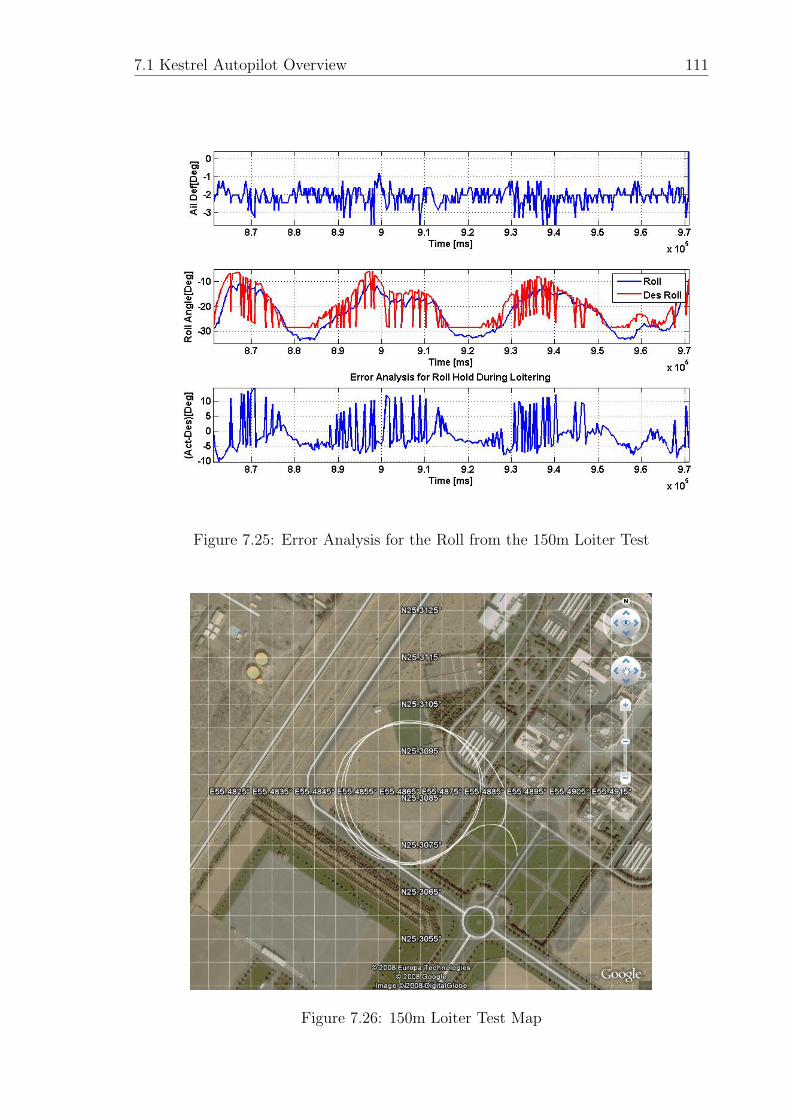
7.1 Kestrel Autopilot Overview 111
Figure 7.25: Error Analysis for the Roll from the 150m Loiter Test
Figure 7.26: 150m Loiter Test Map
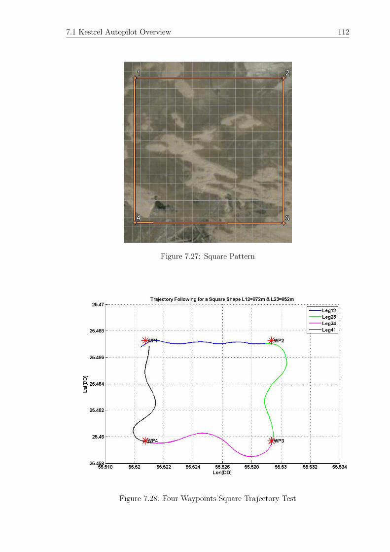
7.1 Kestrel Autopilot Overview 112
Figure 7.27: Square Pattern
Figure 7.28: Four Waypoints Square Trajectory Test
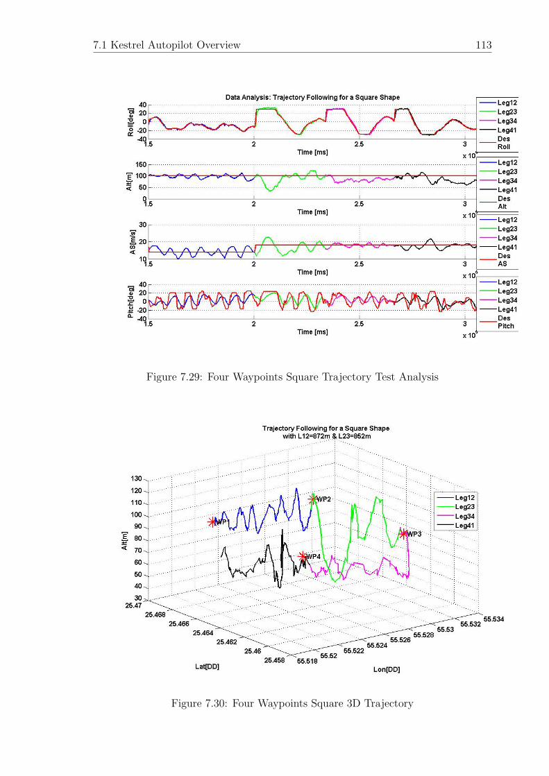
7.1 Kestrel Autopilot Overview 113
Figure 7.29: Four Waypoints Square Trajectory Test Analysis
Figure 7.30: Four Waypoints Square 3D Trajectory

7.1 Kestrel Autopilot Overview 114
Figure 7.31: Four Laps:Four Waypoints Square 2D Trajectory
Figure 7.32: Four Laps:Four Waypoints Square 3D Trajectory

7.1 Kestrel Autopilot Overview 115
Figure 7.33: Four Laps:Four Waypoints Square 3D Trajectory Map
Figure 7.34: Hourglass Pattern

7.1 Kestrel Autopilot Overview 116
Figure 7.35: Four Waypoints Hourglass Trajectory Test
Figure 7.36: Four Waypoints Hourglass Trajectory Test Analysis
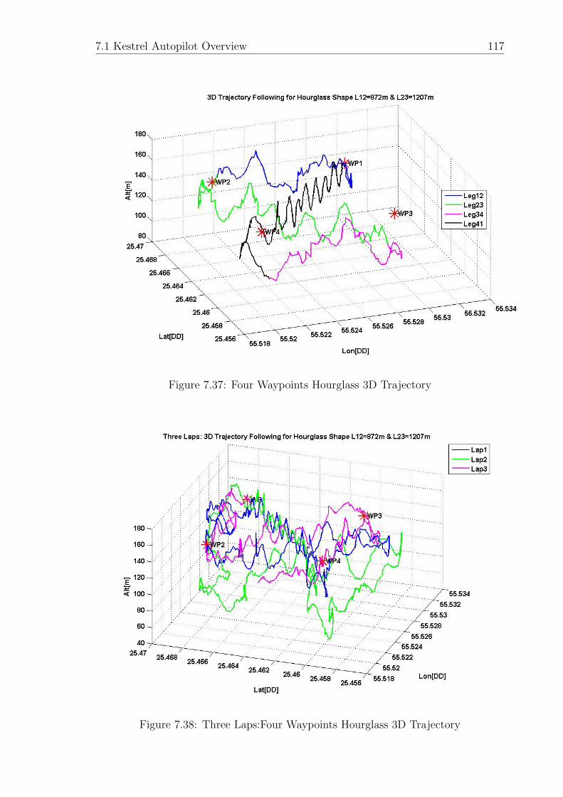
7.1 Kestrel Autopilot Overview 117
Figure 7.37: Four Waypoints Hourglass 3D Trajectory
Figure 7.38: Three Laps:Four Waypoints Hourglass 3D Trajectory
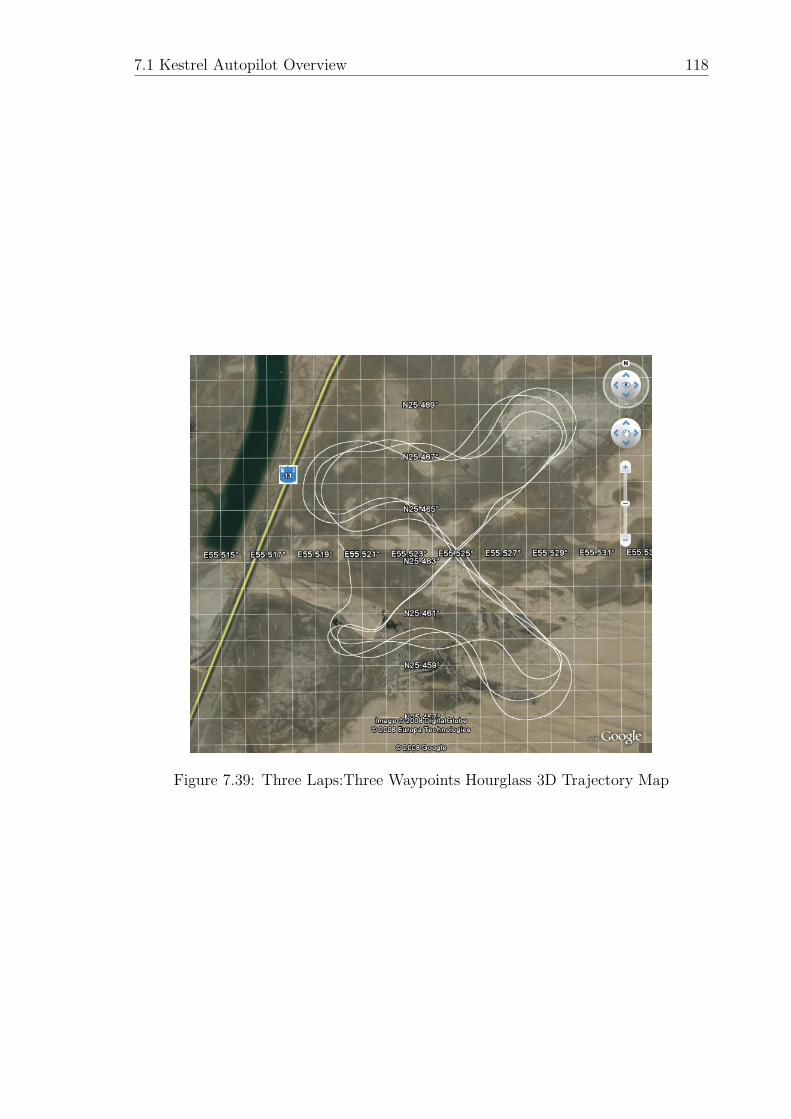
7.1 Kestrel Autopilot Overview 118
Figure 7.39: Three Laps:Three Waypoints Hourglass 3D Trajectory Map
Chapter 8
Thesis Summary and Future Work
In this chapter, the accomplished contributions in this thesis are summarized. Then,
recommendations for future research and development as follow-on to the work re-
ported in this thesis are provided
8.1 Summary and Contributions
8.1.1 Avionics Unit Development
A low cost avionics unit using commercial off the shelf components was designed, built
and tested. The designed avionics unit consists of a variety of sensors that consists of
basic electronics components. The total cost of the developed unit was around 9,000
US$.
8.1.2 System Identification and Aircraft Nonlinear Modelling
To be able to control the aircraft, a non-linear model is built. The aircraft stability
coefficients were estimated based on the aircraft geometry. To feed the controller with
the right aircraft states, both the engine and servo motors subsystems are identified
based on system identification techniques. Then, avionics unit sensors are modelled.
8.1.3 Developing Hardware in The Loop Simulation
To test the developed avionics unit performance, a Hardware In the Loop Simulation
was designed and tested on the aircraft non-linear model.
8.1.4 Implementing SLC Based Autopilot and Trajectory Tracking Using Simulink
Embedded Model-based Design
Improvements from previous versions of our work in AUS is the extensive use of
the interactive design using MATLAB/SIMULINK environment. Simulink Response

8.2 Future Work 120
Optimization, Control System Toolbox and Simulink Control Design are the major
tools used for the autopilot design to interact with Simulink. And the Target for
Freescale MPC5xx was used for the embedded system evaluation, implementation
and code generation of the design in real-time.
8.1.5 Developing Common Ground Station for UxV’s in AUS
A common and new ground station design was built and developed. The ground
station is developed using Visual Basic 2008 based software. The designed interface
consists of gauges to monitor speed, altitude, and aircraft attitudes. It also includes
a map that shows the position of the aircraft in the nearby area. Finally the GUI is
also used to upload commands directly to the aircraft.
8.1.6 Flight Testing
In this thesis, flight tests were conducted using Krestal autopilot to experiment with
flight testing and compare the performance with our avionics unit HILS results.
8.2 Future Work
8.2.1 Ground Station Enhancement
Ground station still can be enhanced as the project is improving and seeking for more
functions to be added to facilitate the user needs.
8.2.2 Nonlinear Autopilot and Trajectory Tracking Enhancement
In this thesis, a classical autopilot was designed for one trim condition. Future work
can put more in this area by going through the gain scheduling for different trim
conditions as well as designing a nonlinear autopilots. Moreover, with this designed
test bed, the research in the area of guidance and trajectory tracking can be given a
boost for algorithms validation.
8.2.3 Nonlinear System Identification
To get a better aircraft model, a nonlinear identification algorithms can be used and
developed.

Appendix A
Geometry, Aerodynamic, and other Aircraft
Design information
A.1 Aircraft Geometry Definitions
A.1.1 Wingspan
Wingspan of aircraft The wingspan of an aircraft is always measured in a straight
line, from wingtip to wingtip, independently of wing shape or sweep.
• Implications for aircraft design
Planes with a longer wingspan are generally more efficient because they suffer less
induced drag and their wingtip vortices do not affect the wing as much. However,
the long wings mean that the plane has a greater moment of inertia about its lon-
gitudinal axis and therefore cannot roll as quickly and is less maneuverable. Thus,
combat aircraft and aerobatic planes usually opt for shorter wingspans to increase
maneuverability.
Since the amount of lift that a wing generates is proportional to the area of the
wing, planes with short wings must correspondingly have a longer chord. An aircraft’s
ratio of its wingspan to chord is therefore very important in determining its charac-
teristics, and aerospace engineers call this value the aspect ratio of a wing.(Wikipedia
the free encyclopedia, )
A.1.2 Mean Aerodynamic Chord (MAC)
Finding the Mean Aerodynamic Chord (MAC) Many plans indicate that the Center of
Gravity (CG) should be located at a certain point of the Mean Aerodynamic Chord.
The CG can be measured from any point along the span from the leading edge of the
wing if the wing is a constant chord planform.

A.1 Aircraft Geometry Definitions 122
If the wing is tapered then you must locate the MAC before you can locate
the CG.
A.1.3 Aspect ratio (AR)
In aerodynamics, the aspect ratio is defined as span squared divided by wing area:
AR =b2
S
Informally, a high aspect ratio indicates long, narrow wings, whereas a low
aspect ratio indicates short, stubby wings.
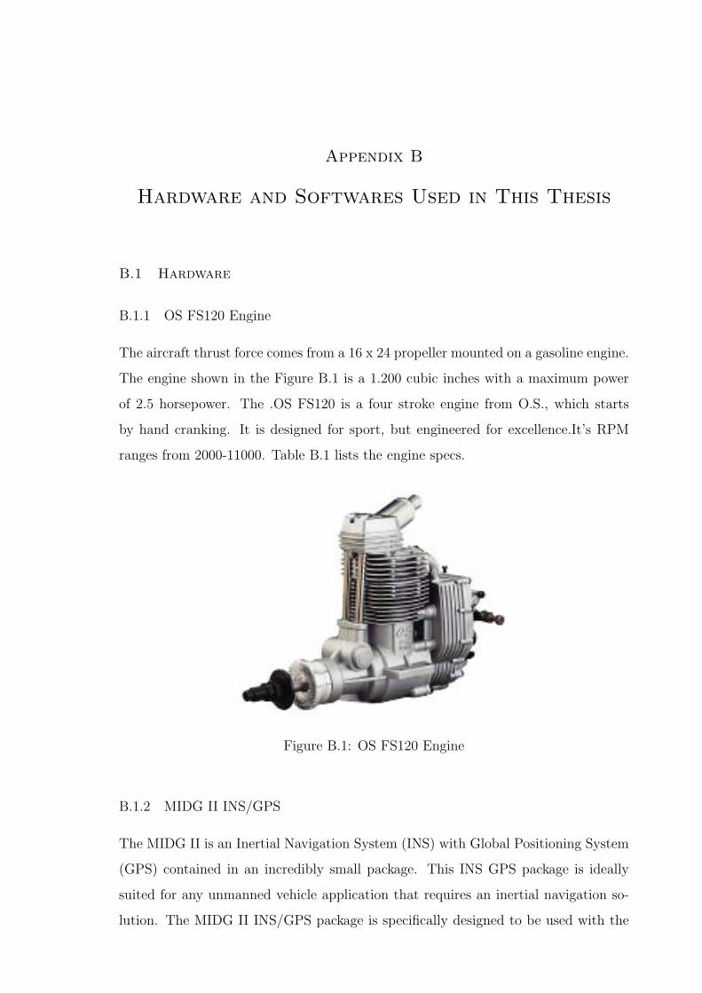
Appendix B
Hardware and Softwares Used in This Thesis
B.1 Hardware
B.1.1 OS FS120 Engine
The aircraft thrust force comes from a 16 x 24 propeller mounted on a gasoline engine.
The engine shown in the Figure B.1 is a 1.200 cubic inches with a maximum power
of 2.5 horsepower. The .OS FS120 is a four stroke engine from O.S., which starts
by hand cranking. It is designed for sport, but engineered for excellence.It’s RPM
ranges from 2000-11000. Table B.1 lists the engine specs.
Figure B.1: OS FS120 Engine
B.1.2 MIDG II INS/GPS
The MIDG II is an Inertial Navigation System (INS) with Global Positioning System
(GPS) contained in an incredibly small package. This INS GPS package is ideally
suited for any unmanned vehicle application that requires an inertial navigation so-
lution. The MIDG II INS/GPS package is specifically designed to be used with the

B.1 Hardware 124
Table B.1: S FS120 Engine Specifications
Engine Type 4-StrokeDisplacement 1.200 cu. in.
Cylinders 1Displacement 1.200 cubic inches
Bore 1.197 (in.)Stroke In 1.083 (in.)
Shaft 5/16 x 24 ThreadLow RPM 2000High RPM 11000
Horse Power 2.500 bhp @ 10000 RPMWeight (no muffler) 36.30 oz.
Figure B.2: MIDG II:Inertial Navigation System (INS) with Global Positioning Sys-tem (GPS)
Microbot Autopilot Platform, but can also be used with other autopilot packages for
primary instrumentation.
Message rates are configurable, and individual messages may be polled. All
data messages are time stamped with GPS time, and a One Pulse Per Second sig-
nal is available for time synchronization in the host computer. Operational mode
is selectable, including IMU only operation, vertical gyro simulation with magnetic
aiding, and full INS solution. MIDG is intended for use in applications requiring a full
state vector, including attitude, position, altitude, velocity, acceleration, and angular
rates.
MIDG II INS/GPS Product Features:
• Size : 1.50 x 1.58 x 0.88
• Weight : Under 55 grams (1.9 oz.)
• 3-Axis Rate Gyro

B.1 Hardware 125
Figure B.3: MMPX4115A Absolute Pressure Sensor
• 3-Axis Accelerometer
• 3-Axis Magnetometer
• Differential Ready GPS; WAAS/EGNOS compliant
• Power In: 10 to 32 VDC, 1.2W maximum
• Hardware filters provide vibration immunity
• Advanced filter algorithms for exceptional performance
• Position, Velocity, and Attitude from Kalman Filter at 50Hz
B.1.3 MPX4115A Absolute Pressure Sensor
The sensor we used in order to sense the absolute pressure is the Motorola MPX4115
shown in Figure ??. The Manifold Absolute Pressure (MAP) sensor is one of the
state of the art from its kinds, it costs around 30$.
Motorola MPX4115 is a piezoresistive transducer; which integrates on chip
bipolar op-amp circuitry and a thin film resistor network to provide a high output
signal and temperature compensation.
part comes with six pins of which only there are used. Pins 4, 5 and 6 are no
connections. Pin 1 is the output that varies with the air pressure while pins 2 and 3
are the VCC and the ground connections.
The sensor outputs an analog voltage proportional to pressure using a linear
equation. The sensor also as we mentioned before has on-chip signal conditioning to
produce an output range of 0.2V at (15Kpa) to 4.8V at (115Kpa).
B.1 Hardware 126
B.1.4 1INCHGBASIC Differential Pressure Sensor
The pitot tube is connected to a gauge pressure sensor to get a measurement of the
difference between the static and total pressures. We are using the 1INCHGBASIC
low pressure differential/gauge sensor fully signal conditioned.
Wind Tunnel experiments are used in meteorology and engineering sciences
to investigate flow over and around obstacles, such as mountains, airplane wings, or
vehicles, under controlled conditions. This experiment is designed to examine the
relationships between wind speed and the pressure it exerts, the effect of high winds
on vehicles, and the mechanism by which very high winds can destroy buildings.
In order to calibrate our gauge pressure sensor a wind tunnel test is used to
establish the wind-pressure relationships when air flows over a flat surface. The ”pitot
tube” sensor and a turbine anemometer are used to obtain both pressure and wind
speed.
Appendix C
Engine and Actuators System Identification
C.1 Engine System ID
To build the aircraft nonlinear model we need to characterize the engine response
to throttle command. The engine dynamics is a function of several inputs like fuel
inlet, manifold pressure, temperature, and air pressure. For simplicity we assume
that the other inputs are constant and we are only changing the throttle command.
An experiment has been conducted to get a transfer function that relates the throttle
command input to engine RPM and propeller thrust force output. The experiment
was applied on two engine-propeller assembly sets.
C.1.1 The Engine and its Propeller Modeling
The ARF60 AUS-UAV thrust is provided by fixed pitch propeller-internal combustion
engine assembly. Since one of the important roles for the propulsion system is to
provide enough thrust to balance the UAV drag during flight, a faithful mathemat-
ical model for the engine-propeller can be obtained to be used for constructing the
nonlinear mathematical model of the UAV.
Experimental Design
The data collected from the experimental setup are the engine thrust and the engine
RPM. The thrust is measured using load cell while the RPM is measured using IR
Reflective object sensor. The input signal is the duty cycle that controls the throttle
and is represented by the pseudo random binary sequence to excite all the dynamics
in the system. An introduction to the sensors utilized in this experiment, as well as
the experiment setup is provided.

C.2 Actuator System ID 128
RPM Sensor A sensor was needed to measure the engine RPM. The reading from
WW-01 WheelWatcher low cost incremental encoder system is utilized to mea-
sure the RPM. Both standard ChA/ChB raw quadrature outputs, as well as
decoded Clock and Direction signals are available. The clock signal produces
25µs pulses at each transition of ChA or ChB, providing a 4x increase in reso-
lution - 128 clocks per servo rotation - while the direction signal indicates the
decoded direction of rotation. The readings from each channel is recorded and
saved.
Load Cell Sensor A load cell is used to measure the thrust force that occurs on the
aircraft due to the rotation of the propeller. The load cell used is the Entran
ELPM series 1250N. The load cell was mounted on a frame that was used for the
experiment. Before using the load cell, it needs to be calibrated with a known
mass. The voltage output for a given weight is shown in table C.1. Equation
C.1 relates the load force to the output voltage according to the linear fitting
shown in Figure C.1.
Load[N ] = 0.52016× V oltage− 8.269 (C.1)
Experiment Setup Using dSPACE, an experiment has been made that takes a
throttle command as a pseudo random variable input. Then, the throttle com-
mand is fed to the throttle servo motor. The Engine RPM changes due to the
change in the fuel combustion rate. The encoder reads this RPM and sends its
data to dSPACE. Also due to the rotation of the engine the propeller will apply
a thrust force on the aircraft. This force is measured by the load cell and its
output is also saved in dSPACE. The experiment setup block diagram is shown
in C.2. Simulink-dSpace program used to generate the PRBS signal, RPM mea-
surement and thrust measurement. These results are shown in Figures C.3 ,
C.4 and C.5 respectively.
C.2 Actuator System ID
The control surfaces of the UAV are actuated by four identical R/C servo motors.
Each servo arm is coupled to the corresponding control surface via mechanical links.
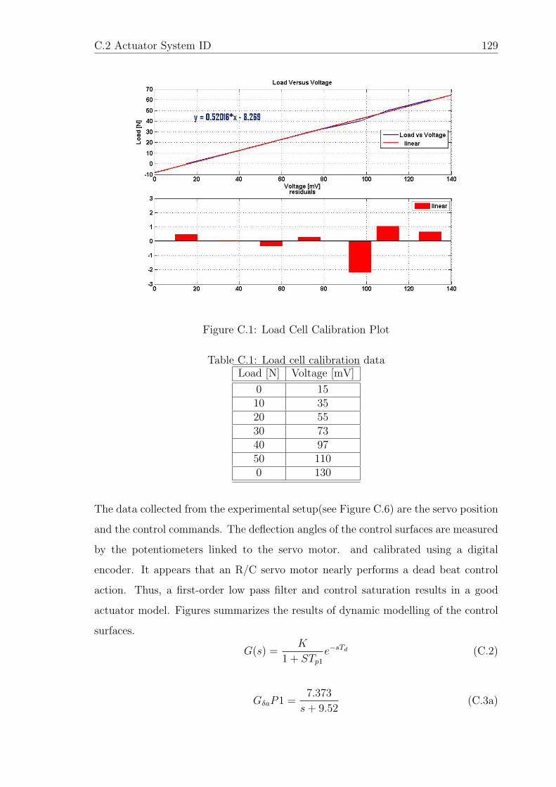
C.2 Actuator System ID 129
Figure C.1: Load Cell Calibration Plot
Table C.1: Load cell calibration dataLoad [N] Voltage [mV]
0 1510 3520 5530 7340 9750 1100 130
The data collected from the experimental setup(see Figure C.6) are the servo position
and the control commands. The deflection angles of the control surfaces are measured
by the potentiometers linked to the servo motor. and calibrated using a digital
encoder. It appears that an R/C servo motor nearly performs a dead beat control
action. Thus, a first-order low pass filter and control saturation results in a good
actuator model. Figures summarizes the results of dynamic modelling of the control
surfaces.
G(s) =K
1 + STp1
e−sTd (C.2)
GδaP1 =7.373
s+ 9.52(C.3a)
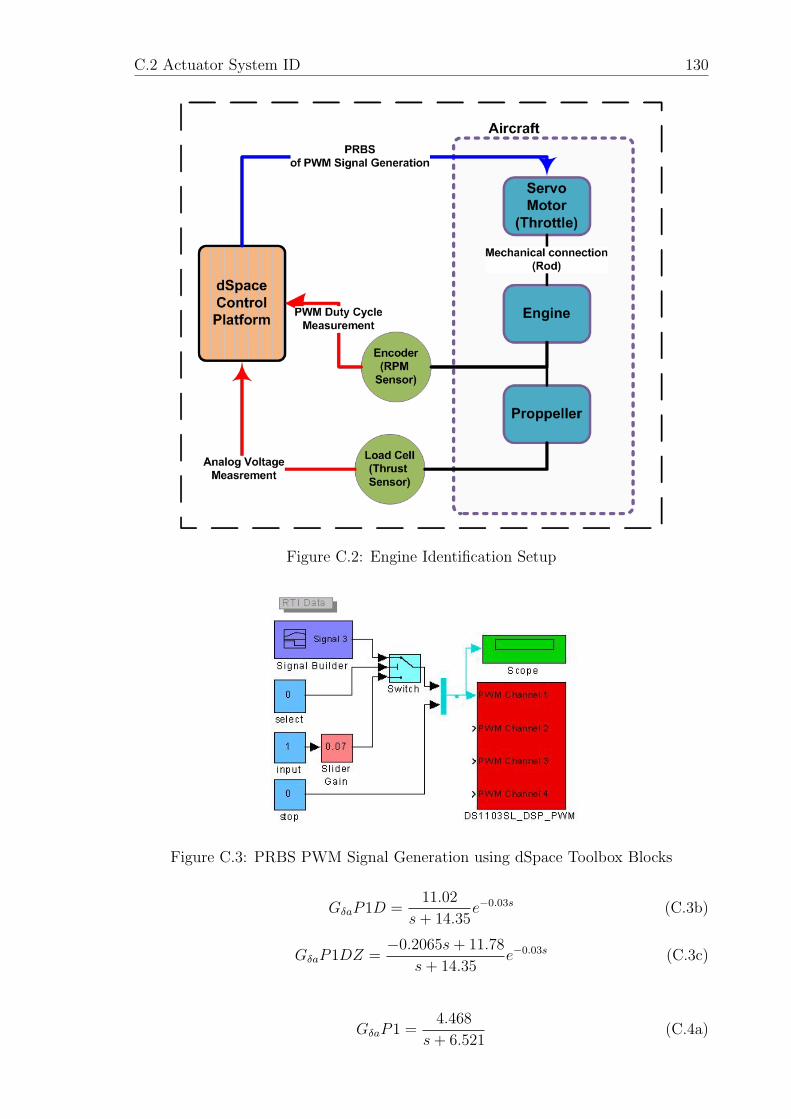
C.2 Actuator System ID 130
Figure C.2: Engine Identification Setup
Figure C.3: PRBS PWM Signal Generation using dSpace Toolbox Blocks
GδaP1D =11.02
s+ 14.35e−0.03s (C.3b)
GδaP1DZ =−0.2065s+ 11.78
s+ 14.35e−0.03s (C.3c)
GδaP1 =4.468
s+ 6.521(C.4a)

C.2 Actuator System ID 131
Figure C.4: RPM Measurement using dSpace Toolbox Blocks
Figure C.5: Thrust Measurement using dSpace Toolbox Blocks
GδaP1D =6.143
s+ 9.281e−0.03s (C.4b)
GδaP1DZ =−0.1826s+ 6.675
s+ 10.18e−0.03s (C.4c)
Figure C.6: Actuator Identifcation Setup

C.2 Actuator System ID 132
Figure C.7: Aileron actuator response with the doblets input
Figure C.8: Aileron Actuator Identifcation Results for Doublets inputs
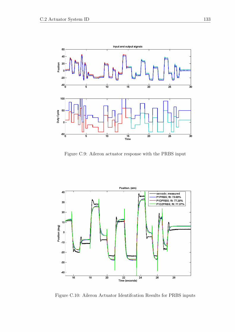
C.2 Actuator System ID 133
Figure C.9: Aileron actuator response with the PRBS input
Figure C.10: Aileron Actuator Identifcation Results for PRBS inputs
References
Beard, R. (2006). Vector field path following for small unmanned air vehicles. Pro-ceedings of the 2006 American Control Conference.
Bernard Etkin, L. D. R. (1996). Dynamics of Flight: Stabilty and Control. JohnWiley & Sons.
Bhatt S. P., K. P. (2005). A feedback guidance strategy for an autonomous mini-airvehicle. National Conference on Control and Dynamical Systems.
Chunhua Hu, Xingli Huang, J. H. & Zhu, J. (2004). System identification of asmall uavs speeding up process before take-off. The Proceedings of the 5th AsianControl Conference.
Dongwon Jung & Panagiotis Tsiotras (2007). Modeling and Hardware-in-the-LoopSimulation for a Small Unmanned Aerial Vehicle. American Institute of Aero-nautics and Astronautics, file = F.
dSPACE. dSPACE - Control Design.
Hadi, M. (Spring 2005). Autopilot design based on fuzzy supervisory controller foraus-autonomous vehicle. Master’s thesis, American University Sharjah (AUS).
Hassan, M. (Spring 2006). Aus-uav hils setup of dynamic flight path planning. Mas-ter’s thesis, American University Sharjah (AUS).
Holland, G. (1998). http://www.aerosonde.com/drawarticle/42.
Jung, S. (2001). Autopilot design for the stanford dragonfly uav: Validation throughhardware-in-the-loop simulation. AIAA.
Kaminer, A. Pascoal, E. H. & Silvestre, C. (1998). Trajectory tracking for autonomousvehicles: An integrated approach to guidance and control. AIAA Guidance,Control Dynamics, 21 (1), 29–38.
Leonardo, D. RS232 Blockset for Simulink.
Li-Xin Wang (1995). Design and analysis of fuzzy identifiers of nonlinear dynamicsystems. IEEE transactions on automatic control.
Peddle, I. K. (2005). Autonomous flight of a model aircraft. Master’s thesis, Universityof Stellenbosch.
Pike, J. (2005). http://www.globalsecurity.org/military/systems/aircraft/x-47.htm.
R. Connor, R. E. L. (2001). http://www.nasm.si.edu/research/aero/aircraft/pioneer.htm.

R. Pintelon & J. Schoukens. (2001). System Identification: A Frequency DomainApproach (1st ed.). Wiley-IEEE Press.
Randal W. Beard, T. W. M. (2007). An Introduction to Autonomous Miniature AirVehicles. Brigham Young University.
Rauw, M. . (1992). Using SIMULINK for Nonlinear Analysis of Aircraft ControlSystems. PhD thesis, Delft University of Technology (Aerospace Engineering).
Rolf, R. (September 2003). Uav path following for constant line of sight. AIAA Un-manned Unlimited Systems, Technologies and Operations Conference,San Diego,CA.
S. Park, J. D. & How, J. (Aug. 2004). A new nonlinear guidance logic for trajectorytracking. AIAA Guidance, Navigation Control Conference.
Shaaban, A. (2006). Real-time Validation and Comparison of Fuzzy Identificationand State-space Identification for a UAV Platform.
v1.9.1, F. (2009). FlightGear Flight Simulator.
Vladislav Klein & Eugene A. Morell (2006). Aircraft System Identification: Theoryand Practice (1st Edition ed.). American Institute of Aeronautics and Astroanu-tics,AIAA.
Wikipedia the free encyclopedia. www.wikipedia.org.
Wise, R. (2006). UAV Control and Guidance for Autonomous Cooperative Trackingof a Moving Target. PhD thesis, University of Washington.
Zadeh, L. (2007). The Fuzzification of Systems, volume Volume 216/2007, chapterFrom Circuit Theory to System Theory, (pp. 165–200). Springer Berlin / Hei-delberg.