GUIDE FOR PAVEMENT FRICTION

i

1 2

TABLE OF CONTENTS 3 4 5 LIST OF FIGURES.......................................................................... ii 6 7 LIST OF TABLES ........................................................................... iii 8 9 ACKNOWLEDGMENTS ................................................................ iv 10 11 ABSTRACT ........................................................................................v 12 13 1. INTRODUCTION.........................................................................1 14 1.1 BACKGROUND ........................................................................................... 1 15 1.2 PURPOSE AND SCOPE OF GUIDE.............................................................. 1 16 1.3 GUIDE ORGANIZATION AND USE.............................................................. 2 17 18 2. PAVEMENT FRICTION OVERVIEW .....................................3 19 2.1 IMPORTANCE OF PAVEMENT FRICTION ................................................... 3 20 2.2 PAVEMENT FRICTION PRINCIPLES.......................................................... 6 21 22 3. PAVEMENT FRICTION MANAGEMENT............................21 23 3.1 DEVELOPING PAVEMENT FRICTION MANAGEMENT POLICIES............. 22 24 3.2 ESTABLISHING THE PAVEMENT FRICTION MANAGEMENT PROGRAM.. 24 25 26 4. PAVEMENT FRICTION DESIGN..........................................39 27 4.1 INTRODUCTION ....................................................................................... 39 28 4.2 DEVELOPING FRICTION DESIGN POLICIES ........................................... 39 29 4.3 PROJECT-LEVEL DESIGN GUIDELINES ................................................. 52 30 31 REFERENCES ................................................................................60 32 33 APPENDIX A. TERMINOLOGY 34 35 APPENDIX B. STANDARDS RELEVANT TO PAVEMENT 36 FRICTION 37 38 39

ii

LIST OF FIGURES 1 2 Page 3 Figure 1. Total crashes (from all vehicle types) on U.S. highways from 1990 4 to 2003 (NHTSA, 2004)........................................................................................ 3 5 Figure 2. Total fatalities (from all vehicle types) on U.S. highways from 1990 6 to 2003 (NHTSA, 2004)........................................................................................ 4 7 Figure 3. Relationship between wet-weather crash rates and pavement friction 8 (Rizenbergs et al., 1973) ...................................................................................... 5 9 Figure 4. Mean crash risk for roadway network in the United Kingdom 10 (Viner et al., 2004) ............................................................................................... 5 11 Figure 5. Simplified diagram of forces acting on a rotating wheel ................................... 6 12 Figure 6. Pavement longitudinal friction versus tire slip (Henry, 2000).......................... 7 13 Figure 7. Dynamics of a vehicle traveling around a constant radius curve 14 at a constant speed, and the forces acting on the rotating wheel ..................... 8 15 Figure 8. Key mechanisms of pavement–tire friction ........................................................ 9 16 Figure 9. Simplified illustration of the various texture ranges that exist for a given 17 pavement surface (Sandburg, 1998) ................................................................. 11 18 Figure 10. Texture wavelength influence on pavement–tire interactions 19 (adapted from Henry, 2000 and Sandburg and Ejsmont, 2002)...................... 12 20 Figure 11. The IFI and Rado IFI models (Rado, 1994) ...................................................... 18 21 Figure 12. Example PFM program ..................................................................................... 23 22 Figure 13. Conceptual relationship between friction demand, speed, and friction 23 availability.......................................................................................................... 27 24 Figure 14. Setting of investigatory and intervention levels for a specific friction 25 demand category using time history of pavement friction .............................. 32 26 Figure 15. Setting of investigatory and intervention levels for a specific friction 27 demand category using time history of friction and crash rate history.......... 32 28 Figure 16. Setting of investigatory and intervention levels for a specific friction 29 demand category using pavement friction distribution and crash 30 rate–friction trend.............................................................................................. 33 31 Figure 17. Determination of friction and/or texture deficiencies using the IFI ............... 34 32 Figure 18. Example illustration of matching aggregate sources and mix types/ 33 texturing techniques to meet friction demand ................................................. 52 34 Figure 19. Example of determining DFT(20) and MPD needed to achieve design 35 friction level........................................................................................................ 55 36 Figure 20. Flowchart illustration of asphalt pavement friction design 37 methodology (Sullivan, 2005) ............................................................................ 56 38 Figure 21. Illustration of vehicle response as function of PSV and MTD 39 (Sullivan, 2005) .................................................................................................. 56 40 41 42 43 44

iii

LIST OF TABLES 1 2 Page 3 Table 1. Factors affecting available pavement friction 4 (Wallman and Astrom, 2001) ............................................................................ 10 5 Table 2. Summary of key issues to be considered in standardizing test conditions..... 29 6 Table 3. Assessment of hydroplaning potential based on vehicle speed and 7 water film thickness .......................................................................................... 36 8 Table 4. Test methods for characterizing aggregate frictional properties .................... 41 9 Table 5. Typical range of test values for aggregate properties...................................... 46 10 Table 6. Asphalt pavement surface mix types and texturing techniques ..................... 48 11 Table 7. Concrete pavement surface mix types and texturing techniques ................... 50 12 Table 8. Pairs of MPD and DFT(20) needed to achieve design friction level of 40....... 55 13 14 15 16

iv

ACKNOWLEDGMENTS 1 2 3 The research described herein was performed under NCHRP Project 1-43 by the 4 Transportation Sector of Applied Research Associates (ARA), Inc. Dr. Jim W. Hall, Jr., was 5 the Principal Investigator for the study. 6 7 Dr. Hall was supported in the research and in developing this Guide by ARA Research 8 Engineers Mr. Leslie Titus-Glover, Mr. Kelly Smith, and Mr. Lynn Evans, and by three 9 project consultants—Dr. James Wambold (President of CDRM, Inc. and Professor Emeritus 10 of Mechanical Engineering at Penn State University), Mr. Thomas Yager (Senior Research 11 Engineer at the NASA Langley Research Center), and Mr. Zoltan Rado (Senior Research 12 Associate at the Pennsylvania Transportation Institute). 13 14 The authors gratefully acknowledge all of the individuals with state departments of 15 transportation (DOTs) who responded to the pavement friction survey conducted for this 16 project. The authors also express their gratitude for the valuable input provided by 17 knowledgeable representatives of DOTs, paving associations, academia, and manufacturers 18 of friction measuring equipment, vehicle tires, and trucks. 19 20 21

v

ABSTRACT 1 2 3 This report contains guidelines and recommendations for managing and designing for 4 friction on highway pavements. The contents of this report will be of interest to highway 5 materials, construction, pavement management, safety, design, and research engineers, as 6 well as others concerned with the friction and related surface characteristics of highway 7 pavements. 8 9 Information is presented that emphasizes the importance of providing adequate levels of 10 friction for the safety of highway users. The factors that influence friction and the concepts 11 of how friction is determined (based on measurements of surface micro-texture and macro-12 texture) are discussed. Methods for monitoring the friction of in-service pavements and 13 determining appropriate actions in the case of friction deficiencies (friction management) 14 are described. Also, aggregate tests and criteria that help ensure adequate micro-texture 15 are presented, followed by a discussion of how paving mixtures and surface texturing 16 techniques can be selected so as to impart the macro-texture required to achieve the design 17 friction level. 18 19 20

This page intentionally left blank. 1 2 3 4

1

CHAPTER 1. INTRODUCTION 1 2 3 1.1 BACKGROUND 4 5 Pavement–tire friction (or, simply, pavement friction) is one of the primary factors 6 determining highway safety and, in particular, the probability of wet skidding crashes. 7 Highway agencies have recognized this fact since the 1920's (Moyer, 1959). The probability 8 of wet skidding crashes is reduced when friction between a vehicle tire and pavement is 9 high. 10 11 Skid-related crashes are determined by many factors, wet pavement friction being only one 12 of them. Other factors, such as road geometry, traffic characteristics, vehicle speed, and 13 weather conditions, must be considered together with friction data when evaluating the 14 safety of a particular section of roadway. 15 16 The Guide for Pavement Friction, Guidelines for Skid-Resistant Pavement Design, 17 published by the American Association of State Highway and Transportation Officials 18 (AASHTO) in 1976, recommended pavement specifications that would yield the desired 19 frictional properties upon completion of construction and that would maintain adequate 20 long-term friction. This Guide discussed the importance of aggregate selection and mixture 21 design for both asphalt- and concrete-surfaced pavements, and the role of micro-texture and 22 macro-texture in pavement surface friction. 23 24 Although much research has been conducted on pavement surface characteristics and 25 pavement–tire interactions since development of the 1976 Guide, the available information 26 is somewhat fragmented and has not been integrated into a comprehensive, systematic 27 approach for identifying friction needs and determining the optimum pavement strategy. 28 Exacerbating the problem are the changes that have taken place with time, including 29 changes in pavement construction materials and mixture design properties, construction 30 procedures and standards, vehicle and tire characteristics, traffic loading, and friction-31 testing methods and equipment. 32 33 Continued introduction of new materials and technologies, coupled with the increasing 34 focus on the needs of the highway user (safer and more comfortable roads), has placed even 35 greater demands on highway engineers to design and build longer lasting, cost-effective 36 pavements. This Guide for Pavement Friction should help highway engineers accomplish 37 such a task. 38 39 40 1.2 PURPOSE AND SCOPE OF GUIDE 41 42 This Guide for Pavement Friction was prepared under NCHRP Project 1-43 to provide 43 highway pavement practitioners with guidance in designing, constructing, and managing 44 pavement surfaces—as part of both new and rehabilitation projects—that meet the public’s 45 demand for safe friction levels, while recognizing and considering the effects of noise 46 generation and other pavement–tire interaction issues (e.g., splash and spray, tire wear). 47 48

2

The Guide contains recommendations and tools for upper-level administrators and policy-1 makers, as well as front-line pavement designers and managers. These recommendations 2 are intended to supplement but not replace an agency’s normal structural and/or mix 3 design practices. The Guide covers the following topics: 4 5

• Characteristics of pavement materials and surfaces that contribute to adequate wet-6 weather friction. 7

• Friction-testing methods, equipment, and indices. 8 • Methods for establishing friction levels that signify (a) design of new pavement 9

surfaces, (b) increased potential for skid-related crashes, and (c) the immediate need 10 for friction restoration. 11

• Guidance for aggregates, mixtures, and surface types that result in long-lasting, 12 high-quality friction surfaces, with proper consideration of noise, economics, and 13 other friction-related issues (e.g., splash and spray, hydroplaning, tire wear). 14

15 The Guide addresses both asphalt (i.e., flexible and semi-rigid) and concrete (i.e., rigid) 16 pavements associated with both original construction (i.e., new construction and 17 reconstruction) and maintenance and rehabilitation (M&R) treatments. It does not address 18 winter maintenance issues (i.e., snow and ice removal/treatment) and does not deal with 19 unpaved surfaces or non-highway pavements. 20 21 22 1.3 GUIDE ORGANIZATION AND USE 23 24 The Guide is divided into four chapters dealing with the importance of pavement friction, 25 the basic concepts of friction, how friction is measured and managed, and how to design for 26 friction. Following this introductory chapter, Chapter 2 discusses the importance of 27 providing adequate levels of friction for the safety of highway users and it provides an 28 overview of pavement friction (what it is, what influences it) and describes the equipment 29 and methods used to measure and report friction and texture. 30 31 Chapter 3 discusses friction from the management standpoint, covering both policy 32 development and the application of procedures for monitoring and restoring friction, based 33 on the principle of friction supply versus friction demand. Chapter 4 guides the user 34 through the surface friction design process. It discusses the development of design policies 35 that help promote long-term network-wide friction improvements, and provides project-36 level how-to guidance for designing pavements with proper friction. Lastly, a glossary of 37 terms is included in Appendix A to facilitate understanding of the terminology and 38 nomenclature contained in the Guide, and a list of standards relevant to pavement friction 39 is provided in Appendix B. 40

3

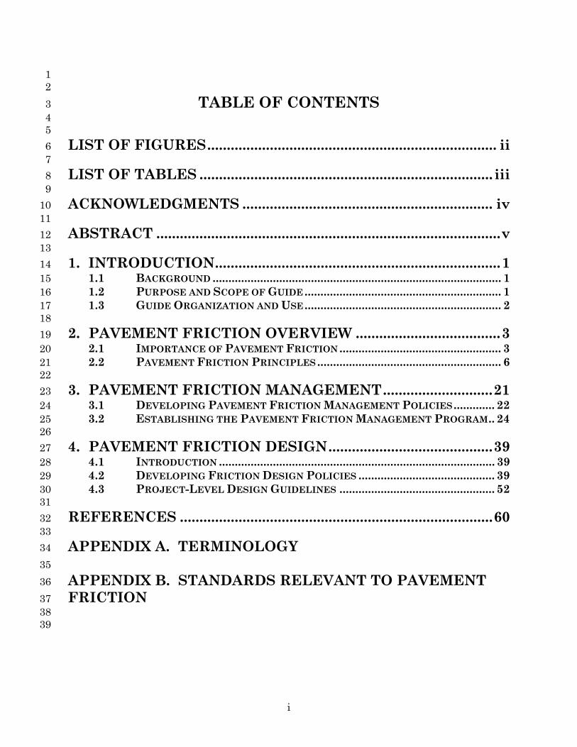
CHAPTER 2. PAVEMENT FRICTION OVERVIEW 1 2 3 2.1. IMPORTANCE OF PAVEMENT FRICTION 4 5 2.1.1 Highway Safety 6 7 Between 1990 and 2003, an average of 6.4 million highway crashes (all vehicle types) 8 occurred annually on the nation’s highways, resulting in 3 million injuries, 42,000 9 fatalities, and countless amounts of pain and suffering. This rate of fatality equates to 115 10 fatalities per day, or 1 death every 12 minutes (Noyce et al., 2005; National Highway 11 Traffic Safety Administration [NHTSA], 2004). In 2000, the cost of highway crashes was 12 estimated at $230.6 billion (Noyce et al., 2005; NHTSA, 2004). 13 14 Figures 1 and 2 present summaries of the total number of crashes and resulting fatalities 15 in the U.S. between 1990 and 2003. According to the National Transportation Safety Board 16 (NTSB) and the FHWA, approximately 13.5 percent of fatal crashes and 25 percent of all 17 crashes occur when roads are wet (Kuemmel et al., 2000). 18 19 One or more factors contribute to highway crashes. These factors fall under three main 20 categories: driver-related, vehicle-related, and highway condition-related (Noyce et al., 21 2005). Of these three categories, only highway condition can be controlled by highway 22 agencies through design, construction, maintenance, and management practices and 23 policies. Although many highway-related conditions influence safety (e.g., geometric 24 design, intersection and roadside design, pavement surface conditions [friction, texture, 25 distress, smoothness]), this Guide focuses on the provision and maintenance of adequate 26 levels of friction. 27 28 29 30 31 32 33 34 35 36 37 38 39 40 41 42 43 44 45 46

Figure 1. Total crashes (from all vehicles types) on U.S. highways from 1990 to 2003 47 (NHTSA, 2004). 48

5.6

5.8

6.0

6.2

6.4

6.6

6.8

7.0

1990

1991

1992

1993

1994

1995

1996

1997

1998

1999

2000

2001

2002

2003

Tota

l cra

shes

, mill

ions

5.6

5.8

6.0

6.2

6.4

6.6

6.8

7.0

1990

1991

1992

1993

1994

1995

1996

1997

1998

1999

2000

2001

2002

2003

Tota

l cra

shes

, mill

ions

4

1 2 3 4 5 6 7 8 9 10 11 12 13 14 15 16 17 18

Figure 2. Total fatalities (from all vehicles types) on U.S. highways from 19 1990 to 2003 (NHTSA, 2004). 20

21 22 2.1.2 Crash Reduction 23 24 The friction developed between vehicle tires and a pavement surface is a critical factor in 25 controlling and reducing crashes (Henry, 2000; Ivey et al., 1992). Studies conducted in the 26 U.S. and elsewhere have generally shown that wet-weather crash rates increase as 27 pavement friction decreases (all other factors such as speed and traffic volumes remaining 28 the same). For instance, as seen in figure 3, crash and measured pavement friction data 29 obtained from mostly rural interstates and parkway roads in Kentucky (Rizenbergs et al., 30 1973) showed increased wet crash rates at pavement friction values (SN40, skid/friction 31 number determined with a locked-wheel friction tester operated at 40 mi/hr [64 km/hr]) less 32 than 40 for low and moderate traffic levels. 33 34 In a study for the Texas Department of Transportation (TXDOT), McCullough et al. (1966) 35 found increasing fatal and injury crashes with decreasing coefficient of friction at 50 mi/hr 36 (80 km/hr). More recent research in this area (Agent et al., 1996; Wallman and Astrom, 37 2001) has provided similar trends, emphasizing the need to design for, monitor, and 38 expeditiously restore pavement surface friction properties. Recent research in the United 39 Kingdom also indicated an increase in crash risk as friction levels are reduced. Figure 4 40 provides the relationships determined in that study for tangent alignments in both wet and 41 dry conditions (Viner et al., 2004). 42 43 Although research has confirmed a basic relationship between pavement friction and wet 44 crash rates, it has not established an exact relationship nor identified any specific threshold 45 friction values below which wet crash rates increase substantially (Henry, 2000; Larson, 46 1999). This is because friction demand (i.e., the level of friction needed to prevent a vehicle 47 from slipping or sliding) varies with location and time due to changing site conditions, 48 49

36

37

38

39

40

41

42

43

44

45

46

1990

1991

1992

1993

1994

1995

1996

1997

1998

1999

2000

2001

2002

2003

Tota

l Fat

aliti

es, t

hous

ands

5

1 2 3 4 5 6 7 8 9 10 11 12 13 14 15 16 17 18

19 20 21 22 23 24

Figure 3. Relationship between wet-weather crash rates and pavement friction 25 (Rizenbergs et al., 1973). 26

27 28 29 30 31 32 33 34 35 36 37 38 39 40 41 42 43 44 45 Figure 4. Mean crash risk for roadway network in the United Kingdom (Viner et al., 2004) 46

(Note: dual carriageway = 4-lane divided highway, single carriageway = undivided highway, 47 non-event = segments with no junctions, crossings, or notable bends or gradients). 48

49

0.3 0.35 0.4 0.45 0.5 0.55 0.6 Skid Resistance, Sideways Force Coefficient (SFC)

20

15

10

5

0 Mea

n C

rash

Ris

k, %

(def

ined

as

tota

l num

ber

of c

rash

es p

er 1

00

mil

lion

veh

icle

km

dri

ven)

Motorway Dual Carriageway non-event Single Carriageway non-event

6

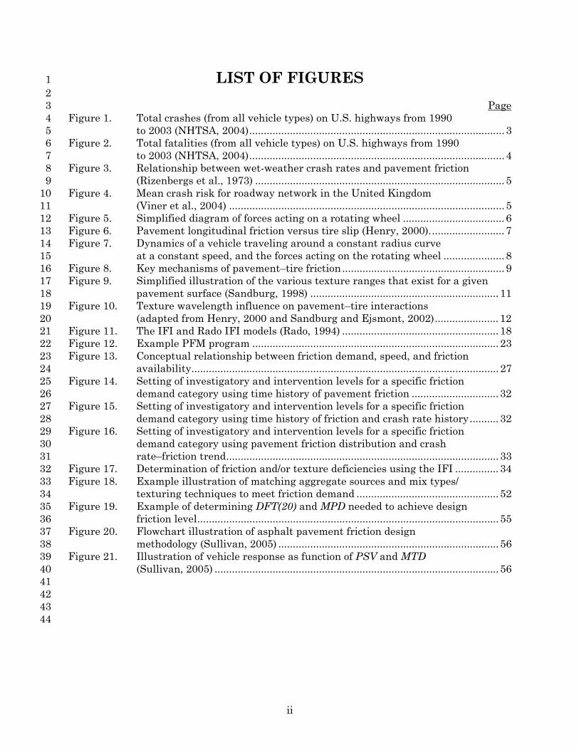
traffic characteristics, and driver/vehicle characteristics. While a particular friction value 1 may satisfy demand at one location and at one moment in time, the same value may not 2 satisfy the demand at another location or at a different moment in time. Thus, control of 3 friction at the network level must be based on periodic assessments of friction (and crashes) 4 at the pavement segment/unit level. 5 6 7 2.2 PAVEMENT FRICTION PRINCIPLES 8 9 2.2.1 Definition (of Pavement Friction) 10 11 Pavement friction is the force that resists the relative motion between a vehicle tire and a 12 pavement surface. This resistive force (illustrated in figure 5) is generated when the tire 13 rolls or slides over the pavement surface. A measure of the resistive force is the non-14 dimensional coefficient of friction, μ, which as expressed in equation 1, is the ratio of the 15 tangential friction force (F) between the tire tread rubber and the horizontal traveled 16 surface to the perpendicular force or vertical load (FW). 17 18 19 Eq. 1 20 21 22 23 24 25 26 27 28 29 30 31 32 33 34 35 36 37

Figure 5. Simplified diagram of forces acting on a rotating wheel. 38 39 40 Longitudinal Friction 41 42 For the longitudinal dynamic friction process between a rolling pneumatic tire and the road 43 surface, there are two modes of operation—free-rolling and constant-braked. In the free-44 rolling mode (no braking), the relative speed between the tire circumference and the 45 pavement—referred to as the slip speed—is zero. In the constant-braked mode, the slip 46 speed increases from zero to a potential maximum of the speed of the vehicle. The following 47 mathematical relationship explains slip speed (Meyer, 1982): 48

Weight, FW

Direction of motion

Rotation

Friction Force, F

FwF

=μ

7

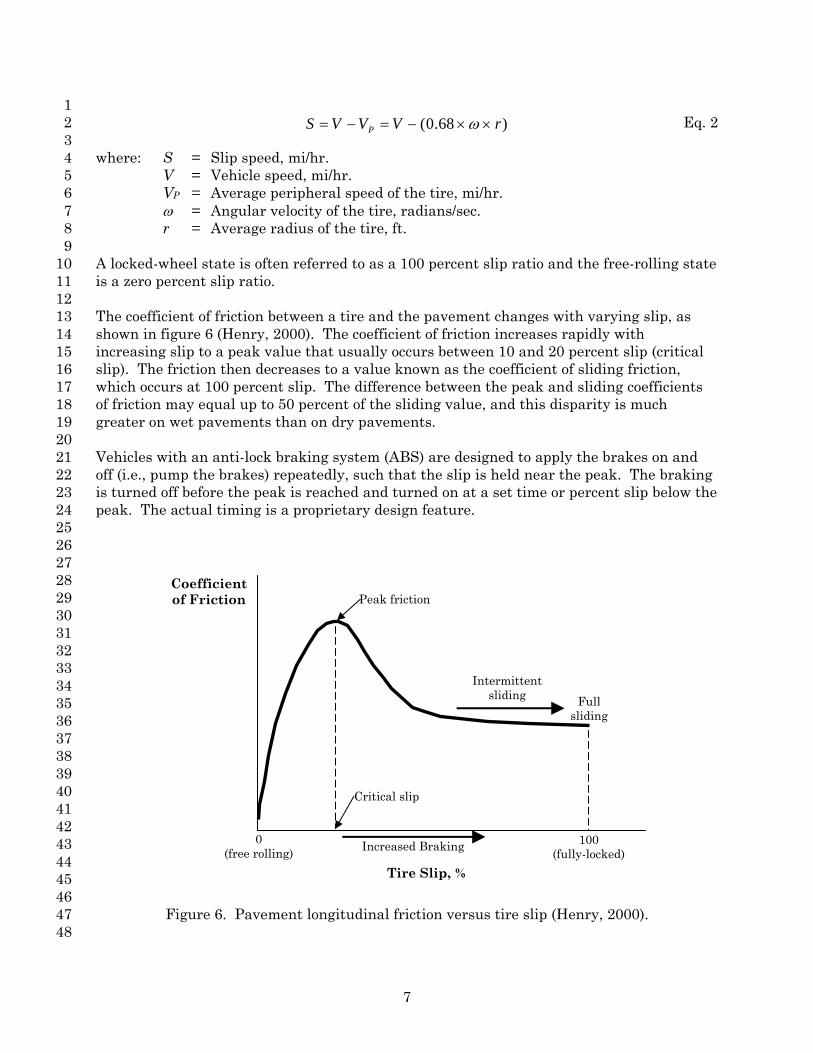
1 Eq. 2 2 3 where: S = Slip speed, mi/hr. 4 V = Vehicle speed, mi/hr. 5 VP = Average peripheral speed of the tire, mi/hr. 6 ω = Angular velocity of the tire, radians/sec. 7 r = Average radius of the tire, ft. 8 9 A locked-wheel state is often referred to as a 100 percent slip ratio and the free-rolling state 10 is a zero percent slip ratio. 11 12 The coefficient of friction between a tire and the pavement changes with varying slip, as 13 shown in figure 6 (Henry, 2000). The coefficient of friction increases rapidly with 14 increasing slip to a peak value that usually occurs between 10 and 20 percent slip (critical 15 slip). The friction then decreases to a value known as the coefficient of sliding friction, 16 which occurs at 100 percent slip. The difference between the peak and sliding coefficients 17 of friction may equal up to 50 percent of the sliding value, and this disparity is much 18 greater on wet pavements than on dry pavements. 19 20 Vehicles with an anti-lock braking system (ABS) are designed to apply the brakes on and 21 off (i.e., pump the brakes) repeatedly, such that the slip is held near the peak. The braking 22 is turned off before the peak is reached and turned on at a set time or percent slip below the 23 peak. The actual timing is a proprietary design feature. 24 25 26 27 28 29 30 31 32 33 34 35 36 37 38 39 40 41 42 43 44 45 46

Figure 6. Pavement longitudinal friction versus tire slip (Henry, 2000). 47 48

)68.0( rVVVS P ××−=−= ω

Peak friction

Critical slip

Full sliding

100 (fully-locked)

0 (free rolling)

Tire Slip, %

Coefficient of Friction

Increased Braking

Intermittent sliding

8

Side Force Friction 1 2 Another important aspect of friction relates to the lateral or side force friction that occurs 3 as a vehicle changes direction or compensates for pavement cross-slope and/or cross-wind 4 effects. The pavement–tire steering/cornering force diagram in figure 7 shows how the side 5 force friction factor acts as a counter balance to the centripetal force developed as a vehicle 6 performs a lateral movement. The basic relationship between the forces acting on the 7 vehicle tire and the pavement surface as the vehicle steers around a curve, changes lanes, 8 or compensates for lateral forces is as follows (AASHTO, 2001): 9 10 11 Eq. 3 12 13 14 where: FS = Side friction. 15 V = Vehicle speed, mi/hr. 16 R = Radius of the path of the vehicle’s center of gravity (also, the radius of 17 curvature in a curve), ft. 18 e = Pavement superelevation, ft/ft. 19 20 21 22 23 24 25 26 27 28 29 30 31 32 33 34 35 36 37 38 39 40 41 42 43

Figure 7. Dynamics of a vehicle traveling around a constant radius curve 44 at a constant speed, and the forces acting on the rotating wheel. 45

46 47

W Weight of vehicle P Centripetal force (horizontal) FS Friction force between tires and roadway surface (parallel to roadway surface) α Angle of super-elevation (tan α = e) R Radius of curve

α

α

W

P FS

Direction of Travel

Drag Force

Side Friction Force (Friction Factor)

Friction Measuring Wheel

eR

VFS −=15

2

9

Combined Braking and Cornering 1 2 With combined braking and cornering, a driver either risks not stopping as rapidly or losing 3 control due to reduced lateral/side forces. The interaction of the longitudinal and lateral 4 forces is such that as one force increases, the other must decrease by a proportional 5 amount. Commonly referred to as the friction circle or friction ellipse (Radt and Milliken, 6 1960), the vector sum of the two combined forces when depicted graphically (longitudinal 7 force on the x-axis and lateral force on the y-axis, or vice versa) remains constant (circle) or 8 near constant (ellipse). The degree of ellipse or circle depends on the tire and pavement 9 properties. 10 11 2.2.2 Mechanisms (of Pavement Friction) 12 13 Pavement friction is the result of a complex interplay between two principal frictional force 14 components—adhesion and hysteresis (figure 8). Although there are other components of 15 pavement friction (e.g., tire rubber shear), they are insignificant when compared to the 16 adhesion and hysteresis force components. Thus, friction can be viewed as the sum of the 17 adhesion and hysteresis frictional forces: 18 19 Eq. 4 20 21 22 23 24 25 26 27 28 29 30 31 32 33 34 35 36 37 38 39

40 Figure 8. Key mechanisms of pavement–tire friction. 41

42 43 Adhesion is the friction that results from the small-scale bonding/interlocking of the vehicle 44 tire rubber and the pavement surface as they come into contact with each other. It is a 45 function of the interface shear strength and contact area. The hysteresis component of 46 frictional forces results from the energy loss due to bulk deformation of the vehicle tire. 47 The deformation is commonly referred to as enveloping of the tire around the texture. 48 When a tire compresses against the pavement surface, the stress distribution causes the 49

Hysteresis Depends mostly on macro-level surface roughness

Adhesion Depends mostly on micro-level surface roughness

Rubber Element

V

F

HA FFF +=

10

deformation energy to be stored within the rubber. As the tire relaxes, part of the stored 1 energy is recovered, while the other part is lost in the form of heat (hysteresis), which is 2 irreversible. That loss leaves a net frictional force to help stop the forward motion. 3 4 Surface texture influences both mechanisms. The adhesion force is proportional to the real 5 area of adhesion between the tire and surface asperities. The hysteresis force is generated 6 within the deflecting and visco-elastic tire tread material, and is a function of speed. 7 Generally, adhesion is related to micro-texture, whereas hysteresis is mainly related to 8 macro-texture. For wet pavements, adhesion drops off with increased speed, while 9 hysteresis increases with speed. Also, because tire rubber is a visco-elastic material, each 10 component is affected by temperature and sliding speed. 11 12 2.2.3 Factors Affecting Available Pavement Friction 13 14 The factors that influence pavement friction forces can be grouped into four categories—15 pavement surface characteristics, vehicle operational parameters, tire properties, and 16 environmental factors. Table 1 lists the various factors comprising each category. Because 17 each factor in this table plays a role in defining pavement friction, friction must be viewed 18 as a process instead of an inherent property of the pavement. It is only when all these 19 factors are fully specified that friction takes on a definite value. 20 21 The more critical factors are shown in bold in table 1 and are briefly discussed below. 22 Among these factors, the ones considered to be within a highway agency’s control are micro- 23 and macro-texture, pavement material properties, and slip speed. 24 25 26

Table 1. Factors affecting available pavement friction (Wallman and Astrom, 2001). 27 28

Pavement Surface Characteristics

Vehicle Operating Parameters

Tire Properties

Environment

• Micro-texture • Macro-texture • Mega-texture/

unevenness • Material properties • Temperature

• Slip speed vehicle speed braking action

• Driving maneuver turning overtaking

• Foot Print • Tread design and

condition • Rubber composition

and hardness • Inflation pressure • Load • Temperature

• Climate Wind Temperature Water (rainfall, condensation) Snow and Ice

• Contaminants Anti-skid material (salt, sand) Dirt, mud, debris

Note: Critical factors are shown in bold. 29 30 31 Pavement Surface Texture 32 33 Pavement surface texture is made up of the deviations of the pavement surface from a true 34 planar surface. These deviations occur at three distinct levels of scale, each defined by the 35 wavelength (λ) and peak-to-peak amplitude (A) of its components. The three levels of 36 texture, as established by the Permanent International Association of Road Congresses 37 (PIARC) (1987), are as follows: 38 39

11

• Micro-texture (λ < 0.02 in [0.5 mm], A = 0.04 to 20 mils [1 to 500 µm])—Surface 1 roughness quality at the sub-visible/microscopic level. It is a function of the surface 2 properties of the aggregate particles within the asphalt or concrete paving material. 3

4 • Macro-texture (λ = 0.02 to 2 in [0.5 to 50 mm], A = 0.005 to 0.8 in [0.1 to 20 mm])—5

Surface roughness quality defined by the mixture properties (shape, size, and 6 gradation of aggregate) of an asphalt paving material and the method of 7 finishing/texturing (dragging, tining, grooving; depth, width, spacing and orientation 8 of channels/grooves) used on a concrete paving material. 9

10 • Mega-texture (λ = 2 to 20 in [50 to 500 mm], A = 0.005 to 2 in [0.1 to 50 mm])—This 11

type of texture is the texture which has wavelengths in the same order of size as the 12 pavement–tire interface. It is largely defined by the distress, defects, or “waviness” 13 on the pavement surface. 14

15 Wavelengths longer than the upper limit (20 in [500 mm]) of mega-texture are defined as 16 roughness or unevenness (Henry, 2000). Figure 9 illustrates the three texture ranges, as 17 well as a fourth level—roughness/unevenness—representing wavelengths longer than the 18 upper limit (20 in [500 mm]) of mega-texture (Sandburg, 1998). 19 20 It is widely recognized that pavement surface texture influences many different pavement–21 tire interactions. Figure 10 shows the ranges of texture wavelengths affecting various 22 vehicle–road interactions, including friction, interior and exterior noise, splash and spray, 23 rolling resistance, and tire wear. As can be seen, friction is affected primarily by micro-24 texture and macro-texture, which correspond to the adhesion and hysteresis friction 25 components, respectively. 26 27 28 29 30 31 32 33 34 35 36 37 38 39 40 41 42 43 44 45

Figure 9. Simplified illustration of the various texture ranges that exist for a given 46 pavement surface (Sandburg, 1998). 47

48

Roughness/Unevenness

Reference Length

Short stretch of road

Tire Mega-texture

Amplification ca. 50 times

Amplification ca. 5 times

Amplification ca. 5 times

Road–Tire Contact Area

Macro-texture

Micro-texture Single

Chipping

12

1 2 3 4 5 6 7 8 9 10 11 12 13 14 15 16 17 18 19

Figure 10. Texture wavelength influence on pavement–tire interactions 20 (adapted from Henry, 2000 and Sandburg and Ejsmont, 2002). 21

22 23 At low speeds, micro-texture dominates the wet and dry friction level. At higher speeds, 24 the presence of high macro-texture facilitates the drainage of water so that the adhesive 25 component of friction afforded by micro-texture is re-established by being above the water. 26 Hysteresis increases with speed exponentially, and at speeds above 65 mi/hr (105 km/hr) 27 accounts for over 95 percent of the friction (PIARC, 1987). 28 29 Pavement Surface Material Properties 30 31 Pavement material properties (i.e., aggregate and mix characteristics, surface texturings) 32 influence both micro-texture and macro-texture. These properties also affect the long-term 33 durability of texture through their capacities to resist aggregate polishing and abrasion/ 34 wear of both aggregate and mix under accumulated traffic and environmental loadings. 35 36 Slip Speed 37 38 The coefficient of friction between a tire and the pavement changes with varying slip. It 39 increases rapidly with increasing slip to a peak value that usually occurs between 10 and 40 20 percent slip. The friction then decreases to a value known as the coefficient of sliding 41 friction, which occurs at 100 percent slip. 42 43 Tire Tread Design and Condition 44 45 Tire tread design (i.e., type, pattern, and depth) and condition have a significant influence 46 on draining water that accumulates at the pavement surface. Water trapped between the 47 pavement and the tire can be expelled through the channels provided by the pavement 48 macro-texture and by the tire tread. Tread depth is particularly important for vehicles 49

10-6 10-5 10-4 10-3 10-2 10-1 100 101 Micro-texture Macro-texture Mega-texture Roughness/Unevenness

Int. Noise

Splash/Spray

Rolling Resistance

Tire/Vehicle

Texture Wavelength

Note: Darker shading indicates more favorable effect of texture over this range.

0.00001 0.0001 0.001 0.01 0.1 1 10 100 ft

Tire Wear

Ext. Noise

Friction

13

driving over thick films of water at high speeds. Some studies (Henry, 1983) have reported 1 a decrease in wet friction of 45 to 70 percent for fully worn tires as compared to new ones. 2 3 Tire Inflation Pressure 4 5 High inflation pressure causes only a small loss of pavement friction, whereas low inflation 6 pressure can significantly reduce friction at high speeds (Henry, 1983). This is because of 7 the constriction of drainage channels within the tire tread and reduced contact pressure. 8 9 Temperature 10 11 Friction of natural rubber tires has a large dependence on temperature, especially when 12 going through the freezing point. Modern rubber compounds are formulated to remove the 13 effect of temperature on friction. Since hysteresis is affected by the visco-elastic property of 14 the tire, friction is reduced at high temperatures where the rubber becomes soft. However, 15 these temperatures are above the normal running speeds and temperatures. When a lot of 16 braking is performed, these higher temperatures can be reached, however the brakes would 17 fade first. Perhaps the biggest effect is under locked-wheel conditions, where the rubber 18 can melt and cause rubber hydroplaning. 19 20 Surface Water 21 22 The effect of surface water layer depth (or water film thickness [WFT]) on friction is 23 minimal at low speeds (<20 mi/hr [32 km/hr]) and quite pronounced at higher speeds (>40 24 mi/hr [64 km/hr]). The coefficient of friction of a vehicle tire sliding over a wet pavement 25 surface, decreases exponentially as WFT increases. The effect of WFT is influenced by tire 26 design and condition, with worn tires being most sensitive to WFT. 27 28 A particularly hazardous situation involving relatively thick water films and vehicles 29 traveling at higher speeds is hydroplaning. Hydroplaning occurs when a vehicle tire is 30 separated from the pavement surface by the water pressure that builds up at the 31 pavement–tire interface (Horne and Buhlmann, 1983), causing friction to drop to near zero. 32 This phenomenon is affected by several parameters, including water depth, vehicle speed, 33 pavement macro-texture, tire inflation pressure and tread depth, and tire contact area. 34 35 Snow and Ice 36 37 Ice and snow covering the pavement surface present the most hazardous condition for 38 vehicle braking or cornering. The level of friction between the tires and the snow- or ice-39 covered pavement is such that almost any abrupt braking or sudden change of direction 40 results in locked-wheel sliding and loss of vehicle directional stability. This Guide does not 41 address winter-related friction issues. 42 43 2.2.4 Friction and Texture Measurement Methods 44 45 Overview 46 47 The measurement of pavement friction and texture has been of primary importance to state 48 highway agencies (SHAs) for at least 50 years. Many different types of equipment have 49

14

been developed and used to measure these properties. Their differences, in terms of 1 measurement principles and procedures and the way measurement data are processed and 2 reported, can be significant. 3 4 For friction-testing alone, there are several commercial devices that can operate at fixed or 5 variable slip, at speeds up to 100 mi/hr (161 km/hr), and under variable test tire conditions, 6 such as load, size, tread design and construction, and inflation pressure. Measurement of 7 pavement surface texture can be done using a variety of laser devices, volumetric 8 techniques, water drainage rates (outflow meter), and sliding rubber pad apparatus 9 (portable British Pendulum Tester [BPT]). This section provides an overview of the 10 different friction and texture measurement methods and available representative 11 equipment. 12 13 Methods and Equipment 14 15 AASHTO and ASTM have developed a set of surface characteristic standards and 16 measurement practice standards for both friction and texture. These standards ensure 17 comparability of the measurements for specific purposes; they are grouped according to 18 measurements performed at highway speeds (i.e., high-speed devices) and measurements 19 requiring lane closure (i.e., low-speed/walking and stationary devices). 20 21 In general, the measurement devices requiring lane closure are simpler and relatively 22 inexpensive, whereas the highway-speed devices are more expensive and require more 23 training to maintain and operate. With the recent development of technology in data 24 acquisition, sensor technology, and data processing power of computers, the once true 25 superiority of data quality for the stationary and low-speed devices is diminishing. The 26 resolution and accuracy of the acquired data for the measurement devices that are low-27 speed or stationary can be still superseding that of the high-speed devices, but with smaller 28 and smaller margins. 29 30 The locked-wheel friction tester (AASHTO T 242) is the predominant high-speed device 31 used on U.S. roads. This device requires a tow vehicle and a locked-wheel skid trailer, 32 equipped with either a standard ribbed tire(AASHTO M 261) or a standard smooth 33 tire(AASHTO M 286). Friction measurements are obtained by locking the test tire (ribbed 34 or smooth) on a wetted pavement surface while traveling at a specified speed (40 mi/hr [64 35 km/hr] is the standard speed given inAASHTO T 242). The smooth tire is more sensitive to 36 pavement macro-texture, while the ribbed tire is more sensitive to micro-texture changes in 37 the pavement. 38 39 Portable friction measurement equipment requiring lane closures include the 40 BPT(AASHTO T 278) and the Dynamic Friction Tester (DFT) (ASTM E 1911). 41 42

• The manually operated BPT provides an indicator of friction through the swinging of 43 a pendulum-based rubber slider and its contact with the pavement surface. The 44 elevation to which the pendulum swings after contact provides the basis for the 45 friction indicator, termed British Pendulum Number (BPN). 46

15

1 • The DFT is an electronic modular system that measures the torque necessary to 2

rotate three small, spring-loaded rubber pads in a circular path over a wetted 3 pavement surface at different speeds. Results are typically recorded at 12, 24, 36, 4 and 48 mi/hr (20, 40, 60, and 80 km/hr), from which the speed–friction relationship 5 is plotted. 6

7 High-speed texture measuring equipment includes laser profilers, such as the FHWA Road 8 Surface Analyzer (ROSANV). These non-contact devices use a combination of a horizontal 9 distance measuring device, a very high-speed (64 kHz or higher) laser triangulation sensor, 10 and a portable computer to collect and store pavement surface elevations (vertical 11 resolution usually 0.002 in [0.5 mm] or better) at intervals of 0.01 in (0.25 mm) or less. 12 From these elevations, the system calculates the mean profile depth (MPD), which is an 13 overall measure of macro-texture. 14 15 Texture measuring equipment requiring lane closures include the Sand Patch Method 16 (SPM) (ASTM E 965), the Outflow Meter (OFM) (ASTM E 2380), and the Circular Texture 17 Meter (CTM) (ASTM E 2157). 18 19

• The SPM is a volumetric-based spot test method that assesses pavement surface 20 macro-texture through the spreading of a known volume of glass beads in a circle 21 onto a cleaned surface and the measurement of the diameter of the resulting circle. 22 The volume divided by the area of the circle is reported as the mean texture depth 23 (MTD). 24

25 • The OFM is a volumetric test method that measures the water drainage rate 26

through surface texture and interior voids. It indicates the hydroplaning potential 27 of a surface by relating to the escape time of water beneath a moving tire. The 28 equipment consists of a cylinder with a rubber ring on the bottom and an open top. 29 Sensors measure the time required for a known volume of water to pass under the 30 seal or into the pavement. The measurement parameter, outflow time (OFT), 31 defines the macro-texture; high OFTs indicating smooth macro-texture and low 32 OFTs rough macro-texture. 33

34 • The CTM is a non-contact laser device that measures the surface profile along an 35

11.25-in (286-mm) diameter circular path of the pavement surface at intervals of 36 0.034 in (0.868 mm). The texture meter device rotates at 20 ft/min (6 m/min) and 37 generates profile traces of the pavement surface, which are transmitted and stored 38 on a portable computer. Two different macro-texture indices can be computed from 39 these profiles: mean profile depth (MPD) and root mean square (RMS). The MPD, 40 which is a two-dimensional estimate of the three-dimensional MTD (Flintsch et al., 41 2003), represents the average of the highest profile peaks occurring within eight 42 individual segments comprising the circle of measurement. The RMS is a statistical 43 value, which offers a measure of how much the actual data (measured profile) 44 deviates from a best-fit (modeled profile) of the data (McGhee and Flintsch, 2003). 45

46

16

Friction Indices 1 2 Friction indices have been in use for a long time. In 1965, ASTM started the use of the Skid 3 Number (SN) (ASTM E 274) as an alternative to the coefficient of friction. In later years, 4 AASHTO adopted the ASTM E 274 as AASHTO T 242 test method and changed the 5 terminology from Skid Number to Friction Number (FN). In the early 1990s, PIARC 6 developed the International Friction Index (IFI), based on the PIARC international 7 harmonization study. A refined IFI model was developed shortly thereafter as part of a 8 Ph.D. thesis (Rado, 1994). 9 10 The use of friction indices has allowed for harmonization of the different sensitivities of the 11 various friction measurement principles to micro-texture and macro-texture. Provided 12 below are brief discussions of these primary friction indices. 13 14 Friction Number 15 16 The Friction Number (FN) (or Skid Number [SN]) produced by the AASHTO T 242 locked-17 wheel testing device represents the average coefficient of friction measured across a test 18 interval. It is computed as follows: 19 20 FN = 100×µ = 100×(F/W) Eq. 5 21 22 where: FN = Friction number at the measured speed. 23 µ = Coefficient of friction. 24 F = Tractive horizontal force applied to the tire, lb. 25 W = Vertical load applied to the tire, lb. 26 27 The reporting values range from 0 to 100, with 0 representing no friction and 100 28 representing complete friction. 29 30 FN values are generally designated by the speed at which the test is conducted and by the 31 type of tire used in the test. For example, FN40R = 36 indicates a friction value of 36, as 32 measured at a test speed of 40 mi/hr (64 km/hr) and with a ribbed (R) tire. Similarly, 33 FN50S = 29 indicates a friction value of 29, as measured at a test speed of 50 mi/hr (81 34 km/hr) and with a smooth (S) tire. 35 36 International Friction Index 37 38 Traditionally, pavement friction has been reported as a single number representing the 39 amount of friction available at the pavement-tire interface for a given pavement surface 40 condition (micro-texture and macro-texture) and test speed. The fundamental reason for 41 measuring pavement friction, however, is to estimate how much friction is available for 42 performing expected driving maneuvers under different speed conditions. In other words, 43 how much friction is available as the vehicle wheel rotation is gradually reduced from free 44 rolling to a locked state (i.e. as the slip speed of the wheel increases). 45 46 The International Friction Index (IFI), computed using ASTM E 1960, reflects the average 47 pavement friction over the typical range of vehicle tire free rolling and slip speeds. IFI is 48

17

based on the PIARC international harmonization study conducted in 1992 and is composed 1 of two numbers: a friction number, F(60), and a speed number or speed gradient, SP. The 2 designation and reporting of this index is IFI(F(60),SP). 3 4 F(60) indicates the friction at a slip speed of 37 mi/hr (60 km/hr) measured using any 5 standardized friction test method. It is a harmonized friction value, which adjusts for the 6 speed at which a particular friction test method is performed, as well as the type of 7 measurement device used. Note that F(60) is the friction level for a test measurement at 37 8 mi/hr (60 km/hr), which is close to the speed of the standard FN40 test measurement. 9 10 The speed number SP defines the relationship between measured friction and vehicle tire 11 free rotation or slip speed. It is calculated using the pavement macro-texture measured 12 using any standardized texture measurement method. The PIARC experiment strongly 13 confirmed that SP is a measure of the macro-texture influence on friction. 14 15 The IFI can be estimated (in Metric form, as outlined in ASTM E 1960) by following the 16 steps below. 17 18

1. Measure Pavement Friction and Macro-texture—Using a selected friction device, 19 measure pavement friction FR(S) at a given slip speed S (in km/hr). Also, using a 20 selected texture measuring device, measure pavement macro-texture and compute 21 MPD (ASTM E 1845) or MTD (ASTM E 965) (in millimeters). 22

23 2. Estimate the IFI Speed Number SP—Using the computed MPD or MTD, calculate SP 24

(in km/hr) as follows: 25 26 SP = 14.2 + 89.7×MPD Eq. 6 27 SP = –11.6 + 113.6×MTD Eq. 7 28 29

3. Convert Friction Measurement FR(S) at Slip Speed S to Friction at 60 km/hr—30 Adjust the friction FR(S) measured by the selected friction device at slip speed S 31 using the following equation: 32

33 Eq. 8 34

35 where: FR(60) = Adjusted value of friction measurement FR(S) 36 at a slip speed of S to a slip speed of 60 km/hr. 37

FR(S) = Friction value at selected slip speed S. 38 S = Selected slip speed, km/hr. 39

40 4. Calculate the IFI Friction Number F(60)—Using the speed-adjusted friction value 41

FR(60) and the following equation, compute F(60): 42 43 F(60) = A + B×FR(60) + C×TX Eq. 9 44 45

where: A, B, C = Calibration constants for the selected friction measuring 46 device. The values of A, B, and C for various devices are 47 given in ASTM E 1960. 48

)60()()60( PS

S

eSFRFR−

×=

18

TX = The value of MPD or MTD, as determined in Step 1. 1 2 The IFI model describes friction experienced by a driver in emergency braking using 3 conventional brakes and deals with the friction from wheel lock-up to stop. The improved 4 IFI model developed by Rado considers the friction experienced by a driver in emergency 5 braking using an anti-lock braking system (ABS). This model takes the following form 6 (Henry, 2000): 7

( )

2

ˆ

ln

max

⎟⎟⎟⎟⎟

⎠

⎞

⎜⎜⎜⎜⎜

⎝

⎛⎟⎟⎠

⎞⎜⎜⎝

⎛

−

×=C

SS

MAX

eS μμ Eq. 10 8 9 where: μ(S) = Friction at slip speed S. 10

S = Slip speed of the measurement tire. 11 μmax = Maximum friction value (a function of surface and tire properties, 12 measuring speed, and slip speed). 13 SMAX = Slip speed at maximum friction value (also known as the critical slip 14 speed, which is when the tire is slipping on the pavement with SMAX slip 15 speed while it develops μmax friction). 16 $C = Shape factor which is closely related to the speed number SP in the 17 original IFI equation ( $C determines the skewed shape of the full 18 friction curve). 19

20 Figure 11 presents graphically friction computed using IFI(F(60),Sp) and the Rado IFI 21 models. 22 23 24 25 26 27 28 29 30 31 32 33 34 35 36 37 38 39 40 41 42

Figure 11. The IFI and Rado IFI models (Rado, 1994). 43 44 45

60 Slip Speed (S)

0

Fri

ctio

n N

umbe

r

0

SP F(60)

Smax

μ max

C (shape)

Rado Model(μmax,SMAX, C ) ≈ IFI(F(60),SP)

19

Index Relationships 1 2 Over the years, many studies have been performed to correlate the different friction and 3 texture measurement techniques. The established correlations are important in 4 determining how micro-texture and macro-texture affect pavement–tire friction 5 performance over a range of pavement conditions. Discussed below are some of the key 6 relationships. 7 8

• Micro-Texture—Currently, there is no direct way to measure micro-texture in the 9 field. Even in the laboratory, it has only been done with very special equipment. 10 Because of this and because micro-texture is related to low slip speed friction, a 11 surrogate device is used for micro-texture. 12

13 In the past, the most common device was the BPT (AASHTO T 278), which produces 14 the low-speed wet friction number BPN. A newer testing device is the DFT (ASTM 15 E 1911), which measures friction as a function of slip speed from 0 to 55 mi/hr (0 to 16 90 km/hr). The DFT at 20 km/hr (DFT(20)) is now being used more and more 17 around the world as a replacement for the BPN. Testing at the NASA Wallops 18 Friction Workshops has shown DFT(20) to be more reproducible than the BPN 19 (Henry, 2000). 20

21 • Macro-Texture—The primary indices used to characterize macro-texture are the 22

MTD and the MPD. While it was found in the international PIARC experiment that 23 the best parameter for determining the speed constant (SP) of the IFI is MPD, good 24 predictive capabilities were also observed for MTD (Henry, 2000). To allow for 25 conversions to either of these macro-texture indices, the following relationships 26 (given in both English and Metric form, respectively) have been developed (PIARC, 27 1995): 28

29 For estimating MTD from profiler-derived measurements of MPD (ASTM E 1845): 30

31 Estimated MTD (or EMTD) = 0.79×MPD + 0.009 English (in) Eq. 11 32 EMTD = 0.79×MPD + 0.23 Metric (mm) 33 34

For estimating MTD from CTM-derived measurements of MPD (ASTM E 2157): 35 36 EMTD = 0.947×MPD + 0.0027 English (in) Eq. 12 37 EMTD = 0.947×MPD + 0.069 Metric (mm) 38 39

For estimating MTD from outflow time (OFT), as measured with the OFM device 40 (ASTM E 2380) (PIARC, 1995): 41

42 EMTD = (0.123/OFT) + 0.026 English (in) Eq. 13 43 EMTD = (3.114/OFT) + 0.656 Metric (mm) 44

20

1 • Friction (Micro-Texture and Macro-Texture)—It has been shown that, using a 2

combination of smooth (AASHTO M 286) and ribbed tires (AASHTO M 261) at 3 highway speeds (i.e., >40 mi/hr [64 km/hr]), FN can be predicted from micro-texture 4 and macro-texture. The relationships (equations 14 thru 16) are based on macro-5 texture measured using the SPM (ASTM E 965) and on BPN (AASHTO T 278), as a 6 surrogate for micro-texture. Similar equations can be determined from other macro-7 texture measurement methods (such as MPD [ASTM E 1845]) and a surrogate for 8 micro-texture (such as DFT(20) [ASTM E 1911]). The IFI provides a method to do 9 this through the following equations (Wambold et al., 1984): 10

11 BPN = 20 + 0.405×FN40R + 0.039×FN40S Eq. 14 12 MTD = 0.49 – 0.029×FN40R + 0.43×FN40S Eq. 15 13 14

where: BPN = British pendulum number. 15 FN40R = Friction number using ribbed tire at 40 mi/hr. 16 FN40S = Friction number using smooth tire at 40 mi/hr. 17 MTD = Mean texture depth, in. 18

19 The set of equations show that BPN (micro-texture) is an order of magnitude more 20 dependent on the ribbed tire than on the smooth tire. The reverse is true of MTD 21 (macro-texture). It should also be noted that these equations can be solved for as 22 follows: 23

24 FN40R = 1.19×FN40S – 13.3×MTD + 13.3 Eq. 16 25 26

So that a smooth tire friction and texture measurement made to determine IFI can 27 still be used to predict FN40R for reference. However, the BPN is not very 28 reproducible and the equations are only valid for the BPT used in the correlation. 29 For this reason, the following correlations with DFT(20) and the MPD (from the 30 CTM) were developed using NASA Wallops Friction Workshops data: 31

32 FNS = 15.5×MPD + 42.6×DFT(20) – 3.1 Eq. 17 33 FNR = 4.67×MPD + 27.1×DFT(20) + 32.8 Eq. 18 34 35

And, the correlation of FN40R, as a function of FN40S and MPD is as follows: 36 37 FN40R = 0.735×FN40S – 1.78×MPD + 32.9 Eq. 19 38 39

21

CHAPTER 3. PAVEMENT FRICTION MANAGEMENT 1 2 3 Successful control of pavement friction suggests strategies at both the management and 4 design levels of a highway pavement program. On the management end, policies and 5 practices can be developed and administered that result in sufficient monitoring of friction 6 and/or crashes, and proper and timely responses to potentially unsafe roadway surfaces. 7 Where restorative treatments are needed, an evaluation of friction supply versus demand 8 may be performed. 9 10 On the design end, policies and practices that focus on the provision of adequate levels of 11 micro-texture and macro-texture and ensures texture durability throughout the pavement 12 life should be encouraged. Using the established policies, an analysis of friction supply 13 versus demand should also be performed to design and construct the roadway. 14 15 Managing and designing for pavement friction within an agency should consider the 16 following (Austroads, 2005): 17 18

• Policy. 19 Defining objectives and responsibilities. 20 Developing policies regarding friction demand and friction supply. 21 Developing materials standards (i.e., frictional and durability properties). 22 Developing standards for selection and construction of restoration activities. 23 Developing policies regarding investigatory and intervention friction levels, as 24

well as testing equipment and protocols (including calibration and maintenance). 25 • Management. 26

Collection and processing of friction and/or crash data. 27 Identification and prioritization of sites for investigation and/or restoration. 28 Performance of detailed site investigation. 29

• Design. 30 Determination of friction demand and optimum levels of micro-texture and 31

macro-texture to match friction demand and durability requirements. 32 Selection of remedial actions to restore pavement friction. 33

• Research. 34 Monitoring, review, and improvement of policies. 35

36 Although these issues are considered key in the development of an agency strategy for 37 managing and designing for friction, they are neither comprehensive nor mandatory. 38 39 Friction management and friction design entail a host of different issues and are therefore 40 discussed in separate chapters (3 and 4) of this Guide. This chapter discusses the concept 41 of a pavement friction management (PFM) program and provides guidance in the 42 development of PFM policies and practices that could enhance highway safety. Section 3.1 43 covers the policy aspects of PFM, while section 3.2 describes a process that could be used to 44 establish a PFM program. 45 46 47

22

3.1 DEVELOPING PAVEMENT FRICTION MANAGEMENT POLICIES 1 2 A PFM program is a systematic approach to measuring and monitoring the friction 3 qualities and wet crash rates of roadways, identifying those pavement surfaces and 4 roadway situations that are or will soon be in need of remedial treatment, and planning 5 and budgeting for treatments and reconstruction work that will ensure appropriate friction 6 characteristics. 7 8 The development of PFM policies within a highway agency requires a good understanding 9 of the agency’s current management/operational practices and resources (people, 10 equipment, materials). Detailed discussions of these items and how they might be used in 11 developing a customized PFM program follows. 12 13 It is important that a PFM program is practically achievable and that its implementation is 14 demonstrable. In other words, a PFM program shoud not create an unachievable goal that 15 cannot be reached and must provide a means of documenting the successful 16 implementation of the program. Anything less will create an atmosphere where potential 17 lilability outweighs any possible benefits of the program. To the extent possible, it should 18 be integrated with roadway safety and other highway management programs. 19 20 3.1.1 Federal Advisories Regarding Highway Safety 21 22 The FHWA has published technical advisories regarding skid-crash reduction and texturing 23 of asphalt and concrete pavements. Brief summaries of these are presented below. 24 25 FHWA Technical Advisory T 5040.17—Skid-Accident Reduction Program 26 27 This advisory (FHWA, 1980) presents a comprehensive guide for state and local highway 28 agencies in conducting skid-crash reduction programs. The purpose of the Skid-Accident 29 Reduction Program was to minimize wet-weather skidding crashes through (1) identifying 30 and correcting sections of roadway with a high or potentially high incidence of skid-crashes, 31 (2) ensuring that the new surfaces have adequate and durable friction properties, and (3) 32 utilizing resources available for crash reduction in a cost-effective manner. 33 34 FHWA Technical Advisory T 5040.36—Surface Texture for Asphalt and Concrete 35 Pavements 36 37 This advisory (FHWA, 2005) includes (a) information on state-of-the-practice for providing 38 surface texture/friction on pavements and (b) guidance for selecting techniques that will 39 provide adequate wet pavement friction and low-tire/surface noise characteristics. This 40 document replaced the 1979 Technical Advisory T 5140.10 on concrete pavement texturing 41 and friction. 42 43 3.2.2 Pavement Friction Management Approach and Framework 44 45 To develop PFM policies, an agency should identify an overall approach for managing 46 pavement friction and a process for implementing it. The comprehensive PFM program 47

23

shown in figure 12 may be used. This program is comprised of the following key 1 components: 2 3

• Network Definition—Subdivide the highway network into distinct pavement 4 sections and group the sections according to levels of friction need. 5

Define pavement sections. 6 Establish friction demand categories. 7

• Network-Level Data Collection—Gather all the necessary information. 8 Establish field testing protocols (methods, equipment, frequency, conditions, etc.) 9

for measuring pavement friction and texture. 10 Collect friction and texture data and determine overall friction of each section. 11 Collect crash data. 12

• Network-Level Data Analysis—Analyze friction and/or crash data to assess overall 13 network condition and identify friction deficiencies. 14

Establish investigatory and intervention levels for friction. Investigatory and 15 intervention levels are defined, respectively, as levels that prompt the need for a 16 detailed site investigation or the application of a friction restoration treatment. 17

Identify pavement sections requiring detailed site investigation or intervention. 18 • Detailed Site Investigation—Evaluate and test deficient pavement sections to 19

determine causes and remedies. 20 Evaluate non-friction-related items, such as alignment, the layout of lanes, 21

intersections, and traffic control devices, the presence, amount, and severity of 22 pavement distresses, and longitudinal and transverse pavement profiles. 23

Assess current pavement friction characteristics, both in terms of micro-texture 24 and macro-texture. 25

Identify deficiencies that must be addressed by restoration. 26 Identify uniform sections for restoration design over the project length. 27

• Selection and Prioritization of Short- and Long-Term Restoration Treatments—Plan 28 and schedule friction restoration activities as part of overall pavement management 29 process. 30

Identify candidate restoration techniques best suited to correct existing 31 pavement deficiencies. 32

Compare costs and benefits of the different restoration alternatives over a 33 defined analysis period. 34

Consider monetary and non-monetary factors and select one pavement 35 rehabilitation strategy. 36

37

24

1 2 3 4 5 6 7 8 9 10 11 12 13 14 15 16 17 18 19 20 21 22 23 24 25 26 27 28 29 30 31 32 33 34 35 36 37 38 39 40 41 42 43 44 45 46

Figure 12. Example of a Possible PFM program. 47 48 49

Process Crash Data for all Sections at or Below Investigatory Level

Define Pavement Network & Identify Sites (Re-assess Site Categories Periodically)

Review Pavement

Friction Testing Frequency

Perform Routine Friction Testing and Collect Crash Data

No

Yes

No No

No

Yes

Yes

Perform Detailed Site Investigation

Yes

Does Site Need Restoration

Yes

No

Higher

Lower

Are Wet Crash Rates

High?

Are Wet Crash Rates

High?

Is Friction At or Below

Investigatory Level?

Is Friction At or Below Intervention

Level?

Assess Risk

1. Shortlist Sites Requiring Restoration in Order of Priority 2. Perform Short-Term Remedial Works, if Needed 3. Identify Preferred Restoration Design Strategy 4. Develop Schedules for Restoration Activities

For all Sections Above Investigatory Level, Process and Evaluate Crash Data. Conduct

Detailed Investigation of Sections with High Crash Rates

to Determine if High Crash Rates are Due to (1) Setting of

Inadequate Investigatory Levels or (2) Non-Friction Related

Causes. Develop Appropriate Recommendations Based on

Investigation Results

25

1 2 3 3.2 ESTABLISHING THE PAVEMENT FRICTION MANAGEMENT PROGRAM 4 5 The PFM program should consist of practical, well-defined work activities and be based on 6 reliable information. This section describes issues relevant to each PFM program 7 component and provides guidance on determining implementation approaches and defining 8 activities and procedures. 9 10 3.2.1 Defining the Network 11 12 Pavement Section Definition 13 14 Section definition for a PFM network involves identifying a basic set of pavement 15 characteristics to help make informed management decisions. Without these 16 characteristics, a pavement friction number is virtually meaningless. To put an pavement 17 friction number in context, you must have information relating to the below described 18 characteristics. The main characteristic of interest is friction demand, which is defined as 19 the level of friction (micro- and macro-texture) needed to safely perform braking, steering, 20 and acceleration maneuvers. PFM sections can be established by reviewing the sectioning 21 in the PMS and identifying where changes in friction demand occur. A friction demand 22 category can then be assigned to serve as basis for monitoring friction adequacy throughout 23 the network. 24 25 Factors that affect friction demand can be grouped into four basic categories: highway 26 alignment, highway features/environment, highway traffic characteristics, and 27 driver/vehicle characteristics. Another category includes driver skills and age, vehicle tire 28 characteristics, and vehicle steering capabilities, not discussed herein. The specific factors 29 involved in the first three categories are discussed below. 30 31 Highway Alignment 32 33 Friction demand is significantly influenced by both the horizontal and vertical alignment of 34 a highway. The following are key considerations: 35 36

• Horizontal Alignment—The horizontal alignment of a highway is defined by 37 tangents and curves (simple, compound, and spiral). The amount of friction required 38 on highway curves increases with increasing complexity of the curve (i.e., as the 39 alignment changes from a tangent to a horizontal curve). To counter increasing 40 friction demand in horizontal curves, highway designers increase the horizontal 41 radius of curvature and super-elevate the highway cross-section. 42 43 The lateral friction developed at the pavement–tire interface along a curve is 44 directly related to the square of the vehicle’s speed. As the speed increases, the force 45 required to maintain a circular path eventually exceeds the force that can be 46 developed at the pavement–tire interface and super-elevation. At this point, the 47 vehicle begins to slide in a straight line tangential to the highway alignment. The 48

26

relationship between side-force friction for horizontal curves (the most critical 1 horizontal alignment), vehicle speed, radius of curvature, and highway cross-section 2 (super-elevation) is defined by the AASHTO Green Book equation (AASHTO, 2001). 3

4 • Vertical Alignment—Vertical alignment consists of a series of gradients (grades) 5

connected by vertical curves. It controls how the highway follows existing terrain 6 and its properties are mainly controlled by terrain, horizontal alignment, and sight 7 distance. 8

9 The friction demand for vehicles traversing a highway is highly influenced by the 10 highway’s vertical alignment. This is because vertical alignment design policy is 11 based on the need to provide drivers with adequate stopping sight distance to enable 12 them to see an obstacle soon enough to perform evasive maneuvers. The ability to 13 perform evasive maneuvers successfully is highly dependent on friction availability. 14

15

27

Highway Features/Environment 1 2 Highway features/environment is an important characteristic of traffic flow that can 3 influence pavement friction. This characteristic of traffic flow is defined largely by the level 4 of interacting traffic situations (e.g., entrance/exit ramps, access drives, 5 unsigned/unsignalized intersections), the presence of controlled (signed/signalized) 6 intersections, the presence of specially designated lanes (e.g., separate turn lanes at 7 intersections, center left-turn lanes, through versus local traffic lanes), the presence and 8 type of median barriers, and the setting (urban versus rural) of the roadway facility. In 9 general, as the highway environment becomes more difficult and complex, significantly 10 higher levels of friction are required to help drivers perform the necessary maneuvers (e.g., 11 sudden braking). Understanding the various features of this characteristic provides the 12 basis for determining how a friction number might provide useful information regarding 13 safety at a particular location. 14 15 Highway Traffic Characteristics 16 17 Traffic characteristics that influence friction demand include traffic volume, composition, 18 and speed. Key aspects of these factors are as follows: 19 20

• Traffic Volume—As traffic volume increases, the number of driving maneuvers 21 taking place along any given segment increases. The risk associated with these 22 increased maneuvers is elevated, especially in high-speed areas. When traffic 23 volume is increased to the point that congestion occurs, the possibility of crashes is 24 aggravated if a highway facility is undivided and traffic speed is high (Page and 25 Butas, 1986; Mahone and Runkle, 1972). 26

27 • Traffic Composition—For the same traffic volume, the composition of traffic vehicles 28

(i.e., the percentage of trucks in the traffic stream) can significantly affect highway 29 safety and thus friction demand for the following reasons: 30

31 Stopping distances of trucks are significantly longer than stopping distances of 32

passenger cars (AASHTO, 2001). 33 Trucks have inferior steering capability compared to passenger cars. 34 Truck tires produce less friction than passenger car tires. 35

36 Hence, for highway segments where a high percentage of trucks is anticipated, 37 friction demand will typically be higher than a corresponding highway having 38 predominantly passenger cars or lower percentage of trucks. 39

40 • Traffic Speed—Vehicle speed is the most important factor influencing friction 41

demand. For wet pavement surfaces, for instance, an increase in truck speed on 42 tangents from 20 to 70 mi/hr (32 to 113 km/hr) results in an increase in truck 43 stopping distance from 50 to 1,200 ft (15 to 366 m) (Radlinski and Williams, 1985). 44 Such an increase in stopping distance significantly increases the risk of a crash. 45

46 Figure 13 shows the conceptual relationship between friction demand and friction 47 availability for wet pavements. This figure indicates that an increase in speed 48

28

results in an increase in friction demand and a decrease in available surface friction 1 (Glennon, 1996). 2

3 4 5 6 7 8 9 10 11 12 13 14 15 16 17 18 19

Figure 13. Conceptual relationship between friction demand, speed, 20 and friction availability. 21

22 23

Speed also contributes to the severity of impact when a collision occurs. For 24 passenger cars colliding with an impact speed of 65 mi/hr (105 km/hr), the likelihood 25 of death is 20 times greater than that associated with an impact speed of 20 mi/hr 26 (30 km/hr) (WHO, 2004). Finally, increasing speed (above 40 mi/hr [64 km/hr]) 27 increases the likelihood of hydroplaning, which is a major cause of wet-weather 28 crashes (Glennon, 1996). 29

30 The speed of vehicles on the highway must therefore be considered in determining 31 friction demand. Highways with higher posted speed limits and overall travel 32 speeds (85th percentile of vehicle speed) require higher levels of pavement surface 33 friction than lower speed facilities. 34

35 Establishing Friction Demand Categories 36 37 Pavement friction demand categories should be established logically and systematically 38 based on highway alignment, highway features/environment, and highway traffic 39 characteristics. Ideally, friction demand categories should be established for individual 40 highway classes, facility types, or access types. Also, the number of demand categories 41 should be kept reasonably small, so that a sufficient number of PFM sections are available 42 for each category from which to define investigatory and intervention friction levels. 43 44 3.2.2 Network-Level Data Collection 45 46 Collection of Friction Data 47 48

Pavement-Tire Frictional Capability

Friction Demand of Vehicle

Speed of Impending Skid

Pave

men

t-Ti

re F

rict

ion

Vehicle Speed

29

Measurements of pavement friction should consider (1) testing protocol and equipment, (2) 1 testing frequency, (3) testing conditions, and (4) equipment calibration and maintenance. 2 3 Testing Protocol 4 5 At the network level, the locked-wheel friction tester (AASHTO T 242 is the most 6 appropriate method of testing. The method is standardized (e.g., test speed, water flow 7 rate), can be performed quickly and at high speeds, and is generally quite repeatable. The 8 method can assess friction and texture by performing tests with both smooth and ribbed 9 tires or with a properly mounted texture laser. 10 11 Frequency of Testing 12 13 For a network-level evaluation, it is desirable to test all pavement sections annually 14 because of the year-to-year variation in pavement friction. However, the testing frequency 15 for each agency is determined by the length of network to be tested and available resources. 16 A practical approach is a rolling or cyclical testing regime, whereby portions of the network 17 are tested once every few years (e.g., for a rolling 3-year program, one-third of the network 18 is tested each year). Statistical sampling of pavement sections for network level analysis is 19 an acceptable option, as many agencies cannot test 100 percent of their pavement network 20 due to budgetary and/or other constraints. 21 22 Testing Conditions 23 24 Because pavement friction is influenced by various factors, such as pavement surface 25 temperature, test speed, and ambient weather conditions, testing should be performed 26 under standardized conditions to control the effect of these factors on test results. 27 Controlling testing conditions will minimize variability in test results and produce 28 repeatable measurements. The factors presented in table 2 should be considered along with 29 other relevant factors in establishing testing conditions (Highways Agency, 2005). 30 31 Equipment Calibration and Maintenance 32 33 Proper calibration and maintenance of the friction testing equipment is essential to the 34 collection of reliable friction data. To this end, agencies should follow the manufacturer-35 specified regime or guidance for calibration and routine maintenance. 36 37 Collection of Crash Data 38 39 Crash data are generally available from an agency’s crash database or from other sources, 40 such as law enforcement agencies and statistical bureaus. Inputs to classify and describe 41 crashes may include (1) the location (route, milepost, direction) of each crash, (2) vehicles 42 involved along with their characteristics, (3) drivers and passengers involved along with 43 their characteristics, (4) ambient weather conditions at the time of the crash, and (5) injury 44 levels and property damage as a result of the crash. 45 46

30

Table 2. Summary of issues relating to standardized test conditions. 1 2

Factors Consideration

Season for testing

Because significant variations in measured friction may occur across seasons within a given year, friction testing should be limited to a specific season or time of year when friction is typically lowest. This will help maintain some consistency in year-to-year measurements and reduce variability in measured data. For agencies that cannot perform all testing requirements within a given season, the following can be considered to reduce test variability: • Develop correction factors, as needed, to normalize raw friction test data to a common baseline

season. • For a given pavement section, initial and subsequent testing must be done within a specific season

(e.g., pavement sections originally tested in fall should subsequently be tested in fall).

Test speed

The standard speed recommended by AASHTO T 242 for pavement friction tests is 40 mi/hr (64 km/hr). However, since most agencies conduct friction tests without traffic control and because posted or operational speeds vary dramatically throughout a network, it is very difficult for the operator to conduct testing at just this speed. For such situations, the operator typically adjusts test speeds to suit traffic conditions and to assure a safe operation. Thus, it is recommended that friction values corresponding to testing done at speeds other than 40 mi/hr (64 km/hr) be adjusted to the baseline 40-mi/hr (64-km/hr) value to make friction measurements comparable and useful. To do this requires the establishment of correlations between friction measurements taken at 40 mi/hr (64 km/hr) and those taken at other speeds (i.e., speed gradient curves). The following equation can be used to adjust friction measurements to FN40: where: FN(S) = Adjusted value of friction for a speed S. FNV = Measured friction value at speed V. SP = Speed number. In order to produce accurate estimates of FN(s), SP must be established for a broad range of pavement macro-textures and texture measuring devices.

Test lane and line

Friction measurements must be done in the most heavily trafficked lane, as this lane usually carries the heaviest traffic and is, therefore, expected to show the highest rate of friction loss (worst case scenario). For 2-lane highways with a near 50-50 directional distribution of traffic, testing a single lane will suffice; otherwise, the lane in the direction with heavier traffic should be tested. For multi-lane highways, the outermost lane in both directions is typically the most heavily trafficked and should be tested. Where the outermost lane is not the most heavily trafficked, a different lane or more than one lane should be tested. Test measurements must be carried out within the wheelpath, as this is the location where friction loss is greatest. Note that it is important to test along the same lane and wheelpath to maintain some consistency between test results and to reduce variability. If it is necessary to deviate from the test lane and wheelpath (e.g., to avoid a physical obstruction or surface contamination), the test data should be marked accordingly.

Ambient conditions

Because ambient conditions can have an effect on pavement friction, it is important to standardize ambient test conditions to the extent possible and document ambient test conditions so the measurements can be corrected as needed. The following should be noted when setting ambient conditions for testing: • Testing in extremely strong side winds must be avoided because these can affect the measurements

by creating turbulence under the vehicle that causes the water jet to be diverted from the correct line.

• Testing must be avoided in heavy rainfall or where there is standing water on the pavement surface. Excess water on the surface can affect the drag forces at the pavement–tire interface and influence the measurements.

• Measurements shall not be undertaken where the air temperature is below 41°F (5°C). Contamination Contamination of the pavement surface by mud, oil, grit, or other contaminants must be avoided. 3 4

pSVS

V eFNSFN−

−

×=)(

31

3.2.3 Network-Level Data Analysis 1 2 Establishing Investigatory and Intervention Friction Threshold Levels 3 4 As pointed out in chapter 2, a general relationship exists between pavement friction and 5 crashes. Because conditions and circumstances (previously defined as highway 6 characteristics) along a highway change, there is no one “magic” friction number that 7 defines the threshold between “safe” and “potentially unsafe.” 8 9 The ideal situation would be to identify a specific friction number that would meet or 10 exceed friction demand for the entire system, Such a practice would be prohibitively 11 expensive (as well as largely unnecessary) and would not generate the cost-benefits 12 associated with a better-targeted strategy. A more practical approach, would be to 13 maintain an appropriate level of pavement friction for pavement sections within the 14 highway network, based on each section’s friction demand. This approach seeks to provide 15 adequate friction levels for a variety of roadway (intersections, approaches to traffic signals, 16 tight curves) and traffic conditions. 17 18 19 The establishment of investigatory and intervention friction levels requires detailed 20 analyses of micro-texture and macro-texture data, and crash data, if available. Such 21 analysesshould be carried out separately for each friction demand category established by 22 the agency. 23 24 Presented in the sections below are three feasible methods for setting investigatory and 25 intervention friction levels, either in terms of FN or in terms of IFI(F(60),Sp). These 26 example methods are derived from many years of discussions at national and international 27 meetings and workshops on pavement friction (e.g., ASTM E 17, TRB AFD90, PIARC TC 1 28 [now T4.2], and the NASA Wallops Friction Workshops). 29 Establishing Thresholds Using Historical Pavement Friction Data Only (Method 1) 30 31 This method uses historical trends of friction loss determined by plotting friction loss 32 against pavement age or time for a specific friction demand category. An investigatory 33 level is set at the pavement friction value where friction loss begins to increase at a 34 significantly faster rate. An intervention level may then be set at a certain amount (e.g., 35 five F(60),SP points or five FN points) or percentage (e.g., 10 percent) below the 36 investigatory level. 37 The friction value at which friction loss begins to increase rapidly can be determined 38 graphically or through the use of analytical/statistical methods. An example graphical 39 based method includes the following steps: 40

41 • Step 1—Plot pavement friction versus age/time for a given friction demand category 42

(figure 14). 43 • Step 2—Develop a friction loss deterioration curve based on the measured data. 44 • Step 3—Graphically determine the slopes of the three stages of the S-shaped friction 45

loss versus pavement age/time relationship. 46 • Step 4—Set the investigatory level as the friction value where there is a significant 47

increase in the pavement friction loss. 48

32

• Step 5—Set intervention level at a certain value or percentage below the 1 investigatory level. 2

3 Establishing Thresholds Using Both Historical Pavement Friction Data and Crash Data 4 (Method 2) 5 6 This method compares historical pavement friction and crash data for the given friction 7 demand category for which levels are being set. Figure 15 shows a plot of friction and wet-8 to-dry crash trends for a specific friction demand category. An investigatory level may be 9 set corresponding to a large change in friction loss rate while the intervention level may be 10 set where there is a significant increase in crashes. 11 12 Establishing Thresholds Using Pavement Friction Distribution and Crash Rate–Friction 13 Trend (Method 3) 14 15 This method uses the distribution of friction data versus the crash rates that correspond 16 with the friction for the category of roadway for which the levels are being set. An example 17 of using this method includes the following steps: 18 19

• Step 1—Plot a histogram of pavement friction for a given friction demand category, 20 based on current history. On the same graph, plot the current wet-to-dry crash ratio 21 for the same sections as the friction frequency distribution (figure 16). 22

• Step 2—Determine the mean pavement friction and standard deviation for the 23 pavement friction frequency distribution. 24

• Step 3—Set the investigatory level as the mean friction value minus “X” standard 25 deviations (say, 1.5 or 2.0) of the distribution of sections and adjust to where wet-to-26 dry crashes begin to increase considerably. 27

• Step 4—Set intervention level as the mean friction value minus “Y” standard 28 deviations (say, 2.5 or 3.0) of the distribution of sections and adjust the level to a 29 minimum satisfactory wet-to-dry crash rate or by the point where the amount of 30 money is available to repair that many roadway sections. 31

32

33

1 2 3 4

5 6 7 8 9 10 11 12 13 14 15 16 17 18 19 20 21

Figure 14. Setting of investigatory and intervention levels for a specific friction demand 22 category using time history of pavement friction. 23

24 25 26 27 28 29 30 31 32 33 34 35 36 37 38 39 40 41 42 43 44 45 46

Figure 15. Setting of investigatory and intervention levels for a specific friction demand 47 category using time history of friction and crash rate. 48

49

Pavement Age, years

F(60

),Sp

or

FN Investigatory Level

Intervention Level

Friction

Pavement Age, years

F(60

),Sp

or

FN Investigatory Level

Intervention Level

Friction

Pavement Age, years

F(60

),Sp

or

FN Investigatory Level

Intervention Level Cra

sh R

ates

Friction

Crash Rates

Pavement Age, years

F(60

),Sp

or

FN Investigatory Level

Intervention Level Cra

sh R

ates

Friction

Crash Rates

34

1 2 3 4 5 6 7 8 9 10 11 12 13 14 15 16 17 18 19 20

Figure 16. Setting of investigatory and intervention levels for a specific friction demand 21 category using pavement friction distribution and crash rate–friction trend. 22

23 24 Method 3 is the most detailed approach. It has the advantage of discerning the number of 25 roadway sections below a certain level. 26 27 As in any engineering decision, a transportation agency considers the financial implications 28 of maintaining highway safety through managing pavement friction levels. Thus, an 29 agency should consider the effects of using different investigatory and intervention levels in 30 terms of the improvement in safety and the cost to achieve the level. Levels can be adjusted 31 to optimize the increase in safety within the agency’s budget. 32 33 Regardless of the method used, the investigatory and intervention levels selected should be 34 reviewed periodically and revised as needed. Improvements in highway safetyguidelines 35 may require changes in the levels set by an agency. 36 37 Identifying Pavement Sections Requiring Detailed Site Investigation or Intervention 38 39 Once a section has been identified as being at or below a friction threshold level, steps 40 should be taken to identify the cause(s) of the deficiency. An agency should consider 41 caution highway users by installing appropriate warning signs (e.g., slippery when wet, 42 reduced speed) and then proceed with plans for a detailed investigation of the section. 43 44 If the IFI is being used, a quick assessment can be made of the friction and texture 45 measurements to determine if micro-texture or macro-texture, or both, are inadequate and 46 in need of improvement. A graph similar to figure 17 can be developed and used, not only 47 as an aid to the detailed investigation, but for selecting the type of warning that should be 48 posted. 49

F(60) ,Sp or FN

Num

ber o

f Site

s

Wet

to D

ry C

rash

es, %

InterventionLevel

InvestigatoryLevel

Wet to DryCrashes

Mean – X*(Std Dev)

Mean – Y*(Std Dev)

F(60) ,Sp or FN

Num

ber o

f Site

s

Wet

to D

ry C

rash

es, %

InterventionLevel

InvestigatoryLevel

Wet to DryCrashes

Mean – X*(Std Dev)

Mean – Y*(Std Dev)

35

1 2 3 4 5 6 7 8 9 10 11 12 13 14 15 16 17 18 19 20 21 22 23 24 25 26

Figure 17. Determination of friction and/or texture deficiencies using the IFI. 27 28 29 3.2.4 Detailed Site Investigation 30 31 A detailed site investigation of pavement sections at or below the investigatory or 32 intervention level is necessary to (a) identify other factors besides friction that are 33 adversely impacting safety and (b) determine specific causes of inadequate micro-texture 34 and/or macro-texture. The detailed investigation involves at a minimum two steps, 35 described below or of similar nature. 36 37 Step 1—Conduct Visual/Video Survey 38 39 Each identified section should be evaluated for highway characteristics (as previously 40 described)that may contribute to the safety issue, both in terms of available friction and 41 friction demand. Such items include the horizontal and vertical alignment, the layout of 42 lanes, intersections, and traffic control devices, the presence, amount, and severity of 43 pavement distresses (e.g., potholes, rutting, bleeding, deteriorated patches), longitudinal 44 pavement smoothness, and transverse pavement profile. Also of importance in the detailed 45 investigation are the issues of glare (as caused by the pavement or the lack of appropriate 46 traffic aids), splash and spray, and hydroplaning potential (often linked to rutting or 47 inadequate cross-slope). Discussion of these issues are provided below. 48 49

Marginal Friction/Micro-texture

Inadequate Macro-texture

MarginalMacro-texture

Adequate Macro-texture

LEGENDTexture Investigatory Level

Texture Intervention Level

Friction Investigatory Level

Friction Intervention Level

Pavement Macro-Texture

Pave

men

t Fric

tion

Inadequate Friction/Micro-texture

Adequate Friction/Micro-texture

Marginal Friction/Micro-texture

Inadequate Macro-texture

MarginalMacro-texture

Adequate Macro-texture

LEGENDTexture Investigatory Level

Texture Intervention Level

Friction Investigatory Level

Friction Intervention Level

Pavement Macro-Texture

Pave

men

t Fric

tion

Inadequate Friction/Micro-texture

Adequate Friction/Micro-texture

36

Splash and Spray 1 2 3 The occurrence of splash and spray is influenced by the drainage condition at the pavement 4 surface. Providing positive drainage that quickly removes standing water from the 5 pavement surface will reduce the occurrence of splash/spray significantly. Pavement 6 surface drainage is enhanced by providing adequate amounts of macro-texture and cross-7 slope. 8 9 10 Suggestion here is to eliminate the entire section on hydroplaning as it is 11 not directly related to the Guide on Friction 12 13 Hydroplaning Potential 14 15 As discussed earlier in chapter 2, hydroplaning refers to the separation of the tire contact 16 from the pavement surface by a layer of water. It is a complex phenomenon that is affected 17 by (1) the water film thickness (WFT) on the pavement surface, (2) pavement macro-18 texture, (3) tire tread depth, (4) tire inflation pressure, (5) tire contact area, and (6) vehicle 19 speed. 20 21 For a vehicle to experience hydroplaning, two things must occur simultaneously: there 22 must be a sufficient buildup of water on the pavement surface and the vehicle must be 23 traveling at a speed high enough to cause hydroplaning. Thus, the potential for 24 hydroplaning for a given highway segment can be assessed by determining (1) the 25 frequency of water buildup from precipitation (rainfall only) on the pavement surface and 26 (2) whether the traveling speeds of vehicles is high enough to result in hydroplaning for the 27 water buildup conditions. 28 29 A three-step procedure for determining hydroplaning potential is presented below. 30 31

• Step 1—Estimate Critical Hydroplaning Speed (HPS): An approximate relationship 32 between the vehicle speed (in mi/hr) at which hydroplaning for both asphalt and 33 concrete pavements will occur and the tire inflation pressure (in lb/in2) is as follows 34 (Ong and Fwa, 2006): 35

36 HPS = 10.35 pressuretire Eq. 20 37 38

This equation assumes that WFT on the pavement surface exceeds the combined 39 capability of the surface macro-texture and tire design (i.e., tread depth) to remove 40 water from the pavement surface. 41

42 • Step 2—Compute WFT using agency-established models or procedures or the WFT 43

prediction models (and accompanying software) developed in NCHRP Project 1-29 44 (Anderson et al., 1998). 45

46

37

• Step 3—Determine Hydroplaning Potential: An example scheme for determining 1 hydroplaning potential according to four categories (none, low, moderate, and high) 2 is provided in table 3. 3

4 5

Table 3. Assessment of hydroplaning potential based on vehicle speed 6 and water film thickness. 7

8 WFT, in Average Vehicle Speed (85th Percentile of

Traveling Speed) minus Critical Hydroplaning Speed (HPS), mi/hr a

< 0.02 0.02 to 0.06 > 0.06

Less than –5 None None None Between +5 None Low Moderate Greater than 5 None Moderate High

1 mi/hr = 1.61 km/hr 1 in = 25.4 mm 9 a Guidelines for determining design speed based on highway functional classification, location 10 (i.e., rural versus urban), and terrain type (i.e., level, rolling, and mountainous) can be found 11 in the AASHTO Green Book (AASHTO, 2001). 12

13 14 Step 2—Evaluate Micro-Texture and Macro-Texture 15 16 The second step in the detailed site investigation involves testing the pavement surface for 17 micro-texture and macro-texture. These two properties can be evaluated using various 18 types of equipment, including: 19 20

• Micro-texture, which can be evaluated using any of the following: 21 Locked-wheel friction tester. 22 British Pendulum Tester (BPT). 23 Dynamic Friction Tester (DFT). 24

• Macro-texture, which can be evaluated using any of the following: 25 High-speed laser. 26 Circular Texture Meter (CTM). 27 Sand Patch Method (SPM). 28

29 Testing must be done in a manner that produces results that are representative of the 30 entire pavement section. 31 32 In addition to the micro-texture and macro-texture data, the following information must be 33 obtained from the records or through field testing: 34 35

• Traffic applications, including truck percentages. 36 • Pavement surface age. 37 • Surface material type and/or finishing method. 38 • Data on all materials used in the surface pavement (e.g., fine/coarse aggregate type), 39

including polishing/wear characteristics, structure, hardness, and so on, if available. 40 • Other information, such as data from laboratory tests. 41

42

38

Using the micro-texture and macro-texture results and the data listed above, the exact 1 cause of friction loss can be determined. Common causes of friction loss include polishing of 2 coarse aggregates and excessive wearing of the pavement surface resulting in a loss of 3 macro-texture. 4 5 3.2.5 Selection and Prioritization of Friction Restoration Treatments 6 7 A next step in a PFM program could be to analyze the collected data to identify sites 8 suggesting more frequent monitoring or forensic investigation, and sites that might be 9 considered for friction restoration. Highway agencies may use pavement friction, other 10 identified highway characteristic data and condition data to identify and prioritize sites to 11 be included in a program for: 12 13

• Short-term remedial (maintenance) works. 14 • Comprehensive restoration treatment (e.g., diamond grinding, cold milling, thin 15

overlays, chip seals) aimed directly at improving friction. 16 17 In analyzing pavement friction data, a desirable outcome is to ensure that the appropriate 18 sites are detected and given reasonable priority. The extent of the analysis and use of 19 pavement friction and other data is determined locally by the agency. Analysis can be 20 restricted to identifying all sites where the measured pavement friction is at or below any 21 investigatory or intervention level that has been set, followed by a detailed site 22 investigation to identify actions that might include: 23 24

1. Continuing to monitor the site: Such a decision typically would be reached where (a) 25 current crash rates are sufficiently low and an increase is not expected to 26 significantly impact safety and (b) the pavement surface does not require 27 maintenance because of other factors. 28

2. Listing the site for remedial action to improve pavement friction (e.g., resurface, 29 retexture),where such an increase in pavement friction would significantly impact 30 safety. 31

32 33 34

This page intentionally left blank. 1 2 3

40

CHAPTER 4. PAVEMENT FRICTION DESIGN 1 2 3 4.1 INTRODUCTION 4 5 Although the design of pavement friction is a relatively small component of the overall 6 pavement design process, it is critical because of its impact on highway safety. Its 7 importance and complexity have increased over the years due to increased demands for 8 safer roads and the desire for greater highway user comfort, which sometimes contradicts 9 friction. 10 11 Friction design requires a thorough understanding of the factors that influence friction and 12 knowledge of the materials and construction techniques (including equipment) that 13 ultimately dictate initial and long-term friction. It also requires an understanding of the 14 economic and engineering tradeoffs associated with different materials and techniques, 15 such as the costs/benefits of utilizing one friction strategy over another and how each 16 strategy impacts structural design and other functional aspects (e.g., noise, splash/spray). 17 18 This chapter provides guidance on the design of pavement friction, as determined by 19 surface micro-texture and macro-texture. The information provided can be used to (a) 20 develop and implement useful, effective friction design policies at the network level and (b) 21 formulate feasible, cost-conscious friction design strategies at the project level. This 22 guidance is intended to supplement and not replace existing agency standards and 23 procedures. 24 25 26 4.2 DEVELOPING FRICTION DESIGN POLICIES 27 28 Friction design policies must focus on the selection and use of (a) aggregates for micro-29 texture and (b) paving mixtures and surface texturing techniques for macro-texture. The 30 policies should effectively reduce occurrences of wet-weather friction hazards and vehicle 31 crashes. Specifically, they should be geared towards overcoming deficiencies in materials 32 and construction techniques through improvements in aggregate testing protocols and 33 standards, mix design methods and formulations, and construction specifications and 34 special provisions. 35 36 4.2.1 Aggregate Testing and Characterization 37 38 Aggregate properties are the predominant factor that determines frictional performance of 39 asphalt and concrete pavement surfaces. Aggregate makes up the bulk of both asphalt and 40 concrete mixtures, and therefore, for the surface of either pavement type, aggregate is the 41 primary contact medium with the vehicle tires. 42 43 Aggregate generally is viewed as two distinct fractions—coarse aggregate and fine 44 aggregate. Coarse aggregate pieces are greater than the No. 4 sieve (0.19 in [4.75 mm]), 45 with most pieces between 0.375 and 1.5 in (9.5 and 38 mm). Fine aggregate, on the other 46 hand, is the collection of natural or crushed/manufactured particles less than 0.19 in (4.75 47 mm), but greater than the No. 200 sieve (0.003 in [75 µm]). 48

41

1 Aggregate testing and characterization must be targeted to the fraction(s) of aggregate in a 2 mix that will control the frictional performance. In general, coarse aggregate controls the 3 frictional properties of asphalt mixtures, while fine aggregate controls the frictional 4 properties of concrete mixes. Exceptions include fine-graded asphalt mixes, where fine 5 aggregates are in greater abundance, and concrete mixes in which coarse aggregates are 6 either intentionally exposed at the time of construction (exposed aggregate concrete, porous 7 concrete) or will become exposed in the future (diamond grinding, surface abrading). 8 9 In terms of friction design and performance, the important aggregate properties are: 10 11

• Mineralogical and Petrographic Properties. 12 Aggregate composition/structure and mineral hardness. 13

• Physical and Geometrical properties. 14 Angularity, shape, and texture. 15

• Mechanical Properties. 16 Abrasion/wear resistance. 17 Polish characteristics. 18

• Durability Properties. 19 Soundness. 20

21 Several test methods are available for characterizing aggregate frictional properties, 22 whether as part of a standard mix design process or an aggregate source rating program. 23 The extent of aggregate testing and characterization required as part of the friction design 24 process will vary from agency to agency, based on the types of aggregates available, the 25 variability of aggregate properties, the quality and historical performance of available 26 aggregates, and the anticipated applications (e.g., mix types, roadway functional class). 27 Laboratory material testing does not guarantee friction performance in the field. Thus, it is 28 essential that testing be used in conjunction with field performance history to identify 29 acceptable aggregate types. 30 31 The aggregate tests described in table 4 are considered the most relevant in characterizing 32 frictional properties. The test methods shown in this table are recommended for 33 consideration as part of agency construction and materials specifications pertaining to 34 pavement surface mixtures. Agencies are encouraged to establish test criteria 35 corresponding to varying levels of friction design. Such criteria should be based on a 36 correlation between (a) aggregate characteristics obtained from standardized laboratory 37 tests and actual field performance and/or (b) aggregate geologic type or petrography and 38 field performance. 39 40 A brief discussion of each important aggregate property, and its influence and impact on 41 pavement friction, is provided in the following subsections. 42 43 Aggregate Composition/Structure and Mineral Hardness 44 45 One of the most important properties of aggregate used in pavement surfaces is the 46 composition of the minerals that comprise the aggregate particles. Aggregates that exhibit 47 the highest levels of polish resistance and resistance to wear typically are composed of 48

42

Table 4. Test methods for characterizing aggregate frictional properties. Aggregate Property

Aggregate Type Test Name Test Protocol Test Description Applications

Fine Scratch Hardness test Mohs

Rough measure of the resistance of a mineral’s surface to scratching. Expressed using a 1-to-10 scale (1 being very soft, 10 being very hard), Mohs hardness is determined by observing whether its surface is scratched by minerals of a known or defined hardness.

• New concrete surfacings.

Hardness

Coarse Scratch Hardness test Mohs Same as above.

• New asphalt surfacings and asphalt mixes used for friction restoration.

• New concrete surfacings (conventional and innovative).a

Descriptive Nomenclature for

Constituents of Concrete Aggregates

ASTM C 294

Provides brief descriptions of commonly occurring natural or artificial aggregates from which mineral aggregates are derived. The descriptions provide a basis for understanding the potential effects on pavement friction of using different aggregate materials. Fine

Petrographic Analysis ASTM C 295

Used to assess aggregate (1) constituent minerals and structure, (2) surface texture, and (3) mineralogy, and to develop a petrographic database for aggregate sources to serve as a basis for linking aggregate sources to pavement field performance (Folliard and Smith, 2003).

• New concrete surfacings.

Descriptive Nomenclature for

Constituents of Concrete Aggregates

ASTM C 294 Same as above.

Mineralogy (i.e., Aggregate Composition &

Structure)

Coarse

Petrographic Analysis ASTM C 295 Same as above

• New asphalt surfacings and asphalt mixes used for friction restoration.

• New concrete surfacings (conventional and innovative).a

a For conventional PCC surfaces, where coarse aggregates are expected to be exposed, and innovative surfaces, such as porous concrete and exposed aggregate concrete.

43

Table 4. Test methods for characterizing aggregate frictional properties (continued). Aggregate Property

Aggregate Type

Test Name

Test Protocol

Test Description

Applications

Fine Uncompacted Voids (UV) test for fine aggregates

AASHTO T 304

Fine aggregate of prescribed gradation is allowed to flow through orifice of a funnel and fill a 6.1-in3 (100-cm3) cylinder. Excess material is struck off and cylinder with aggregate is weighed. Uncompacted void content is computed using this weight and the bulk dry specific gravity of the aggregate (Kandhal et al., 1997). Higher uncompacted void contents are generally the result of more fractured faces and rougher textures, which are desirable for pavement friction.

• New concrete surfacings.

UV test for coarse aggregates AASHTO T 326b

Coarse aggregate angularity, shape, and texture can be determined using principles similar to those described above for fine aggregates. Again, higher uncompacted void contents are generally the result of more fractured faces and rougher textures, which are desirable for pavement friction.

• New asphalt surfacings and asphalt mixes used for friction restoration.

• New concrete surfacings (conventional and innovative).a

Angularity, Shape, & Texture

Coarse

Fractured-Face Particles test

ASTM D 5821 (or AASHTO TP 61)

Determines the amount (percent) of fractured-faced (an angular, rough, or broken surface of an aggregate particle) aggregate particles, by visual inspection. The fractured face of each aggregate particle must meet a minimum cross-sectional area.

• New asphalt surfacings and asphalt mixes used for friction restoration.

• New concrete surfacings (conventional and innovative).a

Fine Micro-Deval test for fine aggregates

Canadian Standards Association (CSA)

A23.2-23A

A fine aggregate sample is subjected to wet attrition by placing it in a steel jar with 0.375-in (9.5-mm) diameter steel balls and water. The jar is rotated at 100 rpm for 15 minutes, after which aggregate damage is assessed by mass loss using a No. 200 (75 μm) sieve. Higher percentages of loss indicate greater potential for aggregate breakdown (Folliard and Smith, 2003).

• New concrete surfacings (conventional).

LA Abrasion test

AASHTO T 96

ASTM C 535 [for large-sized

coarse aggregates])

A dry aggregate sample is placed in a steel drum with six to twelve 420-gram steel balls, and the drum is rotated for 500 to 1,000 revolutions. Degradation by impact of the aggregate sample is determined by the percentage passing the No. 12 (1.7-mm) sieve.

• New asphalt surfacings and asphalt mixes used for friction restoration.

• New concrete surfacings (conventional and innovative)a

Abrasion/Wear Resistance

Coarse

Micro-Deval test for coarse aggregates

AASHTO T 327

A coarse aggregate sample is subjected to wet attrition by placing it in a steel jar with 0.375-in (9.5-mm) diameter steel balls and water. The jar is rotated at 100 rpm for 2 hours, after which aggregate damage is assessed by mass loss using a No. 16 (1.18-mm) sieve.

• New asphalt surfacings and asphalt mixes used for friction restoration.

• New concrete surfacings (conventional and innovative)a

a For conventional PCC surfaces, where coarse aggregates are expected to be exposed, and innovative surfaces, such as porous concrete and exposed aggregate concrete. b Formerly AASHTO TP 56.

44

Table 4. Test methods for characterizing aggregate frictional properties (continued). Aggregate Property

Aggregate Type

Test Name

Test Protocol

Test Description

Applications

Fine Acid Insoluble Residue (AIR) test ASTM D 3042

Estimates the percent by weight of insoluble, hard, non-carbonate residue in carbonate aggregates (e.g., limestone, dolomite), using hydrochloric acid solution to react the carbonates. Higher acid insoluble residue (AIR) values indicate larger percentages of siliceous minerals, which are considered more polish resistant than carbonate materials (Kandhal et al., 1997).

• New concrete surfacings.

Polished Stone Value (PSV) test

AASHTO T 278 & T 279

Aggregate coupons (aggregates embedded in epoxy resin) are fabricated, subjected to accelerated polishing (using British polish wheel) for a specified time (usually 9 hrs), and then tested for frictional resistance (expressed as British Pendulum Number [BPN]) using the British Pendulum Tester. The BPN value associated with accelerated polishing is defined as the polished stone value (PSV), which is a quantitative representation of the aggregate’s terminal frictional characteristics. Higher values of PSV indicate greater resistance to polish.

• New asphalt surfacings and asphalt mixes used for friction restoration.

• New concrete surfacings (conventional and innovative)a

Polish Resistance

Coarse

Acid Insoluble Residue (AIR) test ASTM D 3042 Same as above.

• New asphalt surfacings and asphalt mixes used for friction restoration.

• New concrete surfacings (conventional and innovative)a

Fine • New concrete surfacings.

Soundness

Coarse

Magnesium Sulfate Soundness test

AASHTO T 104

An aggregate sample is immersed in a solution of magnesium sulfate for a period of 16 to 18 hours at a temperature of 70°F (21°C). The sample is then removed, drained for 15 minutes, and oven-dried to a constant weight (5 cycles of immersion and drying is typical). During the immersion process, the salt solution penetrates the permeable pore spaces of the aggregate. Oven drying dehydrates the sulfate salt precipitated in the pores. The internal expansive force of the re-hydration upon re-immersion simulates the expansion of water upon freezing. Upon completion of the final cycle, the sample is sieved over various sieves and the maximum weighted average loss is reported as the sulfate soundness loss. Higher percentages of loss indicate less sound or durable aggregate (Khandal et al., 1997).

• New asphalt surfacings and asphalt mixes used for friction restoration.

• New concrete surfacings (conventional and innovative)a

a For conventional PCC surfaces, where coarse aggregates are expected to be exposed, and innovative surfaces, such as porous concrete and exposed aggregate concrete.

45

hard, strongly bonded, interlocking mineral crystals (coarse grains) embedded in a matrix 1 of softer minerals (Folliard and Smith, 2003; Liang, 2003). The differences in grain size 2 and hardness provide a constantly renewed abrasive surface because of differential wear 3 rates and the breaking off of the harder grains from the softer matrix of softer minerals. 4 5 The Mohs scratch hardness test is recommended for determining mineral hardness. While 6 a visual inspection (using the descriptive nomenclature in ASTM C 294) of the aggregate 7 can provide a basic understanding of mineral composition and structure, more detailed 8 information can be obtained through advanced testing using petrographic analysis (ASTM 9 C 295). Some caution is advised with mineralogical tests due to the high variability 10 observed in the behavior of aggregates with similar mineralogy from different locations. 11 12 Aggregates made up of hard minerals (Mohs hardness > 6) alone typically resist wear and 13 other forms of degradation, yet may polish easily when subjected to traffic. Aggregates 14 made up of moderately soft minerals (Mohs hardness of 3 to 6) alone resist polishing, but 15 wear quickly when subjected to traffic. Agencies typically consider the ideal coarse 16 aggregate to consist of 50 to 70 percent coarse-grained and hard minerals embedded in a 17 matrix of 30 to 50 percent softer minerals. Coarse aggregates that contain larger and more 18 angular mineral grains or crystals exhibit higher levels of micro-texture and have a higher 19 frictional resistance. 20 21 The information presented in this section represents typical aggregate frictional properties 22 observed and reported through laboratory and field studies. However, because of the high 23 variability exhibited by aggregates frictional properties, it is recommended that agencies 24 guidance on the use of local aggregate sources be based on extensive laboratory testing 25 and/or field studies. This is the only way in which the recommendations provided will be 26 reliable and useful for pavement friction design. 27 28 Aggregate Angularity, Shape, and Texture 29 30 Aggregate angularity, shape, and texture are important parameters for defining pavement 31 surface micro-texture and macro-texture. Fine aggregates that exhibit angular edges and 32 cubical or irregular shapes generally provide higher levels of micro-texture, whereas those 33 with rounded edges or elongated shapes generally produce lower micro-texture. For coarse 34 aggregates, sharp and angular particles interlock and produce a deep macro-texture as 35 compared to more rounded, smooth particles. Moreover, in asphalt mixes, platy (i.e., flat 36 and elongated) aggregate particles tend to orient themselves horizontally, resulting in 37 lower macro-texture depth. 38 39 Recommended test methods for assessing angularity, shape, and texture are provided in 40 table 5. The uncompacted voids (UV) test (AASHTO T 304 ) is the most commonly used test 41 for assessing fine aggregate angularity, sphericity, and texture (Folliard and Smith, 2003). 42 As noted by Meininger (1994), this test does not require performing detailed petrographic 43 evaluations of shape and texture. 44 45 Two options are given for assessing coarse aggregates; the fractured-face particles test 46 (ASTM D 5821), which is very commonly used, and the UV test (AASHTO T 326 [formerly 47 AASHTO TP 56]), which is similar to the UV test for fine aggregate but is conducted with 48 proportionally larger equipment (Kandhal and Parker, 1998). 49

46

1 Abrasion/Wear Resistance 2 3 The use of abrasion-resistant aggregates is important for avoiding breakdown when 4 subjected to traffic shear forces or during handling, stockpiling, mixing, placing, and 5 compaction. The breakdown of fine and/or coarse aggregate particles can alter gradation 6 significantly, thereby affecting asphalt mix volumetric properties, concrete mix strength, 7 and overall mix porosity and macro-texture. 8 9 Table 4 lists the recommended test methods for both fine and coarse aggregates. While the 10 Micro-Deval test (AASHTO T 327, formerly AASHTO TP 58 ) for coarse aggregates have 11 been reported (Folliard and Smith, 2003; Kandhal and Parker, 1998) in recent years to be a 12 better indicator of the potential for aggregate breakdown, the LA Abrasion test is commonly 13 used with good success. 14 15 Polish Resistance 16 17 The resistance of fine and coarse aggregates to polishing under traffic wear is a major factor 18 in long-term frictional performance. Polish-resistant aggregates are those that retain their 19 harsh micro-texture under the grinding and shearing effects of repeated traffic loadings. 20 Polish-susceptible aggregates must be limited for use or blended with more polish-resistant 21 aggregates. 22 23 Recommended tests for aggregate polish resistance are provided in table 4. There are no 24 direct tests for assessing fine aggregate polish characteristics. Hence, the acid insoluble 25 residue (AIR) test (ASTM D 3042), which indicates the amount of softer polishing carbonate 26 material in an aggregate, is used. 27 28 For coarse aggregates, both the AIR test and the polished stone value (PSV) test (AASHTO 29 T 278 & T 279) have been used with good success and are recommended. It should be 30 noted, however, that other non-standard polish susceptibility tests exist and may be worthy 31 of further examination. 32 33 Soundness 34 35 Soundness refers to an aggregate’s ability to resist degradation caused by climatic/ 36 environmental effects (i.e., wetting and drying, freezing and thawing). Similar to 37 abrasion/wear resistance, sound aggregate properties are important for avoiding 38 breakdown, particularly when used in harsh climates. 39 40 The test method considered to best characterize aggregate soundness is the sulfate 41 soundness test (AASHTO T 104). This widely used test was developed to simulate, without 42 the need for refrigeration equipment, the effects of freeze-thaw water action on aggregate 43 particles (Khandal and Parker, 1998). 44 45 Two options for sulfate solution are given in this test—sodium sulfate and magnesium 46 sulfate. The preferred option is the latter, as it has been reported to produce less variation 47 in mass loss (Folliard and Smith, 2003) and provide a better indication of good versus poor 48 aggregates (Kandhal and Parker, 1998). 49

47

1 Aggregate Test Criteria 2 3 Table 5 provides a range of typical test values for aggregate properties that will enhance 4 pavement friction and friction durability (aggregate wear resistance). These values were 5 obtained from various studies that related aggregate properties to frictional performance 6 (Liang, 2003; Liang and Chyi, 2000; Dahir and Henry, 1978; FHWA, 2005; Kandhal and 7 Parker, 1998; Wu et al., 1998; Prowell et al., 2005). The information presented pertains to 8 typical virgin aggregates and may not apply to lightweight, heavyweight, or recycled 9 aggregates. 10 11 12

Table 5. Typical range of test values for aggregate properties. 13 14

Aggregate Property

Aggregate Fraction Test Type Typical Property Range for

Good Friction Performancea,b Fine Mohs Scratch Hardness ≥ 6

Hardness Coarse Mohs Scratch Hardness

Hard minerals: ≥ 6 Soft minerals: 3 to 5

Differential hardness (hard minus soft): 2 to 3

Fine Visual Examination (Constituents of Concrete Aggregates) and Petrographic Analysis

Hard siliceous mineral aggregate

Aggregate Composition &

Structure Coarse

Visual Examination (Constituents of Concrete Aggregates) and Petrographic Analysis

Percent of Hard Fraction Natural Aggregate: 50 to 70 Artificial Aggregate: 20 to 40

Hard Grain or Crystal Size

150 to 300 µm, average 200 µm

Hard Grain or Crystal Shape Angular Tips

Fine Uncompacted Voids content, % ≥ 45 Uncompacted Voids content, % ≥ 45

Angularity, Shape, & Texture Coarse

Fractured-Face Particles

Agg. Particle Size: 0.12 to 0.5 in (3 to 13 mm)

Agg. Particle Shape: Conical, Angular

At least 90 percent by weight of the combined aggregates retained on No. 4 (4.75 mm) sieve should

have two or more mechanically fractured faces. Fine Micro-Deval, % Loss ≤ 17 to 20

Micro-Deval, % Loss ≤ 17 to 20 Abrasion/Wear Resistance Coarse

LA Abrasion, % Loss ≤ 35 to 45 Fine Acid Insoluble Residue (AIR), % ≥ 50 to 70

AIR, % ≥ 50 to 70 Polish Resistance Coarse

Polished Stone Value (PSV) ≥ 30 to 35

Fine Magnesium Sulfate Soundness (5 cycles), % Loss ≤ 10 to 20

Soundness Coarse Magnesium Sulfate Soundness

(5 cycles), % Loss ≤ 10 to 20 a Based on Liang, 2003; Liang and Chyi, 2000; Dahir and Henry, 1978; FHWA, 2005; Kandhal and Parker, 1998; 15 Wu et al., 1998; Prowell et al., 2005. 16 b Property range descriptions given for Mohs Scratch Hardness and Visual Examination and Petrographic Analysis 17 pertain to individual aggregate particles. 18 19

48

1 4.2.2 Surface Mix Types and Texturing Techniques 2 3 Pavement surface drainage is in part a function of the surface macro-texture, which is 4 defined largely by the aggregate gradation characteristics and finish quality of the surface 5 mix. Surfaces with greater amounts of macro-texture provide greater resistance to sliding 6 via hysteresis, and they help facilitate drainage, thereby reducing the potential for vehicle 7 hydroplaning. 8 9 Several different surface mix types and finishing/texturing techniques are available for use 10 in constructing new pavements and overlays, or for restoring friction on existing 11 pavements. Tables 6 and 7 describe the more commonly used mix types and texturing 12 techniques, respectively, and they present the typical macro-texture levels achieved. 13 Pavement–tire considerations, such as noise, splash/spray, and hydroplaning, and general 14 considerations, such as constructability, cost, and structural performance, are not discussed 15 here, but they must be an integral part of any policies developed for these mixes and 16 texturing techniques. 17 18 4.2.3 Friction Design Categories 19 20 State highway agencies (SHAs) are encouraged to develop or update policies concerning the 21 friction design of new and restored pavements. Such policies should clearly define the 22 aggregate friction testing protocol (i.e., test types and criteria) and surface mix/texturing 23 techniques that are applicable for the friction demand categories established in the PFM 24 program. 25 26 As conceptually illustrated in figure 18, friction design categories should be established 27 that link combinations of rated aggregate sources and agency mix types/texturing 28 techniques with PFM sections having different levels of friction demand (defined by 29 investigatory/ intervention level). Each category should include a design friction level that 30 takes into consideration expected friction loss over time due to aggregate polishing and/or 31 macro-texture erosion. 32 33 As a minimum, friction design categories should be established according to highway design 34 speed and traffic (or design loadings in terms of equivalent single axle loads [ESALs]), since 35 these factors largely determine micro-texture and macro-texture needs. Other factors that 36 could be used in establishing categories include roadway facility type (i.e., functional or 37 highway class, access type), facility setting (rural, urban), climate (e.g., wet, dry), number of 38 lanes, and truck percentages. 39 40 Although several factors can be used in establishing friction design categories, the number 41 of categories should be limited to between three and five. When developing aggregate 42 source–texture options for a given design category, economics should be considered from the 43 standpoint that, if the local sources contain only low-polish aggregate, it may be justifiable 44 to use such aggregate for low friction demand situations. In addition, agencies should be 45 mindful of any existing classification schemes set forth in their wet-weather crash 46 reduction programs, materials and/or construction specifications, or other pavement-related 47 policies and systems, as they may by and large reflect the desired friction priorities. 48 49

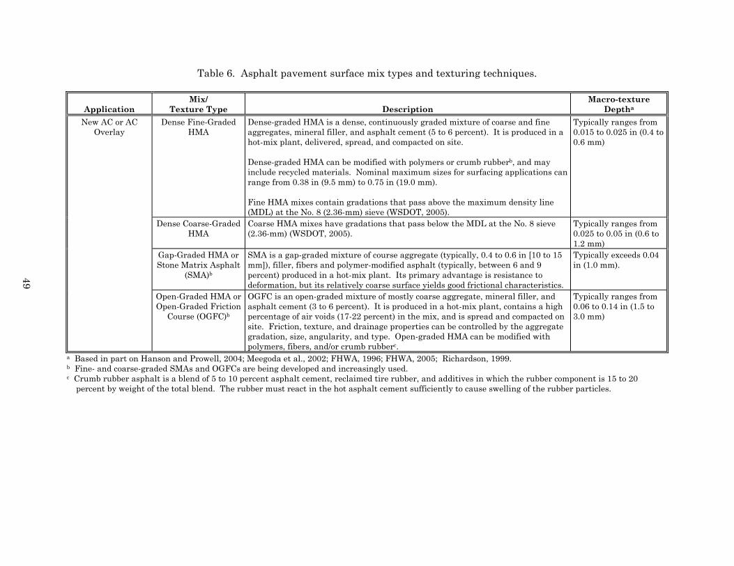
49

Table 6. Asphalt pavement surface mix types and texturing techniques.

Application

Mix/ Texture Type

Description

Macro-texture Deptha

Dense Fine-Graded HMA

Dense-graded HMA is a dense, continuously graded mixture of coarse and fine aggregates, mineral filler, and asphalt cement (5 to 6 percent). It is produced in a hot-mix plant, delivered, spread, and compacted on site. Dense-graded HMA can be modified with polymers or crumb rubberb, and may include recycled materials. Nominal maximum sizes for surfacing applications can range from 0.38 in (9.5 mm) to 0.75 in (19.0 mm). Fine HMA mixes contain gradations that pass above the maximum density line (MDL) at the No. 8 (2.36-mm) sieve (WSDOT, 2005).

Typically ranges from 0.015 to 0.025 in (0.4 to 0.6 mm)

Dense Coarse-Graded HMA

Coarse HMA mixes have gradations that pass below the MDL at the No. 8 sieve (2.36-mm) (WSDOT, 2005).

Typically ranges from 0.025 to 0.05 in (0.6 to 1.2 mm)

Gap-Graded HMA or Stone Matrix Asphalt

(SMA)b

SMA is a gap-graded mixture of course aggregate (typically, 0.4 to 0.6 in [10 to 15 mm]), filler, fibers and polymer-modified asphalt (typically, between 6 and 9 percent) produced in a hot-mix plant. Its primary advantage is resistance to deformation, but its relatively coarse surface yields good frictional characteristics.

Typically exceeds 0.04 in (1.0 mm).

New AC or AC Overlay

Open-Graded HMA or Open-Graded Friction

Course (OGFC)b

OGFC is an open-graded mixture of mostly coarse aggregate, mineral filler, and asphalt cement (3 to 6 percent). It is produced in a hot-mix plant, contains a high percentage of air voids (17-22 percent) in the mix, and is spread and compacted on site. Friction, texture, and drainage properties can be controlled by the aggregate gradation, size, angularity, and type. Open-graded HMA can be modified with polymers, fibers, and/or crumb rubberc.

Typically ranges from 0.06 to 0.14 in (1.5 to 3.0 mm)

a Based in part on Hanson and Prowell, 2004; Meegoda et al., 2002; FHWA, 1996; FHWA, 2005; Richardson, 1999. b Fine- and coarse-graded SMAs and OGFCs are being developed and increasingly used. c Crumb rubber asphalt is a blend of 5 to 10 percent asphalt cement, reclaimed tire rubber, and additives in which the rubber component is 15 to 20 percent by weight of the total blend. The rubber must react in the hot asphalt cement sufficiently to cause swelling of the rubber particles.

50

Table 6. Asphalt pavement surface mix types and texturing techniques (continued).

Application

Mix/ Texture Type

Description

Macro-texture Deptha

Chip Seal Thin surface treatment containing single-sized, high-quality, angular aggregates (0.38 to 0.63 in [9.5 to 15 mm]), spread over and rolled into a liquid asphalt or asphalt emulsion binder. Aggregates are sometimes pre-coated with asphalt emulsion prior to spreading. Completed surface is somewhat coarse, yielding good frictional characteristics.

Typically exceeds 0.04 in (1 mm).

Slurry Seal Slurry mixtures of fine aggregate, mineral filler, and asphalt emulsion. They are similar to micro-surfacing, without interlocking aggregates. Polymers are not always used in the emulsion. Their surface is typically gritty.

Typically range from 0.01 to 0.025 in (0.3 to 0.6 mm).

Micro-Surfacing (polymer-modified

slurry seal)

A slurry mixture containing high-quality crushed, dense-graded aggregate, mineral filler, and polymer-modified asphalt emulsion. It is placed over a tack coat and is capable of being spread in variable thickness layers for rut-filling, correction courses, and wearing course applications.

Typically range from 0.02 to 0.04 in (0.5 to 1 mm).

HMA Overlay See HMA surface mixes above. Ultra-Thin Polymer-

Modified Asphalt (e.g., NovaChip)

Thin gap-graded asphalt surfaces placed using specialized equipment immediately over a thick polymer-modified asphalt emulsion membrane. Following slight compaction the surface provides a semi-porous texture.

Typically exceeds 0.04 in (1 mm).

Friction Restoration of Existing AC

Pavement

Epoxied Synthetic Treatment (e.g.,

Italgrip)

A very thin surface treatment consisting of a two-part polymer resin placed on an existing pavement and covered with a man-made aggregate of re-worked steel slag (0.12 to 0.16 in [3 to 4 mm]). The surface is designed to substantially improve the frictional characteristics of pavements.

Typically exceeds 0.06 in (1.5 mm).

Retexturing of Existing AC Pavement

Micro-Milling Milling equipment, consisting of a self-propelled machine with carbide teeth mounted on a rotating drum, typically removes 0.75 to 1.25 in (19 to 32 mm) from the asphalt surface. Spacing of cuts is approximately 0.2 in (5 mm) versus 0.62-in (6-mm) cut of conventional cold-milling machines. Resulting surface has a fine, smooth pattern that gives smoother ride.

Typically exceeds 0.04 in (1 mm)

a Based in part on FHWA, 1996; FHWA, 2005; Hanson and Prowell, 2004; Mockensturm, 2002; Wade et al., 2001; McNerney et al., 2000; HITEC, 2003; Gransberg and James, 2005; Yaron and Nesichi, 2005.

51

Table 7. Concrete pavement surface mix types and texturing techniques.

Application

Mix/ Texture Type

Description

Macro-texture Deptha

Broom Drag (longitudinal or

transverse)

A long-bristled broom is mechanically or manually dragged over the concrete surface in either the longitudinal or transverse direction. Texture properties are controlled by adjusting the broom angle, bristle properties (length, strength, density), and delay behind the paver. Uniform striations approximately 0.06 to 0.12 in (1.5 to 3.0 mm) deep are produced by this method.

Typically ranges from 0.008 to 0.016 in (0.2 to 0.4 mm).

Artificial Turf Drag (longitudinal)

An inverted section of artificial turf is dragged longitudinally over a concrete surface following placement. Texture properties are controlled by raising/lowering the support boom, adding weight to the turf, and delaying application to allow surface hardening. This method produces uniform 0.06 to 0.12 in (1.5 to 3.0 mm) deep surface striations.

Typically ranges from 0.008 to 0.016 in (0.2 to 0.4 mm), but a deep texture (min depth of 0.04 in [1.0 mm]) has been specifiedb.

Burlap Drag (longitudinal)

One or two layers of moistened coarse burlap sheeting are dragged over the concrete surface following placement. Texture properties are controlled by raising/lowering the support boom and adjusting the delay following concrete placement. This method produces uniform 0.06 to 0.12 in (1.5 to 3.0 mm) deep striations in the surface.

Typically ranges from 0.008 to 0.016 in (0.2 to 0.4 mm).

Longitudinal Tine A mechanical assembly drags a wire comb of tines (~ 5 in [127 mm] long and 10 ft [3 m] wide) behind the paver (and usually following a burlap or turf drag). Texture properties are controlled by the tine angle, tine length, tine spacing, and delay for surface curing. Grooves from 0.12 to 0.25 in (3 to 6 mm) deep and 0.12 in (3 mm) wide are produced by this method, typically spaced at 0.75 in (19 mm).

Typically ranges from 0.015 to 0.04 in (0.4 to 1.0 mm).

New PCC or PCC Overlay

Transverse Tine Accomplished using methods similar to longitudinal tining, however, the mechanical assembly drags the wire comb perpendicular to the paving direction. Variations include skewing the tines 9 to 14° from perpendicular and using random or uniform tine spacing from 0.5 to 1.5 in (12 to 38 mm).

Typically ranges from 0.015 to 0.04 in (0.4 to 1.0 mm).

a Based in part on Hoerner et al., 2003; Hoerner and Smith, 2002; FHWA, 1996; FHWA, 2005. b Minnesota Department of Transportation.

52

Table 7. Concrete pavement surface mix types and texturing techniques.

Application

Mix/ Texture Type

Description

Macro-texture Deptha

Diamond Grinding (longitudinal)

A self-propelled grinding machine with a grinding head of gang-mounted diamond sawing blades removes 0.12 to 0.75 in (3 to 19 mm) of cured concrete surface, leaving a corduroy-type surface. Blades are typically 0.08 to 0.16 in (2 to 4 mm) wide and spaced 0.18 to 0.25 in (4.5 to 6 mm) apart, leaving 0.08 to 0.16 in (2 to 4 mm) high ridges. This method is most commonly used to restore surface characteristics of existing pavements, however, in recent years, it has been used to enhance the surface qualities of new PCC pavements or PCC overlays.

Typically ranges from 0.03 to 0.05 in (0.7 to 1.2 mm).

Porous PCC Gap-graded, small-diameter aggregate are combined with cement, polymers, and water to form a drainable surface layer (typically 8 in [200 mm] thick). That surface layer is bonded to the underlying wet or dry dense concrete layer. Texture properties are controlled by aggregate sizes and gradations. Air voids range from 15 to 25 percent.

Typically exceeds 0.04 in (1 mm).

New PCC or PCC Overlay

Exposed Aggregate PCC

A set retarder is applied to the wet concrete surface and the surface is protected for curing. After 12 to 24 hours, the unset mortar is removed to a depth of 0.04 to 0.08 in (1 to 2 mm) using a power broom. The large diameter aggregate is exposed by this process leaving a uniform surface.

Typically exceeds 0.035 in (0.9 mm).

Friction Restoration of Existing PCC

Pavementb

HMA Overlay See HMA surface mixes above.

Diamond Grinding (longitudinal)

See diamond grinding above.

Longitudinal Diamond Grooving

A self-propelled grooving machine saws longitudinal grooves in the road surface about 0.12 to 0.25 in (3 to 6 mm) deep and spaced 0.5 to 1.5 (13 to 38 mm) apart. This method adds macro-texture for drainage but relies on the original surface for micro-texture.

Typically ranges from 0.035 to 0.055 in (0.9 to 1.4 mm).

Transverse Diamond Grooving

Completed in a manner similar to longitudinal diamond grooving, except the grooves are sawn transverse to the travel direction. This method also adds macro-texture and positive drainage for surface water. It relies on the original surface for micro-texture.

Typically ranges from 0.035 to 0.055 in (0.9 to 1.4 mm).

Retexturing of Existing PCC

Pavement

Shot Abrading An automated machine hurls recycled round steel abrasive material at the pavement surface, abrading the surface and/or removing the mortar and sand particles surrounding the coarse aggregate to a depth of up to 0.25 in (6 mm). Texture properties are controlled by adjusting the steel abrasive material velocity and approach angle and by modifying the forward equipment speed.

Typically ranges from 0.025 to 0.05 in (0.6 to 1.2 mm).

a Based in part on Hoerner et al., 2003; Hoerner and Smith, 2002; FHWA, 1996; FHWA, 2005; HITEC, 2003; Rao et al., 1999. b Other treatments, such as micro-surfacing, ultra-thin polymer-modified asphalt, epoxy-bonded laminates, and thin-bonded PCC overlays, have been used but often have structural performance and/or cost issues.

53

1 2 3 4 5 6 7 8 9 10 11 12 13 14 15 16 17 18 19 20

Figure 18. Example illustration of matching aggregate sources and mix types/texturing 21 techniques to meet friction demand. 22

23 24 Once the design categories have been set, aggregate test protocols and mix/texture type 25 options can be developed for each category, along with design friction levels. The test 26 protocol should list the specific tests to be performed and the criteria/parameters to be used. 27 The criteria should be based on established links between historical friction performance 28 and laboratory test data. 29 30 31 4.3 PROJECT-LEVEL DESIGN GUIDELINES 32 33 This section provides information on state-of-the-practice for providing friction on new and 34 restored asphalt and concrete pavements. Although safety over the established pavement 35 design life is the paramount concern, the design process should target a surface that most 36 economically satisfies the following criteria: 37 38

• Adequate levels of micro-texture over the life of the pavement, as produced by sharp, 39 gritty aggregate with low polish and high wear-resistance characteristics. 40

• Adequate levels of macro-texture over the life of the pavement for efficient 41 displacement of water on the pavement surface. 42

• Low levels of splash/spray, noise generation, glare, tire wear, and rolling resistance. 43 44 Project-level friction design entails selecting aggregates and mix types/texturing techniques 45 that satisfy both initial and long-term friction requirements. A five-step process for 46 designing surfaces for new asphalt or concrete pavement, as well as restoration treatments 47 of existing asphalt or concrete pavement, is as follows: 48

Aggregate Sources

Friction Design Category

Agency Aggregate Testing Protocol

Agency Mix Types/ Texturing Techniques

Source A (high polish)

Source B (moderate polish)

Source C (low polish)

Test Criteria 1 > 5 2 < 25 3 > 50 . . . . . . . .

Mix/Texture Type X (low macro-t) Y (moderate macro-t) Z (high macro-t)

Category I Low demand

α ≤ Design Friction < β

Category II Moderate demand

β ≤ Design Friction < χ)

Category III High demand

Design Friction > χ

C–Y C–Z B–Z

C–X B–Y A–Z

B–X A–X A–Y

Agg. Source–Texture Options

54

1 1. Determine design friction level. 2 2. Select aggregates. 3 3. Establish surface mix types and/or texturing techniques. 4 4. Develop construction specifications. 5 5. Formulate design strategies. 6

7 These design steps are described in detail in the sections below. 8 9 4.3.1 Determining Design Friction Level (Step 1) 10 11 For each new construction or restoration project, a design friction level (expressed as F(60) 12 if IFI is used or as FN) must be selected to satisfy agency policy requirements. The selected 13 design level must ensure that adequate amounts of micro-texture and macro-texture are 14 available throughout the design period. 15 16 The selected design level should take into consideration the design levels of individual PFM 17 sections. Either one overall level can be established for the project corresponding to the 18 PFM section with the highest demand, or multiple levels can be used. In the latter case, 19 care must be taken such that the multiple levels do not result in an excessive number of 20 mix types and/or surface textures to be used along the project. 21 22 Once an agency sets the goal for friction for a particular project, the process of selecting 23 aggregates and mix types/texturing techniques that satisfy the design friction level can 24 begin. An initial list of aggregate source–texture options can be derived from the feasible 25 combinations identified previously for each design category (e.g., B-X, A-X, and A-Y for 26 design category I in figure 18). These, and other potential combinations, can be evaluated 27 more thoroughly for adequacy using the IFI model, as described below in step 3. 28 29 4.3.2 Selecting Aggregates (Step 2) 30 31 The most important factor in achieving long-lasting friction is aggregate selection. 32 Aggregates should have the physical, chemical, and mechanical properties needed to satisfy 33 both initial friction design levels and long-term friction requirements. 34 35 Aggregates must comply with the testing requirements established by the agency. 36 Aggregate samples should be tested early in a project to determine their suitability and 37 compliance with specifications. Frequently, two or more aggregate sources must be 38 combined in appropriate percentages to meet project gradation requirements. 39 40 As stated earlier, aggregates comprised of a matrix of both hard and soft minerals will 41 ensure friction durability. Aggregates not meeting the specified test parameters should be 42 rejected (prior to any mix design effort) and either new materials should be considered and 43 tested or a suitable blend of high- and low-polish susceptible aggregates should be 44 identified. 45 46 Micro-texture in asphalt surface mixes is provided by the coarse aggregate surface texture. 47 Coarse aggregates that exhibit “rough sandpaper” surface textures provide higher levels of 48 micro-texture than those with smooth “fine sandpaper” textures. 49

55

1 Micro-texture in concrete surfaces is generally provided by the fine aggregates in the 2 cement mortar/paste (for concrete mixes with exposed aggregates, the surface properties of 3 the coarse aggregate will dictate micro-texture). Fine aggregates that exhibit angular 4 edges and cubical or irregular shapes generally provide higher levels of micro-texture, 5 whereas those with rounded edges or elongated shapes generally produce lower micro-6 texture. 7 8 4.3.3 Establishing Surface Mix Types and/or Texturing Techniques (Step 3) 9 10 Framework for Achieving Design Friction Level 11 12 As discussed earlier in step 1, potential combinations of aggregate source and mix type/ 13 texturing technique can be evaluated in detail using the IFI model (equations 6 through 9). 14 Using DFT(20) as a surrogate for micro-texture and the CTM to get MPD, FR(S) in 15 equation 8 can be set to DFT(20) at S equal to 20 km/hr. Furthermore, substituting 16 equation 6 into equation 8, one gets the following: 17 18 Eq. 21 19 20 Inserting equation 21 into equation 9, adding in the A, B, and C calibration constants 21 (0.081, 0.732, and 0, respectively) for DFT(20) as given in ASTM E 1960, and re-arranging 22 to solve for DFT(20), the following equation is obtained: 23 24 Eq. 22 25 26 Figure 19 is a plot of the above equation. As an example application, consider a project 27 where it is desired that a locked-wheel smooth-tire friction test give a friction number of 40 28 at a speed limit of 60 km/hr. Then F(60) becomes is 40 and equation 22 becomes as follows: 29 30 Eq. 23 31 32 To achieve the design friction level of 40, the pairs of DFT(20) and MPD given in table 8 are 33 needed. The first pair includes a rather high DFT(20) and the last two pairs include high 34 MPD values. Therefore, the second and third pairs containing MPD values of 0.813 and 35 1.524 mm would need to be selected to give the F(60) or FN needed. 36 37 If the polishing characteristics have been measured or are already known, higher levels of 38 micro-texture and/or macro-texture should be selected to meet the required levels at the 39 end of the design life. For example, if the polished DFT(20) (i.e., PSV) and the MPD are 40 satisfactory, then the initial DFT(20) from the test would need to be specified. If the 41 polished DFT(20) is too low and thus requires a MPD that is too high to meet, then a higher 42 DFT(20) or different aggregate is needed to get the required polished DFT(20) at the end of 43 the design life. 44 45

)7.892.146020(

)20()60( MPDeDFTFR ×+−

×=

( )[ ] )7.892.142060(

732.0/0081.0)60()20( MPDeMPDFDFT ×+−

××−−=

( )[ ] )7.892.14

40(732.0/081.040)20( MPDeDFT ×+×−=

56

1 2 3 4 5 6 7 8 9 10 11 12 13 14 15 16 17 18 19 20 21 22

Figure 19. Example of determining DFT(20) and MPD needed to achieve design friction 23 level. 24

25 26 27

Table 8. Pairs of MPD and DFT(20) needed to achieve design friction level of 40. 28 29

MPD, mm 0.457 0.813 1.524 2.921 4.343 DFT(20) 112.5 86.3 71.1 63.0 60.2

30 31 This method is then a guide for evaluating the levels of micro-texture (DFT(20)) and macro-32 texture (MPD) needed to achieve the design friction level established for a project. It can be 33 used directly in identifying a suitable combination(s) of aggregate and mix type/texturing 34 technique for a project or it can serve as a framework for agencies interested in developing 35 their own customized procedure. It should also be noted that a similar process utilizing the 36 combination of BPN (micro-texture) and MTD (macro-texture) could be established and 37 used. 38 39 During the mix design stage of an asphalt project, there may become the need to “fine-tune” 40 the gradation of a mix to satisfy the friction design requirement. A method for doing this 41 was developed by Sullivan (2005). This method, illustrated in figure 20, uses PSV and 42 MPD to compute IFI (as given in ASTM E 1960) and subsequently determine the design 43 vehicle stopping distance. Figure 21 shows an example vehicle response chart for a selected 44 speed of 50 mi/hr (80 km/hr). 45 46

0

20

40

60

80

100

120

140

160

20 25 30 35 40 45 50 55

F(60) or FN

DFT

(20)

0.457

0.813

1.524

2.921

4.343

MPD, mm

57

1 2 3 4 5 6 7 8 9 10 11 12 13 14 15 16 17 18 19 20 21 22 23 24 25 26 27 28

Figure 20. Flowchart illustration of asphalt pavement friction design methodology 29 (Sullivan, 2005). 30

31 32 33 34 35 36 37 38 39 40 41 42 43 44 45 46 47

Figure 21. Illustration of vehicle response as function of PSV and MPD (Sullivan, 2005). 48 49

Polished Aggregate Friction Value

Des

ign

Veh

icle

Sto

ppin

g D

ista

nce,

m

MPD = 0.2 mm

0.4 mm

0.65 mm 1.2 mm

2.0 mm

350

300

250

200

150

100

50

010 20 30 40 50 60 70 80 90 100

58

1 The Sullivan method uses an equation for computing the MPD based on key asphalt mix 2 characteristics (maximum aggregate size, gradation, binder content). While historical data 3 on asphalt surface mix textures can be used in this process, the MPD equation (derived 4 using comprehensive mix design and surface texture data from the NCAT test track) gives 5 the mix designer greater flexibility in establishing a mix design that will meet friction 6 requirements. 7 8 Although a similar process for conventional concrete mixes could be developed, it is not as 9 important, since the macro-texture is designed separately from the micro-texture. 10 However, agencies are encouraged to quantify the macro-texture (MPD or MTD) of both 11 newly applied and in-service surface texturings (e.g., tined, grooved, or ground surfaces 12 with different groove dimensions, spacings, and orientations), so as to ensure the right 13 supplement for the chosen fine aggregate, 14 15 Asphalt Mix Design 16 17 Mix design requirements for asphalt mixes may vary depending on the nature of the mix 18 type (dense-graded, OGFC, SMA, etc.). The standard agency procedures for mix design 19 should be followed for a given mix type and design requirement. 20 21 During the mix design process, the agency must ascertain the aggregate micro-texture, 22 either through aggregate source historical PSV test data or through testing of the chosen 23 aggregate. The agency must also ascertain the expected in-place macro-texture of the mix, 24 so that a determination can be made as to whether the mix will meet the friction design 25 requirements. Historical mean texture/profile depths (MTD/MPDs), theoretical 26 MTD/MPDs using established relationships, or laboratory-derived MTD/MPDs (using 27 molded samples and performing texture tests) are all possible means for identifying the mix 28 macro-texture. 29 30 Concrete Mix Design and Texturing Selection 31 32 The strength/abrasion properties of the cement mortar/paste largely determine the wearing 33 characteristics of new concrete surfaces, while the coarse aggregate polishing 34 characteristics define restored concrete macro-texture durability. Increasing the cement 35 content (or decreasing the water cement ratio) and implementing sound construction 36 practices maximizes cement paste/mortar strength and, thus, abrasion resistance. 37 38 Concrete surface macro-texture is determined by the texturing type applied. Designers 39 must select feasible surface types that meet macro-texture design requirements. Extensive 40 recommendations for applying the finishing methods listed in table 7 have been presented 41 in several references, including FHWA Technical Advisory T 5040.36 (FHWA, 2005). The 42 recommendations provided can be used to enhance macro-texture for the texturing method 43 selected. 44 45 4.3.4 Development of Construction Specifications (Step 4) 46 47 All agencies have standard specifications for construction of pavement surfaces that provide 48 guidance on requirements for aggregates, mixes, handling, placement, compaction, curing, 49

59

and protection of new surfaces. For some agencies, these specifications do not specifically 1 address friction properties of the wearing surface. To ensure quality friction on new or 2 rehabilitated pavement surfaces, requirements for aggregate properties and test methods 3 presented in this section may be included in project specifications, as needed. 4 5 Special Provisions 6 7 Each project has unique requirements because of the design and construction constraints 8 and special demands. Items such as aggregate blending, noise mitigation, and QA should 9 be clarified in the special provisions of the construction documents and specifications. 10 11 Blending 12 13 Frequently, aggregates from two or more sources must be blended to meet the specification 14 limits. Several studies have reported that the blended aggregate properties tend to be the 15 same as the weighted average of the properties of the individual aggregates (Liang, 2003). 16 Thus, the goal of blending aggregate is to set the percentages of each aggregate used such 17 that the final blend has properties that lies within the specification limits of the tests to be 18 performed. 19 20 Quality Assurance 21 22 Among other things, a QA program often stipulates the frequency of testing aggregate 23 sources. While no specific guidance on the extent and frequency of testing is provided in 24 this Guide, it is strongly suggested that an aggregate source be tested extensively whenever 25 substantially new aggregate deposits are to be used for pavement surfacing. The extent 26 and frequency can be reduced as the agency becomes more familiar with the aggregate 27 source and there is a history of performance for aggregates from the given source (Folliard 28 and Smith, 2003). 29 30 Construction Issues 31 32 Construction deficiencies and poor construction practices can contribute to inadequate 33 friction. Construction issues involve control of aggregate and mix quality during 34 production, handling, stockpiling, mixing, placing, and finishing. Friction restoration 35 treatments in particular, such as chip seals, slurry seals, micro-surfacing, and proprietary 36 surfaces, are susceptible to providing less than expected friction, if poor construction 37 practices are employed. 38 39 4.3.5 Formulation of Design Strategies (Step 5) 40 41 Both monetary and non-monetary factors are considered in selecting preferred pavement 42 design strategy the various feasible alternatives. The main inputs required are (a) 43 estimates of costs, (b) estimates of benefits (if the benefit cost option is selected, not that 44 benefit cost analysis is required only if there is a significant difference in benefits between 45 alternatives, and (c) non-monetary factors. 46 47

60

Important cost elements related to the inclusion of surface friction in the design strategy 1 are: 2 3

• Agency costs. 4 Additional design and engineering costs. 5 Aggregate materials with required frictional properties. 6 Additives, including polymers, to improve surface properties and performance. 7 Frequency/duration of restoration activities. 8

Design strategies involving frequent M&R are typically more costly overall 9 because of the effects of highway user delay costs, traffic control, and so on. 10

Timing of M&R can significantly escalate costs if M&R to restore surface 11 friction does not coincide with M&R to restore structural capacity. 12

13 • User costs 14

Travel delays (time/delay) for friction restoration impact life cycle cost. 15 Friction can adversely influence pavement–tire factors such as tire wear, rolling 16

resistance, and fuel consumption. 17 Safety associated factors that impact crash costs. 18

Frequency of crashes. 19 Value of crashes. 20

21 Benefits from ensuring adequate levels of friction throughout the pavement life are 22 quantified through: 23 24

• Improved highway safety (i.e., reduction in crash costs). 25 Value of lives saved. 26 Value of injuries avoided (medical, loss income, psychological damage). 27 Savings in pain and suffering of crash victims and their families due to a 28

reduction in crashes. 29 Reductions in property damage due to reduction in crashes. 30

31 Non-monetary factors can be included in the decision matrix and addressed through (a) 32 agency policies and criteria on these factors and (b) appropriate weights to these factors to 33 reflect the importance assigned to them by the agency. The non-monetary design 34 considerations include (AASHTO, 1993): 35 36

• Service life. 37 • Duration of construction. 38 • Traffic control problems. 39 • Reliability, constructability, and maintainability of design. 40

41 Non-monetary considerations associated with pavement friction include: 42 43

• Pavement–tire noise. 44 • Splash and spray. 45 • Fuel consumption/rolling resistance. 46 • Tire wear. 47 • Reflectance and glare. 48

61

REFERENCES 1 2 3 American Association of State Highway and Transportation Officials (AASHTO). 1976. 4 Guidelines for Skid Resistant Pavement Design, Prepared by the Task Force for Pavement 5 Design of the AASHTO Operating Subcommittee on Design, Washington, D.C. 6 7 American Association of State Highway and Transportation Officials (AASHTO). 1993. 8 Guide for Design of Pavement Structures, AASHTO, Washington, D.C. 9 10 American Association of State Highway and Transportation Officials (AASHTO). 2001. “A 11 Policy on Geometric Design of Highways and Streets,” AASHTO Green Book, AASHTO, 12 Washington, D.C. 13 14 Agent, K.R., N. Stamatiadis, and S. Jones. 1996. “Development of Accident Reduction 15 Factors,” Research Report KTC-96-13, University of Kentucky, Kentucky Transportation 16 Cabinet, Lexington, Kentucky. 17 18 Anderson, D.A., R.S. Huebner, J.R. Reed, J.C. Warner, and J.J. Henry. 1998. Improved 19 Surface Drainage of Pavements, NCHRP Web Document 16, National Cooperative Highway 20 Research Foundation (NCHRP), Washington, D.C. 21 22 Austroads. 2005. “Guidelines for the Management of Road Surface Skid Resistance,” 23 Austroads Publication No. AP-G83/05, Austroads Incorporated, Sydney, Australia. 24 25 Dahir, S.H. and J.J. Henry. 1978. Alternatives for the Optimization of Aggregate and 26 Pavement Properties Related to Friction and Wear Resistance, Report No. FHWA-RD-78-27 209, Federal Highway Administration (FHWA), Washington, D.C. 28 29 Federal Highway Administration (FHWA). 1979. “Texturing and Skid Resistance of 30 Concrete Pavements and Bridge Decks,” Technical Advisory T 5140.10, U.S. Department of 31 Transportation, FHWA, Washington, D.C. 32 33 Federal Highway Administration (FHWA). 1980. “Skid Accident Reduction Program,” 34 Technical Advisory T 5040.17, U.S. Department of Transportation, FHWA, Washington, 35 D.C. 36 37 Federal Highway Administration (FHWA). 1996. “PCC Surface Texture Technical 38 Working Group Findings,” FHWA, Washington, D.C. 39 40 Federal Highway Administration (FHWA). 2005. “Surface Texture for Asphalt and 41 Concrete Pavements,” Technical Advisory T 5040.36, U.S. Department of Transportation, 42 Federal Highway Administration, Washington, D.C. 43 44 Flintsch, G.W., E. de Leon, K.K. McGhee, and I.L. Al-Qadi. 2003. “Pavement Surface 45 Macro-texture Measurement and Application, Paper presented at 82nd Annual Meeting of 46 the Transportation Research Board, Washington, D.C. 47 48

62

Folliard, K.J. and K.D. Smith. 2003. “Aggregate Tests for Portland Cement Concrete 1 Pavements: Review and Recommendations,” September edition (No. 281) of NCHRP 2 Research Results Digest, National Cooperative Highway Research Program (NCHRP), 3 Washington, D.C. 4 5 Glennon, J.C. 1996. “Roadway Defects and Tort Liability,” Lawyers & Judges Publishing 6 Company, Inc., Tucson, Arizona. 7 8 Gransberg, D. and D.M.B. James. 2005. “Chip Seal Best Practices,” NCHRP Synthesis 9 342, National Cooperative Highway Research Program (NCHRP), Washington, D.C. 10 11 Hanson, D.I. and B.D. Prowell. 2004. “Evaluation of Circular Texture Meter for Measuring 12 Surface Texture of Pavements,” NCAT Report No. 04-05, National Center for Asphalt 13 Technology (NCAT), Auburn, Alabama. 14 15 Henry, J.J. 1983. “Comparison of Friction Performance of a Passenger Tire and the ASTM 16 Standard Test Tires, ASTM STP 793, ASTM, Philadelphia, Pennsylvania. 17 18 Henry, J.J. 2000. “Evaluation of Pavement Friction Characteristics—A Synthesis of 19 Highway Practice,” NCHRP Synthesis 291, Transportation Research Board, Washington, 20 D.C. 21 22 Highways Agency (HA). 2005. Design Manual for Roads and Bridges, Volume 7, HD 28, 23 “Skid Resistance,” Department for Transport, London, United Kingdom. 24 25 Highway Innovative Technology Evaluation Center (HITEC). 2003. Evaluations—Italgrip 26 System, Civil Engineering Research Foundation (CERF) HITEC website 27 (www.cerf.org/hitec/evals.htm), Washington D.C. 28 29 Hoerner, T.E., K.D. Smith, R.M. Larson, and M.E. Swanlund. 2003. “Current Practice of 30 PCC Pavement Texturing,” Paper presented at 82nd Annual Meeting of the Transportation 31 Research Board, Washington, D.C. 32 33 Hoerner, T.E. and K.D. Smith. 2002. High Performance Concrete Pavement: Pavement 34 Texturing and Tire-Pavement Noise, FHWA Report No. FHWA-IF-02-020, Federal Highway 35 Administration, Washington, D.C. 36 37 Horne, W.B. and F. Buhlmann. 1983. “A Method for Rating the Skid Resistance and 38 Micro/Macro-texture Characteristics of Wet Pavements,” ASTM International STP No. 793, 39 W. E Meyers and J. D. Walter, Editors American Society for testing and materials, 40 Philadelphia, Pennsylvania. 41 42 Ivey, D.L., L.I. Griffin III, J.R. Lock, and D.L. Bullard. 1992. “Texas Skid Initiated 43 Accident Reduction Program,” Final Report, Research Report 910-1F, TTI: 2-18-89/910, TX-44 92/910-1F, Texas Department of Transportation, Austin, Texas. 45 46

63

Kandhal, P.S., F. Parker Jr., and R.B. Mallick. 1997. Aggregate Tests for Hot Mix Asphalt: 1 State of the Practice, NCAT Report No. 97-6, National Center for Asphalt Technology 2 (NCAT), Auburn, Alabama. 3 4 Kandhal, P.S. and F. Parker Jr. 1998. “Aggregate Tests Related to Asphalt Concrete 5 Performance in Pavements,” NCHRP Report 405, National Cooperative Highway Research 6 Program (NCHRP), Washington, D.C. 7 8 Kuemmel, D.A., R.C. Sonntag, J. Crovetti, and Y. Becker. 2000. “Noise and Texture on 9 PCC Pavements: Results of a Multi-State Study,” Final Report No. WI/SPR-08-99, 10 Wisconsin Department of Transportation, Madison, Wisconsin. 11 12 Larson, R.M. 1999. “Consideration of Tire/Pavement Friction/Texture Effects on Pavement 13 Structural Design and Materials Mix Design,” Federal Highway Administration, Office of 14 Pavement Technology, Washington, D.C. 15 16 Liang, R.Y. 2003. “Blending Proportions of High Skid and Low Skid Aggregate,” Final 17 Report prepared for Ohio Department of Transportation (ODOT), Columbus, Ohio. 18 19 Liang, R.Y. and L.L. Chyi. 2000. “Polishing And Friction Characteristics Of Aggregates 20 Produced in Ohio,” Report No. FHWA/OH-2000/001, Ohio Department of Transportation, 21 Columbus, Ohio. 22 23 Mahone, D.C. and S.N. Runkle. 1972. “Pavement Friction Needs,” Highway Research 24 Record 396, Highway Research Board, Washington D.C. 25 26 McCullough, B.F. and K.D. Hankins. 1966. “Skid Resistance Guidelines for Surface 27 Improvements on Texas Highways,” Highway Research Record 131, Highway Research 28 Board, Washington D.C. 29 30 McGhee, K.K. and G.W. Flintsch. 2003. “High Speed Texture Measurement of 31 Pavements,” Report No. VTRC 03-R9, Virginia Transportation Research Council (VTRC), 32 Charlottesville, Virginia. 33 34 McNerney, M.T., B.J. Landsberger, T. Turen, and A. Pandelides. 2000. “Comparative Field 35 Measurements of Tire/Pavement Noise of Selected Texas Pavements,” Report No. 36 FHWA/TX-7-2957-2, Texas Department of Transportation, Austin, Texas. 37 38 Meegoda, J.N., C.H. Hettiarachchi, G.M. Rowe, N. Bandara, and M.J. Sharrock. 2002. 39 Correlation of Surface Texture, Segregation, and Measurement of Air Voids, Final Report 40 prepared for New Jersey Department of Transportation, Trenton, New Jersey. 41 42 Meininger, R. C. 1994. “Degradation Resistance, Strength, Toughness, and Related 43 Properties,” ASTM STP 169C, ASTM, West Conshohocken, Pennsylvania. 44 45 Meyer, W.E. 1982. Synthesis of Frictional Requirements Research, Report No. FHWA/RD-46 81/159, Federal Highway Administration (FHWA), Washington, D.C. 47 48

64

Mockensturm, E.M., B.T. Kulakowski, and N.M. Hawk. 2002. “Measurement and 1 Evaluation of Roadside Noise Generated by Transit Buses,” Final Report, The Institute for 2 Safe, Quiet, and Durable Highways (ISQDH), Purdue University. 3 4 Moyer, R.A. 1959. “Historical Background of Skid Resistance Measurement—American 5 Experience,” 1st International Skid Prevention Conference, Charlottesville, Virginia. 6 7 National Highway Traffic Safety Administration [NHTSA]. 1998. “Report to Congress: 8 Update on the Status of Splash and Spray Suppression Technology for Large Trucks,” 9 NHTSA, Washington, D.C. 10 11 NHTSA. 2004. Traffic Safety Facts 2003 – A Compilation of Motor Vehicle Crash Data 12 from the Fatality Analysis Reporting System and the General Estimates System, NHTSA 13 website (http://www-nrd.nhtsa.dot.gov.) 14 15 Noyce, D.A., H.U. Bahia, J.M. Yambo, and G. Kim. 2005. Incorporating Road Safety into 16 Pavement Management: Maximizing Asphalt Pavement Surface Friction for Road Safety 17 Improvements,” Draft Literature Review and State Surveys, Midwest Regional University 18 Transportation Center (UMTRI), Madison, Wisconsin. 19 20 Ong, G.P. and T.F. Fwa. 2006. “Transverse Pavement Grooving Against Hydroplaning I: 21 Simulation Model,” Journal of Transportation Engineering, Volume 132, Number 6, 22 American Society of Civil Engineers (ASCE), Reston, Virginia. 23 24 Page, B.G. and L.F. Butas. 1986. Evaluation of Friction Requirements for California State 25 Highways in Terms of Highway Geometrics, Report No. FHWA/CA/TL 86/01, Federal 26 Highway Administration, Washington, D.C. 27 28 Permanent International Association of Road Congresses (PIARC). 1987. “Report of the 29 Committee on Surface Characteristics,” Proceedings of the 18th World Road Congress, 30 Brussels, Belgium. 31 32 Permanent International Association of Road Congresses (PIARC). 1995. International 33 PIARC Experiment to Compare and Harmonize Texture and Skid Resistance Measurements, 34 Report AIPCR- 01.040.T-1995, PIARC, Brussels, Belgium. 35 36 Prowell, B.D., J. Zhang, and E.R. Brown. 2005. “Aggregate Properties and the 37 Performance of SuperPave-Designed Hot Mix Asphalt,” NCHRP Report 539, National 38 Cooperative Highway Research Program (NCHRP), Washington, D.C. 39 40 Rado, Z. 1994. “Analysis of Texture Models,” PTI Report No. 9510, Pennsylvania 41 Transportation Institute, Penn State University, State College, Pennsylvania. 42 43 Radlinski, R.W. and S.F. Williams. 1985. “Stopping Capability of Air-Braked Vehicles,” 44 Report No. DOT-HS-806-738, NHTSA Heavy Duty Vehicle Brake Research Program, 45 National Highway Traffic Safety Administration (NHTSA), Washington, D.C. 46 47

65

Radt, H.S. and W.F. Milliken. 1960. Motions of Skidding Automobiles, Paper No. 600133 1 (205A), Society of Automotive Engineers (SAE), Warrendale, Pennsylvania. 2 3 Rao, S., H.T. Yu, L. Khazanovich, M.I. Darter, and J.W. Mack. 1999. “Longevity of 4 Diamond Ground Concrete Pavements,” Paper presented at 78th Annual Meeting of the 5 Transportation Research Board, Washington, D.C. 6 7 Richardson, J.T.G. 1999. “Stone Mastic Asphalt in the U.K.,” Society of Chemical Industry 8 (SCI) Lecture Papers Series, London, United Kingdom. 9 10 Rizenbergs, R.L., J.L. Burchett, and C.T. Napier. 1973. Accidents on Rural Interstate and 11 Parkway Roads and Their Relation to Pavement Friction, Kentucky Department of 12 Transportation, Frankfort, Kentucky. 13 14 Sandburg, U. 1998. “Influence of Road Surface Texture on Traffic Characteristics Related 15 to Environment, Economy, and Safety: A State-of-the-Art Study Regarding Measures and 16 Measuring Methods,” VTI Report 53A-1997, Swedish National Road Administration, 17 Borlange, Sweden. 18 19 Sandburg, U. and J.A. Ejsmont. 2002. Tyre/Road Noise Reference Book, ISBN 91-631-20 2610-9, Informex, Kisa, Sweden. 21 22 Sullivan, B.W. 2005. “Development of a Fundamental Skid Resistance Asphalt Mix Design 23 Procedure,” Pavement Management Service, Sydney, Australia. 24 25 Viner H., R. Sinhal, and T. Parry. 2004. “Review of UK Skid Resistance Policy,” Paper 26 prepared for 5th International Symposium on Pavement Surface Characteristics---Road and 27 Airports, Toronto, Ontario, Canada. 28 29 Wade, M., R. DeSombre, and D. Peshkin. 2001. “High Volume/High Speed Asphalt 30 Roadway Preventive Maintenance Surface Treatments,” Final Report, South Dakota 31 Department of Transportation, Pierre, South Dakota. 32 33 Wallman, C.G. and H. Astrom. 2001. “Friction Measurement Methods and the Correlation 34 Between Road Friction and Traffic Safety,” Swedish National Road and Transport Research 35 Institute, VTI Meddelande 911A, Linkoping, Sweden. 36 37 Wambold, J.C., J.J. Henry, and R.R. Blackburn. 1984. Pavement Surface Texture: 38 Significance and Measurement, Report No. FHWA/RD-84/092, Federal Highway 39 Administration, Washington, D.C. 40 41 Washington Department of Transportation (WSDOT). 2005. “Factors Affecting HMA 42 Permeability,” Tech Notes, WSDOT Materials Laboratory, Olympia, Washington. 43 44 World Health Organization (WHO). 2004. “World Report on Road Traffic Injury 45 Prevention,” WHO, Geneva, Switzerland. 46 47

66

Wu, Y., F. Parker, and K. Kandhal. 1998. Aggregate Toughness/Abrasion Resistance and 1 Durability/Soundness Tests Related to Asphalt Concrete Performance in Pavements, NCAT 2 Report 98-04, National Center for Asphalt Technology (NCAT), Auburn, Alabama. 3 4 Yaron, R. and S. Nesichi. 2005. “Alleviating the Skid Resistance Problem: The Israeli 5 Experience,” Paper presented at First International Conference on Surface Friction: Roads 6 and Runways, Christchurch, New Zealand. 7 8

This page intentionally left blank. 1 2 3 4 5 6

1 2 3 4 5 6 7 8 9 10 11 12 13 14 15 16 17 18 19 20

APPENDIX A. TERMINOLOGY 21 22

This page intentionally left blank. 1 2 3

A-1

ABBREVIATIONS AND ACRONYMS 1 2 3 ABS Anti-lock Braking System 4 AC Asphalt Concrete 5 ADT Average Daily Traffic 6 AIR Acid Insoluble Residue test 7 ASTM American Society for Testing and Materials 8 BPN British Pendulum Number 9 BPT British Pendulum Tester 10 CEN European Committee for Standardization 11 CSA Canadian Standards Association 12 CTM Circular Texture Meter 13 DFT Dynamic Friction Tester 14 ETD Estimated Mean Texture Depth 15 FARS Fatality Analysis Reporting System 16 FN Friction Number 17 HMA Hot-Mix Asphalt 18 HPS (Critical) Hydroplaning Speed 19 ICM Integrated Climatic Model 20 IFI International Friction Index 21 ISO International Standards Organization 22 IVS Intelligent Vehicle System 23 LCCA Life-Cycle Cost Analysis 24 MPD Mean Profile Depth 25 MTD Mean Texture Depth 26 MUTCD Manual on Uniform Traffic Control Devices 27 M&R Maintenance and Rehabilitation 28 OFM Outflow Meter 29 OFT Outflow Time 30 OGFC Open-Graded Friction Courses 31 PCC Portland Cement Concrete 32 PFM Pavement Friction Management 33 PMS Pavement Management System 34 PSV Polished Stone Value 35 QA Quality Assurance 36 QC Quality Control 37 ROSANV Road Surface Analyzer 38 SFT Surface Friction Tester 39 SMA Stone Matrix Asphalt 40 SPM Sand Patch Method 41 SSD Stopping Sight Distance 42 TDG Texture Depth Gauge 43 WCR Wet Crash Rate 44 WFT Water Film Thickness 45 WSR Wet Skidding Rate 46 47 48

A-2

TERM DEFINITIONS 1 2 3 Adhesion—Frictional forces that result from the small-scale bonding/interlocking of the 4 vehicle tire rubber and the pavement surface as they come in contact with each other. 5 6 Anti-lock Braking System (ABS)—A collection of sensing and control hardware installed on 7 a vehicle to prevent wheel lock-up during brake application. 8 9 Braking Force Coefficient—The ratio of tire braking force to normal force. 10 11 Braking Force Coefficient, Peak—The maximum value of tire braking force coefficient that 12 occurs prior to wheel lockup as the braking torque is progressively increased. 13 14 Braking Force Coefficient, Slide—The value of tire braking force coefficient obtained on a 15 locked wheel. 16 17 Coefficient of Friction—The ratio of the value of the tangential force between the tire tread 18 rubber and the horizontal traveled surface to the absolute value of normal force attainable 19 on a given traveled surface on a given rolling or locked wheel at specified test conditions. 20 21 Contact Area—The gross tire contact area that is loaded under static conditions against a 22 smooth flat surface. 23 24 Cornering Force—The horizontal force acting perpendicularly to the instantaneous motion 25 vector of the center of contact for a tire operating at a slip angle. 26 27 Critical Slip Angle—The value of the tire slip angle at the peak cornering force coefficient. 28 29 Friction Number (sometimes referred to as Skid Number)—The number that is used to 30 report the results of a pavement friction test conducted in accordance with ASTM Test 31 Method E 274; usually expressed as the friction coefficient multiplied by 100. 32 33 Hydroplaning—Phenomenon in which a vehicle tire is separated from the pavement surface 34 by the water pressure that builds up at the pavement–tire interface. 35 36 Hysteresis—Frictional forces resulting from the energy loss due to bulk deformation of the 37 vehicle tire. 38 39 International Friction Index (IFI)—Friction index defined by two parameters, a calibrated 40 friction value at 37 mi/hr (60 km/hr), F(60), and the speed gradient, SP. 41 42 Intervention Level—The point in a friction deterioration curve where an agency must either 43 take immediate corrective action, such as applying a restorative treatment, or provide 44 proper cautionary measures, such as posting “Slippery When Wet” signs and/or reduced 45 speed signs. 46 47

A-3

Investigatory Level—The point in a friction deterioration curve where an agency should 1 start more carefully monitoring the friction and/or crash levels at a particular site and 2 begin the process of planning for some sort of restorative action. 3 4 Pavement Friction Management (PFM)—A systematic approach to minimizing skid-crashes 5 through friction and/or crash rate monitoring, timely application of friction restoration 6 treatments, and utilization of good friction design and construction practices. 7 8 Pavement–Tire Friction (or Pavement Friction)—The force that resists the relative motion 9 between a vehicle tire and a pavement surface. A measure of this resistive force is the non-10 dimensional friction coefficient, µ. 11 12 Side-Force Friction—The friction that develops as a vehicle changes direction or 13 compensates for pavement cross-slope and/or wind effects. 14 15 Skid Resistance—The ability of the traveled surface to prevent the loss of tire traction. 16 17 Slip Angle—The angle between the X-axis and the direction of travel at the center of tire 18 contact. 19 20 Slip Speed—The difference between the speed of the axis of the measuring wheel, which is 21 equal to the traveling speed of the measuring device, and the tangential velocity of 22 measuring wheel with unloaded radius. 23 24 Splash—The large droplets of water that are thrown off the tire or squeezed out from 25 pavement–tire contact area. Splash is associated with large water depths or low vehicle 26 speeds. 27 28 Spray—The mist that is carried alongside and thrown behind a moving vehicle by the 29 turbulent airflow created by the vehicle, other nearby vehicles, and wind. Spray is 30 associated with shallow water depths or high vehicle speeds. 31 32 33 SYMBOLS 34 35 A Surface texture amplitude.

BPN British Pendulum Number

CD Coefficient of displacement drag.

COV Coefficient of variation.

Ĉ Shape factor in the Rado friction model (log normal).

DFT Dynamic Friction Test index.

EMTD Estimated mean texture depth.

F Friction force between vehicle tire and pavement surface.

FA Adhesion component of pavement friction.

FH Hysteresis component of pavement friction.

A-4

FS Side-force friction.

FW Applied vertical force on a wheel axle, equal to the device mass multiplied by the gravity constant, or a controlled vertically applied force.

Fx Brake force. Fy Lateral force. FN(##) Friction number FN##R, SN##R

Friction number/skid number determined at ## mi/hr using a ribbed tire.

FN##S, SN##S

Friction number/skid number determined at ## mi/hr using a smooth tire.

FN(##)R, SN(##)R

Friction number/skid number determined at ## km/hr using a ribbed tire.

FN(##)S, SN(##)S

Friction number/skid number determined at ## km/hr using a smooth tire.

F(60) Friction number of the International Friction Index (IFI). HPS Critical hydroplaning speed. IR Excess rainfall (rainfall intensity minus pavement surface permeability). IFI International Friction Index. L Drainage path length. M Mass of vehicle. MPD Mean profile depth. MTD Mean texture depth. P Centripetal force (horizontal). R Radius of curvature of highway curve. S Slip speed. SMAX Critical slip speed value in Rado friction model (log normal friction model). SP Speed number of the International Friction Index (IFI). V Travel speed. VP Average peripheral speed of tire. W Weight of vehicle WFT Water film thickness. e Pavement super-elevation i Rainfall intensity. m Mass of vehicle. n Manning’s roughness coefficient. r Average tire radius. α Angle of super-elevation. λ Surface texture wavelength. μ 1) Friction coefficient as the ratio of a horizontal force to a vertical force in the pavement–tire

contact area. 2) A reported friction value.

μmax Maximum friction value. ω Angular velocity of tire. 1

1 2 3 4 5 6 7 8 9 10 11 12 13 14 15 16 17 18 19

APPENDIX B. STANDARDS RELEVANT TO 20 PAVEMENT FRICTION 21

22 23

This page intentionally left blank. 1 2 3

B-1

1 AASHTO TP 61 Standard Method of Test for Determining the Percentage of Fracture in Coarse Aggregate

AASHTO T 96 Standard Method of Test for Resistance to Degradation of Small-Size Coarse Aggregate by Abrasion and Impact in the Los Angeles Machine

AASHTO T 104 Standard Method of Test for Soundness of Aggregate by Use of Sodium Sulfate or Magnesium Sulfate

AASHTO T 261 Standard Method of Test for Measuring Texture Depth of Portland Cement Concrete Using a Tire Tread Depth Gauge

AASHTO T 278 Standard Method of Test for Surface Frictional Properties Using the British Pendulum Tester

AASHTO T 279 Standard Method of Test for Accelerated Polishing of Aggregates Using the British Wheel

AASHTO T 304 Standard Method of Test for Uncompacted Void Content of Fine Aggregate

AASHTO T 327 (formerly TP 58)

Standard Method of Test for Resistance of Coarse Aggregate to Degradation by Abrasion in the Micro-Deval Apparatus

AASHTO T 326 (formerly TP 56)

Standard Method of Test for Uncompacted Void Content of Coarse Aggregates (as influenced by particle shape, surface texture, and grading)

ASTM C 88 Standard Test Method for Soundness of Aggregate of Use of Sodium Sulfate or Magnesium Sulfate

ASTM C 131 Standard Test Method for Resistance to Degradation of Small-Size Coarse Aggregate by Abrasion and Impact in the Los Angeles Machine

ASTM C 294 Standard Descriptive Nomenclature for Constituents of Concrete Aggregates

ASTM C 295 Standard Guide for Petrographic Examination of Aggregates for Concrete

ASTM C 535 Standard Test Method for Resistance to Degradation of Large-Size Coarse Aggregate by Abrasion and Impact in the Los Angeles Machine

ASTM C 1252 Standard Test Method for Uncompacted Void Content of Fine Aggregate (as Influenced by Particle Shape, Surface Texture, and Grading)

ASTM D 1155 Standard Test Method for Roundness of Glass Spheres (for Sand Patch Method)

ASTM D 3042 Standard Test Method for Insoluble Residue in Carbonate Aggregates

ASTM D 3319 Standard Practice for the Accelerated Polishing of Aggregates Using the British Wheel

ASTM D 5821 Standard Test Method for Determining the Percentage of Fractured Particles in Coarse Aggregate

ASTM D 6928 Standard Test Method for Resistance of Coarse Aggregate to Degradation by Abrasion in the Micro-Deval Apparatus

ASTM E 274 Standard Test Method for Skid Resistance of Paved Surfaces Using a Full-Scale Tire

ASTM E 303 Standard Test Method for Measuring Surface Frictional Properties Using the British Pendulum Tester

ASTM E 501 Standard Specification for Standard Rib Tire for Pavement Skid-Resistance Tests

ASTM E 524 Standard Specification for Standard Smooth Tire for Pavement Skid-Resistance Tests

ASTM E 670 Standard Test Method for Side Force Friction on Paved Surfaces Using the Mu-Meter

ASTM E 965 Standard Test Method for Measuring Pavement Macro-texture Depth Using a Volumetric Technique

ASTM E 1845 Standard Practice for Calculating Pavement Macro-texture Mean Profile Depth (Laser Profiler Method)

B-2

ASTM E 1911 Standard Test Method for Measuring Paved Surface Frictional Properties Using the Dynamic Friction Tester

ASTM E 1960 Standard Practice for Calculating International Friction Index of a Pavement Surface

ASTM E 2157 Standard Test Method for Measuring Pavement Macro-texture Properties Using the Circular Track Meter

ASTM E 2341 Standard Test Method for Determining the Stopping Distance Number by Initia1 Speed and Stopping Distance at Traffic Incident Site

ASTM E 2380 ASTM WK 364

Standard Test Method for Measuring Pavement Texture Drainage Using an Outflow Meter

CSA A23.2-23A Resistance of Fine Aggregate to Degradation by Abrasion in the Micro-Deval Apparatus

1 2 3 4