guide to using multiple regression in excel (mrcx v.1.1) for · pdf file ·...

PNNL-19775, Rev. 1

Prepared for the U.S. Department of Energy under Contract DE-AC05-76RL01830

Guide to using Multiple Regression in Excel (MRCX v.1.1) for Removal of River Stage Effects from Well Water Levels RD Mackley TC Pulsipher FA Spane CH Allwardt September 2010

DISCLAIMER This report was prepared as an account of work sponsored by an agency of the United States Government. Neither the United States Government nor any agency thereof, nor Battelle Memorial Institute, nor any of their employees, makes any warranty, express or implied, or assumes any legal liability or responsibility for the accuracy, completeness, or usefulness of any information, apparatus, product, or process disclosed, or represents that its use would not infringe privately owned rights. Reference herein to any specific commercial product, process, or service by trade name, trademark, manufacturer, or otherwise does not necessarily constitute or imply its endorsement, recommendation, or favoring by the United States Government or any agency thereof, or Battelle Memorial Institute. The views and opinions of authors expressed herein do not necessarily state or reflect those of the United States Government or any agency thereof.

PACIFIC NORTHWEST NATIONAL LABORATORY operated by BATTELLE

for the UNITED STATES DEPARTMENT OF ENERGY

under Contract DE-ACO5-76RL01830

Printed in the United States of America

Available to DOE and DOE contractors from the Office of Scientific and Technical Information,

P.O. Box 62, Oak Ridge, TN 37831-0062; ph: (865) 576-8401 fax: (865) 576 5728

email: [email protected]

Available to the public from the National Technical Information Service, U.S. Department of Commerce, 5285 Port Royal Rd., Springfield, VA 22161

ph: (800) 553-6847 fax: (703) 605-6900

email: [email protected] online ordering: http://www.ntis.gov/ordering.htm

PNNL-19775, Rev. 1

Guide to using Multiple Regression in Excel (MRCX v.1.1) for Removal of River Stage Effects from Well Water Levels RD Mackley TC Pulsipher FA Spane CH Allwardt September 2010 Prepared for the U.S. Department of Energy under Contract DE-AC05-76RL01830 Pacific Northwest National Laboratory Richland, Washington 99352

iii

Summary

A software tool was created in Fiscal Year 2010 (FY11) that enables multiple-regression correction of well water levels for river-stage effects. This task was conducted as part of the Remediation Science and Technology project of CH2M-HILL Plateau Remediation Company (CHPRC). This document contains an overview of the multiple regression convolution/deconvolution methodology and is intended to be a user’s manual for the Multiple Regression in Excel (MRCX) v.1.1 software. This document contains a step-by-step tutorial that shows users how to use MRCX to correct river effects in two different wells.

This report is accompanied by an enclosed CD that contains the MRCX installer application and files used in the tutorial exercises.

v

Acknowledgments

The authors would like to acknowledge the valuable contributions of staff and colleagues who have helped willingly in support of the creation of the MRCX v.1.1 software tool and user’s manual. We would like to thank Kyle R. Parker (PNNL) and Robert S. Edrington (CHPRC) for providing water level data. Special thanks to Matt Tonkin and Rachel Shannon (S.S. Papadopulos & Associates, Inc.) for their instructive technical discussion and willingness to share information and data.

We would like to acknowledge the contributions of technical reviewers, including Vince R. Vermeul, and Megan Peters for editing and text processing (PNNL).

vii

Contents

Summary ............................................................................................................................................... iii

Acknowledgments ................................................................................................................................. v

1.0 Introduction .................................................................................................................................. 1.1

1.1 Groundwater Response to Changes in River Stage .............................................................. 1.1

1.2 Multiple-Regression Correction ........................................................................................... 1.2

1.2.1 Application to River-Stage Effects ............................................................................ 1.2

1.2.2 Multiple-Regression Models Issues .......................................................................... 1.6

2.0 Software Installation and Configuration ....................................................................................... 2.1

2.1 Installing the MRCX v.1.1 Software Files ........................................................................... 2.1

2.2 File Saving and Renaming ................................................................................................... 2.1

2.3 Configuring the MRCX Workbook Template ...................................................................... 2.2

2.3.1 Enabling the MRCX VBA Macro in Excel 2007 ...................................................... 2.2

3.0 User Interface ............................................................................................................................... 3.1

3.1 General Overview ................................................................................................................ 3.1

3.2 Input Data ............................................................................................................................. 3.3

3.2.1 Copy Paste Special-Values ........................................................................................ 3.3

3.2.2 Training Data ............................................................................................................. 3.4

3.2.3 Correction data .......................................................................................................... 3.4

3.2.4 Input Data Requirements ........................................................................................... 3.4

3.3 Model Configuration ............................................................................................................ 3.5

3.3.1 Time Filtering ............................................................................................................ 3.6

3.3.2 Data Value Option ..................................................................................................... 3.6

3.3.3 Lag Option................................................................................................................. 3.7

3.3.4 Maximum Number of Lags ....................................................................................... 3.8

3.3.5 Trend Adjustment ...................................................................................................... 3.9

3.4 Command Buttons ................................................................................................................ 3.11

3.4.1 Reset Filter ................................................................................................................ 3.11

3.4.2 Run Multiple Regression on Training Data .............................................................. 3.11

3.5 Results .................................................................................................................................. 3.12

4.0 Tutorial Examples ......................................................................................................................... 4.1

4.1 Example 1: Well 399-1-21A ............................................................................................... 4.1

4.1.1 Entering the Input Data ............................................................................................. 4.2

4.1.2 Configuring the Multiple Regression Model ............................................................. 4.3

4.1.3 Varying the Maximum Lag Term ............................................................................. 4.4

4.1.4 Different Training and Correction Time Periods ...................................................... 4.5

4.1.5 Batch Lag Mode ........................................................................................................ 4.6

viii

4.2 Example 2: Well 199-K-112A ............................................................................................ 4.7

4.2.1 Input Data .................................................................................................................. 4.9

4.2.2 Establishing a Suitable Training Period and Maximum Lag Combination ............... 4.9

4.2.3 Linear Trend Adjustment .......................................................................................... 4.13

5.0 References .................................................................................................................................... 5.1

ix

Figures

1.1 River-Stage Effects on Well 399-1-21A ....................................................................................... 1.2

1.2 River Response Function for Well 399-1-21A ............................................................................. 1.4

1.3 Observed, Predicted, and Corrected Water Level Results for Well 399-1-21A ........................... 1.6

2.1 Macro Security Warning Notification on the Excel 2007 Toolbar Ribbon .................................. 2.2

2.2 Enabling Temporary Macro Permission ....................................................................................... 2.3

3.1 Generalized MRCX Workflow Process Diagram ......................................................................... 3.2

3.2 Input Data Worksheet ................................................................................................................... 3.3

3.3 Model Config Worksheet .............................................................................................................. 3.5

3.4 Time Filtering Settings ................................................................................................................. 3.6

3.5 Data Value Type Option Configuration Setting ........................................................................... 3.7

3.6 Lag Option Configuration Setting ................................................................................................ 3.8

3.7 Maximum Lag Configuration Setting ........................................................................................... 3.9

3.8 Background Trends in River-Stage and Well Water Level Data .................................................. 3.10

3.9 Linear Trend Adjustment on Predicted Well Water Levels .......................................................... 3.10

3.10 Linear Trend Adjustment Configuration Setting .......................................................................... 3.11

3.11 Batch Lag Option Dialog Menu .................................................................................................... 3.12

4.1 Site Map of 300 Area Wells .......................................................................................................... 4.1

4.2 Paste Values Option in Excel ........................................................................................................ 4.2

4.3 Well 399-1-21A Input Data Worksheet ........................................................................................ 4.3

4.4 399-1-21A Config Options ........................................................................................................... 4.3

4.5 Well 399-1-21A Training Data Regression Results 1 .................................................................. 4.4

4.6 Well 399-1-21A Training Data Regression Results 2 .................................................................. 4.5

4.7 Well 399-1-21A Training and Correction Data Regression Results ............................................. 4.6

4.8 Batch Lag Menu ............................................................................................................................ 4.7

4.9 Batch Lag Menu ............................................................................................................................ 4.7

4.10 Site Map of 100-K Wells .............................................................................................................. 4.8

4.11 Average Daily Pumping Rates Data for Extraction Well 199-K-129 ........................................... 4.9

4.12 Well 199-K-112A Regression Results 1 ....................................................................................... 4.10




4.16 Well 199-K-112A Regression Results with Linear Trend Adjust Turned Off ............................. 4.14

1.1

1.0 Introduction

It has long been observed that water levels in groundwater wells fluctuate in response to changes in river stage or ocean tides (e.g., Ferris, 1952 and 1963; Erskine, 1991; Barlow and Moench, 1998). River-stage effects can obscure well/aquifer responses due to pumping or other hydraulic testing and require removal prior to successful analysis. The multiple-regression convolution/deconvolution method used to correct barometric effects on well water levels (Rasmussen and Crawford 1997, Spane 1999, 2002) has been extended similarly and applied in removal of river-stage effects from well response (Vermeul et al., 2009; Spane and Mackley, 2010).

This user’s guide documents recent efforts during Fiscal Year 2010 (FY10) to develop a software tool within Microsoft Excel that facilitates river-level correction using the multiple-regression techniques. Multiple Regression Correction in Excel (MRCX) is a user-friendly tool that provides functionality to perform river correction in a single software environment.

This document is meant to serve as a user’s guide to MRCX. Basic theory and correction methodology will be introduced in the following document; however, the reader is directed to Spane and Mackley (2010) for a more complete discussion on river-aquifer/well response and using multiple-regression convolution/deconvolution. A tutorial example of using MRCX to correct river-stage effects at two field sites is included to help end users become familiar with the user interface and illustrate technical aspects and guidelines for effective and defensible river correction using this multiple regression technique. Basic guidance and technical details of river correction using convolution/deconvolution within the MRCX software environment will be included for the benefit of the end user. It was intended to make a useful and analytically-straightforward correction technique available to a wide technical audience within the familiar software environment of Excel. However, it is the user’s ultimate responsibility to apply the functionality in MRCX appropriately to their specific site conditions and data.

1.1 Groundwater Response to Changes in River Stage

Changes in river stage impart transient pressure groundwater responses within a hydraulically-connected aquifer system (Figure 1.1). The topic of fluctuations and boundary effects of rivers and oceans has been examined by workers in the time and frequency domain for over half a century (e.g., Jacob, 1950; Ferris, 1952 and 1963; Erskine, 1991; Gilmore, 1991; Barlow and Moench, 1998; Zlotnik and Huang, 1999). Refer to and Barlow and Moench (1998) and Spane and Mackley (2010) for a more complete technical discussion and literature review on river/tidal fluctuation and boundary effects.

As note in Spane and Mackley (2010), river response effects in wells are a function of aquifer hydraulic properties, inland distance, well effects, degree of river/aquifer intersection (e.g., fully versus partially penetrating), and the harmonics of the river-stage input stress signal. Based upon derivations of classical heat-flow equations by Ferris (1952, 1963), groundwater responses to cyclical river-stage fluctuations are predicted to be attenuated in magnitude and lagged in time with increasing distance to the river. An example of attenuated and lagged well responses to river-stage changes is illustrated in Figure 1.1.

1.2

Transient river-stage effects can often mask or overshadow hydraulic test responses, making it difficult to estimate aquifer hydraulic properties or evaluate the effectiveness of remediation attempts. The next section explains methods used to remove (deconvolve) these effects.

Figure 1.1. River-Stage Effects on Well 399-1-21A

1.2 Multiple-Regression Correction

Correction of river-stage effects from well water levels using multiple-regression convolution/deconvolution is an extension of a removal technique developed for barometric effects. Rasmussen and Crawford (1997) described a multiple-regression technique for removing barometric pressure responses with convolution in the time domain using impulse response functions discussed in Furbish (1991). Although this removal technique was specifically applied in the context of barometric effects, similar and variant regression, multivariate, and convolution techniques have also been used extensively in applications of data forecasting. Associated statistical methods of note include: autoregressive integrated moving average (ARIMA) techniques (Box et al., 2008), distributed-lag transfer functions (Pankratz, 1991), and/or the combinations of these methods; all of which may also produce satisfactory barometric or river-stage correction results.

The multiple regression convolution/deconvolution technique for barometric correction originally presented in Rasmussen and Crawford (1997) involves using linear regression of time-lagged input stresses and observed well water levels to predict well response (convolution). Predicted well responses can then be removed from the observed well responses (deconvolution) to produce a corrected time series. This multiple-regression technique has been used successfully by others (e.g., Spane, 1999 and 2002; McDonald, 2007) to correct for barometric effects.

1.2.1 Application to River-Stage Effects

Recently, the multiple-regression convolution/deconvolution method has been used to identify and correct river-stage fluctuations from affected well water levels (Vermeul et al., 2009; Spane and Mackley, 2010). Since associated groundwater responses to river-stage fluctuations are time-lagged and attenuated (see Ferris 1952, 1963 for mathematical relationship discussion), the multiple regression method of

1.3

Rasmussen and Crawford (1997) has direct technical application to river correction. The multiple regression technique implemented in MRCX and applied to river-stage correction involves these four basic steps:

1. Use multiple linear regression to model the time-dependant relation between well water level (Wt) and river stage (Rt) for a specified maximum number of time lags (n). In MRCX, users can choose to run the multiple regression using either a) the original data, or b) the first differences of the original data (change in water level between successive time steps). Rasmussen and Crawford (1997) suggested using the original time series data in the multiple regression correction; however, subsequent workers have chosen to use differenced data (change in water level) in correcting barometric (Spane, 1999 and 2002; Toll and Rasmussen, 2007) and river effects (Vermeul et al., 2009; Spane and Mackley, 2010).

MRCX allows users to select running the regression as either the original or the differenced data, depending upon their preference (see discussion in Section 3.3.2 on the merits of both methods). Equations for both methods are included:

a. Original Data Option:

ntntttt RRRRW 22110 (1a)

where Wt = well water level Rt = river stage Rt-1 = river stage one time step (lag) previously Rt-n = river stage n time steps (lags) previously n = maximum lag (indexed at 0) α = regression intercept (offset term) β0 … βn = regression coefficients corresponding to time lags of 0 to n ε = residual error term

b. Differenced Data (Change in Water Level) Option:

ntntttt RRRRW 22110 (1b)

where ∆Wt = change in well water level = Wt – Wt-1 ∆Rt = change in river stage = Rt – Rt-1 ∆Rt-1 = change in river stage one time step (lag) previously ∆Rt-n = change in river stage n time steps (lags) previously n = maximum lag (indexed at zero) α = regression intercept (linear trend term) β0 … βn = regression coefficients corresponding to time lags of 0 to n ε = residual error term

The regression intercept term (α) in Equation 1b incorporates the background linear trend (i.e., slope) over the model estimation period. There may be situations where it is desirable to ignore the background trend in the training time series (e.g., training and correction periods have different background linear trends). MRCX can be configured to omit the linear trend term (α = 0) in Equation 1b. In contrast, the regression intercept term in Equation 1a represents the constant offset term in the multiple regression model – it should never be omitted. The residual error term in both equations

1.4

accounts for the inability of the model to fit the observed well water levels with lagged river input. For a more thorough discussion of residual analysis in multiple or dynamic regression see Pankratz (1991).

MRCX uses ordinary-least squares (OLS) linear regression to solve the regression intercept (α) and the coefficients (βi) using matrix operations described in Stevens (1996). This is accomplished in MRCX using VBA code that calls up functions within a dynamic-link library (.dll) reference developed using C#. The.dll reference utilizes statistical functions contained in the commercially-available code library FoundaStat Pro (FoundaStat 2008).

2. Calculate the cumulative river response function (RRF) as the sum of the individual regression coefficients (βi) estimated from the multiple regression model. The RRF is calculated the same way regardless which data type is chosen (original or differenced data) according to:

n

iinRRF

0

(2)

where RRFn = river response function for n number of time lags βi = regression coefficients corresponding to time lags of 0 to n

RRF’s are diagnostic indicators of the nature of the river influence on the well water levels. The RRF illustrated in Figure 1.2 shows about a 0.9 unit increase in well water level after 480 hours (20 days) for a unit increase in river stage for well 399-1-21A (320 meters inland). It is worth mentioning again that the controlling factors for river response function include aquifer hydraulic properties, inland distance, well effects, degree of river/aquifer intersection (e.g. fully vs. partially penetrating), and the harmonics of the river-stage input stress signal. River response functions would need to be normalized for inland distance in order to make direct comparisons between wells – this involves plotting RRF’s against the distance-normalized time lag where (time lag divided by the square of the inland distance).

Figure 1.2. River Response Function (RRF) for Well 399-1-21A

1.5

Rasmussen and Crawford (1997) suggest increasing the maximum lag term (n) to a value sufficiently high to incorporate long-term responses. Others (Spane, 1999 and 2002; Toll and Rasmussen, 2007) recommend increasing the number of lags until the response function stabilizes. In practice, this is observed as an asymptotic approach in the cumulative response to some maximum response value.

3. Calculate the predicted well water levels (Pt). The process for calculating the predicted water levels for the original data is more straightforward than it is for differenced data. For the original data, summation of the right side of Equation 1a provides the predicted well water levels (Pt). The first water level that can be predicted with Equation 1a occurs n+1 records into the original time series data, since the maximum lag, n, indexes (starts) at zero.

For the differenced data, the regression model (Equation 1b) predicts the change in water level (∆Pt ), rather than the actual water level (Wt). The predicted water levels at a given point in the time series (Pt) for differenced data are calculated according to:

m

iitt PWP

00 (3)

where mt

m

itttit PPPPP

021

and Pt = predicted water level at a given point in the time series W0 = initial water level (n+1 records into original time series) m = number of records in original water level time series ∆Pt = predicted change in water level from Equation 1b ∆Pt-1 = predicted change in water level at previous time step ∆Pt-m = predicted change in water level m time steps previously

Equation 3 defines the predicted water level (Pt) as the initial water level (W0) plus the cumulative sum change in water level predicted up to that point in time. The initial water level (W0) term in Equation 3 is the observed water level that occurs n+1 records into the time series, since the maximum lag (n) indexes (starts) at zero. The first water level that can be predicted occurs n+2 records into the original water level time series, since differencing removes the first value in the time series.

4. Calculate the river-corrected well water levels (Ct) according to:

)(0 ttt PWWC (4)

where Ct = river-corrected well water level at a given point in the time series W0 = initial water level (n+1 records into original time series) Wt = observed water level at a given point in the time series Pt = predicted water level at a given point in the time series

1.6

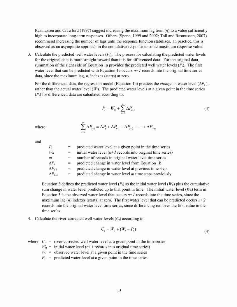
Equation 4 states that the corrected well water level at a given point in time (Ct) after the initial water level (W0) is the residual difference between the observed (Wt) and predicted (Pt) value at that point in time.

Figure 1.3 illustrates the observed, predicted, and corrected water level results for well 399-1-21A (located about 320 meters inland) when using the differenced data option and a maximum lag (n) of 480 hours.

Figure 1.3. Observed, Predicted, and Corrected Water Level Results for Well 399-1-21A

1.2.2 Multiple-Regression Models Issues

There are a number of assumptions and limitations related to multiple regression. Those that are more relevant and obvious are discussed briefly here. The reader is directed to statistical textbooks covering this topic (e.g., Pankratz, 1991) for a more in-depth and comprehensive discussion of multiple regression, its assumptions, and limitations. In multiple regression it is assumed that 1) the input (stress) variables are not perfectly auto correlated with each other and independent from the dependant (response) variable, 2) the regression residuals are normally distributed with a mean of zero, have constant variance, and are not auto correlated/collinear (Pankratz, 1991; Stevens, 1996). It is inevitable that river-stage and well water levels will lack complete independence, due to the open, hydraulically communicative exchange between surface and groundwater. It also expected that the time-lagged input river-stage data are going to have a degree of autocorrelation. Violation of these assumptions does not necessarily preclude the use of multiple regression for the application of river or barometric correction or invalidate the regression estimates (intercept and coefficients); however, it does call into question statistical hypothesis testing. The statistical parameters can be used diagnostically to guide end users in determining the optimum maximum time lag for prediction and correction applications, but they should not be used to signify statistical significance. The well-established conceptual and analytical basis for time-lagged river-stage effects, with responses often requiring extended period of time (e.g., days to months) to become fully manifested in distant, inland wells supports the use of multiple-regression convolution/deconvolution as valid method for identifying and removing their effects (Spane and

1.7

Mackley, 2010). However, caution needs to be exercised on the part of the analyst not to put too much confidence in the statistical metrics such as R2 or p-values when the above-mentioned assumptions are violated.

The goodness-of-fit metrics reported by MRCX include the R2, adjusted R2, and the MAE of the regression model. Of the three, the MAE is considered the least biased indicator of the goodness-of-fit, with lower values indicating improved model fit. All three serve as diagnostic indicators of the ability of the predictions from the regression model to fit the observed data, but none of them should be used to quantitatively test for statistical significance, due to the above-mentioned assumption violations.

Lastly, it should be reiterated that there may be other frequency-based or time-series techniques in addition to the established method of Rasmussen and Crawford (1997) that could also be used to predict river-stage effects on well water levels. ARIMA (Box et al., 2008) or distributed-lag transfer functions (Pankratz, 1991) might also be effective. Examining and comparing the efficacy of different forecasting techniques, although out of the scope of this task, is a worthwhile research objective.

2.1

2.0 Software Installation and Configuration

The Multiple Regression Correction in Excel (MRCX v.1.1) software tool is distributed as a single .MSI Windows Installer file (MRCX_v1.1.MSI). The .MSI installer program installs a collection of dynamic link library (.DLL) files that contain the compiled statistical and processing functions as well as the Excel 2007 macro-enabled workbook template (MRCX_v1.1.xlsm). The installation of the MRCX Windows Installer files is discussed below, followed by instructions for opening of the Excel macro-enabled workbook file.

2.1 Installing the MRCX v.1.1 Software Files

The first step is to install the .MSI Windows Installer file. This will install a collection of .dll files that perform the highly-computation portion of the multiple-regression and place a local copy of the MRCX Excel worksheet template file on your computer. The steps for installing MRCX with the .MSI Windows Installer file are:

1. Remove any previous versions of MRCX using the Add or Remove Programs within the Control Panel in Windows.

2. Exit out of Microsoft Excel prior to attempting the install.

3. Double-click on the MRCX_v1.1.MSI install file. This will bring up Setup Wizard.

4. Click on Next to proceed.

5. Select the installation folder path for the MRCX files.

6. Click on Next. This will bring up the confirmation screen.

7. Click on Next to finish the install.

8. When the program is successfully installed, click on Close to exit the Setup Wizard.

Although you do not need full administrator privileges on the computer you are installing MRCX on, some level of program installation permissions are needed.

2.2 File Saving and Renaming

The MRCX_v1.1.xlsm workbook contains a default data entry and model configuration template and Visual Basic for Applications (VBA) code for performing the river-correction process. Users are encouraged to re-save and rename the template as desired. However, you must save each renamed instance of the MRCX template workbook as an Excel 2007 macro-enabled workbook (.xlsm file format) or the full MRCX river-correction functionality will be lost.

The MRCX Excel software tool will be referred to by its original name (MRCX_v.1.1.xlsm) in this document for consistency. As noted above, you can resave the workbook under a different filename. The guidance and information content herein applies equally to renamed instances of the MRCX workbook as long as the structural contents of the original MRCX_v1.1.xlsm workbook template are retained. The filename does not affect the functionality of the MRCX VBA code.

2.2

2.3 Configuring the MRCX Workbook Template

The MRCX_v1.1.xlsm file will be installed into the user-selected folder during the installation described above. This file is an Excel 2007 macro-enabled workbook. It designed to enable the end user the functionality to perform the river correction process within a single software environment. It interacts with the library of .dll files using VBA.

2.3.1 Enabling the MRCX VBA Macro in Excel 2007

Since the Excel template workbook contains VBA code, it is considered a macro-enabled workbook and has the .xlsm file extension. The macro security settings in Excel may need to be adjusted in order to enable the VBA code in the MRCX_v1.1.xlsm file to function, depending upon the user’s current settings. Excel 2007 has the following Macro Security Setting Options:

1. Disable all macros without notification

2. Disable all macros with notification

3. Disable all macros except digitally signed macros

4. Enable all macros (not recommended; potentially dangerous code can run)

If the macro security is set to option 1, you will not be able run any type of macro. The other three macro security options allow macros to be enabled either on a case-by-case basis or permanently. Macro security option 2 disables macros from running initially unless the user manually enables the specific file – this is the temporary macro enable option described below. Option 3 restricts all macros except those containing digitally-signed certificates – this is not an option since the MRCX Excel workbook file is not digitally signed. Option 4 allows all macros to be enabled and is not recommended.

If you have your macro security settings configured to option 2 (Disable all macros with notification), Excel will initially disable the MRCX code from running when the workbook file is opened. It places a notification in the Excel toolbar Ribbon (Figure 2.1). For instructions on configuring your Excel 2007 macro security settings set to option 2 see the help file in Excel. Once you have set Excel to macro security option 2, you are ready to open the MRCX workbook file and enable temporary access to the MRCX VBA code. To enable temporary access to the VBA code in MRCX, follow the steps below each time you open the workbook:

1. Open the MRCX_v1.1.xlsm workbook file.

2. Click on the Options button on the Security Warning notification on the Excel toolbar ribbon (Figure 2.1)

3. Select the Enable this content option (Figure 2.2) to temporarily enable the MRCX VBA macro.

Figure 2.1. Macro Security Warning Notification on the Excel 2007 Toolbar Ribbon

2.3

Figure 2.2. Enabling Temporary Macro Permission

4. Click on OK to save and close the macro settings.

The Security Warning notification will no longer be visible on the Excel toolbar ribbon and the MRCX VBA macro should be enabled. You will need to follow the steps listed above every time you open a MRCX macro-enabled workbook.

3.1

3.0 User Interface

The MRCX Excel workbook template (MRCX_v1.1.xlsm) was designed as a software tool for a broad audience of end users to perform river correction of well water levels within a single user environment. It contains a collection of worksheets for input data, model configuration, and output results. There are drop-down lists and command buttons that allow the user to configure the multiple-regression convolution/deconvolution correction settings with flexibility.

As noted above, the original MRCX workbook file can be resaved under a different name as desired, with the imposed restriction that it is saved as an Excel 2007 macro-enabled workbook (.xlsm file format). This section introduces the general features and functionality of the MRCX workbook template components. Instructions for utilizing the features of the MRCX software tool then discussed in order of the river-correction process.

3.1 General Overview

The MRCX software tool is a single workbook template organized into four worksheets, organized by workflow process. These include Input Data, Model Config, Training Results, and Correction Results. They contain a mixture of locked and editable cells.

It is important to reiterate that the structural form (rows and columns) is directly tied to the functionality of the VBA code, particularly for the Input Data and Model Config worksheets. Changes to the structural form (e.g., inserting/deleting a column) will alter cell mapping between the worksheets and the VBA code, resulting in loss of functionality or erroneous results. The general workflow process for river correction in MRCX v.1.1 is depicted in Figure 3.1.

3.2

Figure 3.1. Generalized MRCX Workflow Process Diagram

The MRCX workbook can be viewed at any zoom level within Excel; however, the drop-down lists and graphs were sized to be viewed at about 85% zoom level on a 19-inch monitor configured to display at 1280 by 1024 dpi resolution. You may need to adjust the zoom level to your particular monitor screen size and resolution.

3.3

3.2 Input Data

The Input Data worksheet contains place holders for the data that will be used in the river-correction process (Figure 3.2). It is organized into Training and Correction ranges. The two time series of data are distinguished from each other in order to extend the flexibility and capability of the MRCX software tool. It is often desirable to “train” the multiple regression convolution/deconvolution model using one set of data, and then make river-level correction on another set of data. For example, you can use several months of water level data preceding a hydraulic test as the training data. The RRF generated from the training data can then be used to correct the data collected during a hydrologic test.

Figure 3.2. Input Data Worksheet

There are three command buttons embedded into the Input Data worksheet for convenience. The ‘Set Correction Data Equal to Training Data’ command button will copy the data from the training to the correction input range. The ‘Clear Training Data’ and ‘Clear Correction Data’ command buttons reset and clear the corresponding input data ranges in the worksheet.

3.2.1 Copy Paste Special-Values

The MRCX workbook template is designed for users to make changes to the values in the data input and model parameter cells as part of the workflow process (Figure 3.1); however, changes to the row and column structure and cell formulas will impact the functionality of MRCX.

3.4

It is essential that you use the Copy Paste Special-Values command in Excel when copying the training and correction data into the Data Input worksheet. This will ensure cell formatting remains intact. As noted above, changes to the structural format of the MRCX workbook will cause the program to either fail completely or produce erroneous results. This can easily be avoided by utilizing the Copy Paste Special-Values feature in Excel (refer to the help files in Excel if you are unfamiliar with using this feature).

3.2.2 Training Data

The input data in the Training Dataset range are used to “train” the multiple regression convolution/deconvolution model and generate a RRF that will be used to calculate predicted and corrected well water levels under the influence of river-stage effects. Entering the training data is the first step in the river-correction workflow process within MRCX (Figure 3.1). As mentioned before, these are the primary data used to create the RRF used to predict (convolution) and remove (deconvolution) river-stage effects.

3.2.3 Correction data

The MRCX interface allows users to enter different time-series of data in the Correction Dataset section of the Input Data worksheet. This feature was included to allow greater flexibility with training versus correction periods. The RRF is generated by the training data and can then be extended for use to the separate correction data. The primary difference between the training and correction data is that the correction data can and often do contain groundwater responses from sources other than the river (e.g., pumping test). The response of these non-river input stresses is often obscured in the water level data due to river-stage effects.

Unlike the training data, the correction data does not need be entered into the Input Data worksheet prior to generating the RRF function. It needs to be added prior to running the ‘Run Multiple Regression Model on Correction Data’ command button on the Model Config worksheet (discussed below).

3.2.4 Input Data Requirements

The river-correction method and the code in the MRCX assume the input data meet structural, formatting, and technical requirements. For the MRCX code to work properly, the following general format requirements for the training and correction data sets should be met:

1. Data must be continuous – that is, there are no data gaps or missing intervals of data

2. Data must be chronologically sequenced at a constant interval (e.g., entire time series is on hourly interval)

3. Date values need to be in MM/DD/YYYY HH:MM format (e.g., 01/01/2010 15:00)

4. River stage and well water levels need to be in a number format with values no more than ten decimal places (e.g., 115.215)

5. The number of records (rows) for each time series cannot exceed 32,000. (note: To clarify: this restriction is for each input data type – in other words, the training and correction data can each have 32,000 records i.e.,, rows)

3.5

Additionally, the training and correction data need to meet technical assumptions in order to generate effective and scientifically defensible river correction:

1. Have similar well hydrologic conditions between the training and correction data (e.g., saturated aquifer thickness, magnitude and frequency of river-stage changes)

2. Collected in a similar manner (e.g., consistent source of water level data)

3. Training data contain or is of a sufficient time period to adequately capture associated, long-term river-stage responses influence.

4. The maximum lag value must be less than 0.5 times the number of input data records minus two time units. For example, if the input data contains 1,000 hourly-spaced records. The maximum lag value must not exceed 498 hours. This is a technical requirement imposed by the multiple regression function specifically used by MRCX in order to reach a solution for the model estimates.

3.3 Model Configuration

The Model Config worksheet contains the main user interface for MRCX (Figure 3.3). It contains a pre-generated collection of drop-down lists, input cells, command buttons, and diagnostic plots for setting model parameters and running the multiple regression deconvolution/convolution method for river correction. Note: users can add/modify the existing plots (e.g. scale on axes). Unlike the Input Data worksheet, no copying or pasting of data values is necessary in the Model Config worksheet. However, similar to the other MRCX worksheets, changing the structural format of the worksheet will prevent the VBA code from running properly (e.g., inserting/deleting rows or columns).

Figure 3.3. Model Config Worksheet

3.6

The use of the model configuration features and command buttons will be discussed below in the context of the river-correction workflow process outlined in Figure 3.1. Additional application of these features is contained in the Tutorial Example section.

3.3.1 Time Filtering

It may be desirable to focus on a particular time period of the input data during model training and correction (Figure 3.4). Typically, the training period should consist of a time when well water-level responses are known to be solely responding to river-stage fluctuations and not subjected to other interfering extraneous effects (e.g., pumping activities). The available time range (start and end data/time) is displayed. The input data for both the training and the correction data can be filtered to a customized time range by entering a filter start and end date. The start and end dates must fall within the available time range or an error message will be displayed.

The Reset Filter command buttons above the training and correction time filter options will reset the start and end date/time to the minimum and maximum available values available, respectively. Note: remember to reset the time filtering options each time you copy new data to the Input Data worksheet – they do not automatically reset.

Keep in mind, that you need to set the start date n or n+1 time units previously to the date/time you want the output from the regression model to begin, when using the Original Data and First Differences data options, respectively (where n is the maximum time lag). For example, if you want the river correction results to start on 05/01/2010 0:00 using the Differenced Data option and a maximum lag (n) of 480 hours, you would set the start date to 04/10/2010 23:00 (482 hours previously).

Figure 3.4. Time Filtering Settings

3.3.2 Data Value Option

MRCX give users the option to run the multiple model using either the original data or first differences of the original data (i.e., changes in river stage and well water level between successive time periods). Rasmussen and Crawford (1997) reported better success with using original data in the regression deconvolution correction of barometric effects. However, others have chosen to use the first differences instead for barometric (Spane 1999 and 2002; Toll and Rasmussen 2007) and river correction (Vermeul et al., 2009; Spane and Mackley, 2010).

Differencing is a common transformation technique used in time-series analysis to minimize systematic changes in the mean (trend) and create a more stationary (constant mean and variance) data set (Pankratz, 1991). One of the advantages to running the model on the first differences is that this method is consistent with the concept that it is the changes in river stage and not the actual river-stage elevations themselves that creates the time-lagged and attenuated well water level responses.

3.7

The inherent correlation of river-stage and well water elevations might cause the OLS regression model to be less stable when using the original data. However, this has not been fully evaluated by the authors. An advantage of using the original data in the regression is that you can achieve a “rough” prediction and correction using fewer lags, although the response function is less stable and the overall goodness-of-fit is typically lower. Fewer lags means that the training period can be shorter since the training period must have slightly more than two times the number of records as the lag term in order for the regression model to run properly. Both methods may have application depending upon the existing well/aquifer/river communicative conditions. Further evaluation and comparison of the two methods beyond the scope of the development of this software tool is needed to better understand the relative effectiveness of one method over the other. MRCX allows both data options as a means of providing a higher degree of model functionality.

To select the data option, click inside the Data Option cell and select one of the two options from the drop-down list (Figure 3.5).

Figure 3.5. Data Value Type Option Configuration Setting

3.3.3 Lag Option

MRCX allows two different lag options for running multiple regression on the specified training data set, Manual and Batch mode. In Manual lag mode, the regression model is run for a single, specified, maximum time -lag value. This is the default mode in MRCX. Alternatively, in Batch lag mode, users can create a list of maximum lag values, and a separate regression model will be run for each lag. In the Batch mode, model results are saved in a separate Excel workbook, with results for each regression model run saved in individual worksheets. The Batch lag option was included in MRCX to allow users to compare regression results for the same training data for varying maximum time-lag values.

3.8

MRCX may require up to several minutes to process results for a single multiple-regression model for large data sets and lag values. Processing times will also vary as a function of performance capabilities of the individual computer system running MRCX code. The Batch mode option also allows users to process a large batch of regression training models for various maximum lag values and outputs the regression results into a single external Excel workbook file. This may be preferable to individually changing the maximum time-lag value and comparing regression results in a trial-and-error fashion using the Manual option within the Model Config worksheet.

To select the lag option, click inside the Lag Option cell and select one of the two options from the drop-down list (Figure 3.6).

Figure 3.6. Lag Option Configuration Setting

3.3.4 Maximum Number of Lags

The maximum number of time lags (n) to be used in the multiple regression model is specified by entering a value into the Lags input box (Figure 3.7). Maximum lag values are restricted to a single integer value between 0 and 10,000. The lag units are the same as the interval units for the records in the input data. For example, if the training and correction data consist of hourly river-stage and water level measurements, units for the lags will be hours.

As discussed in Section 1.2.1, the maximum number of lags should be increased until either the RRF asymptotically approaches a maximum cumulative response value or there is no major improvement in the model results (Rasmussen and Crawford, 1997; Toll and Rasmussen, 2007; Spane and Mackley, 2010). In practice, maximum lags of several hundred hours or more may be necessary to adequately capture the full river-stage effects in water levels in wells located several hundred meters from the river (e.g., Vermeul et al., 2008; Spane and Mackley, 2010).

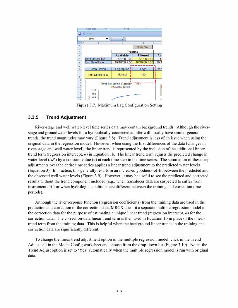
3.9

Figure 3.7. Maximum Lag Configuration Setting

3.3.5 Trend Adjustment

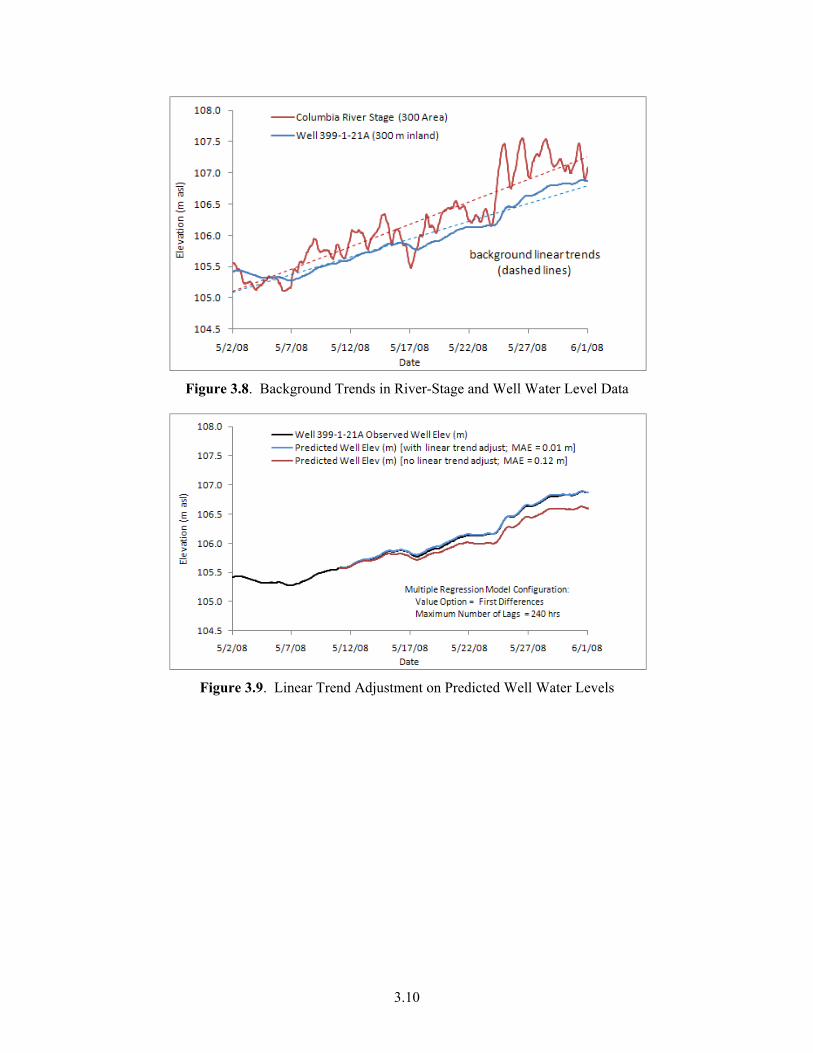
River-stage and well water-level time series data may contain background trends. Although the river-stage and groundwater levels for a hydraulically-connected aquifer will usually have similar general trends, the trend magnitudes may vary (Figure 3.8). Trend adjustment is less of an issue when using the original data in the regression model. However, when using the first differences of the data (changes in river-stage and well water level), the linear trend is represented by the inclusion of the additional linear trend term (regression intercept, α) in Equation 1b. The linear trend term adjusts the predicted change in water level (∆Pt) by a constant value (α) at each time step in the time series. The summation of these step adjustments over the entire time series applies a linear trend adjustment to the predicted water levels (Equation 3). In practice, this generally results in an increased goodness-of-fit between the predicted and the observed well water levels (Figure 3.9). However, it may be useful to see the predicted and corrected results without the trend component included (e.g., when transducer data are suspected to suffer from instrument drift or when hydrologic conditions are different between the training and correction time periods).

Although the river response function (regression coefficients) from the training data are used in the prediction and correction of the correction data, MRCX does fit a separate multiple regression model to the correction data for the purpose of estimating a unique linear trend (regression intercept, α) for the correction data. The correction-data linear trend term is then used in Equation 1b in place of the linear-trend term from the training data. This is helpful when the background linear trends in the training and correction data are significantly different.

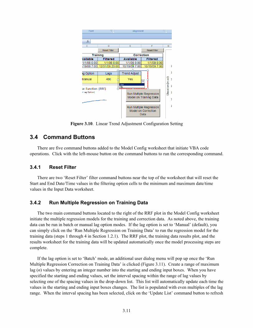
To change the linear trend adjustment option in the multiple regression model, click in the Trend Adjust cell in the Model Config worksheet and choose from the drop-down list (Figure 3.10). Note: the Trend Adjust option is set to ‘Yes’ automatically when the multiple regression model is run with original data.

3.10

Figure 3.8. Background Trends in River-Stage and Well Water Level Data

Figure 3.9. Linear Trend Adjustment on Predicted Well Water Levels

3.11

Figure 3.10. Linear Trend Adjustment Configuration Setting

3.4 Command Buttons

There are five command buttons added to the Model Config worksheet that initiate VBA code operations. Click with the left-mouse button on the command buttons to run the corresponding command.

3.4.1 Reset Filter

There are two ‘Reset Filter’ filter command buttons near the top of the worksheet that will reset the Start and End Date/Time values in the filtering option cells to the minimum and maximum date/time values in the Input Data worksheet.

3.4.2 Run Multiple Regression on Training Data

The two main command buttons located to the right of the RRF plot in the Model Config worksheet initiate the multiple regression models for the training and correction data. As noted above, the training data can be run in batch or manual lag option modes. If the lag option is set to ‘Manual’ (default), you can simply click on the ‘Run Multiple Regression on Training Data’ to run the regression model for the training data (steps 1 through 4 in Section 1.2.1). The RRF plot, the training data results plot, and the results worksheet for the training data will be updated automatically once the model processing steps are complete.

If the lag option is set to ‘Batch’ mode, an additional user dialog menu will pop up once the ‘Run Multiple Regression Correction on Training Data’ is clicked (Figure 3.11). Create a range of maximum lag (n) values by entering an integer number into the starting and ending input boxes. When you have specified the starting and ending values, set the interval spacing within the range of lag values by selecting one of the spacing values in the drop-down list. This list will automatically update each time the values in the starting and ending input boxes changes. The list is populated with even multiples of the lag range. When the interval spacing has been selected, click on the ‘Update List’ command button to refresh

3.12

the list in the frame on the right side of the menu. Users have the option to output the predicted and corrected results in addition to the summary results by check the option box in the dialog box. Click on the ‘Run Model’ command button to begin the multiple regression for the batch of maximum lags listed. In batch mode, the results will be saved in a new external Excel workbook file. The workbook file contains a summary worksheet and separate worksheets for each maximum lag value in the batch list. Be patient while the batch of regression models is processed – this can take several minutes or longer. The Windows “hour glass” cursor will show while the batch regression is processing. When it is complete, a message box will appear with “Finished Running Batch-Mode Multiple Regression on Training Data.”

It is also possible that your computer will run out of memory and return and error if your batch list is long, the number of records in the input data is large, the maximum lag values are large, and/or you have limited memory resources available on your computer. If this happens, the easiest solution is to decrease the number of maximum lag values in the batch list – in other words, split up your batch list into multiple batches then run them separately.

Figure 3.11. Batch (Multiple) Lag Option Dialog Menu

Once the RRF has been generated from the training data, you can click the ‘Run Multiple Regression Model on Correction Data’ command button to run the regression model on the correction data. The correction data results plot and the correction results worksheets will then be automatically updated. Note: the batch maximum lag option is not available for the correction data regression model.

3.5 Results

The results from the multiple regression model are displayed in plots within the Model Config worksheet and stored in worksheets within the MRCX workbook. The observed, predicted, and corrected well water levels for the training and correction data are shown in separate plots in the Model Config worksheet. The RRF generated from the training data is also included for diagnostic purposes. Users are free to customize the plot properties within the Model Config worksheet.

The model results for the training and correction data are automatically output to the corresponding result worksheets in the MRCX workbook. You can quickly clear the results by clicking on the ‘Clear All Results’ command button on the Model Config worksheet.

3.13

The individual and cumulative regression coefficients (βi’s) for each lag (0 to n) from the multiple regression model are included in the results worksheets. The MRCX code is designed to utilize the regression coefficients from the respective training results worksheet when processing the predicted and corrected water levels for the correction data.

Goodness-of-fit statistics and model configuration settings are also included in the model summary section of the results worksheet. The R2, adjusted R2, and the MAE provide an indication on the ability of the multiple regression model to explain well water levels with time-lagged input from the river. As previously discussed, they should be used as diagnostic indicators and not as quantitative metrics for establishing statistical significance due to non-standard model conditions (e.g., stationarity, collinearity, autocorrelation, etc.).

The results worksheet also contains the river stage, observed, predicted, and corrected well water level time series. Note: the predicted and corrected water levels contain a large number of decimal places. These do not reflect the precision of the model. Keep in mind the goodness-of-fit statistics from the model when interpreting these values and round them to appropriate significant figures.

4.1

4.0 Tutorial Examples

This section includes examples of the multiple regression technique from two different Hanford Site field settings. It is written in tutorial form for users to follow step-by-step instructions. It assumes that the user has already successfully installed MRCX v.1.1 onto their local computer and has opened the MRCX workbook in Excel. See Section 2.1 above for instruction on installing MRCX.

The first Hanford Site example is for a test well (399-1-21A) completed in the Hanford formation and exhibits excellent hydraulic communication and high aquifer diffusivity. River-stage effects for this well are easily identified and removed. In contrast, the second Hanford Site example is for a well completed in the lower permeability Ringold Formation and is in close proximity to extraction wells used within the 100-K Area pump-and-treat system. This example demonstrates the difficulties in removing river-stage effects from well response records which may be significantly impacted by extraneous stress effects (i.e., surrounding pumping). The difficulty centers on finding a baseline well record not adversely impacted by extraneous stress effects so that a representative data record can be used as part of the MRCX training analysis for developing an associated river response function. The motivation for including a problematic data set such as this is that end users are likely to encounter similar challenges and need to be aware of the complications associated with such “noisy” data sets and the limitations for removing river-stage effects in wells such as this one.

4.1 Example 1: Well 399-1-21A

The first tutorial example involves removal of river-stage effects for well 399-1-21A, in the 300 Area of the Hanford Site. It is located about 323 meters from the river and is completed in the permeable Hanford formation (Figure 4.1). It provides an excellent example of a well with a highly associated river response behavior (RRF ≥ 0.8), sufficient to allow for good river correction of well water levels. Spane and Mackley (2010) used this well as a demonstration example of the multiple-regression correction methodology. The following steps will guide you through the process of correcting river-stage effects for this well and highlight some of the different MRCX user options.

Figure 4.1. Site Map of 300 Area Wells

4.2

4.1.1 Entering the Input Data

The first step is to enter the river-stage and well water level data into the MRCX workbook. The time-series data for the 300-Area river gage and well 399-1-21A is located in the \Tutorial subfolder in the MRCX folder created during the initial installation of MRCX.

Open the 300_Area_Example_InputData.xlsx workbook file from the C:\MRCX\Tutorial\ subfolder. This workbook contains the hourly river gage and well data.

Select the entire three-column data range (excluding the header).

Select Copy (Ctrl + C) from the Excel Home Ribbon tab.

Switch back to the MRCX workbook file.

Click on cell B4 in the Input Data worksheet to set this as the destination location for the next step.

Select Paste > Paste Values from the Excel Home Ribbon tab (Figure 4.2). This will paste the input values into the three Training Dataset columns. The Training Data time-series plot now be updated, showing river and well elevations.

Figure 4.2. Paste Values Option in Excel

Click on the ‘Set Correction Data Equal to Training Data’ command button above the time-series plots in the Input Config worksheet. This will copy the data in the Training Dataset section into the Correction Dataset section. The plots for the training and correction data should be similar in appearance (Figure 4.3).

4.3

Figure 4.3. Well 399-1-21A Input Data Worksheet

4.1.2 Configuring the Multiple Regression Model

Activate the Model Config worksheet.

Click on the ‘Reset Filter’ command buttons, located at the top of the Model Config worksheet, for both the training and correction time periods. It is important to reset the time filters each time you enter new data into the Input Data worksheet. This will ensure the filter start/end dates are within the valid date range of the input data.

Leave the filter start date default of 1/1/08 0:00 for the training data (cell D5).

Set the filter end date for the training data to 12/31/08 23:00 (cell D6). This will restrict the training range to only use data from 2008.

Set the filter start date for the correction data to 1/1/09 0:00 (cell F5).

Leave the filter end date default of 10/19/09 7:00 for the correction data (cell F6) (Figure 4.4).

Figure 4.4. 399-1-21A Config Options

4.4

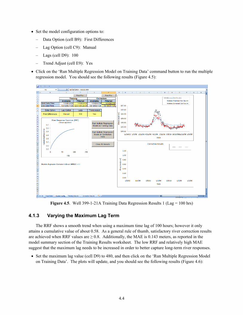
Set the model configuration options to:

– Data Option (cell B9): First Differences

– Lag Option (cell C9): Manual

– Lags (cell D9): 100

– Trend Adjust (cell E9): Yes

Click on the ‘Run Multiple Regression Model on Training Data’ command button to run the multiple regression model. You should see the following results (Figure 4.5):

Figure 4.5. Well 399-1-21A Training Data Regression Results 1 (Lag = 100 hrs)

4.1.3 Varying the Maximum Lag Term

The RRF shows a smooth trend when using a maximum time lag of 100 hours; however it only attains a cumulative value of about 0.58. As a general rule of thumb, satisfactory river correction results are achieved when RRF values are ≥ 0.8. Additionally, the MAE is 0.143 meters, as reported in the model summary section of the Training Results worksheet. The low RRF and relatively high MAE suggest that the maximum lag needs to be increased in order to better capture long-term river responses.

Set the maximum lag value (cell D9) to 480, and then click on the ‘Run Multiple Regression Model on Training Data’. The plots will update, and you should see the following results (Figure 4.6):

4.5

Figure 4.6. Well 399-1-21A Training Data Regression Results 2 (Lag = 480 hrs)

The increase of the lag to 480 hours results in a much improved match between the predicted and the corrected data. The RRF approaches a maximum value of 0.88, and the MAE equals 0.031 meters. This suggests a valid model fitting for the training data, consisting of the data for the entire year of 2008. The model does show under-prediction in the well water levels during the high river-stage period of 2008. There may be a storage effect of the water table increasing on a seasonal time scale that is not fully captured in the average river response function with a maximum time lag of 480 hours.

4.1.4 Different Training and Correction Time Periods

Often, it is will be desirable to focus on a particular time period for the correction rather than for the entire data set. In the next step, the objective is to correct river effects during the first four months of 2009. You can use data from the same time period to train the model; however, a more robust application of the correction method is to train the model with data from a different time period than will be corrected. To be representative, the training period should have similar river-stage, well water elevation relationship, and hydrologic conditions as the correction time period. In the next step, data from the first four months of 2008 will be used to train the model and develop the RRF for correction for the first four months of 2009.

Verify the model configuration options are still set to:





4.6

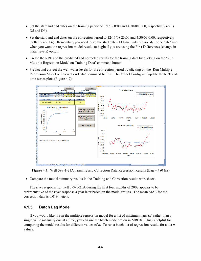
Set the start and end dates on the training period to 1/1/08 0:00 and 4/30/08 0:00, respectively (cells D5 and D6).

Set the start and end dates on the correction period to 12/11/08 23:00 and 4/30/09 0:00, respectively (cells F5 and F6). Remember, you need to set the start date n+1 time units previously to the date/time when you want the regression model results to begin if you are using the First Differences (change in water levels) option.

Create the RRF and the predicted and corrected results for the training data by clicking on the ‘Run Multiple Regression Model on Training Data’ command button.

Predict and correct the well water levels for the correction period by clicking on the ‘Run Multiple Regression Model on Correction Data’ command button. The Model Config will update the RRF and time-series plots (Figure 4.7):

Figure 4.7. Well 399-1-21A Training and Correction Data Regression Results (Lag = 480 hrs)

Compare the model summary results in the Training and Correction results worksheets.

The river response for well 399-1-21A during the first four months of 2008 appears to be representative of the river response a year later based on the model results. The mean MAE for the correction data is 0.019 meters.

4.1.5 Batch Lag Mode

If you would like to run the multiple regression model for a list of maximum lags (n) rather than a single value manually one at a time, you can use the batch mode option in MRCX. This is helpful for comparing the model results for different values of n. To run a batch list of regression results for a list n values:

4.7

Set the Lag Option (cell C9) to Batch using the drop-down list prior to running the regression model for the training data. This will bring up a dialog box containing additional user input options (Figure 4.8).

Figure 4.8. Batch Lag Menu

Set the Starting and Ending values for the range of maximum lag values to 0 and 500, respectively.

Select one of the Interval Spacing items in the drop-down list.

Click on the ‘Update List’ command button to display the list of maximum lag values that will be run in batch mode.

Click in the box next to the ‘Output Predicted and Corrected Values’ to include the full results in the output workbook. Disabling this option will output just the summary results for the batch correction.

Click on the ‘Run Model’ command button to initiate the batch mode. Note: if the list is long and the maximum lag values are large, the batch regression results can take several minutes to process. When complete, a message box will appear letting you know the processing is complete (Figure 4.9).

Figure 4.9. Batch Lag Menu

In batch mode, MRCX creates a new workbook file containing individual worksheets for each item in the batch list of maximum lag values. The result worksheets are named according to the corresponding lag value.

Click on the ‘Summary’ worksheet to view a table showing a summary of the regression results for each of the values in the maximum lag list.

Click on each worksheet to compare the results for varying maximum lag values.

4.2 Example 2: Well 199-K-112A

This example will involve using various regression options in MRCX while correcting water level data for well 199-K-112A. As noted above, this well was chosen to highlight the challenges and

4.8

limitations of river-stage correction when dealing with a complicated data set that includes extraneous influences such as nearby pumping wells.

Well 199-K-112A is located 115 meters inland from the river shoreline in the 100-K area of the Hanford Site and is screened in the Ringold Formation (Figure 4.10). The Ringold Formation has a relatively lower permeability than the Hanford formation, so the river response might be expected to be more lagged and attenuated than the response observed in the first example for well 399-1-21A. On the other hand, well 199-K-112A is almost three times closer to the river than well 399-1-21A (323 m inland). The river response function would need to be normalized for inland distance to make direct comparisons between wells – this involves plotting RRF’s against the distance-normalized time lag where (time lag divided by the square of the inland distance). We will not do that in this exercise, but you might want to explore the comparison on your own.

Figure 4.10. Site Map of 100-K Wells

Well 199-K-112A is located 5 meters away from the pump-and-treat extraction well 199-K-129 (also screened in the Ringold Formation) and within a few hundred meters of several other extraction wells. During the 2008 and 2009 time period of interest, well 199-K-129 was mostly running, but experienced intermittent shut-down events. These shut-down events created recovery responses in well 199-K-112A. However, river-stage effects make these recovery responses less obvious and obscure their overall magnitude. This example will illustrate the difficulty in correcting river-stage effects with data that contain non-river input signals.

4.9

4.2.1 Input Data

The time-series data for the 100-K river gage and well 199-K-112A is located in \Tutorial subfolder in the MRCX folder created during the initial installation of MRCX.

Open the 100K_Area_Example_InputData.xlsx workbook file. This workbook contains the hourly river gage and well data in a worksheet named ‘Elev Data’. It also contains pumping flow rate data for the adjacent extraction well in a worksheet named ‘Flow Data’.

Open a new instance of the MRCX workbook template, and clear the results and the input data using the command buttons in MRCX if needed.

Follow the steps outlined in Section 1.1.1 for copying the river-stage and well water level from the source workbook to the target cells in the Input Data worksheet in the MRCX workbook file.

Use the ‘Set Correction Data Equal to Training Data’ command button in the Input Data worksheet to copy the data from the training section to the correction sections.

You are now ready to configure the multiple regression model settings in the Model Config worksheet.

4.2.2 Establishing a Suitable Training Period and Maximum Lag Combination

As noted above, the presence of the intermittent pumping of the adjacent extraction well creates additional complexity to the correction process (Figure 4.11). In the following steps, we will attempt to look for a suitable training period that can be used to generate a river response function to correct a select period of time in 2009 when a major shut down even occurred (04/29/08 to 05/17/09). River-stage effects obscure the recovery response to the extraction well shut down. The objective is to remove or minimize river-stage effects in order to better evaluate the recovery response.

Figure 4.11. Average Daily Pumping Rates Data for Extraction Well 199-K-129

Typically, the ideal scenario would be to train the response function during a period when the extraction well has been shut down for an extended period of time. Unfortunately, the longest shut down

4.10

period is only about 40 days (06/5/08 to 07/14/08), which is too short of a time period to adequately incorporate longer-term (e.g., seasonal) river-stage influences. This will become apparent in the results generated in the next steps. To begin:

Activate the Model Config worksheet, and verify the following options:





Set the time filter options to:

– Training start date: 6/5/08 0:00

– Training end date: 7/14/08 0:00

– Correction end date: 4/1/09 0:00

– Correction start date: 6/15/09 0:00

Run the multiple regression model on the training data period to generate the RRF.

Run the multiple regression model on the correction data period.

Figure 4.12. Well 199-K-112A Regression Results 1 (Lag = 150 hours)

The river response function has a typical shape; however, it only reaches a maximum response of about 0.4 (Figure 4.12). This indicates either the well has a relatively weak river-stage effect or the maximum lag needs to be increased in order to incorporate longer-time scale river effects. Furthermore, the recovery response in April-May 2009 still contains noticeable river effects.

4.11

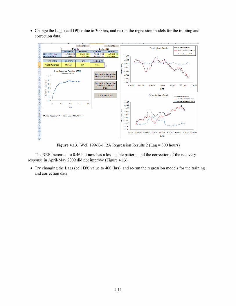
Change the Lags (cell D9) value to 300 hrs, and re-run the regression models for the training and correction data.


The RRF increased to 0.46 but now has a less-stable pattern, and the correction of the recovery response in April-May 2009 did not improve (Figure 4.13).

Try changing the Lags (cell D9) value to 400 (hrs), and re-run the regression models for the training and correction data.

4.12


Although there is a very strong match of the predicted and the observed water levels for the training period, the correction of the recovery response is worse than it was when using 150 or 300 hours for the lag Figure 4.14). Increasing the maximum lag to 400 hours resulted in a very unstable and non-characteristic pattern in the river response function. It suggests that the maximum lag term is too large for the short training period.

A different approach is to train the model on the entire 2008 and 2009 data set, lumping river and non-river influences in the response function. The advantage to this is that the longer training period can incorporate any longer-term river-stage effects that were absent in the 40-day training period. However, the obvious drawback to this approach is that the response function will contain non-river effects such as the intermittent pumping of well 199-K-129. Normally, this approach would be avoided. However, in the next step we will use all of the available data to train the RRF, and use it for correcting the April-May 2009 shut down recovery response. The caveat is that the river response function will be highly skewed by the extraneous (non-river) influences and should be interpreted with caution. To proceed:

Verify the model configuration options are still set to the following:





Click the ‘Reset Filter’ command button for the training data in order to set the options to:

– Training start date: 1/1/08 0:00

– Training end date: 7/1/09 0:00

4.13

Verify the correction start and end times are still set to the following:

– Correction end date: 4/1/09

– Correction start date: 6/15/19

Re-run the regression models for the training and correction data to generate new results.


The RRF increased to a higher value of 0.61 and the correction of the 2009 data improved (Figure 4.15). Although the RRF is still relatively low (indicating a relatively weaker river influence), and there are still residual river-stage effects present in the corrected data for April-May 2009, the recovery response pattern does have a more characteristic pattern. The apparent drop in the observed water levels around 5/6/09, due to a river-stage decrease, is now almost entirely removed.

4.2.3 Linear Trend Adjustment

MRCX allows the option to include or omit a background linear trend coefficient in the regression model. Thus far, we have included the background trend in all the regression models. To see the effect of leaving out the linear trend adjustment on the previous results:

Change the Linear Adjustment option (cell E9) to No by clicking in drop-down list.

Re-run the training and correction regression models.

The result of leaving out the background trend adjustment in the model is that the predicted values progressively deviate from the observed water levels with time (Figure 4.16). The corrected data for the 2009 recovery response has a slightly more positive trend compared to the previous results that included the trend adjustment. Although, the difference is small in this instance it may be more significant in other situations. The use of the trend adjustment option is highly dependent upon the situation – it is

4.14

recommended that you typically run the model with and without the trend adjustment and compare the results, especially when there is a very noticeable background trend in the observed well water level data.

Figure 4.16. Well 199-K-112A Regression Results with Linear Trend Adjust Turned Off

5.1

5.0 References

Barlow PM and AF Moench. 1998. “Analytical solutions and computer programs for hydraulic interaction of stream-aquifer systems.” U.S. Geological Survey, Open-File Report 98-415A, 85 p. Erskine AD. 1991. “The effect of tidal fluctuation on a coastal aquifer in the UK.” Ground Water, vol. 29, no. 4, pp. 556–562.

Box GEP, GM Jenkins, GC Reinsel. 2008. Time Series Analysis (4th Edition). John Wiley, New York.

Ferris JG. 1952. “Cyclic fluctuations of water level as a basis for determining aquifer transmissibility.” U.S. Geological Survey, Ground-Water Hydraulics Section, Contribution No. 1, 17 p.

Ferris JG. 1963. “Cyclic fluctuations of water level as a basis for determining aquifer transmissibility.” Water-Supply Paper 1536-I, U.S. Geological Survey, pp. 305–318.

Foundastat .Net Statistics Made Easy. 2008. FoundaStat Pro. Accessed (09/15/2010) at http://www.foundasoft.com/ (last updated 2008).

Furbish DJ. 1991. “The response of water level in a well to a time series of atmospheric loading under confined conditions.” Water Resources Research, vol. 27, no. 4, pp. 557–568.

Gilmore TJ, FA Spane, Jr., DR Newcomer, and CR Sherwood. 1992. Applications of three aquifer test methods for estimating hydraulic properties within the 100-N Area.” Pacific Northwest Laboratory, Richland, Washington.

Jacob CE. 1950. “Flow of groundwater.” In Engineering Hydraulics, H. Rouse (ed.), John Wiley & Sons, Inc., New York, pp. 321–386.

McDonald JP. 2007. Water-level barometric response analysis for the Liquid Effluent Retention Facility monitoring wells. SGW-35756, Rev. 0. Fluor Hanford, Inc., Richland, Washington

Pankratz A. 1983. Forecasting with univariate Box-Jenkins models: concepts and cases. John Wiley & Sons, New York.

Pankratz A. 1991. Forecasting with dynamic regression models. John Wiley, New York.

Rasmussen TC and LA Crawford. 1997. “Identifying and removing barometric pressure effects in confined and unconfined aquifers.” Ground Water, vol. 35, no. 3, pp. 502–511.

Spane FA, Jr. 1999. Effects of barometric fluctuations on well water-level measurements and aquifer test data. PNNL-13078, Pacific Northwest National Laboratory, Richland, Washington.

Spane FA. 2002. “Considering barometric pressure in groundwater flow investigations.” Water Resources Research, vol. 38, no. 6, pp. 14:1-18.

Spane FA, and RD Mackley. 2010. "Removal of River-Stage Fluctuations from Well Response Using Multiple-Regression." Ground Water in press.

5.2

Stevens J. 1996. Applied Multivariate Statistics for the Social Sciences (3rd Edition). Lawrence Erlbaum Associates, Inc., New Jersey.

Toll NJ and TC Rasmussen. 2007. “Removal of barometric pressure effects and earth tides from observed water levels.” Ground Water, vol. 45, no. 1, pp. 101–105.

Vermeul VR, BN Bjornstad, BG Fritz, JS Fruchter, RD Mackley, DR Newcomer, DP Mendoza, ML Rockhold, DM Wellman, and MD Williams. 2009. 300 Area uranium stabilization through polyphosphate injection: final report. PNNL-18529, Pacific Northwest National Laboratory, Richland, Washington.

Zlotnik VA and H. Huang. 1999. “Effect of shallow penetration and streambed sediments on aquifer response to stream stage fluctuations (analytical model).” Ground Water, vo. 37, no. 4, pp. 599–605.

PNNL 19775, Rev. 1

Distribution

No. of Copies

Distr.1

OFFSITE 2 S.S. Papadopulos & Assoc., Inc

7944 Wisconsin Ave. Bethesda, MD 20814 Matt Tonkin Rachel Shannon

ONSITE 12 CH2M-HILL Plateau Remediation

Company, Inc D.J. Alexander R3-60 R.S. Edrington R3-50 D. Erb R3-60 E.J. Freeman R3-50

M.J. Hartman R3-50 K.J. Johnson R3-50 J.P. McDonald R3-50

S.W. Petersen (3) R3-50 J.L. Smoot R3-50 L.C. Swanson R3-50

16 Pacific Northwest National Laboratory C.H. Allwardt K7-28 K.C. Carroll K6-96 M.D. Freshley K9-33 T.J. Gilmore K6-96 R.D. Mackley (5) K6-96 R.E. Peterson K6-75 T.C. Pulsipher K7-20 F.A. Spane K6-96 V.R. Vermeul K6-96 D.R. Newcomer K6-96 P.D. Thorne K6-96 M.D. Williams K6-96

guide to using multiple regression in excel (mrcx v.1.1) for · pdf file ·...

Documents