guidelines for project-level traffic forecasting hawaii · pdf filehawaii department of...
TRANSCRIPT

Guidelines for Project-Level Traffic Forecasting Hawaii Department of Transportation
Principal Investigators: Panos D. Prevedouros, PhD
University of Hawaii at Manoa and
Alan J. Horowitz, PhD University of Wisconsin, Milwaukee
with
Lambros Mitropoulos, PhD Alyx Yu, PhD
Liang Shi, PhD Candidate Daniel Lee, MSCE Candidate
Prepared for:
Hawaii Department of Transportation Prepared by:
University of Wisconsin – Milwaukee University of Hawaii at Manoa
Prepared in Cooperation with: State of Hawaii, Department of Transportation, Highways Division
and U.S. Department of Transportation, Federal Highway Administration
Honolulu, Hawaii
December 2015

ii
THE CONTENTS OF THIS REPORT REFLECT THE VIEWS OF THE AUTHORS, WHO ARE RESPONSIBLE FOR THE FACTS AND ACCURACY OF THE DATA PRESENTED HEREIN. THE CONTENTS DO NOT NECESSARILY REFLECT THE OFFICIAL VIEWS OR POLICIES OF THE STATE OF HAWAII, DEPARTMENT OF TRANSPORTATION OR THE FEDERAL HIGHWAY ADMINISTRATION. THIS REPORT DOES NOT CONSTITUTE A STANDARD, SPECIFICATION OR REGULATION.

iii
Table of Contents 1 Introduction ...............................................................................................................................1
1.1 Purpose ......................................................................................................................................... 1 1.1.1 Elements of a Forecast .......................................................................................................... 2 1.1.2 Project Types ......................................................................................................................... 2 1.1.3 Defining Forecast Requirements ........................................................................................... 3
1.2 Forecasting Process ....................................................................................................................... 6 1.2.1 Requesting a Forecast ........................................................................................................... 6 1.2.2 Forecasting Process Flow Diagram ....................................................................................... 1
1.3 Relationships consultants and other agencies.............................................................................. 2 1.4 National Guidelines ....................................................................................................................... 2 1.5 Choice of Techniques .................................................................................................................... 2 1.6 Quality Assurance and Validation Standards ................................................................................ 4
1.6.1 Inputs from Regional Model ................................................................................................. 4 1.6.2 Refined Outputs .................................................................................................................... 5
1.7 Errors and Variability in Volume Data ........................................................................................... 5 1.8 Half-Lane Rule and Extensions ...................................................................................................... 5 1.9 Limited Role of Judgment ............................................................................................................. 7
1.9.1 Appropriateness of Judgment ............................................................................................... 7 1.9.2 Asserting Parameter Values .................................................................................................. 7
1.10 Scenario/Sensitivity Testing .......................................................................................................... 7 1.11 Reporting of Reasonable Bounds on Forecast Values .................................................................. 8
1.11.1 Assessing Uncertainty ........................................................................................................... 8 1.11.2 Measures of Effectiveness (MOEs) ....................................................................................... 8
1.12 Documentation Standards ............................................................................................................ 8
2 Time Series Methods ..................................................................................................................9 2.1 Linear Regression Techniques ....................................................................................................... 9
2.1.1 Trend Models ........................................................................................................................ 9 2.1.2 Linear Models with Explanatory Variables.......................................................................... 11 2.1.3 Smoothing ........................................................................................................................... 14
2.2 Box-Jenkins/ARIMA Methods ..................................................................................................... 15 2.2.1 Autoregressive (AR) Models ............................................................................................... 15 2.2.2 Autoregressive with Explanatory Variables (ARX or SAR) Models ...................................... 17 2.2.3 Box-Cox Transformations .................................................................................................... 18
2.3 Time Series Examples .................................................................................................................. 20 2.3.1 Example 1: 2-Lane Rural Highway Site (Island of Maui) ..................................................... 20 2.3.2 Example 2: 6-Lane Freeway Site (Island of Oahu) ............................................................... 22 2.3.3 Example 3: An Autoregression Model with Box-Cox Transformation ............................... 24
2.4 Special Reporting Requirements ................................................................................................. 29
3 Evaluation ................................................................................................................................ 31 3.1 Measures of Effectiveness and Performance Measures............................................................. 31 3.2 Refinement for Evaluation .......................................................................................................... 31
3.2.1 Refining Vehicle Class Forecasts for Evaluation .................................................................. 31

iv
3.2.2 Refining Speeds for Evaluation ........................................................................................... 33 3.3 Conventional Post-Processing ..................................................................................................... 33
3.3.1 Highway Noise Analysis ....................................................................................................... 33 3.3.2 Safety Analysis .................................................................................................................... 33 3.3.3 User Benefits ....................................................................................................................... 34 3.3.4 Pavement Design ................................................................................................................ 34 3.3.5 Air Quality, GHG Emissions and Energy Consumption ........................................................ 35
3.4 Traffic Microsimulation ............................................................................................................... 35 3.4.1 List of Acceptable Traffic Analysis/Microsimulation Software ........................................... 36
3.5 Land Use Models ......................................................................................................................... 36 3.6 Special Reporting Requirements ................................................................................................. 36
4 Case Studies ............................................................................................................................. 37 4.1 Case Study 1 – Based on the Lahaina Bypass .............................................................................. 37
4.1.1 Introduction ........................................................................................................................ 37 4.1.2 Tool Selection ...................................................................................................................... 40 4.1.3 Tool Application .................................................................................................................. 41 4.1.4 Case Study Recommendations ............................................................................................ 43
4.2 Case Study 2 – Based on the Saddle Road - West Side Defense Access Road (Daniel K. Inouye Highway) ................................................................................................................................................. 44
4.2.1 Original HDOT forecast of Saddle Road - West Side, conducted Sept. 2010 ...................... 45 4.2.2 2015 Comparison with New Data ....................................................................................... 48 4.2.3 Alternative ADT Projections and Other Improvements ...................................................... 51 4.2.4 Route Choice between Old and New Legs Based on Travel Time Comparisons................. 51
4.3 Case Study – Trend Analysis on Major Highways ....................................................................... 54 4.3.1 Station 724A H-1 Fwy. at McCully St. Overpass .................................................................. 54 4.3.2 Station SL-58. H-1 Fwy. at Kapiolani Interchange ............................................................... 55 4.3.3 Station 2B H-1 Fwy. between Kahakui and Keehi IC (appx. 300 ft. W of King St. Tunnel) .. 57 4.3.4 Station C6-U Moanalua Fwy 0.2 mi W of Kahupaani St. Overpass ..................................... 58 4.3.5 Station C7L - H-1 Fwy 200 ft. West of Kaonohi St. .............................................................. 59 4.3.6 Station 006 Kamehameha Hwy at Kalauao Bridge ............................................................. 60 4.3.7 Station H-1 Fwy. and Kam. Hwy. Combined at Kaonohi St. ................................................ 61 4.3.8 Station H-3 Fwy. at Halawa ................................................................................................. 62 4.3.9 Station 023 - Likelike Highway 400' North of Valley View Drive ......................................... 63 4.3.10 Station 323 Pali Hwy. at Tunnel No.1 (Honolulu Side) ........................................................ 64
4.4 Case Study – Models Correlating ADT with Other Trends .......................................................... 65 4.4.1 Three Screen Lines Oahu Freeways .................................................................................... 65 4.4.2 Three Non-freeway Screen Lines ........................................................................................ 66 4.4.3 Queen Kaahumanu Highway Station, Monthly ADT Analysis ............................................. 68 4.4.4 Koolau Screen Line, Monthly ADT Analysis ......................................................................... 69 4.4.5 H-1 at Kapiolani Blvd., Monthly ADT Analysis ..................................................................... 70
5 Interfacing with Models Developed by Partner Agencies ........................................................... 73 5.1 Standard Models ......................................................................................................................... 73
5.1.1 Ideal Travel Model Standard ............................................................................................... 73
v
5.1.2 Best Practical Experience Model Standard ......................................................................... 73 5.1.3 Acceptable Practical Experience Model Standard .............................................................. 73 5.1.4 Discussion of Travel Delay in Acceptable Models ............................................................... 74
5.2 Direct Use of Travel Model Outputs ........................................................................................... 74 5.2.1 Interpolation between Forecast Years ................................................................................ 74 5.2.2 Pivoting with Select Link Analysis for Small Developments ................................................ 76
5.3 Refinement Methods .................................................................................................................. 77 5.3.1 OD Table Refinements ........................................................................................................ 77 5.3.2 Temporal Refinements and Directional Split Refinements ................................................. 80 5.3.3 Vehicle Mix Refinements .................................................................................................... 83 5.3.4 Turning Movement Refinements ........................................................................................ 84 5.3.5 Screenline Refinements ...................................................................................................... 86 5.3.6 Speed and Travel Time Refinements .................................................................................. 89
5.4 Special Reporting Requirements ................................................................................................. 91
6 Custom Project-Level Models .................................................................................................... 92 6.1 Techniques for Increasing Spatial Resolution ............................................................................. 92
6.1.1 Windowing with OD Table Estimation from Traffic Counts ................................................ 92 6.1.2 Working with Vehicle Re-identification Data ...................................................................... 95 6.1.3 Subarea Focusing ................................................................................................................ 96
6.2 Blended Models ........................................................................................................................ 100 6.2.1 Hybrid Models ................................................................................................................... 101 6.2.2 Multi-resolution Models ................................................................................................... 103
6.3 Improving Temporal Detail ....................................................................................................... 104 6.3.1 Temporal Resolution ......................................................................................................... 104 6.3.2 Traffic Dynamics ................................................................................................................ 104
6.4 Guidelines for Specific Project Types ........................................................................................ 105 6.4.1 Bypasses of Regional Scope .............................................................................................. 105 6.4.2 Bypasses of Local Scope .................................................................................................... 105
6.5 Special Reporting Requirements ............................................................................................... 108
7 Appendices............................................................................................................................. 108 7.1 Appendix I Traffic Forecast Request Form ................................................................................ 108 7.2 Appendix II. Selected Elementary Statistical Concepts ........................................................... 111

vi
List of Figures Figure 1-1 Hawaii DOT Traffic Forecast Request Form ................................................................................. 1 Figure 1-2 Flow Diagram of the Project-Level Forecasting Process ............................................................. 1 Figure 1-3 Tools Selection Matrix for Hawaii (Modified from NCHRP Report 765) ..................................... 3 Figure 1-4 Maximum Desirable Deviation Curve from NCHRP Report 255 ................................................. 6 Figure 2-1 Approximate Relationship between Traffic and Land Development ....................................... 11 Figure 2-2 Map of Part of Maui ................................................................................................................... 20 Figure 2-3 Plots of Weekday Traffic Counts on Honoapiilani Highway ...................................................... 21 Figure 2-4 Map and Aerial Photograph of H-2 Mililani in Oahu ................................................................. 22 Figure 2-5 Plots of Weekday Traffic Counts on H-2 Freeway near Mililani in Oahu ................................... 23 Figure 2-6 Output from Excel's Regression Tool for the H-2 Freeway ........................................................ 24 Figure 2-7 Monthly Ferry Counts (Vehicles) ............................................................................................... 25 Figure 2-8 Output from Excel’s Regression Tool for an AR(2) Model of Ferry Traffic with Lags at 1 and 12 .................................................................................................................................................................... 28 Figure 5-1 Interpolation Example, Highway AA .......................................................................................... 75 Figure 5-2 Example Inputs to Turning Movement Refinement .................................................................. 85 Figure 5-3 Example Outputs from a Turning Movement Refinement ........................................................ 86 Figure 6-1 Milwaukee/Mitchell Window .................................................................................................... 94 Figure 6-2 Milwaukee/Mitchell Window with the Mitchell Interchange Replaced by “Virtual” OD Links .................................................................................................................................................................. 102
List of Tables Table 1-1 Definition of Analysis Years (Source: “Interim Guidance on the Application of Travel and Land Use Forecasting in NEPA”) ............................................................................................................................ 3 Table 1-2 Minimum Validation Standards for Volumes from a Regional Model before Refinement and Best Practical Experience from a Regional Model (Source: NCHRP Report 765)......................................... 4 Table 1-3 Default Parameters for Applying the Extended Half-Lane Rule from NCHRP Report 765............ 7 Table 2-1 Ferry Traffic Count Data (Savage, 1997) ..................................................................................... 25 Table 2-2 Standard Deviations of the Count Data Series Transformations ................................................ 26 Table 2-3 Autocorrelations of the Transformed Counts through the First 14 Lags .................................... 26 Table 2-4 Transformed Data for Year 6 and Transformed Forecasts for Years 7 and 8 ............................. 28 Table 3-1 Example of Converting QRFM Categories to Hawaii Pavement Design Categories ................... 32 Table 3-2 Refining an Example QRFM Forecast to Match Hawaii Pavement Categories ........................... 32 Table 3-3 Vehicle Classes for Pavement Design Purposes in Hawaii with Illustrative ESALC values .......... 35 Table 5-1 Data for Screenline across Highway AA, Highway BB, and Highway CC ..................................... 88 Table 5-2 Calculations to Refine Screenline Volumes for Highway AA, Highway BB, and Highway CC ...... 88

1
1 Introduction 1.1 Purpose The purpose of these guidelines is to describe both best practice and acceptable practice for performing project-level traffic forecasts for the State of Hawaii. The guidelines describe a number of techniques and options that are all acceptable within their intended scope, specific to the technique. Techniques include:
• Custom travel forecasts using conventional three-step or four-step travel forecasting software; • Refinement of existing travel forecasts or of new forecasts from existing models; and • Statistical analysis of time series.
To the extent possible these guidelines are consistent with national standards as described in these source reports:
• “Analytical Travel Forecasting Approaches for Project Level Planning and Design,” NCHRP Report 765, which is an update of NCHRP Report 255;
• FHWA’s “Travel Model Validation and Reasonableness Checking Manual II” • TRB’s “2010 Highway Capacity Manual” • FHWA’s “Interim Guidance on the Application of Travel and Land Use Forecasting in NEPA” • ITE’s “Trip Generation” • FHWA’s “Traffic Monitoring Guide” • FHWA’s “Manual on Uniform Traffic Control Devices” • FHWA’s “Quick Response Freight Manual”, 1st and 2nd editions
These source reports are considered essential for fully describing procedures and techniques; therefore, key sections of these source reports are incorporated into these guidelines by reference.
In addition the guidelines benefit from a review of state DOT travel forecasting guidelines, especially:
• “Florida Project Traffic Forecasting Handbook” • “Ohio Certified Traffic Manual” • “North Carolina Project-Level Traffic Forecasting” • “Oregon Analysis Procedure Model”
Additional back ground material on conventional or advanced travel forecasting may be found in:
• TRB’s “Dynamic Traffic Assignment: A Primer” • FHWA’s “Handbook for Estimating Transportation Greenhouse Gas Emissions for Integration
into the Planning Process” • “Travel Demand Forecasting Parameters and Techniques,” NCHRP Report 716, which is an
update of NCHRP Report 365.
In some cases more than one technique might satisfy the requirements of the forecast. In those instances, the analyst is expected to use professional experience to choose the technique that best fits the available budget, matches the time horizon of the project, correctly applies to the spatial extent of the project, provides sufficiently robust results, has sufficient accuracy and has all the necessary data and software requirements.

2
Many highway projects require much more precise and detailed traffic forecasts than are typically performed for evaluating regional transportation plans. An existing regional planning model may still be used for project forecasts. However, the model must be evaluated to determine if its outputs meet the detail and accuracy requirements of the project. In many cases, outputs from regional planning models can be sufficiently improved by taking them though one or more refinement steps. A refinement process uses ground data to adjust or disaggregate regional model outputs.
1.1.1 Elements of a Forecast A project-level traffic forecast for a highway project consists primarily of traffic volumes and traffic speeds on roads in some future year. Ordinarily, there will be at least two forecasts for comparison: one forecast with the project and one forecast (“do nothing”) without the project. In addition, both of these forecasts may be repeated for different future scenarios -- a scenario being a future state of the transportation system with variable conditions that are beyond the definition of the project. Additional forecasts may be required when there is more than one project alternative.
A “do nothing” alternative is not neglectful. This alternative includes any low-cost improvements that would be undertaken as part of normal operations and maintenance. Sometimes agencies refer to the “do-nothing” alternative as the Transportation Systems Management Alternative (TSM).
Traffic volumes and traffic speeds may require interpretation. Often this interpretation is handled by post-processors that can accept traffic volumes and speeds as inputs and give impact indicators as outputs. Indicators may include a variety of items, such as levels of service (LOS), queue lengths, benefit-cost ratios, pavement conditions and noise levels.
1.1.2 Project Types A highway project may range in scope from several miles of new freeway to spot improvements to individual road segments or intersections. These guidelines are limited to those highway projects that have at most modest geographical scope as to their impacts, that is, projects whose major impacts affect an area substantially smaller than a county, thereby excluding those projects that are more appropriately evaluated with a regional travel model. Examples of project components covered by these guidelines are:
• Intersection geometric design changes • Signalization changes • Access management • Lane widening (increasing the number of through lanes) • Road diet (decreasing the number of through lanes) • Other cross-section modification • New facilities, including bypasses • Detour/diversion analysis for work zones traffic planning • Travel demand management • Site impact analysis • New pavements
Projects may consist of many components, sometimes combining two or more items from the above list. For example, a project under the “Complete Streets” initiative in Hawaii might involve reducing or

3
increasing the number of lanes, adding bike lanes and sidewalks, changing intersection geometry, and changing signalization, among several options.
Transit or non-motorized options are included only to the extent that they might be affected by or bundled with a change to the highway system. A highway project could include both physical and operational aspects.
1.1.3 Defining Forecast Requirements Prior to performing a forecast, the broad requirements of the project must be identified. FHWA’s “Interim Guidance on the Application of Travel and Land Use Forecasting in NEPA” describes those requirements in some depth.
1.1.3.1 Identifying Analysis Years All the analysis years of the project need to be identified by their role in the project evaluation and the number of years into the future. Table 1-1 is a suggested way to describe those years.
Table 1-1 Definition of Analysis Years (Source: “Interim Guidance on the Application of Travel and Land Use Forecasting in NEPA”)
Base Years Base model year The calibration year for the travel model Base project year This could be different from the base model year; it is an updated
base year that is validated and is as close as possible to the current year
Forecast Years Open‐to‐traffic year Expected future year that the project will open; in the case of phased
projects this might be a sequence of intermediate forecast years Plan horizon year A future forecast year that often corresponds with the long-range
plan horizon Design year An alternative future forecast year for the project that may be earlier
or further into the future than the forecast year A forecast for the base model year or project year is required for validation purposes. In addition, forecast years should be further categorized as to whether fundamental inputs to the forecasting process might vary significantly. These categories were defined in NCHRP Report 765:
• Short range (no appreciable change in trip generation or trip distribution); • Interim (no appreciable change in trip distribution); and • Long range.
Consequently, whether a project is short range, long range or interim depends more upon the variable nature of travel demands than on the actual time elapsed from the project year.
Hawaii uses these time horizons beyond the opening year for its routine forecasts:
• 5 years for maintenance projects, considered to be interim; • 10 years for resurfacing projects, considered to be long range; and • 20 years for new highways or changes in geometric design for existing highways, also considered
to be long range.

4
Examples of short-range “projects” are site impact assessments and work-zone traffic planning.
When a forecast year for the project fails to correspond to the forecast year of a regional plan, interpolation or extrapolation of the regional forecast results may be necessary to resolve the conflict. (See Section 5.2.1 for an expanded discussion of interpolation.)
1.1.3.2 Geographic Scope of Analysis The choice of forecasting technique also depends upon the expanse of the impact area of the project, referred to as the geographic scope. The geographic scope of a project forecast depends both upon the size of the area of impact and the types of trips being made in and though the area. For this discussion, trips are categorized as being internal-to-internal (I-I), internal-to-external (I-E), external-to-internal (E-I), or external-to-external (E-E). NCHRP Report 765 defines these areas:
• Site. A site contains one or more trip generators in a single development. A site has no significant internal traffic and no through traffic, thus all trips are exclusively I-E or E-I. A site is most conveniently represented within a modeling context as consisting of one or more parking lots.
• Corridor. A corridor is focused on a single street, as represented by one or more highway segments strung end-to-end. Similar to a site, a corridor has no significant internal traffic. Traffic can move through, in or out of a corridor in a variety of directions, depending upon the type and variety of cross-streets. Trips may be assumed to be I-E, E-I or E-E. An individual road segment is classified as a corridor. Small corridors, such as single street segments, may be assumed to have only E-E traffic, if the number and sizes of adjacent trip generators are small.
• Small area. A small area encompasses sizeable tracks of land, which can generate traffic; however, traffic volumes on streets within a small area a dominated by external flows (E-E, E-I or I-E), but may contain moderate amounts of strictly internal traffic (I-I).
• Wide area. A wide area covers a large enough expanse that internal traffic (I-I) is a significant percentage of all traffic and needs to be carefully modeled. Wide area models are similar in structure to regional models, but may not necessarily cover a whole region. In addition, any project for which internal traffic is important (such as some access management projects), should be considered wide area, regardless of the actual expanse of the impact area.
1.1.3.3 Level of Detail Required in the Analysis Project-level traffic forecasts can vary in detail. In some cases details will need to be obtained by a refinement step, because the forecasting techniques do not themselves contain the necessary prerequisites. Types of detail for project-level traffic forecasts were described in NCHRP Report 255 and then adopted by NCHRP Report 765.
• Functional class detail. Regional travel forecasting models rarely include functional classes lower than minor arterial. Some project-level traffic forecasts may require collectors, selected local streets and driveways.
• Daily temporal detail. Many regional travel forecasting models do forecasts for a full 24 hours of a typical weekday. Some other regional travel forecasting models do forecasts for multiple-hour peak periods. Project-level traffic forecasts often need forecasts for peak hours. In rare cases, forecasts might be needed for time periods of less than one hour, such as those forecasts that can be achieved with dynamic traffic assignments.

5
• Vehicle class detail. Many regional travel forecasting models have just one or two vehicle classes (automobile and/or truck). Some project level traffic forecasts, such as those done for pavement analysis, may require several vehicle classes.
• Turning movement detail. Regional travel forecasting models are known to be poor in their turning movement forecasts. However, some projects, such as those involving changes to traffic controls, require good turning movement forecasts.
• Directional split detail. Some AADT forecasts for individual road segments are bidirectional, because traffic counts that underlie the forecast are bidirectional. Additional information may be necessary to determine the correct directional split for the forecast.
• Speed detail. Many regional travel forecasting models are designed to provide the best possible estimates of traffic volumes, but these models may not have been validated for speeds or travel times. Additional post-processing may be required to achieve reliable speed or travel time estimates. Post processing may be accomplished with the “2010 Highway Capacity Manual” or similar procedures that are consistent with well-established traffic theory.
1.1.3.4 Tool Requirements and Technical Resources Tools for project-level forecasts are selected mainly on the basis of the technical resources that might be available for applying those tools. The existence or lack of existence of these resources will dictate which techniques are most appropriate. These technical resources were defined in NCHRP Report 765:
• Urban travel model • Urban travel model, outputs only • O-D matrix from survey • O-D matrix from model • Recent mainline traffic counts, all vehicles together (also by vehicle class) • Recent mainline traffic counts, broken out by vehicle classes • Recent intersection counts • Recent speeds or travel times • Historical traffic counts • Existing and proposed geometry • Network data • Demographic data organized by zones, districts, block groups, or places
It should be noted that some of these resources could be obtained as part of the forecasting effort, with sufficient lead time and budget.
1.1.3.5 Other Requirements The amounts of lead time and budget have a strong influence on the chosen technique. While it is desirable to always use the best method, real-world considerations often dictate that compromises be made. Professional experience must be used to assure that the chosen technique does not undermine the validity of the forecast when shortcuts are being taken.
Professional expertise is required to implement forecasting techniques. Those individuals charged with performing a forecast must be able to demonstrate proficiency with a technique through prior training or prior experience with the technique. Those individuals must also have sufficient professional

6
expertise to make sound judgments as to when shortcuts can be taken, when interpreting forecast results or when assuring that validation standards have been met.
1.2 Forecasting Process 1.2.1 Requesting a Forecast The form in Figure 1-1 and Appendix I may be used for requesting a forecast from Hawaii DOT. The request must contain the following information (adapted from the “Ohio Certified Traffic Manual” and Hawaii’s “Traffic Assignment Work Order” form):
• Project identifier; • Description of the project; • Open-to-traffic year and design year; • Requested design values; • Other requirements; • Map(s) showing project limits; • List of intersections requiring turning movements, if any; • List of any other facilities needing special attention; • Required time periods of analysis (24 hours, PM peak hour, etc.); • Details of planned developments or other known factors which may impact the project; and • Need by date.

1
Figure 1-1 Hawaii DOT Traffic Forecast Request Form

1
1.2.2 Forecasting Process Flow Diagram Figure 1-2 summarizes the major steps in the project-level traffic forecasting process.
Figure 1-2 Flow Diagram of the Project-Level Forecasting Process
Initiate Project with Forecast Request Form
Define Broad Forecasting Parameters
Determine Data Availability and Quality
Select Technique(s)
Pre-process Data, Apply Technique(s), and Obtain Direct
Results
Post-process Results and Compute MOEs
Prepare Forecast Report
See Section 1.2.1 and Figure 1.1
Geographic Scope Analysis Years
Technical Resources Budget
Lead Time Levels of Detail
Existing Forecasts Existing Models
Historical Counts O-D Data
Demographic Data Economic Data
Collect Special Data
Special Mainline Counts Special Intersection
Counts O-D Studies
Speed Studies
Verify Quality, Goodness of Fit, Range
of Uncertainty
See Section 1.11
See Chapters 2, 3 and 5 Also Tools Selection Matrix, Figure 1.3
See Chapter 3

2
1.3 Relationships consultants and other agencies 1.4 National Guidelines National guidelines for project level traffic forecasts are provided in NCHRP Report 765. In many cases, an approved technique for projects in Hawaii is explained fully in this NCHRP report. NCHRP Report 255 has been superseded.
In the absence of local forecasting parameters, it is acceptable to substitute national transferable parameters from one of these documents:
• “Travel Estimation Techniques for Urban Planning,” NCHRP Report 365; • “Travel Demand Forecasting Parameters and Techniques,” NCHRP Report 716; or • “Long-Distance and Rural Travel. Transferable Parameters for Statewide Travel. Forecasting
Models,” NCHRP Report 735.
Certain techniques for Hawaii make specific reference to data tables from these documents. These documents also provide data for reasonableness checks of locally derived parameters.
1.5 Choice of Techniques There are a variety of techniques that might apply to any forecast. In addition, techniques may be used in combination to create a forecast.
The “tools selection matrix” from NCHRP Report 765 may be used to help identify techniques that have merit for a particular project-level forecast. Figure 1-3 is a “tools selection matrix” customized for Hawaii. The “tools selection matrix” is used to both positively and negatively influence the choice of technique.
See NCHRP Report 765 for an illustrative example of how to use this matrix. The matrix identifies candidate techniques though this step-by-step process.
1. Identify all columns that correspond to the characteristics of the project and the forecast. 2. Shade each cell, containing an “X”, in an identified column. 3. Tentatively select techniques (rows) that are likely candidates by virtue of the number of shaded
cells in their rows. 4. For each tentatively selected technique (row), identify contradictions. A contradiction is a cell
with an “X” that is not shaded and is deemed critical to the technique. 5. Eliminate any technique (row) with a contradiction. 6. Review each remaining techniques for applicability to the project forecast.

3
Figure 1-3 Tools Selection Matrix for Hawaii (Modified from NCHRP Report 765)
Tools Selection Matrix for Hawaii
Tool
New
cor
ridor
s/fa
cilit
ies –
bot
h ru
ral a
nd u
rban
Site
impa
ct st
udy
Road
die
t/cr
oss-
sect
ion
mod
ifica
tion
Lane
wid
enin
g
ESAL
s/lo
ad sp
ectr
a
Acce
ss m
anag
emen
t
Trav
el d
eman
d m
anag
emen
t
Inte
rsec
tion
desig
n/Si
gnal
izatio
n
Deto
ur/d
iver
sion
anal
ysis,
for l
ane
clos
ures
, roa
d cl
osur
es o
r wor
k zo
nes
Site
Corr
idor
Smal
l are
a (in
clud
es si
ngle
inte
rsec
tions
)
Wid
e ar
ea
Inte
rsec
tion
turn
ing
mov
emen
ts
Traf
fic v
olum
es (A
DT, p
eak
hour
, pea
k pe
riod,
all
hour
s)
Traf
fic sp
eeds
(pea
k ho
ur, p
eak
perio
d, a
ll ho
urs)
or d
elay
s or V
/C ra
tios
Trav
el ti
mes
Trav
el d
istan
ces
Vehi
cle
mix
Sele
ct li
nk O
-Ds
Man
y ro
ads o
r int
erse
ctio
ns/F
ew ro
ads o
r int
erse
ctio
ns
Sens
itivi
ties:
Pric
ing;
inte
rsec
tion
dela
ys; l
and
use
chan
ges;
inta
ngib
les
Shor
t ran
ge (n
o ap
prec
iabl
e ch
ange
in tr
ip g
ener
atio
n or
trip
dist
ribut
ion)
Inte
rim
Long
rang
e
High
ly lim
ited
turn
arou
nd ti
me
or p
erso
nnel
Mod
erat
ely
limite
d tu
rnar
ound
tim
e or
per
sonn
el
Ampl
e bu
dget
, tur
naro
und
time
and
pers
onne
l
Urba
n tr
avel
mod
el
Urba
n tr
avel
mod
el, o
utpu
ts o
nly
O-D
mat
rix fr
om su
rvey
O-D
mat
rix fr
om m
odel
Rece
nt M
ainl
ine
Traf
fic C
ount
s (al
so b
y ve
hicl
e cl
ass)
Rece
nt in
ters
ectio
n co
unts
Rece
nt sp
eeds
Hist
oric
al tr
affic
cou
nts
Exist
ing
and
prop
osed
geo
met
ry
Netw
ork
data
Dem
ogra
phic
dat
a or
gani
zed
by zo
nes,
dist
ricts
, or p
lace
s
Input data manipulation (balancing, spatial Interpolation, signal timing estimation) X X X X X X X X XMatrix estimation techniques (with or without Fratar factoring), (windowing or corridors) X X X X X X X X X X X X X X X XTime series X X X X X X X X X XTraditional four-step model guidelines X X X X X X X X X X X X X X X X XDTA guidelines X X X X X X X X X X X X X X X X X X X X X XSubarea focusing/Windowing X X X X X X X X X X X X X X X XTOD: Pre-assignment (post distribution, post mode split) X X X X X X X X X X X X X X X X X XTOD: Post assignment (includes peak spreading) X X X X X X X X X X X X X X X X X X X X X X X XTOD: K factors X X X X X X X X X X X X X X X X X X X X X XSelect link analysis X X X X X X X X X X X XModel results factoring (including Turning Movement adjustments) X X X X X X X X X X X X X X X X X X X X XVehicle classification/mix X X X X X X X X X X XInterpolation between forecast years X X X X X X X X X X X X X XScreenline analysis X X X X X X X X X X X X X
Note: TOD = Time of Day
Planning/Design Operations
Time Horizon Budget Technical Resources
Scope Resources
Forecast Output RequirementsGeographyIdentify Application
Identify Resources
Identify Output Requirements
Identify Budget
Identify Time Horizon
Identify Geography
Identify Contradictions
Select Forecasting Tool
X-or-X
X-or-XX-or-XX-or-XX-or-XX-or-X
X-or-X
X-or-X

4
1.6 Quality Assurance and Validation Standards All traffic forecasts for Hawaii DOT projects are made in accordance with accepted quality standards of the transportation planning and engineering fields.
1.6.1 Inputs from Regional Model FHWA’s “Travel Model Validation and Reasonableness Checking Manual II” is incorporated in its entirety into these guidelines by reference. This VRC manual is intended for validation of regional travel models, and any regional model that is used for project-level forecasts must meet the requirements stated in the VRC manual.
The VRC manual does not contain specific validation standards for how well regional models must fit ground counts, essentially leaving this decision to individual agencies. There are minimum standards for the use of regional models as inputs into project level travel forecasts in the State of Hawaii, as shown in Table 1-2.
Table 1-2 Minimum Validation Standards for Volumes from a Regional Model before Refinement and Best Practical Experience from a Regional Model (Source: NCHRP Report 765)
Count Range, ADT
Hawaii Minimum Standard*
Best Practical Experience**
0-499 200% 166% 500-1499 100% 80% 1500-2499 62% 48% 2500-3499 54% 47% 3500-4499 48% 32% 4500-5499 45% 27% 5500-6999 42% 25% 7000-8499 39% 23% 8500-9999 36% 18% 10000-12499 34% 19% 12500-14999 31% 16% 15000-17499 30% 14% 17500-19999 28% 11% 20000-24999 26% 10% 25000-34999 24% 35000-54999 21% 55000-74999 18% 75000 or more 12% *Adopted from “Ohio Certified Traffic Manual” ** NCHRP Report 765
The validation standards are interpreted as root-mean-square error (RMSE) for all counted links in the count range. The standard for any peak period is identical. For example, if a link has an ADT count of 13,000 and a peak hour count of 1100, the minimum acceptable RMSE is 31% (not 100%).

5
1.6.2 Refined Outputs Two standards apply to refined outputs from a forecast.
1. Any refinement technique should not attempt to refine the fit, as measured by RMSE, of a travel forecast to be better than the accuracy of the traffic count data used for the refinement. If a model is fit too tightly to data, then errors inherent in the data will be locked into any future forecast. In addition, any smoothing ability of the refinement technique will be defeated when traffic count data is matched too tightly.
2. All refined forecasts must meet the requirements of the “half-lane rule and extensions” (see Section 1.8) with a 50% confidence interval.
It is entirely possible that a refined forecast cannot meet one of the requirements of the above two paragraphs, in which case the forecast is not valid.
1.7 Errors and Variability in Volume Data NCHRP Report 765 reviewed literature about variability in traffic volume (ADT) data. Although there were disagreements between studies as to methodology and results, the following equation, expressing the consensus of these studies, should be used for highway projects in Hawaii.
𝐶𝐶 = 1.5/𝐶0.27
where CV is the coefficient of variation (or the ratio of standard error to the mean) and V is the ADT.
There have not been enough studies of speed variability to draw any conclusions.
1.8 Half-Lane Rule and Extensions The half-lane rule was first introduced within NCHRP Report 255 in 1982. At that time, many highway projects were either entirely new segments or expansion of existing segments. The half-lane rule was embodied in the well-known “maximum desirable deviation curve”, shown in Figure 1-4.

6
Figure 1-4 Maximum Desirable Deviation Curve from NCHRP Report 255
This curve specifies the minimum standards for quality of outputs from a travel forecasting model prior to any refinement exercise. The curve is approximately the percentage of ADT that is carried by ½ lane of a road with an ADT given on the horizontal axis. If a regional model meets this requirement, then the project design is unlikely to be in error as to the number of lanes. This curve is still valid for decisions involving the number of lanes on a road segment between intersections and interchanges.
An extension of the half-lane rule was stated in the report from NCHRP Report 765 as a five step procedure.
1. Identify those forecasted items that are critical to a design decision or to a go-or-no-go decision. 2. Determine or assume a probability distribution for error in those forecasted items. A normal
probability distribution may be assumed by default if the errors are small. 3. Determine the levels of confidence in these items that are necessary to avoid a mistake in a
decision. Confidence needs to be greater (e.g., 95% rather than 50%) when a mistake could be costly or irrevocable. Confidence can be less when there are numerous forecasted items that will affect the decision.
4. Determine the ranges of each data item associated with a decision. Determine whether the decision can tolerate a large error on the low side or a large error on the high side (one-tailed) or whether the decision is intolerant of an error on both the high and low sides (two-tailed).
5. Apply the probability distribution and confidence limits to the decision ranges of the data items to determine the acceptable RMS error of the item. (Source: NCHRP Report 765)

7
This standard applies to forecast results after refinement, if any. This standard requires professional experience to determine the probability for the confidence level and whether the confidence level should be applied to one tail or two tails. Unless the project design is unusually sensitive to variability in forecast outputs, the parameters on Table 1-3 Default Parameters for Applying the Extended Half-Lane Rule from should be used to implement the extended half-lane rule.
Table 1-3 Default Parameters for Applying the Extended Half-Lane Rule from NCHRP Report 765
Parameter Value Confidence Level 50% Probability Distribution Gaussian Number of Tails in the Probability Distribution Two
For the default parameters on Table 1-3, the confidence interval is ±0.6745 of the standard error from the mean, where the standard error may be estimated as the root-mean-square error (RMSE).
1.9 Limited Role of Judgment 1.9.1 Appropriateness of Judgment Deficiencies in data, unknown futures and irreconcilable differences between project options and available theory to model them are inherent to the traffic forecasting process. Professional judgment is often required to provide adequate traffic forecasts when the situation is not ideal. Professional judgment must be supported by both expertise in the forecasting technique and a high degree of personal integrity.
Any individual from an outside agency responsible for a project level forecast for Hawaii DOT must hold a professional license in engineering (PE) or be a member of the American Institute of Certified Planners (AICP) or be a faculty member in Civil Engineering or Urban Planning at a college or university in the United States.
It is not possible to anticipate every situation when professional judgment might be necessary.
However, it is important to understand when professional judgment should not be used. Traffic forecasts must not be influenced by political considerations, conflicts of interest or any other factors that would lead to biases in the results. Traffic forecasts must not be made if the data and tools are insufficient for the task. Traffic forecasts must not be done in any manner that violates the canons of ethics of the Institute of Transportation Engineers (ITE), the American Institute of Certified Planners (AICP) or the American Society of Civil Engineers (ASCE).
1.9.2 Asserting Parameter Values Many forecasting techniques contain estimated parameters. All parameter values must be reasonable. If a parameter value is found to be unreasonable, it is permissible to “assert” a value of the parameter by adopting a value from one or more other studies where the parameter value is both reasonable and has been established to a good degree of certainty with well-regarded methods.
1.10 Scenario/Sensitivity Testing A “scenario” is comprised of the set of factors that can influence the forecast but are not defined by a project alternative. A scenario might involve the economic, demographic or land-development

8
environment of the project. A “sensitivity” is the amount of change in a single output of a forecast, given a change in a single input to a forecast; formally, a sensitivity is equivalent to an elasticity from the field of economics. Sensitivity testing is useful during model development, but scenario testing is more relevant to the decision process. Scenario testing has the advantage of placing bounds on the range of a forecast and of alerting decision makers about how the forecast might be affected by extraneous factors and assumptions about the future. Scenario testing has the advantage of removing the burden of needing to know future conditions very precisely.
Forecasts for highway projects in Hawaii should test multiple scenarios, where practical.
1.11 Reporting of Reasonable Bounds on Forecast Values 1.11.1 Assessing Uncertainty Scenario testing places bounds on the range of possible forecast values, given variations in future conditions. Within a single scenario, there is still the possibility of uncertainty in a forecast. The range of uncertainty in the forecasts can be established through validation statistics or, in the case of time series models, goodness-of-fit statistics such as the standard error of the estimate.
The range of uncertainty should be reported consistently with the parameters of the extended half-lane rule (see Section 1.8). The procedures for calculating the range of uncertainty will differ between techniques. For most projects, a 50% confidence interval should be used, which corresponds to the “probable error” of the forecast.
1.11.2 Measures of Effectiveness (MOEs) Aggregated results have comparatively less uncertainty than disaggregated results, due to cancelling of random errors. Therefore, the use of measures of effectiveness (MOEs) are encouraged to the extent that they provide useful information to the decision processes. MOEs include such items as vehicle-miles-traveled (VMT), vehicle-hours-traveled (VHT), average speed, percent delay and total fuel consumption.
1.12 Documentation Standards Project-level forecasts must be accompanied with a document that describes how the forecast was accomplished. The document shall be written in memorandum form. The document shall describe these items:
• Project description, including the environmental setting, surrounding land uses, potentially impacted transportation facilities, and the anticipated open-to-traffic date;
• Project alternatives, including the do-nothing alternative; • Elements of the forecasting process, including a list of techniques and models employed; • Special requirements; • Types and sources of data, including descriptions of networks; • Methods used to process data; • Sources of parameters; • Base and forecast years; • Time period of analysis; • Problems encountered and assumptions; • Scenarios;

9
• Direct results (volumes and speeds); • Results of any other post-processing; • An assessment of the level of confidence in any estimate; and • Name and affiliation of preparer, date of preparation.
The document shall be well written and sufficiently attractive for presentation at a public meeting. The document shall contain a list of preparers and their affiliations, if there is more than one preparer. The document shall be signed by the person responsible. Optionally, the documentation may contain a glossary or list of acronyms. An appendix should include the traffic forecast request form, as submitted.
The documentation shall be professional, “objective, impartial and impersonal” (Oregon’s “Traffic Analysis Manual”).
The report should contain maps and illustrations, such as:
• Study area map and boundaries; • Map of surrounding highway system; • Map of surrounding land use; • Map showing any new site developments; • Picture of the forecasting network, if any; • Traffic volumes on roads; • Turning movements at intersections; • Details of project geometry for all alternatives, to the extent that they affect the forecast; and • Details of traffic control elements for all alternatives, to the extent that they affect the forecast.
Forecasted traffic volumes, traffic speeds and other outputs should be presented in tabular form, where possible.
2 Time Series Methods All the methods in this chapter relate to building linear statistical models of the amount of traffic on a highway segment. The models vary by how the independent variable(s) are defined with respect to the needs of the analysis and data availability.
2.1 Linear Regression Techniques Linear regression forms the basis of everything in this chapter.
2.1.1 Trend Models 2.1.1.1 Objective A linear trend model is a simple statistical technique to extrapolate upon historical traffic counts. Trend models can be used to forecast the inputs to a regional travel model, to forecast the inputs to a more complex statistical model of traffic volumes or to forecast directly traffic volumes from a time series of traffic count data.
2.1.1.2 Background A recently completed survey for NCHRP Report 765 found that linear trend models are widely used by state departments of transportation for project level forecasting purposes. A linear trend model can be readily accomplished with bivariate linear regression analysis, typically with traffic count as the

10
dependent variable and time as the independent variable. Time is an integer number corresponding to the number of years from a reference year. A linear trend model has the form:
𝑇𝑛 = 𝑎𝑎 + 𝑏
Where Tn is the forecasted traffic count, n is the year, and b is the forecasted traffic count in the reference year.
The standard error of the forecast, S, may be taken as the 68% error range. The 50% error range may be computed from the standard error by this formula.
𝐸50 = ±0.6745S
Statistical software packages will also provide a t-score for the trend term, which will indicate whether the trend is sufficiently strong for forecasting purposes.
2.1.1.3 Guidelines Historic traffic counts should be plotted against time, to assure that there is a good trend in the data and that there are no anomalies.
For consistency in Hawaii, the reference year should be 1991 for all forecasts. It is possible for this reference year to be prior to the opening year for the road being studied, and thus it is possible for the constant b (y-intercept) to be a negative number. Choosing a recent base year aids the comparison of y-intercepts from linear regressions at different sites.
Both coefficients, a and b should be used in the forecast. The forecast should not pivot off the most recent traffic count.
There should be a minimum of ten different years of historical traffic counts. The newest count should not be more than three years old. Forecasts should not extend farther into the future than historical data extends into the past. For example, a 20 year forecast should have historical data from at least 20 years ago.
The primary statistic for indicating the strength of the estimate is the t-scores. The absolute value of the t-score of the trend term should not be less than 3.0, which indicates that the coefficient on the trend term is good to about one-half of a significant digit.
2.1.1.4 Advice Growth factor methods (i.e., models that assume a constant percent increase in traffic for each time period) should not be used, due to their inherently optimistic forecasts of traffic growth.
It is possible to forecast intersection turning movements by forecasting the volumes (in and out) on all legs of the intersection with trend models and then using an intersection refinement method from Chapter 2.
Scenarios are difficult to introduce into trend forecasts, so scenarios are usually not formulated. If desired, “high growth” and “low growth” scenarios can be computed by adding or subtracting a fixed percentage from the yearly growth rate.

11
The analyst needs to be aware of the state of land use development near the highway segment when assessing how well a linear equation will forecast well into the future. Traffic growth could be accelerating or decelerating depending upon the degree to which land has been saturated. Figure 2-1 , originally published in the Guidebook on Statewide Travel Forecasting, illustrates how the rate of traffic growth can vary.
2.1.1.5 Items to Report • Regression statistics, including R2,
standard error of the estimate, and the t-score on the trend term.
• Forecasted traffic volume for the design year.
• The range associated with the 50% error in the forecast.
2.1.1.6 References and Sources
NCHRP Report 765.
2.1.2 Linear Models with Explanatory Variables Alternatively, future traffic volumes may be strongly related to socioeconomic and demographic conditions rather than simple time. Regression equations that model traffic volumes using one or more explanatory variable may be more useful than simple trend models during scenario testing. Variables that have been related to traffic levels in previous studies include total personal income (as a proxy for local GDP), population and employment.
2.1.2.1 Objective Traffic is often referred to as a derived demand. Traffic occurs because of personal and business activities. If traffic counts can be related to amounts of such activities, then it would be possible to forecast future volumes given changes in the amounts of these activities. With the use of any explanatory variable, it is important to make sure that a causal relationship exists and that the direction of causality make sense. A high correlation between variables suggests causality, but a high correlation does not assure causality.
2.1.2.2 Background A linear model with explanatory variables has the form:
𝑇𝑛 = 𝑎0 + �𝑎𝑖𝑥𝑖
𝑁
𝑖=1
Time
Traf
fic
Rural
Deve
lopi
ngDeveloped
Figure 2-1 Approximate Relationship between Traffic and Land Development

12
where Tn is the forecasted traffic volume (the dependent variable), xi‘s are the explanatory variables (or independent variables) and the ai’s are estimated coefficients.
Each explanatory variable must satisfy all of these criteria:
• Plausibility. There must be a well understood relationship between traffic volume and the explanatory variable.
• Correct direction of causality. A change in the variable must cause a change in traffic, not the other way around.
• Importance. The coefficient for the variable must be significant and have the correct sign. • Ability to be forecast. The variable must be able to be forecasted into the future or has already
been forecasted. • Objectivity. The variable must not be subjective, such as a result of a public opinion poll, and it
must be measurable “on the ground”. • Uniqueness. The variable must not measure essentially the same thing as another explanatory
variable in the equation or be a close restatement of the dependent variable (traffic count).
When choosing explanatory variables, it is important to remember that a traffic increase may be associated with any of these three principle effects.
• There may be more traffic because there may be more vehicle trips. • There may be more traffic because vehicle trips may be longer. • There may be more traffic because drivers may have rerouted themselves to the facility being
studied from some other facility.
Explanatory variables with the correct causality should have a direct, indisputable relationship to one of these three effects.
2.1.2.3 Guidelines Explanatory variables should be kept simple. They should be, for the most part, well-recognized socioeconomic or demographic characteristics.
An explanatory variable may be interpolated between years to replace missing data in the time series, provided that visual inspection of the time series shows that it is reasonably smooth and interpolation will not introduce distortions of the variable.
Explanatory variables may be “dummy”, having the values of 0 or 1. A dummy variable is 1 when something was happening and 0 when something was not happening. Dummy variables most often come in one or two forms:
• Impulse: Something happened for only a short time and then stopped; or • Step: Something happened and that something continued to the end of the time series.
Traffic counts should be plotted against each candidate explanatory variable to visually determine that a good correlation exists, that the relationship has the correct slope and that there are no anomalies.
It is possible to improve the performance of an explanatory variable by limiting its geographic scope. For example, the population of a county would likely be a better explanatory variable for a road’s traffic in Hawaii than the population of the whole state.

13
Particular care needs to be exercised when choosing highway supply characteristics as explanatory variables. Supply characteristics include such items as the number of lanes, functional class and quality of progression. Any given supply characteristic can be important, deceptive, irrelevant or complicated, depending upon the situation. The direction of causality is often unclear. While the use of supply characteristics is not prohibited, they need special justification for their inclusion as explanatory variables.
It is important to avoid multicollinearity within the regression equation that is caused by two or more explanatory variables that are highly correlated with each other. For example, the inclusion of both population and employment in the equation would likely increase its goodness-of-fit, but population and employment (most places) are nearly proportional to one another. It is possible that the coefficient for either population or employment will be given the wrong sign by the statistical software. A wrong sign may or may not be an issue, depending upon how the forecast is made, but the model, at best, will be difficult for the public to understand.
The use of “stepwise” regression to select among many explanatory variables should be avoided. Variables should be selected logically on their merit.
2.1.2.4 Advice It is best if explanatory variables have already been forecasted by the state of Hawaii, a local MPO or another organization. County-level socioeconomic and demographic forecasts are available by purchase from private companies. Linear trend models may be used for forecasting explanatory variables as a last resort.
The coefficient for any explanatory variable must be significantly different from zero with a 95% probability as indicated by the t-score. If the equation has only one explanatory variable, the minimum absolute value of the t-score should be 7.0 for an implied accuracy of that coefficient to one full significant digit. If there are two explanatory variables, at least one coefficient should have a t-score no less than 5.0.
Time should be avoided as an explanatory variable.
When considering a models with many explanatory variables, it is best to have fewer variables (according to the Principle of Parsimony) than more variables, so long as the model explains the dependent variable well. The inclusion of many, weakly significant terms, without good theoretical rationale should be discouraged.
2.1.2.5 Items to Report • Forecasts of explanatory variables. • Regression statistics, including R2, standard error of the estimate, and the t-score for all
coefficients on explanatory variables. • Forecasted traffic volume for the design year. • The range associated with the 50% error in the forecast.
2.1.2.6 References and Sources None

14
2.1.3 Smoothing 2.1.3.1 Objective The objective of smoothing is to reveal the underlying trend in a time series so that the time series can be more clearly related to explanatory variables.
2.1.3.2 Background Smoothing is used to stabilize a time series containing considerable variations, but smoothing is used in traffic forecast principally for removing cyclical variations prior to any estimation process. For example, smoothing can be used to eliminate seasonal variations in traffic due to vacations, school sessions, holiday shopping and other effects tied to the time of year. One set of results from smoothing are “seasonal adjustment factors” that can be used to relate smoothed or yearly forecasts to individual time periods (such as months). The preferred method of smoothing of traffic data is central moving average.
2.1.3.3 Guidelines Smoothing can be helpful when developing a linear trend model or a linear model with explanatory variables.
Central moving average takes the average of traffic counts for exactly one complete cycle with ½ cycle before a particular period and ½ cycle after that period, including the period itself. For example, if the moving average of traffic is being calculated for May of 2005, then the average should be taken over the twelve months between November of 2004 and October of 2005. The smoothed data series will terminate about ½ cycle ahead of the unsmoothed data series. Smoothing is done prior to the statistical analysis step. When dealing with cycles of an even number of periods, the averaging range should be selected such that the last complete smoothed data point is as near to recent as possible.
The statistical analysis of the smoothed data is carried out in the same way as unsmoothed data, using linear regression. See sections 2.1.1 and 2.1.2.
A seasonal adjustment factor for a period is average of the ratios of the unsmoothed data series to the smoothed data series. A traffic forecast for a specific time period in the future may be obtained by applying that period’s seasonal adjustment factor to a forecast of the smoothed traffic.
2.1.3.4 Advice A series of monthly average traffic counts can be statistically stronger than a series of annual traffic counts, given that there are more data points. However, explanatory variables should be available monthly or nearly so for a monthly traffic forecast. Some interpolation to obtain monthly data is acceptable.
Central moving average may be used to smooth any cyclical data series, such a traffic counts across a day or across a week.
Other simple smoothing techniques from the literature, such as “exponential smoothing”, have not been shown to be advantageous for analysis of traffic counts.
Explanatory variable exhibiting cyclical variations should also be smoothed. In such cases, a smoothed forecasted value for the explanatory variable should be used in any forecast.
Items to Report • Seasonal adjustment factors

15
2.1.3.5 References and Sources NCHRP Report 765.
2.2 Box-Jenkins/ARIMA Methods 2.2.1 Autoregressive (AR) Models 2.2.1.1 Objective Autoregressive (AR) models are linear equations containing independent variables that consist of the data series to be forecasted itself but with the data series lagged by a fixed number of periods. AR models are particularly useful for analyzing a data series with complex cyclical patterns with difficult to describe behavioral mechanisms.
2.2.1.2 Background A closely related set of statistical models was developed by Box and Jenkins for the analysis of time series data. In total this set is referred to as ARIMA, autoregressive integrated moving average. Only the autoregressive (AR) part of ARIMA has proved consistently useful for the analysis of highway traffic data within the transportation engineering literature. AR models (exclusive of MA terms) also have the advantage of being estimable on a spreadsheet, as well as within stand-alone statistical analysis software packages. Each of the three parts of ARIMA have their own particular advantages and they can be used in combination with one another:
• Autoregressive (AR). Autoregressive models use the data series to forecast itself. That is, the data series is both the dependent variable and the independent variable, but “lagged” by a fixed amount of time (as represented by an integer number of periods earlier in time). Multiple lags can be created. Autoregressive models are similar to linear trend models in some respects, but they also have the ability to cleanly handle cyclical variations in the dependent variable. By careful choice of lags, it is also possible to do some data smoothing with an AR model. AR models can be enhanced by including explanatory variables. (See Section 2.2.2.)
• Integrated (I). Integrated models forecast the period-to-period differences in the data series. • Moving Average (MA). Moving average models perform data smoothing by accounting for errors
that occur when the data series is used to backcast itself.
ARIMA models may be enhanced by including explanatory variables or by including spatially-related variables. An AR model with an explanatory variable may be referred to as an ARX model. An AR model with a spatial variable may be referred to as an SAR model.
Names for AR models often embed the number of lags. For example, an AR(2) model would include two lag terms. Here are two elementary AR models:
𝑇𝑛 = 𝑎𝑜 + 𝑎1𝑇𝑛−1 (AR model with a single lag at one period)
𝑇𝑛 = 𝑎𝑜 + 𝑎1𝑇𝑛−1 + 𝑎2𝑇𝑛−12 (AR model with a lag at one period and a lag at twelve periods)
The second example is typical of AR models for forecasting monthly traffic counts. Ideally, lags should be chosen both statistically and logically.
2.2.1.3 Guidelines Traffic data have certain qualities that are well understood, so the lags for AR models are often logically selected. There needs to be one lag for each cyclical pattern in the traffic count time series. In addition,

16
there needs to be at least one lag to the most recent earlier traffic count, so that the period-to-period trend can be established.
Statistical packages with built-in ARIMA capabilities routinely give two series of statistics that are helpful in choosing lags: autocorrelations and partial autocorrelations. Of these two, the autocorrelation is most understandable and most compatible with logical selection of variables for an AR model. An autocorrelation is a Pearson’s correlation coefficient, r, of the series with itself at a given lag. Thus, there can be many autocorrelations. A large autocorrelation (in magnitude, that is near -1 or +1) at a specific lag would suggest that the lag be included in the AR model. Autocorrelations can also be created on a spreadsheet. A partial autocorrelation is a Person’s correlation coefficient of the series with itself, but after all smaller (e.g., more recent) lags have been accounted for in a regression equation. There are also many partial autocorrelations. While partial autocorrelations can theoretically be calculated on a spreadsheet, the calculation process is tedious and, therefore, not recommended for routine analyses.
Given the simplicity of AR models, lags should be selected logically with the assistance of the autocorrelations. Then each lag should be tested to determine whether it is statistically significant within the regression equation. A trial-and-error process works well, in most cases, to create a good and complete set of lags.
Choosing closely spaced or redundant lags can be helpful for data smoothing. For example, a highly irregular time series might benefit by including a lag at two periods as well as a lag at one period. A cycle might have a clearer effect if the lag for the cycle is doubled, for example by including a lag at 24 periods as well as a lag at 12 periods for monthly data.
Since lags are required independent variables, forecasting with an AR model usually means forecasting every time period between the most recent data point and the desired future period, thereby allowing all lags to be forecast, too.
The 50% error range may be computed from the standard error. See section 2.1.1.2 for details.
2.2.1.4 Advice The follow steps constitute a recommended procedure for developing an AR model of traffic volumes on a highway segment.
• Step 1. Assemble all count data. Graph the data. Determine any cyclical patterns in the data. For example daily count data would have both a yearly cycle and a weekly cycle.
• Step 2. Calculate the series of autocorrelations for all lags through at least two full cycles of the shortest cycle. Calculate several autocorrelations near all logical lags for other cycles. Autocorrelations will generally spike at lags that should be included within the model. However, an autocorrelation tends to decrease as the number of periods in the lag increases, so this decrease should be incorporated into the interpretation of a “spike”. See the note below about how to calculate autocorrelations on a spreadsheet. Stand-alone statistical software packages with ARIMA capabilities will automatically calculate autocorrelations and provide those autocorrelations graphically.
• Step 3. Select a set of candidate lags. It is a good idea to start with a recent lag and one lag for each cycle. It may be necessary or desirable to increase the number of terms to create an

17
average. Several closely clustered lags can remove natural and random fluctuations in the independent variable terms.
• Step 4. Estimate the model. See the note below about how to estimate an AR(1) model on a spreadsheet.
• Step 5. Determine whether the estimated model is good and complete. Check all terms for statistical significance. Take note of the standard error of the estimate. If the model is not satisfactory, revise the model by adding or removing lag terms and repeat Step 4.
• Step 6. Perform a forecast with the model. A forecast well into the future requires calculating the traffic volume for every period between the most-recent end of the data series and that future time. Calculated volumes become calculated lags as the analysis steps forward in time.
Note on calculating autocorrelations on a spreadsheet. An autocorrelation can be computed on a spreadsheet by placing the data series in two adjacent columns, but shifting one of the columns down by a number of rows corresponding to the lag. Then any spreadsheet method for computing a Pearson r, such as the PEARSON function or the Analysis ToolPak in Excel, can be applied to the rows with data.
Note on estimating a simple AR model on a spreadsheet. An AR model may be estimated on a spreadsheet using either built-in functions or statistical tools, such as the Analysis ToolPak in Excel. An AR(1) model may be estimated by placing the data series in two columns, but shifting one of the columns down by the number of rows corresponding to the desired lag. The original data series (unshifted) is the dependent variable and the shifted data series is the independent variable. The regression uses all rows for which data is complete. An AR(2) model may be estimated by adding a third column, but shifted down by another amount of rows corresponding to its lag. Within Excel, all independent variables must be in adjacent columns. An AR(2) model requires the Analysis ToolPak.
2.2.1.5 Items to Report • Regression statistics, including R2, standard error of the estimate, and the t-score on the
coefficient for each lagged variable. • Forecasted traffic volume for the design year. • The range associated with the 50% error in the forecast.
2.2.1.6 References and Sources Guidebook on Statewide Travel Forecasting Models, NCHRP Report 765.
2.2.2 Autoregressive with Explanatory Variables (ARX or SAR) Models 2.2.2.1 Objective Autoregressive (AR) models may be made statistically stronger and more policy sensitive by including explanatory variables. Explanatory variables may be demographic or socioeconomic or they can be spatial.
2.2.2.2 Background The most elementary of ARX and SAR models look like:
𝑇𝑛 = 𝑎𝑜 + 𝑎1𝑇𝑛−1 + 𝑏1𝑥1
where x1 is an explanatory variable and b1 is an empirical coefficient. If the explanatory variable is a demographic or socioeconomic, then this equation would be an ARX model. If the explanatory variable is

18
traffic count on another highway segment (lagged or unlagged), then this equation would be an SAR model. SAR models have shown to be particularly useful for very short-term traffic forecasts (e.g., 15 minutes into the future).
2.2.2.3 Guidelines As described in Section 2.1.2 statistical models of traffic volume are stronger when they contain causal variables and do not rely upon arbitrary trend assumptions. Ideally, the inclusion of an explanatory variable will reduce a lagged term’s significance far enough so that it can be removed from the model.
As described in Section 2.1.2, explanatory variables are most often socioeconomic or demographic. They must be able to be forecasted into the future.
2.2.2.4 Advice A SAR model may be considered when the traffic on the highway segment is known to be well correlated with traffic on a second segment (upstream, downstream or parallel) and the traffic on that second segment has already been forecasted with some degree of confidence, such as from a regional travel forecasting model.
2.2.2.5 Items to Report • Regression statistics, including R2, standard error of the estimate, and the t-score on the
coefficient for each lagged variable and each explanatory variable. • Forecasted traffic volume for the design year. • The range associated with the 50% error in the forecast.
2.2.2.6 References and Sources None
2.2.3 Box-Cox Transformations 2.2.3.1 Objective A Box-Cox transformation is used to stabilize the amount of variation in a time series.
2.2.3.2 Background Linear regression assumes that the statistical distribution of data across a time series is roughly constant (technically called “homoscedastic”). For example, the amount of variation early in a time series should be similar to the amount of variation late in a time series. In places where traffic is growing over time, this assumption is often violated. Such violations are said to be “heteroscedastic”. A Box-Cox transformation creates a new data series, which potentially has better statistical properties. After a model has been estimated, results must be inversely transformed back to the units of the original data series.
2.2.3.3 Guidelines A Box-Cox transformation uses the following formulas to stabilize the amount of variation in a data series.
𝑇𝛽 =𝑇𝛽 − 1𝛽
, 𝛽 > 0
or

19
𝑇𝛽 = ln𝑇 , 𝛽 = 0
where β is a constant to be selected by the analyst, T is the original variable and Tβ is the transformed variable. Each item in the data series of the dependent variable (e.g., traffic count) is so transformed prior to the regression analysis. Subsequently, the estimates from a regression equation must be inversely transformed with these formulas.
𝑇 = �1 + 𝛽𝑇𝛽�1𝛽� , 𝛽 > 0
or
𝑇 = 𝑒𝑇𝛽 , 𝛽 = 0
given the originally selected value of β.
Importantly, a value of β must be selected so as to best improve the stability of the variation in the data series. Because variability in traffic count data tends to be related to time, a good value of β can be found by a simple trial-and-error process.
There are three natural values of β, but another value of β may be selected empirically. A value of β = 0 implies that variation in the data series is proportional to the value of the data series itself. A value of β = 0.5 implies that variation in the data series is made up of many similar random influences where the number of those influences is proportional to the value of the data series. A value of β = 1 implies that the data series is sufficiently homoscedastic without need for any transformation.
The following steps should be followed to determine the value of β for a series of traffic counts.
• Step 1. Divide the traffic count data series into thirds: early, middle and late. • Step 2. Using a single value of β apply a Box-Cox transformation to each third. Start with a value
of β between 0 and 1, i.e., within the range of values with natural interpretations. • Step 3. Compute the standard deviation of each transformed third. If the three standard
deviations are similar, then use this value of β . If not try another value of β. • Step 4. Select a value for β that best equalizes the standard deviations of the thirds by repeating
Steps 2 and 3 until satisfied.
An important goodness-of-fit statistic, the standard error, is no longer usable for determining the confidence range of the forecast, since the standard error as reported by the statistical software will not be in the correct, natural units, i.e., vehicles. The standard error cannot be inversely transformed. Therefore, it is necessary to use the model to backcast the entire inversely transformed data series, then find the standard error by making a slight adjustment to the population standard deviation of the residuals. (A residual is the difference between the data series and the model for any given point in time.) Use this formula for getting the correct standard error, SE:
𝑆𝐸 = 𝜎�𝑎 𝑎 − 𝑘 − 1⁄
where σ is the population standard deviation of the residuals, n is the number of periods in the data, and k is the number of independent variables.

20
Figure 2-2 Map of Part of Maui
2.2.3.4 Advice Box-Cox transformations are optional. Box-Cox transformations may be skipped when:
• The data series looks reasonably homoscedastic when graphed; • The analyst makes an overt decision to emphasize those data points with higher traffic counts,
often the most recent counts; or • There is little growth is traffic for the road segment across the whole time series.
As a rule of thumb, a Box-Cox transformation should be seriously considered when there is a factor of two difference between the early-third standard deviation and the late-third standard deviation.
2.2.3.5 Items to Report • All reportable items from the linear regression or AR analysis. • Standard deviation of the inversely transformed residuals.
2.2.3.6 References and Sources None
2.3 Time Series Examples 2.3.1 Example 1: 2-Lane Rural Highway Site (Island of Maui) Data from the highway location in the square shown on the partial map of Maui in Figure 2-2 were used to develop a 10-year traffic volume forecast for each traffic direction as well as for the total cross section. This location is on the busy 2-lane rural Honoapiilani Highway that provides connections for Lahaina and Kaanapali to the rest of the island. Lahaina is the old capital of the Hawaiian Kingdom, and between it and Kaanapali there is a corridor of resort and golfing facilities providing high capacity tourist amenities and thousands of jobs. Maui is still experiencing substantial overall growth but the volume on
Honoapiilani Highway is surprisingly stable, probably due to traffic congestion limitations at signalized intersections near Lahaina. (The congested conditions have necessitated the Lahaina Bypass, which is currently under construction.) Forecasts for most locations on Honoapiilani Highway should be revised after the Lahaina Bypass opens.
A sample of daily counts were obtained from HDOT databases, and the dates of the counts were checked to avoid non-weekdays in the typical two-day HDOT sample counts. Starting in February 2013, this site received a continuous count station by IRD. Daily data from IRD were computed by using Tuesday, Wednesday and Thursday data to develop weekday averages.
The three graphs shown together in Figure 2-3 plot the actual volume data from 1997 to 2014 and forecasted volumes from 2014 to 2023. The reference year (corresponding to x = 1) is 1991. All three linear regression models were estimated using MS Excel’s “Data Analysis” Regression tool. It was decided to avoid the 1997 (low) data point and use the rest of the series which resulted in statistically not-

21
significant slopes with respect to year for both directions and for the total cross section. Over more than a decade, the ADT at this location is roughly constant at 12,500 vehicles per direction. This average value is also the recommended forecast to 2023 and the caution stated above is worth repeating: forecasts need to be revised once the Lahaina Bypass opens because congestion limitations may be relaxed.
Figure 2-3 Plots of Weekday Traffic Counts on Honoapiilani Highway
VOL = 12672 - 5.9 (Y-1990)adj R² = 0.00
0
2,000
4,000
6,000
8,000
10,000
12,000
14,000
16,000
1997
1998
1999
2000
2001
2002
2003
2004
2005
2006
2007
2008
2009
2010
2011
2012
2013
2014
2015
2016
2017
2018
2019
2020
2021
2022
2023
2024
VOLU
ME
Mov 1 (D1) (WB)
Forecast
Linear (Mov 1 (D1) (WB))
VOL = 12714 - 12.7 (Y-1990)adj R² = 0.00
0
2,000
4,000
6,000
8,000
10,000
12,000
14,000
16,000
1997
1998
1999
2000
2001
2002
2003
2004
2005
2006
2007
2008
2009
2010
2011
2012
2013
2014
2015
2016
2017
2018
2019
2020
2021
2022
2023
2024
VOLU
ME
Mov 5 (D2) (EB)
Forecast
Linear (Mov 5 (D2) (EB))
VOL = 25386 - 18.6 (Y-1990)adj R² = 0.00
0
5,000
10,000
15,000
20,000
25,000
30,000
1997
1998
1999
2000
2001
2002
2003
2004
2005
2006
2007
2008
2009
2010
2011
2012
2013
2014
2015
2016
2017
2018
2019
2020
2021
2022
2023
2024
VOLU
ME
Movs 1+5
Forecast
Linear (Movs 1+5)

22
2.3.2 Example 2: 6-Lane Freeway Site (Island of Oahu) Data from the H-2 Freeway location with the green pointer shown on the combination map-in Figure 2-4 of this rural section of the freeway were used to develop a 10-year traffic volume forecast for each direction as well as for the total cross section. The H-2 freeway provides a connection from the H-1 Freeway to the central Oahu towns of Wahiawa, Mililani and Waipio. Both Mililani and Waipio are fast growing suburban areas. Wahiawa is home to Schofield Barracks, a large US Army installation that experiences substantial fluctuations due to deployments.
Sample daily counts were obtained from HDOT databases and the dates of the counts were checked to avoid non-weekdays in the typical two-day HDOT sample counts. Starting in March 2009, this site received a continuous count station by IRD. Daily data from IRD were computed by using Tuesday, Wednesday and Thursday data to develop weekday averages.
The three graphs of Figure 2-5 plot the volume data from 1990 to 2013 and forecasts from 2014 to 2023. The reference year is 1991. All linear regression models were estimated using MS Excel’s “Data Analysis” Regression tool. It was decided to avoid data prior to 1997 in the estimation because they are much lower than recent year counts. The resultant models were similar for each direction and for the total cross section. The output from MS Excel’s “Data Analysis” Regression is shown below with highlighted cells for measures of model goodness-of-fit.
Figure 2-4 Map and Aerial Photograph of H-2 Mililani in Oahu
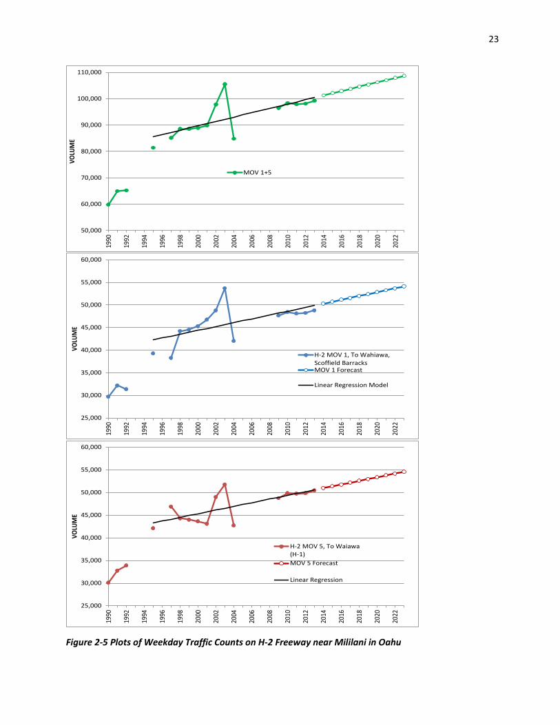
23
Figure 2-5 Plots of Weekday Traffic Counts on H-2 Freeway near Mililani in Oahu
50,000
60,000
70,000
80,000
90,000
100,000
110,000
1990
1992
1994
1996
1998
2000
2002
2004
2006
2008
2010
2012
2014
2016
2018
2020
2022
VOLU
ME
MOV 1+5
25,000
30,000
35,000
40,000
45,000
50,000
55,000
60,000
1990
1992
1994
1996
1998
2000
2002
2004
2006
2008
2010
2012
2014
2016
2018
2020
2022
VOLU
ME
H-2 MOV 1, To Wahiawa,Scoffield BarracksMOV 1 Forecast
Linear Regression Model
25,000
30,000
35,000
40,000
45,000
50,000
55,000
60,000
1990
1992
1994
1996
1998
2000
2002
2004
2006
2008
2010
2012
2014
2016
2018
2020
2022
VOLU
ME
H-2 MOV 5, To Waiawa(H-1)MOV 5 Forecast
Linear Regression

24
Figure 2-6 Output from Excel's Regression Tool for the H-2 Freeway
First the R2 = 36% shows substantial correlation between time and volume. Volumes increase when going forward in time, as would be expected. The F test suggests that one or more of the model’s independent variables are meaningful. (Technically, the F test shows that the “residual sum of squares”, or the amount of noise in the data series after applying the model, is significantly less than the “total sum of squares”, or the amount of noise in the data series originally, given the number of variables used to estimate the model.) The t-statistic for the intercept and slope are also statistically strong, with well over 95% confidence in each of them being different than zero. It should also be noted that the model contains 10 or more years of data, which is desirable. The model is deemed to be statistically reliable for short term forecasts, which are also shown on the graphs. The models suggest that in ten years this section of the H-2 Freeway will be carrying about 55,000 vehicles per day per direction. This level of traffic is sufficiently high to warrant additional analysis of the freeway’s capacity.
2.3.3 Example 3: An Autoregression Model with Box-Cox Transformation The following example was developed from the same original data used in NCHRP Report 765 that was first published by Savage (1997).1 The example in this section goes beyond what is contained in NCHRP Report 765 by using more years of data and including an optional Box-Cox transformation within the autoregression. This example was developed entirely within Excel using its Analysis ToolPak. This section illustrates the most sophisticated analysis that can be accomplished within these guidelines.
Table 2-1 shows monthly ferry ridership counts over a six year period of time.
1 Joseph P. Savage, “Simplified Approaches to Ferry Travel Demand Forecasting”, Transportation Research Record: Journal of the Transportation Research Board, Number 1608, 1997, pp. 17-29.
SUMMARY OUTPUT
Regression StatisticsMultiple R 0.642R Square 0.412Adjusted R Square 0.359Standard Error 5139Observations 13
ANOVAdf SS MS F Significance F
Regression 1 203971301 2.04E+08 7.723 0.018Residual 11 290513997 26410363Total 12 494485298
Coefficients Standard Error t Stat P-value Lower 95%Intercept 83278 4037 20.627 0.000 74391.9047X Variable 1 722.051 259.819 2.779 0.018 150.194

25
Table 2-1 Ferry Traffic Count Data (Savage, 1997)
Month Year 1 Year 2 Year 3 Year 4 Year 5 Year 6 January 2593 2374 2469 2848 2465 3464
February 2345 2474 2513 2502 2555 3095 March 2948 2000 2546 2814 3446 4035
April 4282 4387 4035 4350 4797 5295 May 5744 5668 5612 5656 6059 6790 June 7449 7441 7283 7623 8440 9286 July 8706 8971 8659 9263 10819 11294
August 9966 9588 8200 9949 11904 11672 September 7982 7848 7713 7680 8949 9221
October 5507 5703 6072 6147 6896 7000 November 4744 4428 4095 4737 5322 5605 December 3500 4673 4288 4665 5040 5241
Visual observations of the time series (Figure 2-7) would suggest that there is a yearly cycle to the data and that the variation within a year is growing slowly over time. These observations imply that an autoregressive model would need at least two lag terms and that there might be some advantage to a Box-Cox transformation.
Figure 2-7 Monthly Ferry Counts (Vehicles)
0
2000
4000
6000
8000
10000
12000
14000
Jan-
91
Jan-
92
Jan-
93
Jan-
94
Jan-
95
Jan-
96
Jan-
97

26
The count data series is divided into thirds (two full years in each), transformed, and checked for similarity of standard deviations. Table 2-2 shows the results of five different values of β (1.0, 0.8, 0.5, 0.3, 0.0). For example, the transformation for a value of β = 0.5 for the very first month (January of Year 1) is accomplished by this calculation:
𝑇0.5 =25930.5 − 1
0.5= 99.84
And the transformation for a value of β = 1 for this same month is:
𝑇1.0 =25931.0 − 1
1.0= 2592
Notice that the standard deviations between values of β are quite different from each other, since the data series transformations are quite different from each other.
Table 2-2 Standard Deviations of the Count Data Series Transformations
β 1 0.8 0.5 0.3 0 Early Third 2446 438.5 33.74 6.160 0.4874 Middle Third 2306 413.0 31.66 5.755 0.4514 Late Third 2896 497.5 35.91 6.284 0.4667
The most consistent standard deviations occur with a value of β = 0.3, but none of the inconstancies are obviously bad to the point where they will distort the forecast. The use of a Box-Cox transformation could be bypassed for these data; however, a transformation with a value of β = 0.3 will be continued throughout this example in order to further illustrate the concept.
Table 2-3 lists the autocorrelations for the transformed counts at the first 14 lags. A single lag is a one month offset. The autocorrelations confirm what can be gleaned from graph of counts. The highest autocorrelation is with lag 12 (exactly one full year earlier) with fairly strong autocorrelations also at lags 11 and 13. There is a strong autocorrelation at lag 1, as is typical of count data, and there is another strong, but negative, autocorrelation at lag 6. The reasons for these autocorrelations seem fairly obvious. The graph does not suggest a need to do smoothing, so there are only a few possibilities for sets of independent variables in an AR model, such as:
• AR(1) with a lag at 1; • AR(1) with a lag at 12; • AR(2) with lags at 1 and 12; • AR(3) with lags at 1, 12 and either 11 or 13; • AR(2) with lags at 1 and 6.
Table 2-3 Autocorrelations of the Transformed Counts through the First 14 Lags
Lag Autocorrelation
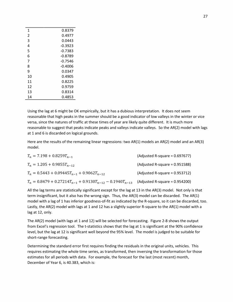
27
1 0.8379 2 0.4977 3 0.0443 4 -0.3923 5 -0.7383 6 -0.8789 7 -0.7546 8 -0.4006 9 0.0347 10 0.4905 11 0.8225 12 0.9759 13 0.8314 14 0.4853
Using the lag at 6 might be OK empirically, but it has a dubious interpretation. It does not seem reasonable that high peaks in the summer should be a good indicator of low valleys in the winter or vice versa, since the natures of traffic at these times of year are likely quite different. It is much more reasonable to suggest that peaks indicate peaks and valleys indicate valleys. So the AR(2) model with lags at 1 and 6 is discarded on logical grounds.
Here are the results of the remaining linear regressions: two AR(1) models an AR(2) model and an AR(3) model.
𝑇𝑛 = 7.198 + 0.8259𝑇𝑛−1 (Adjusted R-square = 0.697677)
𝑇𝑛 = 1.205 + 0.9855𝑇𝑛−12 (Adjusted R-square = 0.951588)
𝑇𝑛 = 0.5443 + 0.09445𝑇𝑛−1 + 0.9062𝑇𝑛−12 (Adjusted R-square = 0.953712)
𝑇𝑛 = 0.8479 + 0.27214𝑇𝑛−1 + 0.9130𝑇𝑛−12 − 0.1940𝑇𝑛−13 (Adjusted R-square = 0.954200)
All the lag terms are statistically significant except for the lag at 13 in the AR(3) model. Not only is that term insignificant, but it also has the wrong sign. Thus, the AR(3) model can be discarded. The AR(1) model with a lag of 1 has inferior goodness-of-fit as indicated by the R-square, so it can be discarded, too. Lastly, the AR(2) model with lags at 1 and 12 has a slightly superior R-square to the AR(1) model with a lag at 12, only.
The AR(2) model (with lags at 1 and 12) will be selected for forecasting. Figure 2-8 shows the output from Excel’s regression tool. The t-statistics shows that the lag at 1 is significant at the 90% confidence level, but the lag at 12 is significant well beyond the 95% level. The model is judged to be suitable for short-range forecasting.
Determining the standard error first requires finding the residuals in the original units, vehicles. This requires estimating the whole time series, as transformed, then inversing the transformation for those estimates for all periods with data. For example, the forecast for the last (most recent) month, December of Year 6, is 40.383, which is:

28
𝑇 = (1 + 0.3𝑇0.3)1 0.3� = (1 + 0.3 ∗ 40.383)1 0.3� =5320 vehicles
The traffic count for that same month was 5241 vehicles, so the residual is (5241-5320) = 79 vehicles. The population standard deviation of all the residuals is 554 vehicles, which is very close to the standard error of the estimate of 569 vehicles. A spot check of the all residuals indicates that the model is doing a good job at matching the cyclic pattern in the data and that the model is not biased with respect to time.
Figure 2-8 Output from Excel’s Regression Tool for an AR(2) Model of Ferry Traffic with Lags at 1 and 12
Just as a validity check, a similar AR(2) model can be easily estimated on the original, untransformed, data. The estimated equation is:
𝑇𝑛 = 67.01 + 0.09360𝑇𝑛−1 + 0.9384𝑇𝑛−12 (Adjusted R-square = 0.954543)
with a standard error of the estimate of 569 vehicles, obtained directly from the output of the regression analysis. The transformed and untransformed AR(2) models are nearly identical, except for the constant term.
In order to forecast with the transformed AR(2) model, it is necessary to forecast all time periods beyond the end of the data until the forecast period is reached. So, for example, if a forecast is desired for December of Year 8, there is also a need for forecasts for November of Year 8 and December of Year 7. Similar logic applies to all earlier time periods. The earliest forecasted time periods can use some real data for independent variables, but eventually all independent variables are forecasts, themselves.
Table 2-4 shows all the transformed data necessary to forecast December of Year 8. The columns for Year 7 and Year 8 are all forecasts. There is no need for any real data prior to Year 6, because the largest lag is 12 months.
Table 2-4 Transformed Data for Year 6 and Transformed Forecasts for Years 7 and 8
Month Year 6 Year 7 Year 8 January 35.1039 36.1525 37.1732
SUMMARY OUTPUT
Regression StatisticsMultiple R 0.977385025R Square 0.955281487Adjusted R Square 0.953712416Standard Error 1.347019871Observations 60
ANOVAdf SS MS F Significance F
Regression 2 2209.361925 1104.681 608.8199 3.45851E-39Residual 57 103.4243644 1.814463Total 59 2312.786289
Coefficients Standard Error t Stat P-value Lower 95% Upper 95% Lower 95.0% Upper 95.0%Intercept 0.544254807 1.201620319 0.452934 0.652316 -1.861948376 2.95045799 -1.86194838 2.95045799X Variable 1 0.094449143 0.049353402 1.913731 0.060681 -0.00437934 0.193277626 -0.00437934 0.193277626X Variable 2 0.906238361 0.050170702 18.0631 2.94E-25 0.805773264 1.006703458 0.80577326 1.006703458

29
February 33.8268 34.6139 35.4237 March 36.9042 37.2576 37.6542
April 40.3221 40.6047 40.8982 May 43.7037 43.9853 44.2682 June 48.3353 48.5020 48.6797 July 51.4607 51.7609 52.0497
August 52.0045 52.5615 53.0936 September 48.2266 49.2134 50.1580
October 44.1355 45.1897 46.2342 November 41.0737 42.0349 43.0047 December 40.1881 40.9344 41.7023
The forecast for December of Year 8 was accomplished by this calculation:
𝑇𝑛 = 0.5443 + 0.09445 ∗ 43.0047 + 0.9062 ∗ 40.9344 = 41.7023
And applying an inverse transformation to this transformed forecast gives a result of 5874 vehicles. The 50% confidence interval for this forecast is:
𝐸50 = ±0.6745 ∗ 569 = ±384
2.4 Special Reporting Requirements Reports of statistical model estimations and forecasts should contain these elements, at a minimum:
• List and description of data sources; • Any data cleaning to remove anomalies; • Any required interpolation because of missing data; • Brief mention of any associated techniques (e.g., smoothing and transformations) that would aid
understanding of how the analysis progressed. • List of variables and coefficients; • Confidence level used to select independent variables into the regression equation or minimum
t-scores; • Adjusted R-square; • Standard error of the estimate; • Forecast(s), baseline and/or with optional scenarios.
There is no need to report individual t-scores for independent variables, so long as each t-score meets minimum requirements.
A graph of the traffic count data series may or may not be helpful in communicating results, depending upon data quality. Anomalies or missing counts may convey a sense of weakness in the database, even when the model is statistically strong.
A graph of the trend line, with additional lines to indicate confidence intervals or scenarios, may be an effective communications tool.

30
Details of the forecast that are of limited value to the public or that are unnecessary for archival purposes may be omitted. Such details include the software used, specifics of how the software was set up, or variables that were tried and rejected.

31
3 Evaluation 3.1 Measures of Effectiveness and Performance Measures Measures of effectives (MOEs) are direct outputs of travel models to gauge the amount of travel for an alternative and to understand the alternative’s impacts. Performance measures relate directly to transportation plan objectives and give an indication about whether the plan’s objectives and goals are being attained, once implemented. Performance measures should preferably be calculated from real-world data. It is possible for a travel forecasting model and its post-processors to compute MOEs that resemble performance measures. This section will deal mainly with MOEs.
Standard MOEs from travel models include vehicle-hours-travel and vehicle-miles-traveled. These two MOEs may be broken out by functional class and/or by location. Other easily computed MOEs are total hours of delay and average speed. Travel models may also be able to roughly estimate air pollution emissions from vehicles, greenhouse gas emissions, and fuel consumption.
Caution needs to be exercised when interpreting MOEs because travel models do not encompass all possible behavioral responses by travelers. For example, a travel model might suggest that fuel consumption would decline with a lowering of delays at signals. However, if the travel model does not include feedback to the distribution step or if the travel model does not include a land-use component, then offsetting increases in trip length owing to reduced delays at signals would not have been accounted for in the total fuel consumptions estimates.
3.2 Refinement for Evaluation 3.2.1 Refining Vehicle Class Forecasts for Evaluation Several of the methods in this chapter depend upon having good vehicle class forecasts. Very often forecasts are done for all vehicles together or for aggregations of vehicle classes. Forecasts may be “refined” as to their vehicle classes by using a technique from NCHRP Report 255 (Chapter 11 of the “Users Guide”) and NCHRP Report 765 (Section 9.3). See Section 5.3.3 for a brief introduction. Essentially, this technique employs data from recent classification counts in order to factor broad truck (or total vehicle) categories into narrower truck categories. Classification data from the exact highway being analyzed are preferred to data from similar locations or data from regional-wide averages. The analyst should follow these steps (as an expansion and application of Step 4 from Section 5.3.3).
• Step 1. Obtain classification counts for the highway(s) being forecast. Counts should be tabulated by FHWA vehicle classes.
• Step 2. Identify the vehicle classes in the original forecast by associating each class with one or more FHWA vehicle classes.
• Step 3. Identify the vehicles classes in the refined forecast by associating each class with one or more FHWA vehicle classes.
• Step 4. Using the classifications counts from Step 1, calculate the proportion of vehicles in each FHWA vehicle class.
• Step 5. Calculate the portion of each original class (Step 2) to be associated with each refined class (Step 3).
• Step 6. Apply the proportions in Step 5 to each original class forecast to obtain FHWA vehicle class forecast(s).
• Step 7. Aggregate FHWA vehicle class forecasts to obtain the refined forecasts, as necessary.

32
Table 3-1 illustrates this concept on a hypothetical Highway AA where the original forecast follows the Quick Response Freight Manual and the refined forecast will be used for the purpose of establishing ESALs for a repaving project. (See Section 3.3.4)
Table 3-1 Example of Converting QRFM Categories to Hawaii Pavement Design Categories
FHWA Vehicle Class Description
FHWA Vehicle Type
QRFM Category (Step 2)
Hawaii Pavement Category (Step 3)
Percent of Truck + Bus (Step 4)
Percent of QRFM Category (Step 5)
Motorcycle 1 * Automobile 2 Automobile Automobile 100.00 Pickup, Panel, Van 3 4-Tire Automobile 100.00 Bus 4 Bus 7.06 * 2 Axle Truck, Single Unit 5 Single Unit 2 Axle 42.04 75.41 3 Axle Truck, Single Unit 6 Single Unit 3 Axle 13.46 24.14 4+ Axle Truck, Single Unit 7 Single Unit 4-Axle 0.25 0.45 3,4 Axle Truck, 1 Trailer 8 Combination 4-Axle 12.22 39.23 5 Axle Truck, 1 Trailer 9 Combination 5 Axle 15.01 48.19 6+ Axle Truck, 1 Trailer 10 Combination 6 Axle 2.31 7.41 5 Axle Truck, 2+ Trailer 11 Combination 5 Axle 0.00 0.00 6 Axle Truck, 2+ Trailer 12 Combination 6 Axle 0.05 0.16 7+ Axle Truck, 2+ Trailer 13 Combination 6 Axle 1.56 5.01 *Not applicable
For the example of Table 3-1, the QRFM forecast is refined by the computations shown in Table 3-2.
Table 3-2 Refining an Example QRFM Forecast to Match Hawaii Pavement Categories
FHWA Vehicle Class Description
Hawaii Pavement Category (Step 3)
Percent of QRFM Category (Step 5)
QRFM Forecast, Highway AA
Forecast for Pavement Category (Step 6)
Aggregated Categories (Step 7)
Motorcycle * * Automobile Automobile 100.00 8257 8257 10807 Pickup, Panel, Van Automobile 100.00 2550 2550 Bus Bus * 2 Axle Truck, Single Unit 2 Axle 75.41 712 712 3 Axle Truck, Single Unit 3 Axle 24.14 944 228 228 4+ Axle Truck, Single Unit 4-Axle 0.45 4 189 3,4 Axle Truck, 1 Trailer 4-Axle 39.23 185 5 Axle Truck, 1 Trailer 5 Axle 48.19 227 227 6+ Axle Truck, 1 Trailer 6 Axle 7.41 472 35 35 5 Axle Truck, 2+ Trailer 5 Axle 0.00 0 0 6 Axle Truck, 2+ Trailer 6 Axle 0.16 1 25 7+ Axle Truck, 2+ Trailer 6 Axle 5.01 24 *Not applicable

33
The QRFM forecast for Highway AA gives traffic volumes for four vehicle classes: automobiles = 8257 vpd; 4-tire trucks = 2550 vpd; single-unit trucks = 944 vpd; and combination trucks = 472 vpd. There is no need to disaggregate 4-tire trucks since all of them will be combined with automobiles in Step 7. Single-unit trucks must be disaggregated into 2-axle, 3-axle, and 4-axle trucks (FHWA classes 5, 6 and7). A similar disaggregation needs to occur for combination trucks (FHWA classes 8, 9, 10, 11, 12 and 13). As the last step, similar FHWA vehicle classes (7+8 and 12+13) are aggregated.
3.2.2 Refining Speeds for Evaluation Some post-processors used for evaluation require speeds at different times of day. Ideally, speeds should be estimated hour-by-hour within a travel model or by further analysis of hourly traffic volumes from another forecasting methodology. It is not possible to obtain hourly speeds directly from multihour (or 24-hour) forecasted volumes. If multihour speeds are needed, they should be calculated as the volume-weighted average of speeds across all hours in the time period.
3.3 Conventional Post-Processing 3.3.1 Highway Noise Analysis Highway traffic noise analysis is usually performed with FHWA’s Traffic Noise Model (TNM). The TNM has five built-in vehicle classes that are roughly compatible with the Quick Response Freight Manual: motorcycles, automobiles + light trucks, medium trucks, heavy trucks, and buses. Traffic inputs consists of hourly volumes and speeds for each class for each road segment. Segments in the TNM are directional, so traffic volumes must also be directional. See Section 5.3.2 for a recommended procedure for creating directional splits by time of day from bidirectional forecasts. There also may be a need for traffic volumes by lane for input to the TNM; however, traffic volumes by lane on multilane facilities are not commonly available as outputs from traffic forecasting methodologies. Other data sources must be used.
TNM also requires estimates of speed. It is recommended that speeds be obtained from post processing, rather than taken directly from travel forecasting software, unless the travel model derives its speeds from operational analysis procedures from the Highway Capacity Manual (or similar quality traffic flow relationships). Vehicle class refinement may be necessary to forecast traffic volumes for each of the five TNM standard classes or for any special classes. See Sections 5.3.3 and 3.2 for details. It is further recommended that classification counts include motorcycles (FHWA vehicle type 1).
Noise standards are in units of LEQ in FHWA’s Noise Abatement Criteria. Certain noise calculations available in the TNM, specifically Ldn, and Lden, may require separate volume forecasts for daytime, evening, and nighttime. The use of these noise measures would be considered unusual in Hawaii. Evening is defined as the hours between 7PM and 10 PM. Nighttime is defined as the hours between 10 PM and 7 AM. Unless the travel forecast is very complete in its treatment of times of day, there will be a need to perform post-assignment time-of-day factoring to convert 24-hour volumes to two or three of these time periods. See Section 5.3.2 for details. Speeds must also be estimated for multihour periods of time. See Section 3.2.2.
3.3.2 Safety Analysis Safety impacts of a highway project are closely associated with the change in VMT and the crash rate per vehicle mile. In addition, the crash rate may differ across facilities within a project, or the crash rate might vary by alternative. (ASK GORO about intersections????)

34
3.3.3 User Benefits Benefit/cost analyses for highway projects, apart from safety considerations, rely most heavily on travel time savings and travel distance savings for user benefits. Travel time savings are converted to dollars by multiplying by a value of time. Values of time vary by vehicle class and user class. Values of time for personal travel and for non-freight commercial vehicles are pegged to the prevailing wage rate. Values of time (as well as values of distance) for freight vehicles are based on the costs of truck operation.
Travel time savings are estimated from the difference between VHT (vehicle-hours-travel) before and after the project. Travel distance savings are estimated from the difference between VMT (vehicle-miles-travel) before and after the project. VHT and VMT are standard outputs of the traffic assignment step in travel model. Ideally, the traffic assignment step is “multiclass”, thereby giving VHT and VMT separately for each vehicle class with unique values of time and values of distance. In the absence of a “multiclass” traffic assignment, it is possible to refine traffic volumes into vehicle classes by using the methods outlined in Sections 5.3.3 and 3.2. Values of time are not considered to be affected by highway functional class.
BCA.Net is a benefit/cost analysis tool for highway projects that is maintained by FHWA. BCA.Net needs peak and off-peak AADT traffic volumes and the proportion of vehicles in each of three vehicle classes: automobiles, truck, and buses. Separate peaking and vehicle mix profiles may be defined for weekdays and weekend days.
Most traffic forecasts do not calculate VHT and VMT by user class (e.g., by income or by travel purpose). If desired, estimates of VHT and VMT by user class would require (given outputs from conventional travel model) a post-processing step. For example, VHTs and VMTs may be refined into purposes with trip production rate percentages from NCHRP #365 (Table 9), pre-assignment time-of-day factors from NCHRP 716 (Table C.11), and known average trip lengths (either from a traffic model or from survey data) appropriate for the community. BCA.Net does not differentiate between user classes.
Using net VHT and net VMT for user benefits assumes that the total number of trips within the system is constant. Another, more robust, measure of user benefits, utilized by BCA.Net, is consumer surplus. Consumer surplus, as implemented in many transportation studies, may be a more appropriate means of estimating user benefits than strict travel time/cost savings when there is an increase (or decrease) in the number of trips within the analysis area.
3.3.4 Pavement Design Hawaii currently uses its own procedure for pavement design, but it resembles the traditional AASHTO procedures as to traffic inputs. The major traffic input to both the traditional AASHTO procedures and Hawaii’s procedures is equivalent single axle loads (ESALs). The Hawaii procedure first converts ESALs per vehicle to ESALs per vehicle per year, called ESALCs. Total ESALs are computed from knowledge of which type of trucks are in the traffic stream, how those trucks are loaded, and how many of those trucks are forecasted to traverse that road segment from the opening year to the design year. A total value for ESALs over all vehicle classes is specific to a single lane in one direction on a specific road segment. Additional data on lane distribution and directional split are required. The analyst may assume that the number of ESALCs for a single truck of a standard type has already been computed.
Forecasts may be for all traffic together or broken out by vehicle class. In either case, there is a need convert forecast data into standard vehicles for computing ESALCs and then total ESALs. Hawaii uses the

35
vehicle classes in Table 3-3 when finding total ESALs. The table also gives example ESALCs, but these values may be subject to change. Light-duty trucks with 4 tires (while not in commercial service) should be categorized with automobiles for pavement design.
Table 3-3 Vehicle Classes for Pavement Design Purposes in Hawaii with Illustrative ESALC values
Vehicle Class Description FHWA Vehicle Type Approximate ESALCs per Truck* Automobile 2 None (ESAL ≈ 0.0004) Bus 4 450 2 Axle Truck 5 30 3 Axle Truck 6 420 4 Axle Truck 7, 8 600 5 Axle Truck 9, 11 850 6 Axle Truck 10, 12, 13 950 Source: Draft Pavement Design Manual, 2007.
Depending upon the traffic forecasting methodology, there may be inconsistencies between the vehicle classes from the traffic forecast and vehicle classes needed for pavement design. For example, traffic forecasts following the Quick Response Freight Manual (either edition), breaks trucks into just three vehicle classes: four-tire trucks, single unit trucks of 6 or more tires, and combination trucks. See Section 3.2 for details on how to resolve such inconsistencies.
The Mechanistic-Empirical Pavement Design Guide (MEPDG), not yet adopted in Hawaii, also requires forecasts of traffic volumes by vehicle classes. However, the MEPDG requires speeds. Speeds from travel models using operational analysis procedures from the Highway Capacity Manual (or similar) are suitable for pavement design purposes. Otherwise, speed forecasts may need to come from post-processing.
3.3.5 Air Quality, GHG Emissions and Energy Consumption All of Hawaii is in attainment of the national ambient air quality standards (NAAQS) from the Clean Air Act, so there is little need for air quality analysis for highway projects.
For guidance on estimating GHG emissions from HPMS data or from travel models, see FHWA’s, “Handbook for Estimating Transportation Greenhouse Gas Emissions for Integration into the Planning Process”. The methods presented in this Handbook are largely based on obtaining good VMT and speed estimates for a whole region. Emission factors may be improved by introducing a customized vehicle mix in MOVES. Although written for GHG gases, the advice in this Handbook applies equally well to the process of estimating energy consumption from highway vehicles.
3.4 Traffic Microsimulation Software implementations of the Highway Capacity Manual are suitable for obtaining post-processed speeds from traffic forecasts. However, traffic microsimulations may be used to provide much more refined outputs of speeds and travel times in and near a highway project with unusual geometry or complicated arrangements of traffic controls. True hybrid models, which involve traffic microsimulations, are discussed in Section 6.2.1. Speed and travel time refinements are described in Section 5.3.6.
Traffic microsimulations are considered superior to travel models in their estimates of delays, but microsimulations may be costly. It is important that any traffic microsimulation be set up such that

36
turning movements are identical to the traffic forecast. Since results from traffic microsimulations vary from run to run, it is important to repeat any given simulation several times with different random seeds.
Traffic microsimulations can provide other indicators of traffic performance, such as queue lengths, and microsimulations can precisely pinpoint the location of potential traffic problems. Traffic microsimulations can also provide a good evaluation of the suitability of specific traffic controls.
3.4.1 List of Acceptable Traffic Analysis/Microsimulation Software The following software packages are acceptable for post-processing results from a traffic forecast:
• Highway Capacity Software • Mainstream microsimulatgions CORSIM, Paramics, Vissim
Software documentation should be consulted for the proper use of each product and the interpretation of the product’s outputs.
3.5 Land Use Models Several major metropolitan areas in the US have integrated land-use models into their travel forecasts. The latest generation of land-use models require extensive and spatially-detailed data on the economy of the region. A well-functioning land-use model will forecast the spatial distribution of population and employment by economic sector. These models are expensive and time-consuming to set up and calibrate. Land-use models are especially important for regions that are rapidly developing and are testing major alternatives to greatly improve highway and transit accessibility to parts of the region that are now less intensively developed. However, land-use models have not undergone the level of validation as have traditional four-step travel forecasting models, so there is still considerable uncertainty in the planning community as to the quality of those forecasts. It is very important that an analyst be advised by outputs of land-use models, where available, but land-use models are of only limited value for project-level travel forecasting.
3.6 Special Reporting Requirements MOEs are often more aggregated than individual traffic volumes, so percent of random error in any MOE may be less than the percent of random error in a single traffic volume forecast. However, the amount of error in any MOE is difficult to estimate, so there is no expectation that error ranges be reported for MOEs.
Reporting requirements differ across MOEs. At a minimum, the analyst should report the name and version of any software product, the nature of any travel forecasting inputs, the source of any parameters, a description of any assumptions, and a succinct statement of the MOEs, preferably in tabular form.

37
4 Case Studies All the examples in this chapter relate to building case study analyses using actual data from HDOT to illustrate various models presented in the chapters above.
4.1 Case Study 1 – Based on the Lahaina Bypass 4.1.1 Introduction The subject forecast is based on various parts of actual studies conducted by HDOT concerning the Lahaina Bypass project, which bypasses the Honoapiilani Highway through Lahaina Town on the island of Maui. The actual project is currently under development with one phase completed and others in progress. A forecast requesting form was developed for the purposes of this case study.

38
STATE OF HAWAII DEPARTMENT OF TRANSPORTATION
HIGHWAYS DIVISION TRAFFIC FORECAST REQUEST FORM
I. PROJECT NH-030_1(44)
II. DATA REQUESTED A. FORECAST YEARS ☐ Current Year: 2012 ☐ Open-to-Traffic Year: Click here to enter text. ☑ Design Year: 2032 ☐ Plan Horizon Year: Click here to enter text. ☐ Other Year: Click here to enter text. B. DETAILS ☑ Volume (hourly or ADT) ☑ Truck Percentage ☐ Vehicle Mix ☑ Directional
☐
☐ Origin-Destination Table
☐ Turning Movements (specify or attach map) Click here to enter text. ☑ Other (specify or attach map) Please include data for pavement design. C. ANALYSIS TIME PERIODS ☑ 24-
☑ Design ☐ AM Peak ☐ PM Peak ☐
Click here to enter text. D
MEASURES OF EFFECTIVENESS ☐ Vehicle miles traveled ☐ Vehicle hours traveled ☐
Click here to enter text.
III. APPLICATION ☑ Intersection Geometric Design Changes ☐ Signalization Changes ☐ Access Management ☐ Lane Widening ☐ Road Diet ☐ Other Cross-Section Modification ☐ New
☐ Detour/Diversion Analysis for Work Zones
☐ Travel Demand Management ☐ Site Impact ☑ New Pavements ☐ Programming
☐ General
☐ Public Information ☑
IV. LOCATION AND SITE DESCRIPTION Route Number (s) and/or Road Names Honoapiilani Highway Realignment, Phase 1C, Kaanapali
C t t K St t E t i Milepost Begin (if
Milepost End (if applicable) Click here to enter text. Geographical Extent of Study Area (if more than one facility) Click here
enter text.
Title

39
☐ See Study Area Map Location Description Click here to enter text.
Land-Use Description and Site Developments Click here to enter text. ☐ See Land Use or Site Map
V. ALTERNATIVES ☐ Do
☐ Build 1 (describe) Click here to enter text. ☐ Build 2 (describe) Click here to enter text. ☐ Build 3 (describe) Click here to enter text. ☐ See Alternatives Map (optional)
VI. SPECIAL REQUIREMENT Click here to enter text.
VII. ADDITIONAL DESCRIPTIONS OF PROJECT, SITE OR ENVIRONMENT (OPTIONAL) Click here to enter text.
VIII. MAPS AND ATTACHMENTS (OPTIONAL) ☑ Location
☐ Site
☐ Alternative
☐ Other Click here to enter text. IX. NEED BY DATE
1/10/13 X. ACCOUNTING
F YR APPR D S/D OBJ FUNC C/C S
XI. REQUESTED BY
Name John T. Requester Telephone 808-8888 E-mail Click here to enter text. Date of Request 10/25/12
XII. ADMINISTRATIVE RECORD (FOR PLANNING BRANCH USE ONLY) Analyst’s Name Click here to enter text. Date
10/30/12
Forecast Reference Number TA 1234
12 401 D 434 1122 1K653

40
4.1.2 Tool Selection The characteristics of available resources and desired data to be forecasted determine what tools need to be employed. Section 1.5 “Tools Selection Matrix for Hawaii” formalizes the logic used to aid in this decision. Here it is used accordingly to identify suitable forecasting tools. The Lahaina Bypass project forecast matches the following characteristics from the matrix:
Planning/Design • New corridors/facilities – both rural and urban • ESALs/load spectra
Operations • Detour/diversion analysis, for lane closures, road closures or work zones
Geography • Small area (includes single intersections)
Forecast Output Requirements • Intersection turning movements • Traffic volumes (ADT, peak hour, peak period, all hours) • Select link O-Ds
Time Horizon • Long range
Technical Resources • Statewide travel model, outputs only • Recent Mainline Traffic Counts (also by vehicle class) • Historical traffic counts • Existing and proposed geometry
The matrix produced the following scores.
DTA guidelines, TOD Post assignment (includes peak spreading), TOD K factors, and Model results factoring (including Turning Movement adjustments) appear to be most suitable for this forecasting request.

41
4.1.3 Tool Application The data available for this location do not include any origin-destination data sets or models; thus. a full model with dynamic traffic assignment (DTA) cannot be built. There is detailed information on ADT of the only existing route at this location (Honoapiilani Hwy.) as well a past study based on a regional demand forecasting model that includes forecasts between the existing route and the proposed Lahaina Bypass. For use in this study it is assumed that the split factors were obtained in the last five (5) years. If the factors (the splits by direction between existing road and proposed bypass) are old or non-existent, then for relatively compact bypasses a traffic study should be executed to determine the splits, as explained in section 6.4.2.
4.1.3.1 ADT Regression Forecasts of Honoapiilani Hwy. There is a large gap in the data between 1994 and 2002. A past attempt at a forecast introduced an interpolation technique and, in fact, introduced data not in evidence and produced the red line forecast. It is preferred to use only the data available to estimate a linear regression model (blue line forecast.) While the actual estimates may be close, the model with the interpolated data usually comes with inflated values of statistical significance.
In this case the model with the interpolated data points has R2=0.82 and a standard error of estimate equal to 1200, whereas the model with the original data has R2=0.45 and SEE equal to 2400. Both models have statistically significant parameters for the constant and the slope, 8.6 and 9 for the interpolated data model, and -2.8 and 2.9 for the original data model.
0
5,000
10,000
15,000
20,000
25,000
30,000
35,000
40,000
45,000
50,000
1990 1995 2000 2005 2010 2015 2020 2025 2030 2035
Volu
me
(veh
/day
)
Year
Regression Forecast, MP 20.93-22.26
Case Study Forecast
Original Data
Old Data
Old Forecast

42
ADT Splits, 2012 to Maalaea to KaanapaliHonoapiilani Hwy. 8,595 11,823Lahaina Bypass 10,938 6,944Sum and share, below 19,533 18,767Honoapiilani Hwy. 44% 63%Lahaina Bypass 56% 37%
ADT Splits, 2032 to Maalaea to KaanapaliHonoapiilani Hwy. 10,123 13,925Lahaina Bypass 12,883 8,178Directional sum 23,006 22,104Total cross section ADT 45,110
The year 2032 forecast ADT is 45,110 for the model with original data and 47,483 for the model with interpolated data, a difference of +5.3%.
4.1.3.2 Old and New Route Splits The next major question requiring an answer through forecasting is the portion of the traffic that will split onto either the existing highway or the new bypass. In this case there are data available from a regional model but they are over five years old. As a result a traffic survey was conducted.
Section 6.4 explains that if an alternate route is proposed around a small section of a busy highway to bypass a village, a major tourist attraction, a shopping center, etc., a special traffic observation study can be setup to observe vehicles at a cross-section location U upstream and D downstream of a busy location L. License plate recognition or Bluetooth ID recognition technology can be used to assess vehicles traveling from U to D and from D to U through L. Vehicles that spent more than twice the average time to traverse the segment had some reason to “visit” L and they would stay on this route if a bypass was built. The ratio of "visit"-to-"bypass" by time of day is a reliable basis for developing the demand profile of the proposed bypass route by time of day and direction based on the ADT profile of the existing route through L.
Bluetooth (BT) sensors were placed at the two extremes of the project as shown in the aerial depiction slide above. The two day 24-hour data indicate that the daily directional split is almost even, with 51% of the BT matches recorded on the direction to Maalaea and 49% on the direction to Kaanapali.
The BT data indicate that 44% of those on the direction to Maalaea will likely continue to use Honoapiilani Hwy. because they were either not-re-identified (i.e., their destination was Lahaina town) at the exit station or they did after the criterial travel time had passed (i.e., they did have some short term business in Lahaina town.) The same statistic for the other direction is much higher at 63% indicating the large number of tourists arriving from Kahului and Kihei to visit Lahaina town. With these two shares on hand the rest of the shares are the balance to 100% and reflect the portion that is expected to use the Lahaina Bypass.
If it were here, the Lahaina Bypass, would have approximately 11,000 ADT on the direction to Maalaea and 7,000 ADT on the direction to Kaanapali. Currently all this traffic is served by Honoapiilani Hwy.
In 2032 the Lahaina Bypass is expected to have 13,000 ADT on the direction to Maalaea and 8,000 ADT on the direction to Kaanapali.
NOTE THAT ALL THESE TABULATED NUMBERS REPRESENT FICTITIOUS BLUETOOTH OR LICENSE PLATE SURVEY DATA FOR DEMONTRATING THE METHOD FOR ESTIMATING ROUTE SPLITS. THE FORECASTS OF THIS CASE STUDY CANNOT BE COMPARED WITH ACTUAL FORECASTS OF THE PROJECT.

43
4.1.4 Case Study Recommendations
• Bypasses are best analyzed with complete forecasting models such as a DTA model combined by split and time of day factoring.2
• Forecasts of main/bypass splits from regional models should be based on data that are at most five (5) years old.
• If splits are too old or unavailable, they should be determined empirically at the field via an observational methodology based on license plate recognition or Bluetooth re-identification technology.
• Original data should be relied upon and interpolations between original data should be kept to a minimum.
• Unless extraordinary conditions are present such as Hurricane Iniki, a multiday strike by a major airline, or a national calamity such as 9-11-2001, years with somewhat large or low data values should not be excluded or modeled with a dummy variable because useful variance is lost from the analysis.
• Experienced statisticians of the HDOT should be consulted before a decision to omit a data value as “junk” is made. A comparison with a similar route on the same island may help detect that a data point is not “junk” if a similarly extreme value is also observed at other traffic station(s).
2 For example, a study in the UK pertaining to a bypass with a projected ADT in the order of 30,000 which is similar to the ADT levels of Honoapiilani Highway included a full forecasting model. A380 South Devon Link Road (Kingskerswell Bypass), June 2009, http://www.devon.gov.uk/kkbp-dccp4.pdf .

44
4.2 Case Study 2 – Based on the Saddle Road - West Side Defense Access Road (Daniel K. Inouye Highway)
The subject forecast is based on actual study conducted in year 2010 by HDOT concerning the Saddle Road - West Side project on the island of Hawaii. The forecast estimated ADTs on the proposed new road and its major intersections in year 2031. The actual project is complete and opened to the public on September 7, 2013 as Daniel K. Inouye Highway.
A description of the original HDOT forecast follows, and then the forecast is compared with new data. Suggestions for improvements are offered.

45
4.2.1 Original HDOT forecast of Saddle Road - West Side, conducted Sept. 2010 We begin with the original forecast request shown on the pictures scan. The following data were requested:
“Current” ADT (year 2011)
Design ADT (year 2031)
DHV (Design Hourly Volume)
T24 (24-hour truck %)
K (peak hour % of 24-hour traffic) - Design only
D (Directional distribution) - Design only
T (Design hour truck %) - Design only
The intended use of the forecast data was for Design geometrics. The project location and alignment were indicated using the maps on the title sheet from the Preliminary 70% drawings. The forecast request was made on Tue. 9/21/10 with the desired due date of Fri. 10/1/10 indicated (10 calendar days, or 8 working days for a Mon-Fri work-week). The work was assigned to a single analyst on Thurs. 9/23/10. The forecast was reviewed/approved by two others, with final completion on Tue. 9/28/10. Assuming a Mon-Fri work week, the work required about 3-4 person-days.
The forecast was done for the build and no-build case. In addition, a short segment of Mamalahoa Highway (Route 190) was considered due to localized improvements. As a result, the forecast has three parts, Part 1, Part 2a, and Part 2b: Part 1 was the improved segment of Saddle Road; Part 2a includes a short segment of Mamalahoa Highway (Route 190) surrounding the intersection with the improved Saddle Road (Route 200); and Part 2b was the same segment of Mamalahoa Highway in the no-build condition.

46

47
The title sheet from project plans, containing maps and parts of the forecast are shown above. Part 1 is a completely new facility, so no historical data are available for it. A regional model including the proposed new road was available from a study conducted in 2002 by Julian Ng, Inc., with forecasts for years 2005 and 2025 shown below.
In year 2008, the forecast appears to have been updated, based on this 2002 study and related correspondence of 2003 (not shown here). An agreement was reached with CFLHD3 using the updated values shown below. The revised values started at 3,500 veh/day in year 2008, and used the following annual growth rates: 2.89% in years 2009-2012, 3.5% in years 2013-2016, and 4% in 2017 onwards.
The values in the figure on the right were the best estimates available and thus accepted without any adjustment (besides the normal rounding to the nearest 100 vehicles). These are the same values reported on the title sheet of the Preliminary 70% drawings.
3 Central Federal Lands Highway Division.

48
Then, in the Preliminary 70% plans (see figure below) the forecast for Part 2a (Mamalahoa Highway) was taken at the intersection with the old leg of Saddle Road; but it should have been taken at the intersection with the improved leg. So a new forecast for Mamalahoa Highway was developed, using historical data (creating Part 2b of the forecast), then adjusted for the additional traffic due to the new road (Part 2a).
In Part 2b, a linear regression of historical data was used to project the ADT up to year 2031, as shown above. The regression was adjusted for “low” years (1998 and 1999).
Then, for Part 2a, based on the study by Julian Ng (2002), 63% of traffic on Saddle Road would take the new branch, so it would flow on Mamalahoa Highway at the location of interest. The difference in 5-year growth rate was used to find the proportion of said 63% that would be added. That is:
(added traffic on Mamalahoa) = [(Saddle Rd. growth rate)-(Mamalahoa growth rate)] x (Saddle Road traffic) x 0.63
Then,
(Part 2a traffic) = (Part 2b traffic) + (added traffic on Mamalahoa)
4.2.2 2015 Comparison with New Data The HDOT forecast from year 2010 is compared with actual volume data now available.
Part 1 contains a short segment of Saddle Road up to the fork, and then the rest of it is the new leg of Saddle road. It should be noted that the forecast assumed the traffic on Saddle would be split into 63% on the new leg and 37% on the old leg, however the way the Part 1 was reported, the entire 100% of

49
traffic on Saddle Road was assigned to it (perhaps due to a practice of choosing the highest traffic segment when it varies along a road). In this case the practice paid off, as it was observed that approximately all the traffic on Saddle Road is taking the new leg in year 2014. In fact, 24-hour traffic counts on it slightly exceed those taken on the same day (April 1 and 2, 2014) near the Pohakuloa Training Area, before Saddle Road splits into the old and new segments. Possible sources of the additional traffic may include traffic coming from the old Saddle Road to avoid using the lower-speed older segment, and entrances to the Pohakuloa Training Area past the counting station.
Given new actual counts, the forecast of about 4,200 vehicles per day is roughly 20% higher than the 2014 observed level of about 3,500.

50
The bar graphs above compare forecast traffic on new and existing segments compared with counts taken on April 1-2, 2014. It appears that the absolute volume of traffic was overestimated by roughly 1,000 vehicles/day. There is not enough data yet to determine the accuracy of the rates of growth.
Growth in traffic on Mamalahoa Highway was overestimated, as shown in the graphs above and below. Actual traffic in this segment had fallen as of year 2013. Data is not yet available for evaluation of Part 2a.
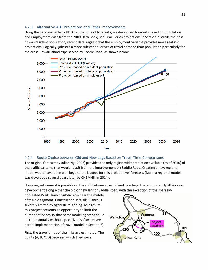
51
4.2.3 Alternative ADT Projections and Other Improvements Using the data available to HDOT at the time of forecasts, we developed forecasts based on population and employment data from the 2009 Data Book; see Time Series projections in Section 2. While the best fit was resident population, recent data suggest that the employment variable provides more realistic projections. Logically, jobs are a more substantial driver of travel demand than population particularly for the cross-Hawaii-island trips served by Saddle Road, as shown below.
4.2.4 Route Choice between Old and New Legs Based on Travel Time Comparisons The original forecast by Julian Ng (2002) provides the only region-wide prediction available (as of 2010) of the traffic patterns that would result from the improvement on Saddle Road. Creating a new regional model would have been well beyond the budget for this project-level forecast. (Note, a regional model was developed several years later by CH2MHill in 2014).
However, refinement is possible on the split between the old and new legs. There is currently little or no development along either the old or new legs of Saddle Road, with the exception of the sparsely-populated Waikii Ranch Subdivision near the middle of the old segment. Construction in Waikii Ranch is severely limited by agricultural zoning. As a result, this project presents an opportunity to limit the number of nodes so that some modeling steps could be run manually without specialized software; see partial implementation of travel model in Section 6).
First, the travel times of the links are estimated. The points (A, B, C, D) between which they were

52
estimated are shown on the map.
To obtain data for developing travel times, it is recommended that the analyst review any capital improvement plans and virtually drive through the segment using the latest available HDOT photolog imagery, or Google Street View if imagery in unavailable. It can be seen that the old Saddle Road has received new pavement but still contains numerous low-speed areas along the series of one-lane bridges with a 20-mph zone, such as the one shown below. The image below depicts virtually driving Saddle Road in the year 2010 condition; note one-lane bridges and limited sight distance due to undulating terrain.
Speed limits of Saddle Road in year 2010 were obtained by virtually driving it in the photolog. The speed limit and mileage were noted whenever the photolog vehicle passed a speed sign. The speed limit was assumed apply immediately from the instant the vehicle passes a sign until it passes the next speed limit sign. The travel time from the fork in Saddle Road to its intersection with Mamalahoa Highway by taking the old Saddle Road versus by taking Daniel K. Inouye Highway and Mamalahoa Highway were then estimated. The speed limit of Mamalahoa Highway was 50 mph in this area. The speed on the Daniel K. Inouye Highway was assumed to be 55 mph. Using speed limits only, the following travel times were estimated as follows.

53
From these estimates, it is apparent that taking the route of Daniel K. Inouye Highway and Mamalahoa Highway is faster in all cases. Based on Wardrop’s equilibrium theory, drivers use the route resulting in the lowest cost to themselves (in this case measured by travel time). These travel times suggest that for all practical purposes, 100% of the traffic at the split at point A will use the Daniel K. Inouye Highway. In contrast the Ng study suggests that 63% will do so.
It should be noted that intersection delays and congestion delays were not accounted for. The effect of delays at intersections, such as yielding/stopping for oncoming traffic at several one-lane bridges, would be expected to increase the travel time of the old Saddle Road more than on the Daniel K. Inouye Highway, which for the most part benefits from uninterrupted flow. Volume/travel time curves were not developed for each link. This project represents a special case where one route clearly dominates; considering the results already obtained and lack of required data, developing volume-delay functions for each link would have been both expensive and unnecessary. Development of volume-delay would be required if a highway improvement were not so drastic or if an area was affected by significant congestion.
Once traffic reaches the intersection at Mamalahoa Highway it needs to be split north-south or into right and left turns.
Given the absence of OxD data in this case (and in many cases for rural projects throughout Hawaii), alternative data may be used as substitutes. In this case population, employment or the hospitality inventory given that a very large part of the ADT at this location on Saddle Road are hotel workers residing in Hilo and working on the west side of the Big Island.
(a) Hawaii Tourism Authority, 2010 hospitality unit inventory Kohala/Waimea/Kawaihae = 4665 units N and S Kona =5182 units These data suggest an almost even split of 53% left turn (south) and 47% right turn (north).
(b) 2010 Census population from CH2MHill study N. Kohala = 1980 S. Kohala = 5940 N. Kona =13050 S. Kona = 3410 These data suggest a split of 67% left turn (south) and 33% right turn (north). However, the
population on north and south Kona does not likely drive the ADT on Saddle Road.
(c) 2007 Census employment from CH2MHill study N. Kohala = 780 S. Kohala = 10600 N. Kona =21340 S. Kona = 2140 These data too suggest a split of 67% left turn (south) and 33% right turn (north) because they
reflect the workers in north and south Kona (thus, not surprisingly, they yield a number similar to that for population) but not many of these workers are likely to use Saddle Road.
In this case capacity and left turn bay analysis should be done assuming that the left lane of the Daniel K. Inouye Highway at Mamalahoa caries 50% to 60% of the westbound ADT.

54
4.3 Case Study – Trend Analysis on Major Highways The objective of this case study is to conduct ADT trend analysis with data from ten highway data stations on Oahu. For each data location, we suggest short term (5 years) growth rates, by direction of travel. The examples below demonstrate the use of methodologies described in this report and they are not necessarily usable recommendations for forecasting, unless the data station ADT volumes used are deemed to be both reliable and representative for this purpose. This study did not filter HDOT data from the sample stations below to ensure that they are representative and reliable for actual forecasts.
4.3.1 Station 724A H-1 Fwy. at McCully St. Overpass
Forecast recommendation: The range of values shows some unusual spikes in late 2008 and early 2009 possibly related to the recession occurring at the same time frame. If regression models are run starting in mid-2009, after the noted anomaly, then the EB model has a slope of practically zero (and the slope coefficient not statistically significant.) Thus for EB traffic the recommendation is for no growth.
The WB direction exhibits growth for both the 2007 to 2010 and the 2009 to 2015 data series, and the coefficient of the slope is statistically significant (t-stat =4.03, a=1%, N=68) based on analysis of data from mod-2009 to mid-2015. An annual growth factor of 0.5% is recommended.

55
4.3.2 Station SL-58. H-1 Fwy. at Kapiolani Interchange
Forecast recommendation: This location exhibits substantial post 2009 recession growth on the WB direction. A large portion of the WB volume at this location exits at the Kapiolani, University and Wilder ramps. The coefficient of the slope is statistically significant (t-stat =4.92, a=1%, N=60) and suggests an annual growth of 1.8%; however a reduced value of 1% annual growth is recommended because part of the growth is likely due to the recovery from the 2009 recession.
The coefficient of the slope is also statistically significant (t-stat =2.4, a=2%, N=60) for the EB direction. This suggests an annual growth of 0.8%, however a reduced value of 0.5% annual growth is recommended.
This site was also used to run periodic ARIMA models for the 60 month period from January 2010 to December 2014. ARIMA (1,0,0)(0,1,1) 12 was specified in SPSS and error analysis indicated a very good fit. ARIMA models were run separately for EB and WB directions. They are plotted on the next page along with their 95% upper and lower confidence intervals. Although ARIMA takes longer to run than a regression, the model fit is clearly superior and it accounts for the periodicity of monthly ADT.
The ARIMA model predicts a 0.46% annual growth on the EB direction between 2011 and 2019, and a 0.93% annual growth on the WB direction between 2011 and 2019. These are more reliable estimates than the 0.8% and 1.8% predicted by the regression growth extrapolation model. When reliable monthly ADT data are available, the periodic ARIMA model is a superior tool for short term forecasts.
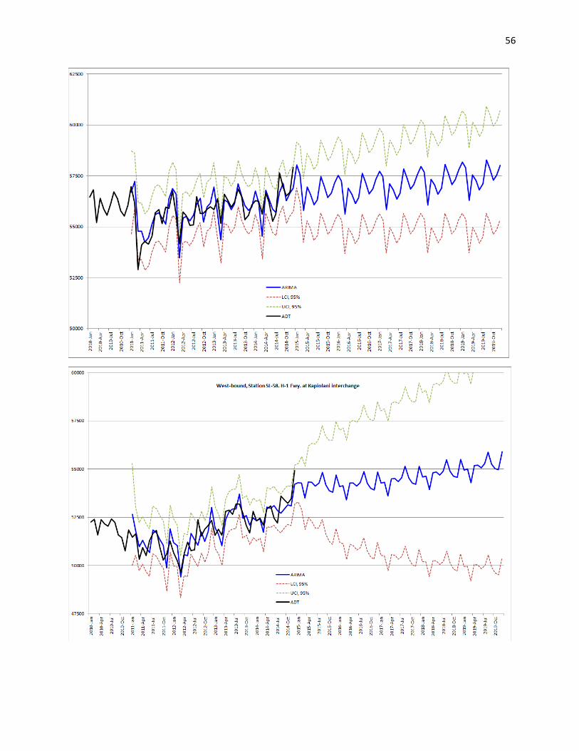
56
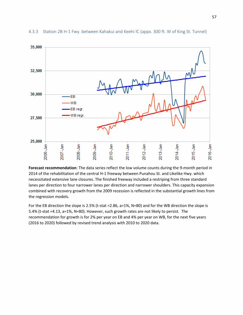
57
4.3.3 Station 2B H-1 Fwy. between Kahakui and Keehi IC (appx. 300 ft. W of King St. Tunnel)
Forecast recommendation: The data series reflect the low volume counts during the 9-month period in 2014 of the rehabilitation of the central H-1 freeway between Punahou St. and Likelike Hwy. which necessitated extensive lane closures. The finished freeway included a restriping from three standard lanes per direction to four narrower lanes per direction and narrower shoulders. This capacity expansion combined with recovery growth from the 2009 recession is reflected in the substantial growth lines from the regression models.
For the EB direction the slope is 2.5% (t-stat =2.86, a=1%, N=80) and for the WB direction the slope is 5.4% (t-stat =4.13, a=1%, N=80). However, such growth rates are not likely to persist. The recommendation for growth is for 2% per year on EB and 4% per year on WB, for the next five years (2016 to 2020) followed by revised trend analysis with 2010 to 2020 data.

58
4.3.4 Station C6-U Moanalua Fwy 0.2 mi W of Kahupaani St. Overpass
Forecast recommendation: EB traffic on Moanalua Fwy. exhibits a statistically significant growth in ADT with a slope of 2.7% (t-stat=3.87, a=1%, N=80). WB traffic on Moanalua Fwy. exhibits a statistically significant declining volume trend with a slope of -2.5% (t-stat=4.36, a=1%, N=80). A +2% annual growth rate for EB and a -2% annual growth rate for WB are recommended for the next five years (2016 to 2020) followed by revised trend analysis with 2010 to 2020 data.

59
4.3.5 Station C7L - H-1 Fwy 200 ft. West of Kaonohi St.
Forecast recommendation: Due to both freeway and rail construction, this section is experiencing wide fluctuations. As Kamehameha Hwy. is increasingly being restricted by rail construction, this section of the freeway will experience variable growth. Although a volume decrease is shown between mid-2010 and mid-2015, the volume trend is flat is 2007 and 2014 are compared. An annual growth rate of 1% per year is recommended for the next decade along with re-assessment once rail construction along Kamehameha Hwy. is completed. (Also see next two pages.)

60
4.3.6 Station 006 Kamehameha Hwy at Kalauao Bridge
Forecast recommendation: This section of Kamehameha Hwy. will experience dramatic fluctuations in volume generated by multiple lane closures of rail guideway and overhead station construction. Forecast estimates are not possible until all rail construction is complete in this section and the final revised lane channelization is delivered for use. Due to the permanent rail infrastructure, some loss of left lanes is expected and narrower through lanes may be designed. Overall this arterial will likely lose 10% or more of its capacity, so a reduction of its ADT may occur post rail completion. However, a reduction in long trips along this section of Kam. Hwy. may be offset by an increase by short trips to serve the two rail stations.

61
4.3.7 Station H-1 Fwy. and Kam. Hwy. Combined at Kaonohi St.
Forecast recommendation: The post-2009 data regression suggests a statistically significant rate of annual reduction of 1%. Both directions have nearly identical combined-volume trend lines with slope statistics as follows: t-stat=2.8, a=1%, N=53. A no growth forecast is recommended for the next five years followed by a revision after the completion of rail construction in this area. EB traffic should be taken at 146,500 ADT and EB traffic should be taken at 142,500 ADT.

62
4.3.8 Station H-3 Fwy. at Halawa
Forecast recommendation: The post 2008-2009 recession volumes on H-3 freeway reveal a no growth pattern on the EB direction (to Kaneohe); the coefficient of the slope is not statistically significant (t-stat=0.29, a=23%, N=68). Given the minimal potential for growth and expansion on Ohau’s windward side, a 1% growth for the next ten years is recommended.
Regression analysis indicates a statistically significant slope of growth in the order of 2.3% for the WB direction. The coefficient of the slope is statistically significant (t-stat=7.3, a=1%, N=68). A 1% annual growth rate is recommended for the next five years (2016 to 2020) followed by revised trend analysis with 2010 to 2020 data.

63
4.3.9 Station 023 - Likelike Highway 400' North of Valley View Drive
Forecast recommendation: Post 2008-2009 data suggest a statistically significant growth pattern on both directions of the Likelike Hwy. with EB growing at 2.2% (t-stat=8.8, a=1%, N=66) and WB growing at 1.5% (t-stat=7.9, a=1%, N=66) per year. For forecasting purposes a 1.5% annual growth rate for each direction is recommended for the next five years (2016 to 2020) followed by revised trend analysis with 2010 to 2020 data.

64
4.3.10 Station 323 Pali Hwy. at Tunnel No.1 (Honolulu Side)
Forecast recommendation: Traffic volume on the Pali Hwy. is steady on the EB direction with a non-significant slope coefficient. For the next decade a constant ADT value of 21,000 is recommended.
Traffic volume on the Pali Hwy. on the WB direction has a statistically significant (t-stat=4.8, a=1%, N=69) negative slope coefficient suggesting an annual 0.5% rate of decline. However, for the next decade a constant ADT value of 21,500 is recommended.

65
4.4 Case Study – Models Correlating ADT with Other Trends The objective of this case study is to explore and develop statistical correlations between ADT and potential explanatory factors such as gross state product, employment rates, gasoline price, and vehicle registrations for forecasting applications. The examples below demonstrate the use of methodologies described in the report and they are not necessarily usable recommendations for forecasting, unless the data station ADT volumes used are deemed to be both representative and reliable for this purpose. This study did not filter HDOT ADT data from the sample stations below to ensure that they are reliable and representative for actual forecasts.
4.4.1 Three Screen Lines Oahu Freeways
Annual data at three freeway screen lines basically show no growth between 2008 and 2015 (Oct. to Dec. 2015 data were extrapolated.) H-1 at Kaonohi did not show any reduction during the 2009 recession. A correlation with gross state product is possible, but none should be expected with vehicle registrations.
500,000
600,000
700,000
800,000
900,000
1,000,000
1,100,000
1,200,000
1,300,000
1,400,000
1,500,000
0
50,000
100,000
150,000
200,000
250,000
2008 2009 2010 2011 2012 2013 2014 2015
Oah
u Ve
hicl
e Re
gist
ratio
ns
ADT
and
GSP
in M
illio
ns
H-3 at Halawa
H-1 at McCully St. OP
H-1 at Kaonohi Ave.
Gross State Product, Million 2009$
Oahu vehicle registrations

66
Regression StatisticsMultiple R 0.970336R Square 0.941551Adjusted R 0.934245Standard E 289.098Observatio 10
ANOVAdf SS MS F ignificance
Regression 1 10770825 10770825 128.8721 3.27E-06Residual 8 668621.2 83577.66Total 9 11439447
Coefficientstandard Erro t Stat P-value Lower 95%Intercept 18269.95 406.2054 44.97714 6.59E-11 17333.24X Variable 3.118448 0.2747 11.35218 3.27E-06 2.484988
4.4.2 Three Non-freeway Screen Lines
The annual profiles of three non-freeway sites show several patterns. The data from Sand Island Access Road cover only five years and show a strong annual growth. The data from Queen Kaahumanu Highway near the Kona International Airport and the data from Saddle Road on the Big Island of Hawaii show volume reductions in the recession years after 2008 and followed by volume increases. Other trends plotted include Hawaii’s gross state product in constant dollars, Oahu vehicle registrations, gasoline price, unemployment rate and the Standard & Poor’s stock market index.
Regression of annual ADT at the Queen Kaahumanu Highway station shows an excellent correlation with the S&P index. This correlation explains past trends, but reliable forecast values of the S&P index are not available, thus the usefulness of the S&P index as a forecasting variable for ADT is limited.
0.00
1.00
2.00
3.00
4.00
5.00
6.00
7.00
8.00
-
5,000
10,000
15,000
20,000
25,000
30,000
35,000
40,000
45,000
50,000
55,000
60,000
65,000
70,000
75,000
2006 2007 2008 2009 2010 2011 2012 2013 2014 2015
Veh.
Reg
in m
illio
ns, G
as $
/gal
, % U
nem
pl.,
S&P
in th
ousa
nds
ADT
and
GSP
(mill
ion
2009
$)
Queen K @ Kona AirportSaddle RoadSand Island Access RoadGross State Product, Million 2009$Oahu vehicle registrations in millionsGasoline priceUnemployment rateS&P 500 in thousands
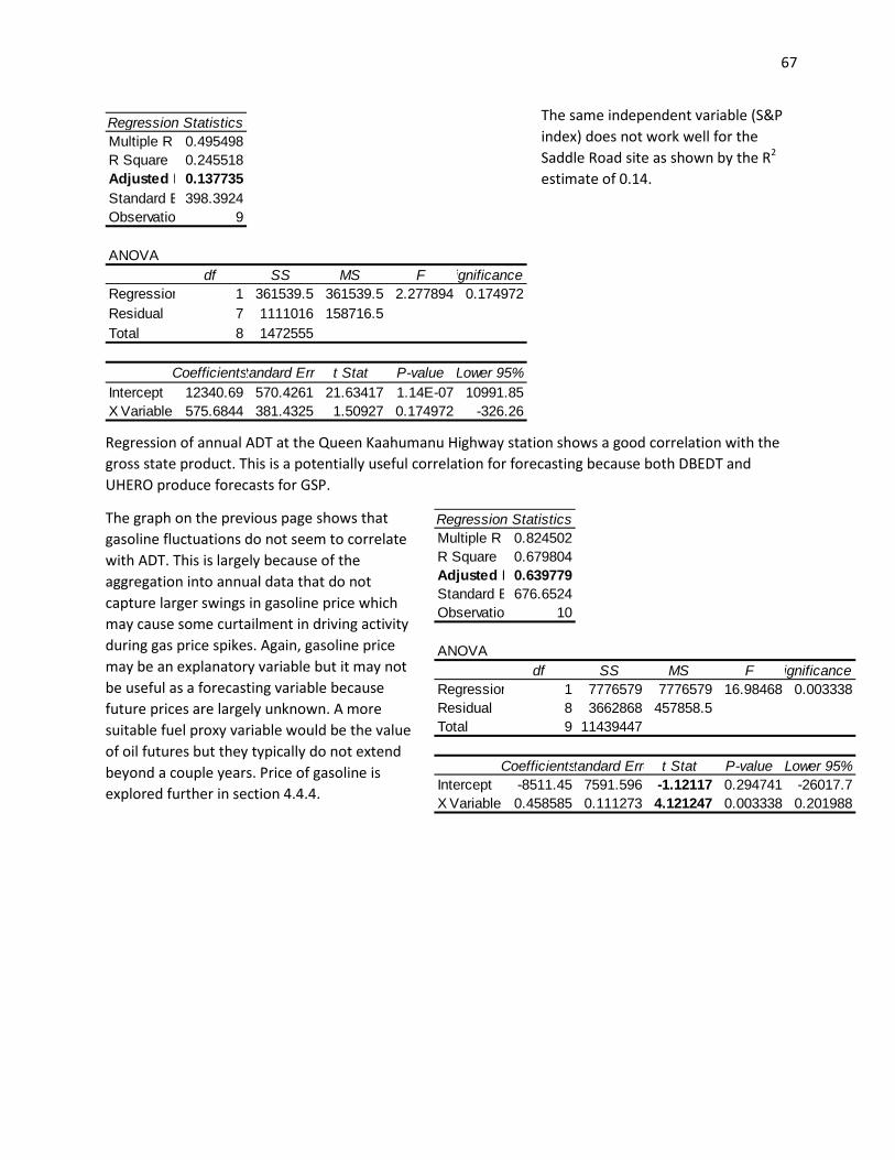
67
The same independent variable (S&P index) does not work well for the Saddle Road site as shown by the R2 estimate of 0.14.
Regression of annual ADT at the Queen Kaahumanu Highway station shows a good correlation with the gross state product. This is a potentially useful correlation for forecasting because both DBEDT and UHERO produce forecasts for GSP.
The graph on the previous page shows that gasoline fluctuations do not seem to correlate with ADT. This is largely because of the aggregation into annual data that do not capture larger swings in gasoline price which may cause some curtailment in driving activity during gas price spikes. Again, gasoline price may be an explanatory variable but it may not be useful as a forecasting variable because future prices are largely unknown. A more suitable fuel proxy variable would be the value of oil futures but they typically do not extend beyond a couple years. Price of gasoline is explored further in section 4.4.4.
Regression StatisticsMultiple R 0.495498R Square 0.245518Adjusted R 0.137735Standard E 398.3924Observatio 9
ANOVAdf SS MS F ignificance
Regression 1 361539.5 361539.5 2.277894 0.174972Residual 7 1111016 158716.5Total 8 1472555
Coefficientstandard Erro t Stat P-value Lower 95%Intercept 12340.69 570.4261 21.63417 1.14E-07 10991.85X Variable 575.6844 381.4325 1.50927 0.174972 -326.26
Regression StatisticsMultiple R 0.824502R Square 0.679804Adjusted R 0.639779Standard E 676.6524Observatio 10
ANOVAdf SS MS F ignificance
Regression 1 7776579 7776579 16.98468 0.003338Residual 8 3662868 457858.5Total 9 11439447
Coefficientstandard Erro t Stat P-value Lower 95%Intercept -8511.45 7591.596 -1.12117 0.294741 -26017.7X Variable 0.458585 0.111273 4.121247 0.003338 0.201988

68
Regression StatisticsMultiple R 0.84267186R Square 0.71009586Adjusted R Sq 0.69456528Standard Erro 619.299438Observations 60
ANOVAdf SS MS F Significance F
Regression 3 52608019.9 17536006.6 45.7224327 4.5039E-15Residual 56 21477780.5 383531.794Total 59 74085800.4
Coefficients Standard Error t Stat P-value Lower 95%Intercept -14300.2105 3656.2889 -3.91112707 0.00025078 -21624.6373GSP 6.45128102 0.63590617 10.1450204 2.7065E-14 5.17740789FEB,MAR 1320.07402 220.069088 5.99845273 1.529E-07 879.222664SEP -1112.80424 292.165603 -3.80881331 0.00034889 -1698.08227
4.4.3 Queen Kaahumanu Highway Station, Monthly ADT Analysis
The stable, post 2009 monthly ADT data from this site are used to demonstrate two models, Model 1 is simply a constant growth model derived by regression and is shown on the left. Its X values are simply 1 for the first month of the data, 2 for the second month of the data, etc. There are data from 60 months in this data set. The model and its parameters are statistically significant.
Model 2 is a multivariate regression model that uses the same volumes as Model 1 for
ADT and three explanatory variables: (1) gross state product, (2) a dummy [0,1] variable representing the months of February and March which are high-ADT months and, (3) a dummy [0,1] variable representing the month of September which is a low-ADT month. These simple and predictable variables yield a very good statistical fit which should be reliable for forecasts. There are data from 60 months in this data set. The model and its parameters are
16,000
18,000
20,000
22,000
24,000
26,000
2006
-Jan
2006
-Jun
2006
-Oct
2007
-Mar
2007
-Aug
2008
-Jan
2008
-Jun
2008
-Nov
2009
-Apr
2009
-Sep
2010
-Feb
2010
-Jul
2010
-Dec
2011
-May
2011
-Oct
2012
-Mar
2012
-Jul
2012
-Dec
2013
-May
2013
-Oct
2014
-Mar
2014
-Aug
2015
-Jan
2015
-Jun
2015
-Nov
Mon
thly
ADT
T8M Queen Kahuumanu Hwy 0.25mi N of OTEC Access Rd. at 9MP Sign (Kona Airport area)
Monthly ADT
MODEL 2
MODEL 1
Regression StatisticsMultiple R 0.72648025R Square 0.52777355Adjusted R Sq 0.51963171Standard Erro 776.655903Observations 60
ANOVAdf SS MS F Significance F
Regression 1 39100525.7 39100525.7 64.8224291 5.0261E-11Residual 58 34985274.7 603194.392Total 59 74085800.4
Coefficients Standard Error t Stat P-value Lower 95%Intercept 21429.6763 203.064824 105.531208 5.4619E-68 21023.1979X Variable 1 46.6138927 5.78965549 8.05123773 5.0261E-11 35.0246381

69
statistically significant. Based on R2, Model 2 improves explanatory power from 52% of Model 1 to 69%.
4.4.4 Koolau Screen Line, Monthly ADT Analysis
Routine monthly data such as gasoline price and unemployment rate are compared with the monthly ADT data at the trans-Koolau screen line that includes both directions of H-3 Freeway, Likelike Highway and Pali Highway combined. The graph above shows four month moving averages, which are easier for
the viewer to follow, but the analysis was done using monthly data.
Unemployment had a small and intuitive correlation producing the result shown on the left. The coefficient for the independent variable has the correct sign, meaning that a high unemployment lowers the ADT. The same analysis for gas price returned a model with R2 = 2% and a positive sign, meaning that high gas prices cause the ADT to increase, which is counter-intuitive.
2.00
2.50
3.00
3.50
4.00
4.50
5.00
5.50
6.00
6.50
7.00
114000
116000
118000
120000
122000
124000
2006
-Jan
2006
-Jun
2006
-Oct
2007
-Mar
2007
-Aug
2008
-Jan
2008
-Jun
2008
-Nov
2009
-Apr
2009
-Sep
2010
-Feb
2010
-Jul
2010
-Dec
2011
-May
2011
-Oct
2012
-Mar
2012
-Jul
2012
-Dec
2013
-May
2013
-Oct
2014
-Mar
2014
-Aug
2015
-Jan
2015
-Jun
2015
-Nov
$/ga
l pric
e of
gas
olin
e on
Oah
u, U
nem
ploy
men
t rat
e
Mon
thly
ADT
Trans-Koolau Screenline (4 month MA)H-3 Fwy, Likelike Hwy, and Pali Hwy
Regression StatisticsMultiple R 0.44599356R Square 0.19891026Adjusted R S 0.19038802Standard Erro 1847.02516Observations 96
ANOVAdf SS MS
Regression 1 79625006.1 79625006.1Residual 94 320681182 3411501.94Total 95 400306188
Coefficients Standard Error t StatIntercept 123098.868 771.212005 159.617417X Variable 1 -656.008785 135.786854 -4.83116564

70
4.4.5 H-1 at Kapiolani Blvd., Monthly ADT Analysis
A number of detailed analyses and two forecasts were conducted with the data from station SL-58. The data in the analysis are shown in the table to the left. Annual data such as GSP and vehicle registrations were transformed in a monthly value based on the % of the annual ADT per month. Their monthly fluctuation was made to follow the monthly fluctuation of volumes. The overall annual growth or decline trend remained the same as in the annual data. This makes the data fit a little better than using the same monthly value for GSP for every month (i.e., [annual GSP]/12).
The regression results on the next page show that a number of correlations were explored. The monthly ADT at this location has
• A weak (R2 = 0.14) but correct (positive) correlation with vehicle registrations.
• A strong (R2 = 0.51) and correct (positive) correlation with gross state product.
• A modest (R2 = 0.35) and correct (negative) correlation with unemployment rate.
• A minimal (R2 = 0.01) but correct (negative) correlation with gasoline price.
When GSP and Unemployment Rate were used in the same model, the coefficient for Unemployment Rate became positive which is counter-intuitive, and thus the model is unacceptable.
When GSP and Gasoline Price were used in the same model, overall model fit became very high at R2 = 0.85 and all parameters have correct signs and are strongly statistically significant based on their t-test values.
Yr-Month ADT Veh.Registr. GSP S&P Unempl Gas Price2010-Jan 108711 91116 5613 1073.87 7.2 3.2812010-Feb 109210 91534 5639 1104.49 6.9 3.3262010-Mar 106782 89499 5513 1169.43 6.9 3.3612010-Apr 108774 91169 5616 1186.69 6.7 3.4382010-May 108019 90536 5577 1089.41 6.7 3.4552010-Jun 107613 90196 5556 1030.71 7.5 3.3642010-Jul 108518 90954 5603 1101.6 7.1 3.3612010-Aug 108936 91305 5625 1049.33 7.0 3.3712010-Sep 107954 90481 5574 1141.2 7.1 3.3142010-Oct 107228 89873 5536 1183.26 6.9 3.3522010-Nov 106280 89078 5487 1180.55 6.9 3.3832010-Dec 107909 90444 5572 1257.64 6.4 3.4652011-Jan 108433 97260 5782 1286.12 6.9 3.5762011-Feb 107786 96680 5748 1327.22 6.7 3.6372011-Mar 103205 92571 5504 1325.83 6.6 3.9592011-Apr 105036 94214 5601 1363.61 6.4 4.3592011-May 104800 94002 5589 1345.2 6.7 4.2582011-Jun 105427 94564 5622 1320.64 7.4 3.9352011-Jul 106212 95268 5664 1292.28 7.0 3.9612011-Aug 107494 96418 5732 1218.89 6.9 4.0112011-Sep 106792 95789 5695 1131.42 7.1 4.0792011-Oct 105426 94563 5622 1253.3 6.9 4.0902011-Nov 106561 95581 5683 1246.96 6.9 4.0062011-Dec 107149 96109 5714 1257.6 6.4 3.9062012-Jan 107427 103440 5782 1312.41 6.8 3.9172012-Feb 105798 101871 5694 1365.68 6.5 4.1012012-Mar 103795 99943 5586 1408.47 6.5 4.3552012-Apr 106348 102401 5723 1397.91 6.2 4.4732012-May 106740 102778 5745 1310.33 6.1 4.4002012-Jun 105834 101906 5696 1362.16 6.8 4.2672012-Jul 105898 101968 5699 1379.32 6.1 4.1282012-Aug 108854 104814 5858 1406.58 5.7 4.1632012-Sep 107164 103187 5767 1440.67 5.8 4.3452012-Oct 107548 103556 5788 1412.16 5.5 4.3342012-Nov 107952 103945 5810 1416.18 5.3 4.0722012-Dec 108309 104289 5829 1426.19 4.8 3.9212013-Jan 107400 106722 5773 1498.11 5.1 4.0052013-Feb 108269 107585 5820 1514.68 4.9 4.2062013-Mar 106731 106057 5737 1569.19 4.8 4.3172013-Apr 109403 108712 5880 1597.57 4.7 4.2992013-May 109167 108478 5868 1630.74 4.6 4.2542013-Jun 108617 107931 5838 1606.28 5.3 4.2322013-Jul 109369 108678 5879 1685.73 4.8 4.2242013-Aug 110031 109336 5914 1632.97 4.7 4.2422013-Sep 109184 108494 5869 1681.55 5.0 4.2052013-Oct 107429 106751 5774 1756.54 5.0 4.0612013-Nov 107247 106570 5765 1805.81 4.9 3.9142013-Dec 108873 108185 5852 1848.36 4.4 3.8192014-Jan 108588 102464 5830 1782.59 4.7 3.8972014-Feb 108705 102575 5836 1859.45 4.6 3.9502014-Mar 107726 101651 5783 1872.34 4.5 4.0952014-Apr 109600 103419 5884 1883.95 4.4 4.2752014-May 109283 103120 5867 1923.57 4.3 4.3442014-Jun 107730 101655 5784 1960.23 5.0 4.3332014-Jul 107833 101752 5789 1930.67 4.5 4.3152014-Aug 111253 104979 5973 2003.37 4.2 4.2772014-Sep 110362 104138 5925 1972.29 4.3 4.1902014-Oct 109726 103538 5891 2018.05 4.1 4.0052014-Nov 110141 103930 5913 2067.56 4.2 3.8502014-Dec 112855 106491 6059 2058.9 3.7 3.557
Station SL-58 (H-1 Fwy at Kapiolani IC)

71
The last model shown was used to produce some short term forecasts based on GSP and gas price values that were available from reliable sources as follows: Annual GSP growth rates were taken from UHERO. Future oil price per barrel was averaged from published reports by the World Bank and the International Monetary Fund. (Forecast oil prices by The Economist Intelligent not were ignored.) The specific values and source links are shown below.
Regression Statistics Regression Statistics Regression StatisticsMultiple R 0.389146 Multiple R 0.719759 Multiple R 0.502863R Square 0.151434 R Square 0.518054 R Square 0.252871Adjusted R 0.136804 Adjusted R 0.509744 Adjusted R 0.239989Standard Er 1599.34 Standard Err 1205.306 Standard Er 1500.707Observations 60 Observations 60 Observation 60
ANOVA ANOVA ANOVAdf SS MS F df SS MS F df SS MS F
Regression 1 26475779 26475779 10.35064 Regression 1 90573032 90573032 62.34533 Regression 1 44210271 44210271 19.6305Residual 58 1.48E+08 2557889 Residual 58 84260292 1452764 Residual 58 1.31E+08 2252122Total 59 1.75E+08 Total 59 1.75E+08 Total 59 1.75E+08
Coefficientstandard Erro t Stat P-value Coefficientstandard Erro t Stat P-value Coefficientstandard Erro t Stat P-valueIntercept 97264.74 3278.256 29.66966 9.41E-37 Intercept 52725.25 6975.665 7.558455 3.38E-10 Intercept 103525.6 981.9575 105.4277 5.78E-68X Variable 1 0.105321 0.032736 3.217241 0.002119 X Variable 1 9.59485 1.215168 7.895906 9.15E-11 X Variable 1 2.883957 0.650913 4.430632 4.23E-05
correct sign correct sign correct sign
Regression Statistics Regression StatisticsMultiple R 0.601037 Multiple R 0.154727R Square 0.361246 R Square 0.023941Adjusted R 0.350233 Adjusted R 0.007112Standard Er 1387.602 Standard Err 1715.285Observations 60 Observations 60
ANOVA ANOVAdf SS MS F df SS MS F
Regression 1 63157786 63157786 32.80174 Regression 1 4185614 4185614 1.422613Residual 58 1.12E+08 1925440 Residual 58 1.71E+08 2942202Total 59 1.75E+08 Total 59 1.75E+08
Coefficientstandard Erro t Stat P-value Coefficientstandard Erro t Stat P-valueIntercept 113235 967.3238 117.0601 1.37E-70 Intercept 110771.8 2509.12 44.14766 2.45E-46X Variable 1 -938.673 163.8951 -5.72728 3.82E-07 X Variable 1 -752.814 631.1669 -1.19273 0.237831
correct sign correct sign
Regression Statistics Regression StatisticsMultiple R 0.720196 Multiple R 0.923582R Square 0.518682 R Square 0.853005Adjusted R S0.501794 Adjusted R 0.847847Standard Er 1215.041 Standard Err 671.47Observations 60 Observations 60
ANOVA ANOVAdf SS MS F df SS MS F
Regression 2 90682882 45341441 30.7124 Regression 2 1.49E+08 74566810 165.3835Residual 57 84150442 1476324 Residual 57 25699704 450872Total 59 1.75E+08 Total 59 1.75E+08
Coefficientstandard Erro t Stat P-value Coefficientstandard Erro t Stat P-valueIntercept 49152.73 14865.2 3.306565 0.001638 Intercept 40790.3 4024.74 10.13489 2.3E-14X Variable 1 10.14149 2.348702 4.317911 6.36E-05 X Variable 1 13.89927 0.775198 17.92997 4.21E-25X Variable 2 75.05855 275.1631 0.272778 0.786009 X Variable 2 -3224.47 282.9318 -11.3966 2.52E-16
GSP and Unemployment rate GSP and Gasoline price
Gas PriceUnemployment rate
Oahu Vehicle Registrations GSP, Million 2009$ S&P Monthly Closing

72
The forecasts shown (red dashed line) below is likely correct if four more years of state growth and diminishing gas prices are realized. However the depicted forecast is likely an overestimate because it is not capacity restrained and congestion effects on both sides of the H-1 freeway may temper some of the predicted growth in ADT. A more reliable model of this form should be based on 140 or more sequential observations (12 years of data.)
UHERO Real GSP http://www.uhero.hawaii.edu/assets/15Q3_State_Update_Public.pdf2015 2.82016 2.22017 1.92018 2.0
Crude oil price trend "US EIA expects 10 cents drop in 2016"WB IMF EIU WB+IMF
2014 96.2 96.2 98.9 96.22015 52.5 51.6 50.2 52.12016 51.4 50.4 69.3 50.92017 54.6 55.4 79.9 55.02018 57.9 59.8 86.4 58.9
knoema.com/yxptpab/crude-oil-price-forecast-long-term-2015-to-2025-data-and-charts

73
5 Interfacing with Models Developed by Partner Agencies 5.1 Standard Models 5.1.1 Ideal Travel Model Standard The “travel model ideal” was defined in NCHRP Report 765. The purpose of the “travel model ideal” was to provide a goal for model developers and to alert practitioners that travel models can satisfy the needs of project-level forecasts, under many circumstances. The “best practical experience model” (see Section 5.1.2) is a more realistic design for travel models in Hawaii that may be used for project-level travel forecasting.
5.1.2 Best Practical Experience Model Standard The “best practical experience model” is a specification of a travel model that can be used for project-level forecasts, with or without the need for a refinement step. The “best practical experience model” uses off-the-shelf technology, but adheres fairly closely to the travel model ideal. The specifications listed below cover highway forecasts, exclusively:
• The ability to estimate demands between all origins and all destinations through behavioral principles, through an O-D table estimated with traffic counts, or both;
• The ability to make adjustments to the O-D table to reflect differences between base-year traffic counts and base-year forecasted volumes;
• The ability to perform dynamic equilibrium traffic assignments, with appropriate feedback to earlier steps, if necessary; and
• The ability to calculate delays for through and turning movements (separately) at traffic controlled intersections according to accepted traffic engineering principles, such as operational analysis procedures from the “2010 Highway Capacity Manual”.
• The ability to incorporate delays from turning movements into traffic assignments. • The ability to apply time-of-day (TOD) factors prior to traffic assignment for peak-hour
assignments. • The ability to handle a fine-grained zone system. • The ability to handle a high level of network detail, including streets of functional classes lower
than minor arterial. • The ability to have multiple vehicle classes to correctly track trucks. • The ability to have multiple driver classes to correctly represent the effects road pricing has on
path choice. (Adapted from the Travel Model Ideal, NCHRP Report 765).
The “best practical experience model” should be capable of obtaining validation statistics close to those in the second column of Table 1-2, which come from a region in the US that is using a similarly constructed model.
5.1.3 Acceptable Practical Experience Model Standard An acceptable practical experience model is typical of the better models used for travel forecasting in the United States. Those models are four-step or activity-based, but only three steps are absolutely required for project-level traffic forecasting. The specification of an acceptable model constitutes minimum expectations as follows:

74
• Ability to perform trip generation with procedures from NCHRP Report 365, NCHRP Report 716 or similar;
• Ability to perform trip distribution with a gravity model or a destination choice model or similar; • Ability to perform equilibrium traffic assignments with feedback to trip distribution; • Ability to assign traffic for a single peak hour using pre-assignment time-of-day factors; and • Meets standards of the “Travel Model Validation and Reasonableness Checking Manual II” and
validates to within the standard of Table 1-2 for traffic volumes in the base case.
5.1.4 Discussion of Travel Delay in Acceptable Models Many travel models in the US calculate delays with a “volume-delay function” (VDF) where travel time on a link is a function of the volume on that same link. An example of a VDF is the well-known “BPR curve”. A much preferred method of calculating delays is to use operational analysis procedures from the “2010 US Highway Capacity Manual” or traffic network microsimulation models. Operational analysis procedures incorporate intersection geometry, signal timing and the effects of opposing and conflicting traffic. If a travel model calculates delays with a VDF, exclusively, then the estimated travel times (or speeds) must be viewed with suspicion, even when the model has been intensively calibrated and can show strong validation statistics. In addition, estimated turning movements will tend to have larger errors when delays are calculated with a VDF. Refinement steps are required when using speed and turning movement results for a project-level forecast from a travel model that depends upon VDFs for travel time estimation.
5.2 Direct Use of Travel Model Outputs 5.2.1 Interpolation between Forecast Years 5.2.1.1 Objective The objective of this technique is to deal with inconsistencies that can arise when outputs of a travel model are for a forecast year that is different from the design year of the project.
This technique applies to forecasts that are interim and long-range. This technique applies to all geographic scopes.
5.2.1.2 Background Many regional travel forecasts are done in 5- or 10-year increments. The design year (or open for traffic year) for a project will not necessarily fall exactly on one of the forecast years for a regional model. Ideally, the regional model should be run for the forecast year of the project, but lead times and budgets do not always allow such custom runs that vary the forecast year. Interpolation may be used to resolve inconsistencies in forecast years.
5.2.1.3 Guidelines These guidelines apply to interpolating regional model volume forecasts.
• A project alternative must be part of the forecast for each of the two years used in the interpolation.
• Unless there is convincing evidence to do otherwise, interpolation should be linear (or straight-line).
• There must not be any other (modeled) projects or actions that occur between the two forecast years that have a significant influence on traffic at or near the project.

75
5.2.1.4 Advice Interpolated volumes should be refined, depending upon the needs of the forecast. Speeds and delays cannot be interpolated. Post-processing is required to obtain speeds and delays for interpolated volumes.
5.2.1.5 Example Figure 5-1 illustrates linear interpolation for a hypothetical repaving project on Highway AA. This segment of Highway AA is four-lane and it runs north and south, but only the traffic forecasts for the northbound lanes are shown. Of particular interest is the open-to-traffic year (2016) and the design-year (2031).
Figure 5-1 Interpolation Example, Highway AA
Neither the open-to-traffic year nor the design year fall exactly on the forecast years for the regional travel model. Linear interpolation requires summing the earlier-year forecast and a fraction of the difference between the later-year forecast and the earlier-year forecast. So for 2016 (open-to-traffic year), the earlier year forecast is 12223, the later year forecast is 12589, and the year 2016 is one-fifth of the time from 2015 to 2020. Therefore, the 2016 interpolated forecast is 12223 + (1/5)*(12589 – 12223) = 12296 vpd. By similar logic, the 2031 design year forecast is 13563 vpd.
5.2.1.6 Items to Report • Interpolated volumes (refined or otherwise) • Interpolated turning movements (refined or otherwise) • Post-processed speeds from interpolated volumes • Interpolated VMT or other MOEs
5.2.1.7 References and Sources NCHRP Report 765.
11000
11500
12000
12500
13000
13500
14000
2015 2020 2025 2030 2035
Traffic Forecast, Highway AA, Northbound
Open-to-Traffic Year
Design Year
12223
12589
13534
13680

76
5.2.2 Pivoting with Select Link Analysis for Small Developments 5.2.2.1 Objective Changes in land development can lead to changes in traffic on road segments within or near a highway project. A regional travel forecasting model may be used to estimate those traffic changes, but such a model may not be sensitive enough to small changes in development. In addition, a regional travel forecasting model may be in substantial error on one or more pertinent road segments. However, if a “select link analysis” is available (or can be made available) for road segments, then it may be possible to find the incremental traffic increases (or decreases) in volumes on those road segments.
This technique applies to forecasts that are short-term. This technique applies to corridors.
5.2.2.2 Background A select link analysis gives the origin-destination flows through a single link; and it can be performed with a regional travel forecasting model. A select link analysis may be repeated for any number of road segments (links). In mathematical notation, a select link analysis reports the number for trips, 𝑇𝑖𝑖𝑎, between zone i and zone j that pass through link a. The forecasted volume 𝐶𝑎on link a is the sum of the whole select-link O-D table.
Often, the focus is upon a single zone’s (z) development. Therefore, the analysis needs to consider only those trips with either an origin or a destination in zone z, 𝑇𝑧𝑖𝑎 or 𝑇𝑖𝑧𝑎 , respectively. Any O-D pairs with a trivial amount of traffic can be ignored.
Furthermore, it is useful to define the fractional increase in trip origins from zone z, 𝑓𝑜 , and the fractional increase in trip destinations from zone z, 𝑓𝑑 . Once these fractional increases have been computed, the incremental increase in a link volume can be found by applying these fractions to the O-D matrix. That is,
Incremental Volume = 𝑓𝑜 �𝑇𝑧𝑖𝑎𝑁
𝑖=1
+ 𝑓𝑑 �𝑇𝑖𝑧𝑎𝑁
𝑖=1
Select link analyses can also serve as a check on volumes estimates by other techniques and provide a better understanding for the reasons traffic might increase within a project.
Determination of fractional increases depends upon the type of development. A zone’s current trip generation may be obtained from a trip generation step within the regional model (best) or from the applications of trip generation rates from national sources such as NCHRP Report 716 or NCHRP Report 365 (second best). Pre-assignment time-of-day factors should be applied to production and attraction estimates to obtain origin and destination estimates. A default set of pre-assignment time-of-day factors may be found in NCHRP Report 716. Increases in trip generation may be found in the same way, or they can be determined by applying rates from ITE’s “Trip Generation.”
5.2.2.3 Guidelines If the regional travel forecasting model is in substantial error in the base year for the selected link’s volume, then, at the analyst’s judgment, the base-case O-D matrix may be scaled to match an existing ground count, 𝐶𝑎. In which case, the scale factor, s, is carried through to the forecast.

77
Scaled Incremental Volume = 𝑓𝑜 𝑠�𝑇𝑧𝑖𝑎𝑁
𝑖=1
+ 𝑓𝑑 𝑠�𝑇𝑖𝑧𝑎𝑁
𝑖=1
The scale factor may be obtained by taking the ratio of the count to the base case forecasted volume, that is:
𝑠 = 𝐶𝑎𝐶𝑎� .
5.2.2.4 Advice This technique assumes that new traffic from a zone is distributed spatially the same way as existing traffic in the zone. If there is reason to believe that new and existing traffic will be considerably different in its origin-destination pattern, then this technique cannot be used.
This technique assumes that traffic re-routing will not occur due to the incremental change in land use. If substantial traffic re-routing could occur, then this technique cannot be used. Total volume forecasts from this technique should be compared with the capacity of road segment(s) to assure that the amount of traffic can be handled without the need for significant rerouting.
It is possible to extend the analysis to development in multiple zones by adding additional zones, z, within the same select link analysis. However, the technique can become unwieldy with too many zones.
The impact of decreases in development may be found by the same technique by using negative values for the “fractional increase”.
If the regional planning model has the capability, select zone analysis may accomplish the same thing. Select zone analysis gives the number of trips on each link that has an origin or destination at a given zone. However, select zone analysis can often be ambiguous as to directionality for links that are tangential to a zone.
If a scale factor is used to adjust the select link analysis to count value, it is best to use statistical techniques (averaging or time series analysis) to establish that count value rather than use a single piece of count data.
5.2.2.5 Items to Report • Geography: selected link(s) and zones with assumed increases in development. • Fractional increases in origins and destinations. • Volume increases on a road segments(s)
5.2.2.6 References and Sources NCHRP Report 765 and NCHRP Report 255.
5.3 Refinement Methods 5.3.1 OD Table Refinements 5.3.1.1 Objective An O-D table refinement improves the fit of a traffic model to ground counts in the base year by making systematic empirical adjustments to an O-D table that had been previously computed from behavioral principles or obtained through a survey. An O-D table refinement has the potential to smooth-out irregularities in traffic counts while achieving a perfectly balanced set of forecasted volumes. There are a

78
large number of methods for refining an O-D table. Refinements can be in the form of additive adjustments or multiplicative adjustments. When creating refinements it is important to preserve as much of the underlying structure of the original O-D table as possible.
This technique applies to short-term and interim forecasts. The technique applies to corridor, small-area and wide area geographical scopes.
5.3.1.2 Background O-D table refinement uses the concept of O-D table estimation with traffic counts. Refinements may be static or dynamic; this section emphasizes static refinements. There are many different methods in the published literature, but they all share certain common elements. An O-D table estimation from traffic counts requires three important data items.
• Seed O-D Table. A seed O-D table is an approximation of the final O-D table. The seed O-D table can be derived from behavioral principles, such as those embedded in a 4-step model, or it can be obtained from surveys, such as home-interviews or vehicle re-identification studies or both. The seed O-D table gives a rough shape to the final O-D matrix. It is desirable that certain properties of the seed O-D table, such as average trip length, should be retained throughout the estimation process.
• Directional Traffic Counts. Traffic counts are needed by direction and for the time period of the forecast. There should be a sufficient number of counts to at least establish row and column factors for the O-D table. That is, the number of counts should be greater than twice the number of zones and external stations. Traffic counts should be provided for all roads leading in or out of the study area.
• Select Link Analyses on All Link Directions with Counts. A set of select link analyses is a required input for the estimation. Except for very small networks with all-or-nothing traffic assignments, the select link analyses must be performed within travel forecasting software. As mentioned in Section 5.2.2 a select link analysis finds the number of trips between zones i and j that pass through link direction a, 𝑇𝑖𝑖𝑎. Knowing the total number of trips between zones i and j, it is possible to compute the proportion of trips between zones i and j that use link direction a, 𝑝𝑖𝑖𝑎 . These proportions are 0 or 1 for an all-or-nothing traffic assignment, but can be any number between 0 and 1 for a multipath traffic assignment, including an equilibrium traffic assignment.
The estimation process attempts to find a balance between distortions to the seed O-D table and mismatches to the traffic counts. One way of achieving this balance is through a minimization process, such as illustrated in this equation:
min𝑃 = �𝑤𝑎 �𝐶𝑎 − 𝑠��𝑝𝑖𝑖𝑎𝑁
𝑖=1
𝑇𝑖𝑖
𝑁
𝑖=1
�
2𝐴
𝑎=1
+ 𝑧���𝑇𝑖𝑖∗ − 𝑠𝑇𝑖𝑖�2
𝑁
𝑖=1
𝑁
𝑖=1
where 𝑤𝑎 are link weights, z is a O-D table weight, s is a scale factor, 𝑇𝑖𝑖∗ is the seed O-D table, 𝑇𝑖𝑖 is the estimated O-D table, and everything else has been defined previously. Estimated O-D flows are constrained to be non-negative. Link weights allow the analyst to emphasize or deemphasize certain counts, perhaps because counts can be uneven in terms of quality. The OD table weight is used to

79
control the amount of distortion in the O-D table, which influences the closeness of fit to the ground counts.
Once the estimated O-D table has been found, corrections can be expressed additively,
𝑅𝑖𝑖 = 𝑇𝑖𝑖 − 𝑇𝑖𝑖∗
or multiplicatively,
𝐾𝑖𝑖 = 𝑇𝑖𝑖𝑇𝑖𝑖∗� .
After performing a forecast with a travel forecasting model, refinements can be reintroduced into the forecast by modifying the forecasted O-D additively or multiplicatively.
Dynamic refinements are similar, but add the time dimension to a static table. Dynamic refinements require traffic counts for each of numerous time periods that are used within a dynamic traffic assignment (DTA), as well as a dynamic seed O-D table.
An important detail with O-D table refinements is the need for feedback between equilibrium traffic assignment and the estimation process. This is often referred to in the literature as a “bilevel optimization”, since some equilibrium traffic assignment methods also use optimization theory. Practically speaking, “bilevel optimization” increases the computational burden of the estimation process, but does not place any significant additional requirement on the analyst.
5.3.1.3 Guidelines Since O-D table refinements, for the most part, require specialized software, the software documentation should be consulted to determine input requirements and interpretations of outputs. However, there are several guidelines for O-D table estimation that generally apply.
• All counts must be directional. Bidirectional counts need to be split by direction using local knowledge.
• All counts must be for the time period of the forecast. If necessary, daily counts can be factored into hourly estimated counts by applying post-assignment time-of-day factors, such as those found in NCHRP Report 765. However, actual counts for the time period of the forecast are preferred to factored counts.
• Traffic counts should be provided at all external stations. If actual counts are not available, then it may be necessary to approximate those counts by (a) adapting counts from a nearby count station on the same road or (b) assuming a count value based on typical values for roads of the same functional class and capacity. Counts that are approximate should be assigned a lower weight in the estimation.
• There must be a sufficient number of counts. The exact number of counts depends on where they are located, but a minimum for good results is twice the number of zones plus external stations.
• Traffic counts should be spread throughout the network. • Counts should be reasonably balanced (that is, conservation of flow should be approximately
correct at all junctions.) In addition, counts which are inconsistent with surrounding counts should be removed.

80
• A target should be established for the desired deviation between counts and estimated volumes. This target should be no smaller than the error in a traffic count (see Section 1.7). Weighting should be adjusted (such as the trip table weight, z) to attain this target. Trial estimations will likely be necessary, because the relationship between weights and deviations cannot be known in advance.
• A decision must be made as to whether the refinement will be additive or multiplicative, if the software allows a choice.
• The resulting O-D table needs to be inspected for reasonableness. Volumes on links without counts, in particular, need to be inspected for reasonableness. Average trip length should be inspected for reasonableness. If available, delays and queue lengths could be inspected for reasonableness.
5.3.1.4 Advice O-D table refinements are preferred over screenline refinements, because they can involve many more traffic counts, and thus, the adjusted screenline volumes are based on a more comprehensive set of information.
Large O-D table refinements can be very computational. It may take hours or days to find a solution on a fast desktop computer for large O-D tables and large networks.
It is recommended that old refinements be updated at intervals of no more than five years.
5.3.1.5 Items to Report • Refinement adjustments (computer file) • Refinement table (computer file) • Report on the stability of O-D table and assignment properties • Goodness of fit to ground counts
5.3.1.6 References and Sources NCHRP Report 765.
5.3.2 Temporal Refinements and Directional Split Refinements 5.3.2.1 Objective The objective of temporal refinement is to reduce the length of the forecast period, often from a 24-hour forecast to an hourly forecast, down to an interval that is more suitable for project-level evaluation. There are two ways of accomplishing this refinement: pre-assignment and post-assignment. Pre-assignment time-of-day factors must be applied within travel forecasting software, but post-assignment time-of-day factors may be applied after a travel model run has been completed. Time-of-day factors may also be used in adjusting traffic counts to a specific time period for an OD table estimation. Dynamic traffic assignments (DTAs) and traffic microsimulations may require O-D tables that are factored into time periods of less than one hour.
Directional split refinements are intended to improve upon directional splits from a regional travel forecasting model or to convert bidirectional volumes to directional volumes.

81
5.3.2.2 Background Many travel forecasting models are set up to provide forecasts for a full 24 hours or for multihour peak periods. However, projects are often evaluated by how well they perform over a single hour, either a design hour or a weekday peak hour. More than thirty years ago, time of day factors were published in NCHRP Report 255 (post-assignment) and NCHRP Report 187 (pre-assignment). The factors have been recently updated in NCHRP Report 765 (post-assignment) and NCHRP Report 716 (pre-assignment). Local factors are preferred to national defaults. Time-of-day factors can also be obtained from ITE’s “Trip Generation”; these factors should be considered to apply post-assignment for site-specific traffic.
Default directional split factors are available from NCHRP 255, but these factors are not recommended for projects in Hawaii.
5.3.2.3 Guidelines The following guidelines relate to time-of-day factoring.
• Locally derived factors are preferred over national defaults. • Factors derived from data for the specific highway being forecasted are preferred over data from
nearby highways or from groups of highways having similar characteristics. • ADT forecasts may be converted to design hour forecasts using standard K factors for the Xth
highest hour. As of this time, Hawaii does not use the Xth highest hour as a design hour for most highways.
• Refer to software documentation for instructions on how to apply pre-assignment time-of-day factors.
• Given the choice of both methods, pre-assignment time-of-day factoring is preferred over post-assignment time-of-day factoring.
• Post-assignment time-of-day factors can be for any hour within a single day or for a design hour. These factors apply to vehicle trips at the time that they pass an individual street segment.
• Post-assignment time-of-day factors are location specific and can vary by functional class, by location type (urban or rural), by urban area size, by day of week and by surrounding land use.
• Pre-assignment time-of-day factors are broken-out by purpose and by direction of travel (to or from the trip production end). Totals of factors for a specific direction should be close to 0.5 or 50%, but they do not need to be exactly 50%. These factors apply to person trips but can vary by the type of vehicle; separate tables in NCHRP Report 716 give factors for “all modes”, “auto modes”, “transit modes”, and “nonmotorized modes”. These factors apply to trips at the time of departure at the origin end (either production end or attraction end, depending upon the direction of travel). Non-home-based factors can be assumed to be the same for both directions of travel.
• Time-of-day tables should be inspected to assure that all the factors add to 1.0 or 100%, within a trip purpose.
• When preparing O-D tables for short time periods or for a DTA application, 24-hour counts may be converted using post-assignment factors. However, counts that are adjusted in this manner should be given a smaller than usual weight in the O-D table estimation process.
• NCHRP Report 765 describes a method whereby hourly time-of-day factors may be interpolated to periods of less than one hour, if necessary for DTAs. The method is given for pre-assignment factors, but the general idea will work for post-assignment factors, as well.

82
• Time-of-day factors for trucks are different from time of day factors for automobiles. Example truck time-of-day factors can be found in NCHRP Report 765 and in FHWA’s original Quick Response Freight Manual from 1996. These factors should be considered to be post-assignment in their application.
Hawaii does not maintain default K and D tables, preferring instead to develop those factors using historical data specific to a highway segment. The following steps should be used for development of post assignment time-of-day factors for individual highway segments having historical traffic count data, but are not continuous counting locations.
1. Obtain weekday traffic counts by 15 minute intervals for the highway segment, in accordance with FHWA’s “Traffic Monitoring Guide”. 15-minute counts from each day of a 48-hour coverage count should be averaged together. It is recommended that counts be obtained for at least 5 separate prior years (but extending no more than 10 years in the past), if possible.
2. Calculate the percent of daily traffic for each possible hour in the day, starting on a whole 15-minute interval for 15-minute counts. This should be done for each direction of a two-way highway. This will result in 96 hourly percentages for each day for a one-way highway and 192 hourly percentages for each day for a two-way highway. These percentages should be calculated to 3 digits past the decimal point, e.g., 8.325).
3. Average these hourly percentages together across years, directionally (i.e., each direction separately) and bidirectionally (i.e., both directions together).
4. The hour starting between 6:00 AM and 11:30 AM with the highest bidirectional average percentage shall be chosen to be the “AM peak hour”. The hour starting between 11:45 AM and 5:30 PM with the highest bidirectional average percentage shall be chosen to be the “PM peak hour”.
5. The AM K factor is the average bidirectional percentage in the AM peak hour. Similarly, the PM K factor is the average bidirectional percentage in the PM peak hour. These factors shall be reported to the nearest tenth of one percent.
6. The ratio of the directional factors or a single hour is the directional split for that hour. The directional split shall be reported to the nearest whole percentage for each direction of travel. The directional split is relative to a specific direction and should not be considered to be valid for both directions of travel.
7. Compare the K factor values (time-of-day) to those from NCHRP Report 765 as a check for reasonableness.
8. Compare the D factor values (directional split) to similar sites as a check for reasonableness.
5.3.2.4 Advice Day-of-week factors may be useful in translating a forecast from a typical weekday to a specific weekday. However, day-of-week factors cannot be established with data from coverage counts. NCHRP Report 765 contains national default day-of-week factors. Day-of-week factors may also be used to convert weekday counts to a specific weekday, with caution.
Day-of-week factors (which are available in NCHRP Report 765) should not be used to convert weekday counts to a specific weekend day, unless there are no other options for obtaining weekend counts.

83
The growing interest in DTA suggests that in the future time-of-day factors should be computed in time increments of less than one hour, such as 15 minutes, from count data.
5.3.2.5 Items to Report • Hourly factors • Hourly directional splits • Factored counts or factored volumes
5.3.2.6 References and Sources NCHRP Report 716 and NCHRP Report 765.
5.3.3 Vehicle Mix Refinements 5.3.3.1 Objective Vehicle mix is defined as the percentage of vehicles within each of many vehicle classes within a traffic stream. Project level decisions often require good knowledge of the number of trucks and the size of trucks, particularly for delay calculations, pavement designs and environmental assessments. Regional travel forecasting models tend to have only a few vehicle types, at best, within a multiclass traffic assignment. Coverage traffic counts, for the most part, do not count trucks separately from passenger cars. Thus, there is a need for factoring traffic forecasts, based directly on counts or otherwise, into many vehicle classes.
5.3.3.2 Background The concept of vehicle mix refinement was first introduced in NCHRP Report 255 and then updated for NCHRP Report 765. It is well known that the percentage of trucks varies considerably with the location (urban/rural) and functional class. Thus, classification counts at the specific location of the project are strongly preferred over adopting default values from national or even local sources.
5.3.3.3 Guidelines Classification counts should be obtained consistently with the 13 FHWA vehicle classes. Classification counts should be performed by visual observation of the traffic stream, either directly or by video. If automatic classifiers are used, then they should have accuracy at least equivalent to visual observation. Classification counts should be performed for a minimum of two days (48 hours) and in accordance with FHWA’s “Traffic Monitoring Guide”.
Default vehicle mix tables are not recommended for Hawaii because of the sizeable variations in vehicle mix that occurs on highways across the state.
The following four-step procedure is adapted from NCHRP Report 765.
Step 1. Select a base year vehicle mix from available data such as existing classification counts on the highway or on adjacent, parallel highways of a similar functional class (when the project is a new highway), or special counts for this project.
Step 2. Compare base year and future land uses. Consider only land uses (such as retail, ports, military bases and manufacturing) that are expected to generate sizable numbers of truck trips.
Step 3. Estimate the future year vehicle mix. The analyst may exercise judgment when adjusting a base year vehicle mix to account for changes in land uses.

84
Step 4. Factor forecasts of total traffic according to the vehicle mix determined in Step 3. See Section 3.2 for an expanded discussion of this step with a numerical example.
Truck time-of-day factors differ considerably from automobile time-of-day factors on most facilities. If possible classification counts should be done by time-of-day, at hourly intervals, to gain an understanding of how truck traffic varies diurnally. Small sample sizes might require that classification count data be combined across multiple sites and multiple days at each site. Any set of time-of-day factors developed locally should be compared for reasonableness with national data found in NCHRP Report 765.
Forecasts of total trucks are comprised of FHWA vehicle classes 4 to 13. See http://www.fhwa.dot.gov/policy/ohpi/vehclass.htm for details.
Vehicle mix factors should be reported to the nearest hundredth of one percent.
5.3.3.4 Advice Truck forecasts from a regional travel model may or may not be consistent with FHWA’s vehicle classes. If there is inconsistency then the analyst must resolve any issues by making reasonable assumptions about the composition of the truck class within the travel forecasting model.
Forecast year vehicle mixes should be compared with national defaults as a reasonableness check. Any large variations from national defaults should be explained.
5.3.3.5 Items to Report • Base year vehicle mix • Forecast of number of vehicles by each truck class
5.3.3.6 References and Sources NCHRP Report 765, Quick Response Freight Manual I, Quick Response Freight Manual II.
5.3.4 Turning Movement Refinements 5.3.4.1 Objective Turning movements from regional travel forecasting models are known to have large errors. Furthermore, there is usually insufficient historical turning movement data to form a time series that can be extrapolated to the forecast year. Thus, it is most often necessary to refine preliminary forecasts of turning movements so that they are consistent with historical data.
5.3.4.2 Background NCHRP 255 documented methods of refining turning movements. These methods were adopted, roughly intact, into NCHRP Report 765. Spreadsheets are available to perform these refinements for 3-way and 4-way intersections.
5.3.4.3 Guidelines The most recommended technique of turning movement refinement is mathematically identical to Fratar factoring. Inputs include historical turning movement counts, usually for the base year, and forecasted volumes entering and leaving the intersection. This technique does not make any use of forecasts of turning movements from a travel forecasting model.
Turning movements are organized into an O-D matrix, where the rows are entering traffic (origins) and the columns are leaving traffic (destinations). Row and column targets are traffic volumes that are

85
derived from earlier steps in the forecasting process. Then the given, historical O-D matrix is iteratively proportioned until there is a reasonable match between row and column totals and their respective targets.
Refined turning movements should be reported to the nearest whole vehicle.
5.3.4.4 Advice If turning movements from a travel forecasting model are considered to have some validity, then they may be included in the refinement process by treating the process as a synthetic O-D table estimation. (See Section 5.3.1.) A spreadsheet for performing this estimation was created for NCHRP Report 765. NCHRP Report 765 should be consulted for details.
It is important to verify that changes in land use between the base year and the forecast year do not undermine the validity of these techniques by dramatically shifting the fraction of vehicles making right or left turns.
5.3.4.5 Example An example of this method is illustrated in Figure 5-2 and Figure 5-3. Figure 5-2 shows the base-year turning movement counts, the calculated incoming and outgoing traffic volumes (by summing the turning movements, labeled “existing”) and the future volumes, both incoming and outgoing. Blue cells are inputs, and white cells are outputs. Notice that traffic is conserved through the intersection, which is a requirement for this technique. The actual calculations are hidden, but are similar to Fratar factoring. Figure 5-3 shows the forecasted turning movements (gray cells) and the calculated incoming and outgoing traffic volumes. Also notice that there are tiny discrepancies between the forecasted turning movements and the forecasted volumes owing to convergence error.
Figure 5-2 Example Inputs to Turning Movement Refinement

86
Figure 5-3 Example Outputs from a Turning Movement Refinement
5.3.4.6 Items to Report • Future year turning movements.
5.3.4.7 References and Sources NCHRP Report 765.
5.3.5 Screenline Refinements 5.3.5.1 Objective Some traffic assignment methods are poor at forecasting traffic volumes on smaller highways that are operating well under capacity. It is possible that traffic intended for such small roads may be inadvertently allocated to parallel highways. It is also possible for a travel forecasting model to overestimate the amount of traffic on less-traveled highways because capacity restraints are ineffective, especially when the travel forecasting model is using elementary VDFs (volume-delay functions) for travel time estimates. Screenline refinement techniques reallocate traffic across approximately parallel roads in accordance with historical data.
5.3.5.2 Background Screenline refinement techniques were first introduced by NCHRP Report 255. These techniques were abridged for NCHRP Report 765. A spreadsheet is available for performing direct screenline refinements by adjusting volumes. These guidelines further abridge what is presented in NCHRP Report 765 and introduce certain enhancements.
5.3.5.3 Guidelines Screenline volumes should be adjusted using synthetic O-D table estimation, rather than direct adjustment of volumes, where possible. See Section 5.3.1 for details.
When synthetic O-D table estimation cannot be performed, then screenline forecasts may be refined by making either multiplicative or additive adjustments to future year forecasted volumes.
Screenline refinement requires three types of input for each highway i crossing the screenline:
• Base year counts, 𝐶𝑖;

87
• Base year forecast volumes, 𝐴𝑏𝑖; and • Future year forecast volumes, 𝐴𝑓𝑖;
in order to find refined future year volumes, 𝑅𝐴𝑓𝑖. There may be a need to interpolate two forecasts for different years to obtain a base year forecast that matches the correct year of the counts. There might also be a need to adjust counts to the base year using a trend method, since counts can vary as to the year they are collected.
In order to make an additive adjustment for highway i, then
𝑅𝐴𝑓𝑖 = 𝐴𝑓𝑖 + (𝐶𝑖 − 𝐴𝑏𝑖)
And, in order to make a multiplicative adjustment for highway i, then
𝑅𝐴𝑓𝑖 = 𝐴𝑓𝑖𝐶𝑖
𝐴𝑏𝑖� .
There is no absolute requirement that total screenline volume for a future year be held constant throughout the refinement. However, controlling the total refined volume so that it matches total screenline future year volume may be necessary when there is a strong desire to maintain consistency with the travel forecasting model. Controlling for total forecast year volume simply involves factoring all screenline refined volumes by the ratio of total forecast year volume to the total of screenline refined volume.
Refined screenline volumes should be reported to the nearest whole vehicle.
5.3.5.4 Advice Where long parallel routes exist, where those route connect essentially the same origins and destination, where congestion exists and where drivers have a reasonable choice between routes, Wardrop’s first principle suggests that the travel times for the same O-D pair are close-to-equal regardless of the chosen route. Thus, travel times between various points on either side of a screenline should be calculated to determine whether Wardrop’s first principle is approximately satisfied. Judgment can be used to adjust screenline volumes to better match Wardrop’s first principle, where warranted. Travel time estimation should be done with operational analysis procedures from the 2010 Highway Capacity Manual or similar quality methods. Simple volume-delay functions should be avoided.
Base case assigned volumes should be under the maximum desirable deviation curve from NCHRP Report 255 (see Figure 1-4) prior to performing screenline refinement.
NCHRP Report 255 recommends that screenlines have between 3 and 7 crossing highways for this technique to be most effective. Screenlines should be shorter than 2 miles (urban areas) and 5 miles (rural areas) in length.
Capacity should not be used as a direct variable for adjusting screenline volumes. Capacity is an input to travel time calculations, and travel time may be used to adjust screenline volumes according to Wardrop’s first principle.
However, refined forecasted volumes should be compared with capacities. Any forecasted volume should not exceed capacity over short intervals of time (such as one hour or less). If a refined forecasted volume exceeds capacity, then it should be reduced to capacity and the excess volume should be

88
apportioned to other highways of the screenline, considering the amount of volume already allocated to those highways for the future year.
The analyst must determine whether an additive or a multiplicative adjustment is appropriate. The results of these two strategies should not be averaged together. If any additive adjustment would create a negative refined volume, then multiplicative adjustments must be used.
The analyst should exercise judgment when there are substantial changes in land use near the screenline. Select link analysis may be helpful in determining how adjustments may be made.
5.3.5.5 Example Highway AA crosses a screenline along with Highway BB and Highway CC. These three highways are roughly parallel to each other and are spaced about 1 mile apart. Thus, under congested conditions, they would each serve as a relief road for the others. Highway AA is now a two-lane road, and both Highways BB and CC are four-lane roads. Capacity is constrained by signals along the three roads, where each approach at each intersection has roughly equal priority. Highway AA is slated to be rebuilt as a four-lane road. Highways AA, BB and CC will get modest access management treatments. Table 5-1 contains data acquired for the base and forecast years and Table 5-2 contains the necessary calculations.
Table 5-1 Data for Screenline across Highway AA, Highway BB, and Highway CC
Highway AA Highway BB Highway CC Total Base Year Traffic Count 13825 23567 19678 55070 Base Year Forecast 11260 26944 23351 61555 Forecast Year Traffic from Model 13534 33421 28077 75032 Base Year Capacity, vph 800 1700 1700 Future year Capacity 1900 1900 1900 Peak Hour K Factor, PM Peak 0.073 0.073 0.073
Table 5-2 Calculations to Refine Screenline Volumes for Highway AA, Highway BB, and Highway CC
Highway AA Highway BB Highway CC Total Ratio, Count to Base Year Forecast 1.2278 0.8747 0.8427 Difference, Count – Base Year 2565 -3377 -3673 Adjusted Forecast, Ratios 16617 29232 23661 Adjusted Forecast, Differences 16099 30044 24404 Estimated Hourly Forecast, Ratios 1213 2134 1727 Excess Peak Hour Volume 0 234 0 234 Reallocated Peak Hour Volume 97 -234 137 234 Future Year Peak Hour Forecast 1310 1900 1864
This example assumes that the base year for the forecast is the same as the year of the counts. The counts and the forecast volumes for the base year are compared by taking their ratios and their differences. It is assumed that the base-year counts are perfect and the base-year forecast volumes are inaccurate, and it is assumed that this same inaccuracy will also be present in the future-year forecast. All differences between counts and base-year forecast volumes fall under the “maximum desirable deviation” curve of Figure 1-4. There is a total screenline error of about 10%, which also falls under this

89
curve. There are no obvious reasons for choosing ratios instead of differences for the remainder of the procedure. Ratios could be problematic if any particular forecast volume was very small (or zero). Differences could be problematic if any particular count was very small. In this case, the analyst chose ratios. Applying the base-year ratios to the future year raw forecast gives the adjusted forecast for the future year. Those future year forecasts need to be checked against capacity for any peak or near-peak hour. Today, when the roads are only lightly congested in the peak hour, the time-of-day adjustment factor (K) is 0.73 for all roads. Applying this factor gives the estimated hourly future-year forecast volumes. Highway BB has too much traffic. This excess traffic is reallocated to Highways AA and CC in proportion to their already forecasted hourly volume. The last line of Table 5-2 gives the final forecast for the whole screenline during the peak hour.
5.3.5.6 Items to Report • Adjusted future year volumes on all highways crossing the screenline.
5.3.5.7 References and Sources NCHRP Report 765.
5.3.6 Speed and Travel Time Refinements 5.3.6.1 Objective Many regional travel forecasting models use simple volume-delay functions (VDFs) to calculate travel times along network links. Such models omit delays at network nodes. VDFs are most-often calibrated to obtain good estimates of traffic volumes but not necessarily good estimates of travel times or speeds. If speeds are required outputs of a project forecast, then those speeds must be obtained by post-processing.
5.3.6.2 Background Speed (or travel time or delay) estimates are often required for determining the effectiveness of a project. In addition, speeds are inputs to several important performance indexes, such as air pollution emissions, fuel consumption and accessibility. Speed is a variable in the most recent pavement design guidelines (MEPDG) from AASHTO. NCHRP Report 765 states that VDFs are not reliable for estimating node delays at traffic signal or sign controlled intersections. VDFs may be used for calculating delays along uninterrupted sections of highways.
Travel forecasting software products that internally calculate delays according to the US Highway Capacity Manual or from similar quality traffic theory do not require speed refinement.
5.3.6.3 Guidelines Future year traffic volumes and turning movements from regional travel forecasting models should first be refined, as described in Sections 5.3.2, 5.3.3 and 5.3.4. Future year traffic volumes from other types of models may also require refinement prior to performing speed refinements.
Software products for estimation travel speeds (or travel time or delay) require as inputs traffic volumes, turning movements, road geometry descriptors and operational descriptors. Some computer products have additional input requirements. Documentation for the specific software products should be consulted for the exact requirements.
The following categories of software products may be used for obtaining post-processed speeds (or delays or travel times).

90
• Software implementations of the 2010 Highway Capacity Manual. • Traffic operations software that is designed to optimize signal timing and progression across
networks or within corridors.
Some traffic microsimulation software packages take their traffic data from an O-D table. Traffic microsimulation software products should not be used for speed refinements, unless the software can be configured to use the exact volumes and turning movements from the forecast. The same logic applies to DTA software, unless (a) the DTA software was integrated with the original travel forecasting model and (b) no refinements of volumes and turning movements are performed.
Procedures and software must be capable of analyzing these types of intersections:
• Signalized intersections; • All-way stop controlled intersections; • Two-way and one-way stop controlled intersections; and • Roundabouts.
Speeds should be reported to the nearest whole MPH. Delays and travel times should be reported to the nearest whole second.
5.3.6.4 Advice Signal timing is a required input to software used for speed (or travel time or delay) estimation. There are three acceptable methods of setting signal timing within traffic models to best approximate what is happening on the ground:
• Fixed Timing. Cycle length, phasing and green splits are set to their current values for the signal being analyzed. Timing does not change in response to traffic volumes or turning movements. Fixed timing is appropriate when there is no intention to re-time signals and the forecast year is very close to the base year.
• Actuated Timing. Cycle length, phasing and green splits can vary with the amount of traffic according to actuation parameters set for that particular signal. Actuated timing is a prevailing traffic control strategy in Hawaii.
• Adaptive Timing. Adaptive timing varies the green splits and phasing to best serve the amount of traffic, regardless of current settings. The timing can be optimized or it can be set according to local engineering practice. Traffic operational software will naturally perform adaptive timing. Adaptive time emulates the long-term actions of a traffic engineering agency as it readjusts fixed-timed signals in the field to accommodate changing traffic volumes.
All methods are valid, but results will differ. Adaptive timing may be the simplest, in practice, since software will develop timings automatically and the need for field data will be minimized, but adaptive timing may result in slightly lower forecasted delays that would be experienced in reality.
Speed refinement also requires that traffic controls be analyzed to determine whether upgrades are necessary to handle future year traffic volumes. Increases (or redistributions) of traffic volumes may necessitate that stop-controlled intersections be upgraded to signals or roundabouts. Upgrades should be made by reference to the “Manual on Uniform Traffic Control Devices”. Peak-hour and design-hour forecasts should use Warrant 3 Peak Hour, although other warrants may pertain, as dictated by project circumstances.

91
5.3.6.5 Items to Report • Link speeds, link travel times, or link delays • Delays at controlled intersections
5.3.6.6 References and Sources NCHRR Report 8-83, 2010 Highway Capacity Manual, Manual on Uniform Traffic Control Devices
5.4 Special Reporting Requirements General reporting requirements for any project level forecast are described in Section 1.12, “Documentation Standards”. This section describes special reporting requirements for project forecasts that originate with a travel forecasting model.
The nature of all refinement steps should be indicated. Citations should be made to these guidelines or to NCHRP Report 765, where appropriate.
Unrefined forecast data need not be reported. Validation tests for unrefined forecast data need not be reported, so long as the unrefined forecast data meets minimum quality standards as stated in these guidelines.
Factors developed specifically to support a refinement, such as time-of-day factors and directional split factors, should be reported.
The sources of all factors that had be transferred or adapted from elsewhere should be reported. The sources of procedures and parameters should be reported. Citations made to “Trip Generation”, when appropriate, should indicate the edition, land-use, and independent variable.
Results of any refinement that supports project decision making should be reported. These results potentially include refined volumes, refined turning movements and refined speeds. Volumes should be reported directionally, not bidirectionally, for the peak hour or design hour. Tabular presentation of forecast results is preferred to data embedded within paragraphs.
If results from a travel forecasting model are being used, without a refinement step, then reference should be made to any previous validation tests for this model. The base year and any forecast years for the original travel model must be indicated. Any interpolation between years should be described. Any adjustments due to select link analysis should be described.

92
6 Custom Project-Level Models Custom models may be built to provide more detail for an area of limited size, surrounding a project, than can be obtained with a regional travel model. Such models require software products of a similar nature to those for regional modeling, but there is no need to select the same software that has been used for a local regional model. Under the best of circumstances the software should meet the requirements of the Best Practical Experience Model Standard (see Section 5.1.2).
6.1 Techniques for Increasing Spatial Resolution Custom models can be built for project-level travel forecasting that provide far better detail near a project than can be achieved with a typical regional model.
6.1.1 Windowing with OD Table Estimation from Traffic Counts 6.1.1.1 Objective Windowing is a fairly old network coding method for highway projects that has only recently become practical due to the development of new techniques for finding a synthetic OD table from traffic counts. A “window” is a small, compact portion of a much larger network. The major challenge of building a good window is in finding a set of flows for those trips that pass entirely through the window.
6.1.1.2 Background The notion of windowing was first popularized in NCHRP Report 187, but its applicability was limited to very small areas. The recent availability of software for synthetic O-D table estimation has permitted larger windows by eliminating a tedious trial-and-error process to calculate traffic demand.
6.1.1.3 Guidelines Windowing is a method for short-term travel forecasting. It can be used for assessing site developments, new roads, road widenings, and other actions where the O-D patterns are relatively constant.
Some projects are in locations that are unsuitable for creating windows. For a window to work correctly, there must be a reasonable expectation that any trip diversions owing to a project will remain entirely within the window. Windows still need to be substantially smaller than a full region. Very large windows can impose a substantial burden on data collection and synthetic OD table estimation.
Windowing should follow these steps, in the absence of a vehicle re-identification survey.
• Step 1. Determine the geographic extent of the window. The window should fully contain the project, and it must extend sufficiently outside the project to capture all diverted trips from the project. Depending upon the scope of the project and the amount of anticipated congestion, trip diversions may extend as much as several blocks, or even miles, from the project.
• Step 2. Determine if the window is sufficiently large for E-I, I-E and I-I trips. If so, there must be internal zones. These internal zones should have their trip generation characteristics set according to good travel forecasting practice. See NCHRP Report 365 or NCHRP Report 716 for advice on trip generation. It is advisable to include an automobile occupancy factor in the trip generation equations, so that the internal zones are generating vehicle trips, not person trips. It is also advisable to include time of day factors so that trip generation is for the exact time period of the forecast and that trip ends are origins and destinations (not productions and attractions).

93
• Step 3. Determine all points where a significant amount of traffic will enter or leave the window. These points will be external zones.
• Step 4. Using whatever turning movement data is available, determine the percent of left turns and the percent of right turns at traffic controlled intersections. It will be necessary to later check the assigned turning movements to make sure that the OD table is reasonable.
• Step 5. Obtain all traffic counts for the window. There is a need for traffic count(s) at each external zone.
• Step 6. Build a seed O-D table for the window, including both internal and external zones. Use a doubly-constrained gravity model with an exponential friction factor function. The measure of impedance is the number of turns between an origin and a destination (multiplied by a convenient constant, such as 10). This can be accomplished by placing a 10-minute penalty on all turns in the network and all setting link impedances to a small number, such as 0.01 minutes. Do not penalize through movements or include other node delays. The parameter of the exponential friction factor function should be set to closely replicate the number of turns at intersections, once the seed table is assigned to the traffic network for the window. This is a trial-and-error process. With a turn penalty of 10, a good starting point for the parameter is 0.07. A smaller parameter will imply more turns, and a larger parameter will imply fewer turns.
• Step 7. Estimate the OD table from ground counts on a network with true impedances (that is, no exaggerated turn penalties). Use the seed OD table from Step 6 and any available ground counts. OD table estimation requires specialized software. It is recommend that the OD table be estimated using generalized least squares or weighted least squares. Parameters must be set so that the estimated assigned volumes are no closer to the ground counts than the error in the ground counts, themselves. If possible, estimate the OD table using an equilibrium assignment method. (When an OD table is estimated with equilibrium traffic assignment, the process is sometimes called a “bi-level estimation”.) The estimated OD table should be checked for reasonableness, including its ability to roughly replicate the number of turns, in total, throughout the network.
• Step 8. Develop alternatives for the window. Each alternative will be a different network, but will use the same OD table and the same parameters.
• Step 9. Assign the estimated OD table to the alternative networks using equilibrium traffic assignment. Compile performance measures for each alternative, and take note of any traffic hot spots.
A vehicle re-identification survey can provide all or some of an OD table for a window without internal zones, after some processing. (See Section 6.1.2 for details.)
6.1.1.4 Advice The Milwaukee/Mitchell window that is described in NCHRP Report 765 should be considered a fairly large window. This window covers about 13 square miles and contains 25 internal zones, 39 external stations and 288 street links (one-way or two-way). See Figure 6-1 for an image of the Milwaukee/Mitchell window.

94
Figure 6-1 Milwaukee/Mitchell Window
Network windows are sufficiently small that it should be possible to compute node delays at all traffic controlled intersections according to procedures similar to those found in the Highway Capacity Manual. For example, the Milwaukee/Mitchell window has 110 traffic controlled intersections. Most of the signals in this window were “adaptive”, that is their signal timings were simulated based on the amount of traffic at the intersection.
It is possible to implement a dynamic traffic assignment (DTA) for a window. To do so, there must be a dynamic OD table. A dynamic OD table resembles a series of static OD tables, but there is a separate table for trips starting in each time interval. There are two possibilities for creating a synthetic dynamic OD table.
• Best Possibility: Obtain a dynamic OD table directly from “dynamic” traffic counts, specifically counts for each time interval to be simulated. Specialized software is required.
• Second Best Possibility: Factor a static OD table into a dynamic OD table by using a constant factor for each time interval. Constant factors may be obtained from a sample of counts from highways within the window. (Software is available to estimate optimal constant factors directly from traffic counts, which may produce slightly better results, in some cases.)
Mitchell CorridorUWMDescription: Base Volume A to B is 1 if already split, 0 if artifically splitStatic, 5 pm to 6 pmTimes consistent with Volume A to B or Volume B to A

95
The second best possibility is appropriate only when total time period of the simulation is short. For windows with no internal zones, there are two other possibilities.
• Third Possibility: Obtain an empirical, dynamic OD table from a vehicle re-identification survey. (See Section 6.1.2 for details.)
• Fourth Possibility: Obtain a dynamic OD table by Fratar factoring of a static OD table to match traffic counts along roads leading to or coming from external stations.
It is important to carefully inspect the paths that vehicles must take to reach any zone or external station, especially those at the edge of the window. It is possible to inadvertently omit important road segments that are just outside the window, but carry substantial amounts of traffic from within the window.
6.1.1.5 Items to Report • Traffic volumes • Traffic speeds • Delays at selected locations • Measures of Effectiveness
6.1.1.6 References and Sources NCHRP Report 765 (in particular, see the windowing case study in Chapter 11).
6.1.2 Working with Vehicle Re-identification Data 6.1.2.1 Objective An O-D table determined empirically is preferred for windowing over a synthetic O-D table. There are several methods for surveying vehicles within the traffic stream, such that an observed O-D table may be constructed. Some of these methods involve vehicle re-identification, that is, the process of tracking a vehicle as it enters and subsequently leaves a cordoned area. Technologies for vehicle re-identification include video license plate matching and Bluetooth MAC address matching.
Background Vehicle re-identification involves the detection of a specific vehicle at least twice as it moves through a cordoned area. A single identification is inherently a sample with an unknown sampling rate. In addition, the sampling rate may vary from one location to another, due to the composition of the traffic stream or the ability of a particular detector to positively identify a vehicle due to environmental factors. The sampled O-D table needs to be adjusted to match known traffic counts.
6.1.2.2 Guidelines Traffic counters are required at all locations where there are vehicle identification detectors.
Efforts must be made to eliminate the detection of unwanted vehicles, such as those traveling on parallel arterials.
Most detection problems can be remedied by applying Fratar factoring (sometimes referred to as iterative proportional fitting) to the sampled O-D table. A two-step process is recommended. First, factor up the whole table by a constant so that the total number of trips matches the total number of vehicles entering the cordon. Second, apply Fratar factoring so that the row and column totals match the number of vehicles entering and exiting the cordoned area, respectively.

96
The implied sampling rate may be determined by dividing the original row and column totals by the adjusted row and column totals. The sampling rate may vary by location.
6.1.2.3 Advice The largest source of error is the failure to detect a vehicle that has already been detected. A significant error, if not caught, is the detection of vehicles on another road. Other errors are possible but rarer, such as a vehicle that passed through the cordoned area twice, but re-identified only once, thereby giving a false O-D. It is important to screen the data for anomalies, particularly those vehicles whose average speeds seems to be unusually low.
It is helpful to determine the approximate re-identification rate. This can be accomplished by placing two detectors in such close proximity to each other that a single vehicle must pass by both detectors or by neither detector.
An origin destination table from a vehicle re-identification survey is a preferred method of ascertaining traffic demand for a network window that has no internal zones.
6.1.2.4 Items to Report • Implied sampling rate. • The factored O-D table can be conveyed in a spreadsheet or in another suitable format.
6.1.2.5 References and Sources None
6.1.3 Subarea Focusing 6.1.3.1 Objective A subarea focused model resembles a regional model in structure and data, but it varies the level of spatial detail depending distance to the project. Subarea focusing may be accomplished by building a new model from scratch or adapting an existing regional model by adding detail near the project.
6.1.3.2 Background Subarea focusing was originally thought to be a sketch planning methodology to reduce computational effort and data requirements. More recently subarea focusing is thought to be a methodology for creating highly detailed networks for the area of influence of a project. The subarea network may contain items not seen in a typical regional models, such as roads of lower functional classes, private roads and driveways, explicit traffic controls, and small zones. For projects involving new development sites, zones may be even be smaller than a city block.
6.1.3.3 Guidelines There are three variations of this method, but all of these methods are similar in the level of detail contained within the subarea of the network.
• Enhanced Regional Model. This method involves increasing the detail within a subarea on a previously prepared regional network. The new network is analyzed in much the same manner as the previous regional network. All trips in the region are simulated, with some trips passing through or stopping in the subarea. Such a model could be developed for highway project or for site impact assessments.

97
• Custom Subarea Model. This method develops a custom network and custom zone system. Spatial detail varies considerably with the distance from the project. Near the project zones are small and the density of links is high. Far away from the project or site development zones are huge, and links consist of only the most major arterials and freeways.
• Special Site Impact Assessment Model. This method is similar to a custom subarea model, but only trips to and from the site are simulated. Networks developed for this type of model may omit links that are unlikely to be used by drivers coming and going from the site. The site may be represented by one or more zones, often one zone per parking lot driveway. Assessments of levels-of-service can be accomplished by adding site traffic to existing traffic levels.
6.1.3.4 Advice There are advantages to each subarea model type.
• An enhanced regional model is best when a validated regional model (along with its software) platform is currently available. It is also important that the regional modeling software platform has the capability for representing traffic controlled intersections within the subarea, should delays at traffic controlled intersection affect traffic assignments.
• A custom subarea model is best when there are difficulties in enhancing a regional model or the regional model cannot be validated for project purposes. A custom subarea model is preferred if there is a need for traffic controlled intersections and those intersections would be difficult to implement within the regional model’s software. It is not an effective use of the analyst’s time to build a custom subarea model simply to speed up model execution.
• A special site impact assessment model is best when traffic is such that reroutings of existing traffic are not expected because of added congestion from the site traffic.
Any of these model types can be used for site impact assessment. Site impact assessment would likely depend upon specific trip generation rates from ITE Trip Generation (or similar document) and not default trip generation rates from a regional model. ITE Trip Generation rates are typically expressed in units of vehicle-trips/land-use-intensity-measure. Thus, site generated trips need to be converted to person trips for inclusion in a regional or custom model. A special site impact assessment model can deal exclusively with vehicle trips.
The zone structures for custom networks could be adopted from a regional model or could be delineated specifically for the project. Census boundaries of various details (places, tracks, block groups) often work well when TAZs and unavailable or undesirable.
6.1.3.5 Enhanced Regional Models A complete methodology for enhancing regional models is found in NCHRP Report 765; this section will provide general and Hawaii-specific guidelines. An enhanced regional model may be used for highway project or for site impact assessments. Subareas for site impact assessments have these elements:
• Network detail is increased in or near the site. If possible, traffic controls should be faithfully represented at intersections in or near the site.
• Centroids are added to represent the site, even if there is already a TAZ covering the area of the site. There should be one centroid for each parking lot entrance for the site.
• Productions and attractions for the site centroids are given in the same units as the original model, usually person trip over 24 hours. Productions and attractions should be consistent with

98
site trip generation rates from ITE Trip Generation (or similar), recognizing that ITE Trip Generation gives rates in units of vehicle trips. Productions and attractions should be allocated across parking lots considering variations in land uses within the site. All parking lots serve all land uses in the site, the productions and attractions should be allocated according to the number of spaces. Vehicle trips may be converted to person trips by multiplying by the automobile occupancy factor for the trip purpose. Default automobile occupancy factors may be found in NHCRP Report 716 and NCHRP Report 365.
• The model should run through equilibrium traffic assignment until a reasonable level of convergence is reached. Since site impact assessments are often particularly concerned with the amount of delay at intersections and since delay can be highly sensitive to variations in traffic volumes, it is important that equilibrium traffic assignment converge to a good precision, such as 10 vehicles per hour or less on link volumes. The measure of convergence found in many software platforms, relative gap, tends to overstate the quality of convergence and should not be used as a sole indicator of traffic assignment precision. There are several methods of equilibrium traffic assignment, although not all methods work well on all networks. If a network has multiple vehicle classes, feedback or traffic controls, then equilibrium should be achieved using the method of successive averages (MSA).
For site impact assessments, consideration should be given to increasing the number of productions elsewhere on the network to be consistent with the increase in number of attractions at the site. Since many regional models balance attractions to match productions, adding attractions does not necessarily increase the total number of trips on the network.
Subareas for site impact assessments have these elements:
• It is likely that TAZs are too large near the highway project. Thus, consideration should be given to subdividing TAZs in the subarea in order to increase spatial precision.
• If the project involves improvements that involve local streets or collectors (such as an access management project), then consideration should be given to adding links for these lower functional classes within the subarea.
• If the project involves surface arterial streets, then the network should be upgraded within the subarea to correctly represent traffic controls, particularly signals, two-way stops, and all-way stops. Delays within the subarea should be calculated according to good traffic engineering principles, such as those in the Highway Capacity Manual.
6.1.3.6 Custom Subarea Focused Models A complete methodology for custom subarea focused models is found in NCHRP Report 765; this section will provide general and Hawaii-specific guidelines. Custom subarea focused models serve the same purposes as enhanced regional models, so guidelines are similar (refer to section 6.1.3.5.) In addition, the following items are characteristics of a good custom subarea focused model.
• The custom subarea focused model spans the whole region. It includes external stations at major entry points at the boundary of the region. TAZs cover the region. All TAZs must be connected through the highway network.

99
• Zones may be very large at long distances from the subarea. Within the subarea, zones are small. Zone sizes should be roughly in proportion to the probability that a trip from that zone uses highway segments in the project.
• The network outside the subarea should consist of freeways and major arterials, only. Because many roads may be omitted from the region, loadings on the network outside of the subarea will be unrealistically large in places. Thus, links outside of the subarea should not be capacity restrained.
• Links within the subarea should be capacity restrained. Delays on roads and at intersections within the subarea should be calculated according to good traffic engineering principles, such as those from the Highway Capacity Manual.
6.1.3.7 Special Site Impact Models A complete methodology for special site impact models is found in NCHRP Report 765; this section will provide general and Hawaii-specific guidelines. A special site impact model has these required or desirable elements.
• The network should contain all roads in and near the site and all major roads that provide paths to and from the site.
• The site should be sufficiently small such that it does not have a significant amount of internal traffic. Thus, all traffic goes between zones within the site and zones that are off the site. It is still possible to have traffic on roads that are part of the site, but no vehicles may make two stops within the site.
• All generated traffic is produced at the site. Trip productions should be spread across all site zones. Unless circumstances warrant another way of allocating productions, the preferred methods is to allocate in proportion to the number of parking spaces represented by each zone.
• All generated traffic is attracted to off-site zones. There is no easy way to ascertain the number of site trips that go to any given off-site zone, so it is necessary to create an index of off-site zone attractiveness representing the amount of pull each zone has. Trip attractiveness is often related to the characteristics of the population of the off-site, when the site mostly contains employers. Unless circumstances warrant another way of measuring attractiveness, follow these rules.
o For retail and/or employment at the site, use population, households, or dwelling units as the measure of zonal attractiveness.
o For nonretail (nonservice) employment at the site, use employment at the residence as the measure of zonal attractiveness.
o For housing at the site, split trips into two purposes: HBW and HBNW. Use the trip attraction equations for HBW and HBNW from NCHRP Report 716 or NCHRP Report 365. The site trips may be split using default data from NCHRP Report 365 to reflect the relative proportion of these trip purposes for the site.
• Off-site zones may range considerably in size and may be quite large at long distances from the site. Zone boundaries should be drawn such that there is only one logical path between the zone and the site.
• Site traffic is distributed to off-site zones and vice versa. A singly constrained gravity equation or destination choice equation may be used. These two techniques are essentially identical when the gravity equation’s friction factor function is negative exponential. If a gravity equation is used, adjust parameter(s) of the gravity equation to match average trip length (in time units) on

100
the ground for those types of trips. With an exponential friction factor function, start with a gravity equation parameter equal to the reciprocal of the average trip length (in time units), then adjust.
• Time-of-day and directional split factors may be handled in one of two means: pre-distribution or pre-assignment. For pre-distribution time-of-day factoring, use the trip rates and directional splits for the land use(s) directly from ITE Trip Generation (or similar document), as given for the time period of the analysis. For pre-assignment factoring, use full-day trip rates, then factor those rates into the time period of analysis with data from NCHRP Report 716 (or similar), “auto modes”, for each trip purpose.
• Vehicle trips from and to the site should have their productions allocated across all zones representing the site, usually parking lot driveways. Allocation by size of lot assumes that the site is well designed and the lot sizes and entrances have been placed to reflect where people prefer to park.
• Assignments are all-or-nothing (AON), since traffic volumes only contain only site traffic. Existing movement delays are recommended as initial turn penalties for intersections near the site, so traffic assignments will reflect path choice on the basis of currently experienced delays.
• Optionally, it may be possible to include traffic controls to enable the ability to estimate delays when traffic is composed of both site traffic and background traffic. Software must have the capability to combine assigned turning movements with background turning movements.
• Pass-by traffic should, preferably, be removed from the background traffic before computation of delays.
• One optional iteration of “iterative capacity restraint traffic assignment” may reveal the tendency for rerouting of traffic due to delays from site traffic. Once site traffic has been assigned to the network, this procedure requires that turning movement delays incorporate both site and background traffic. An AON assignment with these combined delays will reveal whether there will be significant rerouting of site traffic due to the addition of site traffic to the street system. It is not usually possible to do an effective equilibrium traffic assignment while only allowing site traffic to change routes, which is the situation with this type of model.
6.1.3.8 Items to Report • Traffic volumes on all streets surrounding the project or site. • Turning movements at all major intersections near the project or site. • Anticipated delays at all major intersections near the project or site.
6.1.3.9 ITE Traffic Impact Analysis Guidelines (Simplified version of subarea focusing) + (simple examples)
6.1.3.10 References and Sources NCHRP Report 765 and ITE Trip Generation, NCHRP Report 365, NCHRP Report 716.
6.2 Blended Models Blended models are a recent development in transportation engineering, and new methods are evolving. A blended model attempts benefit from the particular advantages offered by two or more, fundamentally different, traffic modeling software packages. Blended models may be described as being either “hybrid” or “multi-resolution”. The state-of-the-practice in blended models is evolving rapidly.

101
6.2.1 Hybrid Models 6.2.1.1 Objective Hybrid models combine the best aspects of a regional-type travel model with the best aspects of a traffic microsimulation in order to provide a high level of spatial and temporal detail for project forecasts. Hybrid models work best for projects where the microsimulation covers a small subarea of the region. NCHRP Report 765 illustrates hybrid modeling by showing how OD tables may be transferred from a regional model to a microsimulation of a whole freeway system for a large city. However, a true hybrid model should contain two-way feedback between its two components, so that consistency can be maintained throughout the hierarchy.
6.2.1.2 Background NCHRP Report 765 contains an overview of hybrid modeling, but the report lacks specific guidance. Regional-type travel models, even those with dynamic traffic assignments, are inherently macroscopic in their estimates of delay. Microsimulation techniques are now regarded as being superior to macroscopic techniques for accurately depicting a traffic system. However, traffic microsimulations are often very difficult to set up, and their execution times can be long. Therefore, it is usually practical only to apply a microsimulation to a small portion of the whole traffic network. This section emphasizes the use of hybrid models as an enhanced form of subarea focusing. Software products for implementing hybrid models are not yet mature, so the implementation of hybrid models requires considerable expertise and lead-time.
6.2.1.3 Guidelines Hybrid models are recommended only for high profile or expensive projects, such as a reconstructed freeway-to-freeway interchange, and for other high-impact situations for which traditional modeling methods are considered to be inaccurate.
Microsimulations are composed of random events, so results can vary from run to run. It may be necessary to repeat a microsimulation many times to achieve suitable reliability.
Different microsimulation models take different forms of input. This section assumes that a microsimulation can accept its demands in the form of an OD table from and to highway locations. The OD table may be dynamic.
Different microsimulation models create different forms of output. This section assumes that a microsimulation can create an OD matrix of travel times between highway locations.
An interface must be developed to transmit an OD table from the travel model to the microsimulation, and a separate interface must be developed to transmit an OD travel time matrix from the microsimulation to the travel model. This interface needs to overcome inherent differences in how microsimulation and travel forecasting models define origins and destinations.
The setup of a hybrid model is illustrated here by example, following guidelines by Burghout (2004). Essentially, OD pairs in the microsimulation correspond to “virtual” links in the travel forecasting model. Refer to the Milwaukee/Mitchell window network of Figure 6-1, from NCHRP Report 765. This figure shows the Mitchell interchange before a recent reconstruction. The actual geometric configuration of the interchange is unimportant to the travel model, except that improvements in the interchange would eliminate congestion hot spots and affect travel times. If the reduction in congestion is sufficiently large,

102
then there might be an effect on travel demands throughout the freeway system and on parallel arterials. However, the travel modeling software is not capable of accurately estimating delays within a complex interchange.
The interchange should be replaced in its entirety by a suitable number of “virtual” OD links. In this example there are just six such links for the freeways because the Mitchell Interchange is only 3-way. Each “virtual” link is an OD pair. However, there are connections to arterial streets that also are part of the interchange that must be included in the microsimulation for a complete analysis. Impermissible movements are excluded. Figure 6-2 shows the network, zoomed-in, with all of these new “vitrual” links. No attempt is made to make these links look realistic or connect internally within the interchange. There are possibilities for other OD patterns, not already on the ground, that have been ignored for now. These are all one-way links; some situations might require two-way links.
Figure 6-2 Milwaukee/Mitchell Window with the Mitchell Interchange Replaced by “Virtual” OD Links
The microsimulation deals only with the interchange in isolation from the rest of the network. All relevant origins and destinations for the microsimulation have been labeled with upper case letters, A though J, in Figure 6-2. The volume on each “virtual” link is an OD flow for the microsimulation; the travel time on each “virtual” link is an OD travel time from the microsimulation. The interfaces between the two software packages is software dependent.
For subareas with internal trip generation, there is a need to include links, representing centroid connectors, to all locations at the cordon of the subarea.
BA
IH
GF
J C
ED

103
6.2.1.4 Advice More comprehensive hybrid models, where the microsimulation covers a large portion of the travel network, are not recommended at this time.
Traffic assignments should be equilibrium. Because of the random results from the microsimulation and the inability to define a closed-form travel-time/volume function for the OD links, chose MSA as the equilibrium traffic assignment method. MSA will tend to smooth out variations in link volumes owing to random variations in OD travel times. The microsimulation should be repeated at least once at each equilibrium iteration.
Consider performing several runs of the microsimulation so that random variations in OD travel times can be smoothed by taking an average.
6.2.1.5 Items to Report • Traffic volumes in and around the hybrid subarea • Traffic speeds in and around the hybrid subarea • Measures of effectiveness for the travel network • Measures of effectiveness for the hybrid subarea • OD volumes for the subarea • OD travel times for the subarea
6.2.1.6 References and Sources NCHRP Report 765.
Wilco Burghout, “Hybrid Microsocipic-Mesoscopic Traffic Simulation”, Doctoral Dissertation, Royal Institute of Technology, Stockholm, Sweden, 2004.
6.2.2 Multi-resolution Models 6.2.2.1 Objective Multiresolution models work at multiple levels of spatial and temporal detail, where all levels are separate travel models. A coarse level might deal with longer distance trips, while a fine level might deal with shorter trips near a project. Given the geography of Hawaii, multiresolution models are unlikely to provide much value beyond those methods already described in these guidelines. However, if a need is perceived for a multiresolution model, this class of model is described in NCHRP Report 765.
6.2.2.2 Background The concept of a multiresolution model is well suited for very large highway and transit projects of regional scale. At this writing there are only a few examples of multiresolution models, mostly combining statewide travel models with regional travel models.
6.2.2.3 Guidelines Multiresolution models should be considered for large projects having regional impact.
6.2.2.4 Advice The major interface between the levels of models is the OD table. Thus, there is a need to be able to readily disaggregate OD tables. To facilitate these disaggregations it is strongly recommended that zone boundaries be compatible. Particularly, fine zones should nest cleanly into coarse zones.

104
Developing compatible zone systems requires an unusually high degree of interagency coordination and long lead times. The multiresolution models cannot be easily built for specific projects. However, if a multiresolution model already exists, then it could be a suitable modeling concept for project-level travel forecasting.
6.2.2.5 Items to Report • Same as for a regional travel model
6.2.2.6 References and Sources NCHRP Report 765.
6.3 Improving Temporal Detail 6.3.1 Temporal Resolution Forecasts may be made for 24-hours, a peak hour, a multihour peak or some other period of time. However, it is important to recognize that delay estimates over a period of time greater than a single hour are not trustworthy. Therefore, it is essential that a multihour period be modeled by consecutive individual hours. A multihour period may be assembled by combining several one-hour static traffic assignments or by a single dynamic traffic assignment that spans the whole period. Static traffic assignments of less than one hour are unusual.
6.3.2 Traffic Dynamics An excellent source of information on DTA is the “Dynamic Traffic Assignment: A Primer”. This document goes well beyond the basics and is a good starting point for anyone interested in implementing or interpreting a DTA.
DTAs are recommended for projects where traffic is likely to be congested or subject to pronounced peaking. DTAs are also a convenient way to build up multiple hour traffic assignments from one-hour time slices.
DTA differs from static traffic assignments by tracking the trajectories of packets of vehicles as they move though the network over time. Any given link at any given time slice may contain packets of vehicles that started their trips at a variety of earlier time slices. There are two major forms of path building:
• Static paths. Link impedances are established at the time a trip starts. Static paths represent a driver who has little knowledge of the condition on the network and is unwilling or unable to divert should congestion hot spots develop after the trip begins.
• Dynamic paths. Link impedances are established as the packet reaches the link. Dynamic paths represent a driver who is very knowledgeable about the trip, either because the driver has experienced a similar trip before or because the driver has excellent en route information.
DTAs for travel forecasting in urban areas should use dynamic paths. In addition, DTAs for travel forecasting in urban areas should be run to achieve equilibrium conditions.
DTA requires a dynamic OD table, but it may be possible, depending upon the software and with very little additional effort, to create a dynamic OD table from behavioral principles. One method for accomplishing a dynamic OD table, as mentioned in NCHRP Report 765, is to interpolate time-slice factors from an hourly time-of-day table, such as those found in NCHRP Report 716.

105
The duration of a time slice for a DTA may range from only a few minutes to a full hour. As a practical matter for travel forecasts, because of data-preparation and validation requirements, time slices should be no less than 15 minutes in duration.
It is most convenient, but not essential, that the DTA be integrated with the travel forecasting modeling software package.
6.4 Guidelines for Specific Project Types 6.4.1 Bypasses of Regional Scope Bypasses of regional scope serve to relieve traffic congestion on a parallel road and to give drivers not needing to stop locally a faster alternative route to their destination. Such bypasses have more than a few intersecting streets and provide access to substantial swaths of land that are not accessible to the original route.
Bypasses of a regional scope require a depth of analysis provided by a travel forecasting model. The travel forecasting model may have already been developed for long-range planning, or the travel forecasting model could be developed specifically for this bypass. If applicable, a custom model could use either the windowing technique (section 6.1.1) or the subarea focusing technique (section 6.1.3).
The decision to use a custom model instead of an existing model depends upon the adequacy of the existing model. The existing model should be reviewed for:
• Size of zones, for sufficient spatial precision; • Analysis time period, for sufficient temporal precision; • Delay relationships, for reasonable estimates of diversion due to congestion and traffic controls; • Validation accuracy on the original route and on major crossing arterials; • Age of input data.
In either case, the outputs of the selected travel forecasting model may be refined by comparison to screenline counts or to forecasts done by a statistical (e.g., time series) method.
6.4.2 Bypasses of Local Scope Bypasses of local scope are greatly limited in spatial extent, such that a full travel forecast with a model is unnecessary. Such bypasses include alternative routes around tourist attractions or localized business districts. Such bypasses could be handled with an existing regional model (with sufficient spatial precision) or a sub-area model, but could also be handled with statistical (e.g., time-series) methods, provided that locally collected destination-choice data can be obtained through a vehicle-re-identification study. (See section 6.1.2 for a discussion of vehicle re-identification in the context of O-D tables.) Presumably such bypasses are small and they would not necessitate a complete environmental review.
Time series analysis may be performed on the existing road to obtain forecasts of total traffic approaching the future bypassed area in both directions. However, additional information is required to determine the fraction of drivers who would chose the bypass over the original highway. Situations will differ, but many of the bypasses will be so advantageous to drivers that few drivers will stay on the original highway unless the original highway is the only way to reach the drivers’ destination. The fraction of drivers having necessary destinations along the original highway may be determined with a carefully designed vehicle re-identification study.

106
Vehicle re-identification technologies include aerial photography, Bluetooth MAC address recognition, and license plate matching. When matches are time-stamped, a good estimate of vehicle speed (and travel times between detectors) may also be obtained. Travel times are critical to understanding driver behavior.
It may be hypothesized that drivers traveling of the highway will either return the way they came, stop for a long while, or continue through the local area on the same highway or another highway. Depending on the travel times between identification stations, it can be further determined whether a given driver stopped for a long while. Then drivers can be assumed to be dependent on the original highway if they stopped for a long while or if they cannot reasonably reach their ultimate destination by way of the proposed bypass. A “long while” would be the amount of time necessary to do something purposeful within the cordon.
Vehicle re-identification data, particularly Bluetooth data, are drawn from a biased sample. At this writing, new vehicles are detected at a higher rate than older vehicles; trucks are detected at a higher rate than passenger cars; and detection rates can vary according to the location of the detector. Thus, it is critical that raw O-D tables be factored up by a method that is sensitive to differing rates at origins and destinations, such as Fratar factoring (aka, iterative proportional fitting).
Field data requirements go beyond a simple O-D study.
• Besides simple matches (doubles), the software that analyzes the raw data must be able to detect complex tour patterns as evidenced by triples and quadruples. Single detections, which are elements of matches, are also needed to determine sampling rates.
• Each match requires a time stamp and a duration between matches.
Travel times between stations need to be analyzed to determine the longest reasonable travel time a drive can take without stopping.
Each location is somewhat different, so professional judgment must be exercised when determining the number and locations of detectors.
The technique is illustrated by an example of a proposed bypass around a small beach community, where Main Street is clogged with pedestrians, cyclists and drivers accessing local businesses. A bypass, approximately four blocks long, is proposed for this community. Figure 6-3 illustrates the important parts of the street system and the location of Bluetooth detectors.

107
Figure 6-3 Bluetooth Detector Configuration for a Beach Community Bypass Project
Bluetooth detectors are labeled A, B, and C. Existing highways are solid lines. The proposed bypass (dotted line) would be the preferred path from locations A to location C (and back) and from location B to location C (and back). The cordon area is cross-hatched.
The O-D information is organized into two separate tables: trips that took less than 1/4 hour and trips that took greater than 1/4 hour. One-quarter hour was selected as a divider because any through trips should reasonably be completed within 1/4 hour with ample time for a gas station stop, even with congestion. It would be difficult to do anything purposeful in less than ¼ hour, considering the needed travel time between detectors. Round trips can happen (that is, two trips with the same trip ends, but reversed in order), but in this example they only occur with longer trips. These tables are unexpanded, assuming no biases in the detection rates that would affect conclusions about diversion percentages.
Table 6-1 Unexpanded Bluetooth Matches for Example Bypass through a Beach Community
Short Trips Long Trips A B C A B C A 0 88 54 11 12 18 B 78 0 37 16 8 14 C 49 39 0 14 10 5
Long trips logically had a destination of some significance within the triangular cordon formed by the three stations. Round trips could pass through the cordon twice (in either direction), in which case there would be no local stop, or round trips could simply be returning from a destination within the cordon. These two situations can be distinguished within the Bluetooth data by seeing whether the vehicle passed through more than one detector station.
So from this table, it can be deduced that all of the “short trips” would have used the bypass, had it been available, and all of the “long trips” would have stayed on the original route. Since both O-D tables are almost symmetrical, it is possible to determine the fraction of traffic for the bypass in either direction by just comparing the total of short trips to the total of long trips. There are 345 short trips and 108 long trips, so the bypass will have approximately 76% of all traffic (345/(345 + 108)), as long as it remains uncongested.
A B
C

108
6.5 Special Reporting Requirements General reporting requirements for any project level forecast are described in Section 1.12, “Documentation Standards”. This section describes special reporting requirements for project forecasts that involve windowing or subarea focusing.
The method of achieving additional spatial or temporal detail should be briefly explained. A map should be provided that shows the geography of any window or subarea relative to the whole region.
Traffic volumes, travel times, speeds and performance measures outside of the subarea are of very little interest and should not be reported unless there is a compelling need.
If a windowed network is exhibiting incorrect volumes at the edges of the network as a consequence of deleting highway segments just outside the window, then it is permissible to further focus upon those areas nearest the project when reporting results.
7 Appendices 7.1 Appendix I Traffic Forecast Request Form
An editable traffic forecast request form is on the next two pages.

109
STATE OF HAWAII DEPARTMENT OF TRANSPORTATION
HIGHWAYS DIVISION TRAFFIC FORECAST REQUEST FORM
I. PROJECT NUMBER Click here to enter text.
II. DATA REQUESTED A. FORECAST YEARS ☐ Current Year: Click here to enter text. ☐ Open-to-Traffic Year: Click here to enter text. ☐ Design Year: Click here to enter text. ☐ Plan Horizon Year: Click here to enter text. ☐ Other Year: Click here to enter text. B. DETAILS ☐ Volume (hourly or ADT) ☐ Truck Percentage ☐ Vehicle Mix ☐ Directional Distribution ☐ Speeds ☐ Origin-Destination Table ☐ Turning Movements (specify or attach map) Click here to enter text. ☐ Other (specify or attach map) Click here to enter text. C. ANALYSIS TIME PERIODS ☐ 24-Hours ☐ Design Hour ☐ AM Peak Hour ☐ PM Peak Hour ☐ Other Click here to enter text. D. MEASURES OF EFFECTIVENESS ☐ Vehicle miles traveled ☐ Vehicle hours traveled ☐ Other Click here to enter text.
III. APPLICATION ☐ Intersection Geometric Design Changes ☐ Signalization Changes ☐ Access Management ☐ Lane Widening ☐ Road Diet ☐ Other Cross-Section Modification ☐ New Facilities ☐ Detour/Diversion Analysis for Work Zones ☐ Travel Demand Management ☐ Site Impact Analysis ☐ New Pavements ☐ Programming ☐ General Planning ☐ Public Information ☐ Other Click here to enter text.
IV. LOCATION AND SITE DESCRIPTION Route Number (s) and/or Road Names Click here to enter text. Milepost Begin (if applicable) Click here to enter text. Milepost End (if applicable) Click here to enter text. Geographical Extent of Study Area (if more than one facility) Click here to enter text.

110
☐ See Study Area Map (optional) Location Description Click here to enter text. Land-Use Description and Site Developments Click here to enter text. ☐ See Land Use or Site Map (optional)
V. ALTERNATIVES ☐ Do Nothing ☐ Build 1 (describe) Click here to enter text. ☐ Build 2 (describe) Click here to enter text. ☐ Build 3 (describe) Click here to enter text. ☐ See Alternatives Map (optional)
VI. SPECIAL REQUIREMENT (OPTIONAL) Click here to enter text.
VII. ADDITIONAL DESCRIPTIONS OF PROJECT, SITE OR ENVIRONMENT (OPTIONAL) Click here to enter text.
VIII. MAPS AND ATTACHMENTS (OPTIONAL) ☐ Location Map ☐ Site Map ☐ Alternative Map(s) ☐ Other Click here to enter text.
IX. NEED BY DATE Click here to enter a date.
X. ACCOUNTING CODES
F YR APPR D S/D OBJ FUNC C/C
XI. REQUESTED BY Name Click here to enter text. Telephone Click here to enter text. E-mail Click here to enter text. Date of Request Click here to enter text.
XII. ADMINISTRATIVE RECORD (FOR PLANNING BRANCH USE ONLY) Analyst’s Name Click here to enter text. Date Assigned Click here to enter a date. Forecast Reference Number Click here to enter text.

111
7.2 Appendix II. Selected Elementary Statistical Concepts (This appendix is reprinted from FHWA’s “Guidebook on Statewide Travel Forecasting”, 1999)
Time series analysis is inherently multivariate. The data item to be forecast (which behaves randomly) is related to other variables, some of them behaving randomly. Time, of course, is deterministic (i.e., not subject to random fluctuations). Random variables are expressed as a list of numbers, with a subscript denoting the position in the list. For example, traffic volumes on STH 43 might be given the variable Xi where i is the position in the list. In time series work, the lists are always ordered: for example, X1 is the traffic in period 1 and Xn is the traffic in period n. A period can consist of a whole year, a month, a week, a day, an hour, etc.
Because of the randomness in the data, statistical analysis is appropriate. The statistical analysis allows someone to forecast without further consideration of the randomness in the data, and it allows that person to understand the accuracy of such a forecast. Typical statistics that describe data include the mean, the standard deviation, the coefficient of variation, and correlation coefficients. Statistics that help understand accuracy include the t-statistic and R-square.
Normal Distribution. The normal distribution underlies much of the theory behind time series analysis. Any event that is influenced by a large number of random disturbances tends to be normally distributed.
Mean and Other Similar Statistics. The mean is the most probable value of a random variable, and it is estimated by taking a simple average of samples. The normal distribution is symmetrical about the mean. When data is categorized, the category with the largest number of samples is the “mode”. The “median” value has half the samples above it and half the samples below it. The median is especially useful in determining central tendency when there are a few really oddball samples that distort the mean.
Standard Deviation and Associated Statistics. The standard deviation is a measure of the dispersion (or spread) of the distribution. About 68% of the area under the normal curve occurs within one standard deviation of either side of the mean. About 95% of the area under the normal curve occurs within 1.96 standard deviations of either side of the mean.
The square of the standard deviation in called the variance. A standard error is similar to a standard deviation, but relates to the dispersion of parameters (e.g., a mean or a constant in a model) that have been computed from many samples of data. The sample standard deviation, s, can be calculated by this formula:
Prob
abili
ty o
f 1 U
nit
X
σ

112
T-Test. The t-test was developed to determine if a statistic computed from a sample differs from a similar statistic computed from another sample or differs from some predetermined value. A typical use of a t-test in traffic engineering is determining whether the mean speed after a change in the traffic environment (enforcement, geometry, etc.) differs significantly from the mean speed before the change. As a rule, t statistics become larger as more samples are included and accuracy improves. It is analogous to the signal-to-noise ratio for the statistic.
A t-test is also used to interpret the quality of an individual term in a time series model. A term consists of a model coefficient and a variable. The t-statistic is an output of regression analysis and similar techniques. The t-statistic for a model is found by dividing the value of a model coefficient by its
standard error.
A t-statistic larger than 1.96 usually (with a sufficient number of data points) indicates that the coefficient is significantly different from 0 with 95% confidence. That is, 19 out of 20 times the coefficient will have the given sign (plus or minus), when a new sample is drawn each time. A significant t-statistic is often taken as evidence that the term is useful in explaining the data series.
A significant t-statistic does not imply that the value of the coefficient is correct. You must look at the standard error of the coefficient to determine the accuracy of the term. Furthermore, a significant t-statistic does not by itself justify including a term in a model. There must also be good reasons for its inclusion from knowledge of travel behavior.
The formula above for the t-statistic shows how it is computed and interpreted when estimating coefficients of a model. The t-statistic is computed somewhat differently when comparing means of two samples. You should refer to a good text on statistics for more information on the t-test.
R-Square. R-square is the square of the correlation between the data and the estimate. It ranges between 0 and 1. R-square is often expressed as a percent and called “percent of variance explained”. It is the most often used measure of the quality of a model. Sometimes it is useful to adjust R-square for the number of coefficients in the model. An adjusted R-square gives a better indication of which of several alternative models are best.
A “residual” is the vertical (parallel to the axis describing the data series) deviation of a point in a data series from its estimate.
R-square can be calculated by comparing the standard deviation of the residuals to the standard deviation of the time series. Comparatively small residuals result in a large value of R-square.
( )∑−
−−
=n
1i
2i xx
1n1s
96.1sbt
b>=
{Residual

113
Coefficient of Variation. The coefficient of variation reveals the central tendency of a variable. It compares the sample standard deviation to the size of the mean, as shown in the equation
xV σ=