h. volareviĆ, m. varoviĆ: internal model …...h. volareviĆ, m. varoviĆ: internal model for ifrs...
TRANSCRIPT

H. VOLAREVIĆ, M. VAROVIĆ: INTERNAL MODEL FOR IFRS 9 - Expected credit losses calculationEKONOMSKI PREGLED, 69 (3) 269-297 (2018) 269
INTERNAL MODEL FOR IFRS 9 - EXPECTED CREDIT
LOSSES CALCULATION
This article explores and analyzes the implementation problem of
International Financial Reporting Standard 9 (IFRS 9) which is in use from
1 January 2018. IFRS 9 is most relevant for Þ nancial institutions, but also
for all business subjects with a signiÞ cant share of Þ nancial assets in their
Balance sheet. The main objective of this article is the implementation of new
impairment model for Þ nancial instruments, which is measurable through
Expected Credit Losses (ECL). The use of this model is in correlation with a
credit risk of the company for which it is necessary to determine basic vari-
ables of the model: Exposure at Default (EAD), Loss Given Default (LGD)
and Probability of Default (PD). Basel legislation could be used for LGD
calculation while PD calculation is based on speciÞ c methodology with two
different solutions. In the Þ rst option, PD is taken as an external data from
reliable rating agencies. When there is no external rating, an internal model
for PD calculation has to be created. In order to develop an internal model,
authors of this article propose application of multi-criteria decision-making
model based on Analytic Hierarchy Process (AHP) method. Input data in the
model are based on information from Þ nancial statements while MS Excel is
used for calculation of such multi-criteria problem. Results of internal mod-
el are mathematically related with PD values for each analyzed company.
Hrvoje Volarevi *
Mario Varovi **
* H. Volarevi , Ph. D., Zagreb School of Economics and Management (E-mail: hrvoje.
** M. Varovi , Ph. D., Zagreb School of Economics and Management (E-mail: mario.va-
The paper was received on February 27th, 2018. It was received for publication on May 11th,
2018.
JEL ClassiÞ cation M40, G20
Review article

H. VOLAREVIĆ, M. VAROVIĆ: INTERNAL MODEL FOR IFRS 9 - Expected credit losses calculationEKONOMSKI PREGLED, 69 (3) 269-297 (2018)270
Simple implementation of this internal model is an advantage compared to
other much more complicated models.
Key words: IFRS 9, Expected Credit Losses (ECL), Exposure at Default
(EAD), Loss Given Default (LGD), Probability of Default (PD), Analytic
Hierarchy Process (AHP), internal model.
1. Introduction to the problem
The main purpose of this article is to introduce a new internal model for
Expected Credit Losses calculation according to International Financial Reporting
Standard 9 (IFRS 9). IASB1 initially issued IFRS 9 “Financial instruments”
in November 2009 in its project to replace IAS2 39 “Financial Instruments:
Recognition and Measurement”. After a few updates, Þ nally on 24 July 2014
IASB issued the complete version of IFRS 9 including additional amendments
to a new expected loss impairment model. The standard applies to reporting pe-
riods beginning on or after 1 January 2018. Since the standard was endorsed by
EFRAG3 in November 2016 this means that EU countries, including Croatia, have
the same mandatory effective date of initial implementation of IFRS 9 (1 January
2018), with early adoption permitted (Commission Regulation EU 2016/2067 of
22 November 2016).
IFRS 9 was issued in 2014 as a complete standard, including the requirements
previously issued and the additional amendments to introduce a new expected loss
impairment model and limited changes to the classiÞ cation and measurement re-
quirements for Þ nancial assets. All the business entities that apply IFRS, already
in their annual reports for the year 2017, need to present the estimated Þ nancial
effect for the transition at 1 January 2018. This estimation is impossible without
having implemented the new impairment model – Expected Credit Losses (ECL)
calculation model.
IFRS 9 is especially relevant for Þ nancial institutions but also for business
entities that have signiÞ cant Þ nancial assets and liabilities in their Balance sheet.
This article is dealing with companies from the Croatian business sector that are
classiÞ ed as big entrepreneurs according to the Croatian Law on Accounting. It
must be noted that the implementation of IFRS 9 is not the sole responsibility of
the accounting department. Instead, collaboration is needed across several depart-
1 International Accounting Standards Board2 International Accounting Standard3 European Financial Reporting Advisory Group

H. VOLAREVIĆ, M. VAROVIĆ: INTERNAL MODEL FOR IFRS 9 - Expected credit losses calculationEKONOMSKI PREGLED, 69 (3) 269-297 (2018) 271
ments, including Risk management department, Macroeconomic department (for
those that have such experts), Treasury and IT department. They all need to be
involved in developing of internal IFRS 9 model and deÞ ning methodology for
estimating credit risk and calculating the impairment. This methodology needs
to be Þ nalized in the form of a standalone document/decision made by the top
management (the Board), after being agreed with external auditors. Unlike most
published articles on IFRS 9 that are dealing only with the theoretical aspect, this
article also deals with the practical research and issues of implementation of IFRS
9, primarily developing an internal model for calculating Expected Credit Losses
(ECL model). Thus, it aims at providing expert guidance on how to adopt and what
one needs to consider to effectively implement the ECL impairment model.
For the purpose of developing a new ECL internal model authors suggest use
of multi-criteria decision making model which is based on Analytic Hierarchy
Process (AHP) method. Thomas L. Saaty has introduced and developed in 1980
the AHP method in his book “The Analytic Hierarchy Process: Planning, Priority
Setting, Resource Allocation”. Also, he analyzed AHP method in detail in 1990
in an article “How to make a decision: The Analytic Hierarchy Process” and
Þ nally in 2008 in another article “Decision making with The Analytic Hierarchy
Process”. AHP is a technique for organizing and analyzing complex decisions
based on mathematics and psychology. The main objective of implemented in-
ternal model will be creation of descending ranking of the selected companies
according to the obtained score what is a prerequisite for Probability of Default
(PD) calculation.
In the literature review regarding the article’s research problem, besides
the original text of IFRS 9 “Financial instruments”, it is very difÞ cult to Þ nd
scientiÞ c articles dealing speciÞ cally with internal model for Expected Credit
Loss calculation according to IFRS 9. That is why this article is based mostly
on the regulations and guidelines of EU decision making bodies and regula-
tors (Bank for International Settlement, European Banking Authority) as well
as ofÞ cial papers from the world’s biggest auditing and consulting companies
(PricewaterhouseCoopers, KPMG, Ernst & Young, Grand Thornton). Similar to
this topic, in Economic review from September 2011 (Vol. 62, No. 07-08), authors
Miodrag Streitenberger and Danijela Miloš Spr i in their article “Prediktivna
sposobnost Þ nancijskih pokazatelja u predvi anju kašnjenja u otplati kredita”
have examined the use of chosen Þ nancial ratios on a sample of small businesses
in Croatia in order to identify a company that could default on its payments, using
discriminatory analysis.
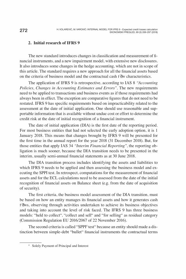
H. VOLAREVIĆ, M. VAROVIĆ: INTERNAL MODEL FOR IFRS 9 - Expected credit losses calculationEKONOMSKI PREGLED, 69 (3) 269-297 (2018)272
2. Initial research of IFRS 9
The new standard introduces changes in classiÞ cation and measurement of Þ -
nancial instruments, and a new impairment model, with extensive new disclosures.
It also introduces some changes in the hedge accounting, which are not in scope of
this article. The standard requires a new approach for all the Þ nancial assets based
on the criteria of business model and the contractual cash ß ow characteristics.
The application of IFRS 9 is retrospective, according to IAS 8 “Accounting
Policies, Changes in Accounting Estimates and Errors”. The new requirements
need to be applied to transactions and business events as if those requirements had
always been in effect. The exception are comparative Þ gures that do not need to be
restated. IFRS 9 has speciÞ c requirements based on impracticability related to the
assessment at the date of initial application. One should use reasonable and sup-
portable information that is available without undue cost or effort to determine the
credit risk at the date of initial recognition of a Þ nancial instrument.
The date of initial application (DIA) is the Þ rst date of the reporting period.
For most business entities that had not selected the early adoption option, it is 1
January 2018. This means that changes brought by IFRS 9 will be presented for
the Þ rst time in the annual report for the year 2018 (31 December 2018). But, for
those entities that apply IAS 34 “Interim Financial Reporting”, the reporting ob-
ligation is much sooner, because the DIA transition needs to be presented in the
interim, usually semi-annual Þ nancial statements as at 30 June 2018.
The DIA transition process includes identifying the assets and liabilities to
which IFRS 9 needs to be applied and then assessing the business model and ex-
ecuting the SPPI test. In retrospect, computations for the measurement of Þ nancial
assets and for the ECL calculations need to be assessed from the date of the initial
recognition of Þ nancial assets on Balance sheet (e.g. from the date of acquisition
of security).
The Þ rst criteria, the business model assessment of the DIA transition, must
be based on how an entity manages its Þ nancial assets and how it generates cash
ß ows, observing through activities undertaken to achieve its business objectives
and taking into account the level of risk faced. The IFRS 9 has three business
models: “held to collect“, “collect and sell“ and “for selling“ as residual category
(Commission Regulation EU 2016/2067 of 22 November 2016).
The second criteria is called “SPPI4 test“ because an entity should made a dis-
tinction between simple-debt “bullet“ Þ nancial instruments the contractual terms
4 Solely Payment of Principal and Interest

H. VOLAREVIĆ, M. VAROVIĆ: INTERNAL MODEL FOR IFRS 9 - Expected credit losses calculationEKONOMSKI PREGLED, 69 (3) 269-297 (2018) 273
of which entail only cash ß ows that are solely payments of principal and related
interest, and all the rest. Interest that passes SPPI test should be the compensation
for the time value of money, credit risk and cost plus proÞ t margin, consistent with
the basic lending arrangement.
According to those two criteria, an entity should classify its Þ nancial instru-
ment in one of three categories (IAS 39 used to have four categories) which include
“at amortized cost“ (AC), “at fair value through other comprehensive income“
(FVOCI) and “at fair value through proÞ t and loss“ (FVTPL). For the Þ nancial
instruments that pass the SPPI test, depending on the business model, the top
management can choose either one of the three categories. However, in case that
the SPPI test fails, the only category left is FVTPL (Commission Regulation EU
2016/2067 of 22 November 2016).
3. Implementation of the IFRS 9 impairment model
Credit risk is usually explained as the risk that a borrower may not repay a
loan (or any type of debt) so the lender may lose the principal of the loan or the
interest on the loan, or both. Credit risk is also called “a default risk“ because it
implies the Probability of Default. IFRS 9 has single impairment model for all
the Þ nancial assets, but only for those classiÞ ed as AC or FVOCI. Financial as-
sets classiÞ ed as FVTPL do not need to be impaired in this way because they are
already “marked to market“ with Þ nancial effect presented in the P&L (KPMG,
2016).
The new impairment model is forward looking which is a big change com-
pared to the old IAS 39 incurred loss model that recognized only losses that had
arisen from past events, and was criticized for resulting in too little and too late
loss provisions. Value adjustments under IAS 39 could only be triggered by the ob-
jective facts. The new IFRS 9 impairment model is oriented more towards possible
losses in future and therefore an entity should consider much more information in
determination of such expectations of future credit losses. It involves anticipatory
Expected Credit Losses model that is expected to lead to the creation of much
bigger risk provisions without fulÞ lling the objective impairment triggers of IAS
39. The new impairment model should be activated on the booking date 1 January
2018 in the transition process for the Þ nancial assets AT and FVOCI. Credit risk
at DIA should be compared with the credit risk of initial recognition in past, so
changes in credit quality can be identiÞ ed (EY, 2014).
The new ECL impairment model consists of three stages for impairment
based on changes in credit quality (credit deterioration), that are shown in Figure 1.
H. VOLAREVIĆ, M. VAROVIĆ: INTERNAL MODEL FOR IFRS 9 - Expected credit losses calculationEKONOMSKI PREGLED, 69 (3) 269-297 (2018)274
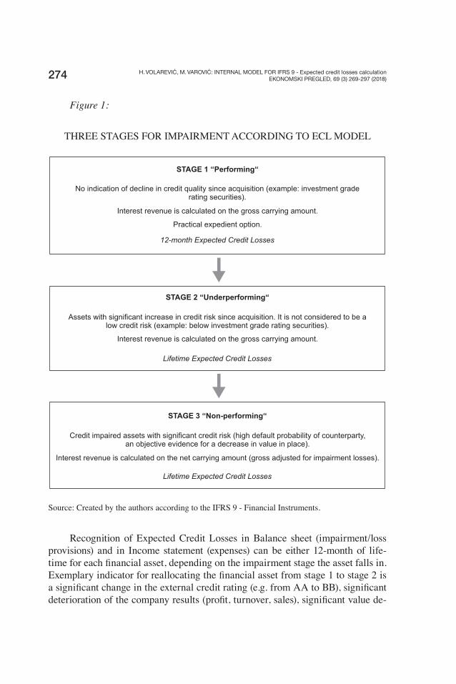
Figure 1:
THREE STAGES FOR IMPAIRMENT ACCORDING TO ECL MODEL
Source: Created by the authors according to the IFRS 9 - Financial Instruments.
Recognition of Expected Credit Losses in Balance sheet (impairment/loss
provisions) and in Income statement (expenses) can be either 12-month of life-
time for each Þ nancial asset, depending on the impairment stage the asset falls in.
Exemplary indicator for reallocating the Þ nancial asset from stage 1 to stage 2 is
a signiÞ cant change in the external credit rating (e.g. from AA to BB), signiÞ cant
deterioration of the company results (proÞ t, turnover, sales), signiÞ cant value de-
STAGE 1 “Performing“
No indication of decline in credit quality since acquisition (example: investment graderating securities).
Interest revenue is calculated on the gross carrying amount.
Practical expedient option.
12-month Expected Credit Losses
STAGE 2 “Underperforming“
Assets with significant increase in credit risk since acquisition. It is not considered to be alow credit risk (example: below investment grade rating securities).
Interest revenue is calculated on the gross carrying amount.
Lifetime Expected Credit Losses
STAGE 3 “Non-performing“
Credit impaired assets with significant credit risk (high default probability of counterparty,an objective evidence for a decrease in value in place).
Interest revenue is calculated on the net carrying amount (gross adjusted for impairment losses).
Lifetime Expected Credit Losses
?
?
H. VOLAREVIĆ, M. VAROVIĆ: INTERNAL MODEL FOR IFRS 9 - Expected credit losses calculationEKONOMSKI PREGLED, 69 (3) 269-297 (2018) 275
cline of collaterals received and days overdue for payments (usually, a 30-day de-
lay implies automatic allocation to stage 2, unless proven differently) (EBA, 2017).
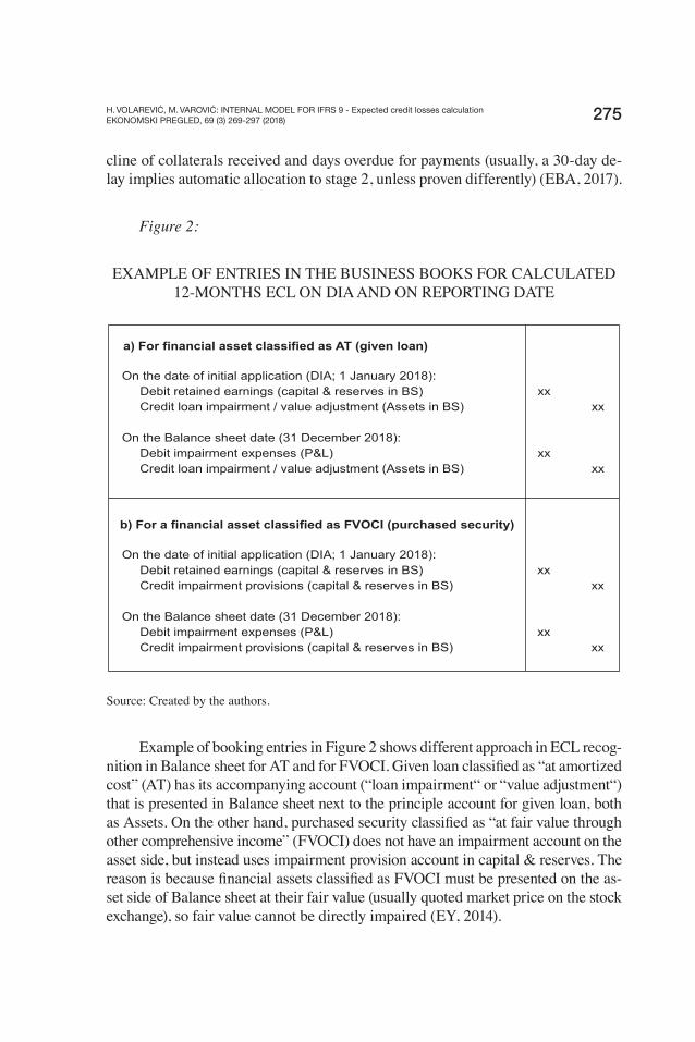
Figure 2:
EXAMPLE OF ENTRIES IN THE BUSINESS BOOKS FOR CALCULATED
12-MONTHS ECL ON DIA AND ON REPORTING DATE
Source: Created by the authors.
Example of booking entries in Figure 2 shows different approach in ECL recog-
nition in Balance sheet for AT and for FVOCI. Given loan classiÞ ed as “at amortized
cost” (AT) has its accompanying account (“loan impairment“ or “value adjustment“)
that is presented in Balance sheet next to the principle account for given loan, both
as Assets. On the other hand, purchased security classiÞ ed as “at fair value through
other comprehensive income” (FVOCI) does not have an impairment account on the
asset side, but instead uses impairment provision account in capital & reserves. The
reason is because Þ nancial assets classiÞ ed as FVOCI must be presented on the as-
set side of Balance sheet at their fair value (usually quoted market price on the stock
exchange), so fair value cannot be directly impaired (EY, 2014).
a) For financial asset classified as AT (given loan)
On the date of initial application (DIA; 1 January 2018):
Debit retained earnings (capital & reserves in BS)
Credit loan impairment / value adjustment (Assets in BS)
On the Balance sheet date (31 December 2018):
Debit impairment expenses (P&L)
Credit loan impairment / value adjustment (Assets in BS)
b) For a financial asset classified as FVOCI (purchased security)
On the date of initial application (DIA; 1 January 2018):
Debit retained earnings (capital & reserves in BS)
Credit impairment provisions (capital & reserves in BS)
On the Balance sheet date (31 December 2018):
Debit impairment expenses (P&L)
Credit impairment provisions (capital & reserves in BS)
xx
xx
xx
xx
xx
xx
xx
xx

H. VOLAREVIĆ, M. VAROVIĆ: INTERNAL MODEL FOR IFRS 9 - Expected credit losses calculationEKONOMSKI PREGLED, 69 (3) 269-297 (2018)276
One important issue to be noticed from bookings in Figure 2 is different debit
account to be used depending on the Balance sheet date. If you book ECL on date
of initial recognition, which for most entities is 1 January 2018, then the Þ nancial
effect of calculated credit losses goes to capital & reserves in Balance sheet and
charges retained earnings. This is one-time exemption for the transition from IAS
39 to IFRS 9. For all the rest reporting dates including for semi-annual report (30
June 2018) and annual report for 2018 (31 December 2018), you cannot debit re-
tained earnings, but you should always use the expense account in P&L. Thus, the
Þ nancial effects of regular ECL calculations after 1 January 2018 will decrease the
Þ nancial result for the current year, thus playing a very important role in Þ nancial
reporting and initiating interesting discussions with your external auditors (Grant
Thornton, 2016).
The new ECL model is expected to be very complex, but IFRS 9 provides
a shortcut simpliÞ cation for low credit risk Þ nancial assets in form of a practical
expedient option. Low credit risk can be justiÞ ed with high investment grade given
by the external rating agencies. Holy trinity is of course represented by the Big
Three credit rating agencies: Standard & Poor’s (S&P), Moody’s and Fitch.
The consequences of introducing IFRS 9 to your accounting would very
likely be a signiÞ cant increase in value adjustments and/or (risk) impairment
provisions that will in the short run, especially for the Þ rst year after transition,
burden the retained earnings and income statement, causing less proÞ t and less
distributable income. But, for the following years, under the assumption that the
entity would carefully manage its credit risk, a new balance will be created. The
old Þ nancial assets that will be due, matured or sold will be derecognized in the
business books and the aliquot part of the value adjustment previously recognized,
would be transferred to income side of P&L, facing new impairment expenses
that will arise from the acquisition of the new Þ nancial instruments and their ECL
calculations. The standard allows the credit risk assessment of Þ nancial assets on
a portfolio level (group / category) but it has to consist of Þ nancial instruments
with common credit risk characteristics (like instrument type, credit risk ratings,
maturity date, collateral, geographical regions) (BIS, 2015).
The biggest problem in practical implementation of the new impairment
model is the fact that IFRS 9 does not prescribe a speciÞ c measurement method
for calculating ECL model. Quite the opposite, entities are expected to develop
their internal models using reasonable and supportable information from the past
and from the future. Accountants are well aware that such a freedom looks nice
only from the outside, but when it comes to real life, a thousand questions appear,
and you have no one to ask. Actually, you can ask for help, but it is not free of
charge, far from it. It can cost you a fortune to fully implement IFRS 9 if you can-
not make it on your own.
H. VOLAREVIĆ, M. VAROVIĆ: INTERNAL MODEL FOR IFRS 9 - Expected credit losses calculationEKONOMSKI PREGLED, 69 (3) 269-297 (2018) 277
4. ECL MODEL AS A MAIN OBJECTIVE
ECL calculation model should calculate an unbiased and probability weighted
amount to be presented as impairment to book value of Þ nancial asset in Balance
sheet and it will be represent in this article as the main objective. Management can
adopt one of several methods in computing ECL. If an entity already has in place
an internal risk management model, maybe it can be updated and used for the pur-
pose of IFRS 9. But, most entities would have to start from scratch and probably
will Þ nd as very acceptable and convenient the following explicit Probability of
Default approach, shown in Figure 3.
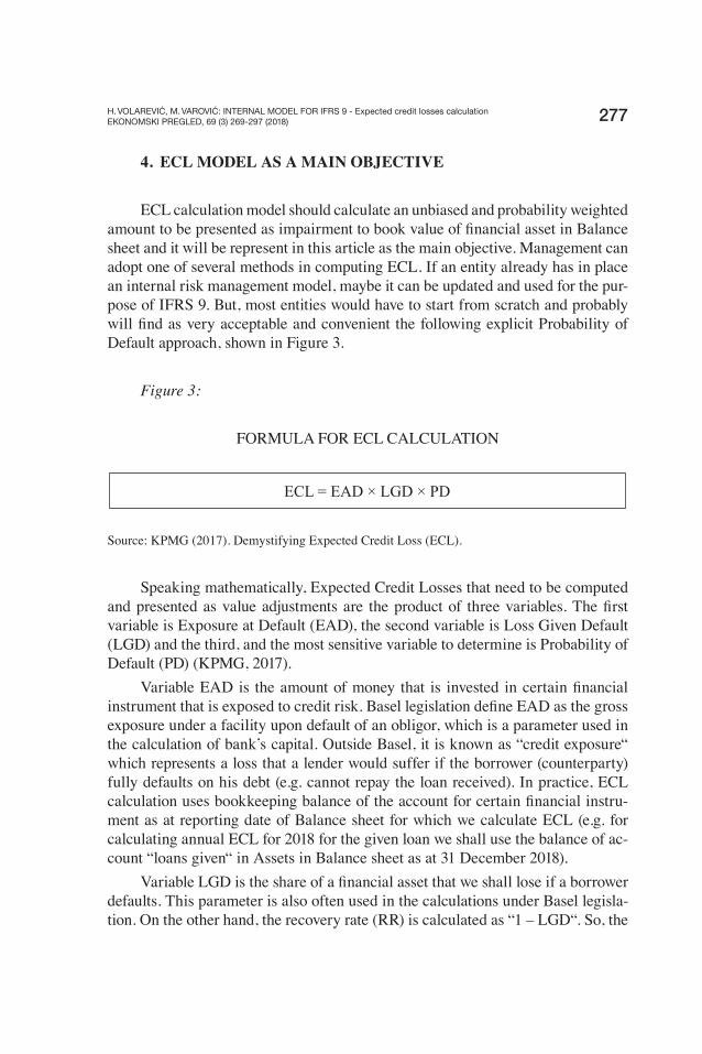
Figure 3:
FORMULA FOR ECL CALCULATION
Source: KPMG (2017). Demystifying Expected Credit Loss (ECL).
Speaking mathematically, Expected Credit Losses that need to be computed
and presented as value adjustments are the product of three variables. The Þ rst
variable is Exposure at Default (EAD), the second variable is Loss Given Default
(LGD) and the third, and the most sensitive variable to determine is Probability of
Default (PD) (KPMG, 2017).
Variable EAD is the amount of money that is invested in certain Þ nancial
instrument that is exposed to credit risk. Basel legislation deÞ ne EAD as the gross
exposure under a facility upon default of an obligor, which is a parameter used in
the calculation of bank’s capital. Outside Basel, it is known as “credit exposure“
which represents a loss that a lender would suffer if the borrower (counterparty)
fully defaults on his debt (e.g. cannot repay the loan received). In practice, ECL
calculation uses bookkeeping balance of the account for certain Þ nancial instru-
ment as at reporting date of Balance sheet for which we calculate ECL (e.g. for
calculating annual ECL for 2018 for the given loan we shall use the balance of ac-
count “loans given“ in Assets in Balance sheet as at 31 December 2018).
Variable LGD is the share of a Þ nancial asset that we shall lose if a borrower
defaults. This parameter is also often used in the calculations under Basel legisla-
tion. On the other hand, the recovery rate (RR) is calculated as “1 – LGD“. So, the
ECL = EAD × LGD × PD

H. VOLAREVIĆ, M. VAROVIĆ: INTERNAL MODEL FOR IFRS 9 - Expected credit losses calculationEKONOMSKI PREGLED, 69 (3) 269-297 (2018)278
recovery rate is the remaining share of a Þ nancial asset that we expect to recover
when a borrower defaults. For example, if we give credit of 1.000 HRK, and our
debtor starts to experience some difÞ culties, we will calculate what part of credit
we can expect debtor will repay (RR = 55%, 1,000 × 55% = 550 HRK), and what
part of credit we will lose (LGD = 1 – RR = 1 – 0.55 = 0.45 × 100 = 45%; 1,000
× 45% = 450 HRK). We must make a distinction, when calculating the value of
variable LGD, whether we have exposure with or without collateral. In previous
example, the value of LGD on our given loan is 45% (which corresponds to Basel’s
recommendation) because there is no collateral as a means of insurance and the
credit risk is bigger. Alternatively, if we receive a security as a collateral for the
given loan, then we will calculate the effective Loss Given Default that will be less
than 45% (so, in other words we expect bigger rate of return than previously 55%
because we can use collateral in case of default) (PWC, 2017).
Variable PD stands for likelihood of a default of a counterparty over an ob-
served period, usually 12 months, so an estimate of probability that a debtor will
not be able to meet its debt obligations in time or in full. PD is a key parameter
under Basel. PD calculation includes analyses of debtor’s cash ß ow adequacy in
servicing debt, operating margin, percentage of leverage used, and declining li-
quidity. There are many ways to estimate PD. It can be done by analyzing the
historical data base of actual defaults that really happened to your company or by
observing the prices of credit default swaps (CDS), bonds and options on com-
mon shares. But, the most practical way is to directly use external ratings from
S&P, Fitch and Moody’s that are based on historical data across the Þ nancial mar-
ket. Those external ratings imply a certain level of default probability and are (or
should be) objective and neutral.
For calculating ECL two types of PDs are used. For stage 1, in case of a low
credit risk, we use 12-month PD as the estimated Probability of Default occurring
within next 12 month (one year) or over the remaining maturity of the Þ nancial
instrument (e.g. receivables) that is less than 12 months. For stage 2 and 3, in case
of signiÞ cant increase of credit risk, we need to calculate lifetime PD as the es-
timated Probability of Default occurring over the remaining life of the Þ nancial
instrument, which is over 1 year (PWC, 2015).
Basel legislation favor the use of through-the-cycle (TTC) for probabilities of
default (PD), but also for LGD and EAD. Contrary to that, IFRS 9 calls for the use
of the point-in-time (PIT) estimation of PD, LGD and EAD. PIT ratings evaluate
the current situation of the counterparty by taking into account both permanent
and cyclical effect, while TTC ratings focus mostly on the permanent component
of default risk. In this article, for the purpose of developing simpliÞ ed and practi-
cal internal ECL model, we did not make a distinction between those two philo-
sophical standpoints (Topp, Perl, 2010).

H. VOLAREVIĆ, M. VAROVIĆ: INTERNAL MODEL FOR IFRS 9 - Expected credit losses calculationEKONOMSKI PREGLED, 69 (3) 269-297 (2018) 279
IFRS 9 requires the ECL calculation for all the Þ nancial instruments in
Balance sheet that are exposed to credit risk. This article will focus on the Þ nan-
cial assets on the asset side of Balance sheet. Financial assets usually include:
current accounts (a vista), term deposits placed, loans given, reverse repo deposits,
debt securities purchased, trade receivables. Cash money in our cashier’s desk is
not exposed to credit risk because it is money is in our hands; there is no counter-
party, so there is no need to calculate ECL for cash.
This is a small practical research for calculating ECL using the above for-
mula from Figure 3. Assuming we have a loan of 1,000,000 HRK given to coun-
terparty XY (credit debtor) with accrued interest on the reporting date of 5,000
HRK. Our internal risk model gives us the value of 12-month PD for counterparty
XY of 7%. Since there is no collateral received for the given loan, we can use the
standard value for LGD that is recommended by Basel legislation (45%).
12-month ECL = EAD × LGD × PD
= (1,000,000 + 5,000) × 45% × 7%
= 1,005,000 × 0.45 × 0.07
= 31,657.50 HRK
So, based on this ECL calculation, in our business books we shall debit the
impairment expense in P&L for the amount 31,657.50 HRK, and credit the value
adjustment for the loan given in Balance sheet.
4.1. DeÞ nition of EAD – Exposure at Default
Exposure at Default in the ECL calculation comes from the Accounting de-
partment, it is a bookkeeping amount of certain Þ nancial instrument from Balance
sheet for which we would like to calculate Expected Credit Losses. We will need
EAD for the initial ECL calculation on the recognition date, when the Þ nancial
instrument was acquired, for the Þ rst time. After that, we will need a bookkeeping
balance for the each reporting date for which we need to do the ECL calculation.
The amount of EAD is not just the principal of the given loan, or just the nominal
value of the security bought. EAD amount depends on the type of Þ nancial in-
strument. Below is the deÞ nition of EAD amounts for the most common types of
Þ nancial instruments that can usually be found in Assets on the Balance sheet of
business entities, on reporting date:
Loans given – EAD consists of the principle plus accrued interest up to the
reporting date.

H. VOLAREVIĆ, M. VAROVIĆ: INTERNAL MODEL FOR IFRS 9 - Expected credit losses calculationEKONOMSKI PREGLED, 69 (3) 269-297 (2018)280
Deposits placed – EAD consists of the principle plus accrued interest up
to the reporting date.
Reverse repo operations – in its accounting essence it is a deposit placed
so EAD comprises principle plus accrued interest up to the reporting date.
Debt securities purchased with discount (discounted securities) – EAD
is an amortized value plus accrued interest up to the reporting date.
Amortized value of a discounted security is its nominal value minus the
remaining (unamortized) portion of the discount.
Debt securities purchased with premium – EAD is an amortized value
plus accrued interest up to the reporting date. Amortized value is its nom-
inal value plus unamortized portion of premium.
Trade receivables – EAD amount is the nominal value of our receivables
from counterparties (customers). IFRS 9 offers possible simpliÞ cation for
ECL calculation of trade receivables (PWC, 2015).
There is no difference in calculating EAD amount for debt securities classi-
Þ ed in portfolio “at amortized cost“ (AT) in relation to debt securities in portfolio
“at fair value through other comprehensive income“ (FVOCI). Although securi-
ties in FVOCI are presented in Balance sheet at fair value, when calculating EAD
amount, we will not take into account the revaluation account (adjustment with
market value), but only the amortized value.
4.2. Calculation of LGD – Loss Given Default
Many business entities that need to apply IFRS 9 are also subject to Basel
legislation, which relates especially to Þ nancial institutions, primarily banks.
Therefore, supervisory requirements interact with Expected Credit Losses mea-
surement. Since IFRS 9 does not prescribe detailed methods of techniques for cal-
culating Expected Credit Losses, it is not forbidden to “lend“ part of the elaborated
modelling approach clearly deÞ ned in Capital Requirements Regulation – CRR
(Regulation EU No 575/2013 on prudential requirements for credit institutions
and investment Þ rms). Basel legislation (CRR) on LGD modelling and calculation
provide some ready answers, already tested in risk management in practice. In
Article 161 (CRR) it is prescribed that institutions shall use Þ xed LGD value 45%
(coefÞ cient 0.45) for non-collateralized Þ nancial instruments (for senior exposures
without eligible collateral). This Þ xed percentage is a result of historic statistical
analysis of the share the creditors in average lost when borrowers defaulted. It
means that in case of counterparty’s default, we will lose 45 out of 100 invested
(Regulation EU No 575/2013).
H. VOLAREVIĆ, M. VAROVIĆ: INTERNAL MODEL FOR IFRS 9 - Expected credit losses calculationEKONOMSKI PREGLED, 69 (3) 269-297 (2018) 281
Exposure with collateral received is much less risky. Simple calculation:
counterparty defaults with an outstanding debt of 1,000 but we can sell a security
that we received as a collateral for 850, so we lose the difference (1,000 – 850 =
150) and LGD is 15% (15/1,000 = 0.15 × 100 = 15%).
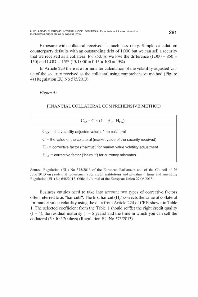
In Article 223 there is a formula for calculation of the volatility-adjusted val-
ue of the security received as the collateral using comprehensive method (Figure
4) (Regulation EU No 575/2013).
Figure 4:
FINANCIAL COLLATERAL COMPREHENSIVE METHOD
Source: Regulation (EU) No 575/2013 of the European Parliament and of the Council of 26
June 2013 on prudential requirements for credit institutions and investment Þ rms and amending
Regulation (EU) No 648/2012, OfÞ cial Journal of the European Union 27.06.2013.
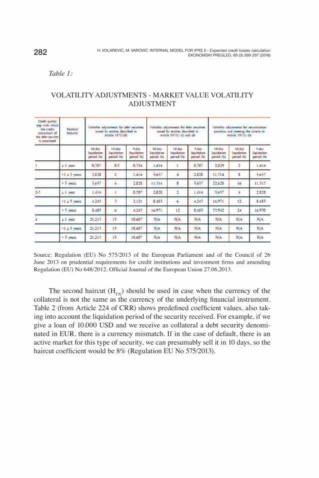
Business entities need to take into account two types of corrective factors
often referred to as “haircuts“. The Þ rst haircut (HC) corrects the value of collateral
for market value volatility using the data from Article 224 of CRR shown in Table
1. The selected coefÞ cient from the Table 1 should reß ect the right credit quality
(1 – 4), the residual maturity (1 – 5 years) and the time in which you can sell the
collateral (5 / 10 / 20 days) (Regulation EU No 575/2013).
C = C × (1 – H –H )VA C FX
CVA the volatility-adjusted value of the collateral=
C = the value of the collateral (market value of the security received)
HC = corrective factor (“haircut“) for market value volatility adjustment
HFX = corrective factor (“haircut“) for currency mismatch
H. VOLAREVIĆ, M. VAROVIĆ: INTERNAL MODEL FOR IFRS 9 - Expected credit losses calculationEKONOMSKI PREGLED, 69 (3) 269-297 (2018)282
Table 1:
VOLATILITY ADJUSTMENTS - MARKET VALUE VOLATILITY
ADJUSTMENT
Source: Regulation (EU) No 575/2013 of the European Parliament and of the Council of 26
June 2013 on prudential requirements for credit institutions and investment Þ rms and amending
Regulation (EU) No 648/2012, OfÞ cial Journal of the European Union 27.06.2013.
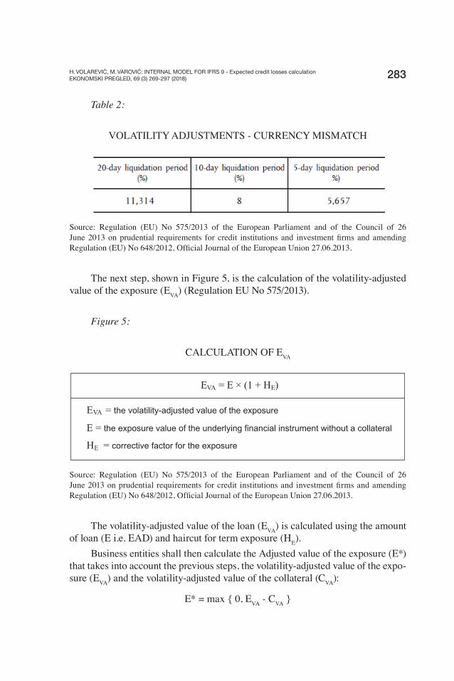
The second haircut (HFX
) should be used in case when the currency of the
collateral is not the same as the currency of the underlying Þ nancial instrument.
Table 2 (from Article 224 of CRR) shows predeÞ ned coefÞ cient values, also tak-
ing into account the liquidation period of the security received. For example, if we
give a loan of 10.000 USD and we receive as collateral a debt security denomi-
nated in EUR, there is a currency mismatch. If in the case of default, there is an
active market for this type of security, we can presumably sell it in 10 days, so the
haircut coefÞ cient would be 8% (Regulation EU No 575/2013).
H. VOLAREVIĆ, M. VAROVIĆ: INTERNAL MODEL FOR IFRS 9 - Expected credit losses calculationEKONOMSKI PREGLED, 69 (3) 269-297 (2018) 283
Table 2:
VOLATILITY ADJUSTMENTS - CURRENCY MISMATCH
Source: Regulation (EU) No 575/2013 of the European Parliament and of the Council of 26
June 2013 on prudential requirements for credit institutions and investment Þ rms and amending
Regulation (EU) No 648/2012, OfÞ cial Journal of the European Union 27.06.2013.
The next step, shown in Figure 5, is the calculation of the volatility-adjusted
value of the exposure (EVA
) (Regulation EU No 575/2013).
Figure 5:
CALCULATION OF EVA
Source: Regulation (EU) No 575/2013 of the European Parliament and of the Council of 26
June 2013 on prudential requirements for credit institutions and investment Þ rms and amending
Regulation (EU) No 648/2012, OfÞ cial Journal of the European Union 27.06.2013.
The volatility-adjusted value of the loan (EVA
) is calculated using the amount
of loan (E i.e. EAD) and haircut for term exposure (HE).
Business entities shall then calculate the Adjusted value of the exposure (E*)
that takes into account the previous steps, the volatility-adjusted value of the expo-
sure (EVA
) and the volatility-adjusted value of the collateral (CVA
):
E* = max { 0, EVA
- CVA
}
E = E × (1 + H )VA E
EVA = the volatility-adjusted value of the exposure
E = the exposure value of the underlying financial instrument without a collateral
HE = corrective factor for the exposure

H. VOLAREVIĆ, M. VAROVIĆ: INTERNAL MODEL FOR IFRS 9 - Expected credit losses calculationEKONOMSKI PREGLED, 69 (3) 269-297 (2018)284
Adjusted value of the exposure (E*) for a loan will be zero if the volatility-
adjusted value of the security received as a collateral (CVA
) is bigger than the vola-
tility-adjusted value of the exposure for a loan (EVA
). There would be no exposure
left (Regulation EU No 575/2013). Finally, entities should calculate the effective
LGD (LGD*) according to the Article 228:
LGD* = LGD × E* / E
Effective LGD (LGD*) for a loan is the multiplication of non-collateralized
LGD (45%) with uncovered (the part that remained exposed) part of a loan (E*)
in regards to the total value of a loan (total exposure). This percentage of effective
LGD* is further used in ECL calculation.
Practical research for LGD calculation: Our company has given a loan of
1,000,000 HRK and we received a German government debt security denominat-
ed in EUR with market value of 1,030,000 HRK (kuna equivalent). The maturity
of the loan is the same as the maturity of the security (2 years). There is a quite
active market for this type of security and it can be sold in 6-8 days.
E (EAD) = 1,000,000 HRK
C = 1,030,000 HRK (HRK equivalent)
HC = 15%
HFX
= 8%
HE = 0%
LGD* = ?
CVA
= C × (1 – HC – H
FX)
= 1,030,000 × (1 – 0.15 – 0.08)
= 1,030,000 × 0.77 = 793,100 HRK
EVA
= E × (1 + HE)
= 1,000,000 × (1 + 0) = 1,000,000 HRK
E* = max { 0, EVA
- CVA
}
= max { 0, 1,000,000 – 793,100 }
= max { 0, 206,900 } = 206,900 HRK
LGD* = LGD × E* / E
= 45% × 206,900 / 1,000,000
= 45% × 0.2069 = 9.31%

H. VOLAREVIĆ, M. VAROVIĆ: INTERNAL MODEL FOR IFRS 9 - Expected credit losses calculationEKONOMSKI PREGLED, 69 (3) 269-297 (2018) 285
4.3. Calculation of PD – Probability of Default
For the purpose of ECL calculation we need to determine the value of
Probability of Default (PD). Depending on the type of the underlying Þ nancial in-
strument we have to distinguish the PD of the counterparty – the debtor (to whom
you gave the loan) and PD of the issuer of the purchased debt security.
There are two ways to determine PD. The easiest way is to look it up in
transition matrices for time horizon of one year, published by external rating agen-
cies. Basic assumption is that your counterparty / issuer is a big company that is
included in the external ratings process. This is usually the case for issuers of debt
securities quoted on big stock exchanges around the world. Big external rating
agencies, for example Standard & Poor’s, publish several types of transition matri-
ces (TM), the most interesting for ECL calculations are TM for sovereign issuers,
supranational issuers, Þ nancial institutions and for corporate issuers (Standard &
Poor’s, 2017).
Table 3:
STANDARD & POOR’S TRANSITION MATRIX (TM) FROM 2016
Source: https://www.spratings.com/documents/20184/774196/2016+Annual+Global+Corporate+
Default+Study+And+Rating+Transitions.pdf/2ddcf9dd-3b82-4151-9dab-8e3fc70a7035
Table 3 shows S & P’s transition matrix for corporate issuers for 2016 issued
in April 2017, and we can see that for credit rating “BB“ default rate is 0.72%.

H. VOLAREVIĆ, M. VAROVIĆ: INTERNAL MODEL FOR IFRS 9 - Expected credit losses calculationEKONOMSKI PREGLED, 69 (3) 269-297 (2018)286
If your counterparty has external rating “BB“ then this percentage would be the
value of PD variable for ECL calculation. Optionally, PD could be adjusted if
you proportionately correct the values in column “D” with the values from col-
umn “NR” (not-rated). Additionally, if the PD value is very low i.e. close to zero,
then you should deÞ ne a minimal value for PD in your internal methodology. In
Article 163 (CRR) it is prescribed that institutions should use PD of at least 0.03%
(Regulation EU No 575/2013).
The second way, the hard way, is when your counterparty is not rated by exter-
nal rating agencies, so it has no rating, and no externally available value of PD. IFRS
9 requires that you have to set up an internal model for determining the PD value.
In literature you can Þ nd several very sophisticated and mathematically demanding
techniques to do that. The authors suggest using Analytic Hierarchy Process (AHP)
which is a multi-criteria decision making method based on mathematics and psy-
chology. AHP was developed by Thomas L. Saaty in the 1980 and it has been widely
used in various Þ elds (business, education, industry etc.). AHP structures a decision
problem, quantiÞ es its elements and links with goals, and evaluates alternative solu-
tions which in the end enables ranking of solutions. Its popularity is based primarily
on the fact that it is very similar to the way in which an individual would solve com-
plex problems by simplifying them. Psychology shows that the human brain operates
simply, that is, at the level of comparing possible pairs. It is difÞ cult to give consistent
estimates for several alternatives on multiple criteria (Saaty, 1990).
Another important reason lies in the fact that the use of this method does not
require a mathematical background. Finally, the third important reason why this
method is so popular is the possibility to use MS Excel for calculation.
In this article we will introduce an internal model for PD and therefore ECL
calculation in 9 steps which incorporates six different criteria for Þ ve selected
Croatian companies. Five companies are selected from the list of ten biggest entre-
preneurs in the Croatian business sector according to total revenues in 2016. Only
one of them (HEP group) has an external rating from Standard & Poor’s rating
agency. The Þ ve selected Croatian companies are: (1) INA group, (2) HEP group,
(3) HT group, (4) PLIVA Ltd. and (5) PLODINE Plc. Data are obtained from
their consolidated Þ nancial statements for the year 2016, available on their internet
pages and internet page of FINA (public announcement by Financial Agency).
Step 1 – Selection of Þ nancial ratios
Authors have selected the following six Þ nancial ratios from the four main
groups of Þ nancial indicators (Atrill, McLaney, 2006) that will serve as criteria
H. VOLAREVIĆ, M. VAROVIĆ: INTERNAL MODEL FOR IFRS 9 - Expected credit losses calculationEKONOMSKI PREGLED, 69 (3) 269-297 (2018) 287
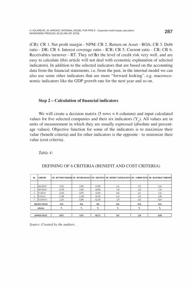
(CR): CR 1. Net proÞ t margin - NPM; CR 2. Return on Asset - ROA; CR 3. Debt
ratio - DR; CR 4. Interest coverage ratio - ICR; CR 5. Current ratio - CR; CR 6.
Receivables turnover - RT. They reß ect the level of credit risk very well, and are
easy to calculate (this article will not deal with economic explanation of selected
indicators). In addition to the selected indicators that are based on the accounting
data from the Þ nancial statements, i.e. from the past, in the internal model we can
also use some other indicators that are more “forward looking”, e.g. macroeco-
nomic indicators like the GDP growth rate for the next year and so on.
Step 2 – Calculation of Þ nancial indicators
We will create a decision matrix (5 rows × 6 columns) and input calculated
values for Þ ve selected companies and their six indicators (Yij). All values are in
units of measurement in which they are usually expressed (absolute and percent-
age values). Objective function for some of the indicators is to maximize their
value (beneÞ t criteria) and for other indicators is the opposite - to minimize their
value (cost criteria).
Table 4:
DEFINING OF 6 CRITERIA (BENEFIT AND COST CRITERIA)
Source: Created by the authors.

H. VOLAREVIĆ, M. VAROVIĆ: INTERNAL MODEL FOR IFRS 9 - Expected credit losses calculationEKONOMSKI PREGLED, 69 (3) 269-297 (2018)288
Step 3 – Calculation of six beneÞ t criteria
Next step is to deÞ ne decision matrix according to the six given criteria (Yj
for j=1, 2, 3, 4, 5, and 6). In this internal model we have 5 beneÞ t criteria (max)
and only 1 cost criterion (min), which is the debt ratio (CR3). According to that,
we will calculate the reciprocal value of the debt ratio (1/Y3). In that way, we will
create decision matrix only with beneÞ t criteria (max), all six of them.
Table 5:
CALCULATION OF 6 BENEFIT CRITERIA
Source: Created by the authors.
Step 4 – Transformation of 6 beneÞ t criteria
After we created a positively oriented decision matrix (which includes all
beneÞ t criteria) we can proceed with percentage transformation of each criterion.
This transformation includes the values of criteria between 0 and 1 according to
the following relation (Sawaragi, Nakayama, Tanino, 1985):
rij=
Yij
Yijt=1
5where is i = 1, 2, 3, 4, 5 for the companies and j = 1, 2, 3, 4, 5,
6 for criteria.
For each column i.e. value of criterion, total of values should be equal to one.

H. VOLAREVIĆ, M. VAROVIĆ: INTERNAL MODEL FOR IFRS 9 - Expected credit losses calculationEKONOMSKI PREGLED, 69 (3) 269-297 (2018) 289
Table 6:
PERCENTAGE TRANSFORMATION OF 6 BENEFIT CRITERIA
Source: Created by the authors.
Step 5 – Forming of comparison matrix
In this model criteria are ranked according to their importance (Saaty’s scale
of relative importance) as follows (Saaty, 1980). The Þ rst group of criteria (CR 1
& CR 2) includes proÞ tability ratios as the most important ratios in this model.
The second group of criteria (CR 3 & CR 4) includes solvency criteria that are less
important than the Þ rst group. Finally, the third group of criteria consists of one
criterion (CR 5) from the liquidity group and one criterion (CR 6) from the activ-
ity group which are least important in this model. Within the problem of decision
making, not all the criteria are usually equally important and the relative impor-
tance of criteria is derived from the preferences of the decision maker, i.e. authors
of the article in this case. Anyone else could group criteria differently and express
some other preferences as a decision maker.
The criteria are compared in pairs relative to how many times one is more
important than the other for achieving the set goal (by using a ratio scale). The
comparison matrix A is formed with elements aij, which represent the numerical
preference of criterion i over criterion j. This matrix is positive and the matrix ele-
ments are positive numbers. In addition, it is also true that aij = 1/a
ij for each pair
of indices (i,j). After this, it is examined whether this matrix is consistent, and if
not, the consistency index is determine. For comparison matrix A = (aij) it can be
said that it is consistent if aij = a
ik×a
kj for each (i,j,k). If the matrix is consistent,
its elements are ratios of relative importance of weights (W), and aij = W
i / W
j.
Alternatives are compared to each other in pairs for each of the criteria, assessing

H. VOLAREVIĆ, M. VAROVIĆ: INTERNAL MODEL FOR IFRS 9 - Expected credit losses calculationEKONOMSKI PREGLED, 69 (3) 269-297 (2018)290
the extent to which one of the criteria is given an advantage compared to the other.
A series of matrices is formed and used to compare alternatives for each criterion
separately, as shown in Table 7 (Saaty, 1990).
Table 7:
COMPARISON MATRIX A
Source: Created by the authors.
Step 6 – Calculation of local priorities
After deÞ ning the comparison matrix A, we should calculate local priorities,
i.e. weights of each criterion in the model (Saaty, 1990). If we divide elements
from the Þ rst column in the comparison matrix A by total sum for that column,
i.e. criterion (Table 7), we will get a value of weights for that criterion. If we repeat
that calculation for each column in the comparison matrix A, we will get the same
result for weights for all six criteria, as shown in Table 8. Finally, total value of all
weights for selected criteria in the model should be equal to one (W1 + W
2 + W
3 +
W4 + W
5 + W
6 = 1).
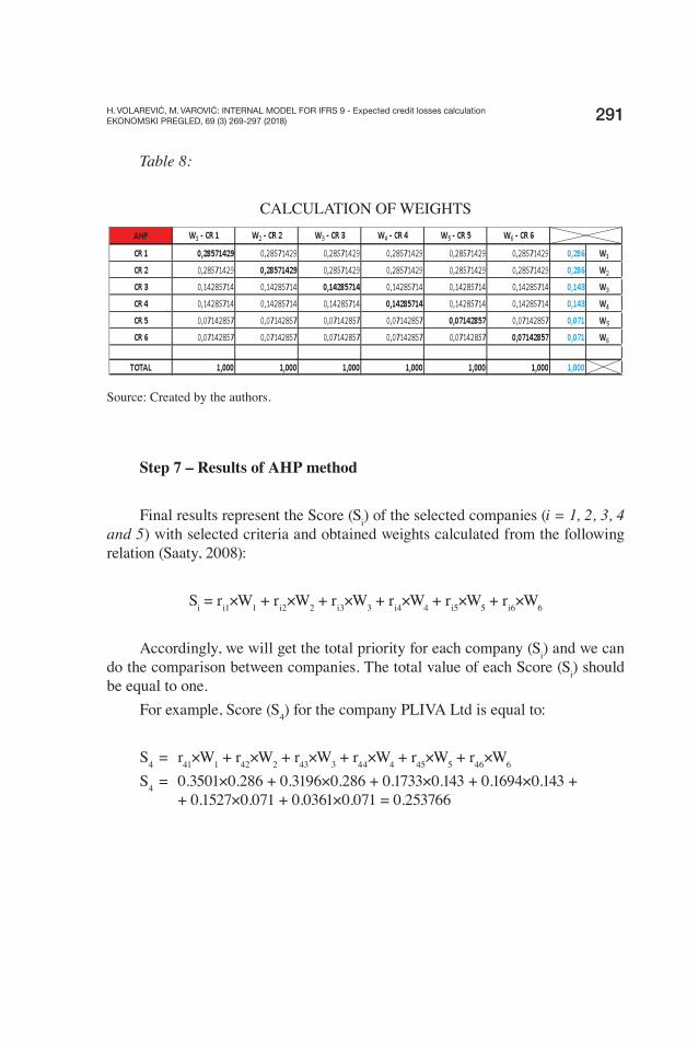
H. VOLAREVIĆ, M. VAROVIĆ: INTERNAL MODEL FOR IFRS 9 - Expected credit losses calculationEKONOMSKI PREGLED, 69 (3) 269-297 (2018) 291
Table 8:
CALCULATION OF WEIGHTS
Source: Created by the authors.
Step 7 – Results of AHP method
Final results represent the Score (Si) of the selected companies (i = 1, 2, 3, 4
and 5) with selected criteria and obtained weights calculated from the following
relation (Saaty, 2008):
Si = r
i1×W
1 + r
i2×W
2 + r
i3×W
3 + r
i4×W
4 + r
i5×W
5 + r
i6×W
6
Accordingly, we will get the total priority for each company (Si) and we can
do the comparison between companies. The total value of each Score (Si) should
be equal to one.
For example, Score (S4) for the company PLIVA Ltd is equal to:
S4 = r
41×W
1 + r
42×W
2 + r
43×W
3 + r
44×W
4 + r
45×W
5 + r
46×W
6
S4 = 0.3501×0.286 + 0.3196×0.286 + 0.1733×0.143 + 0.1694×0.143 +
+ 0.1527×0.071 + 0.0361×0.071 = 0.253766

H. VOLAREVIĆ, M. VAROVIĆ: INTERNAL MODEL FOR IFRS 9 - Expected credit losses calculationEKONOMSKI PREGLED, 69 (3) 269-297 (2018)292
Table 9:
SCORES OF AHP METHOD
Source: Created by the authors.
Step 8 – Final ranking of the companies
The Þ nal ranking of companies is shown in descending order, with the com-
pany with the highest Score being the best ranked (Zeleny, 1982). In this case, HT
group is the company with the highest Score and INA group has the lowest Score.
Table 10:
FINAL RANKING IN THE MODEL
Source: Created by the authors.

H. VOLAREVIĆ, M. VAROVIĆ: INTERNAL MODEL FOR IFRS 9 - Expected credit losses calculationEKONOMSKI PREGLED, 69 (3) 269-297 (2018) 293
Starting point in Step 8 is HEP group as the only one which has external credit
rating “BB” (Standard & Poor’s) and in transition matrix, this credit rating has the
value of PD equal to 0.72%. Using the mathematical proportion, we can get PD val-
ues for four other companies, that do not have external credit ratings of their own but
have results (Scores) according to the internal model based on AHP method.
Practical example of PD calculation for HT group:
Score (HEP) = 0.243012
Score (HT) = 0.291646
PD (HEP) = 0.72%
PD (HT) = ?
PD (HT) = (Score (HEP) / Score (HT)) × PD (HEP)
= (0.243012 / 0.291646) × 0.72%
= 0.833243 × 0.72%
= 0.599934%
Step 9 – ECL calculation
Finally, we can show a research example of ECL variable calculation which
includes EAD, LGD and PD parameters:
Our company has sold merchandise to PLODINE Plc. and has receivables
in the amount of 5,000,000 HRK. There is no collateral. PD of counterpar-
ty (PLODINE) is determined in step 8 and it equals 1.321%. We will calculate
12-month ECL which is in case of receivables the same as lifetime ECL.
EAD = 5,000,000 HRK
LGD = 45%
PD (PLODINE) = 1.321%
ECL = ?
ECL = EAD × LGD × PD
= 5,000,000 × 45% × 1.321%
= 29,722.50 HRK
Expected credit losses are 29,722.50 HRK and should be posted in P&L as the
impairment expense, and also in Balance sheet as value adjustment for the receivables.

H. VOLAREVIĆ, M. VAROVIĆ: INTERNAL MODEL FOR IFRS 9 - Expected credit losses calculationEKONOMSKI PREGLED, 69 (3) 269-297 (2018)294
5. IT support
The implementation of IFRS 9 is impossible without adequate IT support.
For bigger business entities that have their own IT departments, the cheapest solu-
tion would be to develop their own in-house IT solution (ECL-IT). The alternative,
of course, is to buy a ready software. In both cases, ECL-IT needs to be interfaced
to the accounting IT solution (ACC-IT) and to the Treasury & Risk management
IT solution (TRE-IT). Preparation and conÞ guration of ECL-IT needs to be done
by the Accounting Department in close cooperation with the Treasury and Risk
management departments. ECL needs to be calculated for each reporting date, at
least annually for the reporting date 31 December, but it is advisable to calculate
ECL monthly for the purpose of true and fair internal Þ nancial reporting.
ECL-IT will import the amounts related to Þ nancial instruments from ACC-
IT and calculate variable EAD (including the accrued interest). Risk management
and Treasury should determine and do the input of values of LGD (for collateral)
and PD for the counterparties. Having all three variables, the ECL-IT will perform
an ECL calculation. ECL-IT has to transform the ECL calculation into a posting
transaction to be exported to ACC-IT. It has to be booked analytically on the level
of each Þ nancial instrument. Each new ECL calculation has to take into account
the previous ECL calculation for the same Þ nancial instrument, so the posting
transaction in P&L should be only the difference. In case the next ECL calcula-
tion is done for a Þ nancial instrument that has been sold or matured meanwhile
(derecognition), then ECL-IT should produce a different posting transaction in
favor of revenue. In-built internal IT control should ensure that ECL-IT calculates
ECL only for “live“ Þ nancial instruments, still presented in Balance sheet. Before
the validation of these bookings, the Risk management and Treasury should car-
ry out control and make the authorization of used variables and calculated ECL.
Consequently, ECL-IT should have various groups of users having different kind
of roles (user rights).
6. Conclusion
As announced in the introductory section, this article offers a solution for
implementing the most difÞ cult part of new IFRS 9 i.e. the development of internal
model for calculation of Expected Credit Losses for Þ nancial instruments. The ar-
ticle contains both theoretical and practical instructions for deÞ ning, determining
and computing all three variables in the ECL formula: Exposure at Default (EAD),
Loss Given Default (LGD) and Probability of Default (PD).

H. VOLAREVIĆ, M. VAROVIĆ: INTERNAL MODEL FOR IFRS 9 - Expected credit losses calculationEKONOMSKI PREGLED, 69 (3) 269-297 (2018) 295
Variable EAD is an accounting amount, it is either nominal or amortized value
plus accrued interest. Determination of the LGD variable, in absence of detailed stip-
ulation in IFRS 9, is borrowed from the Basel’s Capital Requirements Regulations,
and it distinguishes whether there is collateral received or not (Regulation EU No
575/2013). The authors propose Analytic Hierarchy Process (AHP) as an appropriate
mathematical technique for calculating the third, crucial variable – PD.
The creation of such mathematical decision making problem starts with the
selection of criteria, in this case known as Þ nancial indicators (Horngren, Oliver,
2010), from basic Þ nancial statements of the selected companies (selected from
the list of the ten biggest entrepreneurs in the Croatian business sector according
to total revenues in 2016). Criteria are attributes which describe the success and
safety of the company’s business and their purpose is to provide information about
achieving a desired goal. The main objective of such multi criteria decision mak-
ing problem is to create a list of ranked companies with a speciÞ c score which is
mathematically related to the calculation of PD variable. The minimum require-
ment for the use of this model is the existence of at least one company, in the list
of the selected companies, with the deÞ ned credit rating from the external rating
agency (in this case, Standard & Poor’s). The created internal model can be solved
by MS Excel, which gives a possibility of a user friendly appliance.
It should be pointed out that the solution described is simpliÞ ed but tested in
practice and that it is compliant with all the requirements of IFRS 9. Many busi-
ness entities, including commercial banks and similar Þ nancial organizations, may
Þ nd it useful. However, they need to approach this issue in a more complex way.
LITERATURE
Atrill, P., McLaney, E. (2006). Accounting and Finance for Non-Specialists. Harlow.
Prentice Hall, 5th edition.
Bank for International Settlements, Basel Committee on Banking Supervision (2015).
Guidance on credit risk and accounting for expected credit losses, ISBN 978-92-
9197-387-3, www.bis.org
Blocher, E., J., Chen, K., H., Lin, T., W. (2002). Cost Management: A Strategic Emphasis.
New York: McGraw-Hill/Irwin.
Commission Regulation (EU) 2016/2067 of 22 November 2016 amending Regulation
(EC) No 1126/2008 adopting certain international accounting standard sin accor-
dance with Regulation (EC) No 1606/2002 of the European Parliament and of the
Council as regards International Financial Reporting Standard 9 – Annex “IFRS 9
Financial Instruments”, OfÞ cial Journal of the European Union 29.11.2016.
H. VOLAREVIĆ, M. VAROVIĆ: INTERNAL MODEL FOR IFRS 9 - Expected credit losses calculationEKONOMSKI PREGLED, 69 (3) 269-297 (2018)296
EBA, (2017). Guidelines on credit institutions credit risk management practices and ac-
counting for expected credit losses, EBA / GL / 2017 / 06, http://www.eba.europa.eu/
documents/10180/1842525/Final+Guidelines+on+Accounting+for+Expected+Credi
t+Losses+%28EBA-GL-2017-06%29.pdf
Ehrgott, M., Klamroth, K., Schwehm, Ch. (2004). An MCDM approach to portfolio opti-
mization. European Journal of Operational Research, Vol. 155, pp. 752-770.
EY (2014). Impairment of Þ nancial instruments under IFRS 9, www.ey.com
EY (2015). ClassiÞ cation of Þ nancial instruments under IFRS 9, www.ey.com
Finance Trainer International Ges.m.b.H, ALMForum (2016). “Impacts of IFRS 9 on the
accounting of Þ nancial instruments”, No. 16, September 2016, Wien.
Grant Thornton (2016). Get ready for IFRS 9 – The impairment requirements, www.grant-
thornton.global
Horngren, C., T., Oliver, M., S. (2010). Managerial Accounting. New Jersey: Upper Saddle
River, Pearson Prentice Hall.
KPMG (2016). Guide to annual Þ nancial statements: IFRS 9 – Illustrative disclosures for
banks, www.kpmg.com/ifrs
KPMG (2017). Demystifying Expected Credit Loss (ECL), https://alumni.in.kpmg.com
PWC (2015). A look at current Þ nancial reporting issues – IFRS 9: ClassiÞ cation, mea-
surement & modiÞ cations – Questions and answers, www.pwc.com
PWC (2017). IFRS 9 for banks – Illustrative disclosures, www.pwc.com
Regulation (EU) No 575/2013 of the European Parliament and of the Council of 26 June 2013
on prudential requirements for credit institutions and investment Þ rms and amending
Regulation (EU) No 648/2012, OfÞ cial Journal of the European Union 27.06.2013.
Saaty, T.L. (1980). The Analytic Hierarchy Process: Planning, Priority Setting, Resource
Allocation. New York: McGraw-Hill.
Saaty, T.L. (1990). “How to make a decision: The Analytic Hierarchy Process”. European
Journal of Operational Research, Volume 48, Issue 1, Pages 9-26, September 1990.
Saaty, T.L. (2008). “Decision making with The Analytic Hierarchy Process”. International
Journal of Services Sciences, Volume 1, Pages 83-98, January 2008.
Sawaragi, Y., Nakayama, H., Tanino, T. (1985). Theory of Multiobjective Optimization.
Orlando: Academic Press, Inc.
Spratings.com, (2016), Default, Transition, and Recovery: 2016 Annual Global Corporate
Default Study And Rating Transitions, https://www.spratings.com/documents/2018
4/774196/2016+Annual+Global+Corporate+Default+Study+And+Rating+Transitio
ns.pdf/2ddcf9dd-3b82-4151-9dab-8e3fc70a7035
Standard & Poor’s, (2017). Default, Transition and Recovery: 2016 Annual Global Corporate
Default Study and Rating Transitions, www.standardandpoors.com/ratingsdirect
Streitenberger, M., Miloš Spr i , D. (2011). „Prediktivna sposobnost Þ nancijskih pokaza-
telja u predvi anju kašnjenja u otplati kredita”. Economic Review, Volume 62, No.
07-08, Pages 383-403, September 2011.
H. VOLAREVIĆ, M. VAROVIĆ: INTERNAL MODEL FOR IFRS 9 - Expected credit losses calculationEKONOMSKI PREGLED, 69 (3) 269-297 (2018) 297
Topp, R., Perl R. (2010). “Through-the-Cycle Ratings Versus Point-in-Time Ratings and
implications of the Mapping Between Both Rating Types”. Financial Markets, Insti-
tutions & Instruments, Volume 19, Issue 1, Pages 47-61, February 2010.
Zeleny, M. (1982). Multi criteria decision-making. New York: McGraw-Hill.
INTERNI MODEL ZA MSFI 9 – KALKULACIJA O EKIVANIH
KREDITNIH GUBITAKA
Sažetak
Ovaj lanak istražuje i analizira problem implementacije me unarodnog standarda Þ nancij-
skog izvještavanja 9 (MSFI 9) koji je u primjeni od 1. sije nja 2018. godine. MSFI 9 je najrelevantni-
ji za Þ nancijske institucije, ali i za sve ostale poslovne subjekte koji imaju zna ajan udjel Þ nancijske
imovine u svojoj bilanci. Glavni cilj ovog lanka je implementacija novog modela umanjenja vri-
jednosti za Þ nancijske instrumente što se iskazuje mjerenjem o ekivanog kreditnog gubitka (ECL).
Primjena ovakvog modela je u korelaciji s kreditnim rizikom poduze a za što je potrebno utvrditi
njegove osnovne varijable kao što su to izloženost riziku nevra anja kredita (EAD), postotak mo-
gu eg gubitka (LGD) i vjerojatnost nevra anja kredita (PD). Za izra un LGD-a može se koristiti
Baselska regulativa, dok se izra un PD-a zasniva na speciÞ noj metodologiji kod koje postoje dvije
razli ite opcije. Prva varijanta nudi korištenje eksternih podataka o PD-u od strane pouzdanih rej-
ting agencija. Kada ne postoji vanjski rejting, treba razviti interni model kojim se izra unava PD. U
cilju razvoja internog modela autori lanka predlažu primjenu modela višekriterijskog odlu ivanja
temeljenog na metodi analiti kog hijerarhijskog procesa (AHP). Obrada ulaznih podataka u modelu
se bazira na podacima iz Þ nancijskih izvještaja, dok se za izra un ovakvog višekriterijskog proble-
ma koristi MS Excel. Rezultati internog modela matemati ki se povezuju s vrijednostima PD-a za
svako analizirano poduze e. Jednostavna implementacija ovog internog modela daje mu prednost u
odnosu na druge puno kompleksnije modele.
Klju ne rije i: MSFI 9, o ekivani kreditni gubici (ECL), izloženost riziku nevra anja kredita
(EAD), postotak mogu eg gubitka (LGD), vjerojatnost nevra anja kredita (PD), analiti ki hijerar-
hijski proces (AHP), interni model.