h2s dispersion model
TRANSCRIPT

AIR DISPERSION MODELING OF WELL BLOWOUT AND PIPELINE RUPTURE SCENARIOS
SALT CREEK FIELD
PREPARED FOR
HOWELL PETROLEUM CORPORATION 1201 LAKE ROBBINS DRIVE
THE WOODLANDS TEXAS 77380
PREPARED BY
5777 CENTRAL AVE SUITE 100 BOULDER COLORADO 80301
SEPTEMBER 22 2005
TABLE OF CONTENTS
1 INTRODUCTION1
2 WELL BLOWOUT SCENARIO 2
21 Input Parameters2
22 Sensitivity Analysis 3
23 Model Results3
3 HYDROGEN SULFIDE SCENARIOS 4
31 Case 1 ndash Well Blowout4
32 Case 2 ndash Well Blowout4
33 Case 3 ndash Pipeline Leak 5
34 Pasquill ndash Gifford Radius of Exposure5
4 COMPARISON OF SLAB RESULTS WITH THE CONTROLLED RELEASE DATA 7
5 PIPELINE RUPTURE - HORIZONTAL AND VERTICAL RELEASES 9
51 Horizontal Releases 9
52 Vertical Releases 9
LIST OF TABLES
Table 1 Sensitivity Analysis ndash Well Blowout Modeling Table 2 Sensitivity Analysis ndash Stability Class Table 3 Controlled Release ndash Monitor Locations Table 4 SLAB Modeling Results
LIST OF FIGURES
Figure 1 Blowout Plume Dispersion ndash High Temperature Figure 2 Blowout Plume Dispersion ndash Low Temperature Figure 3 Pasquill-Gifford Radius of Exposure ndash Blowout Case 1 Figure 4 Pasquill-Gifford Radius of Exposure ndash Blowout Case 2 Figure 5 Pasquill-Gifford Radius of Exposure ndash Pipeline Leak Case 3 Figure 6 Pipeline Leak Plume Dispersion ndash High Temperature Case 3 Figure 7 Pipeline Leak Plume Dispersion ndash Low Temperature Case 3 Figure 8 Pasquill-Gifford Radius of Exposure ndash Blowout Case 1 Figure 9 Pasquill-Gifford Radius of Exposure ndash Blowout Case 2 Figure 10 Pasquill-Gifford Radius of Exposure ndash Pipeline Leak Case 3
G1065 - Howell PetroleumModeling IIIAir Dispersion Report JR 9222005
ii
Figure 11 SLAB Model Results vs 51705 Test Release of Carbon Dioxide ndash Receptor Height of 1 Foot
Figure 12 SLAB Model Results vs 51705 Test Release of Carbon Dioxide ndash Receptor Height of 4 Feet
Figure 13 SLAB Model Results vs 51705 Zoom View Test Release of Carbon Dioxide ndash Receptor Height of 4 Feet
Figure 14 SLAB Model Output Horizontal Jet Release 10 MMSCFD 3 Inch Pipe Diameter Figure 15 SLAB Model Output Horizontal Jet Release 30 MMSCFD 6 Inch Pipe Diameter Figure 16 SLAB Model Output Horizontal Jet Release 250 MMSCFD 12 Inch Pipe Diameter Figure 17 SLAB Model Output Horizontal Jet Release 290 MMSCFD 16 Inch Pipe Diameter Figure 18 SLAB Model Output Horizontal Jet Release 10 MMSCFD 3 Inch Pipe Diameter Figure 19 SLAB Model Output Horizontal Jet Release 30 MMSCFD 6 Inch Pipe Diameter Figure 20 SLAB Model Output Horizontal Jet Release 250 MMSCFD 12 Inch Pipe Diameter Figure 21 SLAB Model Output Horizontal Jet Release 290 MMSCFD 16 Inch Pipe Diameter
G1065 - Howell PetroleumModeling IIIAir Dispersion Report JR 9222005
iii
LIST OF APPENDICES
Appendix A Carbon Dioxide Dispersion Test at 12WC2NE14 Appendix B Carbon Dioxide Dispersion Test ndash Monitoring Results
1 INTRODUCTION
Howell Petroleum Corporation (Howell) is currently installing a carbon dioxide enhanced oil recovery system also known as carbon dioxide flooding at its Salt Creek Field The flooding technique is used to increase oil production from fields that have been depleted using primary and secondary oil recovery methods Howell retained Cameron-Cole LLC to perform air dispersion modeling studies to estimate downwind carbon dioxide and hydrogen sulfide concentrations resulting from various well blowout and pipeline rupture scenarios
The Environmental Protection Agency (EPA) - approved Dense Gas Dispersion (DEGADIS) model was utilized to model vertical releases associated with the scenarios DEGADIS is a dispersion model that estimates downwind or downgradient concentrations of dense (heavier than air) gases DEGADIS is primarily used to determine distances of transit resulting in defined gas concentrations For example DEGADIS can be used to define the potential extent of migration of concentrations defined to be hazardous based on EPA risk assessment protocols or Occupational Safety and Health Administration (OSHA) exposure thresholds DEGADIS is capable of modeling finite or continuous release sources either at ground level or as a defined jet DEGADIS can also model transient scenarios where flow rates vary with time
A second EPA-approved model SLAB was employed to model horizontal releases resulting from pipeline ruptures SLAB also simulates the atmospheric dispersion of denser-than-air releases However it was developed to model horizontal jet releases in addition to vertical jet releases SLAB calculates the concentration at downwind locations by solving the conservation equations of mass momentum and energy SLAB handles release scenarios including ground level and elevated jets liquid pool evaporation and instantaneous volume sources
Modeling output was generally compared to the 10 minute Time Weighted Averages (TWA) of hydrogen sulfide (10 parts per million [ppm]) and carbon dioxide (5000 ppm) the Immediately Dangerous to Life or Health (IDLH) threshold for hydrogen sulfide (100 ppm) and the Short Term Exposure Limit (STEL) for carbon dioxide (30000 ppm)
1
2 WELL BLOWOUT SCENARIO
The DEGADIS model is accompanied by a number of various modules that can be executed in series For the purpose of modeling the release of pressurized gas for a well blowout the JETPLU module (based on the Ooms model) was used This module is intended to predict the trajectory and dilution of a denser than air jet plume which has significant upward momentum For a well blowout the release rate would be extremely fast and it was necessary to include the gasrsquo momentum in the dispersion modeling The JETPLU module outputs concentrations at ground level and at a selected level (five feet or the breathing zone was used in this case) as well as the point at which the gas cloud impacts the ground JETPLU in conjunction with a second module (DEGBRIDG) can create an input file to DEGADIS based on concentrations at the point at which the plume first contacts ground level However it was found that for all of the conditions modeled the concentration of the plume after it touched down was well below 5000 ppm carbon dioxide and thus it was not necessary to run the DEGADIS model
21 INPUT PARAMETERS
Howell supplied the expected exhaust gas parameters for a well blowout
Release Rate 16 million standard cubic feet per day (MMSCFD)
Release Temperature 0degFahrenheit (F)
Pipe Diameter 22 inches internal diameter
Duration of blowout - 36 to 48 hours
Gas composition -
963 Carbon Dioxide
07 Nitrogen
27 Methane
02 Butane
0018 Hydrogen Sulfide
The gases released under these conditions will be moving very quickly over 8000 ftsec several times the speed of sound Numerous hazards are associated with this type of release The only hazard addressed by this report is the risk associated with inhalation of these gases
For simplicity it was assumed that the release was 100 carbon dioxide At these concentrations assuming that the hydrogen sulfide disperses with the carbon dioxide the carbon dioxide concentration will be the primary inhalation concern for a well blowout The modeling runs were made using the most conservative blowout duration assuming a constant release that lasts 48 hours
2
Howell requested that the well blowout be modeled with the weather parameters held constant at worst case conditions With a high momentum release such as the one proposed here the model shows that the plume will lift into the air and then gradually drift downwind based on the influence of gravity
22 SENSITIVITY ANALYSIS
In order to ascertain worst case conditions a sensitivity analysis was performed The initial analysis showed that the worst case weather conditions were hot ambient temperatures low winds and high ambient pressures The Pasquill Stability Class sensitivity analysis (Table 1) results showed that the worst of the three cases considered was the intermediate Stability Class (D) rather than either the more stable (F) or the less stable (B) Stability Classes considered This is due to the complex interaction of Stability Class and elevated plumes Thus it was considered appropriate to determine whether the worst case Stability Class remained Class D after setting all other parameters to their final worst case settings in the model The results of this secondary sensitivity analysis which include only the effect of Pasquill Stability Class are shown in Table 2 The results show that at these conditions Stability Class D again results in the worst case scenario
23 MODEL RESULTS
Despite these conservative assumptions in all of the runs at all of the weather conditions tested the maximum concentration of carbon dioxide at ground level and in the breathing zone (five feet) was 192 ppm well below the lowest regulatory threshold of 5000 ppm Hydrogen sulfide concentrations are well below 1 ppm under all conditions and are also not expected to be of concern
It should be noted that this model does not evaluate conditions in the immediate vicinity of the blowout (generally a radius of about 100 feet from the center of the source) for these input parameters However if there is a blowout people within the immediate vicinity of the blowout will face considerable hazards in addition to any inhalation hazard and once the blowout has occurred it is recommended that access in the immediate vicinity of the site be limited to those with appropriate respiratory apparatus and other appropriate safety gear
3
3 HYDROGEN SULFIDE SCENARIOS
DEGADIS was utilized to model four scenarios depicting hydrogen sulfide releases at Howellrsquos Salt Creek Field The radii of exposure based on the Pasquill ndash Gifford equation for each of the scenarios was also calculated
Three of the scenarios (Cases 1 2 and 3) were based on the worst case conditions as determined by the Monte Carlo analyses contained in the Air Dispersion Modeling in Support of Risk Analysis Report (Cameron-Cole April 2005) The Monte Carlo simulations utilized actual weather conditions and varied the input parameters to determine the effects on the output from the DEGADIS model It was determined that minimum wind speed a Wind Stability Class of D and high ambient temperatures created the worst case conditions (highest downwind hydrogen sulfide concentrations) The fourth scenario utilized Case 3 input parameters except for the high ambient temperature A lower ambient temperature was used to evaluate lesser downwind concentrations
The details of each scenario and the associated output presented below
31 CASE 1 ndash WELL BLOWOUT
Wind speed - approximately 1 mile per hour (mph) Stability Class - B D and F Ambient temperature - 100oF Atmospheric pressure - 087 atmosphere (atm) Relative humidity - 56 Gas flow rate - 16 mmscfd Hydrogen sulfide concentration - 180 ppm Diameter - 2 78 inch tubing
Results - no breathing zone hydrogen sulfide concentrations greater than or equal to 10 ppm
32 CASE 2 ndash WELL BLOWOUT
Wind speed - approximately 1 mph Stability Class - B D and F Ambient temperature - 100oF Atmospheric pressure - 087 atm Relative humidity - 56 Gas flow rate - 16 mmscfd
4
Hydrogen sulfide concentration - 450 ppm Diameter - 2 78 inch tubing 5 inch casing and 8 58 inch casing
Results - no breathing zone hydrogen sulfide concentrations greater than or equal to 10 ppm
33 CASE 3 ndash PIPELINE LEAK
Wind speed - approximately 1 mph Stability Class - B D and F Ambient temperature - 100oF and 32oF Atmospheric pressure - 087 atm Relative humidity - 56 Gas flow rate - 25 mmscfd Hydrogen sulfide concentration - 22000 ppm Diameter ndash 4 inch pipe
Results - at 100oF hydrogen sulfide concentrations in excess of 10 and 100 ppm were predicted (Figure 1) Hydrogen sulfide concentrations in excess of 10 ppm were also predicted with an ambient temperature of 32oF (Figure 2) Because of plume rise due to momentum and temperature downwind breathing zone concentrations were only predicted to occur once the plume settled to the ground
34 PASQUILL ndash GIFFORD RADIUS OF EXPOSURE
The more conservative Pasquill ndash Gifford Radius of Exposure calculation was also utilized to estimate the downwind distance the 100 and 500 ppm hydrogen sulfide plumes would drift before dissipating Case 1 input parameters produced 100 and 500 ppm radii of exposure of 195 and 89 feet respectively (Figure 3) Case 2 input parameters yielded 100 and 500 ppm radii of exposure of 347 feet and 158 feet respectively (Figure 4) Finally Case 3 calculations determined the 100 and 500 ppm radii of exposure would be 1237 and 565 feet respectively (Figure 5) The Pasquill ndash Gifford calculation does not allow for the input of ambient temperature therefore only three scenarios were calculated
Hydrogen sulfide concentration results from the DEGADIS model and the Pasquill ndash Gifford Radius of Exposure calculation were plotted on a topographic map of the Salt Creek Field Rather than plot the data based on specific wind directions a circular concentration field was used to illustrate the potential hydrogen sulfide concentrations regardless of wind direction The DEGADIS model did not predict hydrogen sulfide concentrations greater than or equal to 10 ppm would result from Case 1 or Case 2 input data Case 3 high temperature input data yielded a narrow band (six to 13 feet) of 10 and 100 ppm concentrations (Figure 6) 270 feet from the source Case 3 low temperature input data resulted in a 10 ppm concentration band approximately 200 feet wide (Figure 7) 550 feet from the source
5
The Pasquill ndash Gifford Radius of Exposure calculation does not take into account plume rise So the 100 and 500 ppm concentration fields are assumed to extend uniformly from the source to the downwind limits of exposure Cases 1 2 and 3 radii of exposure are presented on Figures 8 9 and 10 respectively
6
4 COMPARISON OF SLAB RESULTS WITH THE CONTROLLED RELEASE DATA
On May 17 2005 carbon dioxide was released from a wellhead at the 12WC2NE14 location in order to validate and field test the dispersion modeling The controlled release commenced at 500 am and continued for 30 minutes The flow rate was held constant at 80 MMSCFD while the release pressure was maintained at 1000 pounds per square inch (psi) Additional details on the experimental procedures and equipment are included in Appendix A
Weather conditions were estimated based on data from Casper Wyoming as recorded on the website wwwwundergroundcom Casper weather conditions at 453 am were as follows
Temperature 601deg F
Humidity 42
Wind Speed 69 mph
Wind Direction SE
Based on the time of day and the wind speed the Pasquill Stability Class was estimated to be C or moderately unstable
Eight carbon dioxide monitors were installed at locations specified with a bearing (degrees off north) and a distance from the source Four of the monitors were placed one foot off of the ground and four were placed in the breathing zone four feet off the ground The eight locations are presented in Table 3
Monitoring results are included in Appendix B Monitoring results prior to the start of the test suggest that background levels at the monitoring locations are about 600 ppm although measured values range from 556 ppm (Location 5) to 806 ppm (Location 6)
The SLAB model was run using a horizontal release rate of 8 MMSCFD (49 kilograms per second [kgs] of carbon dioxide) exiting through a 2 - inch diameter pipe The model results are plotted in Figures 11 through 13 The monitoring data recorded 15 minutes after the start of the controlled release are included on the figures
Generally the monitoring results from Locations 3 5 and 8 are close to background levels throughout the controlled release This is not surprising considering they are west or north of the source The pressurized plume was being released directly east However all three sites have occasional hits of higher carbon dioxide levels presumably due to shifting winds The SLAB model predicts that the plume will move due east from the source and that there will be no impacts to the north south and west of the source
7
Monitoring Location 1 showed carbon dioxide concentrations ranging from about 600 ppm to a high of over 6000 ppm after the monitoring location is first impacted about 10 minutes into the controlled release In comparison the model predicts concentrations would be about 20000 ppm at this location
Monitoring Location 2 showed a similar but slightly lower concentration range Measured carbon dioxide concentrations ranged from background (approximately 600 ppm) to a high near 5800 ppm This was in good agreement with the model which predicted a concentration of about 3000 ppm
Monitoring Locations 4 6 and 7 were within one foot of the surface and showed considerably higher concentrations Location 4 generally showed concentrations that varied between 9000 and 13000 ppm The modeled concentration was about 5000 ppm Over the course of the release period the concentration at Location 6 remained about 8000 ppm In comparison the modeled concentration was about 1000 ppm Location 7 concentrations varied widely from about 8000 ppm up to a maximum of almost 14000 ppm In comparison the modeled concentration was only about 300 ppm
The modeled concentrations varied above and below although within an order of magnitude of the measured concentrations The only exception was Location 7 for which the monitored concentrations were about 40 times higher than the modeled concentrations Disparities may be attributable to shifting winds or more likely the variable topography of the site Neither DEGADIS nor SLAB were designed to allow for specific topographical input data Both models use very basic terrain factors which can lead to skewed results
8
5 PIPELINE RUPTURE - HORIZONTAL AND VERTICAL RELEASES
Thirty-two different scenarios were modeled These included both a horizontal and a vertical release four different release rates carbon dioxide and hydrogen sulfide components and receptors located at ground level (the worst case for heavier than air gases) and at four feet (generally considered the breathing zone) The results are included in Table 4 and Figures 14 through 21 Horizontal jet releases were modeled using SLAB and vertical jet releases were modeled using the DEGADIS model
All runs were made at F stability and a wind speed of 1 meter per second These are considered extremely stable conditions at which dispersion is minimized This will result in the highest maximum concentrations for horizontal releases
Hydrogen sulfide concentrations were assumed to be 322 ppm in the released gas Since neither the SLAB model nor the DEGADIS model have the capabilities to predict emissions of secondary constituents it was assumed that hydrogen sulfide dispersed with the carbon dioxide and their relative concentrations remained constant Thus the 30000 ppm carbon dioxide (STEL) contour coincides with the 10 ppm hydrogen sulfide contour (10 minute TWA) and the 300000 ppm carbon dioxide contour approximates the 100 ppm hydrogen sulfide (IDLH) contour
51 HORIZONTAL RELEASES
The results of the horizontal release modeling show that the scenario release rates could result in carbon dioxide impacts exceeding 30000 ppm (STEL) 300 feet from the source and 5000 ppm (10 minute TWA) 4100 feet from the source Modeled hydrogen sulfide concentrations exceeded 10 ppm (10 minute TWA) approximately 300 feet from the source Hydrogen sulfide concentrations are not predicted to exceed 100 ppm (IDLH) in the breathing zone However hydrogen sulfide concentrations are predicted to exceed 100 ppm (IDLH) at ground level but only within the first 13 or 14 feet of the source
52 VERTICAL RELEASES
The plumes resulting from vertical jet release scenarios are predicted to dissipate before settling to the ground Concentrations exceeding 5000 ppm carbon dioxide (10 minute TWA) and 10 ppm hydrogen sulfide (10 minute TWA) are not predicted to occur in the breathing zone or at ground level
9
TABLES
Table 1
Sensitivity Analysis - Well Blowout Modeling Howell Petroleum
Salt Creek Field Wyoming
Max Concentration Distance to Max
Concentration Increase over Baseline
Max Concentration Max Concentration Distance to Max
Concentration Increase over Baseline
Max Concentration Windspeed (mph) 3 1 718 9000 37 668 1022 39
6 49 65790 -07 41 99940 -07 Elevation at which Windspeed is Measured (meters)
10
Surface Roughness (meters)
02
B 303 1602 10 247 8551 08 D 620 46520 30 503 57130 27
Monin-Obukhov Calculated 2441 55 77980 -06 49 96790 -06 2802 104 46520 -03 90 57130 -03 087 168 31130 01 147 37920 01 079 141 37830 -01 125 45520 -01
Relative Humidity () 56 Abs Humidity Calculated Ambient Air Density Calculated Gas Temp (K) 255 Flow Rate (kgs) 116 Source Radius (m) 00558 Source Elevation (m) 04 a
Carbon Dioxide Concentration Baseline 154 34330 00 136 41460 00
Ambient Pressure (atm) 083
Pasquill Stability Class F
Ambient Temp (K) 3108
Breathing Zone (15 m above ground) Ground Level Change from Baseline
Parameters Baseline Tested Values
a Minimum allowed by model
Table 2
Sensitivity Analysis - Stability Class Howell Petroleum
Salt Creek Field Wyoming
Change from Baseline Breathing Zone (15 m above ground) Ground Level
Increase over Max Concentration Distance to Max Increase over Baseline Max Concentration Distance to Max Baseline Max
Parameters Baseline Tested Values (ppm) Concentration Max Concentration (ppm) Concentration Concentration Windspeed (mph) 1 Elevation at which 10 Surface Roughness 02 (meters) Pasquill Stability Class D B 1341 1124 -08 1128 1330 -09
F 718 9003 -06 668 9716 -06 Monin-Obukhov Calculated Ambient Temp (K) 3108 Ambient Pressure (atm) 087 Relative Humidity () 56 Abs Humidity Calculated Ambient Air Density Calculated Gas Temp (K) 255 Flow Rate (kgs) 116 Source Radius (m) 00558 Source Elevation (m) 04 a
Baseline Worst Case (Carbon Dioxide)
D D 1924 1370 00 1815 1454 00
Hydrogen Sulfide 0035 0033 Concentration
a Minimum allowed by model
Table 3
Controlled Release Monitor Locations
Location Distance From Ground (feet)
Distance From Source (feet)
Bearing From Source
1 4 53 64deg 2 4 110 122deg 3 4 59 210deg 4 1 206 89deg 5 1 146 187deg 6 1 450 98deg 7 1 400 76deg 8 4 103 360deg
Notes
Bearing From Source = degrees off North
Table 4
SLAB Modeling Results Pipeline Rupture
Horizontal Release
Receptor Height (feet)
4
Source Release Rate (MMSCFD)
10
Pipe Diameter (inches)
3
Maximum Distance From Source at which CO2
Concentration Exceeds 5000 ppm
(feet)
905
Maximum Distance From Source at which H2S
Concentration Exceeds 100 ppm
(feet)
NA
Maximum Distance From Source at which CO2
Concentration Exceeds 30000 ppm and H2S
Exceeds 10 ppm (feet)
148 4 30 6 1889 NA 260 4 250 12 4047 NA 268 4 290 16 4049 NA 263
Ground level 10 3 1018 14 192 Ground level 30 6 1982 13 293 Ground level 250 12 4087 13 270 Ground level 290 16 4089 13 266
Notes Maximum occurs along centerline of plume in the direction of the release
F Stability Windspeed = 1 metersecond
FIGURES
APPENDIX A
Carbon Dioxide Dispersion Test at 12WC2NE14
CO2 dispersion Test at 12WC2NE14
The purpose of this dispersion test is to validate and field test our dispersion modeling The test conditions need to be worst case scenario calm day low lying area (draw) and a high volume release (relatively speaking) (8MM) The test will be performed early morning (between 5 and 6 am) as to not affect field personnel The well will be WAGrsquod 24hrs prior to the test to allow any water in the system to be cleared If water isnrsquot cleared from the system hydrates or ice may form Below is the procedure for performing the test
bull Set RTUrsquos (8) to record dispersion data (CO2 concentration in PPM) o Calibrate and program RTUrsquos to gather data once per second - Allan
bull Stroke 12NE14 choke to the closed position and leave RTU in local bull Shut well head gate valve
o Using the 1rdquo bleeder located on the flow ldquoTrdquo bleed off the pressure between the choke and the well head gate
bull Make up hard line and fittings from well head to ~ 60rsquo from well head running to the east ndash SEE HAND SKETCH
o Fittings 2 ndash 90ordm swivels with 1502 hammer unions 3 ndash jts of 2rdquo XH hard line with 1502 hammer unions 1- bean choke with 1rdquo bean 1 ndash 2 38rdquo perforated sub
o Make up On the 2rdquo full port wire line valve thread in a 2rdquo XH nipple with a 1502
wing half Install a 2rdquo 90ordm swivel Install a short section (~10rsquo) of 2rdquo XH hard line Install a 2rdquo 90ordm swivel Install two (2) twenty (20) foot sections of hard line
bull Hard line will be installed on top of three (3) cement blocks and chainboomered down
bull There should be one block located on the back side of the ground level 90ordm swivel
Install the bean choke Install a 2rdquo X 2 38rdquo HP swage Install a 2 38rdquo perforated sub open ended
bull Set up well (12NE14) RTU for test o Capture rate and pressure every 30 sec ndash 1 min o Set well head set point to 1000 psi o Set rate over ride to 8MM
bull Start the eight (8) RTUrsquos gathering data bull Open the 2rdquo full port wire line entry valve bull Notify affected personnel that the test is about to commence - DEM
o BJV will be monitoring the test from the office in case the test needs shut down bull Put RTU in auto and clear the area
o Monitor from a distance preferably cross wind and up hill o Stay in contact with BJV in the office monitoring CASE
If for any reason the test needs shut down BJV will do so using the CASE host
bull Reasons can include but are not limited to o Hard line plugging from the formation of dry ice o The hard line starts to rise off of the ground o The hard line starts to move from side to side front to back o Leaking fittings o Completion of the test
bull Duration of the test will be twenty (20) to thirty (30) minutes o CAUTION
H2S and CO2 gas will be present Extreme cold temperatures will be present Dry Ice may form High pressures will be present
bull Notify affected personnel of the completion of the test ndash DEM bull BJV will change the set points from CASE and notify when the well status indicates the
choke is closed bull Once the well is shut in
o Put RTU in local o Close the 2rdquo FP WL entry valve o Break all fittings apart o Open the well head gate valve o Reset the well RTU to normal injection control set points o Put the well RTU in auto o Gather all data points from the eight (8) RTU
Put in excel format bull Attachments
o Hand Sketch o Map of 12NE14 with approximate RTU locations o Map with out 12NE14 but with exact RTU location
APPENDIX B
Carbon Dioxide Dispersion Test ndash Monitoring Results
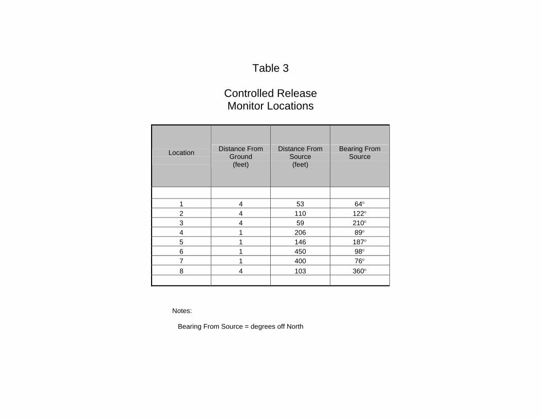

APPENDIX B
Carbon Dioxide Dispersion Test ndash Monitoring Results
