hal.inria.fr · hal id: hal-01184251 submitted on 13 jan 2016 hal is a multi-disciplinary open...

HAL Id: hal-01184251https://hal.inria.fr/hal-01184251

Submitted on 13 Jan 2016

HAL is a multi-disciplinary open accessarchive for the deposit and dissemination of sci-entific research documents, whether they are pub-lished or not. The documents may come fromteaching and research institutions in France orabroad, or from public or private research centers.

L’archive ouverte pluridisciplinaire HAL, estdestinée au dépôt et à la diffusion de documentsscientifiques de niveau recherche, publiés ou non,émanant des établissements d’enseignement et derecherche français ou étrangers, des laboratoirespublics ou privés.

Non-conforming Galerkin finite element methods forlocal absorbing boundary conditions of higher order

Kersten Schmidt, Julien Diaz, Christian Heier

To cite this version:Kersten Schmidt, Julien Diaz, Christian Heier. Non-conforming Galerkin finite element methods forlocal absorbing boundary conditions of higher order. Computers and Mathematics with Applications,Elsevier, 2015, 70 (9), pp. 2252–2269. 10.1016/j.camwa.2015.08.034. hal-01184251

https://hal.inria.fr/hal-01184251

https://hal.archives-ouvertes.fr

Computers and Mathematics with Applications 70 (2015) 2252–2269

Contents lists available at ScienceDirect

Computers and Mathematics with Applications

journal homepage: www.elsevier.com/locate/camwa

Non-conforming Galerkin finite element methods for localabsorbing boundary conditions of higher orderKersten Schmidt a,∗, Julien Diaz b,c, Christian Heier aa Research Center MATHEON, TU Berlin, 10623 Berlin, Germanyb Laboratoire de Mathématiques et de leurs Applications, UMR5142, Université de Pau et des Pays de l’Adour, 64013 Pau, Francec Project MAGIQUE-3D, INRIA Bordeaux-Sud-Ouest, 64013 Pau, France

a r t i c l e i n f o

Article history:Received 29 November 2014Received in revised form 4 August 2015Accepted 18 August 2015Available online 26 September 2015

Keywords:Interior penalty Galerkin finite elementmethods

Local absorbing boundary conditions

a b s t r a c t

A new non-conforming finite element discretization methodology for second order ellipticpartial differential equations involving higher order local absorbing boundary conditions in2D and 3D is proposed. The novelty of the approach lies in the application of C0-continuousfinite element spaces, which is the standard discretization of second order operators, tothe discretization of boundary differential operators of order four and higher. For each ofthese boundary operators, additional terms appear on the boundary nodes in 2D and onthe boundary edges in 3D, similarly to interior penalty discontinuous Galerkin methods,which leads to a stable and consistent formulation. In this way, no auxiliary variables onthe boundary have to be introduced and trial and test functions of higher smoothness alongthe boundary are not required. As a consequence, themethod leads to lower computationalcosts for discretizations with higher order elements and is easily integrated in high-orderfinite element libraries. A priori h-convergence error estimates show that the methoddoes not reduce the order of convergence compared to usual Dirichlet, Neumann or Robinboundary conditions if the polynomial degree on the boundary is increased simultaneously.A series of numerical experiments illustrates the utility of the method and validates thetheoretical convergence results.

© 2015 Elsevier Ltd. All rights reserved.

1. Introduction

Modelling of complex systems in science and engineering, for example in electromagnetics, mechanics, acoustics orquantum mechanics, often require the problem to be reduced to a domain of interest and conditions on its boundary aredescribed to incorporate the state of the system exterior to this computational domain. Very often local absorbing andimpedance boundary conditions [1–3] are used, where Dirichlet, Neumann and Robin boundary conditions are the mostprominent examples. To achieve higher accuracy, local absorbing boundary conditions of higher order are derived, whichpossess higher tangential derivatives that are even of order four and higher. In this paper, solutions of second order partialdifferential equations (PDEs) in a connected Lipschitz domain Ω ∈ Rd, d = 2, 3 subject to local absorbing boundaryconditions (ABCs) on a closed subset Γ of the boundary ∂Ω are considered. As prominent exponent are the symmetric local

∗ Corresponding author.E-mail address: [email protected] (K. Schmidt).

http://dx.doi.org/10.1016/j.camwa.2015.08.0340898-1221/© 2015 Elsevier Ltd. All rights reserved.

http://dx.doi.org/10.1016/j.camwa.2015.08.034

http://www.elsevier.com/locate/camwa

http://www.elsevier.com/locate/camwa

http://crossmark.crossref.org/dialog/?doi=10.1016/j.camwa.2015.08.034&domain=pdf

mailto:[email protected]

http://dx.doi.org/10.1016/j.camwa.2015.08.034

K. Schmidt et al. / Computers and Mathematics with Applications 70 (2015) 2252–2269 2253

absorbing boundary conditions (see [4, Eq. 3.14] and [5]), which are given for d = 2 as

∂νu +

Jj=0

(−1)j∂ jΓ (αj∂

jΓ u) = g, (1)

where ∂ν and ∂Γ denote the normal and tangential derivatives on Γ , ∂ν := ν · ∇ , ∂Γ = τ · ∇ , ν is the outer unit normalvector on Γ and τ the unit tangential vector. Furthermore, αj, j = 0, . . . , J and g are smooth enough functions on Γ , andJ ∈ N0 ∪ −1 is the order of highest (second) derivatives. Local ABCs for J = −1, 0 are well-known as Neumann (J = −1)and Robin boundary conditions (J = 0) and for J = 1 possibly less known as Wentzell boundary conditions (see [6] andthe references therein). The discretization of second order PDEs with local ABCs by the usual C0-continuous finite elementmethods (FEM) has been so far restricted to these three cases (see, e.g., [7] for Wentzell’s conditions). For local ABCs of anyorder J finite element methods with C (J−1)-continuous basis functions (at least) along Γ [8,4] or with auxiliary unknowns[9,10] for each ∂2

Γ u, ∂4Γ u up to ∂

2(J−1)Γ u leading to a mixed system have been proposed. Even so, local ABCs with derivatives

higher than two have rarely been used so far.In this article, C0-continuous finite element methods were proposed for local symmetric ABCs of any order J , for both

d = 2, 3, and are analysed when they are applied to the Helmholtz equation. These finite element methods are inspired byinterior penalty discontinuous Galerkinmethods [11] and exhibit additional terms on boundary nodes for d = 2 or boundaryedges for d = 3. A similar approach was introduced by Brenner and Sung [12] for fourth order partial differential equations.Moreover, additional terms are introduced in the formulation if also tangential derivatives of odd orders are present, as thisis the case for several impedance boundary conditions. Eventually, for d = 3 even more general boundary conditions withhigher tangential derivatives applied to the Neumann trace are considered.

The article is organized as follows. In Section 2 several examples of local ABCs are given and corresponding variationalformulations are introduced. Then, interior penalty formulations in two dimensions are introduced in Section 3 and in threedimensions in Section 4. The numerical analysis of the numerical method proposed in the article is presented for the caseof local symmetric ABCs in two dimensions in Section 5. Finally, in Section 6 the proven theoretical convergence results arevalidated by a series of numerical experiments.

2. Local absorbing boundary conditions

Local ABCs are stated for example on artificial boundaries of truncated, originally infinite domains to approximate radi-ation or decay conditions [13,2]. Then, the functions αj in (1) correspond to PDEs outside Ω and a better approximation isobtained by moving the artificial boundary further to infinity or by adding further terms, i.e., increasing J .

If a possibly bounded subdomain correspond to a highly conducting body in electromagnetics, the fields can be com-puted approximately by a formulation in the exterior of the conductor with so-called surface or generalized impedanceboundary conditions [14,1,3] on the conductor surface. While introduced first by Rytov [15] and Leontovich [16], in recentyears impedance boundary conditions of higher orders are proposed [17,18]. Similar impedance boundary conditions werederived for thin dielectric coatings on perfect conducting bodies [19–22] or for viscosity boundary layers in acoustics [23].Furthermore, impedance transmission conditionsmay be used to approximate the behaviour of thin layers (see [24] and thereferences therein) or even microstructured layers [25]. In this case they relate jumps and means of Dirichlet and Neumanntraces on the mid-surface of the layer.

The derivation of these local ABCs is often performed by asymptotic expansion techniques or by a truncation of Fourierseries, where, at least for the rigorous error estimates, the boundary Γ and the functions αj are assumed to be smooth. Thelocal ABCs may also be applied for piecewise smooth boundaries Γ , e.g., domains with corners, or for piecewise smoothfunctions αj which may have jumps. In this case the higher surface derivatives ∂

jΓ αj∂

jΓ are not necessary weak derivatives

on the whole boundary Γ and additional conditions on the corners are needed [26]. To knowledge of the authors of thisarticle, those corner conditions have not beenmathematically analysed so far and this analysis is restricted to Γ ∈ C∞ withring topology and αj ∈ C∞, j = 0, . . . , J .

With these assumptions, the weak form of (1), after j-time integration by parts of the jth term along Γ is, with v smoothenough, given by

Γ

∂νuv +

Jj=0

αj∂jΓ u ∂

jΓ v dσ(x) =

Γ

gv dσ(x). (2)

If the local ABCs are used in combination with the Helmholtz equation with homogeneous Neumann boundary conditionson ∂Ω\Γ the corresponding variational formulation reads: Seek uJ ∈ VJ := v ∈ H1(Ω) : v|Γ ∈ H J(Γ ) such that

aJ(uJ , v) :=

Ω

∇uJ · ∇v − κ2uJv

dx +

Jj=0

Γ

αj∂jΓ uJ ∂

jΓ v dσ(x) =

fJ , v

∀ v ∈ VJ , (3)

where fJ corresponds to source terms in the domain Ω or on the boundary Γ and the wave number κ ∈ L∞(Ω).

2254 K. Schmidt et al. / Computers and Mathematics with Applications 70 (2015) 2252–2269

If only second derivatives are present in (1) and so only first derivatives in (3), i.e., for the Neumann, Robin andWentzellconditions, a numerical realizationwith usual piecewise continuous finite elementmethods is straightforward. For J ≥ 2, theusual finite element spaces are not contained anymore in the natural space VJ of the continuous formulation. For those high-order conditions, finite elements methods with C0-continuous basis functions will be introduced in the following section.

3. Interior penalty finite element formulation in 2D

For the derivation of the interior penalty formulation, the following regularity result is needed.

Lemma 3.1. Let uJ ∈ VJ be solution of (3)with infx∈Γ |αJ | > 0 and κ ∈ C∞(ΩΓ ) in some neighbourhood ΩΓ ⊂ Ω of Γ . Then,uJ ∈ C∞(Γ ).

Proof. The proof is a simple generalization of the proof of Lemma 2.8 in [5] from circular to C∞ boundary Γ , from constantsαj to αj ∈ C∞, and from constants κ in some neighbourhood of Γ to C∞-functions in such a neighbourhood.

3.1. Definition of the C0-continuous finite element spaces

The presented non-conforming finite elementmethod is based on ameshMh of the computational domainΩ (see Fig. 1)consisting of possibly curved triangles Th and curved quadrilaterals Qh, which are disjoint and which fill the computationaldomain, i.e.,Ω =

K∈Mh

K . Each cell K in Th orQh can be represented through a smoothmapping FK from a single referencetriangleK or a single reference quadrilateralK , respectively. The set of edges ofMh onΓ is denoted by E(Mh, Γ ),N (Mh, Γ )is the set of nodes ofMh on Γ , andN (e) is the set composed of the two nodes of the external edge e. Furthermore, the unionof all outer boundary edges and the union of all cells is defined as

Γh :=

e∈E(Mh,Γ )

e = Γ \

n∈N (Mh,Γ )

n, Ωh :=

K∈Mh

K = Ω\

e∈E(Mh)

e.

The edges E(Mh, Γ ) of Mh are possibly curved, where for the analysis they are assumed to resolve Γ exactly, i.e.,

Γ =

e∈E(Mh,Γ )

e.

Furthermore, each edge is assumed to have counter-clockwise orientation and can be represented by a smooth mapping Fefrom the reference interval (0, 1). The mesh width h is the largest outer diameter of the cells

h := maxK∈Mh

diam(K).

Thediscretization spacewill be defined in the following. First,K denotes a reference quadrilateral or triangle, respectively,andedenotes either one edge ofK or the reference interval. Furthermore,Pp(K)denotes the space of polynomials ofmaximaltotal degree p for the reference triangleK andofmaximal degree p in each coordinate direction for the reference quadrilateralK . The space Pp(K) can be decomposed into interior bubbles, edges bubbles to one of the edges and the nodal functions. Thespace of interior bubbles for the reference triangle is Pp(K , 0) := v ∈ Pp(K) : v|∂K = 0 and the one of the edge bubblesrelated to an edgee inK is given by Pp(K ,e) := v ∈ Pp(K) : v|∂K\e = 0,v =ℓ(e)v|e, whereℓ(e) ∈ P1(K) is the linearlifting function withℓ(e)|e = 1.

Now, let p be a function assigning each cell K ∈ Mh and each edge e ∈ E(Mh, Γ ) a polynomial order p(K) orp(e), respectively, which are all positive integers and p(e) ≥ p(K) if e ⊂ K . Let p := minK∈Mh p(K) ≥ 1 and pΓ :=

mine∈E(Mh,Γ ) p(e) ≥ p. In order to define the local solution space, Mh(K) denotes the set of those neighbouring cells K inMh\K which have a common edge with K and E(K , Γ ) denotes the edges of K which are on the domain boundary Γ . Thelocal function space in K is the space of polynomials with maximal degree p(K) on the reference element (in each directionfor a quadrilateral) and with possibly additional edge bubbles related to neighbouring elements and edge bubbles relatedto boundary edges,

Pp(K) :=

vh ∈ C∞(K) : vh|K FK ∈ Pp(K)(F−1

K K) ⊕

K ′∈Mh(K)

Pmax(p(K),p(K ′))(F−1K K , F−1

K (K ∩ K′))

⊕

e∈E(K ,Γ )

Pp(e)(F−1K K , F−1

K e).

Note that the respective space on the reference elementK is a subset of Pp⋆(K)(K) for some p⋆(K) ≥ p(K). Here, p⋆(K) is thepolynomial degree to represent the basis functions on K . It is larger than p(K) if p(K ′) is larger for one of the neighbouringelements K ′

∈ Mh(K) or if an edge bubble function related to a higher polynomial order on a boundary edge has to berepresented.


Fig. 1. The triangulation Mh of the domain Ω with boundary Γ (unit normal vector ν and tangential vector τ are indicated) with partially curved cells.For functions on the boundary Γ the jump and average on boundary nodes n is defined using the neighbouring edges e+

n and e−n with counter-clockwise

orientation.

Then, the space of continuous piecewise polynomial functions on Mh with polynomial orders p is defined as

Vh := Sp,1(Ω, Mh) := vh ∈ C0(Ω) : vh|K ∈ Pp(K).

For the definition of the surface derivative, the tangential vector τ is assumed to be always the counter-clockwise (orclockwise) one on the whole Γ (see Fig. 1).

Finally, it is necessary to introduce additional notations specific to the non-conforming formulation. For each noden ∈ N (Mh, Γ ), e+

n and e−n denote the two external edges sharing n, such that e+

n follows e−n when going counter-clockwise

(see Fig. 1). The trace of v on n taken from within e+n and e−

n is defined respectively by v+n = lims→0 v(Fe+n (s)) and by

v−n = lims→1 v(Fe−n (s)). The jump and the mean of v on n are respectively defined by

[v]n = v−

n − v+

n and vn =v+n + v−

n

2.

The length of the edge e is denoted by he and hn defines the smallest length of the two edges sharing the node n, i.e.hn = min(he+n

, he−n). Furthermore, hΓ = maxn∈N (Mh,Γ ) hn denotes the mesh width of Γh and its quasi-uniformity measure

is defined as µΓh = maxhe/he′ , e, e′∈ E(Mh, Γ ).

3.2. Derivation of the interior penalty Galerkin variational formulation

First, the term ∂jΓ αj∂

jΓ u for a function u ∈ C∞ is multiplied by vh ∈ Vh, which is in C∞(e) in each edge on Γ . Then, j times

integration by part is successively applied in each edge e to obtain

(−1)j

Γ

∂jΓ αj∂

jΓ uvh dσ(x) = (−1)j

e∈E(Mh,Γ )

e∂jΓ αj∂

jΓ uvh dσ(x)

=

e∈E(Mh,Γ )

eαj∂

jΓ u∂ j

Γ vh dσ(x) +

j−1i=0

(−1)i+j

n∈N (Mh,Γ )

[∂j−i−1Γ αj∂

jΓ u ∂ i

Γ vh]n

=

Γ

αj∂jΓ u∂ j

Γ vh dσ(x) +

j−1i=1

(−1)i+j

n∈N (Mh,Γ )

∂j−i−1Γ αj∂

jΓ un[∂ i

Γ vh]n. (4)

Here, the equivalence [ab]n = [a]n bn +an [b]n is exploited, the fact that with uj, αj ∈ C∞ all jumps [∂j−i−1Γ αj∂

jΓ u]n, i < j

are zero and that with vh ∈ C0(Γ ) all jumps [v]n are zero.If one is interested in symmetric bilinear forms to obtain the symmetric interior penalty Galerkin formulation (SIPG) [27],

it is necessary to add the terms s [∂ iΓ u]n∂

j−i−1Γ αj∂

jΓ vhn with s = 1 leading to

(−1)j

Γ

∂jΓ αj∂

jΓ uvh dσ(x) =

Γ

αj∂jΓ u∂ j

Γ vh dσ(x)

+

j−1i=1

(−1)i+j

n∈N (Mh,Γ )

∂j−i−1Γ αj∂Γ u

n

∂ i

Γ vhn + s

∂ i

Γ un

∂j−i−1Γ αj∂Γ vh

n

. (5)


There is no loss of consistency aswith the assumption ofu ∈ C∞(Γ ) the terms [∂ iΓ u]n are in fact zero. Note that, alternatively,

s = −1 for the non-symmetric (NIPG) [28] or s = 0 for the incomplete interior penalty Galerkin formulation (IIPG) [29] canbe chosen.

Finally, to ensure the coercivity of the bilinear forms (with a mesh-independent constant), it remains to add for j > 0 theterms

βj

h2(J−j)+1n

∂j−1Γ u

n

∂j−1Γ vh

n,

which also do not harm the consistency since [∂j−1Γ u]n = 0, j = 1, . . . , J − 1.

Remark 3.2. The assumption u ∈ C∞(Γ ) in the derivation can be lowered. In fact u ∈ H J(Γ ), α0u ∈ L2(Γ ), αj∂jΓ u ∈

C j−1(Γ ) ∩ L2(Γ ), j = 1, . . . , J is enough to ensure consistency. This requires αj ∈ L∞(Γ ), j = 0, . . . , J and with∂jΓ u ∈ C j−1(Γ ) for 2j ≤ J that αj ∈ C j−1(Γ ), j = 1, . . . , ⌊ J

2⌋. With these assumptions it is indeed enough to requireΓ to be Lipschitz and C J,1 in a finite partition of the boundary. However, if u is solution of the above system it is unlikely tofulfil the regularity assumptions in this case [30].

Now, the interior penalty Galerkin formulation can be stated: Seek uJ,h ∈ Vh such that

aJ,h(uJ,h, vh) =fJ , vh

, ∀vh ∈ Vh, (6)

where

aJ,h(uh, vh) :=

Ω

∇uh · ∇v − κ2uhvh

dx +

Jj=0

cj(uh, vh; αj) + bj,h;J(uh, vh; αj)

cj(uh, vh; αj) :=

Γh

αj∂jΓ uh ∂

jΓ vh dσ(x),

b0,h;J = b1,h;J = 0 and for j > 1

bj,h;J(uh, vh; αj) :=

j−1i=1

(−1)i+j

n∈N (Mh,Γ )


jΓ uh

n

∂ i

Γ vhn + s

∂ i

Γ uhn


jΓ vh

n

+

n∈N (Mh,Γ )

βj

h2(J−j)+1n

[∂j−1Γ uh]n[∂

j−1Γ vh]n,

where s corresponds to the symmetric, non-symmetric or incomplete interior penalty method.

3.3. Well-posedness and estimation of the discretization error

If the finite element space is rich enough, the interior penalty formulation is well-posed and the discretization error canbe bounded as stated in the following two theorems. For this the so called broken norm

∥v∥2VJ,h := ∥v∥

2H1(Ω)

+ ∥v∥2H J (Γh)

(7)

is needed, as functions in Vh do not possess weak derivatives of order j = 2, . . . , J in the whole Γ , but only in the open setΓh. Note, that for functions in VJ the ∥ · ∥VJ -norm and the ∥ · ∥VJ,h-norm coincide. The proofs of the following two theoremswill be postponed to Section 5.

Theorem 3.3. Let infx∈Γ Re(αJ) > 0 or infx∈Γ | Im(αJ)| > 0 and let zero be the only solution of (3) with fJ = 0. Then, thereexist constants hunique, punique > 0 such that for all h < hunique and p ≥ punique the discrete interior penalty Galerkin variationalformulation (6) for s ∈ [−1, 1] and βj, j = 2, . . . , J large enough admits a unique solution uJ,h ∈ Vh and there exists a constantCJ,h > 0 such that

∥uJ,h∥VJ,h ≤ CJ,h∥fJ∥V ′J. (8)

Theorem 3.4. Let J > 0, let the assumption of Theorem 3.3 be satisfied, let h < hunique, p ≥ punique, pΓ ≥ J and let the boundarymesh Γh be quasi-uniform, i.e., µΓh < µΓ for some constant µΓ . Then, there exists a constant CJ > 0 independent of Vh suchthat for the solution uJ,h ∈ Vh of (6) it holds

∥uJ,h − uJ∥VJ,h ≤ CJ

inf

vh∈Vh∥vh − uJ∥H1(Ω) + hpΓ −J+1

Γ ∥fJ∥V ′J

. (9)


The first term on the right hand side of (9) is the H1-best-approximation error in the computational domain. It can besystematically decreased towards zero by mesh refinement or by increasing the polynomial degrees, possibly adaptively,especially in case of material corners (see e.g. [31] for p- and hp-finite element methods). The second term is due to thediscretization of the surface differential operators in the symmetric local absorbing boundary conditions. In order to achievea convergent discretization, the minimum pΓ of the polynomial degrees on Γh has to be chosen to be at least J . For simplerefinement of uniform meshes Mh (h-refinement) and polynomial degrees of at least p in the cells of Mh, the polynomialdegrees on the edges of E(Mh, Γ ) has to be chosen to be at least pΓ ≥ p+ J −1 such that the error due to the discretizationof the absorbing boundary condition does not dominate asymptotically for h → 0.

3.4. Analysis of the computational costs

The proposed methodology requires J − 1 additional degrees of freedom per edge in E(Mh, Γ ) when comparingabsorbing boundary conditions of order J to Neumann or Robin boundary conditions, while classical methodology requiresthe introduction of J −1 auxiliary unknowns and thus of p(J −1) additional degrees of freedom per edge in E(Mh, Γ ). Notethat, when considering odd order ABCs, the methodology proposed by Hagstrom et al. [32,33] reduces this cost to (J − 1)/2auxiliary unknowns and p(J − 1)/2 degrees of freedom. Hence, the strategy developed in this paper is less costly and thehigher the polynomial the larger the computational costs are reduced.

3.5. Interior penalty formulation for terms with odd tangential derivatives

The proposed interior penalty formulation can be extended to the local boundary condition involving terms with oddtangential derivatives of order 2J − 1 and less. To illustrate this point, it is sufficient to derive the additional term in thevariational formulation on the example of the term ∂2

Γ (γ ∂Γ u) for γ ∈ C∞(Γ ). In analogy to terms with even derivatives,an integration by parts on Γh and the use of the fact that [u]n = 0 on all n ∈ N (Mh, Γ ) leads to

Γh

∂2Γ (γ ∂Γ u)v dσ(x) = −

Γh

∂Γ (γ ∂Γ u)∂Γ v dσ(x).

Then, dividing the expression into two parts, applying integration by parts on one part, and using that [∂Γ u]n = 0 on alln ∈ N (Mh, Γ ), it reads

Γh

∂2Γ (γ ∂Γ u)v dσ(x) =

12

Γh

−∂Γ (γ ∂Γ u)∂Γ v + γ ∂Γ u∂2Γ v dσ(x) +

12

n∈N (Mh,Γ )

γn ∂Γ un [∂Γ v]n ,

where γn are the function values of γ on n ∈ N (Mh, Γ ). Now, adding the terms sγn [∂Γ u]n ∂Γ vn related to the differentvariants of interior penalty formulations and using the identity γ ∂Γ u∂2

Γ v = ∂Γ u∂Γ (γ ∂Γ v) − ∂Γ γ ∂Γ u∂Γ v it follows thatΓh

∂2Γ (γ ∂Γ u)v dσ(x) =

12

Γh

∂Γ u∂Γ (γ ∂Γ v) − ∂Γ (γ ∂Γ u)∂Γ v dσ(x) −12

Γh

(∂Γ γ )∂Γ u∂Γ v dσ(x)

+12

n∈N (Mh,Γ )

γn (∂Γ un [∂Γ v]n + s [∂Γ u]n ∂Γ vn) .

Obviously, the formulationwith those additional terms related to odd derivatives loses symmetry even for s = 1. As only thehighest derivatives in the formulation are crucial for coercivity no need to add any further penalty term to ensure coercivity,whatever s is chosen.

4. Interior penalty finite element formulation in 3D

4.1. Local absorbing boundary conditions in 3D

In three dimensions, the gradient of a function u can be decomposed into a contribution normal to the smooth surfaceΓ , that is ν∂νu = ν(∇u · ν), and a tangential gradient ∇Γ u := ∇u − ν∂νu. Similarly, the Laplacian 1u can be decomposedinto the second normal derivative ∂2

ν u = ν⊤H(u)ν, where H is the Hessian matrix with all partial second derivatives, andthe Laplace–Beltrami operator ∆Γ u := 1u− ∂2

ν u. Note, that the latter is also given in terms of the surfacic divergence divΓ

by ∆Γ := divΓ ∇Γ (see [34, Sect. 2.5.6] for their definition on smooth surfaces).For example, the ABCs by Bayliss, Gunzburger and Turkel [35] (BGT) set on a spherical boundaryΓ of radius R are written

in terms of the Laplace–Beltrami operator. For given wave number k, the BGT conditions of order 2 amount to

∂νu =12

−ik +

2R

−1 ∆Γ +

2R2

+4ikR

+ 2k2u =: B2u, (10)


Table 1Coefficients of the BGT conditions.

Order α0 α1 α2 β0 β1

B1 −−ik +

1R

– – 1 –

B2 2−ik +

1R

21 – −2

−ik +

2R

–

B3 2−2ik3 +

9k2R +

9ikR2

−3R3

−3

−ik +

1R

– 4

−ik +

3R

−ik +

32R

1

B4 8k4 +

8ik3R −

18k2

R2−

12ikR3

+3R4

8−ik +

3R

21 −8

−ik +

2R

−k2 −

6ikR +

6R2

−4

−ik +

1R

where they serve as non-reflecting boundary conditions for the time-harmonic Helmholtz equation in 3D. If the shape ofthe boundary is arbitrary, but smooth, similar conditions were derived in [36]. These conditions include a term of the formdivΓ (I −

ikR)∇Γ , where I is the identity and R the curvature tensor. Non-reflecting boundary conditions for ellipsoidal

boundaries were proposed in [37], and generalized impedance boundary conditions for highly conducting bodies of order 3can be found in [17] in the form of Wentzell’s conditions.

All these conditions can be discretized directly with C0-continuous finite elements with an additional bilinear formΓ

αuv + (β∇Γ u) · ∇Γ vdS(x),

only, where some scalar function α and some possibly tensorial function β appear. Patlashenko and Givoli [38,4] introducesymmetric local absorbing boundary conditions of any order J in three dimensions

∂νu =

Jj=0

αj (−1)j∆jΓ u, (11)

where αj are scalar constants. In this case, (11) can be seen as a generalization of (1) with constant parameters αj in threedimensions. The parametersαj were computed byHarari in [39] in the specific casewhere the artificial boundary is a sphere.

To the best knowledge of the authors of this article, the usage of local absorbing boundary conditions with highertangential derivatives than two in a finite element context has only been reportedwith basis functionswith higher regularityon Γ , but not with the usual C0-continuous basis functions only.

The following is devoted to a more general case, where the Laplace–Beltrami operator is applied once or more to thenormal derivative ∂νu, and the highest derivative of u and ∂nu have same order. The conditions have then the form

0 =

Jj=0

(−1)jαj ∆

jΓ u + βj ∆

jΓ ∂νu

, (12)

where β0 = 0. Hence, it can be assumed without loss of generality that β0 = −1. Those conditions arise in the derivationof robust impedance conditions from a Padé approximation [17]. However, also the BGT conditions [35] of odd orders canbe written under this form, as illustrated in Table 1. Note that the BGT conditions of order 1 and 2 can be written as (11).

In order to derive a general weak formulation for (11) or (12), the vector valued function ∆1/2Γ u := ∇Γ u is introduced,

by misuse of notation. In addition, the vector-valued function ∆j/2Γ u for odd integer j is defined as ∆

j/2Γ u := ∇Γ ∆

j−1/2Γ . Then,

using Green formulae, the following identity holds for any j ∈ N and for functions u, v ∈ C∞(Γ ):Γ

(−1)j∆jΓ uv dS(x) =

Γ

∆j/2Γ u · ∆

j/2Γ v dS(x),

where · denotes the dot product if j is odd and the usual product if j is even. With the Hilbert spaces in three dimensionsH J

∆Γ(Γ ) := ∆

j/2Γ v ∈ L2(Γ ), j = 0, . . . , J and VJ := v ∈ H1(Ω) : v|Γ ∈ H J

∆Γ(Γ ) the weak formulation for the Helmholtz

equation with local ABCs (11) reads: Seek u ∈ VJ such thatΩ

∇u · ∇v − κ2uv

dx +

Jj=0

αj

Γ

∆j/2Γ u · ∆

j/2Γ v dS(x) =

fJ , v

∀ v ∈ VJ , (13)

where fJ corresponds to the source terms. If Re(aJ) > 0 or | Im(aJ)| > 0, then the bilinear form aJ can be written as the sumof a VJ -elliptic bilinear form aJ,0 and a bilinear form k with only lower derivatives corresponding to a compact operator inVJ . Hence, there exists a Gårding inequality and, applying the Fredholm alternative, uniqueness of (13) implies existence ofa solution (similar to [5, Chap. 2]).

The usual way to incorporate conditions with derivatives on the normal trace is the derivation of mixed formulationswhich introduce a new unknown λ := ∂νu and take the condition in weak form as an additional equation. In this work the


condition (12) is incorporated directly to the original equation. Then, defining the two bilinear forms

bJ,0((u, λ), v) :=

Ω

∇u · ∇v − κ2uv

dx +

Jj=0

αj

Γ

∆j/2Γ u · ∆

j/2Γ v dS(x) +

Jj=1

βj

Γ

∆j/2Γ λ · ∆

j/2Γ v dS(x),

bJ,1((u, λ), λ′) :=

Γ

λλ′ −

Jj=0

αj∆j/2Γ u · ∆

j/2Γ λ′ −

Jj=1

βj∆j/2Γ λ · ∆

j/2Γ λ′

dS(x),

themixed variational formulation for the Helmholtz equation with (12) on Γ reads as: Seek (u, λ) ∈ VJ ×H J∆Γ

(Γ ) such that

bJ((u, λ), (v, λ′)) := bJ,0((u, λ), v) + bJ,1((u, λ), λ′) =fJ , v

∀ (v, λ′) ∈ VJ × H J

∆Γ(Γ ). (14)

Using test functions (v, 0) and (0, λ′) it is easy to see that the two equations in the volume and on the artificialboundary are separately enforced. Equivalently to the two separate equations, the variational formulation bJ,0((u, λ), v) +

γJbJ,1((u, λ), λ′) =fJ , v

can be considered, where the conjugate complex of the second equation is taken and γJ = 0 is an

arbitrary complex factor. Then, with the choice v = u, λ′= λ and γJ =

βJαJ, the mixed terms of highest order cancel out and

bJ,0((u, λ), u) +βJ

αJbJ,1((u, λ), λ) = |u|2H1(Ω)

+ αJ |u|2H J∆Γ

(Γ )−

|βJ |2

αJ|λ|

2H J

∆Γ(Γ )

+κu, u

L2(Ω)

+

J−1j=0

αj|u|2H j∆Γ

(Γ )+

βJ

αJ

∥λ∥L2(Γ ) −

J−1j=1

β j|λ|2H j

∆Γ(Γ )

+

J−1j=1

βj −

βJ

αJαj

∆

j/2Γ λ, ∆

j/2Γ uL2(Γ )

−βJ

αJα0λ, u

.

Here, the seminorms | · |H j∆Γ

(Γ ):= ∥∆

j/2Γ · ∥L2(Γ ), j = 0, . . . , J were used. If | Im(aJ)| > 0 and βJ = 0 then there holds a

Gårding inequality, i.e., there exists a constant θ ∈ (−π, π) and

ReeiθbJ,0((u, λ), u) +

βJ

αJbJ,1((u, λ), λ)

≥ γ

∥u∥2

VJ + ∥λ∥2H J

∆Γ(Γ )

− δ

∥u∥2

WJ−1+ ∥λ∥

2H J−1

∆Γ(Γ )

,

for some constants γ > 0 and δ ∈ R, where WJ−1 := L2(Ω) ∩ H J−1∆Γ

(Γ ). Since VJ ⊂⊂ WJ−1 and H J∆Γ

(Γ ) ⊂⊂ H J−1∆Γ

(Γ ) theFredholm alternative applies as well and there exists a unique solution of (14), except for a set of spurious eigenmodes.

4.2. Definition of the C0-continuous finite element spaces

Similarly to the two-dimensional case, the non-conforming finite element method is based on a mesh Mh of thecomputational domain Ω consisting of possibly curved tetrahedra, hexahedra, prism or pyramids, which are disjoint andwhich fill the computational domain, i.e., Ω =

K∈Mh

K . The set of faces (triangles or quadrilaterals) of Mh on Γ is denotedbyF (Mh, Γ ), E(Mh, Γ ) is the set of edges ofMh onΓ and E(e) is the set composed of all the edges of the external boundaryΓ . Furthermore, the union of all outer boundary faces and the union of all cells are defined as

Γh :=

f∈F (Mh,Γ )

f = Γ \

e∈E(Mh,Γ )

e, Ωh :=

K∈Mh

K = Ω\

f∈F (Mh)

f .

It is assumed that each face can be represented by a smooth mapping Ff from the reference triangle or quadrilateral F . Asin 2D, the mesh width h is the largest outer diameter of the cells and Vh := Sp,1(Ω, Mh) denotes the space of piecewisecontinuous polynomial functions on Mh with polynomial orders p.

Finally, additional notations specific to the non-conforming formulation are introduced. For each edge e ∈ E(Mh, Γ ),the two external faces sharing e are arbitrarily denoted by f +

e and f −e and the trace of v on e taken from within f +

e and f −e is

defined respectively by v+e and by v−

e . Furthermore, on an edge e of a face f ∈ F (Mh, Γ ), the outward unit normal vectorof f on e (orthogonal to ν) is denoted by τe. The jump and the mean of a scalar function v on e are respectively defined by

[v]e = v−

e − v+

e and ve =v+e + v−

e

2,

while the jump and the mean of a vectorial function v on e are respectively defined by

[v]e = v−

e · τ−

e + v+

e · τ+

e and ve =v−e · τ−

e − v+e · τ+

e

2.

The diameter of the face f is denoted by hf and he defines the smallest diameter of the two faces sharing the edge e, i.e.,he = min

hf+e

, hf−e

.


4.3. Definition of the interior penalty Galerkin variational formulation

The construction of the interior penalty Galerkin formulation is similar to the 2D case. First, ∆j/2Γ αj∆

j/2Γ u for a func-

tion u ∈ C∞ is multiplied by vh ∈ Vh, which is in C∞(f ) in each face f on Γ , and j-times integration by part aresuccessively applied in each face f . Second, the equivalence [ab]e = [a]e be + ae [b]e is exploited, the fact that withuj, αj ∈ C∞ all jumps

∆

(j−i−1)/2Γ αj∆

j/2Γ ue, i < j are zero and that with vh ∈ C0(Γ ) all jumps

ve are zero. Third, the terms

se[∆

i/2Γ u]e∆

(j−i−1)/2Γ αj∆

j/2Γ vhe dσ(x) are added, with s = 1 for SIPG, s = −1 for NIPG and s = 0 for IPDG. There is no loss of

consistency since the terms∆

i/2Γ ue are in fact zero due to the assumption that u ∈ C∞(Γ ). Finally, to ensure the coercivity

of the bilinear forms (with a mesh-independent constant), the terms

βj

h2(J−j)+1e

e[∆

j−1/2Γ u]e[∆

j−1/2Γ vh]e dσ(x)

are added for j > 0, which does not harm the consistency since [∆j−1/2Γ u]e = 0, j = 1, . . . , J − 1.

The interior penalty Galerkin formulation reads then: Seek uJ,h ∈ Vh such that

aJ,h(uJ,h, vh) =fJ , vh

, ∀vh ∈ Vh, (15)

where

aJ,h(uh, vh) :=

Ω

∇u · ∇v − κ2uv

dx +

Jj=0

Γh

αj∆j/2Γ uh · ∆

j/2Γ vh dS(x) + bj,h(uh, vh)

and b0,h = b1,h = 0 and for j > 1

bj,h(uh, vh) :=

j−1i=1

(−1)i+j

e∈E(Mh,Γ )

e

∆

(j−i−1)/2Γ αj∆

j/2Γ uh

e

∆

i/2Γ vh

e + s

∆

i/2Γ uh

e

∆

(j−i−1)/2Γ αj∆

j/2Γ vh

e

dσ(x)

+

e∈E(Mh,Γ )

βj

h2(J−j)+1e

e[∆

j−1/2Γ uh]e[∆

j−1/2Γ vh]e dσ(x).

5. Analysis of the interior penalty formulation in 2D

5.1. Associated variational formulation for infinite-dimensional spaces

The objective of this subsection is, in analogy to [11], the definition of an interior-penalty Galerkin variational formulationwhich is identical to the discrete one for the discrete space Vh and which can be defined for infinite-dimensional functionspaces as well. As the discrete space Vh is not contained in the continuous function spaces VJ for J ≥ 2, it is necessary to uselarger spaces VJ,h, which include both Vh and VJ . These infinite-dimensional spaces are defined by

VJ,h :=v ∈ H1(Ω) : v|Γ ∈ H1(Γ ) ∩ H J(Γh)

⊃ VJ . (16)

Note, that the trace of functions v ∈ VJ,h is continuous on Γ and their tangential derivatives of order 1 to J − 1 are bounded,but may be discontinuous over the nodes N (Mh, Γ ). In addition to the broken norm defined in (7) the norm

v2VJ,h,IP :=v2H1(Ω)

+v2H J (Γh)

+

Jj=2

n∈N (Mh,Γ )

1

h2(J−j)+1n

∂ j−1Γ v

n

2 (17)

with penalty terms on the boundary nodes nwill be used. These norms are equivalent, however, with constants dependingon the edge lengths hn.

The discrete formulation (6) cannot directly be used with the function space VJ,h since the terms∂j−i−1Γ αj∂

jΓ un are not

well-defined for 2j − i > J if u ∈ VJ,h. In the discrete variational formulation, those terms occur only in product with thefinitely many piecewise polynomials in Vh. An extension of these products to functions u ∈ VJ,h can be defined using thelifting operators Lj,i : H1(Γh) → Vh, i, j ∈ N by

Γh

Lj,i(v)αj∂jΓ wh dσ(x) =

n∈N (Mh,Γ )

[v]n∂j−i−1Γ αj∂

jΓ whn ∀wh ∈ Vh. (18)

Then, any occurrence of

n∈N (Mh,Γ )


jΓ uh

n

∂ i

Γ vhn or of its symmetric counterpart in the discrete formulation (6)

is replaced by

Γhαj∂

jΓ uLj,i(∂

iΓ v) dσ(x) or by its symmetric counterpart, respectively.


Now, the interior penalty Galerkin variational formulation for the infinite-dimensional spaces VJ,h reads as: SeekuJ ∈ VJ,hsuch thataJ,h(uJ , v) =

fJ,h, v

, ∀v ∈ VJ,h, (19)

where

aJ,h(u, v) :=

Ω

∇uJ · ∇v − κ2uJv

dx +

Jj=0

cj(uh, vh; αj) +bj,h;J(u, v; αj)

and forb0,h;J =b1,h;J = 0 and for j > 1

bj,h;J(u, v; αj) :=

j−1i=1

(−1)i+j

Γ

αjLj,i(∂iΓ u)∂ j

Γ v + sαjLj,i(∂iΓ v)∂

jΓ u dσ(x) +

n∈N (Mh,Γ )

βj

h2(J−j)+1n

∂j−1Γ u

n

∂j−1Γ v

n.

Note that, due to the definition of the lifting operators,bj,h;J = bj,h;J on Vh×Vh andbj,h;J = 0 on Vj×Vj, as all jump terms andso all lifting operators vanish and the weak derivatives exist on the whole Γ , not only on Γh. Hence,aJ,h = aJ,h on Vh × VhandaJ,h = aJ on VJ × VJ .

5.2. Analysis of the associated variational formulation

The following lemma states the equivalence of (3) and (19).

Lemma 5.1. LetfJ , v

=

Ωf v dx +

Γgv dσ(x) with f ∈ L2(Ω) and g ∈ L2(Γ ). Then, the formulations (3) and (19) possess

the same solutions, i.e., if uJ ∈ VJ is solution of (3), then it solves (19), and if uJ ∈ VJ,h is solution of (19), then it solves (3).Proof. If J = 0, 1, then the formulations (3) and (19) are identical, and the proof continues with J ≥ 2. The proof is in twosteps. First, it is proven that the solution uJ ∈ VJ of (3) solves (19), and then, that the solutionuJ ∈ VJ,h of (19) solves (3).(i) Let uJ ∈ VJ be solution of (3). Choosing test functions v ∈ C∞

c (Ω) ⊂ H10 (Ω) vanishing on ∂Ω in (3) and using the

definition of weak derivatives, it follows that uJ solves

−1uJ − κ2uJ = f in Ω. (20a)

If ∂Ω\Γ is non empty, test functions v can be chosen in v ∈ H1(Ω) with v ≡ 0 on Γ . Then, using integration by partsin Ω and the fact that uJ solves (20a) one can show that uJ solves

∂νuJ = 0 on ∂Ω\Γ . (20b)

Now, taking test functions v in the whole space VJ , using integration by parts in Ω and on Γ , and using the fact that uJsolves (20a) and (20b) it holds in the same way

∂νuJ +

Jj=0

(−1)j∂ jΓ (αj∂

jΓ uJ) = g on Γ . (20c)

Following the same steps as for the construction of the bilinear form aJ,h (but using the lifting operators instead of thejump terms), it follows easily that uJ solvesaJ,h(uJ , v) =

fJ,h, v

for all v ∈ VJ,h.

(ii) LetuJ ∈ VJ,h be solution of (19). In the same way as in Part (i), it can be proven thatuJ solves (20a) and (20b). Now, letthe test function v ∈ VJ ∩ C∞

c (Γh) such that bj(u, v) =bj,h(u, v) holds for any u ∈ VJ . Then using integration by partsin Ω , and the fact thatuJ solves (20a) and (20b), it follows thatuJ solves (20c) on Γh.Comparing with the integration by parts formula in (4) this proves that for all v ∈ VJ ∩ C∞(Γh)

Jj=2

n∈N (Mh,Γ )

j−1i=1

(−1)i+j


jΓuJ

n

∂ i

Γ vn − s

∂ i

ΓuJn


jΓ vn

+

βj

h2(J−j)+1n

∂j−1Γ uJ

n

∂j−1Γ v

n

= 0.

Let now the test function v ∈ VJ ∩ C∞(Γh) such that it holds∂j−1Γ v

n = 0 for all j = 2, . . . , J and all n ∈ N (Mh, Γ )

and such that∂j−i−1Γ αj∂

jΓ vn = 0 for all j = 2, . . . , J and i = 1, . . . , j − 1 if s = 0. Then it holds that

Jj=2

n∈N (Mh,Γ )

βj

h2(J−j)+1n

∂j−1Γ uJ

n

∂j−1Γ v

n = 0.

This is only possible if∂j−1Γ uJ

n = 0 for j = 2, . . . , J and any n ∈ N (Mh, Γ ).

Hence, this proves that uJ is in VJ and solves (20) and so (3).This completes the proof.


The following lemmata are required to prove the well-posedness of the variational formulation (19).

Lemma 5.2. The lifting operators Lj,i : H1(Γh) → Vh, i, j ∈ N defined by (18) are continuous, i.e., there exist constants Cj,i > 0such that

∥Lj,i(v)∥2L2(Γ )

≤ C2j,i

n∈N (Mh,Γ )

|[v]n|2

h2(j−i)−1n

.

Proof. From the definition of the mean over n, it holds

∂ j−i−1Γ αj∂

jΓ wh

n

2 ≤

(∂ j−i−1Γ αj∂

jΓ wh)

+n

2 +

(∂ j−i−1Γ αj∂

jΓ wh)

−n

22

, (21)

with the notation (v)±n = v±n . Now, using inverse inequalities [31,40] and the fact that hn ≤ he±n

, it reads

(∂ j−i−1Γ αj∂

jΓ wh)

±

n

2 ≤C2j,i

2 h2(j−i)−1n

e±n

|αj∂jΓ wh|

2 dσ(x) (22)

with Cj,i := Cj,i(pΓ ) = O(p2(j−i)−1Γ ), and using (21) yields∂ j−i−1

Γ αj∂jΓ wh

n

2 ≤C2j,i

2 h2(j−i)−1n

e+n ∪e−n

|αj∂jΓ wh|

2 dσ(x)

and so n∈N (Mh,Γ )

h2(j−i)−1n


jΓ wh

n

2 ≤ C2j,i∥αj∂

jΓ wh∥

2L2(Γ )

. (23)

Then, using the definition of the lifting operator Lj,i and the Cauchy–Schwarz-inequality, it follows that

∥Lj,i(v)∥2L2(Γ )

= maxwh∈Vh

n∈N (Mh,Γ )

[v]n


jΓ wh

n

2∥αj∂

jΓ wh∥

2L2(Γ )

≤ maxwh∈Vh

n∈N (Mh,Γ )

|[v]n|2

h2(j−i)−1n

n∈N (Mh,Γ )

h2(j−i)−1n


jΓ wh

n

2∥αj∂

jΓ wh∥

2L2(Γ )

.

Finally, inserting (23), and the statement of the lemma is proved.

Lemma 5.3. Let s ∈ [−1, 1], J ≥ 1, αJ ∈ L∞(Γ ) with infx∈Γ Re(αJ) > 0 or infx∈Γ | Im(αJ)| > 0. Then, for βj large enough thebilinear forma0,J defined by

a0,J(u, v) :=

Ω

(∇u · ∇v + uv) dx +

J−1j=0

cj,h(u, v; 1) +bj,h;J(u, v; 1)

+ cJ,h(u, v; 1) +bJ,h;J(u, v; αJ), (24)

is VJ,h-elliptic with an ellipticity constant independent of hn for all n ∈ N (Mh, Γ ) when measured in the ∥ · ∥VJ,h,IP-norm.

The proof is a simple consequence of the following lemma, in which a more explicit statement how large the penaltyterms βj need to be is given.

Lemma 5.4. Let the assumption on s and αJ in Lemma 5.3 be fulfilled. Then, there exist constants C, γ and θ , such that thefollowing inequality holds for βj >

√j C , j ≥ 2:

Reeiθ

J−1j=0

cj,h(v, v; 1) +bj,h;J(v, v; 1)

+ Re

eiθcJ,h(v, v; αJ) +bJ,h;J(v, v; αJ)

≥ γ

∥v∥

2H J (Γ )

+

Jj=2

n∈N (Mh,Γ )

1

h2(J−j)+1n

∂ j−1Γ v

n

2 ∀v ∈ H j(Γh).


Proof. With the assumption on αJ there exists θ ∈ (−π2 , π

2 ) such that it holds

Reeiθ

Γ

αJ |v|2

≥ γJ |v|2L2(Γ )

, (25)

with a positive constant γJ . In the remainder of the proof it is assumed that θ is such that (25) is fulfilled.The first step of the proof is to write

Reeiθbj,h;J(v, v; αj)

=

j−1i=1

(−1)i+j Reeiθ

Γ

αjLj,i(∂iΓ v)∂

jΓ v + sαjLj,i(∂

iΓ v)∂

jΓ v dσ(x)

+ cos(θ)

n∈N (Mh,Γ )

βj

h2(J−j)+1n

∂ j−1Γ v

n

2 .

Using that 2ab ≤ εa2 + ε−1b2 for any positive ε, the fact that αj = 1 for j < J in the bilinear formsbj,h;J , the assumption onαJ and Lemma 5.2, the estimate

2

Γ

αjLj,i(∂iΓ v)∂

jΓ v dσ(x)

≤ ε∥∂jΓ v∥

2L2(Γ )

+ ε−1∥αjLj,i(∂

iΓ v)∥2

L2(Γ )

≤ ε∥∂jΓ v∥

2L2(Γ )

+ ε−1∥αj∥

2L∞(Γ )C

2j,i

n∈N (Mh,Γ )

1

h2(j−i)−1n

∂ iΓ vn

2 ,

follows. Obviously, the same bound holds, if v and v are interchanged. Consequently, it follows that

Reeiθ

J−1j=0

cj,h(v, v; 1) +bj,h;J(v, v; 1)

+ Re

eiθcJ,h(v, v; αJ) +bJ,h;J(v, v; αJ)

≥ cos(θ)v2H1(Γ )

+

J−1j=2

cos(θ) − (j − 1) εj

∂ jΓ v2L2(Γ )

+γJ − (J − 1) εJ

∂ JΓ v2L2(Γ )

+

Jj=2

n∈N (Mh,Γ )

cos(θ)βj

h2(J−j)+1n

−

Ji=j

ε−1i ∥αi∥L∞(Γ )

C2i,j−1

h2(i−j)+1n

∂ j−1Γ v

n

2 .

Finally, choosing εj = cos(θ)/j for j = 2, . . . , J − 1 and εJ = γJ/J , and with the assumption on βj, the desired inequality isobtained.

The following two theorems state the main results for the variational formulation (19).

Theorem 5.5. Let the assumption of Lemma 5.4 be satisfied, and let zero be the only solution of (19) with uinc≡ 0. Then, there

exists a unique solutionuJ ∈ VJ,h of (19) and there exists a constant CJ > 0 independent of hn for all n ∈ N (Mh, Γ ) such that

∥uJ∥VJ,h,IP ≤ CJ∥fJ,h∥V ′J,h,IP

.

Proof. The proof is along the lines of that of [5, Theorem 2.3]. By Lemma 5.3 the bilinear forma0,J is VJ,h-elliptic and so theassociated operatorsA0,J are isomorphisms in VJ,h. Let the Sobolev spaces

W0,h := L2(Ω), WJ,h := L2(Ω) ∩ H J−1(Γh), J > 0,

be defined, where the Rellich–Kondrachov compactness theorem [41, Chap. 6] implies that the embedding VJ,h ⊂⊂ WJ,h iscompact. Now, the operatorsKJ associated to the bilinear forms

kJ(u, v) := −

Γ

(κ2+ 1)uv dx +

J−1j=0

cj,h(u, v; αj − 1) +bj,h;J(u, v; αj − 1)

, J > 0,

are compact.Hence, the operatorsA0,J + KJ associated to the bilinear formsaJ = a0,J +kJ are Fredholm with index 0 and by the

Fredholm alternative [42, Sec. 2.1.4] the uniqueness of a solution of (3) implies its existence and its continuous dependenceon the right hand side with constants independent of hn for all n ∈ N (Mh, Γ ), and the proof is complete.

Theorem 5.6. Let the assumption of Theorem 5.5 be satisfied, and let c−1∈ L∞

loc(R2) fixed with c(x) = c0 > 0 for |x| > RC

and κ(x) = ω/c(x) with the frequency ω > R+. Then, (19) has a unique solution except for a countable (possibly finite) set offrequencies ω, the spurious eigenfrequencies, which accumulates only at infinity. The set of these frequencies coincides with theone of (3).


Proof. Using Lemma 5.1, the proof of this statement is analogue to the proof of [5, Lemma 2.6].

Remark 5.7. As the solutionuJ ∈ VJ,h of (19) coincides with uJ ∈ VJ of (3) and as the eigenfrequencies coincide, theguaranteed uniqueness in case of Feng’s absorbing boundary conditions for large enough domains by [5, Lemma 2.7] applytouJ as well.

5.3. Analysis of the discrete discontinuous Galerkin variational formulation

The discrete discontinuous Galerkin variational formulation (6) is the Galerkin discretization of the associated variationalformulation (19), when using Vh as the finite-dimensional subspace of VJ,h.

Proof of Theorem 3.3. By the assumption that zero is the only solution of the continuous variational formulation (3) withzero sources, there exist a function c(x) and a frequency ω such that κ(x) = ω/c(x) as in [5, Lemma 2.6] and such that ωis not a spurious eigenfrequency. For J = 0 and | Im α0| > 0 the statement of the theorem was proved by Melenk andSauter [43, Thm. 5.8].

The discrete system (6) is the Galerkin discretization of (19), which has by Theorem 5.6, with κ(x) = ω/c(x), the sameeigenfrequencies as (3). Both systems are non-linear in ω and can be regarded in a similar fix-point form, as in [5, Eq. (2.6)].These systems are linear eigenvalue problems in ω2 for given parameter ω ∈ C\0, where the fix-point system of (19)admits a countable set of frequencies ωm(ω) and that of (6) a finite set ωm,h(ω). As ω is not a spurious eigenfrequency,ωm(ω) = ω for any m ∈ N, and so the distances of the curves ωm(ω) to the pointω = ω are positive. Let dm, m ∈ N denotethese distances.

By the Babuška–Osborn theory [44] the discrete eigenfrequencies,ωm,h(ω) tend toωm(ω) if themesh-widths tend to zerofor a minimal polynomial degree, which depends on J , or if the polynomial degrees tend to infinity. As a consequence, thedistance dm,h of the curve ωm,h(ω) to the pointω = ω tends to dm, and for a fine enough mesh or large enough polynomialdegrees |dm,h − dm| < 1

2dm, and so dm,h > 0. This means that ω is not an eigenfrequency of the discrete variational problem(6). Hence, it admits a unique solution [42, Sec. 2.1.6] bounded by (8).

This completes the proof.

Proof of Theorem 3.4. First, to follow up directly the proof of Theorem 3.3 the observation that the bilinear form aJ,h ofthe interior penalty Galerkin formulation satisfies a Gårding inequality implies its asymptotic quasi-optimality in the VJ,h,IP-norm, see [45,46] and [43, Sec. 3.2], i.e.,

∥uJ,h − uJ∥VJ,h,IP ≤ C infvh∈Vh

∥vh − uJ∥VJ,h,IP , (26)

where C denotes throughout the proof a constant not depending on Vh.To estimate the jump terms in the definition of the VJ,h,IP-norm, see (17), let on any edge e ∈ E(Mh, Γ ) the pullback of

vh and uJ to the reference interval [0, 1] be denoted by (vh)e and (uJ)e. Then, using the trace theorem twice on the referenceinterval it follows for any j = 2, . . . , J and any n ∈ N (Mh, Γ ) that

1

h2(J−j)+1n

∂ j−1Γ (vh − uJ)

n

2 ≤C

h2J−1n

∂ j−1s ((vh)e+n

− (uJ)e+n)|s=0

2 +∂ j−1

s ((vh)e−n− (uJ)e−n

)|s=12

≤C

h2J−1n

∥(vh)e+n

− (uJ)e+n∥2H j(0,1) + ∥(vh)e−n

− (uJ)e−n∥2H j(0,1)

≤ C

jℓ=0

1

h2(J−ℓ)n

|vh − uJ |

2Hℓ(e+n )

+ |vh − uJ |2Hℓ(e−n )

,

where s denotes the local coordinate in [0, 1].Hence, it follows for any vh ∈ Vh that

∥vh − uJ∥2VJ,h,IP = ∥vh − uJ∥

2H1(Ω)

+

Jj=1

|vh − uJ |2H j(Γh)

+

Jj=2

n∈N (Mh,Γ )

1

h2(J−j)+1n

∂ j−1Γ (vh − uJ)

n

2≤ C

∥vh − uJ∥

2H1(Ω)

+

Jj=0

1

h2(J−j)Γ

|vh − uJ |2H j(Γh)

. (27)

To obtain optimal bounds for the terms onΓh the function vh is replaced by the Raviart–Thomas interpolation operator IΓ ,huJon the trace space TVh(Γ ) of Vh on Γ , for which it holds [47, Chap. 3]

(hJ−jΓ )−1

|IΓ ,huJ − uJ |H j(Γh)≤ C hpΓ −J+1

Γ ∥uJ∥HpΓ +1(Γ ) ≤ C hpΓ −J+1Γ ∥fJ∥V ′

J. (28)

Here, [5, Lemma 2.8] was used to obtain the last inequality.


ba

Fig. 2. The geometrical setting for the (a) acoustic scattering on a rigid cylinder of radius RD = 1, and (b) for the electromagnetic scatting on two cylinderswith equilateral triangles as cross-section of length a = 1.05 and distance d = 0.25. The outer boundary is a circle of radius R.

To estimate the first term in (27) the function vh is replaced by the H1(Ω)-projection QΩ,h : VJ,h → Vh, for whichQΩ,h · |Γ = IΓ ,h·. Then,

Ω

∇(QΩ,huJ − uJ) · ∇wh + (QΩ,huJ − uJ) wh dx = 0 ∀wh ∈ Vh,0,

where Vh,0 is the subset of functions in Vh whose traces vanish onΓ . Since the projectionQΩ,h is defined via theH1(Ω)-innerproduct, its continuity follows from Lax–Milgram’s lemma

∥QΩ,huJ∥H1(Ω) ≤ ∥uJ∥H1(Ω).

As by definition QΩ,h is a projection onto Vh it holds that

∥QΩ,huJ − uJ∥H1(Ω) ≤ infwh∈Vh

∥QΩ,h(uJ − wh) − (uJ − wh)∥H1(Ω)

= infwh∈Vh

∥(QΩ,h − Id)(uJ − wh)∥H1(Ω) ≤ 2 infvh∈Vh

∥uJ − wh∥H1(Ω). (29)

Finally, inserting vh = QΩ,huJ into (26) and using (27)–(29), and the proof is complete.

6. Numerical experiments

Thenon-conformingGalerkin formulation introduced in Section3 for the Feng-4 and Feng-5 conditionswas implementedin the numerical C++ library Concepts [48–50], as well as Feng-0 up to Feng-3 with the usual continuous formulations(compare [7] for implementational details related to BGT absorbing boundary conditions). The hp-FEM part of Conceptsis based on quadrilateral, curved cells in 2D where the polynomial degree can be set independently in each cell and evenanisotropically. The circular boundary can be exactly resolvedwith cells having circular edges.We approximate the integralsusing numerical quadrature of sufficiently high order such that the contribution to the discretization error can be neglected.

For the numerical experiments, two model problems are studied:

A. The acoustic scattering on a rigid cylinder with circular cross-section, where the computational domain Ω is the disc ofradius R, with the values R = 3 or R = 8, without the disc of radius RD = 1 (see Fig. 2(a)) and k = 1, and

B. The electromagnetic scattering on two dielectric prisms, whose cross-section are equilateral triangles of length a = 1.05and distance d = 0.25 (see [51] and Fig. 2(b)). The computational domain Ω is the disc of radius R = 8, andκ2(x) = ε(x)ω2 with the angular frequency ω = 0.638 and the (relative) dielectricity ε(x), which is −40.2741 − 2.794iinside the prisms and 1 outside. Hence k = ω and the wavelength λ = 2π/k = 9.84 in the exterior of the scatterer.

For both model problems the incident wave is a plane wave in direction (1, 0)⊤ (from left). For model problem B the meshis refined close to the nodes of the triangles. The scattered fields for the two problems are shown in Fig. 4.Discretization error for model problem A. The discretization error for the Feng-5 condition for the model problem A isstudied,where a family ofmeshes of the computational domainΩ withR = 8, shown in Fig. 3, are used for the computations.Reference solutions are computed for the same model with the Feng-5 condition and on the same mesh, respectively, but


Fig. 3. A sequence of curved quadrilateral meshes for the scattering on a circular disc in Concepts.

Fig. 4. The scattered field (real part) for the model problem A (left) and model problem B (right), both with R = 8.

with a polynomial degree which is high enough so that the discretization error of the reference solution can be neglected.The discretization error is computed as the difference of the discrete solution and the reference solution.

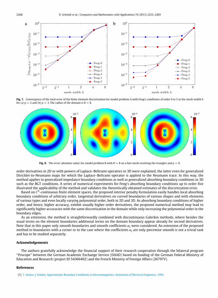
The results of the convergence analysis are shown in Fig. 6. The observed convergence orders of the discretization errorin the H1(Ω)-seminorm are 1.0 for p = 1, 2.0 for p = 2 and 3.0 for p = 3, and in the L2(Ω)-norm 2.0 for p = 1, 3.0 forp = 2 and 4.0 for p = 3. Hence, the convergence orders meet the orders of the best-approximation error. In the variationalformulation with Feng’s conditions integrals of the trace of the solution and its derivatives on the outer boundary Γ arepresent. Therefore, the convergence of the discretization error on Γ is studied as well. In the H1(Γ )-seminorm the obtainedconvergence rates are 1.2, 2.0 and 3.0 for p = 1, 2, 3, respectively, and correlate to the convergence orders of the best-approximation error. In the L2(Γ )-norm convergence rates of 2.0, 4.0, and 5.3 for p = 1, 2, 3, respectively, are observed.These observed convergence rates are for p = 2 and p = 3 better than those for the best-approximation error of an arbitrary,smooth enough function (see Fig. 5).Modelling error for model problem B. For model problem B Feng’s conditions of different order for a fine mesh withpolynomial p = 6 are compared. Here, the discretization error is less than 1 · 10−6 in L∞(Ω) and the modelling error isdominating. In Fig. 8 the modelling error for R = 8 using the Feng-0 condition, which is of Robin type, the Feng-2 condition,which is of Wentzell type, and the Feng-4 condition are shown. Increasing the order of the condition leads to a significanterror reduction, the error diminishes by a factor of 100 when using Feng-2 instead of Feng-0, and by another factor of 10when using Feng-4 instead of Feng-2. For the parameters used the Feng-5 conditions do not give a further error reduction.This will only be achieved for larger domain radius R.Total error for model problem A. Using the proposed finite element method for the scattering using Feng’s conditions thediscrete solution compromises a discretization error and a modelling error, which in sum can be called the total error. Totalerror is studied for the model problem A with a fixed domain Ω with R = 8, and uniform polynomial degrees p = 2, 3. The


a b

Fig. 5. Convergence of the relative discretization error in (a) the H1(Ω)-seminorm, and (b) the L2(Ω)-norm for the nonconforming Galerkin formulationwith polynomial order p = 1 to p = 3 for the Feng-5 conditions for the model problem A, where RD = 1 and R = 8.

a b

Fig. 6. Convergence of the relative discretization error in (a) the H1(Ω)-seminorm, and (b) the L2(Ω)-norm for the nonconforming Galerkin formulationwith polynomial order p = 1 to p = 3 for the Feng-5 conditions for the model problem A, where RD = 1 and R = 3.

total L2(Ω)-error as a function of the mesh-width h for Feng’s conditions up to order 5 are shown in Fig. 7. Before reachingthe level of themodelling error, the total error decays likeO(h3) orO(h4) for p = 2 or p = 3, respectively. In this study,wherethe domain is fixedwith R large enough, the error reduceswithmesh refinement due to a decrease of the discretization errorand saturates on the level of the modelling error. To obtain a certain level of the total error level the refinement of meshmight not be sufficient, where then either a higher order Feng condition has to be used or the radius of the domain has tobe increased.

7. Conclusion

A new finite element method for high-order absorbing boundary conditions was proposed. It combines the classicalC0-continuous finite element discretization with bilinear forms adopted from discontinuous Galerkin methods for thediscretization of the high-order differential operators on the boundary. As there is no need to introduce any auxiliary variableor basis functionswith higher regularity, themethod is simply integrated into establishedhigh-order finite element libraries.In this article, the case of symmetric absorbing boundary conditions in 2D, for which only derivatives of even orders arepresent, was completely analysed, where we showed that the discretization of the higher-order operators does not hamperthe convergence of the finite element method as long as the polynomial degree on the boundary is increased with the orderof the boundary condition.More precisely, for each second derivative higher than two the polynomial order on the boundaryhas to be increased by one, and the same convergence rate as for lower order boundary conditions like the Dirichlet,Neumann, Robin or even Wentzell conditions is obtained. In addition, the changes in the method with additional odd


a b

Fig. 7. Convergence of the total error of the finite element discretization for model problem A with Feng’s conditions of order 0 to 5 in the mesh-width hfor (a) p = 2 and (b) p = 3. The radius of the domain is R = 8.

0

2

4

6

0

2

4

6

0

2

4

6⋅10–5⋅10–2 ⋅10–4

Fig. 8. The error (absolute value) for model problem B with R = 8 on a fine mesh resolving the triangles and p = 6.

order derivatives in 2D or with powers of Laplace–Beltrami operators in 3D were explained, the latter even for generalizedDirichlet-to-Neumann maps for which the Laplace–Beltrami operator is applied to the Neumann trace. In this way, themethod applies to generalized impedance boundary conditions as well as generalized absorbing boundary conditions in 3Dsuch as the BGT conditions. A series of numerical experiments for Feng’s absorbing boundary conditions up to order fiveillustrated the applicability of the method and validates the theoretically obtained estimates of the discretization error.

Based on C0-continuous finite element spaces, the proposed interior penalty formulation easily handles local absorbingboundary conditions of arbitrary order, tangential derivatives on curved boundaries of various shapes and with elementsof various types and even locally varying polynomial order, both in 2D and 3D. As absorbing boundary conditions of higherorder, and hence, higher accuracy, exhibit usually higher order derivatives, the proposed numerical method may lead tosignificantly higher accuracies with the same discretization in the domain while only increasing the polynomial order in theboundary edges.

As an extension, the method is straightforwardly combined with discontinuous Galerkin methods, where besides theusual terms on the element boundaries additional terms on the domain boundary appear already for second derivatives.Note that in this paper only smooth boundaries and smooth coefficients αj were considered. An extension of the proposedmethod to boundaries with a corner or to the case where the coefficients αj are only piecewise smooth is not a trivial taskand has to be studied separately.

Acknowledgements

The authors gratefully acknowledge the financial support of their research cooperation through the bilateral program‘‘Procope’’ between the German Academic Exchange Service (DAAD) based on funding of the German Federal Ministry ofEducation and Research (project ID 54366492) and the French Ministry of Foreign Affairs (26797V).

References

[1] T. Senior, J. Volakis, Approximate Boundary Conditions in Electromagnetics, Institution of Electrical Engineers, 1995.

http://refhub.elsevier.com/S0898-1221(15)00413-7/sbref1


[2] F. Ihlenburg, Finite Element Analysis of Acoustic Scattering, Springer-Verlag, 1998.[3] S. Yuferev, N. Ida, Surface Impedance Boundary Conditions: A Comprehensive Approach, CRC Press, 2010.[4] D. Givoli, I. Patlashenko, J.B. Keller, High-order boundary conditions and finite elements for infinite domains, Comput. Methods Appl. Mech. Engrg.

143 (1–2) (1997) 13–39.[5] K. Schmidt, C. Heier, An analysis of Feng’s and other symmetric local absorbing boundary conditions, ESAIMMath. Model. Numer. Anal. 49 (1) (2015)

257–273.[6] V. Bonnaillie-Noël, M. Dambrine, F. Hérau, G. Vial, On generalized Ventcel’s type boundary conditions for Laplace operator in a bounded domain,

SIAM J. Math. Anal. 42 (2) (2010) 931–945.[7] M. Wang, C. Engström, K. Schmidt, C. Hafner, On high-order FEM applied to canonical scattering problems in plasmonics, J. Comput. Theor. Nanosci.

8 (2011) 1–9.[8] D. Givoli, J.B. Keller, Special finite elements for use with high-order boundary conditions, Comput. Methods Appl. Mech. Engrg. 119 (3–4) (1994)

199–213.[9] D. Givoli, High-order nonreflecting boundary conditions without high-order derivatives, J. Comput. Phys. 170 (2) (2001) 849–870.

[10] D. Givoli, High-order local non-reflecting boundary conditions: a review, Wave Motion 39 (4) (2004) 319–326.[11] M. Grote, A. Schneebeli, D. Schötzau, Discontinuous Galerkin finite element method for the wave equation, SIAM J. Numer. Anal. 44 (6) (2006)

2408–2431.[12] S. Brenner, L.-Y. Sung, C0 interior penalty methods for fourth order elliptic boundary value problems on polygonal domains, J. Sci. Comput. 22–23

(1–3) (2005) 83–118.[13] D. Givoli, Non-reflecting boundary conditions, J. Comput. Phys. 94 (1) (1991) 1–29.[14] T. Senior, Impedance boundary conditions for imperfectly conducting surfaces, Appl. Sci. Res. (B) 8 (1) (1960) 418–436.[15] S. Rytov, Calculation of skin effect by perturbation method, Zh. Exp. Teor. Fiz. 10 (1940) 180–189.[16] M.A. Leontovich, On approximate boundary conditions for electromagnetic fields on the surface of highly conducting bodies, in: Research in the

Propagation of Radio Waves, Academy of Sciences of the USSR, Moscow, 1948, pp. 5–12. (in Russian).[17] H. Haddar, P. Joly, H. Nguyen, Generalized impedance boundary conditions for scattering by strongly absorbing obstacles: the scalar case,Math.Models

Methods Appl. Sci. 15 (8) (2005) 1273–1300.[18] S. Yuferev, L. Di Rienzo, Surface impedance boundary conditions in terms of various formalisms, IEEE Trans. Magn. 46 (9) (2010) 3617–3628.[19] B. Engquist, J.-C. Nédélec, Effective boundary conditions for acoustic and electromagnetic scattering in thin layers. Tech. Rep, Ecole Polytechnique

Paris, 1993, Rapport interne du C.M.A.P.[20] A. Bendali, K. Lemrabet, The effect of a thin coating on the scattering of a time-harmonic wave for the Helmholtz equation, SIAM J. Appl. Math. 6 (1996)

1664–1693.[21] C. Poignard, Asymptotics for steady-state voltage potentials in a bidimensional highly contrasted medium with thin layer, Math. Methods Appl. Sci.

31 (4) (2008) 443–479.[22] B. Aslanyürek, H. Haddar, H. Şahintürk, Generalized impedance boundary conditions for thin dielectric coatings with variable thickness, WaveMotion

48 (7) (2011) 681–700.[23] K. Schmidt, A. Thöns-Zueva, Impedance boundary conditions for acoustic time harmonic wave propagation in viscous gases, (2014), Manuscript

submitted for publication.[24] K. Schmidt, A. Chernov, A unified analysis of transmission conditions for thin conducting sheets in the time-harmonic eddy current model, SIAM J.

Appl. Math. 73 (6) (2013) 1980–2003.[25] B. Delourme, H. Haddar, P. Joly, Approximatemodels for wave propagation across thin periodic interfaces, J. Math. Pures Appl. (9) 98 (1) (2012) 28–71.[26] T.B.A. Senior, Generalized boundary and transition conditions and the question of uniqueness, Radio Sci. 27 (6) (1992) 929–934.[27] M.F. Wheeler, An elliptic collocation-finite element method with interior penalties, SIAM J. Numer. Anal. 15 (1) (1978) 152–161.[28] B. Rivière, M.F. Wheeler, V. Girault, A priori error estimates for finite element methods based on discontinuous approximation spaces for elliptic

problems, SIAM J. Numer. Anal. 39 (3) (2001) 902–931.[29] S. Sun, M.F. Wheeler, Symmetric and nonsymmetric discontinuous Galerkin methods for reactive transport in porous media, SIAM J. Numer. Anal. 43

(1) (2005) 195–219.[30] V.A. Kozlov, V.G. Maz’ya, J. Rossmann, Elliptic Boundary Value Problems in Domains with Point Singularities, in: Mathematical Surveys and

Monographs, vol. 52, American Mathematical Society, Providence, RI, 1997.[31] C. Schwab, p- and hp-Finite Element Methods: Theory and Applications in Solid and Fluid Mechanics, Oxford University Press, Oxford, UK, 1998.[32] T. Hagstrom, T. Warburton, A new auxiliary variable formulation of high-order local radiation boundary conditions: corner compatibility conditions

and extensions to first-order systems, Wave Motion 39 (4) (2004) 327–338.[33] T. Hagstrom, A. Mar-Or, D. Givoli, High-order local absorbing conditions for the wave equation: Extensions and improvements, J. Comput. Phys. 227

(6) (2008) 3322–3357.[34] J.-C. Nédélec, Acoustic and Electromagnetic Equations, in: Applied Mathematical Sciences, vol. 144, Springer Verlag, 2001.[35] A. Bayliss, M. Gunzburger, E. Turkel, Boundary conditions for the numerical solution of elliptic equations in exterior regions, SIAM J. Appl. Math. 42

(2) (1982) 430–451.[36] X. Antoine, H. Barucq, A. Bendali, Bayliss–Turkel-like radiation conditions on surfaces of arbitrary shape, J. Math. Anal. Appl. 229 (1) (1999) 184–211.[37] H. Barucq, R. Djellouli, A. Saint-Guirons, Three-dimensional approximate local DtN boundary conditions for prolate spheroid boundaries, J. Comput.

Appl. Math. 234 (6) (2010) 1810–1816.[38] I. Patlashenko, D. Givoli, Non-reflecting finite element schemes for three-dimensional acoustic waves, J. Comput. Acoust. 5 (1) (1997) 95–115.[39] I. Harari, Computational methods for problems of acoustics with particular reference to exterior domains (Ph.D. thesis), Stanford University, Stanford,

USA, 1988.[40] T. Warburton, J.S. Hesthaven, On the constants in hp-finite element trace inverse inequalities, Comput. Methods Appl. Mech. Engrg. 192 (2003)

2765–2773.[41] R.A. Adams, Sobolev Spaces, Academic Press, New-York, London, 1975.[42] S. Sauter, C. Schwab, Boundary Element Methods, Springer-Verlag, Heidelberg, 2011.[43] J.M. Melenk, S. Sauter, Wavenumber explicit convergence analysis for Galerkin discretizations of the Helmholtz equation, SIAM J. Numer. Anal. 49 (3)

(2011) 1210–1243.[44] I. Babuška, J. Osborn, Eigenvalue problems, in: Handbook of Numerical Analysis, Vol. II, North-Holland, 1991, pp. 641–787. (Chapter).[45] A.H. Schatz, An observation concerning Ritz–Galerkin methods indefinite bilinear forms, Math. Comp. 28 (1974) 959–962.[46] S. Brenner, L. Scott, The Mathematical Theory of Finite Element Methods, Springer-Verlag, New York, 1994.[47] P. Ciarlet, The Finite Element Method for Elliptic Problems, in: Studies in Mathematics and its Applications, vol. 4, North-Holland, Amsterdam, 1978.[48] P. Frauenfelder, C. Lage, Concepts—an object-oriented software package for partial differential equations, M2AN Math. Model. Numer. Anal. 36 (5)

(2002) 937–951.[49] Concepts Development Team. Webpage of Numerical C++ Library Concepts 2, 2015. http://www.concepts.math.ethz.ch.[50] K. Schmidt, P. Kauf, Computation of the band structure of two-dimensional photonic crystals with hp finite elements, Comput. Methods Appl. Mech.

Engrg. 198 (2009) 1249–1259.[51] A.L. Koh, A.I. Fernández-Domínguez, D.W. McComb, S.A. Maier, J.K. Yang, High-resolution mapping of electron-beam-excited plasmon modes in

lithographically defined gold nanostructures, Nano Lett. 11 (3) (2011) 1323–1330.















































http://www.concepts.math.ethz.ch



hal.inria.fr · hal id: hal-01184251 submitted on 13 jan 2016 hal is a multi-disciplinary open...

Documents