HAL Id: inria-00193865https://hal.inria.fr/inria-00193865v3

Submitted on 27 Jan 2009

HAL is a multi-disciplinary open accessarchive for the deposit and dissemination of sci-entific research documents, whether they are pub-lished or not. The documents may come fromteaching and research institutions in France orabroad, or from public or private research centers.

L’archive ouverte pluridisciplinaire HAL, estdestinée au dépôt et à la diffusion de documentsscientifiques de niveau recherche, publiés ou non,émanant des établissements d’enseignement et derecherche français ou étrangers, des laboratoirespublics ou privés.

An H∞ LPV Design for Sampling Varying Controllers :Experimentation with a T Inverted Pendulum

David Robert, Olivier Sename, Daniel Simon

To cite this version:David Robert, Olivier Sename, Daniel Simon. An H∞ LPV Design for Sampling Varying Controllers :Experimentation with a T Inverted Pendulum. [Research Report] RR-6380, INRIA. 2007, pp.25.�inria-00193865v3�

appor t de r ech er ch e

ISS

N02

49-6

399

ISR

NIN

RIA

/RR

--63

80--

FR

+E

NG

Thème NUM

INSTITUT NATIONAL DE RECHERCHE EN INFORMATIQUE ET EN AUTOMATIQUE

An H∞ LPV Design for Sampling VaryingControllers : Experimentation with a T Inverted

Pendulum

David Robert — Olivier Sename — Daniel Simon

N° 6380

Décembre 2007

Centre de recherche Inria de Grenoble – Rhône-Alpes655, avenue de l’Europe, 38334 Montbonnot Saint Ismier (France)

Téléphone : +33 4 76 61 52 00 — Télécopie +33 4 76 61 52 52

An H∞ LPV Design for Sampling VaryingControllers : Experimentation with a T InvertedPendulumDavid Robert ∗†, Olivier Sename∗† , Daniel Simon ‡†Thème NUM � Systèmes numériquesÉquipe-Projet NeCSRapport de re her he n° 6380 � Dé embre 2007 � 25 pagesAbstra t: "This work has been submitted to the IEEE for possible publi- ation. Copyright may be transferred without noti e, after whi h this versionmay no longer be a essible."This report deals with the adaptation of a real-time ontroller's samplingperiod to a ount for the available omputing resour e variations. The designof su h ontrollers requires a parameter-dependent dis rete-time model of theplant, where the parameter is the sampling period. A polytopi approa h forLPV (Linear Parameter Varying) systems is then developed to get an H∞ sam-pling period dependent ontroller. A redu tion of the polytope size is here per-formed whi h drasti ally redu es the onservatism of the approa h and makeseasier the ontroller implementation. Some experimental results on a T invertedpendulum are provided to show the e� ien y of the approa h.Key-words: Digital ontrol, linear parameter varying systems, H∞ ontrol,real experiments.

∗ GIPSA-lab (Control Systems Dpt.), UMR INPG-CNRS 5216, ENSIEG-BP 46, 38402Saint Martin d'Hères Cedex, Fran e† This work is partially supported by the Safe_NeCS proje t funded by the ANR undergrant ANR-05-SSIA-0015-03‡ INRIA Rh�ne-Alpes, Inovallée 655 avenue de l'Europe, Montbonnot, 38334 Saint-IsmierCedex, Fran e

Une méthode de on eption de ontr�leurs àpériode d'é hantillonage variable LPV H∞ :appli ation à un pendule inverséRésumé : Ce rapport examine le problème de l'adaptation en temps-réel dela période d'é hantillonnage d'un ontr�leur, a�n de lui permettre de s'adapteraux variations de la ressour e de al ul disponible. La on eption du ontr�-leur né essite d'avoir un modèle en temps dis ret paramétré du pro édé, où leparamètre variable est la période d'é hantillonnage. Une méthode basée surl'appro he polytopique (LPV) est utilisée pour synthétiser un ontr�leur H∞ àpériode variable. L'utilisation d'un polytope de taille réduite permet de réduirefortement le onservatisme et la omplexité de re onstru tion du ontr�leur. Laméthode est validée expérimentalement sur un pendule inversé.Mots- lés : Commande numérique, systèmes à paramètres variables, om-mande H∞, validation expérimentale

An H∞ LPV Design for Sampling Varying Controllers : Experimentation with a T Inverted Pendulum31 Introdu tionHigh-te hnology appli ations ( ars, household applian es..) are using more andmore omputing and network resour es, leading to a need of onsumption op-timisation for de reasing the ost or enhan ing reliability and performan es. Asolution is to improve the �exibility of the system by on-line adaptation of thepro essor/network utilisation, either by hanging the algorithm or by adaptingthe sampling period. This paper deals with the latter ase and presents thesynthesis of a ontrol law with varying sampling period.Few re ent works have been devoted to the omputing resour e variations.In [1℄ a feedba k ontroller with a sampling period dependent PID ontroller isused. In [2, 3℄ a feedba k s heduler based on a LQ optimisation of the ontroltasks periods is proposed. In [4℄ a pro essor load regulation is proposed andapplied for real-time ontrol of a robot arm. The design of a sampling perioddependent RST ontroller was proposed in [5℄. This latter paper dealt with the ontrol of linear SISO systems at a variable sampling rate, and its promisingresults alled for extensions towards multivariable systems.The presented ontribution enhan es a previous paper ([6℄) using a linearparameter-varying (LPV) approa h of the linear robust ontrol framework [7℄.The LPV approa h primarily deals with variations of the plant's parameters,although it has been applied also to a plant parameter dependent sampling viaa lifting te hnique as in [8℄.This paper provides a methodology for designing a sampling period depen-dent ontroller with performan e adaptation, whi h an be used in the ontextof embedded ontrol systems. First we propose a parametrised dis retization ofthe ontinuous time plant and of the weighting fun tions, leading to a dis rete-time sampling period dependent augmented plant. In parti ular the plant dis- retization approximates the matrix exponential by a Taylor series of order N .Therefore we obtain a polytopi LPV model made of 2N verti es, as presentedin [6℄. In this paper we exploit the dependen y between the variables param-eters, whi h are the su essive powers of the sampling period h, h2, ..., hN , toredu e the number of ontrollers to be ombined to N + 1. The H∞ ontroldesign method for polytopi models [7℄ is then used to get a sampling perioddependent dis rete-time ontroller. The redu tion of the polytopi set drasti- ally de reases both the omplexity and the onservatism of the previous workand makes the solution easier to implement. This approa h is then validated byexperiments on real-time ontrol of a T inverted pendulum.The outline of this paper is as follows. Se tion 2 des ribes the plant dis- retization and the redu tion of the original omplexity using the parametersdependen y. In se tion 3 the losed-loop obje tives are stated and expressedas weighting fun tions in the H∞ framework. Se tion 4 omments brie�y theaugmented plant and gives ba kground on H∞/LPV ontrol design. The exper-iments on the "T" inverted pendulum are des ribed in se tion 5. Finally, thepaper ends with some on lusions and further resear h dire tions.2 A sample dependent LPV dis rete-time modelIn this se tion the way to obtain a polytopi dis rete-time model, the parameterof whi h being the sampling period, is detailed.RR n° 6380

4 Robert, Sename & SimonWe onsider a state spa e representation of ontinuous time plants as :G :

{

x = Ax + Buy = Cx + Du

(1)where x ∈ Rn, u ∈ R

m and y ∈ Rp. The exa t dis retization of this systemwith a zero order hold at the sampling period h leads to the dis rete-time LPVsystem (2)

Gd :

{

xk+1 = Ad(h) xk + Bd(h) uk

yk = Cd(h) xk + Dd(h) uk(2)with

Ad = eAh Bd =

∫ h

0

eAτdτB

Cd = C Dd = D

(3)The state spa e matri es are usually omputed using expression (4) and (5),see [9℄.(

Ad Bd

0 I

)

= exp

((

A B0 0

)

h

) (4)Cd = C Dd = D (5)with h ranging in [hmin; hmax]1. However in (4) Ad and Bd are not a�ne on h.2.1 Preliminary approa h: Taylor expansionOur aim is to get a polytopi model in order to satisfy one of the frameworksof H∞ ontrol for LPV systems. We here propose to approximate the matrixexponential by a Taylor series of order N as :Ad(h) ≈ I +

N∑

i=1

Ai

i!hi (6)

Bd(h) ≈

N∑

i=1

Ai−1B

i!hi (7)However it is well known that the Taylor approximation is valid only for param-eters near zero. As h is assumed to belong to the interval [hmin, hmax℄ with

hmin > 0 the approximation will be onsidered around the nominal value h0 ofthe sampling period, as:h = h0 + δ with hmin − h0 ≤ δ ≤ hmax − h0 (8)Then we get:

(

Ad Bd

0 I

)

=

(

Ah0Bh0

0 I

) (

Aδ Bδ

0 I

) (9)1the variable sampling period should be hosen in a range where the ontrol performan eis highly sensitive w.r.t. to the sampling rate, e.g. a ording to the rule of thumb ωcl h ≈

0.2 . . . 0.6 where ωcl is the desired losed-loop frequen y [9℄ INRIA

An H∞ LPV Design for Sampling Varying Controllers : Experimentation with a T Inverted Pendulum5where(

Ah0Bh0

0 I

)

= exp

((

A B0 0

)

h0

)

,

(

Aδ Bδ

0 I

)

= exp

((

A B0 0

)

δ

)This leads toAd = Ah0

Aδ

Bd = Bh0+ Ah0

Bδ

(10)Remark 1 When δ = 0, then Aδ = I and Bδ = 0 whi h means that, asexpe ted, Ad = Ah0and Bd = Bh0

.As h0 is known at design time and onstant, the Taylor approximation isthen used only for Aδ and Bδ, as:Ad(h) ≈ Ah0

(I +

N∑

i=1

Ai

i!δi) := Ad(δ) (11)

Bd(h) ≈ Bh0+ Ah0

(

N∑

i=1

Ai−1B

i!δi) := Bd(δ) (12)To evaluate the approximation error due to the Taylor approximation, a riterion based on the H∞ norm is hosen here to express the worst ase errorbetween Gde

and Gd, both dis rete-time models using respe tively the exa tmethod and the approximated one (i.e. the Taylor series approximation oforder N).JN = max

hmin<h<hmax

‖ Gde(h, z) − Gd(h, z) ‖∞ (13)2.2 A �rst polytopi modelAs h belongs to the interval [hmin, hmax℄, then we an de�ne H = [δ, δ2, . . . , δN ]the ve tor of parameters. H belongs to a onvex polytope (hyper-polygon) H(14) with 2N verti es,.

H =

2N

∑

i=1

αi(δ)ωi : αi(δ) ≥ 0,2

N

∑

i=1

αi(δ) = 1

(14){δ, δ2, . . . , δN}, δi ∈ {δi

min, δimax} (15)Ea h vertex is de�ned by a ve tor ωi = [νi1 , νi2 , . . . , νiN

] where νij an takethe extremum values {δj

min, δjmax} with δmin = hmin−h0 and δmax = hmax−h0.The matri es Ad(δ) and Bd(δ) are therefore a�ne in H and given by thepolytopi forms:

Ad(H) =2

N

∑

i=1

αi(δ)Adi, Bd(H) =

2N

∑

i=1

αi(δ)Bdiwhere the matri es at the verti es, i.e. Adiand Bdi

, are obtained by the al ulation of Ad(δ) and Bd(δ) at ea h vertex of the polytope H. The polytopi RR n° 6380

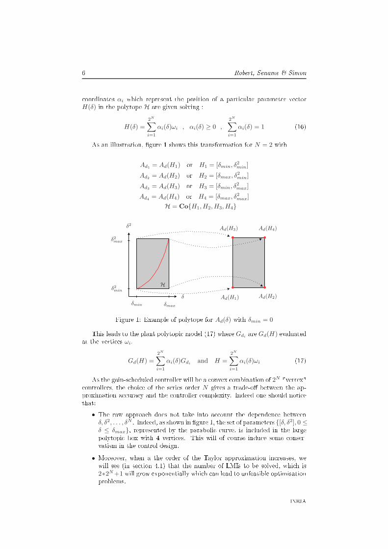
6 Robert, Sename & Simon oordinates αi whi h represent the position of a parti ular parameter ve torH(δ) in the polytope H are given solving :

H(δ) =

2N

∑

i=1

αi(δ)ωi , αi(δ) ≥ 0 ,

2N

∑

i=1

αi(δ) = 1 (16)As an illustration, �gure 1 shows this transformation for N = 2 withAd1

= Ad(H1) or H1 = [δmin, δ2min]

Ad2= Ad(H2) or H2 = [δmax, δ2

min]

Ad3= Ad(H3) or H3 = [δmin, δ2

max]

Ad4= Ad(H4) or H4 = [δmax, δ2

max]

H = Co{H1, H2, H3, H4}

δmin δmax

δ

δ2

δ2min

δ2max

H

b b

bb

b

Ad(H1) Ad(H2)

Ad(H4)Ad(H3)

Figure 1: Example of polytope for Ad(δ) with δmin = 0This leads to the plant polytopi model (17) where Gdiare Gd(H) evaluatedat the verti es ωi.

Gd(H) =2

N

∑

i=1

αi(δ)Gdiand H =

2N

∑

i=1

αi(δ)ωi (17)As the gain-s heduled ontroller will be a onvex ombination of 2N "vertex" ontrollers, the hoi e of the series order N gives a trade-o� between the ap-proximation a ura y and the ontroller omplexity. Indeed one should noti ethat:� The raw approa h does not take into a ount the dependen e betweenδ, δ2, . . . , δN . Indeed, as shown in �gure 1, the set of parameters {[δ, δ2], 0 ≤δ ≤ δmax}, represented by the paraboli urve, is in luded in the largepolytopi box with 4 verti es. This will of ourse indu e some onser-vatism in the ontrol design.� Moreover, when a the order of the Taylor approximation in reases, wewill see (in se tion 4.1) that the number of LMIs to be solved, whi h is2∗2N +1 will grow exponentially whi h an lead to unfeasible optimisationproblems. INRIA

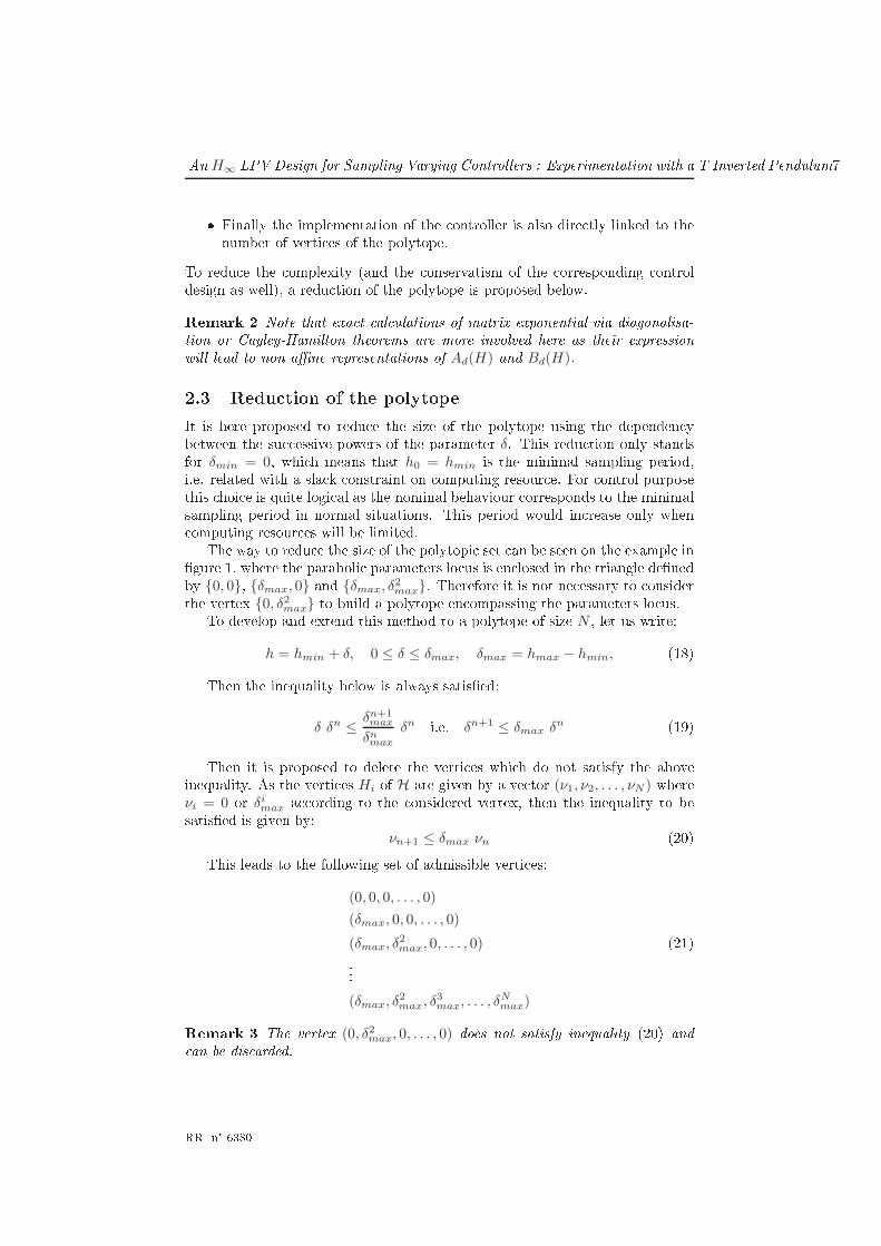
An H∞ LPV Design for Sampling Varying Controllers : Experimentation with a T Inverted Pendulum7� Finally the implementation of the ontroller is also dire tly linked to thenumber of verti es of the polytope.To redu e the omplexity (and the onservatism of the orresponding ontroldesign as well), a redu tion of the polytope is proposed below.Remark 2 Note that exa t al ulations of matrix exponential via diagonalisa-tion or Cayley-Hamilton theorems are more involved here as their expressionwill lead to non a�ne representations of Ad(H) and Bd(H).2.3 Redu tion of the polytopeIt is here proposed to redu e the size of the polytope using the dependen ybetween the su essive powers of the parameter δ. This redu tion only standsfor δmin = 0, whi h means that h0 = hmin is the minimal sampling period,i.e. related with a sla k onstraint on omputing resour e. For ontrol purposethis hoi e is quite logi al as the nominal behaviour orresponds to the minimalsampling period in normal situations. This period would in rease only when omputing resour es will be limited.The way to redu e the size of the polytopi set an be seen on the example in�gure 1, where the paraboli parameters lo us is en losed in the triangle de�nedby {0, 0}, {δmax, 0} and {δmax, δ2max}. Therefore it is not ne essary to onsiderthe vertex {0, δ2

max} to build a polytope en ompassing the parameters lo us.To develop and extend this method to a polytope of size N , let us write:h = hmin + δ, 0 ≤ δ ≤ δmax, δmax = hmax − hmin, (18)Then the inequality below is always satis�ed:

δ δn ≤δn+1max

δnmax

δn i.e. δn+1 ≤ δmax δn (19)Then it is proposed to delete the verti es whi h do not satisfy the aboveinequality. As the verti es Hi of H are given by a ve tor (ν1, ν2, . . . , νN) whereνi = 0 or δi

max a ording to the onsidered vertex, then the inequality to besatis�ed is given by:νn+1 ≤ δmax νn (20)This leads to the following set of admissible verti es:

(0, 0, 0, . . . , 0)

(δmax, 0, 0, . . . , 0)

(δmax, δ2max, 0, . . . , 0) (21)...

(δmax, δ2max, δ3

max, . . . , δNmax)Remark 3 The vertex (0, δ2

max, 0, . . . , 0) does not satisfy inequality (20) and an be dis arded.RR n° 6380

8 Robert, Sename & SimonThis method leads to a set of N + 1 verti es instead of 2N . Note that theseverti es are linearly independent and make a simplex, whi h is itself basi ally apolytope [10℄ of minimal dimension onsidering the parameters spa e of dimen-sion N.When N = 2 (and for 0 < δ < δmax) the square is downsized to the trianglein �gure 2. When N = 3 the pyramid in �gure 3 is the redu tion of a ube.

Figure 2: Polytope redu tion for N=2

Figure 3: Polytope redu tion for N=33 Formulation of the H∞/LPV ontrol problemIn this se tion we �rst present the formulation of the H∞ ontrol problem usingweighting fun tion depending on the sampling period. Indeed the providedmethodology will allow for performan e adaptation a ording to the omputingresour es availability.The H∞ framework is based on the general ontrol on�guration of �gure 4,where Wi and Wo are some weighting fun tions representing the spe i� ationof the desired losed-loop performan es (see [11℄). The obje tive is here to �nda ontroller K su h internal stability is a hieved and ‖z‖2 < γ‖w‖2, where γrepresents the H∞ attenuation level. INRIA

An H∞ LPV Design for Sampling Varying Controllers : Experimentation with a T Inverted Pendulum9- ---

�

-

WoWi

K

z

y

w

u

zw

P

P

Figure 4: Fo used inter onne tion3.1 Towards dis rete-time weighting fun tionsClassi al ontrol design assumes onstant performan e obje tives and produ esa ontroller with an unique sampling period. The sampling period is hosena ording to the ontroller bandwidth, the noise sensibility and the availabilityof omputation resour es. When the sampling period varies the usable ontrollerbandwidth also varies and the losed-loop obje tives should logi ally be adapted.Therefore we propose to adapt the bandwidth of the weighting fun tions to thesampling period.The methodology is as follows. First Wi and Wo are split into two parts :� a onstant part with onstant poles and zeros. This allows, for instan e,to ompensate for os illations or �exible modes whi h are, by de�nition,independent of the sampling period.� the variable part ontains poles and zeros whose pulsations are expressedas an a�ne fun tion of the sampling frequen y f = 1/h. This allows for anadaption of the bandwidth of the weighting fun tions, and hen e for anadaption of the losed-loop performan e w.r.t. the available omputingpower. These poles and zeros are here onstrained to be real by thedis retization step.First of all the onstant parts of the weighting fun tions are merged withthe ontinuous-time plant model. Then a dis rete-time augmented system isdeveloped as presented above.The variable part V (s) of a weighting fun tion is the dis retized a ordingto the following methodology:1. fa torise V (s) as a produ t of �rst order systems. We here hose polesand zeros depending linearly of the sampling frequen y f = 1/h, as:V (s) = β

∏

i

s − bif

s − aif= β

∏

i

Vi(s) (22)with ai, bi ∈ R2. Consider the state spa e observable anoni al form for Vi(s)

Vi(s) :

{

xi = aif xi + f(ai − bi) ui

yi = xi + ui

(23)RR n° 6380

10 Robert, Sename & Simon3. form the series inter onne tion of the state spa e representation of ea hVi(s). This allows to get V (s) of the form (24) with appropriate dimensionsof the state spa e matri es.

V (s) :

{

xv = Avf xv + Bvf uv

yv = Cv xv + Dv uv(24)4. Get the dis rete-time state spa e representation of V (s). Thanks to thea�ne dependen e in f in (24) the dis rete-time model of the variable partbe omes independent of h sin e:

Avd= eAvf h = eAv

Bvd= (Avf)−1(Avd

− I)Bvf = (Av)−1(Avd− I)Bv

Cvd= Cv and Dvd

= Dv

(25)Remark 4 The serial inter onne tion of two systems of the form (26) leads toa system of the form (27).{

x = Af x + Bf u

y = C x + D u(26)

A =

(

A1 0B2C1 A2

)

B =

(

B1

B2D1

)

x =

(

x1

x2

)

C =(

D2C1 C2

)

D = D2D1

(27)As seen matri es C and D only depend on Ci or Di, i = 1, 2, whi h ensuresthat they do not depend on f . Then there is no oupling between Ai and Bi,i = 1, 2, whi h keeps the linear dependen e on f of the state spa e equation. Asillustration and forward, the inter onne tion of 3 systems leads to a state spa erepresentation (28) :

A =

A1 0 0B2C1 A2 0

B3D2C1 B3C2 A3

B =

B1

B2D1

B3D2D1

x =

x1

x2

x3

C =(

D3D2C1 D3C2 C3

)

D = D3D2D1

(28)By iteration, the serial inter onne tion of more than three systems (26) stillkeeps the form (26). Therefore the inter onne tion of systems Vi(p) whi h arein form (26) leads to a system in the form (24) where the dependen e on fmakes easier the dis retization step.Remark 5 The simpli� ation between f and h in (25) makes easy the dis- retization step. This is why the plant and the weighting fun tions are separatelydis retized, and the augmented plant is obtained in dis rete time afterwards byinter onne tion. This is also a onsequen e of the use of the observable anoni alform.INRIA

An H∞ LPV Design for Sampling Varying Controllers : Experimentation with a T Inverted Pendulum113.2 The dis rete-time augmented plantLet us here present the overall methodology to get the dis rete-time plant in-ter onne tion.Let �rst onsider the following ontinuous-time model where the onstantpart of the weighting fun tion Wi and Wo has been onne ted to the plantmodel:P :

x(t) = Ax(t) + Bww(t) + Buu(t)

z(t) = Czx(t) + Dzww(t) + Dzuu(t)

y(t) = Cyx(t) + Dyww(t) + Dyuu(t)

(29)where x ∈ Rn is the state, w ∈ Rmw represents the exogenous inputs, u ∈ Rmuthe ontrol inputs, z ∈ Rpz the ontrolled output and y ∈ Rpy the measurementve tor.A dis rete-time representation of the above system is �rst obtained thanksto the previous methodology. For simpli ity we will note, a ording to therepresentation (1):A = A B =

(

Bw Bu

)

C =

(

Cz

Cy

)

D =

(

Dzw Dzu

Dyw Dyu

) (30)Using the Taylor approximation at order N leads to a polytope H. Thispolytope has r verti es (where r equals 2N for the basi ase and N + 1 for theredu ed one). Ea h of the r verti es is des ribed by a ve tor ωi of the form(δ1, δ2, . . . , δr) where δi = δi

min or δimax.The LPV polytopi dis rete-time model is given by:

P(H) :

xk+1 = A(H)xk + Bw(H)w + Bu(H)u

z = Czxk + Dzww + Dzuu

y = Cyxk + Dyww + Dyuu

(31)H =

(

δ δ2 . . . δN)

H ∈ H = Co{ω1, . . . , ωr}

H =

r∑

i=1

αiωi A(H) =

r∑

i=1

αiAi

r∑

i=1

αi = 1 αi ≥ 0(32)where, a ording to the representation (2)

Ad = A Bd =(

Bw Bu

)

Cd = C Dd = D (33)Now, the variable part of the weighting fun tions Wi and Wo are expressedas previously presented, whi h leads to both dis rete-time representations (34)and(35) where the size of the state ve tor depend on the weighting fun tion:WI :

{

xIk+1= AIxIk

+ BIw

w = CIxIk+ DIw

(34)WO :

{

xOk+1= AOxOk

+ BOz

z = COxOk+ DOz

(35)RR n° 6380

12 Robert, Sename & SimonThe augmented system P ′(H) is obtained by the inter onne tion of P(H),WI and WO. Therefore we obtain the following LPV polytopi dis rete-timesystem of state ve tor x′

k = (xk xIkxOk

)T :P ′(H) :

x′

k+1 = A′(H)x′

k + B′

w(H)w + B′

u(H)u

z = C′

zx′

k + D′

zww + D′

zuu

y = C′

yx′

k + D′

yww + D′

yuu

(36)withA′(H) =

A(H) Bw(H)CI 00 AI 0

BOCz BODzwCI AO

B′

w(H) =

Bw(H)DI

BI

BODzwDI

B′

u(H) =

Bu(H)0

BODzu

C′

z =(

DOCz DODzwCI CO

)

D′

zw =(

DODzwDI

)

D′

zu =(

DODzu

)

C′

y =(

Cy DywCI 0)

D′

yw =(

DywDI

)

D′

yu =(

Dyu

)4 Solution to the H∞ ontrol problem for LPVsystemsWe aim to use here the H∞ ontrol design for linear parameter-varying systemsas stated in [7℄. Let the dis rete-time LPV plant, mapping exogenous inputsw and ontrol inputs u to ontrolled outputs z and measured outputs y, withx ∈ R

nx , be given by the polytopi model:

xk+1 = A′(H)xk + B′

w(H)w + B′

u(H)uz = C′

zxk + D′

zww + D′

zuuy = C′

yxk + D′

yww + D′

yuu(37)where the dependen e of the state spa e matri es on H is a�ne and the param-eter ve tor H , ranges over a �xed polytope H with r verti es ωi

H =

{

r∑

i=1

αi(δ)ωi : αi(δ) ≥ 0,

r∑

i=1

αi(δ) = 1

} (38)where r is equal to N + 1 or to 2N a ording to the kind of polytope (redu edor full).4.1 Problem resolvabilityThe method onsidered here requires the following assumptions:(A1) D′

yu(H) = 0(A2) B′

u(H), C′

y,D′

zu,D′

yw are parameter- independent(A3) the pairs (A′(H),B′

u(H)) and (A′(H), C′

y) are quadrati ally stabilisableand dete table over H respe tively,Remark 6 In (37) assumption (A2) is not satis�ed due to the Bu(H) term inB′

u(H). To avoid this, a stri tly proper �lter is added on the ontrol input, asexplained in [12, 13℄. It is a numeri al artifa t (whi h of ourse in reases thenumber of state variables ne > nx), therefore its bandwidth should be hosenhigh enough to be negligible regarding the plant and obje tive bandwidths. INRIA

An H∞ LPV Design for Sampling Varying Controllers : Experimentation with a T Inverted Pendulum13Proposition 1 Following [7℄ , under the previous assumptions there exists again-s heduled ontroller (Figure 5){

xKk+1= AK(H)xKk

+ BK(H)yk

uk = CK(H)xKk+ DK(H)yk

(39)where xK ∈ Rne , whi h ensures, over all parameter traje tories, that :� the losed-loop system is internally quadrati stable;� the L2-indu ed norm of the operator mapping w into z is bounded by γ,i.e. ‖z‖2 < γ‖w‖2if and only if there exist γ and two symmetri matri es (R, S) satisfying 2r + 1LMIs (whi h are omputed o�-line) :

(

NR 00 I

)T

L1

(

NR 00 I

)

< 0, i = 1 . . . r (40)(

NS 00 I

)T

L2

(

NS 00 I

)

< 0, i = 1 . . . r (41)(

R II S

)

≥ 0 (42)whereL1 =

AiRATi − R AiRCT

1i B1i

C1iRATi −γI + C1iRCT

1i D11i

BT1i DT

11i −γI

L2 =

ATi SAi − S AT

i SB1i CT1i

BT1iSAi −γI + BT

1iSB1i DT11i

C1i D11i −γI

where Ai, B1i, C1i, D11i are A(H), B′

w(H), C′

z(H), D′

zw(H) evaluated atthe ith vertex of the parameter polytope. NS and NR denote bases of null spa esof (BT2 , DT

12) and (C2, D21) respe tively.P (H)

K(H) �

-

- -

yu

zw

H�Figure 5: Closed-loop of the LPV system

RR n° 6380

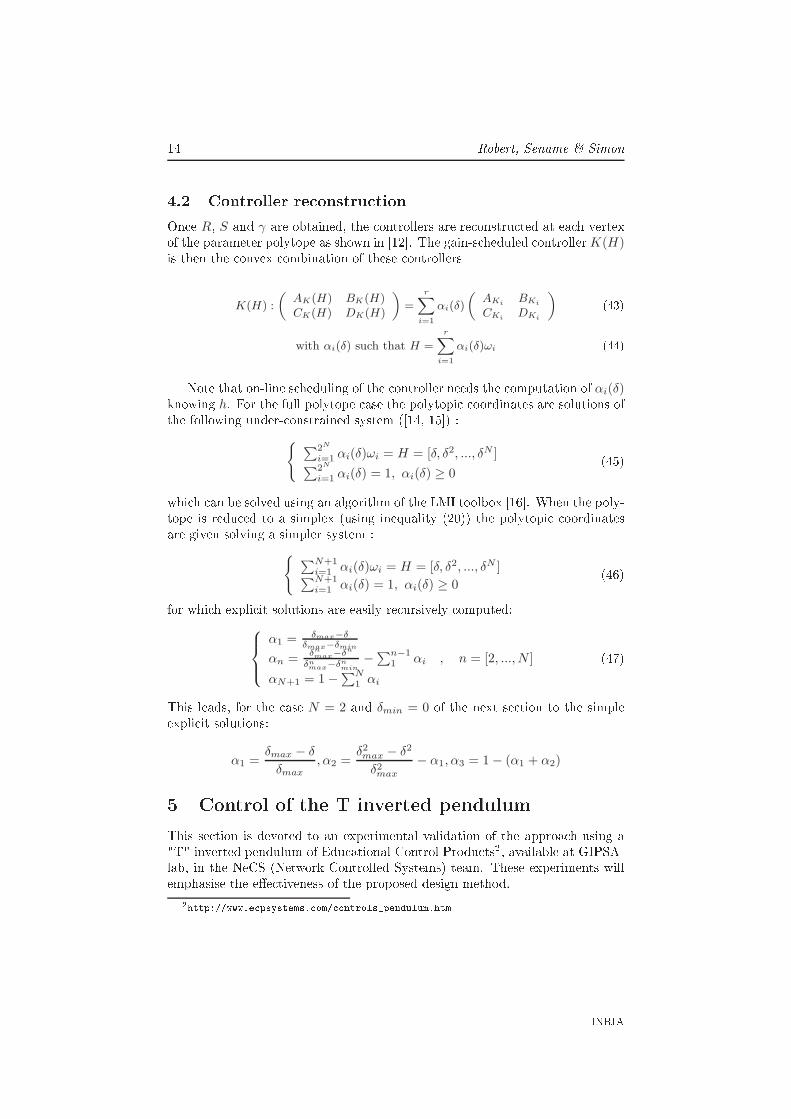
14 Robert, Sename & Simon4.2 Controller re onstru tionOn e R, S and γ are obtained, the ontrollers are re onstru ted at ea h vertexof the parameter polytope as shown in [12℄. The gain-s heduled ontroller K(H)is then the onvex ombination of these ontrollersK(H) :

„

AK(H) BK(H)CK(H) DK(H)

«

=r

X

i=1

αi(δ)

„

AKiBKi

CKiDKi

« (43)with αi(δ) such that H =

rX

i=1

αi(δ)ωi (44)Note that on-line s heduling of the ontroller needs the omputation of αi(δ)knowing h. For the full polytope ase the polytopi oordinates are solutions ofthe following under- onstrained system ([14, 15℄) :{

∑2N

i=1αi(δ)ωi = H = [δ, δ2, ..., δN ]

∑2N

i=1αi(δ) = 1, αi(δ) ≥ 0

(45)whi h an be solved using an algorithm of the LMI toolbox [16℄. When the poly-tope is redu ed to a simplex (using inequality (20)) the polytopi oordinatesare given solving a simpler system :{

∑N+1

i=1αi(δ)ωi = H = [δ, δ2, ..., δN ]

∑N+1

i=1αi(δ) = 1, αi(δ) ≥ 0

(46)for whi h expli it solutions are easily re ursively omputed:

α1 = δmax−δδmax−δmin

αn =δn

max−δn

δnmax−δn

min

−∑n−1

1αi , n = [2, ..., N ]

αN+1 = 1 −∑N

1αi

(47)This leads, for the ase N = 2 and δmin = 0 of the next se tion to the simpleexpli it solutions:α1 =

δmax − δ

δmax

, α2 =δ2max − δ2

δ2max

− α1, α3 = 1 − (α1 + α2)5 Control of the T inverted pendulumThis se tion is devoted to an experimental validation of the approa h using a"T" inverted pendulum of Edu ational Control Produ ts2, available at GIPSA-lab, in the NeCS (Network Controlled Systems) team. These experiments willemphasise the e�e tiveness of the proposed design method.2http://www.e psystems. om/ ontrols_pendulum.htmINRIA

An H∞ LPV Design for Sampling Varying Controllers : Experimentation with a T Inverted Pendulum155.1 System des riptionThe pendulum shown in �gures 6 and 7 is made of two rods. A verti al onewhi h rotates around the pivot axle, and an horizontal sliding balan e one. Twooptional masses allow to modify the plant's dynami al behaviour.The ontrol a tuator (DC motor) delivers a for e u to the horizontal slidingrod, through a drive gear-ra k.The θ angle, positive in the trigonometri sense, is measured by the rod anglesensor. The position z of the horizontal rod is measured by a sensor lo ated atthe motor axle.The DC motor is torque ontrolled using a lo al urrent feedba k loop (as-sumed to be a simple gain due to its fast dynami s). The dynami al behaviourof the sensors is also negle ted.

Figure 6: Pi ture of the T pendulum

θ(t)

z(t)

u(t)

Figure 7: Coordinates of the T pendu-lum5.2 ModellingA me hani al model of the pendulum is presented below, whi h takes into a - ount the vis ous fri tion (but not the Coulomb fri tion).(

m1 m1l0m1l0 J

) (

z

θ

)

+

(

−fvz−m1zθ

2m1zθ 0

) (

z

θ

)

+

(

−m1 sin θ−(m1l0 + m2lc) sin θ − m1z cos θ

)

g =

(

u0

) (48)where the time dependen e of the state variables is impli it, and the parametervalues of given below in table 1.RR n° 6380

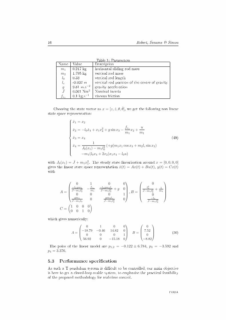
16 Robert, Sename & SimonTable 1: ParametersName Value Des riptionm1 0.217 kg horizontal sliding rod massm2 1.795 kg verti al rod massl0 0.33 verti al rod lengthlc -0.032 m verti al rod position of the entre of gravityg 9.81 m.s−2 gravity a elerationJ 0.061 Nm2 Nominal inertia

fvz0.1 kg.s−1 vis ous fri tionChoosing the state ve tor as x = [z, z, θ, θ], we get the following non linearstate spa e representation:

x1 = x2

x2 = −l0x4 + x1x24 + g sin x3 −

fvz

m1

x2 +u

m1

x3 = x4

x4 =1

J0(x1) − m1l20(+g(m1x1 cosx3 + m2lc sin x3)

−m1(l0x4 + 2x2)x1x4 − l0u)

(49)with J0(x1) = J + m1x

21. The steady-state linearisation around x = [0, 0, 0, 0]gives the linear state spa e representation x(t) = Ax(t) + Bu(t), y(t) = Cx(t)with

A =

0 1 0 0−l0gm1

J−m1l20

−fvz

m1

−l0gm2lcJ−m1l2

0

+ g 0

0 0 0 1gm1

J−m1l00 gm2lc

J−m1l20

0

, B =

0l20

J−m1l20

+ 1

m1

0−l0

J−m1l20

C =

(

1 0 0 00 0 1 0

)whi h gives numeri ally:A =

0

B

B

@

0 1 0 0−18.79 −0.46 14.82 0

0 0 0 156.92 0 −15.18 0

1

C

C

A

B =

0

B

B

@

07.520

−8.82

1

C

C

A

(50)The poles of the linear model are p1,2 = −0.122 ± 6.784, p3 = −3.592 andp4 = 3.376.5.3 Performan e spe i� ationAs su h a T pendulum system is di� ult to be ontrolled, our main obje tiveis here to get a losed-loop stable system, to emphasise the pra ti al feasibilityof the proposed methodology for real-time ontrol. INRIA

An H∞ LPV Design for Sampling Varying Controllers : Experimentation with a T Inverted Pendulum17From previous experiments with this plant the sampling period is assumedto be in the interval [1, 3] ms.The hosen performan e obje tives are represented in �gure 8, where thetra king error and the ontrol input are weighted (as usual in the H∞ method-ology).+

du

+ GKr y

Wu

M

We+

−

θ

e

u

Figure 8: General ontrol on�gurationThis orresponds to the simple mixed sensitivity problem given in (51).∥

∥

∥

∥

We(I − MSyGK1) WeMSyGWuSuK1 WuTu

∥

∥

∥

∥

∞

≤ γ (51)withK =

[

K1 K2

]

M =[

0 0 1 0]

Su = (I − K2G)−1 Sy = (I − GK2)−1

Tu = −K2G(I − K2G)−1 (52)The performan e obje tives are represented by weighting fun tions and may begiven by the usual transfer fun tions [11℄:We(p, f) =

p MS + ωS(f)

p + ωS ǫS

ωS(f) = hmin ωSmaxf (53)

Wu(p, f) =1

MU

(54)where f = 1/h, ωSmax= 1,5 rad/s, MS = 2, ǫS = 0.01 and MU = 5.Noti e that only We depends on the sampling frequen y to a ount for per-forman e adaptation.5.4 Polytopi dis rete-time modelWe follow here the methodology proposed in se tion 2. The approximation isdone around the nominal period ho = 1ms, for h ∈ [1, 3] ms, i.e. δh ∈ [0, 2] ms(see Remark 2).On �gure 9 the riterion (13) is evaluated for di�erent sampling periods(h ∈ [1, 3]ms ) and di�erent orders of the Taylor expansions (k ∈ [1, 5]). Itshows that this error may be large only if the order 1 is used.RR n° 6380

18 Robert, Sename & SimonOn �gure 10 |Gde(δh, z) − Gd(δh, z)| is plotted a ording to the frequen y,evaluated for 5 sampling periods ( i.e. δh ∈ [0, 2]ms) and for two ases of Taylorexpansions (2 and 4). This allows to on lude that the hoi e of an order 2of the Taylor expansion is already quite good as it leads to an approximationerror less than −40dB in the sele ted sampling frequen y interval. Note that hoosing the ase "order 2" leads to a redu ed polytope with 3 verti es.

11.5

22.5

3 12

34

5

10−20

10−15

10−10

10−5

100

105

k

Erreur d’approximation : hinfnorm (Gapprox

−Gd)

h (ms)

Err

eur

Figure 9: Approximation error5.5 LPV/H∞ designThe �rst step is the dis retization of the weighting fun tions. The augmentedsystem is got, using a preliminary �rst-order �ltering of the ontrol input, tosatisfy the design assumptions. The augmented system is of order 6.Applying the design method developed in se tion 4 leads to the following re-sults, ombining the Taylor expansion order and the polytope redu tion:Polytope Nb verti es γoptTaylor order N=2 full 4 1.1304Taylor order N=2 redu ed 3 1.1299Taylor order N=4 full 16 1.1313Taylor order N=4 redu ed 5 1.1303This table emphasises that both design of orders 2 and 4 are reliable. For im-plementation reasons (simpli ity and omputational omplexity) we have hosenthe ase of the redu ed polytope using a Taylor expansion of order 2.The orresponding sensitivity fun tions of the hosen design are shown in �g-ure 11. Using Se = e/r the steady-state tra king error is less than −46dB, witha varying bandwidth from 0.4 to 1.2 rad/s, i.e the ratio 3, spe i�ed a ordingto the interval of sampling period, is satis�ed. INRIA

An H∞ LPV Design for Sampling Varying Controllers : Experimentation with a T Inverted Pendulum19

10−2

100

102

104

−350

−300

−250

−200

−150

−100

−50

0N=2

Mag

nitu

de (

dB)

10−2

100

102

104

−350

−300

−250

−200

−150

−100

−50

0N=4

Frequency (rad/s)

Mag

nitu

de (

dB)

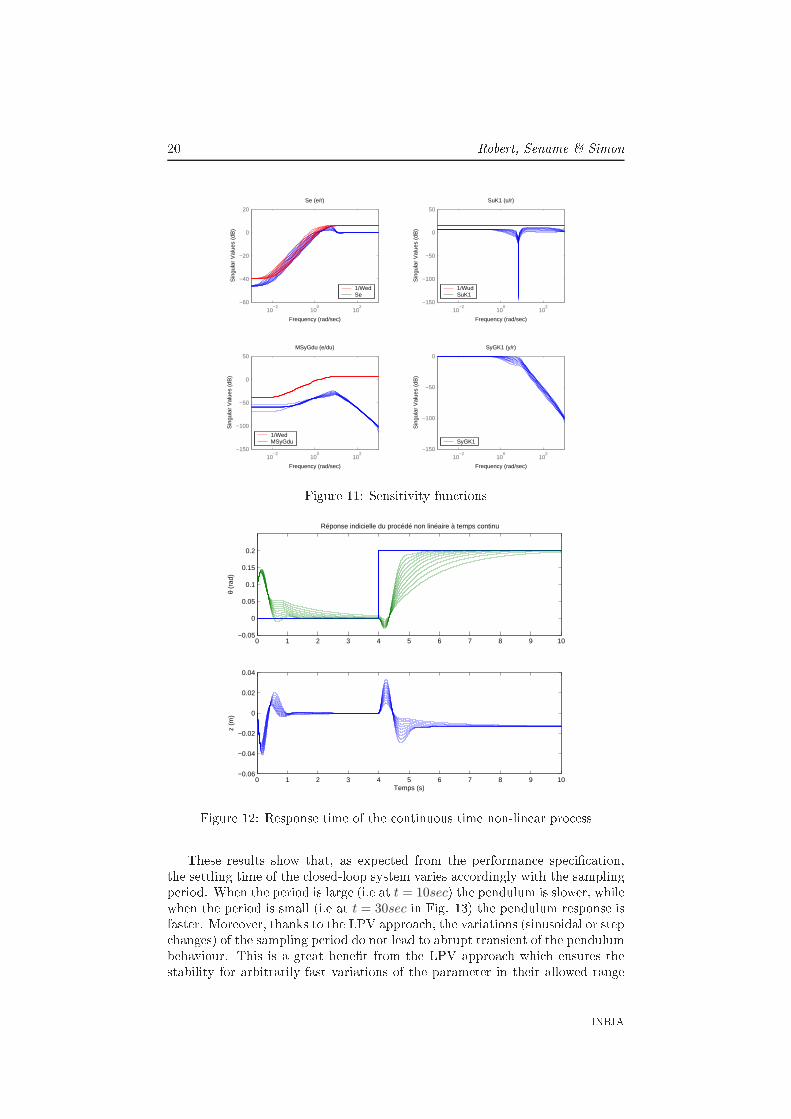
Figure 10: |Gde(δh, z) − Gd(δh, z)| for 6= h - Taylor order 2 and 4The peak value of SuK1 varies from 1.2 to 10.8dB, whi h is reasonable forthe ontrol gain. Note that in this parti ular ase study we will bene�t fromthe relatively high sensitivity in high frequen ies, as it allows some persistentdithering in the ontrol a tion and redu es the e�e t of fri tion, as we will seein the experiments.Finally the fun tion MSyGdu is very low so that the e�e t of input distur-ban e du on the tra king error will be greatly attenuated.Figure 12 shows the time-domain response of the non linear pendulum model(angle and position) inter onne ted with the dis rete-time LPV sampling vari-able ontroller (here for di�erent frozen values of the sampling periods). Thesettling time varies from 1.1 to 4.8 se , i.e. in a ratio 4.3. Indeed we observehere the gra eful and ontrolled degradation of the performan e due to the adap-tion of the sampling dependent weighting fun tions. There is no overshoot, asexpe ted from the frequen y responses of the sensitivity fun tion SyGK1.5.6 Simulation resultsIn this se tion, the appli ation of the proposed sampling variable ontroller whenthe sampling period varies on-line between 1 and 3 mse . is provided.Two ases are presented. First in �gure 13 the sampling period variationis ontinuous and follows a sinusoidal signal of frequen y 0.15rad/s. Then in�gure 14 some step hanges of the sampling period are done.RR n° 6380

20 Robert, Sename & Simon10

−210

010

2−60

−40

−20

0

20

1/WedSe

10−2

100

102

−150

−100

−50

0

50

1/WudSuK1

10−2

100

102

−150

−100

−50

0

50

1/WedMSyGdu

10−2

100

102

−150

−100

−50

0

SyGK1

Se (e/r)

Frequency (rad/sec)

Sin

gula

r V

alue

s (d

B)

SuK1 (u/r)

Frequency (rad/sec)

Sin

gula

r V

alue

s (d

B)

MSyGdu (e/du)

Frequency (rad/sec)

Sin

gula

r V

alue

s (d

B)

SyGK1 (y/r)

Frequency (rad/sec)

Sin

gula

r V

alue

s (d

B)

Figure 11: Sensitivity fun tions0 1 2 3 4 5 6 7 8 9 10

−0.05

0

0.05

0.1

0.15

0.2

θ (r

ad)

Réponse indicielle du procédé non linéaire à temps continu

0 1 2 3 4 5 6 7 8 9 10−0.06

−0.04

−0.02

0

0.02

0.04

z (m

)

Temps (s)Figure 12: Response time of the ontinuous time non-linear pro essThese results show that, as expe ted from the performan e spe i� ation,the settling time of the losed-loop system varies a ordingly with the samplingperiod. When the period is large (i.e at t = 10sec) the pendulum is slower, whilewhen the period is small (i.e at t = 30sec in Fig. 13) the pendulum response isfaster. Moreover, thanks to the LPV approa h, the variations (sinusoidal or step hanges) of the sampling period do not lead to abrupt transient of the pendulumbehaviour. This is a great bene�t from the LPV approa h whi h ensures thestability for arbitrarily fast variations of the parameter in their allowed rangeINRIA

An H∞ LPV Design for Sampling Varying Controllers : Experimentation with a T Inverted Pendulum21(this is due to the use of a single Lyapunov fun tion in the design [7℄). Thesame assessment an be done for the ontrol input.The LPV s heme allows here to guarantee the losed-loop quadrati stability,to have a bounded L2-indu ed norm for all variation of the sampling period andto have a predi table losed-loop behaviour.0 10 20 30 40 50 60 70 80 90

−0.4

−0.2

0

0.2

0.4Angle du pendule

θ [r

ad]

rθ

0 10 20 30 40 50 60 70 80 90−2

−1

0

1

2

u []

Commande

0 10 20 30 40 50 60 70 80 901

1.5

2

2.5

3x 10

−3

h [s

]

Période d’échantillonnage

Temps [s]Figure 13: Motion of the T pendulum under a sinusoidal sampling period0 10 20 30 40 50 60 70 80 90

−0.4

−0.2

0

0.2

0.4Angle du pendule

θ [r

ad]

rθ

0 10 20 30 40 50 60 70 80 90−2

−1

0

1

2

u []

Commande

0 10 20 30 40 50 60 70 80 900

1

2

3

4x 10

−3

h [s

]

Période d’échantillonnage

Temps [s]Figure 14: Motion of the T pendulum under a square sampling periodRR n° 6380

22 Robert, Sename & Simon5.7 ExperimentsThe s enarii of the previous se tion (simulation results) are now implementedfor the real plant of �gure 6. The plant is ontrolled through Matlab/Simulinkusing the Real-time Workshop and xPC Target.0 10 20 30 40 50 60 70 80 90

−0.5

0

0.5

θ [r

ad]

Pendulum angle

0 10 20 30 40 50 60 70 80 90−4

−2

0

2

4

u []

Control input

0 10 20 30 40 50 60 70 80 901

1.5

2

2.5

3x 10

−3

Time [s]

h [s

]

Sampling period

rθ

u

h

Figure 15: Experimental motion of the T pendulum under a sinusoidal samplingperiod0 10 20 30 40 50 60 70 80 90

−0.5

0

0.5

θ [r

ad]

Pendulum angle

0 10 20 30 40 50 60 70 80 90−5

0

5

u []

Control input

0 10 20 30 40 50 60 70 80 900

1

2

3

4x 10

−3

Time [s]

h [s

]

h

u

rθ

Figure 16: Experimental motion of the T pendulum under a square samplingperiod INRIA

An H∞ LPV Design for Sampling Varying Controllers : Experimentation with a T Inverted Pendulum23The results are given in �gures 15 and 16. As in the previous se tion, thesettling time is maximal when the sampling period is maximal, and onversely.In the same way, there is no abrupt hanges in the ontrol input (even when thesampling period abruptly varies from 1 to 3 ms as in �gure 16).Note that, as explained before, the real ontrol input is sensitive to noise,allowing to minimise the fri tion e�e t, and therefore to obtain a losed-loopsystem with mu h less os illations.Finally we get similar results in simulation and experimental tests whi hshows the inherent robustness property of the H∞ design.These results emphasise the great advantage and �exibility of the methodwhen the available omputing resour es may vary, and when sampling periodvariations are used to handle omputing �exibility su h as in [4℄.6 Con lusionIn this paper, an LPV approa h is proposed to design a dis rete-time linear ontroller with a varying sampling period and varying performan es. A way toredu e the polytope from 2N to N + 1 verti es (where N is the Taylor orderexpansion) is provided, whi h drasti ally redu es both the onservatism and the omplexity of the resulting sampling dependent ontroller and makes the solu-tion easier to implement. Further developments may on ern the redu tion ofthe onservatism whi h is due to to the use a onstant Lyapunov fun tion ap-proa h, whi h is known to produ e a sub-optimal ontroller. Another approa hbased on [17℄ is presented in [13℄ but up to now did not give improvements inthe results.Also the omplete methodology has been implemented for the ase of a"T" inverted pendulum, where experimental results have been provided. Theseresults emphasise the real e�e tiveness of the LPV approa h as well as its interestin the ontext of adaptation to varying pro essor or network load where a bank ofswit hing ontrollers would need too mu h resour es. In our ase, using a single ontroller synthesis, the stability and performan e property of the losed-loopsystem are guaranteed whatever the speed of variations of the sampling periodare. In addition we also observed an interesting robustness of this ontrollerw.r.t. sampling ina ura ies, e.g. whi h ould be indu ed by preemptions in amulti-tasking operating systems. As shown in preliminary studies ([4, 13℄), theseproperties are of prime interest in the design of more omplex systems ombiningseveral su h ontrollers under supervision of a feedba k-s heduler : the ontrolperiods an be varied arbitrarily fast by an outer s heduling loop under a QoSobje tive with no risk of jeopardising the plants stability. However the spe i� robustness w.r.t. timing un ertainties deserve to be further investigated.Referen es[1℄ A. Cervin and J. Eker, �Feedba k s heduling of ontrol tasks,� in Pro- eedings of the 39th IEEE Conferen e on De ision and Control, Sydney,Australia, De . 2000.RR n° 6380

24 Robert, Sename & Simon[2℄ A. Cervin, J. Eker, B. Bernhardsson, and K.-E. Årzén, �Feedba k-feedforward s heduling of ontrol tasks,� Real-Time Systems, vol. 23, no.1�2, pp. 25�53, July 2002.[3℄ J. Eker, P. Hagander, and K.-E. Årzén, �A feedba k s heduler for real-time ontroller tasks,� Control Engineering Pra ti e, vol. 8, no. 12, pp. 1369�1378, De . 2000.[4℄ D. Simon, D. Robert, and O. Sename, �Robust ontrol/s heduling o-design: appli ation to robot ontrol,� in RTAS'05 IEEE Real-Time andEmbedded Te hnology and Appli ations Symposium, San Fran is o, mar h2005.[5℄ D. Robert, O. Sename, and D. Simon, �Sampling period dependent rst ontroller used in ontrol/s heduling o-design,� in Pro eedings of the 16 thIFAC World Congress, Cze h Republi , July 2005.[6℄ ��, �Synthesis of a sampling period dependent ontroller using LPV ap-proa h,� in 5th IFAC Symposium on Robust Control Design ROCOND'06,Toulouse, Fran e, july 2006.[7℄ P. Apkarian, P. Gahinet, and G. Be ker, �Self-s heduled H∞ ontrol oflinear parameter-varying systems: A design example,� Automati a, vol. 31,no. 9, pp. 1251�1262, 1995.[8℄ K. Tan, K.-M. Grigoriadis, and F. Wu, �Output-feedba k ontrol of LPVsampled-data systems,� Int. Journal of Control, vol. 75, no. 4, pp. 252�264,2002.[9℄ K. J. Åström and B. Wittenmark, Computer-Controlled Systems, 3rd ed.,ser. Information and systems s ien es series. New Jersey: Prenti e Hall,1997.[10℄ S. Boyd and L. Vandenberghe, Convex Optimization. Cambridge Univer-sity Press, 2004.[11℄ S. Skogestad and I. Postlethwaite, Multivariable Feedba k Control: analysisand design. John Wiley and Sons, 1996.[12℄ P. Gahinet and P. Apkarian, �A linear matrix inequality approa h to h∞ ontrol,� International Journal of Robust and Nonlinear Control, vol. 4, pp.421�448, 1994.[13℄ D. Robert, �Contribution to ontrol and s heduling intera tion,� Ph.D. dis-sertation, INPG - Laboratoire d'Automatique de Grenoble (in fren h), jan-uary 11, 2007.[14℄ J.-M. Bianni , �Commande robuste des systèmes à paramètres variables,�Ph.D. dissertation, ENSAE, Toulouse, Fran e, 1996.[15℄ A. Zin, �On robust ontrol of vehi le suspensions with a view to global hassis ontrol,� Ph.D. dissertation, INPG - Laboratoire d'Automatique deGrenoble, november 3, 2005. INRIA

An H∞ LPV Design for Sampling Varying Controllers : Experimentation with a T Inverted Pendulum25[16℄ P. Gahinet, �Expli it ontroller formulas for LMI-based H∞ synthesis,�Automati a, vol. 32, no. 7, pp. 1007�14, 1996.[17℄ M. Oliveira, J. Geromel, and J. Bernussou, �Extended h2 and hinf norm hara terizations and ontroller parametrizations for dis rete-time sys-tems,� International Journal of Control, vol. 75, no. 9, pp. 666�679, 2002.

RR n° 6380

Centre de recherche INRIA Grenoble – Rhône-Alpes655, avenue de l’Europe - 38334 Montbonnot Saint-Ismier (France)

Centre de recherche INRIA Futurs : Parc Orsay Université - ZAC des Vignes4, rue Jacques Monod - 91893 ORSAY Cedex

Centre de recherche INRIA Nancy – Grand Est : LORIA, Technopôle de Nancy-Brabois - Campus scientifique615, rue du Jardin Botanique - BP 101 - 54602 Villers-lès-Nancy Cedex

Centre de recherche INRIA Rennes – Bretagne Atlantique : IRISA, Campus universitaire de Beaulieu - 35042 Rennes CedexCentre de recherche INRIA Paris – Rocquencourt : Domaine de Voluceau - Rocquencourt - BP 105 - 78153 Le Chesnay CedexCentre de recherche INRIA Sophia Antipolis – Méditerranée :2004, route des Lucioles - BP 93 - 06902 Sophia Antipolis Cedex

ÉditeurINRIA - Domaine de Voluceau - Rocquencourt, BP 105 - 78153 Le Chesnay Cedex (France)http://www.inria.fr

ISSN 0249-6399