hal.inria.fr · hal id: hal-00695799 submitted on 9 may 2012 hal is a multi-disciplinary open...
TRANSCRIPT

HAL Id: hal-00695799https://hal.inria.fr/hal-00695799
Submitted on 9 May 2012
HAL is a multi-disciplinary open accessarchive for the deposit and dissemination of sci-entific research documents, whether they are pub-lished or not. The documents may come fromteaching and research institutions in France orabroad, or from public or private research centers.
L’archive ouverte pluridisciplinaire HAL, estdestinée au dépôt et à la diffusion de documentsscientifiques de niveau recherche, publiés ou non,émanant des établissements d’enseignement et derecherche français ou étrangers, des laboratoirespublics ou privés.
Liquid and liquid-gas flows at all speeds : Referencesolutions and numerical schemes
Sebastien Lemartelot, Boniface Nkonga, Richard Saurel
To cite this version:Sebastien Lemartelot, Boniface Nkonga, Richard Saurel. Liquid and liquid-gas flows at all speeds :Reference solutions and numerical schemes. Journal of Computational Physics, Elsevier, 2012, 66,pp.62-78. 10.1016. hal-00695799

ISS
N0
24
9-6
39
9IS
RN
INR
IA/R
R--
79
35
--F
R+
EN
G
RESEARCH
REPORT
N° 7935Avril 2012
Project-Teams SMASH etPUMAS
Liquid and liquid-gas
flows at all speeds :
Reference solutions and
numerical schemes
S. LeMartelot , B. Nkonga , R. Saurel


RESEARCH CENTRE
SOPHIA ANTIPOLIS – MÉDITERRANÉE
2004 route des Lucioles - BP 93
06902 Sophia Antipolis Cedex
Liquid and liquid-gas flows at all speeds :
Reference solutions and numerical schemes
S. LeMartelot ∗, B. Nkonga †, R. Saurel ‡
Project-Teams SMASH et PUMAS
Research Report n° 7935 — Avril 2012 — 61 pages
∗ Polytech’Marseille, Aix-Marseille University, UMR CNRS 6595 IUSTI, 5 rue E. Fermi, 13453 Marseille Cedex
13, France† University of Nice, LJAD UMR CNRS 7351, Parc Valrose, 06108 Nice Cedex, INRIA Sophia-Antipolis‡ Polytech’Marseille, Aix-Marseille University, UMR CNRS 6595 IUSTI, 5 rue E. Fermi, 13453 Marseille Cedex
13, France, INRIA Sophia-Antipolis

Abstract: All speed flows and in particular low Mach number flow algorithms are addressedfor the numerical approximation of the Kapila et al. [19] multiphase flow model. This model isvalid for fluid mixtures evolving in mechanical equilibrium but out of temperature equilibrium andis efficient for material interfaces computation separating miscible and non-miscible fluids. In thiscontext, the interface is considered as a numerically diffused zone, captured as well as all presentwaves (shocks, expansion waves). The same flow model can be used to solve cavitating and boilingflows [39]. Many applications occurring with liquid-gas interfaces and cavitating flows involve avery wide range of Mach number variations, from 10−3 to 100 with respect to the mixture soundspeed. It is thus important to address numerical methods free of restrictions regarding the Machnumber.To assess the accuracy of such schemes, reference solutions are needed and there is a clear lackin this domain. We address here exact one-dimensional liquid and liquid-gas compressible flowssolutions in nozzles. The exact solution is first derived for the compressible single liquid phase Eulerequations and extends the well known ideal gas dynamic nozzle flow solutions. This referencesolution is then extended to the Kapila et al. [19] model that contains two entropies and nonconventional shock relations. The all Mach number scheme is then derived. A preconditionedRiemann solver is built and embedded into the Godunov explicit scheme. It is shown that thismethod converges to exact solutions but needs too small time steps to be efficient. An implicitversion is then derived, in one dimension first and second in the frame of 3D unstructured meshes.Two-phase flow preconditioning is then addressed in the frame of the Saurel et al [38] algorithm.Modifications of the preconditioned Riemann solver are needed and detailed. Convergence of bothsingle phase and two-phase numerical solutions are demonstrated with the help of exact ones. Last,the method is illustrated by the computation of real cavitating flows in Venturi nozzles. Vaporpocket size and instability frequencies are perfectly reproduced by the model and method withoutusing any parameters. In particular, no turbulence model is used.
Key-words: hyperbolic systems, multifluid, multiphase, Venturi, cavitation, preconditioned,unstructured meshes, HLLC.

Liquid and liquid-gas flows at all speeds :
Reference solutions and numerical schemes
Résumé :
Mots-clés :

4 S. LeMartelot, B. Nkonga and R. Saurel
1 Introduction
Liquid-gas mixtures and interfacial flows arise in many natural and industrial situations occur-ring in fluid mechanics, nuclear, environmental and chemical engineering. Most computationalapproaches consider the two fluids as incompressible (Hirt and Nichols [17], Lafaurie et al [22],Menard et al [24]) to cite a few. High Mach number flows with material interfaces have alsobeen the subject of important efforts, with various approaches: Front Tracking [11], Level Setand Ghost Fluid [10], diffuse interfaces [1], [34], [38] and others. Only a few works deal withincompressible liquid and compressible gas [18]. However, in many applications gas compressibil-ity is of paramount importance as, for example, when phase change occurs. In cavitating flows,compressibility of all phases is important as the liquid phase change occurs under liquid expan-sion effects. Moreover, when liquid-gas mixtures appear, the sound propagates with the mixturesound speed [45] that has a non monotonic behaviour with respect to the volume fraction, result-ing in very low sound speed, of the order of a few meters per second. There is thus no difficulty toreach hypersonic flow conditions with liquid gas mixtures. Consequently, it is important to buildnumerical methods able to deal with incompressible flows, transonic flows and even hypersonicflows in the presence of wave dynamics. This issue has been addressed intensively in the contextof single phase flows since Harlow and Amsden [15] extending incompressible flow solvers to com-pressible flows and Turkel [43] extending compressible flow solvers to the incompressible limit.For now, it seems that multiphase flows in the low Mach regime has been addressed more bymethods issued of incompressible flows. However, this poses difficulties when wave dynamics ispresent, as incompressible flow solvers are not conservative in the compressible flow sense. Also,these methods have difficulties when large density ratios are present. At liquid gas interfaces,the density ratio may exceed several thousands.In the present work we consider liquid-gas interfaces as diffuse numerical zones and adopt theKapila et al. [19] model. This has some advantages:- The interfaces are handled routinely, as any point of the flow.- The dynamic appearance of interfaces (not present initially) is possible thanks to the volumefraction equation structure that allows volume fraction growth in zones where the velocity di-vergence is non zero. This occurs typically in expansion and compression waves and is of majorimportance in cavitating flows.- The phases mass, mixture momentum and mixture energy are expressed under conservativeform, insuring correct wave dynamics in pure fluids zones.- The addition of surface tension [29] as well as phase transition [39] can be done quite easily ina thermodynamically consistent way. In other words, capillary effects are modeled with the helpof a capillary tensor that enters in the momentum and energy fluxes conservatively. The entropyis also preserved. When phase transition is considered, the model guarantees mixture entropyproduction.This approach has obviously some drawbacks:- The interfaces can be excessively diffused, especially when dealing with long time evolutions.But this is exactly the same drawback as contact discontinuity smearing in gas dynamics compu-tations. Efforts to reduce numerical diffusion have been done recently by Kokh and Lagoutière[21] and Shuckla et al. [41].- Non-conservative equations are present and the numerical approximation of non-conservativeterms poses difficulties in the presence of shocks [36], [30], [38], [32].- The building of all Mach number method for this kind of hyperbolic flow model is not an easytask, as will be shown latter.As the flow model is conservative regarding the phases mass equations, mixture momentum andmixture energy and since the system is hyperbolic we will follow a method issued from compress-
Liquid and liquid-gas flows at all speeds 5
ible flow dynamics [43]. This choice is motivated by the importance of the pressure waves presentin many applications, the presence of huge density ratios at interfaces, that are easier to handlewith discontinuity capturing schemes and by the presence of huge Mach number variations. Forspecific applications, this is mandatory as for example with:- liquid-gas flows in nozzle and Venturi tunnels,- high performance turbopumps where cavitation appears,- propellers,- water waves breaking,- flash vaporization.The first difficulty with the design of a numerical scheme is related to its convergence. This posesthe question of reference solutions. Most low Mach number methods predictions are comparedagainst multidimensional flow solutions, typically around airfoils, under the assumption of po-tential flows. We believe it is simpler and more efficient to address one-dimensional flows. In thisaim, liquid nozzle flow solution is determined in the context of the Euler equations and stiffenedgas equation of state (SG EOS). This extends the well known ideal gas nozzle flow solutions.In the low Mach regime, the exact compressible solution is compared to the incompressible one,showing excellent agreement. This reference solution allows immediate comparison of conven-tional hyperbolic flow solvers in this limit. It is shown that conventional methods (Godunov typefor example) result in several orders of magnitude errors in the pressure computation. We thenaddress liquid-gas nozzle flow solution for the Kapila et al. [19] model, again for fluids governedby the SG EOS. The single phase exact solution is extended to the two-phase case with the helpof multiphase shock relations [35]. Thanks to these reference solutions, we then address all Machnumber schemes building in the frame of Turkel [43] formulation.From theoretical standpoint, mathematical analysis of the low Mach number limit for classi-cal solutions of the compressible Navier-Stokes has been investigated by many authors (Ebin[8] , Klainerman and Majda [20], Schochet [40], Metivier and Schochet [26], and many others).Alazard [2] proved, in a rigorous analysis and general context, the existence of uniformly boundedincompressible limit of the full Navier-Stokes equations. The existence time is there independentof the Mach, the Reynolds and the Peclet numbers and thereby includes the limit for the Eulerequation as well. On this theoretical basis, we first consider the single phase Euler equationsand derive an approximate preconditioned Riemann solver. When the Godunov scheme is usedwith this Riemann solver, convergence to the exact nozzle flow solution is obtained. However,the method requires too small time steps (much smaller that the conventional CFL restriction)to be stable. We thus consider implicit formulation to overcome this restriction. The HLLC fluxof Toro et al. [42] is considered and a Taylor expansion is done to express its time variation.The method is first presented in the context of the one-dimensional Euler equations and thenextended to the one-dimensional Kapila et al. [19] model. After validation against the exactone-dimensional two-phase nozzle flow solution, 3D extension of the algorithm for unstructuredmeshes is presented. Computational examples are shown in 3D. In particular, a real cavitatingflow in 3D Venturi channel is examined. With the help of the new method, perfect agreementwith the measured cavitation pocket size and detachment frequency is obtained without havingrecourse to any model or method parameter.The paper is organized as follows. In Section 2 the various flow models under interest are pre-sented: the Euler equations, the Kapila et al. [19] model, the pressure non-equilibrium model ofSaurel et al. [38] that is used to solve the non-conservative pressure equilibrium model of Kapilaet al. [19]. In Section 3, the exact liquid one-dimensional nozzle flow solution is detailed. It isthen extented to two-phase liquid-gas flows. In Section 4 the low Mach single phase Riemannsolver is presented. It uses the preconditioned Euler equations in the Riemann problem resolu-tion only, while the conventional conservative formulation is used for the solution update. Its

6 S. LeMartelot, B. Nkonga and R. Saurel
extension to the two-phase flow model is then examined. To overcome the stability restriction ofthese methods, the implicit formulation of the Godunov method is given in 1D in the context ofthe Euler equations, with the HLLC Riemann solver and preconditioned formulation. Methodconvergence to the exact solution is demonstrated in both low and high Mach conditions. Thetwo-phase flows extension on the basis of the pressure relaxation model of Saurel et al. [38]is then addressed, in one-dimension again. Convergence to the exact two-phase solution andthree dimensional extension of the algorithm for multiphase flows are addressed in the samesection. Computational example and validations against experimental data are given in section5. Conclusions are given in Section 6.
2 Flow Models
In the present study, we are going to consider various flow models, single and two-phase. Thesingle phase one correspond to the Euler equations:
∂ρ
∂t+ div (ρu) = 0
∂ρu
∂t+ div (ρu ⊗ u + P ) = 0
∂ρE
∂t+ div ((ρE + P )u) = 0
(1)
where ρ is the density, u is the velocity vector, P is the pressure, E is the total energy, withE = e + 1
2u2, whith e the internal energy. The thermodynamic closure is achieved by a convex
EOS: P = P (ρ, e). In the present work the SG EOS [14] [25] is used:
p = (γ − 1)ρe− γP∞ (2)
γ and P∞ are parameters of the EOS, obtained from reference thermodynamic curves, charac-teristic of the material and transformation under study. See Le Metayer et al (2004) [27] fordetails.
The two phase flow model we will consider is the one of Kapila et al (2001) [19]. It describesmultiphase mixtures evolving in mechanical equilibrium (equal pressures and equal velocities).It is particularly suited to materials interfaces computations, considered as numerical diffusionzones (see for example Saurel et al [38])
∂α1
∂t+ u • grad (α1) = Kdiv (u)
∂α1ρ1
∂t+ div (α1ρ1u) = 0
∂α2ρ2
∂t+ div (α2ρ2u) = 0
∂ρu
∂t+ div (ρu ⊗ u + P ) = 0
∂ρE
∂t+ div ((ρE + P )u) = 0
where K =ρ2c
22 − ρ1c
21
ρ1c2
1
α1
+ρ2c
2
2
α2
(3)
ck represents the sound speed defined by c2k = ∂pk
∂ρk
)
sk, k = 1, 2,
P represents the mixture pressure,E represents mixture total energy,αk represent the phases volume fraction,ρk represent the phase densities.

Liquid and liquid-gas flows at all speeds 7
Model’s thermodynamic closure is achieved with the help of the mixture energy definition:
ρe = α1ρ1e1 + α2ρ2e2
and the pressure equilibrium condition: p1 = p2. In the context of fluids governed by the SGEOS (2), the mixture EOS reads:
P =
ρe− (α1γ1P∞,1
γ1 − 1+
α2γ2P∞,2
γ2 − 1)
α1
γ1 − 1+
α2
γ2 − 1
(4)
The numerical approximation of the Kapila et al. [19] model is addressed in the frame of Godunovtype finite volume schemes. These schemes are appropriate for non linear hyperbolic equationsand proceed with a transport step achieved with the help of appropriate Riemann solvers anda projection step based on cell averages and thermodynamic computations. To overcome thedifficulties related to the approximation of the non conservative term Kdiv(u) in the volumefraction equation of System (3) a pressure non equilibrium system (5) is considered during thetransport step and a proper projection is achieved to recover the target model (3). The pressurenon equilibrium system reads:
∂α1
∂t+ u • grad (α1) = µ(p1 − p2)
∂α1ρ1
∂t+ div (α1ρ1u) = 0
∂α2ρ2
∂t+ div (α2ρ2u) = 0
∂α1ρ1e1
∂t+ div (α1ρ1e1u) + α1p1div (u) = −pIµ(p1 − p2)
∂α2ρ2e2
∂t+ div (α2ρ2e2u) + α2p2div (u) = pIµ(p1 − p2)
∂ρu
∂t+ div (ρu ⊗ u + P ) = 0
∂ρE
∂t+ div ((ρE + P )u) = 0
(5)
Whereµ represents the pressure relaxation coefficient,
pI represents the interfacial pressure defined by pI =Z1p2 + Z2p1
Z1 + Z2,
with Zk = ρkck, the phase k acoustic impedance.ek and pk represent the phase k internal energy and pressure respectively.
It is important to note that in this system the internal energies of each phase are independentvariables and their evolution is described by two additional equations. The mixture pressure isnow related to the phases’ internal energies:
P = α1p1 + α2p2 (6)
where p1 = p1(ρ1, e1) and p2 = p2(ρ2, e2)
The non equilibrium system (5) is hyperbolic and appropriate to overcome the difficulties related

8 S. LeMartelot, B. Nkonga and R. Saurel
to the discretisation of the volume fraction, in particular regarding positiveness issues. System(5) is used to reach solutions of System (3) in the limit of infinite pressure relaxation, i.e. whenµ tends to infinity.It is worth to mention that System (5) is overdetermined. Indeed, the total energy equation isa consequence of the phases energy equations and the mixture momentum one. This overde-termination will be used to correct the inacuracy appearing during the numerical integration ofαkpkdiv(u), the non conservative terms of the internal energy equations [38]. Overdeterminedsystems have already been considered for numerical approximation issues in different contextsby Babii et al. [3] for example.To be more precise, each integration time step is structured as follows [38]:
- Initialization: At a given time step, the flow is in mechanical equilibrium, in particular inpressure equilibrium. The set of variables is given by:
(αn1 , ρ
n1 , ρ
n2 , u
n, en1 (ρn1 , p
n), en2 (ρn2 , p
n), En)
- Non equilibrium evolution: The pressure relaxation terms are removed (µ = 0) and thehyperbolic pressure non equilibrium system (5) is solved. At the end of this evolution stepa temporary flow state is determined, out of pressure equilibrium:
(αn+11 , ρn+1
1 , ρn+12 , un+1, en+1
1 , en+12 , En+1)
- Projection to pressure equilibrium: This step deals with the projection of the previouspressure non equilibrium state onto a pressure equilibrium one:
(αn+11 , ρn+1
1 , ρn+12 , un+1, en+1
1 (ρn+11 , pn+1), en+1
2 (ρn+12 , pn+1), En+1)
This is done by determining the asymptotic solution of the remaining relaxation ODE system inthe limit µ → +∞.The asymptotic state is determined by the resolution of a non linear algebraicequation. Details may be found, for example, in [38].It is worth to mention that:
- The equilibrium pressure pn+1 is determined from the mixture EOS (4), based on the mixturetotal energy En+1, for which there is no conservation issue.
- Both steps in this strategy preserves volume fraction positivity.
- Both steps preserve phases’ mass conservation, mixture momentum and energy conservation.
- The entropy inequality is also preserved during each step.
This algorithm has shown robustness, accuracy and versatility for various flow models rang-ing from interfaces, supercavitating flows [39], detonation waves [31], powder compaction [37],solid-fluid coupling [9] in severe high speed conditions. We address here arbitrary velocity flowconditions and particularly low Mach number conditions.The first issue in this frame is related to the determination of reference solutions to check methodconvergence and improve existing schemes in arbitrary flow conditions. This issue is addressedin the next section for single and two-phase steady flows in nozzles and Venturi ducts.

Liquid and liquid-gas flows at all speeds 9
3 Reference solutions
The aim is to determine the one dimensional two phase nozzle flow solution of System (3) forfluids governed by the SG EOS (2). For the sake of simplicity in the presentation, we first detailthe exact solution for single phase liquid flows governed by the Euler equations (System 1) andSG EOS (2). We then extend the solution method determination to the two-phase nozzle flowcontext.
3.1 Single phase nozzle flow
In this section, the single phase exact solution determination is addressed. To do so, we considera nozzle connected to a tank at left and opened to the atmosphere at the right outlet, as shownin the Figure 1. The tank state is denoted by subscript "0" while the outlet state is denoted by
Figure 1: Nozzle connected to a tank at the inlet and to a prescribed pressure at the outlet
subscript "out". The tank state is defined by :
W0 =
ρ0u0
p0
Where ρ0 and p0 are prescribed density and pressure respectively and u0 = 0. In order todetermine the nozzle flow solution, it is first necessary to determine the flow configuration. Itcan be subsonic everywhere, supersonic in the divergent, supersonic with a shock in the divergent.All theses configurations have to be considered. To do so, various critical pressure ratios have tobe determined.
3.1.1 Critical pressure ratios
The first critical pressure ratio corresponds to the appearance of a sonic state throath. Obviously,for liquids, such sonic state requires very high pressure ratios. But, as shown later, such statecan be reached with moderate pressure ratios when dealing with two phase mixtures.
Critical pressure ratio 1 (cpr1) The critical pressure ratio, cpr1, is defined as the out-let/tank pressure ratio corresponding to a subsonic flow everywhere except at the throat wherechocking conditions (u = c) appear.As the flow is isentropic everywhere, the following relations are used:
H∗ = H0 and s∗ = s0 (7)
Where:s represents the entropy
H represents the total enthalpy, defined by H = e+p
ρ+
1
2u2
The "*" superscript represents the nozzle throat state for which u∗ = c∗.

10 S. LeMartelot, B. Nkonga and R. Saurel
Using the SG EOS, relations (7) become:
γ (p∗ + P∞)
(γ − 1) ρ∗+
1
2u∗2 = H0 and
p∗ + P∞
ρ∗γ=
p0 + P∞
ργ0
(8)
The last unknown is the velocity at the nozzle throat, u∗.The SG EOS sound speed reads :
c =
√
γp+ P∞
ρ(9)
As, u∗ = c∗, combining relation (8) and (9) yields the throat pressure, p∗ :
p∗ + P∞ = (p0 + P∞)(γ + 1
2)
γ − 1
γ (10)
As the critical pressure, p∗, is known, the complete critical state W ∗ is determined with the helpof relations (8).It is necessary to determine the state in the outlet section. Relations (8) can be used again as :
γ (pout + P∞)
(γ − 1) ρout+
1
2Uout = H0 and
pout + P∞
ργ1
=p0 + P∞
ργ0
(11)
The closure relation now corresponds to the mass conservation between the throat section andthe outlet.
Pout = ρoutUoutAo = ρ∗u∗A∗ = m∗ (12)
where Ao represents the outlet section area and A∗ the nozzle throat section area.Using equation (11), the density in the outlet section can be expressed as a function of pout only.Thus, the following expression is obtained for the velocity in the outlet section Uout:
Uout =m∗
ρout(pout)Ao
with ρout = ρ0
(
pout + P∞
p0 + P∞
)
1
γ (13)
Combining relations (13) and (11), a non-linear function of pout is obtained:
γ (pout + P∞)
(γ − 1) ρout(pout)+
1
2
(
m∗
ρout(po)Ao
)2
−H∗ = 0 (14)
This equation admits two roots : pout = pcpr1 and pout = pcpr3.The subsonic branch corresponds to the pressure ratio cpr1. To determine it, the Newton methodis used with initial guess for the outlet pressure pout = p∗. Then, cpr1 is defined as cpr1 =pcpr1 + P∞
p0 + P∞.
Critical pressure ratio 3 (cpr3) This solution corresponds to the supersonic branch of equa-tion (14). Is is obtained again from (14) with the Newton method by taking the initial pressureguess pout = (1 + 10−6)P∞. When convergence is reached, the outlet pressure is determined as
pout = pcpr3. The critical pressure ratio cpr3 is obtained as cpr3 =pcpr3 + P∞
p0 + P∞.

Liquid and liquid-gas flows at all speeds 11
Critical pressure ratio 2 (cpr2) The critical pressure ratio, cpr2, corresponds to a supersonicflow in the nozzle divergent except at the outlet section where a steady shock is present.The flow entering the shock has precisely the state corresponding to Wcpr3. The shocked stateis obtained with the help of the Rankine-Hugoniot relations :
(ρu)cpr3 = (ρu)cpr2 (15)
(
ρu2 + p)
cpr3=(
ρu2 + p)
cpr2(16)
ecpr2 − ecpr3 +pcpr2 + pcpr3
2(vcpr2 − vcpr3) = 0 (17)
With the help of the SG EOS , Equation (17) becomes:
vcpr2
vcpr3= Q (pcpr2, pcpr3) =
(γ − 1)(pcpr2 + P∞) + (γ + 1)(pcpr3 + P∞)
(γ − 1)(pcpr3 + P∞) + (γ + 1)(pcpr2 + P∞)(18)
where v represents the specific volume, v =1
ρ.
Combining relations (18), (15) and (16), a non-linear function of pcpr2 is obtained:
pcpr3 − pcpr2 + ρcpr3 (uc3)2(1−Q (pcpr2, pcpr3)) = 0 (19)
Again, the Newton method is used to determine pcpr2.The initial pressure guess in the Newton method is pcpr2 = pcpr1, as pcpr1 > pcpr2 > pcpr3.
3.1.2 Derivation of the Nozzle flow profile : Single phase Isentropic
When the pressure ration PR =pout + P∞
p0 + P∞is either greater than cpr1 or lower than cpr2, the
flow is isentropic all over the nozzle. As the outlet pressure is given, we can computed theremaining variables at this section. Indeed, the second relation of (8) expressed between thetank and the outlet gives the outlet density :
ρout = ρ0
(
pout + P∞
p0 + P∞
)
1
γ (20)
The outlet velocity is obtained from the first relation in equation (8) appied to the outlet section:
Uout =
√
2
[
H0 −γ(pout + P∞)
(γ − 1)ρout
]
(21)
Then, from the variables computed at the outlet and relations (8) expressed for any cross sectionAi, we obtained
γ(pi + P∞)
(γ − 1)ρi+
1
2u2i = H0, (22)
pi + P∞
ργi
=p0 + P∞
ργ0
. (23)

12 S. LeMartelot, B. Nkonga and R. Saurel
The system is closed by the mass conservation relation expressed between the outlet section andthe one of interest :
ρiuiAi = m∗ (24)
Combining previous relations, we obtained a non-linear function defining the pressure pi at anysection:
γ (pi + P∞)
(γ − 1) ρi(pi)+
1
2
(
m∗
ρi(pi)Ai
)2
−H0 = 0 (25)
It is solved again with the Newton method. Once the pressure pi is determined, the density ρiand the velocity ui are determined from (23) and (24) respectively.
3.1.3 Derivation of the Nozzle flow profile : Single phase Adiabatic
For pressure ratio PR =pout + P∞
p0 + P∞lower than crp1 and greater than crp2, a single stationary
shock wave appears in the divergent. The flow description can be defined relatively to the theshock position. This position is obtained here by the use of dichotomy search protocol :
- As we knows that the shock is in the divergent, the initial guess for the shock cross section
area is AC =A∗ +Aout
2. Where A∗ is the throat area and Aout the outlet section area.
- Then the isentropic flow is solved from the inlet tank to the shock section.
- Rankine-Hugoniot relations are used across the shock to define the shocked state at thesection immediately above the shock.
- The shocked state is connected to the outlet section with the help of isentropic solution.
- If the computed outlet pressure corresponds to the imposed one, the shock location iscorrect. Otherwise it has to be changed until the computed and imposed outlet pressureare the same.
This procedure converge fastly and an accurate location of the shock can be obtained afterfew iterations. Therefore the flow behind and ahead of the shock can be determined using theisentropic flow relations while keeping in mind that the states behind and ahead of the shock arelinked by the Rankine-Hugoniot jump relations.
3.1.4 Solution examples
Exact solutions calculation is addressed with the following Laval nozzle geometry :- Inlet cross section : 0.14657 m2
- Throat cross section : 0.06406 m2
- Outlet cross section : 0.14657 m2
The nozzle’s length is 1 m while the throat is located 0.5 m from the inlet.The inlet is connected to a tank while the outlet is connected to a prescribed pressure. The fluidused in the calculations corresponds to liquid water, with the following SG EOS (2) parametersγ = 4.4, P∞ = 600MPa. The tank state is defined by :
W0 =
ρ0 = 1000Kg.m−3
u0 = 0m.s−1
p0 = 100MPa

Liquid and liquid-gas flows at all speeds 13
Figure (2) shows different typical solutions according by their respective pressure ratio PR =pout + P∞
p0 + P∞. For the present context, pressure ratios are respectively :
cpr1= 0.910388565776485,cpr2= 0.245261271546139,cpr3= 0.002679303212618317.The pressure profiles corresponding to each pressure ratio are shown in the Figure 2. In addition,an isentropic pressure profile is shown in dashed lines for a subsonic flow in both convergent anddivergent nozzle parts. It corresponds to the pressure ratio PR = 0.428571428571429. Anotherextra solution example is shown with a steady shock in the nozzle divergent. It corresponds tothe pressure ratio PR = 0.934285714285714.
0
0.1
0.2
0.3
0.4
0.5
0.6
0.7
0.8
0.9
1
0 0.2 0.4 0.6 0.8 1
(P +
Pin
f)/(
P0 +
Pin
f)
x (m)
Pressure Ratio
CPR1CPR3CPR2
Adiabatic flowIsentropic flow
Figure 2: Dimensionless pressure profiles in the Laval nozzle for different exit pressures corre-sponding to subsonic flow with sonic throat (cpr1), supersonic isentropic flow (cpr3), flow with asteady shock in the exit section (cpr2), subsonic isentropic solution (PR = 0.428571428571429),adiabatic steady shock in the divergent (PR = 0.934285714285714).
3.1.5 Exact 1D nozzle solution with imposed mass flow rate and stagnation en-thalpy
In many practical situations the inlet is not connected to a tank but has imposed inflow massflow rate and stagnation enthalpy. In other words, the mass flux m0 is imposed as well asthe stagnation enthalpy H0, corresponding to imposed total energy flux. The exact solutiondetermination with such boundary conditions follows the same methodology as the one detailedpreviously with imposed tank conditions. We detail hereafter the subsonic isentropic solutiononly as it is the most important for the present study, that focuses on low Mach number flows.

14 S. LeMartelot, B. Nkonga and R. Saurel
Derivation of the outlet section state The outlet pressure is described as previously anddenoted by pout. Thanks to this information, the entire state can be determined in the outletsection. Relations (8) and the mass flow rate conservation between the inlet and the outletsections yield:
γ (pout + P∞)
(γ − 1) ρout+
1
2u2o = H0
m0 = ρ0u0A0 = ρoutUoutAout = Pout
(26)
Combining these two relations, a non-linear function of the specific volume, vout =1
ρout, in the
outlet section is obtained:
1
2
(
m0A0
Aout
)2
v2out +γ(pout + P∞)
(γ − 1)vout −H0 = 0 (27)
This equation admits two roots but only one is positive :
vout = 2
(
Aout
m0A0
)2(√∆− γ(pout + P∞)
(γ − 1)
)
where ∆ =
(
γ(pout + P∞)
(γ − 1)
)2
+ 2
(
m0A0
Aout
)2
H0
Once the specific volume in the outlet is known, the outlet velocity, Uout, is determined from themass flow rate conservation.
Computation of the state at a given section Relations (8) and (??) are expressed betweenthe outlet state and a given point with cross section Ai.
γ(pi + P∞)
(γ − 1)ρi+
1
2u2i = Ho (28)
pi + P∞
ργi
=pout + P∞
ργo
(29)
The system is closed by the mass conservation equation:
ρiuiAi = m0 (30)
Using relation (29) to express ρi in (30) and (28), the following non-linear relation is obtained:
γ(pout + P∞)1
γ
(γ − 1)ρout(pi + P∞)
γ−1
γ +
(
m0
Aiρout
)2
(pout + P∞)2
γ (pi + P∞)−2
γ −Ho = 0 (31)
Once pi is determined, ρi is determined by (29) and ui is deduced by (30).
3.1.6 Comparison of the low Mach number compressible exact solution and theincompressible exact one
In the first part of this section, incompressible exact solution determination is addressed. In thesecond part this exact solution is compared to the compressible exact one detailed previously.

Liquid and liquid-gas flows at all speeds 15
Incompressible exact solution For incompressible flows, the mass flux conservation and theBernoulli relation expressed between the inlet and the outlet section read :
A0u0 = AoutUout and p0 +1
2ρu2
0 = pout +1
2ρU2
out (32)
Combining this two relations the following identity is obtained :
p0 = pout +1
2ρu2
0
(
(
A0
Aout
)2
− 1
)
(33)
The mass flux m0 = ρA0u0 is given as well as the outlet pressure pout. As the density ρ is
constant and the outlet section A0 is given, the inflow velocity is readily obtained u0 =m0
ρA0.
Consequently, the inflow pressure in determined from (33).The solution at a given point of cross section Ai, is determined from the following two relations:
ui =A0
Ai
u0 and pi = p0 +1
2ρu2
0
(
1−(
A0
Ai
)2)
(34)
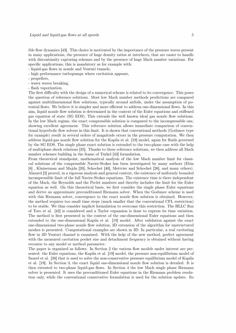
Comparison with the compressible exact solution under low Mach conditions Thefigures 3, 4 and 5 show the low Mach number compressible exact solution versus the incom-pressible exact one. The fluid used corresponds to liquid water while the imposed mass flowrate, m, is equal to 7000Kg.m−2.s−1 and the imposed stagnation enthalpy H is computed us-ing P = 1.0Bar and ρ = 1000Kg.m−3. The geometrical data are those given in Section 3.1.4.The two first graphs show perfect agreement between compressible and incompressible pressureand velocity fields as the flow maximum Mach number is 0.01 . The density profile show slightdeviations. The incompressible solution is obviously constant while the compressible one showsvariations of about 10−5ρ0.
We can thus conclude that in the low Mach regime both exact solutions are in close agreement.The exact single phase nozzle flow solution being now in hand, it is interesting to check theaccuracy of existing numerical methods against these reference solutions.
3.1.7 Behavior of conventional Godunov type schemes in low Mach number condi-tions
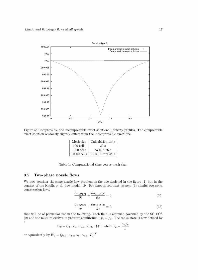
The Godunov scheme for the Euler equations in ducts of smooth varying cross section is consid-ered for the computation of steady liquid nozzle flows. This scheme, with HLLC approximateRiemann solver, is summarized in the Appendix 6 . Computed results are compared with theexact nozzle solution under low Mach number flow conditions, for various meshes of increasingrefinement : 100, 1000 and 10,000 cells. The corresponding results are shown in the Figures 6, 7and 8, again with the same geometrical nozzle parameters as those of the preceding subsection.
The computed and exact velocity profiles are in perfect agreement. This is not the case ofthe pressure field that shows 500% error, due to density fluctuations combined with the SG EOS(2) stiffness. Under mesh refinement the error decreases and quasi convergence is reached with10,000 cells. Table 1 shows computational time to reach steady state versus mesh size. It is clearthat the method is extremely expensive, even for 1D computations.

16 S. LeMartelot, B. Nkonga and R. Saurel
-20000
0
20000
40000
60000
80000
100000
120000
0 0.2 0.4 0.6 0.8 1
x(m)
Pressure (Pa)
Incompressible exact solutionCompressible exact solution
Figure 3: Compressible and incompressible exact solutions : pressure profiles. The two solutionsare merged.
7
8
9
10
11
12
13
14
15
16
17
0 0.2 0.4 0.6 0.8 1
x(m)
Velocity(m/s)
Incompressible exact solutionCompressible exact solution
Figure 4: Compressible and incompressible exact solutions : velocity profiles. The two solutionsare merged.
Liquid and liquid-gas flows at all speeds 17
999.96
999.965
999.97
999.975
999.98
999.985
999.99
999.995
1000
1000
1000.01
0 0.2 0.4 0.6 0.8 1
x(m)
Density (kg/m3)
Incompressible exact solutionCompressible exact solution
Figure 5: Compressible and incompressible exact solutions : density profiles. The compressibleexact solution obviously slightly differs from the incompressible exact one.
Mesh size Calculation time100 cells 20 s1000 cells 33 min 56 s10000 cells 59 h 16 min 48 s
Table 1: Computational time versus mesh size.
3.2 Two-phase nozzle flows
We now consider the same nozzle flow problem as the one depicted in the figure (1) but in thecontext of the Kapila et al. flow model [19]. For smooth solutions, system (3) admits two extraconservation laws,
∂α1ρ1s1
∂t+
∂α1ρ1s1u
∂x= 0, (35)
∂α2ρ2s2
∂t+
∂α2ρ2s2u
∂x= 0, (36)
that will be of particular use in the following. Each fluid is assumed governed by the SG EOS(2) and the mixture evolves in pressure equilibrium : p1 = p2. The tanks state is now defined by:
W0 = (ρ0, u0, α1,0, Y1,0, P0)T , where Yk =
αkρk
ρ
or equivalently by W0 = (ρ1,0, ρ2,0, u0, α1,0, P0)T

18 S. LeMartelot, B. Nkonga and R. Saurel
7
8
9
10
11
12
13
14
15
16
17
0 0.2 0.4 0.6 0.8 1
x(m)
Velocity(m/s)
Godunov scheme + HLLC 100 cellsGodunov scheme + HLLC 1000 cells
Godunov scheme + HLLC 10000 cellsCompressible exact solution
Figure 6: Computed velocity profiles with 100, 1000 and 10,000 cells against the compressibleexact solution. The four solutions are merged.
3.2.1 Critical pressure ratios
The various flow regimes occurring in the Laval nozzle are related, as previously for single phaseflows, to the outlet/inlet pressure ratio.
Critical pressure ratio 1 (cpr1) In this flow regime, the throath has a sonic state, whileit is subsonic elsewhere. To determine the throath pressure associated to the sonic state, thefollowing relations are used:
H∗ = H0, (37)
s1,∗ = s1,0, (38)
s2,∗ = s2,0, (39)
Y1,∗ = Y1,0, (40)
Y2,∗ = Y2,0, (41)
u∗ = c∗. (42)

Liquid and liquid-gas flows at all speeds 19
-200000
-100000
0
100000
200000
300000
400000
500000
0 0.2 0.4 0.6 0.8 1
x(m)
Pressure (Pa)
ExactWithout Mref
Mref = 0.1Local Mref
Figure 7: Computed pressure profiles in the Laval nozzle with 100, 1000 and 10,000 cells againstthe compressible exact solution. The Godunov scheme with coarse mesh predicts a solutionwith a factor 5 error. This error decreases under mesh refinement. Quasi-converged results areobtained for the 10,000 cells mesh.
The total enthalpy is defined by : H = Y1h1+Y2h2+1
2u2. These various relations are expressed
as functions of the pressure :
Y1,0h1,∗(P∗) + Y2,0h2,∗(P∗) +1
2c2∗(P∗) = h0 (43)
with hk,∗ =γk(P∗ + P∞,k)
(γk − 1)ρk,∗.
The isentropes are expressed as :
ρk,∗ = ρk,∗(P∗) = ρk,0
(
P∗ + P∞,k
P0 + P∞,k
)
1
γk (44)
The sound speed of System (3) corresponds to the Wood [45] one :
1
ρ∗c2∗=
α1,∗
ρ1,∗c21,∗
+α2,∗
ρ2,∗c22,∗
(45)
In this relation, the mixture density is determined by :
1
ρ∗=
Y1,0
ρ1,∗(P∗)+
Y2,0
ρ2,∗(P∗)(46)
20 S. LeMartelot, B. Nkonga and R. Saurel
999.9
1000
1000.1
1000.2
1000.3
1000.4
1000.5
1000.6
0 0.2 0.4 0.6 0.8 1
x(m)
Density (kg/m3)
Godunov scheme + HLLC 100 cellsGodunov scheme + HLLC 1000 cells
Godunov scheme + HLLC 10000 cellsCompressible exact solution
Figure 8: Computed density profiles in the Laval nozzle with 100, 1000 and 10,000 cells againstthe compressible exact solution. The Godunov scheme solutions present some fluctuations. Theerror decreases under mesh refinement.
The squared sound speeds are given by their definition :
c2k,∗ = γkP∗ + P∞,k
ρk,∗(P∗)(47)
The volume fractions αk,∗ are determined from the mass fractions definition :
αk,∗ =Yk,0ρ∗(P∗)
ρk,∗ (P∗)(48)
All these relations are used in Relation (43) that forms a non-linear function of P∗. Is is solvedby the Newton-Raphson method. Once the star pressure is determined, all subsequent variablesat the sonic throath are determined.
There is thus no difficulty to determine the first critical pressure ratio (cpr1). To do so, the massflow rate is expressed at throath,
m∗ = ρ∗u∗A∗ (49)
This mass flow rate is the same in the outlet section. Thus, the velocity in the outlet sectionreads,
Uout(Pout) =m∗vout(Pout)
Aout
(50)

Liquid and liquid-gas flows at all speeds 21
where the outlet pressure Pout has to be determined. The specific volumes at the outlet sectionare given by :
vk,out = vk,0
(
P0 + P∞,k
Pout + P∞,k
)
1
γk (51)
and the mixture specific volume reads,
vout = Y1,0v1,out(Pout) + Y2,0v2,out(Pout). (52)
These relations are inserted in the total enthalpy conservation expressed between the tank andthe outlet section :
Y1,0h1,out(Pout) + Y2,0h2,out(Pout) +1
2u2out(Pout)− h0 = 0 (53)
This equation admits two roots. To determine the critical pressure ratio cpr1, the Newton methodis initialized with Pout = P∗. Once Pout is determined, the critical pressure ratio is deduced as:
cpr1 =Pout
P0=
Pcpr1
P0(54)
Critical pressure ratio 3 (cpr3) The same relation (53) is solved with the Newton methodtaking Pout = (1 + 10−6)Min(P∞,1, P∞,2) as initial guess for the outlet pressure.Once Pout isdetermined, the critical pressure ratio is deduced as :
cpr3 =Pout
P0=
Pcpr3
P0(55)
Critical pressure ratio 2 (cpr2) This pressure ratio is associated to the pressure correspond-ing to a steady shock wave in the outlet section. Thus, the flow enters the shock at a pressureequal to Pcpr3. The shock jump relations [36] are used:
(ρu)cpr3 = (ρu)cpr2 (56)
(
ρu2 + P)
cpr3=(
ρu2 + P)
cpr2(57)
e1,cpr2 − e1,cpr3 +Pcpr2 + Pcpr3
2(v1,cpr2 − v1,cpr3) = 0 (58)
e2,cpr2 − e2,cpr3 +Pcpr2 + Pcpr3
2(v2,cpr2 − v2,cpr3) = 0 (59)
Inserting the SG EOS in these two last relations, the specific volumes are expressed as functionsof the shock state pressure :
v1,cpr2
v1,cpr3=
(γ1 − 1)(Pcpr2 + P∞,1) + (γ1 + 1)(Pcpr3 + P∞,1)
(γ1 − 1)(Pcpr3 + P∞,1) + (γ1 + 1)(Pcpr2 + P∞,1)(60)
v2,cpr2
v2,cpr3=
(γ2 − 1)(Pcpr2 + P∞,2) + (γ2 + 1)(Pcpr3 + P∞,2)
(γ2 − 1)(Pcpr3 + P∞,2) + (γ2 + 1)(Pcpr2 + P∞,2)(61)

22 S. LeMartelot, B. Nkonga and R. Saurel
Combining Relations (56) and (57), the following relation is obtained,
Pcpr2 = Pcpr3 + ρcpr3 + ρcpr3u2cpr3
(
1− vcpr2
vcpr3
)
. (62)
The mixture specific volume vcpr2 can be expressed as a function of the pressure Pcrp2 as :
vcrp2 = Y1,0v1,crp2(Pcrp2) + Y2,0v2,crp2(Pcrp2) (63)
Combining these two last relations, a non-linear function of Pcrp2 is obtained.It is solved by the Newton-Raphson method by taking Pcrp2 = Pcrp1 as initial guess. The criticalpressure ratio cpr2 is then deduced as :
cpr2 =Pout
P0(64)
3.2.2 Derivation of the Nozzle flow profile : two-phase isentropic
As for the single phase case, the flow is isentropic when the pressure ratio PR =Pout
P0is either
greater than cpr1 or lower than crp2. The outlet pressure Pout is imposed by the boundaryconditions and the remaining state variables can be determined from :
ρ1,out = ρ1,0
(
Pout + P∞,1
P0 + P∞,1
)
1
γ1 (65)
ρ2,out = ρ2,0
(
Pout + P∞,2
P0 + P∞,2
)
1
γ2 (66)
vout = Y1,0v1,out + Y2,0v2,out (67)
h1,out =γ1 (Pout + P∞,1)
(γ1 − 1) ρ1,out(68)
h2,out =γ1 (Pout + P∞,2)
(γ2 − 1) ρ2,out(69)
αk,out =Yk,0ρout(Pout)
ρk,out(Pout)(70)
The velocity at the outlet is determined from the total enthalpy definition :
Uout =√
2 [h0 − (Y1,0h2,out(Pout) + Y2,0h2,out(Pout))] (71)
From the outlet state knowledge, there is no difficulty to determine the mixture mass flow rate:
m = ρoutUoutAout (72)
In a given area of cross section Ai, the velocity reads:
ui =mvi(Pi)
Ai
, (73)

Liquid and liquid-gas flows at all speeds 23
where the pressure Pi has to be determined. The total enthalpy conservation expressed betweenthe tank and the Ai section reads,
Y1,0h1,i(Pi) + Y2,0h2,i(Pi) +1
2u2(Pi)− h0 = 0 (74)
where the enthalpies h1,i and h2,i are deduced from the same set of relations (65 - 69). Relation(74) is solved by the Newton-Raphson method with Pi = P0 as the initial guess in the nozzleconvergent and Pi = Pout in the nozzle divergent. Once the pressure Pi is determined, the volumefractions are determined by the same relations (70).
3.2.3 Derivation of the Nozzle flow profile : two-phase Adiabatic
When the pressure ratio, PR =Pout
P0is lower than crp1 and greater than crp2 a steady shock wave
appears in the divergent. To determine the shock position we use the same method as previously,for single phase nozzle flows, except that the Rankine-Hugoniot jump relations correspond nowto System (56-59).
3.2.4 Solution examples
The exact solutions calculation is addressed with the same geometry as previously (cf Section3.1.4). The fluids used in the calculations corresponds to liquid water and air, with the followingSG EOS (2) parameters γwater = 4.4, P∞,water = 600MPa, γair = 1.4, P∞,air = 0Pa. The tankstate is defined by :
W0 =
ρ1,0 = 1000Kg.m−3
ρ2,0 = 1Kg.m−3
u0 = 0m.s−1
α1,0 = 0.99999P0 = 1MPa
.
Where subscripts "1" and "2" correspond to the water and the air, respectively. Figure (9) shows
different typical solutions according by their respective pressure ratio PR =Pout
P0. In this case,
critical pressure ratios are respectively :cpr1= 0.80973973,cpr2= 0.40989492,cpr3= 6.9815930.10−8.The pressure profiles corresponding to each pressure ratio are shown in the Figure 9. In addition,an isentropic pressure profile is shown in dashed lines for a subsonic flow in both convergent anddivergent nozzle parts. It corresponds to the pressure ration PR = 0.9. An extra solution exampleis shown with a steady shock in the nozzle divergent. It corresponds to the pressure ratio PR= 0.5. Furthermore, Mach number and water volume fraction profiles are shown in the Figures10, 11 and 12. The sonic state at throath appears for weak pressure ratios (cpr ≤ 0.8) which arequite easy to reach in practical systems. From that pressure ratio, when the outlet pressure islowered (or the tank pressure is increased) part of the divergent is supersonic. The Mach numberincreases dramatically, as the sound speed is non monotonic versus volume fraction. Thus, thegas volume fraction increases as the pressure decreases and cavitation zones appear. It isworth to mention that the the obtained cavitating nozzle flow is "ideal" or "academic", at leastfor two reasons:
1) The cavitation zone that appears in the divergent is not due to liquid-gaz phase changebut only to bubbles growth, imposed by the pressure equilibrium condition.

24 S. LeMartelot, B. Nkonga and R. Saurel
1e-08
1e-07
1e-06
1e-05
0.0001
0.001
0.01
0.1
1
0 0.2 0.4 0.6 0.8 1
P/P
0
x(m)
Pressure Ratio
CPR1CPR2CPR3
Isentropic FlowAdiabatic Flow
Figure 9: Dimensionless pressure profiles in the Laval nozzle for different exit pressures corre-sponding to subsonic flow with sonic throat (cpr1), supersonic isentropic flow (cpr3), flow with asteady shock in the exit section (cpr2), subsonic isentropic solution (PR = 0.9) and steady shockin the divergent (PR = 0.5).
0.001
0.01
0.1
1
10
100
1000
10000
0 0.2 0.4 0.6 0.8 1
Mach n
um
ber
x(m)
Mach number
CPR1CPR2CPR3
Isentropic FlowAdiabatic Flow
Figure 10: Mach number profiles in the Laval nozzle for different exit pressures correspondingto subsonic flow with sonic throat (cpr1), supersonic isentropic flow (cpr3), flow with a steadyshock in the exit section (cpr2), subsonic isentropic solution (PR = 0.9) and steady shock in thedivergent (PR = 0.5).
2) The reference solution derived previously is 1D whereas experimental ones always dealwith multi-D effects. Indeed, cavitation zones correspond to multi-D pockets, separating a

Liquid and liquid-gas flows at all speeds 25
0.9988
0.999
0.9992
0.9994
0.9996
0.9998
1
0 0.2 0.4 0.6 0.8 1
Wate
r volu
me fra
ction
x(m)
Water volume fraction
CPR1Isentropic Flow
Figure 11: Water volume fraction profiles in the Laval nozzle for different exit pressures cor-responding to subsonic flow with sonic throat (cpr1) and subsonic isentropic solution (PR =0.9).
0.4
0.5
0.6
0.7
0.8
0.9
1
0 0.2 0.4 0.6 0.8 1
Wate
r volu
me fra
ction
x(m)
Water volume fraction
CPR2CPR3
Adiabatic Flow
Figure 12: Volume fraction of water profiles in the Laval nozzle for different exit pressurescorresponding to supersonic isentropic flow (cpr3), flow with a steady shock in the exit section(cpr2) and steady shock in the divergent (PR = 0.5).

26 S. LeMartelot, B. Nkonga and R. Saurel
nearly pure gas and a nearly pure liquid in the nozzle.
These multi-D effects also imply velocity disequilibrium in a given cross-section. The two-phasereference solution derived previously is however clearly helpful to examine the accuracy andconvergence of numerical schemes of two-phase nozzle flows computations.
3.2.5 Exact two-phase nozzle solution with imposed mass flow rate and stagnationenthalpy
In many practical situations the inlet is not connected to a tank but has imposed mass inflowand stagnation enthalpy. In other words, the mass flux m0 is imposed as well as the stagnationenthalpy H0, corresponding to imposed total energy flux. For two-phase flows, the mixtureenthalpy reads:
H0 = Y0,1h0,1 + Y0,2h0,2 +1
2u20 (75)
It means that the mass fractions have to be imposed, as well as the volume fraction of one of thephase, α0,1, for example. It is thus necessary to impose m0, hk,0, Yk,0. Another option being toimpose m0, P0, ρk,0 and α1,0. The exact solution determination with such boundary conditionsfollows the same methodology as the one detailed previously with imposed tank conditions. Wedetail hereafter the subsonic isentropic solution only as it is the most important for the presentstudy, that focuses on low Mach number flows.
Outlet state determination The outlet pressure is prescribed as previously and denoted byPout. Using the SG EOS (2) the phase total enthalpy is expressed as follows:
hk =γk(P + P∞,k)vk
(γk − 1)+
1
2u2 (76)
Thus, using the phase total enthalpy conservation between the inlet and the outlet (as we focusonly on the subsonic isentropic solution), we obtain:
hk,0 =γk(Pout + P∞,k)vk,out
(γk − 1)+
1
2u2out (77)
With the help of the mass flow rate conservation (m0 = ρoutAoutUout) and the mixture density
definition (1
ρout= Y1,0v1,out + Y2,0v2,out), the two following equations are obtained:
h1,0 =γ1(Pout + P∞,1)v1,out
(γ1 − 1)+
1
2
(
m0
Aout
)2
(Y1,0v1,out + Y2,0v2,out)2 (78)
h2,0 =γ2(Pout + P∞,2)v2,out
(γ2 − 1)+
1
2
(
m0
Aout
)2
(Y1,0v1,out + Y2,0v2,out)2 (79)
Combining these two relations, we obtain a expression linking v1,out and v2,out:
v1,out =(γ1 − 1)
γ1(Pout + P∞,1)
[
h1,0 − h2,0 +γ2(Pout + P∞,2)v2,out
(γ2 − 1)
]
(80)
Using this expression in Relation (79) a second order polynomial in v2,out is obtained. Keepingthe positive solution, v1,out is obtained using (80). Once v1,out and v2,out are known, the mixturedensity at the outlet section is obtained by,
1
ρout= Y1,0v1,out + Y2,0v2,out (81)

Liquid and liquid-gas flows at all speeds 27
and the outlet velocity is deduced by,
Uout =m0
ρoutAo
. (82)
Last, the volume fractions are determined with the help of mass fractions conservation,
αk,0 = Yk,0ρoutvk,out. (83)
Variables state determination in an arbitrary area As the flow is isentropic between asection of arbitrary area (A) and the outlet section, the phase density can be expressed usingrelations (65 - 66) between the outlet and a section of arbitrary area. Thus, writing the phasetotal enthalpy conservation between a section of arbitrary area and the outlet gives the followingrelation:
hk,out =γk(P + P∞,k)vk(P )
(γk − 1)+
1
2
(m0
A
)2
(Y1,0v1,out(P ) + Y2,0v2,out(P ))2 (84)
The mixture pressure, P , is therefore determined by solving one of these relations using theNewton-Raphson method. Once P is known, the phase densities are determined using (65 - 66)while the other variables are computed as previously.
4 Improving numerical convergence in the low Mach num-
ber limit
We now address the numerical approximation of flow models (1) and (3) corresponding to singlefluid and two-phase fluid respectively. For the sake of simplicity, the analysis is carried out in1D, multi-D extension being addressed later.
4.1 Low Mach number preconditioning
As shown previously, the conventional Godunov method converges to the exact low Mach numbersolution if very fine resolution is used. Such meshes being impracticable for multi-dimensionalapplications, modifications have to be done. We are seeking a numerical method valid for allspeeds flows, from transonic to low Mach number. Transonic and high Mach number conditionsrequire conservative formulation of the equations and corresponding numerical scheme. In thisarea, Riemann problem based methods are recommended. The difficulty with conservative for-mulations is to reach the incompressible limit when the Mach number tends to zero as it is wellknown that corresponding solvers fail to provide an accurate approximation of the incompressibleequations. It seems that the acoustic dissipation process is not efficient enough for finite volumesapproximations using Riemann solvers. Indeed, Riemann solvers are based on acoustic lineariza-tion, which aims to slowly dissipate acoustic waves. Therefore, Riemann solvers preconditioningis needed to manage the numerical dissipation in order to improve the numerical convergence atlow Mach number limit. In order to achieve this goal, Turkel [43] proposed to enforce pressuretime invariance up to Mach number square fluctuations with the help of a penalization method.In the context of Riemann solvers, this penalization can be applied to modify the Riemann prob-lem solution while the conservative formulation and real equation of state are still used during thesolution update. This strategy is presented hereafter in the context of the Euler equations first,the multiphase flow formulation being addressed latter. The HLLC Riemann solver of Toro et al.[42] is considered and wave’s speeds for all Mach number flow situations are estimated following

28 S. LeMartelot, B. Nkonga and R. Saurel
Braconnier and Nkonga [6] with the help of the following analysis. For the approximate Riemannproblem resolution, the Euler equations are considered under primitive variables formulation:
∂ρ
∂t+ ρ
∂u
∂x+ u
∂ρ
∂x= 0
∂u
∂t+ u
∂u
∂x+
1
ρ
∂p
∂x= 0
∂p
∂t+ u
∂p
∂x+ ρc2
∂u
∂x= 0
(85)
4.1.1 Dimensionless variables
These equations are expressed in dimensionless variables with the help of the following definitions: ρ = [ρ]ρ, u = [u]u, p = [p]p, x = [x]x and t = [t]t, where [f ] represents a characteristic scale ofthe corresponding variable and f the dimensionless one. System (85) becomes :
∂ρ
∂t+ ρ
∂u
∂x+ u
∂ρ
∂x= 0
∂u
∂t+ u
∂u
∂x+
[p]
[ρ][u]2ρ
∂p
∂x= 0
∂p
∂t+ u
∂p
∂x+
[ρ][c]2
[p]ρc2
∂u
∂x= 0
(86)
A pressure scaling has to defined. At least, two options are possible:- An ’acoustic’ scaling, corresponding to,
[p] = [ρ][c][u] (87)
- A ’bulk modulus’ scaling, corresponding to,
[p] = [ρ][c]2 (88)
These different pressure scales result in two dimensionless Euler equations. The existence ofthese two branches is precisely at the basis of conventional algorithms convergence difficulties.As illustrated in the Figures (7 - 8) the Godunov scheme has low dissipation of the acousticsscale and consequently presents convergence issues. As shown in the next subsection, the ’bulkmodulus scaling’,
∂ρ
∂t+ ρ
∂u
∂x+ u
∂ρ
∂x= 0
∂u
∂t+ u
∂u
∂x+
1
M2ρ
∂p
∂x= 0
∂p
∂t+ u
∂p
∂x+ ρc2
∂u
∂x= 0,
(89)
formally admits the incompressible Euler equations as asymptotic limit when the Mach numbertends to zero. We thus consider System (89) in the following where the symbol ∼ is dropped forthe sake of simplicity.
4.1.2 Asymptotic analysis
We now examine the limit system associated to System (89) when the Mach number tends tozero. To do so, an asymptotic analysis is done. The various flow variables ’f’ are expanded as:
f = f0 + ǫf1 + ǫ2f2, where ǫ → 0+.

Liquid and liquid-gas flows at all speeds 29
A the order ǫ−2 System (89) implies,∂p0
∂x= 0 (90)
A the order ǫ−1 it implies,∂p1
∂x= 0 (91)
and at leading order the limit system reads:
∂ρ0
∂t+ u0
∂ρ0
∂x+ ρ0
∂u0
∂x= 0
∂u0
∂t+ u0
∂u0
∂x+
1
ρ0
∂p2
∂x= 0.
∂p0
∂t+ ρ0c
20
∂u0
∂x= 0
(92)
Under the condition,∂p0
∂t= 0, (93)
System (92) tends formally to the incompressible Euler equations when the Mach number tendsto zero. Indeed, the incompressible Euler equations read:
ρ0 = const.
∂u0
∂x= 0
∂u0
∂t+ u0
∂u0
∂x+
1
ρ0
∂p2
∂x= 0
(94)
To enforce condition (93), an extra coefficient is added to the pressure equation of System (92):
1
M2
∂p0
∂t+ ρ0c
20
∂u0
∂x= 0 (95)
This penalization strategy, due to Turkel [43], forces solutions of System (92) to converge toincompressible solutions.
4.1.3 System considered for the Riemann problem
Inserting (95) in (92) and using (90 - 91), the following leading order system is obtained:
∂ρ
∂t+ u
∂ρ
∂x+ ρ
∂u
∂x= 0
∂u
∂t+ u
∂u
∂x+
1
ρ
∂p
∂x= 0.
∂p
∂t+M2u
∂p
∂x+M2ρc2
∂u
∂x= 0
(96)
This system is hyperbolic and has the following wave speeds: u, u+ c+, u− c−, with,
c− =(1−M2)u+
√
(M2 − 1)2u2 + 4M2c2
2(97)
30 S. LeMartelot, B. Nkonga and R. Saurel
c+ =(M2 − 1)u+
√
(M2 − 1)2u2 + 4M2c2
2(98)
These wave speeds are directly used in the HLLC solver (136).It is worth to mention that the Euler system is modified in the Riemann problem resolution only,where formulation (96) is used. With the fluxes computed with the HLLC solver, the Godunovmethod (135) is used with the conventional conservative formulation of the Euler equations andunmodified equation of state.Thus, the flow model solved corresponds exactly to System (1) with the EOS (2). This methodobviously guarantees conservation and correct jumps across waves. It only acts on the numericaldissipation.As the conservative formulation is used, even strong discontinuities can be handled by themethod. Also, as the Mach number can be chosen in (96), the method is able to computefast flows. This remarkable feature has been observed and analyzed by Guillard and Viozat[12]. The validity and efficiency of this method is illustrated in Section 4 where comparisonswith the exact solution are done, showing excellent agreement even when coarse meshes are usedcompared to the original Godunov method. We now address method extension to the two-phaseflow model (3) and its pressure non equilibrium variant (5).
4.1.4 Two-phase low Mach preconditioning
The pressure non-equilibrium model (5) in primitive form reads:
∂α1
∂t+ u
∂α1
∂x= 0
∂α1ρ1
∂t+ α1ρ1
∂u
∂x+ u
∂α1ρ1
∂x= 0
∂α2ρ2
∂t+ α2ρ2
∂u
∂x+ u
∂α2ρ2
∂x= 0
∂u
∂t+ u
∂u
∂x+
1
ρ
∂P
∂x= 0
∂e1
∂t+ u
∂e1
∂x+
p1
ρ1
∂u
∂x= 0
∂e2
∂t+ u
∂e2
∂x+
p2
ρ2
∂u
∂x= 0
∂P
∂t+ u
∂P
∂x+ ρc2
∂u
∂x= 0
(99)
The pressure relaxation terms have been omitted as they are solved separately. This systemadmits the following frozen sound speed defined by:
cf =√
Y1c21 + Y2c
22 (100)
This sound speed is very different from the mechanical equilibrium one given by (45). However,the equilibrium sound speed is recovered after the projection to pressure equilibrium summarizedin Section 2.As System (5) is overdetermined (see again Section 2 for details), its primitive variables formu-lation is also overdetermined. In particular, the mixture pressure equation and the two internal

Liquid and liquid-gas flows at all speeds 31
energy equations form an overdetermined subsystem.During low Mach preconditioning, in order to force the incompressibility condition,
∂u
∂x= 0, (101)
when the Mach number tends to zero, the pressure equation has been modified with a penalizationcoefficient (Equation 95), resulting in System (96) in the single phase flows context. Here, thesame preconditioned pressure formulation is adopted:
1
M2
∂P
∂t+ u
∂P
∂x+ ρc2
∂u
∂x= 0 (102)
Modifying the mixture pressure equation (P = α1p1 + α2p2) that appears in the momentumequation immediately modifies the wave speeds, as previously in the single phase flow case:
c− =(1−M2)u+
√
(M2 − 1)2u2 + 4M2c2f
2(103)
c+ =(M2 − 1)u+
√
(M2 − 1)2u2 + 4M2c2f
2(104)
Note that the Mach number that appears in the equations (103 - 104) is defined with the samesound speed (100). It means that, in the low Mach number limit, the following system is solved:
∂α1
∂t+ u
∂α1
∂x= 0,
∂ρ1
∂t+ u
∂ρ1
∂x= 0,
∂ρ2
∂t+ u
∂ρ2
∂x= 0,
∂u
∂t+ u
∂u
∂x+
1
ρ
∂P
∂x= 0,
∂p1
∂t+ u
∂p1
∂x= 0 or alternatively
∂e1
∂t+ u
∂e1
∂x= 0,
∂p2
∂t+ u
∂p2
∂x= 0 or alternatively
∂e2
∂t+ u
∂e2
∂x= 0,
∂u
∂x= 0
(105)
Knowledge of the limit internal energy equations will be of particular help for the low MachRiemann solver presented hereafter.
Solving the Riemann problem Using the following notations :
Sl = ul − cl = ul −(1−M2)ul +
√
(M2 − 1)2u2l + 4M2c2l
2(106)
Sr = ur + cr = ur +(M2 − 1)ur +
√
(M2 − 1)2u2r + 4M2c2r
2(107)

32 S. LeMartelot, B. Nkonga and R. Saurel
And with HLL SM approximation :
SM =SR(ρu)R − SL(ρu)L − ((ρu2 + p)R − (ρu2 + p)L)
SRρR − SLρL − ((ρu)R − (ρu)L)(108)
The corresponding Riemann problem can be represented as :
Figure 13: Description of the Riemann problem and associated wave speeds.
The Riemann problem is solved as explained in [38], except for the internal energy equations.The variables vector, U , and the flux vector, F , are defined as follows:
U =
α1
α1ρ1α2ρ2α1ρ1e1α2ρ2e2ρu
ρE
F =
α1u
α1ρ1u
α2ρ2u
α1ρ1e1u
α2ρ2e2u
ρu2 + P
(ρE + P )u
(109)
Using the low Mach number preconditioning leads to∂u
∂x= 0, which means that the internal
energy equations can be re-written as:
∂e1
∂t+ u
∂e1
∂x= 0
∂e2
∂t+ u
∂e2
∂x= 0
(110)
Therefore, there is no internal energy jump through the Sl and Sr waves.Thus, the only modifications to the Riemann problem solving are the following:
e∗k,L = ek,L
e∗k,R = ek,R(111)
4.2 Preconditionned Riemann solvers illustrations
4.2.1 Single phase nozzle flow
The explicit Godunov scheme of Appendix 6 with HLLC Riemann solver is used, with the pre-conditioned wave speed (97 - 98 ) derived previously. The single phase Euler equations are firstconsidered.
In the formulation (96), and consequently in the associated Riemann solver, given in Appendix

Liquid and liquid-gas flows at all speeds 33
6, the Mach number M is set to a reference value Mref which is used as constant in the entireflow field or variable at each cell boundary. To illustrate the method efficiency the same nozzleflow problem as studied previously in Figures (6 - 8) is considered.A coarse mesh with 100 grid points is considered and the Mref influence is studied. Correspond-ing results are shown in the Figures (14 - 15) at steady state.
-200000
-100000
0
100000
200000
300000
400000
500000
0 0.2 0.4 0.6 0.8 1
x(m)
Pressure (Pa)
ExactWithout Mref
Mref = 0.1Local Mref
Figure 14: Computed pressure profiles in the Laval nozzle test with Mref=0.1, Mref=localMach number and without Mref are compared against the compressible exact solution. Theerror decreases dramatically as soon as Mref is used and tends to the local Mach number.
4.2.2 Two phase nozzle flow
To illustrate the two-phase low Mach number preconditioning, the same nozzle flow problem asstudied previously is considered. However, the liquid water at the inflow now contains a smallfraction of air.Mass flow rate and total enthalpy are imposed at left while the right outlet is opened to theatmosphere. The fluids used in the calculations correspond to liquid water and air, with thefollowing SG EOS (2) parameters γwater = 4.4, P∞,water = 600MPa, γair = 1.4, P∞,air = 0Pa.The imposed conditions at left are the following:
m = 6500Kg.m−2.s−1
ρwater = 1000Kg.m−3
ρair = 1Kg.m−3
αwater,0 = 0.9999P = 0.1MPa
The imposed total enthalpy is computed with ρwater, ρair, αwater,0 and P . With these boundaryconditions, the numerical solution has been computed using different values of Mref,min: 0.1,

34 S. LeMartelot, B. Nkonga and R. Saurel
999.9
1000
1000.1
1000.2
1000.3
1000.4
1000.5
0 0.2 0.4 0.6 0.8 1
x(m)
Density (Kg/m-3)
ExactWithout Mref
Mref = 0.1Local Mref
Figure 15: Computed density profiles in the Laval nozzle test with Mref=0.1, Mref=local Machnumber and without Mref are compared against the compressible exact solution. The errordecreases dramatically as soon as Mref is used and tends to the local Mach number.
0.05, 0.01 and two meshes containing 100 cells and 200 cells, respectively. Mref,min will bedefined in the next subsection.
The following figures show clearly that the waves’ speeds choice and the modification of thesolver has dramatic consequences on method convergence in the low Mach number limit. It isalso clear that the more Mref tends to the true Mach number, in the low Mach limit, the betterthe solution is.
4.2.3 Preconditioning method precautions
It appears clearly that the waves’ speeds choice in the HLLC solver has dramatic consequenceson method convergence in the low Mach number limit. It is also clear that the more Mref tendsto the local Mach number, in the low Mach limit, the better the accuracy is. Therefore, the bestsolution consists in setting the reference Mach number, Mref , to the local one, Mi. But, as the"sound speeds" (97 - 98) tend to wrong values when M tends to 0, the following function is used:
M iref =
1, if Mi ≥ 0.3Mi, if 0.3 > Mi > Mref,min
Mref,min, if Mi ≤ Mref,min
(112)
The minimum Mach number, Mref,min is typically 10−2 or 10−3. The preconditioned soundspeeds must be computed with a unique M∗
ref at a given cell boundary for the Riemann problemresolution:
M∗ref = Max(ML
ref ,MRref ) (113)
Where the superscripts "L" and "R" denote the left and right states of a cell boundary.It is also important to report the computational cost to reach steady state on the previous

Liquid and liquid-gas flows at all speeds 35
6
7
8
9
10
11
12
13
14
15
0 0.2 0.4 0.6 0.8 1
x(m)
Velocity (m/s)
Mref_min=0.1Mref_min=0.05Mref_min=0.01
Mref_min=0.01|200 cellsExact
0
20000
40000
60000
80000
100000
120000
140000
0 0.2 0.4 0.6 0.8 1
x(m)
Pressure (Pa)
Mref_min=0.1Mref_min=0.05Mref_min=0.01
Mref_min=0.01|200 cellsExact
Figure 16: Computed mixture pressure and velocity profiles in the nozzle using different valuesof Mref against the compressible exact solution. The error decreases dramatically as soon asMref is used and tends to the local Mach number.
computational example with this method . It is worth to mention that the stability restriction forsuch scheme is more restrictive than conventional CFL criterion for compressible flows. Indeed,the time step has to fulfill (Birken and Meister, 2005 [5]):
∆t ≤ Mref
∆x
Max(|u|+ c)(114)
This explains the computational costs reported in the Tables (2 - 3):The corresponding Godunov scheme with the low Mach preconditioning is thus accurate but
still expensive due to the time step restriction (114). Is is thus mandatory to derive an implicit

36 S. LeMartelot, B. Nkonga and R. Saurel
986
988
990
992
994
996
998
1000
0 0.2 0.4 0.6 0.8 1
x(m)
Mixture density (Kg.m-3)
Mref_min=0.1Mref_min=0.05Mref_min=0.01
Mref_min=0.01|200 cellsExact
0.986
0.988
0.99
0.992
0.994
0.996
0.998
1
0 0.2 0.4 0.6 0.8 1
x(m)
Water volume fraction
Mref_min=0.1Mref_min=0.05Mref_min=0.01
Mref_min=0.01|200 cellsExact
Figure 17: Computed mixture density and water volume fraction profiles in the nozzle usingdifferent values of Mref against the compressible exact solution. The error decreases dramaticallyas soon as Mref is used and tends to the local Mach number.
Mref,min CPU0.1 3min 17s
Local Mach 1h 23min 12s
Table 2: Computational time versus Mref for the Laval single phase nozzle test problem with100 cells.
scheme.

Liquid and liquid-gas flows at all speeds 37
Mref,min CPU0.1 4min 06s0.01 44min0.01 2h 36min (200 cells)
Table 3: Computational time versus Mref for the Laval two-phase nozzle test problem with100 cells and 200 cells.
4.3 Implicit scheme for the Euler equations
As shown previously, the stability condition associated to preconditioned schemes is decreasedby a factor proportional to the reference Mach number. It turns out that the resulting explicitschemes time steps are dramatically small. In order to overcome stability restrictions, an implicitscheme has to be used. For the sake of simplicity, the implicit scheme is first presented for theEuler equations in 1D. Multi-D and multiphase extensions will be addressed later.
4.3.1 Implicit Godunov scheme
On the basis of the explicit Godunov scheme (135), the implicit version reads:
Un+1i − Un
i = −∆t
∆x(Fn+1
i+ 1
2
− Fn+1i− 1
2
) (115)
Where the flux vectors Fn+1i+ 1
2
and Fn+1i− 1
2
are computed according to variables at time tn+1. Under
Taylor expansion, the flux vectors become:
Fn+1i+ 1
2
= Fni+ 1
2
+∂Fi+ 1
2
∂Ui
)n
(Un+1i − Un
i ) +∂Fi+ 1
2
∂Ui+1
)n
(Un+1i+1 − Un
i+1) (116)
Fn+1i− 1
2
= Fni− 1
2
+∂Fi− 1
2
∂Ui
)n
(Un+1i − Un
i ) +∂Fi− 1
2
∂Ui−1
)n
(Un+1i−1 − Un
i−1) (117)
The flux appearing in these formulas, Fni+ 1
2
, is solution of the Riemann problem and is conse-
quently function of the left and right states: Fni+ 1
2
= F ∗(
Uni , U
ni+1
)
. The Riemann solver used
here is the HLLC solver, already presented (136). Let’s denote the variation:
δUi = Un+1i − Un
i (118)
Rewriting Relations (115), (116) and (117) using (118), the following scheme is obtained:
δUi
[
I +∆t
∆x
∂Fi+ 1
2
∂Ui
)n
− ∆t
∆x
∂Fi− 1
2
∂Ui
)n]
+∆t
∆x
∂Fi+ 1
2
∂Ui+1
)n
δUi+1 −∆t
∆x
∂Fi− 1
2
∂Ui−1
)n
δUi−1 (119)
= −∆t
∆x(Fn
i+ 1
2
− Fni− 1
2
)
Under compact form it reads: MδU = D with
M =
A C (0)B . .
. . .. . .
. . C(0) B A
, δU =
δU1
.
.
.
δUN
, D =
.
.
−∆t
∆x(Fn
i+ 1
2
− Fni− 1
2
)
.
.

38 S. LeMartelot, B. Nkonga and R. Saurel
where the matrixes A, B and C are defined as follows:
A = I3 +∆t
∆x
∂Fi+ 1
2
∂Ui
)n
− ∆t
∆x
∂Fi− 1
2
∂Ui
)n
B = −∆t
∆x
∂Fi− 1
2
∂Ui−1
)n
C =∆t
∆x
∂Fi+ 1
2
∂Ui+1
)n
This tridiagonal system can be solved either by direct or by iterative methods. It is worthto mention that this method is a particular case of the Newton-Raphson method which canbe presented as follows. Let’s consider the function G(δU) whose components are Gi(δU) =
δU +∆t
∆x(Fn+1
i+ 1
2
− Fn+1i− 1
2
). The goal is to solve,
G(δU) = 0. (120)
As Fn+1i+ 1
2
and Fn+1i− 1
2
are non-linear functions of δUi, one way to solve this equation is to use the
Newton-Raphson metho, which, in this case, reads:
G(δUk+1) = G(δUk) +
(
∂G(δUk)
∂δUk
)
(
δUk+1 − δUk)
(121)
As the G(δUk+1) = 0 condition has to be reached, the following formula is obtained:
δUk+1 = δUk −[(
∂G(δUk)
∂δUk
)]−1
G(δUk) (122)
where δUk represents δU at the k step of the iterative method. For practical applications, one ortwo iterations only are used. The present implicit Godunov type scheme needs an approximateRiemann solver to compute the numerical fluxes Fn
i± 1
2
as well as the various flux derivatives.
4.3.2 Flux derivatives
As mentioned before, the HLLC flux (136), as many other Riemann solvers, can be formulatedunder the form:
FLR =1
2(FL + FR)−
1
2
nw∑
j
sign(λj)δWj (123)
Where λj is the speed of the jth wave and δWj is the associated variable jump across thecorresponding wave.With these notations, the fluxes derivatives read:
∂FLR
∂UL
=1
2
∂FL
∂UL
− 1
2
nw∑
j
sign(λj)∂δWj
∂UL
(124)
∂FLR
∂UR
=1
2
∂FR
∂UR
− 1
2
nw∑
j
sign(λj)∂δWj
∂UR
(125)
The calculation details for the HLLC Riemann solver are given in the Appendix 6 .

Liquid and liquid-gas flows at all speeds 39
4.3.3 Illustrations
To illustrate the implicit scheme efficiency, we consider the same test problem as before (Section4.2.1).A coarse mesh with 100 grid points is considered. Corresponding results are shown in theFigures (18 - 19) at steady state. As expected, the implicit scheme is numerically stable for
-20000
0
20000
40000
60000
80000
100000
120000
140000
160000
0 0.2 0.4 0.6 0.8 1
x (m)
Pressure (Pa)
ExplicitImplicit
Exact
Figure 18: Computed pressure profiles in the Laval nozzle with Mref = Mi compared againstthe compressible exact solution. Implicit and explicit solutions show excellent agreement.
999.9
999.95
1000
1000.05
1000.1
0 0.2 0.4 0.6 0.8 1
x (m)
Density (Kg.m-3)
ExplicitImplicit
Exact
Figure 19: Computed density profiles in the Laval nozzle with Mref = Mi compared against thecompressible exact solution. Implicit and explicit solutions show excellent agreement.
larger time steps. It is worth to mention that the computational time is now 4 min, with a CFL

40 S. LeMartelot, B. Nkonga and R. Saurel
coefficient equal to 0.15, to be compared to the computational time of 43 min needed by theexplicit scheme, with a CFL coefficient equal to 0.0036 (As using the low Mach preconditioningwith an explicit scheme requires the use of a time step reduced by a factor Mref,min).
4.4 Multi-D extension
Multidimensional finite volume approximation is addressed. Let’s consider a cell, i, and denoteby V o(i) the set of neighbouring cells as shown in the Figure 20. Therefore, the implicit Godunov
Figure 20: Schematic representation of a triangular cell with its set of neighbours, V o(i) =V1, V2, V3
finite volumes scheme reads:
(Un+1i − Un
i ) = − ∆t
V (i)
∑
j∈V o(i)
Fn+1i,j (126)
Under similar notations as in 1D, the fluxes are expanded as follows:
Fn+1i,j = Fn
i,j +∂Fi,j
∂Ui
)n(
Un+1i − Un
i
)
+∂Fi,j
∂Uj
)n(
Un+1j − Un
j
)
(127)
Denoting the variation by δUi = Un+1i − Un
i and using (127) in (126) the following scheme isobtained:
I +∆t
V (i)
∑
j∈V o(i)
Ajii
δUi +∆t
V (i)
∑
j∈V o(i)
(
AjijδUj
)
= − ∆t
V (i)
∑
j∈V o(i)
Fn+1i,j (128)
with
Ajii =
∂Fi,j
∂Ui
)n
Ajij =
∂Fi,j
∂Uj
)n
Under compact form it reads:MδU = D
where
δU =
δU1
.
.
.
δUN
, D =
.
.
− ∆t
V (i)
∑
j∈V o(i) Fn+1i,j S(ij)
.
.
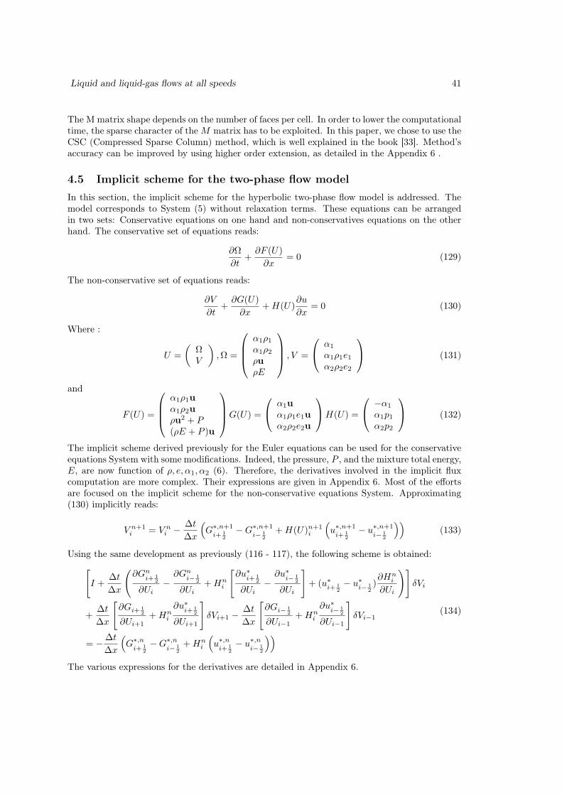
Liquid and liquid-gas flows at all speeds 41
The M matrix shape depends on the number of faces per cell. In order to lower the computationaltime, the sparse character of the M matrix has to be exploited. In this paper, we chose to use theCSC (Compressed Sparse Column) method, which is well explained in the book [33]. Method’saccuracy can be improved by using higher order extension, as detailed in the Appendix 6 .
4.5 Implicit scheme for the two-phase flow model
In this section, the implicit scheme for the hyperbolic two-phase flow model is addressed. Themodel corresponds to System (5) without relaxation terms. These equations can be arrangedin two sets: Conservative equations on one hand and non-conservatives equations on the otherhand. The conservative set of equations reads:
∂Ω
∂t+
∂F (U)
∂x= 0 (129)
The non-conservative set of equations reads:
∂V
∂t+
∂G(U)
∂x+H(U)
∂u
∂x= 0 (130)
Where :
U =
(
ΩV
)
,Ω =
α1ρ1α1ρ2ρuρE
, V =
α1
α1ρ1e1α2ρ2e2
(131)
and
F (U) =
α1ρ1uα1ρ2uρu2 + P
(ρE + P )u
G(U) =
α1uα1ρ1e1uα2ρ2e2u
H(U) =
−α1
α1p1α2p2
(132)
The implicit scheme derived previously for the Euler equations can be used for the conservativeequations System with some modifications. Indeed, the pressure, P , and the mixture total energy,E, are now function of ρ, e, α1, α2 (6). Therefore, the derivatives involved in the implicit fluxcomputation are more complex. Their expressions are given in Appendix 6. Most of the effortsare focused on the implicit scheme for the non-conservative equations System. Approximating(130) implicitly reads:
V n+1i = V n
i − ∆t
∆x
(
G∗,n+1
i+ 1
2
−G∗,n+1
i− 1
2
+H(U)n+1i
(
u∗,n+1
i+ 1
2
− u∗,n+1
i− 1
2
))
(133)
Using the same development as previously (116 - 117), the following scheme is obtained:
[
I +∆t
∆x
(
∂Gni+ 1
2
∂Ui
−∂Gn
i− 1
2
∂Ui
+Hni
[
∂u∗i+ 1
2
∂Ui
−∂u∗
i− 1
2
∂Ui
]
+ (u∗i+ 1
2
− u∗i− 1
2
)∂Hn
i
∂Ui
)]
δVi
+∆t
∆x
[
∂Gi+ 1
2
∂Ui+1+Hn
i
∂u∗i+ 1
2
∂Ui+1
]
δVi+1 −∆t
∆x
[
∂Gi− 1
2
∂Ui−1+Hn
i
∂u∗i− 1
2
∂Ui−1
]
δVi−1
= −∆t
∆x
(
G∗,n
i+ 1
2
−G∗,n
i− 1
2
+Hni
(
u∗,n
i+ 1
2
− u∗,n
i− 1
2
))
(134)
The various expressions for the derivatives are detailed in Appendix 6.
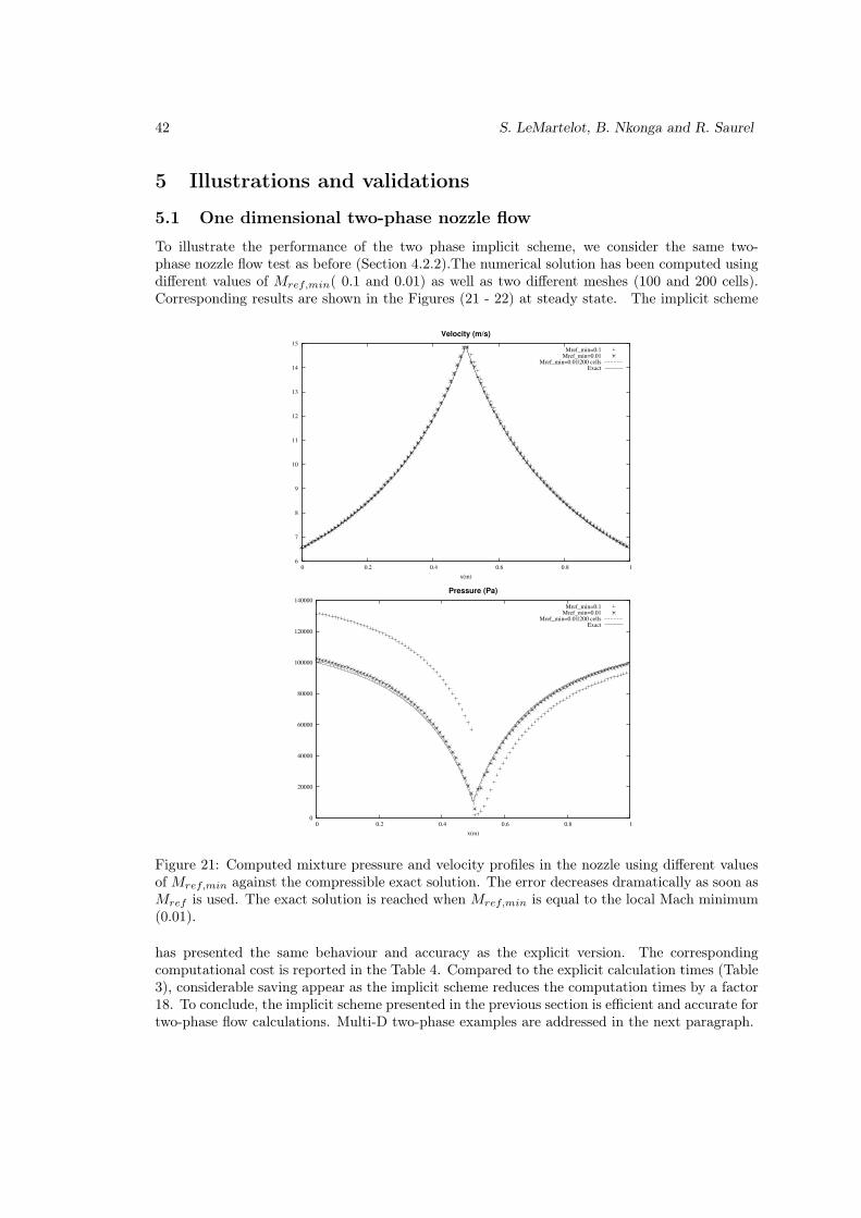
42 S. LeMartelot, B. Nkonga and R. Saurel
5 Illustrations and validations
5.1 One dimensional two-phase nozzle flow
To illustrate the performance of the two phase implicit scheme, we consider the same two-phase nozzle flow test as before (Section 4.2.2).The numerical solution has been computed usingdifferent values of Mref,min( 0.1 and 0.01) as well as two different meshes (100 and 200 cells).Corresponding results are shown in the Figures (21 - 22) at steady state. The implicit scheme
6
7
8
9
10
11
12
13
14
15
0 0.2 0.4 0.6 0.8 1
x(m)
Velocity (m/s)
Mref_min=0.1Mref_min=0.01
Mref_min=0.01|200 cellsExact
0
20000
40000
60000
80000
100000
120000
140000
0 0.2 0.4 0.6 0.8 1
x(m)
Pressure (Pa)
Mref_min=0.1Mref_min=0.01
Mref_min=0.01|200 cellsExact
Figure 21: Computed mixture pressure and velocity profiles in the nozzle using different valuesof Mref,min against the compressible exact solution. The error decreases dramatically as soon asMref is used. The exact solution is reached when Mref,min is equal to the local Mach minimum(0.01).
has presented the same behaviour and accuracy as the explicit version. The correspondingcomputational cost is reported in the Table 4. Compared to the explicit calculation times (Table3), considerable saving appear as the implicit scheme reduces the computation times by a factor18. To conclude, the implicit scheme presented in the previous section is efficient and accurate fortwo-phase flow calculations. Multi-D two-phase examples are addressed in the next paragraph.

Liquid and liquid-gas flows at all speeds 43
986
988
990
992
994
996
998
1000
0 0.2 0.4 0.6 0.8 1
x(m)
Density (Kg.m-3)
Mref_min=0.1Mref_min=0.01
Mref_min=0.01|200 cellsExact
0.986
0.988
0.99
0.992
0.994
0.996
0.998
1
0 0.2 0.4 0.6 0.8 1
x(m)
Volume fraction of water
Mref_min=0.1Mref_min=0.01
Mref_min=0.01|200 cellsExact
Figure 22: Computed mixture pressure and water volume fraction profiles in the nozzle usingdifferent values of Mref,min against the compressible exact solution. The error decreases dra-matically as soon as Mref . The exact solution is reach when Mref,min is equal to the local Machminimum (0.01).
Mref,min CPU Implicit CFL Explicit CFL0.1 46s 3.0 0.090.01 8min 45s (200 cells) 1.5 0.009
Table 4: Computational time versus Mref for the Laval two phase nozzle test problem with theimplicit scheme.

44 S. LeMartelot, B. Nkonga and R. Saurel
5.2 3D Computations of cavitating flows in Venturi channels
In this paragraph, a 3D two phase nozzle flow case is addressed. We first present the geometryand the test parameters. Then, numerical results are compared against the experimental records.
5.2.1 Test case presentation
The experimental facility has been built at LEGI Laboratory, Grenoble, France by the groupleaded by S. Barre. The test section corresponds to a Venturi channel with a nozzle divergentinclined at an angle of 8°. The geometry is shown in the Figure 23: The corresponding point
Figure 23: LEGI 8° Venturi geometry
coordinates are given in the Table 5 : As phase transition occurs at the throat, heat and mass
X (abscissa) (m) Y (m) X(abscissa) (m) Y (m)A 0 0 E 1.225 -0.114B 0.1 0 F 0 0.0488C 0.153 0.0157 G 0.271 0.0488D 0.588 -0.0517 H 1.233 -0.00845
Table 5: Venturi 8° points coordinates.
transfer have to be considered. These effects are accounted for by considering extra relaxationeffects in addition to pressure relaxation. Indeed, as detailed in Saurel et al. [39], temperature andGibbs free energy relaxation have to be considered. Appropriate relaxation solver is summarizedin the appendix 6. Simulating phase transition requires appropriate EOS parameters. The fluidsconsidered correspond to liquid water and water vapor, with the following SG EOS (2) parametersγliq = 1.234, P∞,liq = 2532.302Atm, γvap = 1.316 and P∞,air = 0Pa. These parameters havebeen computed following the method detailed in [27].
Inflow mass flow rate and total enthalpy are imposed and a prescribed pressure is imposedat the outlet. The imposed conditions at the left inflow entrance are the following,
m = 7514.917Kg.m−2.s−1
ρliq = 1067.566Kg.m−3
ρvap = 0.387Kg.m−3
αliq = 0.999P = 51825Pa
while, at the right outlet, the prescribed pressure is P = 72025Pa.

Liquid and liquid-gas flows at all speeds 45
5.2.2 Experimental results
The 8° Venturi channel of Figure 23 has been used at LEGI(Grenoble, France) to create cavitatingglows. With the boundary conditions reported in the previous paragraph, a periodic flow isobserved, as shown in the Fig 24. In the first stage of the cycle (a), a cavitation sheet is attached
Figure 24: Instantaneous pictures of a break off cycle. Courtesy of S.Barre, LEGI, Grenoble,France.
to the throat and grows. In a second stage, the sheet reaches its maximum length (b) and breaksin two parts (c). At the end, the downstream part is swept along within the stream and startsto collapse while the attached part starts another cycle (d). The mean attached cavity lengthvalue is 45 ± 5 mm while the quasi-periodic vapor clouds shedding frequency is about 45 Hz. Itis worth to mention that the cloud shedding frequency was calculated using spectral analysis ofpressure measurement in the Venturi divergent.
5.2.3 Numerical results
A 3D unstructured mesh contain 52450 cells is used (Fig. 25). The grid is refined at the throat inorder to capture the cavitation pocket. The average cell size is 0.013 mm at the throat and 0.08mm elsewhere. As a Venturi geometry is 2D, there is only one cell in the z-direction. Using thismesh with the two-phase 3D implicit scheme along with the two phase low Mach preconditioning(Mref,min is set to 0.04) on a cluster with 24 CPU, allowed to reach 1.8s of physical time in about97h with an average CFL coefficient equals to 28. This physical time was long enough to obtaina quasi-stationary flow with quasi-periodic vapor clouds shedding. An example of the obtainedcloud shedding is shown in the volume fraction contours of Figure 26. A pressure signal is alsorecorded using a numerical jauge located in the middle of the EH segment, at the end of theVenturi divergent (Fig. 23). Using the water vapor volume fraction, we were able to determinea vapor clouds shedding frequency of about 43Hz. In order to verify this observed frequency,a spectral analysis of the recorded pressure signal was performed. The obtained spectrum isshown in the Figure. 27. The maximum intensity is reach for frequencies between 40 and 50Hz,which is in excellent agreement with the observed clouds shedding frequency. By performingmeasurements during every cycle, an average attached cavity length of about 45 mm has beenmeasured from the computations. This results show remarkable agreement with the experiments.
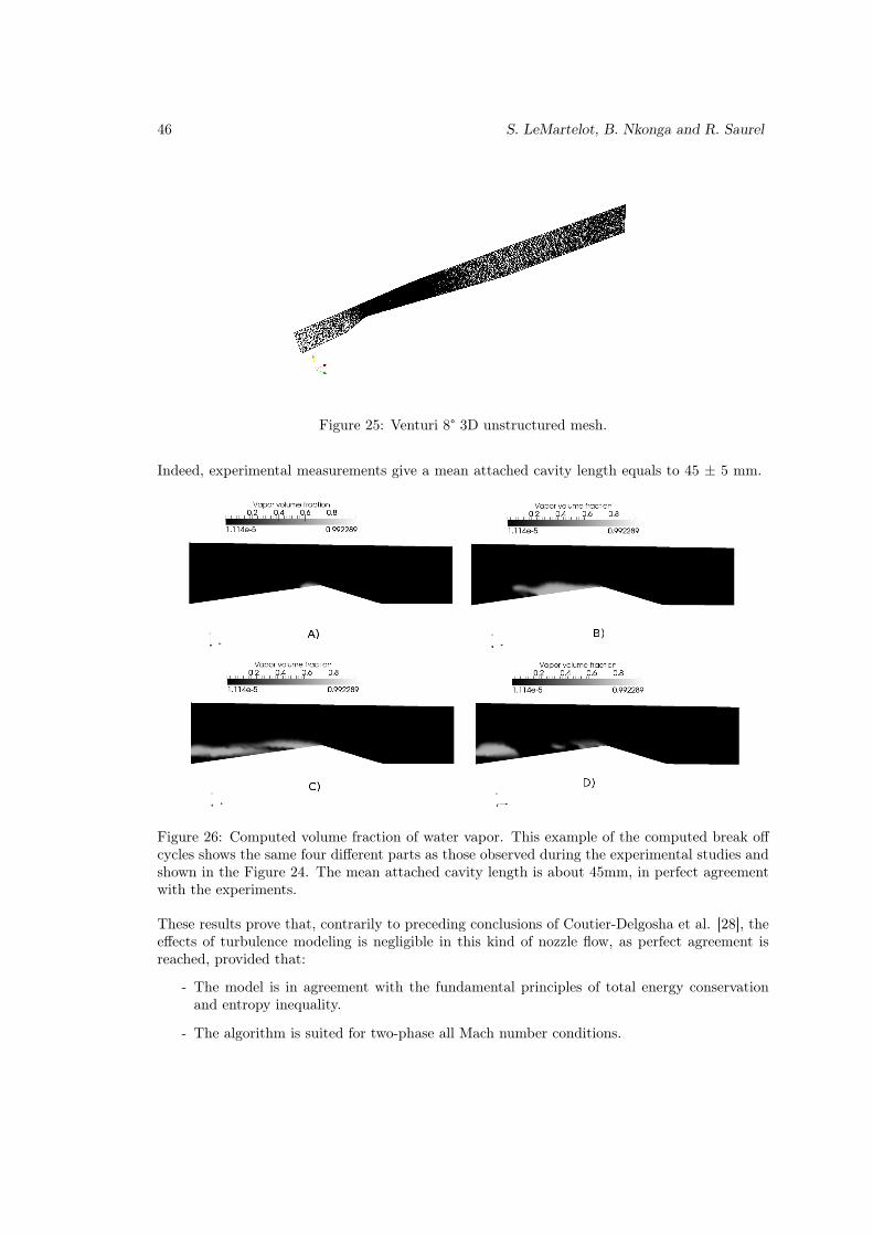
46 S. LeMartelot, B. Nkonga and R. Saurel
Figure 25: Venturi 8° 3D unstructured mesh.
Indeed, experimental measurements give a mean attached cavity length equals to 45 ± 5 mm.
Figure 26: Computed volume fraction of water vapor. This example of the computed break offcycles shows the same four different parts as those observed during the experimental studies andshown in the Figure 24. The mean attached cavity length is about 45mm, in perfect agreementwith the experiments.
These results prove that, contrarily to preceding conclusions of Coutier-Delgosha et al. [28], theeffects of turbulence modeling is negligible in this kind of nozzle flow, as perfect agreement isreached, provided that:
- The model is in agreement with the fundamental principles of total energy conservationand entropy inequality.
- The algorithm is suited for two-phase all Mach number conditions.

Liquid and liquid-gas flows at all speeds 47
Figure 27: Spectral analysis of the recorded pressure signal using a pressure jauge located at theend of the Venturi divergent. The obtained spectrum shows maximum intensity for frequenciesbetween 40 and 50 Hz. This is in excellent agreement with the observed cloud shedding frequencyof 43Hz and in excellent agreement with the experimental frequency of 45± 5 Hz.
6 Conclusion
The design of accurate numerical schemes require reference solutions. In the present paper,single phase and two-phase quasi one-dimensional steady state solutions have been obtained.They have been widely used to check the accuracy of preconditioned numerical schemes. TheTurkel preconditioned formulation has been used in the Riemann problem solution determinationand embedded in the Godunov method with HLLC scheme, in both explicit and implicit versions.This variant of the Turkel method, due to Guillard and Viozat [13], has shown particular efficiencyfor all Mach number single phase flow conditions. It has been extended to the two-phase flowmodel of Kapila et al [19], particularly suited for interfacial flows [38] as well as cavitating flows[39]. Compared to conventional cavitation model widely used in industry, this model is notbarotropic as it conserves energy. Also, phase transition is modeled in a thermodynamicallyconsistent way.
The preconditioning method requires mild modifications on the internal energy jumps condi-tions in the Riemann problem that have important consequences on method convergence. Themethod has been validated against exact 1D solutions and experimental 2D cavitating Venturiflows. Without using any adjustable parameter, perfect agreement has been obtained, contrarilyto previous attempts.

48 S. LeMartelot, B. Nkonga and R. Saurel
References
[1] R. Abgrall. How to prevent pressure oscillations in multicomponent flow calculations: Aquasi conservative approach. Journal of Computational Physics, 125:150–160, (1996).
[2] T. Alazard. Low Mach number limit of the full Navier-Stokes equations. Arch. Ration.Mech. Anal., 180(1):1–73, (2006).
[3] D.P. Babii, S.K.Godunov, V.T. Zhukov, and O.B. Feodoritova. On the different approxi-mations of overdetermined hyperbolic equations of classical mathematical physics. Comp.Mathematics and Mathematics Physics, 47(3):427–441, (2007).
[4] T.J. Barth and D.C. Jespersten. The design and application of upwind schemes on unstruc-tured meshes. Proceedings of the AIAA 27th Aerospace Sciences Meeting (Reno, Nevada),(1989).
[5] P. Birken and A. Meister. On low Mach number preconditioning of finite volume schemes.Proc. Appl. Math. Mech., 5:759–760, (2005).
[6] B. Braconnier and B. Nkonga. An all-speed relaxation scheme for interface flows with surfacetension. Journal of Computational Physics, 228(16):5722 – 5739, (2009).
[7] S.F. Davis. Simplified second-order Godunov-type methods. SIAM J. Sci. Statist. Comput.,9:445–473, (1988).
[8] D. G. Ebin. The motion of slightly compressible fluids viewed as a motion with strongconstraining force. Ann. of Math, 105(1):141–200, (1977).
[9] N. Favrie, S.L. Gavrilyuk, and R. Saurel. Solid-fluid diffuse interface model in cases ofextreme deformations. Journal of Computational Physics, 228(16):6037 – 6077, (2009).
[10] R. Fedkiw, Aslam T., Merriman B., and Osher S. A non-oscillatory Eulerian approachto interfaces in multimaterial flows (the Ghost Fluid Method). Journal of ComputationalPhysics, 152(2):457–492, (1999).
[11] J. Glimm, J.W. Grove, X.L. Li, K.M. Shyue, Q. Zhang, and Y. Zeng. Three dimensionalfront tracking. SIAM J. Scientific Computing, 19:703–727, (1998).
[12] H. Guillard and C. Viozat. On the behaviour of upwind schemes in the low mach numberlimit. Computers and Fluids, 28:63–86, (1999).
[13] H. Guillard and C. Viozat. On the behaviour of upwind schemes in the low mach numberlimit. Computers and Fluids, 28(1):63 – 86, (1999).
[14] F. Harlow and A. Amsden. Fluid dynamics. Monograph LA, Los Alamos National Labora-tory, Los Alamos,NM, LA-4700:1678–1712, (1971).
[15] F. Harlow and A. Amsden. A numerical fluid dynamics calculation method for all flowspeeds. Journal of Computational Physics, 8(2):197 – 213, (1971).
[16] A. Harten, P.D. Lax, and B. van Leer. On upstream differencing and Godunov-type schemesfor hyperbolic conservation laws. SIAM Rev., 25:35–61, (1983).
[17] C.W. Hirt and B.D. Nichols. Volume of fluid (VOF) method for the dynamics of freeboundaries. Journal of Computational Physics, 3:201–255, (1981).

Liquid and liquid-gas flows at all speeds 49
[18] D. Juric and G. Tryggvason. Computations of boiling flows. International Journal ofMultiphase Flow, 24(3):387 – 410, (1998).
[19] A.K. Kapila, R. Menikoff, J.B. Bdzil, S.F. Son, and D.S. Stewart. Two-phase modeling ofof deflagration-to-detonation transistion in granular materials: Reduced equations. Physicsof Fluids, 13:3002–3024, (2001).
[20] S. Klainerman and A. Majda. Singular limits of quasilinear hyperbolic systems with largeparameters and the incompressible limit of compressible fluids. Comm. Pure Appl. Math,34(4):481–524, (1981).
[21] S. Kokh and F. Lagoutière. An anti-diffusive numerical scheme for the simulation of inter-faces between compressible fluids by means of a five-equation model. Journal of Computa-tional Physics, 229(8):2773 – 2809, (2010).
[22] B. Lafaurie, C.Nardone, R. Scardovelli, S. Zaleski, and G. Zanetti. Modelling mergingand fragmentation in multiphase flows with SURFER. Journal of Computational Physics,113:134–147, (1994).
[23] DJ. Mavripilis. Revisiting the least-squares procedure for gradient reconstruction on un-structured meshes. AIAA 16th Computational Fluid Dynamics Conference, page 3986,(2003).
[24] T. Menard, S. Tanguy, and A. Berlemont. Coupling Level Set/VOF/Ghost Fluid methods.Validations and application to 3D simulation of the primary break-up of a liquid jet. Int.J. of Multiphase Flow, 33(5):510–524, (2007).
[25] R. Menikoff and B.J. Plohr. The Riemann problem for fluid flow of real materials. Rev.Mod. Phys., 61:75–130, (1989).
[26] G. Metivier and S. Schochet. The incompressible limit of the non-isentropic Euler equations.Arch. Ration. Mech. Anal., 158(1):61–90, (2001).
[27] O. Le Métayer, J. Massoni, and R. Saurel. Élaboration des lois d’état d’un liquide et desa vapeur pour les modèles d’écoulements diphasiques. International Journal of ThermalSciences, 43(3):265 – 276, (2004 (in French)).
[28] R. Fortes-Patella O. Coutier-Delgosha and J.L. Rebond. Evaluation of the turbulencemodel influence on the numerical simulations of unsteady cavitation. J. Fluid Engineer-ing, 125(1):38–45, (2003).
[29] G. Perigaud and R. Saurel. A compressible flow model with capillary effects. Journal ofComputational Physics, 209:139–178, (2005).
[30] F. Petitpas, E. Franquet, R. Saurel, and O. Le Metayer. A relaxation-projection methodfor compressible flows. Part II: Artificial heat exchanges for multiphase shocks. Journal ofComputational Physics, 225(2):2214 – 2248, (2007).
[31] F. Petitpas, J. Massoni, R. Saurel, E. Lapebie, and L. Munier. Diffuse interface modelfor high speed cavitating underwater systems. International Journal of Multiphase Flow,35(8):747 – 759, (2009).
[32] F. Petitpas, R. Saurel, E. Franquet, and A. Chinnayya. Modelling detonation waves in con-densed energetic materials : Multiphase CJ conditions and multidimensionnal computations.Shock Waves, 19:377–401, (2009).

50 S. LeMartelot, B. Nkonga and R. Saurel
[33] Y. Saad. Numerical methods for large eigenvalue problems. Manchester University Press,(1992).
[34] R. Saurel and R. Abgrall. A multiphase Godunov method for multifluid and multiphaseflows. Journal of Computational Physics, 150:425–467, (1999).
[35] R. Saurel, E. Franquet, E. Daniel, and O. Le Metayer. A relaxation-projection method forcompressible flows. Part I: The numerical equation of state for the Euler equations. Journalof Computational Physics, 223(2):822 – 845, (2007).
[36] R. Saurel, O. Le Metayer, J. Massoni, and S. Gavrilyuk. Shock jump relations for multiphasemixtures with stiff mechanical relaxation. Shock Waves, 16:209–232, (2007).
[37] R. Saurel, N.Favrie, F.Petitpas, M-H.Lallemand, and S.L. Gavrilyuk. Modelling dynamicand irreversible powder compaction. Journal of Fluid Mechanics, 664:348–396, (2010).
[38] R. Saurel, F. Petitpas, and R. A.Berry. Simple and efficient methods relaxation for inter-faces separating compressible fluids, cavitating flows and shocks in multiphase mixtures. J.Comput. Phys., 228:1678–1712, (2009).
[39] R. Saurel, F. Petitpas, and R. Abgrall. Modelling phase transition in metastable liquids:Application to cavitating and flashing flows. Journal of Fluid Mechanics, 607:313–350,(2008).
[40] S. Schochet. The compressible Euler equations in a bounded domain: Existence of solutionsand the incompressible limit. Comm. Math. Phys., 104(1):49–75, (1986).
[41] R. Shukla, C. Pantano, and J. Freund. An interface capturing method for the simulationof multi-phase compressible flows. Journal of Computational Physics, 229(19):7411 – 7439,(2010).
[42] E.F. Toro, M. Spruce, and W. Speares. Restoration of the contact surface in the HLL-Riemann solver. Shock Waves J., 4:25–34, (1994).
[43] E. Turkel. Preconditioned methods for solving the incompressible and low speed compress-ible equations. Journal of Computational Physics, 72(2):277 – 298, (1987).
[44] B. Van Leer. Towards the ultimate conservative difference scheme, V.A second order sequelto Godunov’s method. J. Comput. Phys., 32:445–473, (1979).
[45] A.B. Wood. A textbook of sound. Bell Eds, (1930).

Liquid and liquid-gas flows at all speeds 51
Appendix A -Godunov HLLC scheme for the Euler equations
in ducts of smooth varying cross sections
Consider a computational cell corresponding to an arbitrary control volume of the nozzle, asshow in the Figure 28 :
Figure 28: A computational cell i with its two cell boundaries, i+1/2 and i-1/2.
The conventional 1D Godunov scheme for ducts of smooth varying cross sections reads :
Un+1i = Un
i − ∆t
Vi
(
F ∗i+ 1
2
Si+ 1
2
− F ∗i− 1
2
Si− 1
2
)
+∆t
Vi
Gi
(
Si+ 1
2
− Si− 1
2
)
(135)
with
U =
ρ
ρu
ρE
F =
ρu
ρu2 + p
(ρE + p)u
Gi =
0pni0
Where :- U represents the conservative variables vector,- F represents the flux vector,- S represents the cell boundary surface,- Vi represents the cell volume .
The HLLC Riemann solver (Toro et al.) [42] is used to compute the intercell flux F ∗. At cellboundary i+ 1
2 , it reads:
FL,R =1
2(FL+FR)−sign(SL)
SL
2(U∗
L−UL)−sign(SM )SM
2(U∗
R−U∗L)−sign(SR)
SR
2(UR−U∗
R)
(136)

52 S. LeMartelot, B. Nkonga and R. Saurel
Figure 29: Schematization of the Euler equations Riemann problem under HLL approximationand associated wave speeds.
The subscripts L and R denote the left and right state of the Riemann problem, respectively.The wave speeds SR and SL are estimated with Davis approximation [7],
SR = Max(uR + cR, uL + cL) (137)
SL = Max(uR − cR, uL − cL) (138)
while SM is estimated under HLL [16] approximation :
SM =SRUR(2)− SLUL(2)− (FR(2)− FL(2))
SRUR(1)− SLUL(1)− (FR(1)− FL(1))(139)
The states U∗L and U∗
R are determined with the help of Rankine-Hugoniot jump relations acrossthe SR and SL waves,
F ∗L − SLU
∗L = FL − SLUL, (140)
F ∗R − SRU
∗R = FR − SRUR, (141)
and continuity relations : u∗L = u∗
R = SM and p∗L = p∗R = p∗:
U∗L =
1
SM − SL
[FL − SLUL − (0, p∗, SM .p∗)T ] (142)
U∗R =
1
SM − SR
[FR − SRUR − (0, p∗, SM .p∗)T ] (143)

Liquid and liquid-gas flows at all speeds 53
Appendix B -HLLC Riemann solver derivatives
The HLLC approximate Riemann solver is recalled hereafter:
FL,R =1
2(FL+FR)−sign(SL)
SL
2(U∗
L−UL)−sign(SM )SM
2(U∗
R−U∗L)−sign(SR)
SR
2(UR−U∗
R),
The flux vector derivatives are given by:
∂FLR
∂UL
=1
2
∂FL
∂UL
− sign(SL)SL
2(∂U∗
L
∂UL
− 1)− sign(SM )SM
2(∂(U∗
R − U∗L)
∂UL
) + sign(SR)SR
2(∂U∗
R
∂UL
)
(144)
∂FLR
∂UR
=1
2
∂FR
∂UR
− sign(SL)SL
2
∂U∗L
∂UR
− sign(SM )SM
2(∂(U∗
R − U∗L)
∂UR
)− sign(SR)SR
2(1− ∂U∗
R
∂UR
)
(145)Where :
U∗L =
1
SM − SL
[FL − SLUL − (0, P ∗, SM .P ∗)T ] (146)
U∗R =
1
SM − SR
[FR − SRUR − (0, P ∗, SM .P ∗)T ] (147)
∂U∗L
∂UL
=(∂FL
∂UL
− SL − ∂
∂UL
(0, P ∗, SM .P ∗)T )(SM − SL)− (FL − SLUL − (0, P ∗, SM .P ∗)T )∂SM
∂UL
(SM − SL)2
(148)
∂U∗L
∂UR
=− ∂
∂UL
((0, P ∗, SM .P ∗)T )(SM − SL)− (FL − SRUL − (0, P ∗, SM .P ∗)T )∂SM
∂UR
(SM − SL)2(149)
∂U∗R
∂UL
=− ∂
∂UL
((0, P ∗, SM .P ∗)T )(SM − SR)− (FR − SRUR − (0, P ∗, SM .P ∗)T )∂SM
∂UL
(SM − SR)2(150)
∂U∗R
∂UR
=(∂FR
∂UR
− SR − ∂
∂UR
(0, P ∗, SM .P ∗)T )(SM − SR)− (FR − SRUR − (0, P ∗, SM .P ∗)T )∂SM
∂UR
(SM − SR)2
(151)
Using Relations 140, 141, and P ∗L = P ∗
R = P ∗, two expressions for P ∗ are obtained:
P ∗ = FL(2)− SLUL(2)− SM (FL(1)− SLUL(1)) (152)
andP ∗ = FR(2)− SRUR(2)− SM (FR(1)− SRUR(1)) (153)

54 S. LeMartelot, B. Nkonga and R. Saurel
Nevertheless, in order to have a more precise derivative, the following average expression is usedfor P ∗:
P ∗ =FR(2)− SRUR(2)− SM (FR(1)− SRUR(1)) + FL(2)− SLUL(2)− SM (FL(1)− SLUL(1))
2(154)
∂P ∗
∂UL
=1
2
[
∂FL(2)
∂UL
− SL(0, 1, 0)T − SM
(
∂FL(1)
∂UL
− SL(1, 0, 0)T
)
− (FL(1)− SLUL(1))∂SM
∂UL
]
(155)
∂P ∗
∂UR
=1
2
[
∂FR(2)
∂UR
− SR(0, 1, 0)T − SM
(
∂FR(1)
∂UR
− SR(1, 0, 0)T
)
− (FR − SRUR)∂SM
∂UR
]
(156)
SM =SRUR(2)− SLUL(2)− (FR(2)− FL(2))
SRUR(1)− SLUL(1)− (FR(1)− FL(1))(157)
∂SM
∂UL
=(∂FL(2)
∂UL
− SL
∂UL(2)
∂UL
)(SRUR(1)− SLUL(1)− (FR(1)− FL(1)))
(SRUR(1)− SLUL(1)− (FR(1)− FL(1)))2
−(SRUR(2)− SLUL(2)− (FR(2)− FL(2)))(
∂FL(1)
∂UL
− SL
∂UL(1)
∂UL
)
(SRUR(1)− SLUL(1)− (FR(1)− FL(1)))2
(158)
∂SM
∂UR
=(SR
∂UR(2)
∂UR
− ∂FR(2)
∂UR
)(SRUR(1)− SLUL(1)− (FR(1)− FL(1)))
(SRUR(1)− SLUL(1)− (FR(1)− FL(1)))2
−(SRUR(2)− SLUL(2)− (FR(2)− FL(2)))(SR
∂UR(1)
∂UR
− ∂FR(1)
∂UR
)
(SRUR(1)− SLUL(1)− (FR(1)− FL(1)))2
(159)
These various derivatives require the knowledge of∂FL
∂UL
and∂FR
∂UR
. They correspond to the
Jacobian matrix of the Euler equations. In the single phase flow situation the pressure is givenby the Stiffened-Gas equation of state [14], [25], [27] :
P = (γ − 1)ρe− γP∞
With this EOS, the Jacobian matrix reads (with m = ρu and ξ = ρE) :
J =
0 1 0m2
2ρ2(γ − 3) (3− γ)
m
ργ - 1
-γmξ
ρ2+(γ − 1)
m3
ρ3+
mγP∞
ρ2γξ
ρ− 3
2
m2(γ − 1)
ρ2− γP∞
ρ
γm
ρ
Slight changes have to be done with the two phase flow model. They are detailed in the nextappendix.
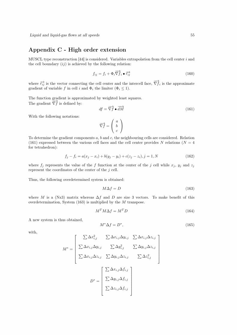
Liquid and liquid-gas flows at all speeds 55
Appendix C - High order extension
MUSCL type reconstruction [44] is considered. Variables extrapolation from the cell center i andthe cell boundary (ij) is achieved by the following relation:
fij = fi +Φi
−→∇f i • −→rij (160)
where −→rij is the vector connecting the cell center and the intercell face,−→∇f i is the approximate
gradient of variable f in cell i and Φi the limiter (Φi ≤ 1).
The function gradient is approximated by weighted least squares.The gradient
−→∇f is defined by:
df =−→∇f • −−→dM (161)
With the following notations:
−→∇f =
a
b
c
To determine the gradient components a, b and c, the neighbouring cells are considered. Relation(161) expressed between the various cell faces and the cell center provides N relations (N = 4for tetrahedron):
fj − fi = a(xj − xi) + b(yj − yi) + c(zj − zi), j = 1, N (162)
where fj represents the value of the f function at the center of the j cell while xj , yj and zjrepresent the coordinates of the center of the j cell.
Thus, the following overdetermined system is obtained:
M∆f = D (163)
where M is a (Nx3) matrix whereas ∆f and D are size 3 vectors. To make benefit of thisoverdetermination, System (163) is multiplied by the M transpose.
MTM∆f = MTD (164)
A new system is thus obtained,M∗∆f = D∗, (165)
with,
M∗ =
∑
∆x2i,j
∑
∆xi,j∆yi,j∑
∆xi,j∆zi,j
∑
∆xi,j∆yi,j∑
∆y2i,j∑
∆yi,j∆zi,j
∑
∆xi,j∆zi,j∑
∆yi,j∆zi,j∑
∆z2i,j
D∗ =
∑
∆xi,j∆fi,j
∑
∆yi,j∆fi,j
∑
∆zi,j∆fi,j

56 S. LeMartelot, B. Nkonga and R. Saurel
where :∆xi,j = xj − xi
∆yi,j = yj − yi∆zi,j = zj − zi∆fi,j = fj − fi
However, the matrix M∗ determinant can become very small if some cells are very close. Toovercome this situation, one way to proceed is to use weights. A very simple weighting procedurehas been proposed in [23]. It consists in modifying System (165) as follows:
M∗ =
∑
w2i,j∆x2
i,j
∑
w2i,j∆xi,j∆yi,j
∑
w2i,j∆xi,j∆zi,j
∑
w2i,j∆xi,j∆yi,j
∑
w2i,j∆y2i,j
∑
w2i,j∆yi,j∆zi,j
∑
w2i,j∆xi,j∆zi,j
∑
w2i,j∆yi,j∆zi,j
∑
w2i,j∆z2i,j
D∗ =
∑
w2i,j∆xi,j∆fi,j
∑
w2i,j∆yi,j∆fi,j
∑
w2i,j∆zi,j∆fi,j
where wi,j =1
√
∆x2i,j +∆y2i,j +∆z2i,j
.
This correction guarantees that the determinant of M∗ is O(1).
The last step in the higher order extension method deals with gradients limitation. The Barthand Jespersen [4] method is adopted. For each i cell, the gradient limitation of a f functionworks as follows:
Computations of the minimum and maximum of f such as,
fmax = max(fi, fj|j∈V o(i)),
andfmin = min(fi, fj|j∈V o(i)).
Then, for each neighbour j of i, the two following steps are achieved.The function Φi,j used in Equation (160) is determined as:-First compute Φi,j for each cell boundary as:
Φi,j =
min(1,fmin − fi
fij − fi), if (fi,j − fi) > 0
min(1,fmax − fi
fij − fi), if (fi,j − fi) < 0
1 if (fi,j − fi) = 0
- Then, Φi is computed as:Φi = min(Φi,j|j∈v(i)), (166)
Liquid and liquid-gas flows at all speeds 57
Appendix D -Mixture pressure derivatives
The mixture pressure for the two-phase non-equilibrium model reads:
P =
N∑
k=1
αkpk
where N is the number of fluids.With the help of the EOS (2) it becomes:
P =
N∑
k=1
[(γk − 1)αkρkek − αkγkP∞,k] (167)
The volume fraction of fluid N is determined from the saturation constraint :
αN = 1−N−1∑
k=1
αk
Thus, equation (167) becomes:
P =
N∑
k=1
(γk − 1)αkρkek +
N−1∑
k=1
αk(γNP∞,N − γkP∞,k)− γNP∞,N (168)
With the following derivatives:∂P
∂αkρkek= γk − 1
∂P
∂αk
= (γNP∞,N − γkP∞,k)
Appendix E -Implicit schemes for non-conservative equations
of the two-phase flow model
Volume fraction implicit scheme
In one-dimension, the volume fraction equation of System (5) reads:
∂α1
∂t+ u
∂α1
∂x= 0
The Godunov method for advection equations reads:
αn+11,i = αn
1,i +∆t
∆x
[
(
αn1,i−1 − αn
i
)
S+M,i− 1
2
−(
αn1,i+1 − αn
i
)
S−M,i+ 1
2
]
Where :SM represents the contact wave speed and
S+M,i− 1
2
=1
2
(
1 + sign(SM,i− 1
2
))
SM,i− 1
2
,
S−M,i+ 1
2
=1
2
(
1− sign(SM,i+ 1
2
))
SM,i+ 1
2
.

58 S. LeMartelot, B. Nkonga and R. Saurel
Let’s denote by:
fnLi =
(
αn1,i−1 − αn
i
)
S+M,i− 1
2
=(
1 + sign(SM,i− 1
2
))
(
αn1,i−1 − αn
i
)SM,i− 1
2
2
fnRi =
(
αn1,i+1 − αn
i
)
S−M,i+ 1
2
=(
1− sign(SM,i+ 1
2
))
(
αn1,i+1 − αn
i
)SM,i+ 1
2
2
Thus, the implicit scheme for the volume fraction equation reads:
αn+11,i = αn
1,i −∆t
∆x
[
fn+1Ri − fn+1
Li
]
(169)
It is worth to mention that fRi 6= fLi+1 as the equation is non-conservative.
Using the same development as previously (116 - 117), with δαi = αn+11,i − αn
1,i, the followingscheme is obtained,[
I +∆t
∆x
(
∂fRi
∂Ui
− ∂fLi
∂Ui
)]
δαi+∆t
∆x
∂fRi
∂Ui+1δαi+1−
∆t
∆x
∂fRi
∂Ui−1δαi−1 = −∆t
∆x(fn
Ri − fnLi) , (170)
where U is represents the whole conservative variables vector.
Internal energies implicit scheme
In one-dimension, the internal energy equations read (k = 1, 2):
∂αkρkek
∂t+
∂αkρkeku
∂x+ αkpk
∂u
∂x= 0 (171)
The explicit scheme used for this equation reads:
(αρe)n+1k = (αρe)
nk − ∆t
∆x
(
(αρeu)∗,n
k,i+ 1
2
− (αρeu)∗,n
k,i− 1
2
+ (αp)nk,i
(
u∗,n
i+ 1
2
− u∗,n
i− 1
2
))
(172)
where the product (αkpk)ni is assumed constant during the time step and the superscript ” ∗ ”
denotes the Riemann problem solution state .
Thus, the implicit scheme for the internal energy equations read:
(αρe)n+1k = (αρe)
nk − ∆t
∆x
(
(αρeu)∗,n+1
k,i+ 1
2
− (αρeu)∗,n+1
k,i− 1
2
+ (αp)n+1k,i
(
u∗,n+1
i+ 1
2
− u∗,n+1
i− 1
2
))
(173)
Using the same development as previously (116 - 117) with Fek = (αρeu)k and δ(αρe)k,o =(αρe)n+1
k,i − (αρe)nk,i, the following scheme is obtained:[
I +∆t
∆x
(
∂Fnek,i+ 1
2
∂Ui
−∂Fn
ek,i− 1
2
∂Ui
+ (αp)nk,i
[
∂u∗i+ 1
2
∂Ui
−∂u∗
i− 1
2
∂Ui
]
+ (u∗i+ 1
2
− u∗i− 1
2
)∂(αp)nk,i∂Ui
)]
δ(αρe)k,i
+∆t
∆x
[
∂Fek,i+ 1
2
∂Ui+1+ (αp)nk,i
∂u∗i+ 1
2
∂Ui+1
]
δ(αρe)k,i+1 −∆t
∆x
[
∂Fek,i− 1
2
∂Ui−1+ (αp)nk,i
∂u∗i− 1
2
∂Ui−1
]
δ(αρe)k,i−1
= −∆t
∆x
(
(αρeu)∗,n
k,i+ 1
2
− (αρeu)∗,n
k,i− 1
2
+ (αp)nk,i
(
u∗,n
i+ 1
2
− u∗,n
i− 1
2
))
(174)

Liquid and liquid-gas flows at all speeds 59
Where∂Fek,i+ 1
2
∂Ui
,∂Fek,i+ 1
2
∂Ui+1,∂Fek,i− 1
2
∂Ui
and∂Fek,i− 1
2
∂Ui−1are calculated using the HLLC flux deriva-
tives (Appendix 6 ).
Appendix F -Stiff thermodynamic relaxation
A two-phase liquid, vapor mixture in thermodynamic equilibrium is considered. Both phases arethus in pressure, temperature and Gibbs free energy equilibrium.The thermodynamic equilibrium state is determined by considering the following algebraic sys-tem:
v =1
ρ= Y1v1 + Y2v2 = cte = v0
e = Y1e1 + Y2e2 = cte = e0
T1 = T2 = T
p1 = p2 = p
g1 = g2
(175)
Where Y1 =α1ρ1
ρand Y2 =
α2ρ2
ρ= 1− Y1 denote the mass fractions of both phases, which are
not constant during the relaxation process.The first two equations of this system come from the mass conservation and mixture totalenergy conservation, respectively. The last equation represents the Gibbs free energies equality(g = h− Ts).The liquid and its vapor are denoted by the subscripts "1" and "2", respectively.The specific volumes and the internal energies of each phase are given by the following expressions,based on the stiffened gas EOS (2):
vk =(γk − 1)Cv,kTk
pk + p∞,k
(176)
ek = Cv,kTk(1 +(γk − 1)p∞,k
p+ p∞,k
) + qk (177)
Each parameter involved in the previous expressions (γk, Cv,k, p∞,k, qk) is calculated in order tofit the liquid-vapor phase diagram, more precisely the corresponding saturation curves. Detailsregarding the EOS parameters determination are given in [27] and [39].Denoting the final state by the superscript ’*’, the mass conservation constraint becomes:
v0 = Y ∗1 v
∗1(p
∗) + Y ∗2 v
∗2(p
∗) = Y ∗1 v
∗1(p
∗) + (1− Y ∗1 )v
∗2(p
∗), (178)
with v∗1(p∗) =
(γk − 1)Cv,kT∗(p∗)
p∗ + p∞,k
.
Constraints of pressures, temperatures and Gibbs free energies equilibrium have been used inRelation (178). Indeed, the Gibbs free energies equality leads to a relationship between thepressure and the temperature:
T ∗(p∗) = Tsat(p∗) (179)
v∗1(p∗) and v∗2(p
∗) represent the saturated specific volumes of both phases. A first relation linkingthe liquid mass fraction and the pressure is thus obtained:
Y ∗1 =
v∗2(p∗)− v0
v∗2(p∗)− v∗1(p
∗)(180)

60 S. LeMartelot, B. Nkonga and R. Saurel
Consider now the mixture total energy conservation:
e0 = Y ∗1 e
∗1(p
∗) + Y ∗2 e
∗2(p
∗) = Y ∗1 e
∗1(p
∗) + (1− Y ∗1 )e
∗2(p
∗) (181)
with ek(p∗) = Cv,kT
∗k (p
∗)(1 +(γk − 1)p∞,k
p+ p∞,k
) + qk
A second relation linking the liquid mass fraction and the pressure is thus obtained:
Y ∗1 =
e0 − e∗2(p∗)
e∗1(p∗)− e∗2(p
∗)(182)
This relation can be also expressed as a function of the specific enthalpies of each phase:
Y ∗1 =
h∗2(p
∗)− (e0 − p∗v0)
h∗2(p
∗)− h∗1(p
∗)(183)
Where h1 and h2 are linked by h∗2(p
∗)− h∗1(p
∗) = Lv(p∗), Lv(p
∗) representing the latent heat ofvaporization, which is a function of the pressure.From the previous mass fraction equations, a single function of the pressure is obtained:
h∗2(p
∗)− (e0 − p∗v0)
h∗2(p
∗)− h∗1(p
∗)− v∗2(p
∗)− v0
v∗2(p∗)− v∗1(p
∗)= 0 (184)
Its solution is computed with the Newton method. Once the relaxed pressure is known, solutionof this equation is determined, the remaining variables are easily determined with the precedingthermodynamic relations.
Contents
1 Introduction 4
2 Flow Models 6
3 Reference solutions 83.1 Single phase nozzle flow . . . . . . . . . . . . . . . . . . . . . . . . . . . . . . . . 9
3.1.1 Critical pressure ratios . . . . . . . . . . . . . . . . . . . . . . . . . . . . . 93.1.2 Derivation of the Nozzle flow profile : Single phase Isentropic . . . . . . . 113.1.3 Derivation of the Nozzle flow profile : Single phase Adiabatic . . . . . . . 123.1.4 Solution examples . . . . . . . . . . . . . . . . . . . . . . . . . . . . . . . 123.1.5 Exact 1D nozzle solution with imposed mass flow rate and stagnation en-
thalpy . . . . . . . . . . . . . . . . . . . . . . . . . . . . . . . . . . . . . . 133.1.6 Comparison of the low Mach number compressible exact solution and the
incompressible exact one . . . . . . . . . . . . . . . . . . . . . . . . . . . . 143.1.7 Behavior of conventional Godunov type schemes in low Mach number con-
ditions . . . . . . . . . . . . . . . . . . . . . . . . . . . . . . . . . . . . . . 173.2 Two-phase nozzle flows . . . . . . . . . . . . . . . . . . . . . . . . . . . . . . . . . 17
3.2.1 Critical pressure ratios . . . . . . . . . . . . . . . . . . . . . . . . . . . . . 183.2.2 Derivation of the Nozzle flow profile : two-phase isentropic . . . . . . . . 223.2.3 Derivation of the Nozzle flow profile : two-phase Adiabatic . . . . . . . . 223.2.4 Solution examples . . . . . . . . . . . . . . . . . . . . . . . . . . . . . . . 233.2.5 Exact two-phase nozzle solution with imposed mass flow rate and stagna-
tion enthalpy . . . . . . . . . . . . . . . . . . . . . . . . . . . . . . . . . . 23
Liquid and liquid-gas flows at all speeds 61
4 Improving numerical convergence in the low Mach number limit 274.1 Low Mach number preconditioning . . . . . . . . . . . . . . . . . . . . . . . . . . 27
4.1.1 Dimensionless variables . . . . . . . . . . . . . . . . . . . . . . . . . . . . 284.1.2 Asymptotic analysis . . . . . . . . . . . . . . . . . . . . . . . . . . . . . . 284.1.3 System considered for the Riemann problem . . . . . . . . . . . . . . . . . 294.1.4 Two-phase low Mach preconditioning . . . . . . . . . . . . . . . . . . . . . 30
4.2 Preconditionned Riemann solvers illustrations . . . . . . . . . . . . . . . . . . . . 324.2.1 Single phase nozzle flow . . . . . . . . . . . . . . . . . . . . . . . . . . . . 324.2.2 Two phase nozzle flow . . . . . . . . . . . . . . . . . . . . . . . . . . . . . 324.2.3 Preconditioning method precautions . . . . . . . . . . . . . . . . . . . . . 34
4.3 Implicit scheme for the Euler equations . . . . . . . . . . . . . . . . . . . . . . . 374.3.1 Implicit Godunov scheme . . . . . . . . . . . . . . . . . . . . . . . . . . . 374.3.2 Flux derivatives . . . . . . . . . . . . . . . . . . . . . . . . . . . . . . . . . 384.3.3 Illustrations . . . . . . . . . . . . . . . . . . . . . . . . . . . . . . . . . . . 39
4.4 Multi-D extension . . . . . . . . . . . . . . . . . . . . . . . . . . . . . . . . . . . 404.5 Implicit scheme for the two-phase flow model . . . . . . . . . . . . . . . . . . . . 41
5 Illustrations and validations 425.1 One dimensional two-phase nozzle flow . . . . . . . . . . . . . . . . . . . . . . . . 425.2 3D Computations of cavitating flows in Venturi channels . . . . . . . . . . . . . . 44
5.2.1 Test case presentation . . . . . . . . . . . . . . . . . . . . . . . . . . . . . 445.2.2 Experimental results . . . . . . . . . . . . . . . . . . . . . . . . . . . . . . 455.2.3 Numerical results . . . . . . . . . . . . . . . . . . . . . . . . . . . . . . . . 45
6 Conclusion 47
References 47
Appendix 51

RESEARCH CENTRE
SOPHIA ANTIPOLIS – MÉDITERRANÉE
2004 route des Lucioles - BP 93
06902 Sophia Antipolis Cedex
Publisher
Inria
Domaine de Voluceau - Rocquencourt
BP 105 - 78153 Le Chesnay Cedex
inria.fr
ISSN 0249-6399