handheld multi-frame super-resolution · 2019-08-23 · handheld multi-frame super-resolution •...

Handheld Multi-Frame Super-Resolution

BARTLOMIEJWRONSKI, IGNACIOGARCIA-DORADO,MANFREDERNST, DAMIENKELLY,MICHAELKRAININ, CHIA-KAI LIANG, MARC LEVOY, and PEYMAN MILANFAR, Google Research

Fig. 1. We present a multi-frame super-resolution algorithm that supplants the need for demosaicing in a camera pipeline by merging a burst of raw images.

We show a comparison to a method that merges frames containing the same-color channels together first, and is then followed by demosaicing (top). By

contrast, our method (bottom) creates the full RGB directly from a burst of raw images. This burst was captured with a hand-held mobile phone and processed

on device. Note in the third (red) inset that the demosaiced result exhibits aliasing (Moiré), while our result takes advantage of this aliasing, which changes on

every frame in the burst, to produce a merged result in which the aliasing is gone but the cloth texture becomes visible.

Compared to DSLR cameras, smartphone cameras have smaller sensors,

which limits their spatial resolution; smaller apertures, which limits their

light gathering ability; and smaller pixels, which reduces their signal-to-

noise ratio. The use of color filter arrays (CFAs) requires demosaicing, which

further degrades resolution. In this paper, we supplant the use of traditional

demosaicing in single-frame and burst photography pipelines with a multi-

frame super-resolution algorithm that creates a complete RGB image directly

from a burst of CFA raw images. We harness natural hand tremor, typical in

handheld photography, to acquire a burst of raw frames with small offsets.

These frames are then aligned and merged to form a single image with red,

green, and blue values at every pixel site. This approach, which includes no

explicit demosaicing step, serves to both increase image resolution and boost

signal to noise ratio. Our algorithm is robust to challenging scene conditions:

local motion, occlusion, or scene changes. It runs at 100 milliseconds per

12-megapixel RAW input burst frame on mass-produced mobile phones.

Specifically, the algorithm is the basis of the Super-Res Zoom feature, as well

as the default merge method in Night Sight mode (whether zooming or not)

on Google’s flagship phone.

Authors’ address: Bartlomiej Wronski, [email protected]; Ignacio Garcia-Dorado, [email protected]; Manfred Ernst, [email protected]; Damien Kelly,[email protected]; Michael Krainin, [email protected]; Chia-Kai Liang,[email protected]; Marc Levoy, [email protected]; Peyman Milanfar, [email protected] Google Research, 1600 Amphitheatre Parkway, Mountain View, CA, 94043.

Permission to make digital or hard copies of part or all of this work for personal orclassroom use is granted without fee provided that copies are not made or distributedfor profit or commercial advantage and that copies bear this notice and the full citationon the first page. Copyrights for third-party components of this work must be honored.For all other uses, contact the owner/author(s).

© 2019 Copyright held by the owner/author(s).0730-0301/2019/7-ART28https://doi.org/10.1145/3306346.3323024

CCS Concepts: · Computing methodologies → Computational pho-

tography; Image processing.

Additional Key Words and Phrases: computational photography, super-

resolution, image processing, photography

ACM Reference Format:

Bartlomiej Wronski, Ignacio Garcia-Dorado, Manfred Ernst, Damien Kelly,

Michael Krainin, Chia-Kai Liang, Marc Levoy, and Peyman Milanfar. 2019.

Handheld Multi-Frame Super-Resolution. ACM Trans. Graph. 38, 4, Article 28

(July 2019), 18 pages. https://doi.org/10.1145/3306346.3323024

1 INTRODUCTION

Smartphone camera technology has advanced to the point that tak-ing pictures with a smartphone has become the most popular formof photography [CIPA 2018; Flickr 2017]. Smartphone photographyoffers high portability and convenience, but many challenges stillexist in the hardware and software design of a smartphone cam-era that must be overcome to enable it to compete with dedicatedcameras.Foremost among these challenges is limited spatial resolution.

The resolution produced by digital image sensors is limited not onlyby the physical pixel count (e.g., 12-megapixel camera), but also bythe presence of color filter arrays (CFA)1 like the Bayer CFA [Bayer1976]. Given that human vision is more sensitive to green, a quadof pixels in the sensor usually follows the Bayer pattern RGGB;i.e., 50% green, 25% red, and 25% blue. The final full-color image isgenerated from the spatially undersampled color channels throughan interpolation process called demosaicing [Li et al. 2008].

1Also known as a color filter mosaic (CFM).

ACM Trans. Graph., Vol. 38, No. 4, Article 28. Publication date: July 2019.

https://doi.org/10.1145/3306346.3323024

https://doi.org/10.1145/3306346.3323024

28:2 • Wronski et al.

Demosaicing algorithms operate on the assumption that the colorof an area in a given image is relatively constant. Under this as-sumption, the color channels are highly correlated, and the aimof demosaicing is to reconstruct the undersampled color informa-tion while avoiding the introduction of any visual artifacts. Typicalartifacts of demosaicing include false color artifacts such as chro-matic aliases, zippering (abrupt or unnatural changes of intensityover consecutive pixels that look like a zipper), maze, false gradient,and Moiré patterns (Figure 1 top). Often, the challenge in effectivedemosaicing is trading off resolution and detail recovery againstintroducing visual artifacts. In some cases, the underlying assump-tion of cross-channel correlation is violated, resulting in reducedresolution and loss of details.

A significant advancement in smartphone camera technology inrecent years has been the application of software-based computa-tional photography techniques to overcome limitations in camerahardware design. Examples include techniques for increasing dy-namic range [Hasinoff et al. 2016], improving signal-to-noise ratiothrough denoising [Godard et al. 2018; Mildenhall et al. 2018] andwide aperture effects to synthesize shallow depth-of-field [Wadhwaet al. 2018]. Many of these recent advancements have been achievedthrough the introduction of burst processing2 where on a shutterpress multiple acquired images are combined to produce a photothat is of greater quality than that of a single acquired image.In this paper, we introduce an algorithm that uses signals cap-

tured across multiple shifted frames to produce higher resolutionimages (Figure 1 bottom). Although the underlying techniques canbe generalized to any shifted signals, in this work we focus on ap-plying the algorithm to the task of resolution enhancement anddenoising in a smartphone image acquisition pipeline using burstprocessing. By using a multi-frame pipeline and combining differentundersampled and shifted information present in different frames,we remove the need for an explicit demosaicing step.

To work on a smartphone camera, any such algorithm must:

• Work handheld from a single shutter press ś without atripod or deliberate motion of the camera by the user.

• Run at an interactive rate ś the algorithm should producethe final enhanced resolution with low latency (within atmost a few seconds).

• Be robust to local motion and scene changes ś usersmight capture sceneswith fastmoving objects or scene changes.While the algorithm might not increase resolution in all suchscenarios, it should not produce appreciable artifacts.

• Be robust to noisy input data ś in low light the algorithmshould not amplify noise, and should strive to reduce it.

With these criteria in mind, we have developed an algorithm thatprocesses multiple successively captured raw frames in an onlinefashion. The algorithm tackles the tasks of demosaicing and super-resolution jointly and formulates the problem as the reconstructionand interpolation of a continuous signal from a set of sparse samples.Red, green and blue pixels are treated as separate signals on differentplanes and reconstructed simultaneously. This approach enables the

2We use the terms multi-frame and burst processing interchangeably to refer to theprocess of generating a single image from multiple images captured in rapid succession.

production of highly detailed images even when there is no cross-channel correlation ś as in the case of saturated single-channelcolors. The algorithm requires no special capturing conditions; nat-ural hand-motion produces offsets that are sufficiently random inthe subpixel domain to apply multi-frame super-resolution. Addi-tionally, since our super-resolution approach creates a continuousrepresentation of the input, it allows us to directly create an imagewith a desired target magnification / zoom factor without the needfor additional resampling. The algorithm works on a mobile deviceand incurs a computational cost of only 100 ms per 12-megapixelprocessed frame.

The main contributions of this work are:

(1) Replacing raw image demosaicing with a multi-frame super-resolution algorithm.

(2) The introduction of an adaptive kernel interpolation / mergemethod from sparse samples (Section 5) that takes into ac-count the local structure of the image, and adapts accordingly.

(3) A motion robustness model (Section 5.2) that allows the algo-rithm to work with bursts containing local motion, disocclu-sions, and alignment/registration failures (Figure 12).

(4) The analysis of natural hand tremor as the source of subpixelcoverage sufficient for super-resolution (Section 4).

2 BACKGROUND

2.1 Demosaicing

Demosaicing has been studied extensively [Li et al. 2008], and theliterature presents a wide range of algorithms. Most methods inter-polate the missing green pixels first (since they have double sam-pling density) and reconstruct the red and blue pixel values usingcolor ratio [Lukac and Plataniotis 2004] or color difference [Hi-rakawa and Parks 2006]. Other approaches work in the frequencydomain [Leung et al. 2011], residual space [Monno et al. 2015], useLAB homogeneity metrics [Hirakawa and Parks 2005] or non localapproaches [Duran and Buades 2014]. More recent works use CNNsto solve the demosaicing problem such as the joint demosaicing anddenoising technique by Gharbi et al. [2016]. Their key insight is tocreate a better training set by defining metrics and techniques formining difficult patches from community photographs.

2.2 Multi-frame Super-resolution (SR)

Single-image approaches exploit strong priors or training data. Theycan suppress aliasing3 well, but are often limited in how much theycan reconstruct from aliasing. In contrast to single frame techniques,the goal of multi-frame super-resolution is to increase the true(optical) resolution.

In the sampling theory literature, multi-frame super-resolutiontechniques date as far back as the ’50s [Yen 1956] and the ’70s [Pa-poulis 1977]. The work of Tsai [1984] started the modern conceptof super-resolution by showing that it was possible to improveresolution by registering and fusing multiple aliased images. Iraniand Peleg [1991], and then Elad and Feuer [1997] formulated the

3In this work we refer to aliasing in signal processing terms ś a signal with frequencycontent above half of the sampling rate that manifests as a lower frequency aftersampling [Nyquist 1928].


Handheld Multi-Frame Super-Resolution • 28:3

a) RAW Input Burst

b) Local Gradients

d) Alignment Vectors

e) Local Statistics

c) Kernels

f) Motion Robustness

g) Accumulation

h) Merged Result

Fig. 2. Overview of our method: A captured burst of raw (Bayer CFA) images (a) is the input to our algorithm. Every frame is aligned locally (d) to a single

frame, called the base frame. We estimate each frame’s contribution at every pixel through kernel regression (Section 5.1). These contributions are accumulated

separately per color channel (g). The kernel shapes (c) are adjusted based on the estimated local gradients (b) and the sample contributions are weighted

based on a robustness model (f) (Section 5.2). This robustness model computes a per-pixel weight for every frame using the alignment field (d) and local

statistics (e) gathered from the neighborhood around each pixel. The final merged RGB image (h) is obtained by normalizing the accumulated results per

channel. We call the steps depicted in (b)-(g) the merge.

algorithmic side of super-resolution. The need for accurate sub-pixel registration, existence of aliasing, and good signal-to-noiselevels were identified as the main requirements of practical super-resolution [Baker and Kanade 2002; Robinson and Milanfar 2004,2006].

In the early 2000s, Farsiu et al. [2006] andGotoh andOkutomi [2004]formulated super-resolution from arbitrary motion as an optimiza-tion problem that would be infeasible for interactive rates. Ben-Ezraet al. [2005] created a jitter camera prototype to do super-resolutionusing controlled subpixel detector shifts. This and other works in-spired some commercial cameras (e.g., Sony A6000, Pentax FF K1,Olympus OM-D E-M1 or Panasonic Lumix DC-G9) to adopt multi-frame techniques, using controlled pixel shifting of the physicalsensor. However, these approaches require the use of a tripod or astatic scene. Video super-resolution approaches [Belekos et al. 2010;Liu and Sun 2011; Sajjadi et al. 2018] counter those limitations andextend the idea of multi-frame super-resolution to video sequences.

2.3 Kernel Based Super-resolution and Interpolation

Takeda et al. [2006; 2007] formulated super-resolution as a kernelregression and reconstruction problem, which allows for faster pro-cessing. Around the same time, Müller et al. [2005] introduced atechnique to model fluid-fluid interactions that can be rendered us-ing kernel methods introduced by Blinn [1982]. Yu and Turk [2013]proposed an adaptive solution to the reconstructing of surfaces ofparticle-based fluids using anisotropic kernels. These kernels, likeTakeda et al. ’s, are based on local gradient Principal ComponentAnalysis (PCA), where the anisotropy of the kernels allows for si-multaneous preservation of sharp features and smooth rendering offlat surfaces. Similar adaptive kernel based method were proposed

for single image super-resolution by Hunt [2004] and for generalupscaling and interpolation by Lee and Yoon [2010]. We adopt someof these ideas and generalize them to fit our use case.

2.4 Burst Photography and Raw Fusion

Burst fusion methods based on raw imagery are relatively uncom-mon in the literature, as they require knowledge of the photographicpipeline [Farsiu et al. 2006; Gotoh and Okutomi 2004; Heide et al.2014; Wu and Zhang 2006]. Vandewalle et al. [2007] described an al-gorithm where information from multiple Bayer frames is separatedinto luminance and chrominance components and fused together toimprove the CFA demosaicing. Most relevant to our work is Hasinoffet al. [2016] which introduced an end-to-end burst photographypipeline fusing multiple frames for increased dynamic range andsignal-to-noise ratio. Our paper is a more general fusion approachthat (a) dispenses with demosaicing, (b) produces increased reso-lution, and (c) enables merging onto an arbitrary grid, allowingfor high quality digital zoom at modest factors (Section 7). Mostrecently, Li et al. [2018] proposed an optimization based algorithmfor forming an RGB image directly from fused, unregistered rawframes.

2.5 Multi-frame Rendering

This work also draws on multi-frame and temporal super-resolutiontechniques widely used in real-time rendering (for example, in videogames). Herzog et al. combined information from multiple renderedframes to increase resolution [2010]. Sousa et al. [2011] mentionedthe first commercial use of robustly combining information from twoframes in real-time in a video game, while Malan [2012] expandedits use to produce a 1920 × 1080 image from four 1280 × 720 frames.



Subsequent work [Drobot 2014; Karis 2014; Sousa 2013] establishedtemporal super-resolution techniques as state-of-the-art and stan-dard in real-time rendering for various effects, including dynamicresolution rendering and temporal denoising. Salvi [2016] provided atheoretical explanation of commonly used local color neighborhoodclipping techniques and proposed an alternative based on statisticalanalysis. While most of those ideas are used in a different context,we generalize their insights about detecting aliasing, misalignmentand occlusion in our robustness model.

2.6 Natural Hand Tremor

While holding a camera (or any object), a natural, involuntary handtremor is always present. The tremor is comprised of low amplitudeand high frequency motion components that occur while holdingsteady limb postures [Schäfer 1886]. The movement is highly peri-odic, with a frequency in the range of 8ś12 Hz, and its movement issmall in magnitude but random [Marshall and Walsh 1956]. The mo-tion also consists of amechanical-reflex component that depends onthe limb, and a second component that causes micro-contractions inthe limb muscles [Riviere et al. 1998]. This behavior has been shownto not change with age [Sturman et al. 2005] but it can change dueto disease [NIH 2018]. In this paper, we show that the hand tremorof a user holding a mobile camera is sufficient to provide subpixelcoverage for super-resolution.

3 OVERVIEW OF OUR METHOD

Our approach is visualized in Figure 2. First, a burst of raw (CFABayer) images is captured. For every captured frame, we align itlocally with a single frame from the burst (called the base frame).Next, we estimate each frame’s local contributions through kernelregression (Section 5.1) and accumulate those contributions acrossthe entire burst. The contributions are accumulated separately percolor plane. We adjust kernel shapes based on the estimated signalfeatures and weight the sample contributions based on a robustnessmodel (Section 5.2).We perform per-channel normalization to obtainthe final merged RGB image.

3.1 Frame Acquisition

Since our algorithm is designed to work within a typical burst pro-cessing pipeline, it is important that the processing does not increasethe overall photo capture latency. Typically, a smartphone operatesin a mode called Zero-Shutter Lag, where raw frames are beingcaptured continuously to a ring buffer when the user opens andoperates the camera application. On a shutter press, the most recentcaptured frames are sent to the camera processing pipeline. Our al-gorithm operates on an input burst (Figure 2 (a)) formed from thoseimages. Relying on previously captured frames creates challengesfor the super-resolution algorithm ś the user can be freely movingthe camera prior to the capture. The merge process must be ableto deal with natural hand motion (Section 4) and cannot requireadditional movement or user actions.

3.2 Frame Registration and Alignment

Prior to combining frames, we place them into a common coordinatesystem by registering frames against the base frame to create a set

of alignment vectors (Figure 2 (d)). Our alignment solution is arefined version of the algorithm used by Hasinoff et al. [2016]. Thecore alignment algorithm is coarse-to-fine, pyramid-based blockmatching that creates a pyramid representation of every input frameand performs a limited window search to find the most similar tile.Through the alignment process we obtain per patch/tile (with tilesizes of Ts ) alignment vectors relative to the base frame.

Unlike Hasinoff et al. [2016], we require subpixel accurate align-ment to achieve super-resolution. To address this issue we could usea different, dedicated registration algorithm designed for accuratesubpixel estimation (e.g., Fleet and Jepson [1990]), or refine the blockmatching results. We opted for the latter due to its simplicity andcomputational efficency. We have explored estimating the subpixeloffsets by fitting a quadratic curve to the block matching align-ment error and finding its minimum [Kanade and Okutomi 1991];however, we found that super-resolution requires a more accuratemethod. Therefore, we refine the block matching alignment vectorsby three iterations of Lucas-Kanade [1981] optical flow image warp-ing. This approach reached the necessary accuracy while keepingthe computational cost low.

3.3 Merge Process

After frames are aligned, the remainder of the merge process (Fig-ure 2 (b-g)) is responsible for fusing the raw frames into a full RGBimage. These steps constitute the core of our algorithm and will bedescribed in greater detail in Section 5.The merge algorithm works in an online fashion, sequentially

computing the contributions of each processed frame to every out-put pixel by accumulating colors from a 3 × 3 neighborhood. Thosecontributions are weighted by kernel weights (Section 5.1, Figure 2(c)), modulated by the robustness mask (Section 5.2, Figure 2 (f)),and summed together separately for the red, green and blue colorplanes. At the end of the process, we divide the accumulated colorcontributions by the accumulated weights, obtaining three colorplanes.The result of the merge process is a full RGB image, which can

be defined at any desired resolution. This can be processed furtherby the typical camera pipeline (spatial denoising, color correction,tone-mapping, sharpening) or alternatively saved for further offlineprocessing in a non-CFA raw format like Linear DNG [Adobe 2012].

Before we explain the algorithm details, we analyze the key char-acteristics that enable the hand-held super-resolution.

4 HAND-HELD SUPER-RESOLUTION

Multi-frame super-resolution requires two conditions to be ful-filled [Tsai and Huang 1984]:

(1) Input frames need to be aliased, i.e., contain high frequen-cies that manifest themselves as false low frequencies aftersampling.

(2) The input must contain multiple aliased images, sampledat different subpixel offsets. This will manifest as differentphases of false low frequencies in the input frames.

Having multiple lower resolution shifted and aliased images allowsus to both remove the effects of aliasing in low frequencies as wellas reconstruct the high frequencies. In a (mobile) camera pipeline,



-1.5 -1 -0.5 0 0.5 1 1.5

Horiztonal Angular Displacement (radians 10-3)

-1.5

-1

-0.5

0

0.5

1

1.5

Vert

ical A

ngula

r D

ispla

cem

ent (r

adia

ns

10

-3)

0 0.05 0.1 0.15 0.2 0.25 0.3 0.35

Angular Velocity (radians/sec)

0

0.05

0.1

0.15

0.2

Bin

Count / T

ota

l C

ount

a) b)

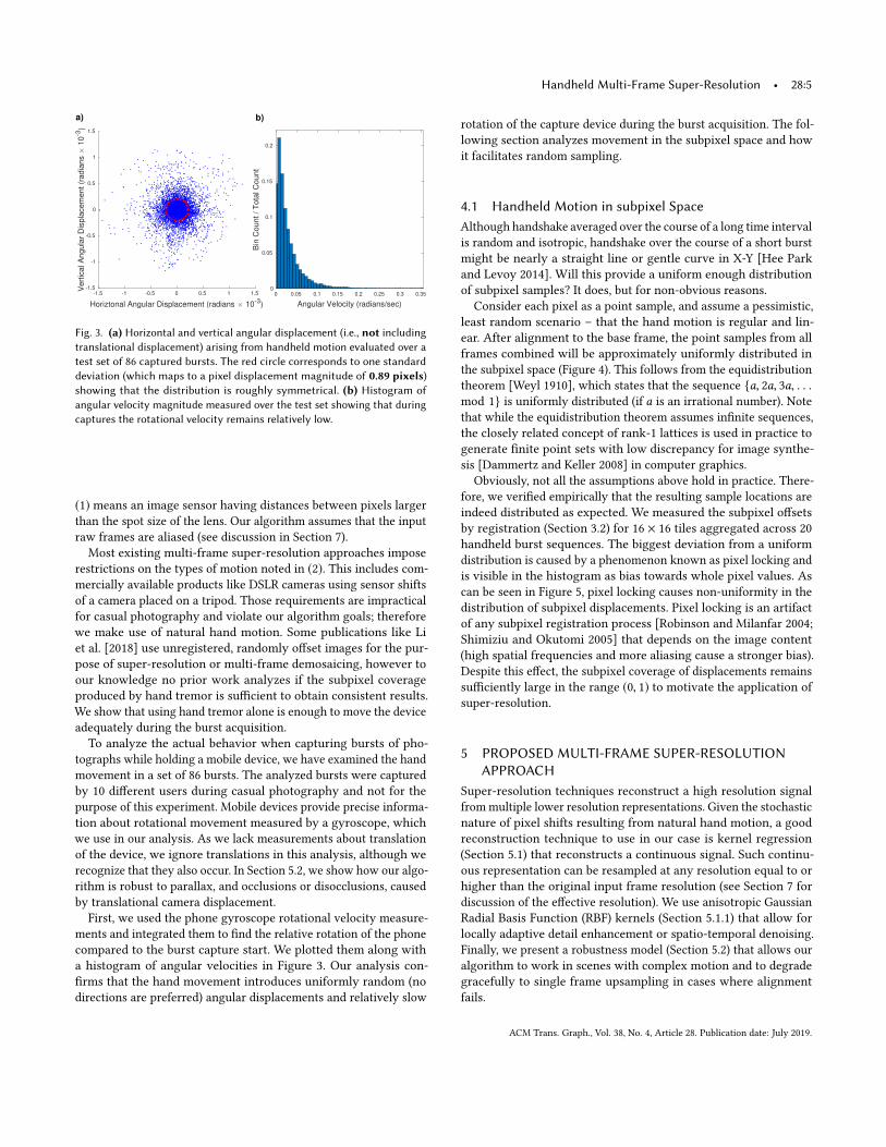
Fig. 3. (a) Horizontal and vertical angular displacement (i.e., not including

translational displacement) arising from handheld motion evaluated over a

test set of 86 captured bursts. The red circle corresponds to one standard

deviation (which maps to a pixel displacement magnitude of 0.89 pixels)

showing that the distribution is roughly symmetrical. (b) Histogram of

angular velocity magnitude measured over the test set showing that during

captures the rotational velocity remains relatively low.

(1) means an image sensor having distances between pixels largerthan the spot size of the lens. Our algorithm assumes that the inputraw frames are aliased (see discussion in Section 7).Most existing multi-frame super-resolution approaches impose

restrictions on the types of motion noted in (2). This includes com-mercially available products like DSLR cameras using sensor shiftsof a camera placed on a tripod. Those requirements are impracticalfor casual photography and violate our algorithm goals; thereforewe make use of natural hand motion. Some publications like Liet al. [2018] use unregistered, randomly offset images for the pur-pose of super-resolution or multi-frame demosaicing, however toour knowledge no prior work analyzes if the subpixel coverageproduced by hand tremor is sufficient to obtain consistent results.We show that using hand tremor alone is enough to move the deviceadequately during the burst acquisition.To analyze the actual behavior when capturing bursts of pho-

tographs while holding a mobile device, we have examined the handmovement in a set of 86 bursts. The analyzed bursts were capturedby 10 different users during casual photography and not for thepurpose of this experiment. Mobile devices provide precise informa-tion about rotational movement measured by a gyroscope, whichwe use in our analysis. As we lack measurements about translationof the device, we ignore translations in this analysis, although werecognize that they also occur. In Section 5.2, we show how our algo-rithm is robust to parallax, and occlusions or disocclusions, causedby translational camera displacement.First, we used the phone gyroscope rotational velocity measure-

ments and integrated them to find the relative rotation of the phonecompared to the burst capture start. We plotted them along witha histogram of angular velocities in Figure 3. Our analysis con-firms that the hand movement introduces uniformly random (nodirections are preferred) angular displacements and relatively slow

rotation of the capture device during the burst acquisition. The fol-lowing section analyzes movement in the subpixel space and howit facilitates random sampling.

4.1 Handheld Motion in subpixel Space

Although handshake averaged over the course of a long time intervalis random and isotropic, handshake over the course of a short burstmight be nearly a straight line or gentle curve in X-Y [Hee Parkand Levoy 2014]. Will this provide a uniform enough distributionof subpixel samples? It does, but for non-obvious reasons.

Consider each pixel as a point sample, and assume a pessimistic,least random scenario ś that the hand motion is regular and lin-ear. After alignment to the base frame, the point samples from allframes combined will be approximately uniformly distributed inthe subpixel space (Figure 4). This follows from the equidistributiontheorem [Weyl 1910], which states that the sequence a, 2a, 3a, . . .mod 1 is uniformly distributed (if a is an irrational number). Notethat while the equidistribution theorem assumes infinite sequences,the closely related concept of rank-1 lattices is used in practice togenerate finite point sets with low discrepancy for image synthe-sis [Dammertz and Keller 2008] in computer graphics.

Obviously, not all the assumptions above hold in practice. There-fore, we verified empirically that the resulting sample locations areindeed distributed as expected. We measured the subpixel offsetsby registration (Section 3.2) for 16 × 16 tiles aggregated across 20handheld burst sequences. The biggest deviation from a uniformdistribution is caused by a phenomenon known as pixel locking andis visible in the histogram as bias towards whole pixel values. Ascan be seen in Figure 5, pixel locking causes non-uniformity in thedistribution of subpixel displacements. Pixel locking is an artifactof any subpixel registration process [Robinson and Milanfar 2004;Shimiziu and Okutomi 2005] that depends on the image content(high spatial frequencies and more aliasing cause a stronger bias).Despite this effect, the subpixel coverage of displacements remainssufficiently large in the range (0, 1) to motivate the application ofsuper-resolution.

5 PROPOSED MULTI-FRAME SUPER-RESOLUTIONAPPROACH

Super-resolution techniques reconstruct a high resolution signalfrommultiple lower resolution representations. Given the stochasticnature of pixel shifts resulting from natural hand motion, a goodreconstruction technique to use in our case is kernel regression(Section 5.1) that reconstructs a continuous signal. Such continu-ous representation can be resampled at any resolution equal to orhigher than the original input frame resolution (see Section 7 fordiscussion of the effective resolution). We use anisotropic GaussianRadial Basis Function (RBF) kernels (Section 5.1.1) that allow forlocally adaptive detail enhancement or spatio-temporal denoising.Finally, we present a robustness model (Section 5.2) that allows ouralgorithm to work in scenes with complex motion and to degradegracefully to single frame upsampling in cases where alignmentfails.



1st frame (base frame) 2nd frame 3rd frame 4th frame All frames aligned to

base frame

Fig. 4. Subpixel displacements from handheld motion: Illustration of a burst of four frames with linear hand motion. Each frame is offset from the

previous frame by half a pixel along the x-axis and a quarter pixel along the y-axis due to the hand motion. After alignment to the base frame, the pixel

centers (black dots) uniformly cover the resampling grid (grey lines) at an increased density. In practice, the distribution is more random than in this simplified

example.

0.05 0.15 0.25 0.35 0.45 0.55 0.65 0.75 0.85 0.95

Sub-pixel Displacement

0

0.05

0.1

0.15

Bin

Co

un

t /

To

tal C

ou

nt

x displacementy displacement

Fig. 5. Distribution of estimated subpixel displacements: Histogram

of x and y subpixel displacements as computed by the alignment algorithm

(Section 3.2). While the alignment process is biased towards whole-pixel

values, we observe sufficient coverage of subpixel values to motivate super-

resolution. Note that displacements in x and y are not correlated.

5.1 Kernel Reconstruction

The core of our algorithm is built on the idea of treating pixels ofmultiple raw Bayer frames as irregularly offset, aliased and noisymeasurements of three different underlying continuous signals,one for each color channel of the Bayer mosaic. Though the colorchannels are often correlated, in the case of saturated colors (forexample red, green or blue only) they are not. Given sufficient spatialcoverage, separate per-channel reconstruction allows us to recoverthe original high resolution signal even in those cases.

To produce the final output image we processes all frames sequen-tially ś for every output image pixel, we evaluate local contributionsto the red, green and blue color channels from different input frames.Every input raw image pixel has a different color channel, and it con-tributes only to a specific output color channel. Local contributionsare weighted; therefore, we accumulate weighted contributions andweights. At the end of the pipeline, those contributions are normal-ized. For each color channel, this can be formulated as:

C(x,y) =

∑n∑i cn,i ·wn,i · Rn∑n∑i wn,i · Rn

, (1)

Edge

Flat

Detailed Area

Fig. 6. Sparse data reconstruction with anisotropic kernels: Exagger-

ated example of very sharp (i.e., narrow, kdetail = 0.05px ) kernels on a

real captured burst. For demonstration purposes, we represent samples cor-

responding to whole RGB input pictures instead of separate color channels.

Kernel adaptation allows us to apply differently shaped kernels on edges

(orange), flat (blue) or detailed areas (green). The orange kernel is aligned

with the edge, the blue one covers a large area as the region is flat, and the

green one is small to enhance the resolution in the presence of details.

where (x,y) are the pixel coordinates, the sum∑n is over all con-

tributing frames,∑i is a sum over samples within a local neighbor-

hood (in our case 3×3), cn,i denotes the value of the Bayer pixel at

given frame n and sample i ,wn,i is the local sample weight and Rnis the local robustness (Section 5.2). In the case of the base frame, Ris equal to 1 as it does not get aligned, and we have full confidencein its local sample values.To compute the local pixel weights, we use local radial basis

function kernels, similarly to the non-parametric kernel regressionframework of Takeda et al. [2006; 2007]. Unlike Takeda et al., wedon’t determine kernel basis function parameters at sparse samplepositions. Instead, we evaluate them at the final resampling gridpositions. Furthermore, we always look at the nine closest sam-ples in a 3 × 3 neighborhood and use the same kernel function forall those samples. This allows for efficient parallel evaluation on aGPU. Using this "gather" approach every output pixel is indepen-dently processed only once per frame. This is similar to work of



Fig. 7. Anisotropic Kernels: Left: When isotropic kernels (kstr etch =

1, kshr ink = 1, see supplemental material) are used, small misalign-

ments cause heavy zipper artifacts along edges. Right: Anisotropic kernels

(kstr etch = 4, kshr ink = 2) fix the artifacts.

Yu and Turk [2013], developed for fluid rendering. Two steps de-scribed in the following sections are: estimation of the kernel shape(Section 5.1.1) and robustness based sample contribution weighting(Section 5.2).

5.1.1 Local Anisotropic Merge Kernels. Given our problem formula-tion, kernel weights and kernel functions define the image qualityof the final merged image: kernels with wide spatial support pro-duce noise-free and artifact-free, but blurry images, while kernelswith very narrow support can produce sharp and detailed images. Anatural choice for kernels used for signal reconstruction are RadialBasis Function kernels - in our case anisotropic Gaussian kernels.We can adjust the kernel shape to different local properties of theinput frames: amounts of detail and the presence of edges (Figure 6).This is similar to kernel selection techniques used in other sparsedata reconstruction applications [Takeda et al. 2006, 2007; Yu andTurk 2013].

Specifically, we use a 2D unnormalized anisotropic Gaussian RBFforwn,i :

wn,i = exp

(−1

2dTi Ω

−1di

), (2)

where Ω is the kernel covariance matrix and di is the offset vectorof sample i to the output pixel (di = [xi − x0,yi − y0]

T ).One of the main motivations for using anisotropic kernels is that

they increase the algorithm’s tolerance for small misalignmentsand uneven coverage around edges. Edges are ambiguous in thealignment procedure (due to the aperture problem) and result inalignment errors [Robinson and Milanfar 2004] more frequentlycompared to non-edge regions of the image. Subpixel misalignmentas well as a lack of sufficient sample coverage can manifest as zipperartifacts (Figure 7). By stretching the kernels along the edges, we canenforce the assignment of smaller weights to pixels not belongingto edges in the image.

5.1.2 Kernel Covariance Computation. We compute the kernel co-variance matrix by analyzing every frame’s local gradient structuretensor. To improve runtime performance and resistance to imagenoise, we analyze gradients of half-resolution images formed bydecimating the original raw frames by a factor of two. To decimate aBayer image containing different color channels, we create a single

Presence of an edge

Pre

senc

e of

a s

harp

feat

ure

1.0

0.8

0.6

0.4

0.2

0.00.1 0.5 0.9

0.01

0.01

50.

03

Fig. 8. Merge kernels: Plots of relative weights in different 3 × 3 sampling

kernels as a function of local tensor features.

pixel from a 2 × 2 Bayer quad by combining four different colorchannels together. This way, we can operate on single channel lumi-nance images and perform the computation at a quarter of the fullresolution cost and with improved signal-to-noise ratio. To estimatelocal information about strength and direction of gradients, we usegradient structure tensor analysis [Bigün et al. 1991; Harris andStephens 1988]:

Ω =

[I2x Ix IyIx Iy I2y

], (3)

where Ix and Iy are the local image gradients in horizontal andvertical directions, respectively. The image gradients are computedby finite forward differencing the luminance in a small, 3 × 3 colorwindow (giving us four different horizontal and vertical gradient

values). Eigenanalysis of the local structure tensor Ω gives twoorthogonal direction vectors e1, e2 and two associated eigenvaluesλ1, λ2. From this, we can construct the kernel covariance as:

Ω =[e1 e2

] [k1 00 k2

] [eT1eT2

], (4)

where k1 and k2 control the desired kernel variance in either edgeor orthogonal direction. We control those values to achieve adap-tive super-resolution and denoising. We use the magnitude of thestructure tensor’s dominant eigenvalue λ1 to drive the spatial sup-port of the kernel and the trade-off between the super-resolution

and denoising, where λ1λ2

is used to drive the desired anisotropy of

the kernels (Figure 8). The specific process we use to compute thefinal kernel covariance can be found in the supplemental materialalong with the tuning values. Since Ω is computed at half of theBayer image resolution, we upsample the kernel covariance valuesthrough bilinear sampling before computing the kernel weights.

5.2 Motion Robustness

Reliable alignment of an arbitrary sequence of images is extremelychallenging ś because of both theoretical [Robinson and Milanfar2004] and practical (available computational power) limitations.Even assuming the existence of a perfect registration algorithm,changes in scene and occlusion can result in some areas of thephotographed scene being unrepresented in many frames of the



Fig. 9. Motion robustness: Left: Photograph of a moving bus without any

robustness model. Alignment errors and occlusions correspond to severe

tiling and ghosting artifacts. Middle: an accumulated robustness mask

produced by our model. White regions correspond to all frames getting

merged and contributing to super-resolution, while dark regions have a

smaller number of merged frames because of motion or incorrect alignment.

Right: result of merging frames with the robustness model.

sequence. Without taking this into account, the multi-frame fusionprocess as described so far would produce strong artifacts. To fuseany sequence of frames robustly, we assign confidence to the localneighborhood of every pixel that we consider merging. We call animage map with those confidences a robustness mask where a valueof one corresponds to fully merged regions and value of zero torejected areas (Figure 9).

5.2.1 Statistical Robustness Model. The core idea behind our ro-bustness logic is to address the following question: how can we dis-tinguish between aliasing, which is necessary for super-resolution,and frame misalignment which hampers it? We observe that areasprone to aliasing have large spatial variance even within a singleframe. This idea has previously been successfully used in temporalanti-aliasing techniques for real-time graphics [Salvi 2016]. Thoughour application in fusing information from multiple frames is differ-ent, we use a similar local variance computation to find the highlyaliased areas. We compute the local standard deviation in the imagesσ and a color difference between the base frame and the alignedinput frame d . Regions with differences smaller than the local stan-dard deviation are deemed to be non-aliased and are merged, whichcontributes to temporal denoising. Differences close to a pre-definedfraction of spatial standard deviation 4 are deemed to be aliasedand are also merged, which contributes to super-resolution. Differ-ences larger than this fraction most likely signify misalignmentsor non-aligned motion, and are discarded. Through this analysis,we interpret the difference in terms of standard deviations (Fig-ure 10) as the probability of frames being safe to merge using a softcomparison function:

R = s · exp

(−d2

σ 2

)− t, (5)

where s and t are tuned scale and threshold parameters used toguarantee that small differences get a weight of one, while largedifference get fully rejected. The following subsections will describehow we compute d and σ as well as how we adjust the s tuningbased on the presence of local motion.

4that depends on the presence of the motion in the scene, see Section 5.2.3.

0 0.2 0.4 0.6 0.8 10

0.1

0.2

0.3

0.4

0.5

0.6

0.7

0.8

0.9

1Robustness

Misalignment

Aliasing

Denoising

0

0.1

0.2

0.3

0.4

0.5

0.6

0.7

0.8

0.9

1

Fig. 10. Statistical robustness model: The relationship between color

difference d and local standard deviation σ dictates how we merge a given

frame with respect to the base frame.

a) b)

d)c)

Fig. 11. Noise model: Top row: well aligned low-light photo merged with-

out the noise model. Bottom row: The same photo merged with the noise

model included. Left: Accumulated robustness mask. Right: The merged

image. Including the noise model in the statistical comparisons helps to

avoid false low confidence in the case of relatively flat, noisy regions.

5.2.2 Noise-corrected Local Statistics and Color Differences. First,we create a half-resolution RGB image that we call the guide image.This guide image is formed by creating a single RGB pixel corre-sponding to each Bayer quad by taking red and blue values directlyand averaging the green channels together. In this section, we will



Fig. 12. Left: Merged photograph of a moving person without any robust-

ness. Misalignment causes fusion artifacts. Middle: Merged image with

statistical robustness only, some artifacts are still present (we advise the

reader to zoom in). Right: Final merged image with both statistical robust-

ness and motion prior. Inclusion of both motion robustness terms helps to

avoid fusion artifacts.

use the following notation: subscript ms signifies variables mea-sured and computed locally from the guide image,md denotes onescomputed according to the noise estimation for given brightnesslevel, and variables without those subscripts are noise-correctedmeasurements. For every pixel of the guide image, we compute thecolor mean and spatial standard deviation σms in a 3 × 3 neigh-borhood. The local mean is used to compute local color differencedms between the base frame and the aligned input frame. Since theestimates for σms and dms are produced from a small number ofsamples, we need to correct them for the expected amount of noisein the image.Raw images taken with different exposure times and ISOs have

different levels of noise. The noise present in raw images is a het-eroscedastic Gaussian noise [Foi et al. 2008], with the noise variancebeing a linear function of the input signal brightness. Parametersof this linear function (slope and intercept) depend on the sensorand exposure parameters, which we call the noise model. In lowlight, noise causes even correctly aligned images to have a muchlarger dms differences compared to the good lighting scenario. Weestimate the σms and dms from just nine samples for the red andblue color pixels (3 × 3 neighborhood) and are in effect unreliabledue to noise.To correct those noisy measurements, we incorporate the noise

model in two ways: we compute the spatial color standard deviationσmd and mean differences between two frames dmd that are ex-pected on patches of constant brightness. We obtain σmd and dmd

through a series of Monte Carlo simulations for different brightnesslevels to take into account non-linearities like sensor clipping valuesaround the white point. Modelled variables are used to clamp σms

from below by σmd and to apply a Wiener shrinkage [Kuan et al.1985] on σms to compute final values of σ and d :

σ = max(σms ,σmd ).

d = dmsd2ms

d2ms + d2md

,(6)

Inclusion of the noise model allows us to correctly merge multiplenoisy frames in low-light scenario (Figure 11).

5.2.3 Additional Robustness Refinement. To improve the robustnessfurther, we use additional information that comes from analyzinglocal values of the alignment vectors. We observe that in the caseof just camera motion and correct alignment, the alignment field is

generally smooth. Therefore regions with no alignment variationcan be attributed to areas with no local motion. Combining thismotion prior into the robustness calculation can remove many moreartifacts, as shown in Figure 12.In the case of misalignments due to the aperture problem or

presence of local motion in the scene, the local alignment showslarge local variation even in the presence of strong image features.We use this observation as an additional constraint in our robustnessmodel. In the case of large local motion variation ś computed as thelength of local span of the displacement vectors magnitude ś wemark such region as likely having incorrect motion estimates:

Mx = maxj ∈N3

vx (j) − minj ∈N3

vx (j),

My = maxj ∈N3

vy (j) − minj ∈N3

vy (j),

M =

√M2x +M

2y ,

(7)

where vx and vy are horizontal and vertical displacements of thetile,Mx andMy are local motion extents in horizontal and verticaldirection in a 3×3 neighborhood N3, andM is the final local motionstrength estimation. If M exceeds a threshold value Mth (see thesupplemental material for details on the empirical tuning ofMth ),we consider such pixel to be either containing significant localdisplacement or be misaligned and we use this information to scaleup the robustness strength s (Equation (5)):

s =

s1 i f M > Mth

s2 otherwise(8)

As a final step in our robustness computations, we perform ad-ditional refinement through morphological operations - we take aminimum confidence value in a 5 × 5 window:

R = minj ∈N5

R(j). (9)

This way we improve the robustness estimation in the case of mis-alignment in regions with high signal variance (like an edge on topof another one).

6 RESULTS

To evaluate the quality of our algorithm, we provide the followinganalysis:

(1) Numerical and visual comparison against state of the art de-mosaicing algorithms using reference non-mosaic syntheticdata.

(2) Analysis of the efficacy of our motion robustness after intro-duction of artificial corruption to the burst data.

(3) Visual comparison against state of the art demosaicing al-gorithms applied to real bursts captured by a mobile phonecamera. We analyze demosaicing when applied to both a sin-gle frame and the results of the merge method described byHasinoff et al. [2016].

(4) End-to-end quality comparison inside a camera pipeline.

We additionally investigate factors of relevance to our algorithmsuch as number of frames, target resolution, and computationalefficiency.



Ground Truth Ground Truth (crop) ADMM VNG DeepJoint Ours

a)

b)

c)

FlexISP

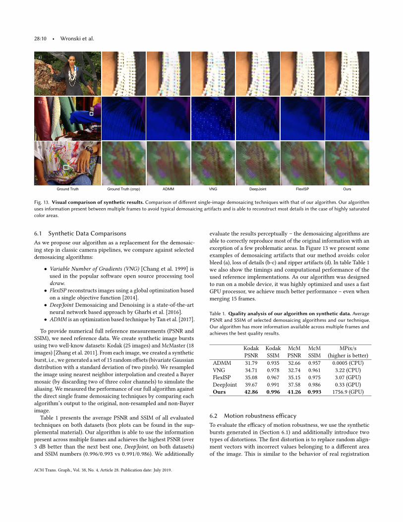
Fig. 13. Visual comparison of synthetic results. Comparison of different single-image demosaicing techniques with that of our algorithm. Our algorithm

uses information present between multiple frames to avoid typical demosaicing artifacts and is able to reconstruct most details in the case of highly saturated

color areas.

6.1 Synthetic Data Comparisons

As we propose our algorithm as a replacement for the demosaic-ing step in classic camera pipelines, we compare against selecteddemosaicing algorithms:

• Variable Number of Gradients (VNG) [Chang et al. 1999] isused in the popular software open source processing tooldcraw.

• FlexISP reconstructs images using a global optimization basedon a single objective function [2014].

• DeepJoint Demosaicing and Denoising is a state-of-the-artneural network based approach by Gharbi et al. [2016].

• ADMM is an optimization based technique by Tan et al. [2017].

To provide numerical full reference measurements (PSNR andSSIM), we need reference data. We create synthetic image burstsusing two well-know datasets: Kodak (25 images) and McMaster (18images) [Zhang et al. 2011]. From each image, we created a syntheticburst, i.e., we generated a set of 15 randomoffsets (bivariate Gaussiandistribution with a standard deviation of two pixels). We resampledthe image using nearest neighbor interpolation and created a Bayermosaic (by discarding two of three color channels) to simulate thealiasing. We measured the performance of our full algorithm againstthe direct single frame demosaicing techniques by comparing eachalgorithm’s output to the original, non-resampled and non-Bayerimage.Table 1 presents the average PSNR and SSIM of all evaluated

techniques on both datasets (box plots can be found in the sup-plemental material). Our algorithm is able to use the informationpresent across multiple frames and achieves the highest PSNR (over3 dB better than the next best one, DeepJoint, on both datasets)and SSIM numbers (0.996/0.993 vs 0.991/0.986). We additionally

evaluate the results perceptually ś the demosaicing algorithms areable to correctly reproduce most of the original information with anexception of a few problematic areas. In Figure 13 we present someexamples of demosaicing artifacts that our method avoids: colorbleed (a), loss of details (b-c) and zipper artifacts (d). In table Table 1we also show the timings and computational performance of theused reference implementations. As our algorithm was designedto run on a mobile device, it was highly optimized and uses a fastGPU processor, we achieve much better performance ś even whenmerging 15 frames.

Table 1. Quality analysis of our algorithm on synthetic data. Average

PSNR and SSIM of selected demosaicing algorithms and our technique.

Our algorithm has more information available across multiple frames and

achieves the best quality results.

Kodak Kodak McM McM MPix/sPSNR SSIM PSNR SSIM (higher is better)

ADMM 31.79 0.935 32.66 0.957 0.0005 (CPU)VNG 34.71 0.978 32.74 0.961 3.22 (CPU)FlexISP 35.08 0.967 35.15 0.975 3.07 (GPU)DeepJoint 39.67 0.991 37.58 0.986 0.33 (GPU)Ours 42.86 0.996 41.26 0.993 1756.9 (GPU)

6.2 Motion robustness efficacy

To evaluate the efficacy of motion robustness, we use the syntheticbursts generated in (Section 6.1) and additionally introduce twotypes of distortions. The first distortion is to replace random align-ment vectors with incorrect values belonging to a different areaof the image. This is similar to the behavior of real registration



Full picture One Frame+ DeepJoint

One Frame+ VNG

Hasinoff et al. [2016]+ DeepJoint OursHasinoff et al. [2016]

+ VNG

Fig. 14. Comparison with demosaicing techniques: Our method compared with dcraw’s Variable Number of Gradients [Chang et al. 1999] and Deep-

Joint [Gharbi et al. 2016]. Both demosaicing techniques are applied to either one frame from a burst or result of burst merging as described in Hasinoff

et al. [2016]. Readers are encouraged to zoom in aggressively (300% or more).

algorithms in case of significant movement and occlusion. We cor-rupt this way with an increasing percentage of local alignment tilesp = [10%, .., 50%].

The second type of distortion is to introduce random noise tothe alignment vectors, thereby shifting each image tile by a small,random amount. This type of distortion is often caused by the noiseor aliasing in the real images, or alignment ambiguity due to theaperture problem. We add such noise independently to each tileand use normally distributed noise with standard deviation σ =

[0.05, .., 0.25] displacement pixels.Examples of both evaluations can be seen in (Figure 17). Under

very strong distortion, the algorithm fuses far fewer frames andbehaves similarly to single-frame demosaicing algorithms. While itshows similar artifacts to the other demosaicing techniques (colorfringing, loss of detail), no multi-frame fusion artifact is present.In the supplemental material, we include the PSNR analysis of theerror with increasing amount of corruption, and more examples ofhow our motion robustness works on many different real burstscontaining complex local motion or scene changes.

6.3 Comparison on Real Captured Bursts

We perform comparisons on real raw bursts captured with a GooglePixel 3 phone camera. We compare against both single-frame demo-saicing and the spatio-temporal Wiener-filter described by Hasinoffet al. [2016], which also performs a burst merge. As the output of alltechniques is in linear space and is blurred by the lens, we sharpenit with an unsharp mask filter (with a standard deviation of threepixels) and apply global tonemapping ś an S-shaped curve withgamma correction. We present some examples of this comparisonin Figure 14. It shows that our algorithm produces the most detailedimages with the least amount of noise. Our results do not displayartifacts like zippers in case of VNG or structured pattern noise incase of DeepJoint. We show more examples in the supplementalmaterial.We also conducted a user study to evaluate the quality of our

method. For the study, we randomly generated four 250 × 250 pixelcrops from each of the images presented in Figure 14. To avoidcrops with no image content, we discarded crops where the standarddeviation of pixel intensity was measured to be less than 0.1. Inthe study, we examined all paired examples between our method



Full picture VNG+ FRVSR (blur=0.0)

DeepJoint+ FRVSR (blur=0.0)

VNG+ FRVSR (std=0.075)

Ours + Upscale 4x

DeepJoint+ FRVSR (std=0.075)

Fig. 15. Comparison with video super-resolution. Our method compared with FRVSR [Sajjadi et al. 2018] applied to bursts of images demosaiced with

VNG [Chang et al. 1999] or DeepJoint [Gharbi et al. 2016]. Readers are encouraged to zoom aggressively (300% or more).

Full picture Hasinoff et al. [2016] Ours Full picture Hasinoff et al. [2016] Ours

Fig. 16. End-to-end comparison as a replacement for the merge and demosaicing steps used in a camera pipeline. Six bursts captured with a

smartphone processed by a full camera pipeline described by Hasinoff et al. [2016]. Image crops on the left show results of merging using a temporal Wiener

filter together with demosaicing, while image crops on the right show results of our algorithm. Our results show higher image resolution with more visible

details and no aliasing effects.



Reference 20% Corrupted tiles 40% Corrupted tiles 40% corrupted tiles Robustness off

Reference Alignment noise 0.05 pixels Alignment noise 0.3 pixels Alignment noise 0.3 pixelsRobustness off

Fig. 17. Image quality degradation undermisalignment. Top row:Visual quality degradation caused by randomly corrupted andmisaligned tiles.Bottom

row: Visual quality degradation caused by noise added to the alignment vectors. From left to right we show the outputs corresponding to progressively

more corrupted input data. The far-right example shows how the algorithm would behave without the motion robustness component. We observe that

with increasing distortion rate, the algorithm tends to reject most frames, and results resemble a simple demosaicing algorithm with similar limitations and

artifacts, but does not show fusion artifacts.

Table 2. User study:We used Amazon Mechanical Turk and asked 115 people - ‘Which camera quality do you prefer?’. Shown, is a confusion matrix with

the participants’ nominated preference for each algorithm with respect to the other algorithms examined. Each entry is the fraction of cases where the row

method was preferred relative to the column method. Our algorithm (highlighted in bold) was found to be preferred in more that 79% of cases than that of the

next best competing algorithm (Hasinoff et al. + DeepJoint).

One Frame One Frame Hasinoff et al. Hasinoff et al.DeepJoint VNG + DeepJoint VNG Ours

One Frame + DeepJoint - 0.495 0.198 0.198 0.059One Frame + VNG 0.505 - 0.099 0.168 0.059Hasinoff et al. + DeepJoint 0.802 0.901 - 0.624 0.208Hasinoff et al. + VNG 0.802 0.832 0.376 - 0.099Ours 0.941 0.941 0.792 0.901 -

and the other compared methods. Using Amazon Mechanical Turkwe titled each pair of crops, Camera A and Camera B, and asked115 people to choose their prefered camera quality by asking thequestion - ‘Which camera quality do you prefer?’. The crops weredisplayed at 50% screen width and partipicants were limited to threeminutes to review each example pair (the average time spent was45 seconds). Table 2 shows the participants’ preferences for each ofthe compared methods. The results show that our method (in bold)is preferred in more than 79% of cases than that of the next bestmethod (Hasinoff et al. + DeepJoint).

As our algorithm is designed to be used inside a camera pipeline,we additionally evaluate the visual quality when our algorithm isused as a replacement of Wiener merge and demosaicing insidethe [Hasinoff et al. 2016] pipeline. Some examples and comparisonscan be seen in Figure 16.

Finally, we compared our approach with FRVSR [Sajjadi et al.2018], state-of-the-art deep learning based video super-resolution.We present some examples of this comparison in Figure 15 (addi-tional examples can be found in the supplemental material). Notethat our approach does not directly compete with this method sinceFRVSR: a. uses RGB images as the input (to be able to create thecomparison we apply VNG and DeepJoint to the input Bayer im-ages); b. produces upscaled images (4x the input resolution) makinga direct PSNR comparison difficult; c. requires separate training fordifferent light levels and amounts of noise present in the images.In consultation with the authors of FRVSR, we used two differentversions of their network to enable the fairest possible comparison.These different versions were not trained by us, but had been trainedearlier and reported in their paper. The versions of their network



2 4 6 8 10 12 14

Number of merged frames

30

35

40

45

PS

NR

(dB

)

Low SNR [0.0, 20.0)

Mid. SNR [20.0, 30.0)

High SNR (30.0, 40.0]

2 4 6 8 10 12 14

Number of merged frames

-16

-14

-12

-10

-8

-6

-4

-2

0

Diffe

rence in S

quare

dG

radie

nt M

agnitude o

f Y

Channel

10-6

Low SNR [0.0, 20.0)

Mid. SNR [20.0, 30.0)

High SNR (30.0, 40.0]

b)a)

Fig. 18. (a) PSNR results across different SNR ranges. The PSNR is measured

between the result of merging 15 frames to that of merging n frames where

n = [1, .., 14]. (b) Plot presenting the sharpness (measured as average

luminance gradient squared) difference between the result of merging 15

frames to that of merging n frames where n = [1, .., 14]. We observe

different behavior between low and high SNR of the base frame. In good

lighting conditions, sharpness reaches a peak around seven frames and then

starts to degrade slowly.

reported in our paper were the best performing for the given light-ing and noise conditions: one trained on noisy input images withnoise standard deviation of 0.075, the other on training data withoutany blur applied. We show our method (after upscaling 4x [Romanoet al. 2017]) compared with those two versions of FRVSR. In all cases,our method outperforms the combination of VNG and FRVSR. Ingood light, our method shows amounts of detail comparable to thecombination of DeepJoint and FRVSR at a fraction of their compu-tational costs (Section 6.5), while in low light, our method showsmore detailed images, no visual artifacts, and less noise.

6.4 Quality Dependence on the Number of Merged Frames

We use 586 bursts captured with a mobile camera across differentlighting to analyze the effect of merging different numbers of frames.Theoretically, with the increase in the number of frames we havemore information and observe better SNR. However, the registrationis imperfect, and the scene can change if the overall exposure timeis too long. Therefore, the inclusion of too many frames in the burstcan diminish the quality of the results (Figure 18 (b)).The algorithm’s current use of 15 merged frames was chosen

since it was found to produce high quality merged results fromlow-to-high SNR, and it was within the processing capabilities of asmartphone application. We show in Figure 18 (a) behavior of thePSNR as a function of n merged frames for n = [1, ..., 15] and acrossthree different SNR ranges. We observe approximately linear PSNRincrease due to frame noise variance reduction with the increasingnumber of frames. In case of good lighting conditions the impercep-tible error of PSNR 40 dB is achieved around eight frames, whilein low light the difference can be observed up to 15 frames. Thisbehavior is consistent with the perceptual evaluation presented inFigure 19.

Table 3. Computational performance analysis of our algorithm. We

analyze timing and memory usage for two different hardware platforms,

a mobile and a desktop GPU. Timing cost comprises a fixed cost part at

beginning and the end of the pipeline, while cost per frame grows linearly

with the number of merged frames. The cost scales linearly with the number

of pixels. Runtime computational and memory cost makes our algorithm

practical for use on a mobile device.

GPU Fixed cost Cost per frame Memory cost

Adreno 630 15.4 ms 7.8 ms / MPix 22 MB / MPixGTX 980 0.83 ms 0.4 ms / MPix 22 MB / MPix

6.5 Computational Performance

Our algorithm is implemented using OpenGL / OpenGL ES pixelshaders. We analyze the computational performance of our methodon both a Linux workstation with an nVidia GTX 980 GPU andon a mobile phone with a Qualcomm Adreno 630 GPU (includedin many high-end 2018 mobile phones, including Google Pixel 3).Performance and memory measurements to create a merged im-age can be found in Table 3. They are measured per output imagemegapixel and scale linearly with the pixel count. Because our algo-rithm merges the input images in an online fashion, the memoryconsumption is not dependent on the frame count. The fixed ini-tialization and finalizing cost is also not dependent on the framecount. Those numbers indicate that our algorithm is multiple ordersof magnitude faster than the neural network [Gharbi et al. 2016] oroptimization [Heide et al. 2014] based techniques.

Similarly, our method is approximately two orders of magnitudefaster as compared to FRVSR [Sajjadi et al. 2018] reported time of191ms to process a single Full HD image on an nVidia P100 (10.5MPix/s), even without taking into account the costs of demosaicingevery burst frame. Furthermore, the computational performance ofour algorithm is comparable to that reported by Hasinoff et al. [2016]ś 1200 ms for just their merge technique in low light conditions,excluding demosaicing.

7 DISCUSSION AND LIMITATIONS

In this section, we discuss some of the common limitations of multi-frame SR approaches due to hardware, noise, and motion require-ments. We then show how our algorithm performs in some of thecorner cases.

7.1 Device Optics and Sampling

By default our algorithm produces full RGB images at the resolutionof the raw burst, but we can take it further. The algorithm recon-structs a continuous representation of the image, which we canresample to the desired magnification and resolution enhancementfactors. The achievable super-resolution factor is limited by physicalfactors imposed by the camera design. The most important factor isthe sampling ratio 5 at the focal plane, or sensor array. In practicalterms, this means the lens must be sharp enough to produce a rela-tively small lens spot size compared to the pixel size. The samplingratio for the main cameras on leading mobile phones such as the

5Ratio of the diffraction spot size of the lens to the number of pixels in the spot. Asampling ratio of two and above avoids aliasing.



Full picture 4 frames 7 frames 10 frames 15 frames

Low

SN

R s

cene

Hig

h S

NR

sce

ne

Fig. 19. Visual differences caused by merging a different number of frames in the case of high (top) and low (bottom) SNR scenes. In the case the of high

SNR scenes, we do not observe any image quality increase when using more than seven frames. On the other hand, in the case of low light scenes with worse

SNR, we can observe a quality increase and better denoising.

3.0x2.0x1.5x1.0x

Fig. 20. Different target grid resolutions. Two different crops from a photo of a test chart, from left to right 1×, 1.5×, 2×, and 3×. Results were upscaled

using a 3-lobe Lanczos filter to the same size. The combination of our algorithm and the phone’s optical system with sampling ratio of 1.5 leads to significantly

improved results at 1.5× zoom, small improvement up to 2× zoom (readers are encouraged to zoom in) and no additional resolution gains returns thereafter.

Apple iPhone X and the Google Pixel 3 are in the range 1.5 to 1.8 (inthe luminance channel) which are lower than the critical samplingratio of two. Since the sensor is color-filtered, the result Bayer rawimages are aliased more ś the green channel is 50% more aliased,where as the blue and red ones can be as much as twice more aliased.

We analyze super-resolution limits of our algorithm used on asmartphone using a raw burst captured with a Google Pixel 3 cam-era with a sampling ratio of approximately 1.5. We use differentmagnification factors ranging from 1× (just replacing the demosaic-ing step) up to 3× and use a handheld photo of a standard test chart.Figure 20 presents a visual comparison between results achievedby running our algorithm on progressively larger target grid reso-lutions. The combination of our algorithm and the phone’s opticalsystem leads to significantly improved results at 1.5× zoom, small

improvement up to 2× zoom and no additional resolution gainsreturns thereafter. Those results suggest that our algorithm is ableto deliver resolution comparable to a dedicated tele lenses at modestmagnification factors (under 2×).

7.2 Noise-dependent Tuning

Beyond the optical/sensor design, there are also fundamental limitsto super-resolution in the presence of noise. This idea has beenstudied in a number of publications from both theoretical and ex-perimental standpoints [Helstrom 1969; Lu et al. 2018; Shahram andMilanfar 2006]. These works all note a power law relationship be-tween achievable resolution and (linear) SNR. Namely, the statisticallikelihood of resolving two nearby point sources is proportional toSNRp , where 0 < p < 1 depends on the imaging system. As SNR



Fig. 21. Comparison of behavior in low light. Left: Single frame demo-

saiced and denoised with a spatial denoiser.Middle:Wiener filter spatio-

temporal denoising of a burst [Hasinoff et al. 2016] followed by demosaicing.

Right: Spatio-temporal denoising of our merge algorithm while preserving

sharp local image details.

Fig. 22. Occlusion and local motion in low light: Left: Our motion ro-

bustness logic causes some regions to merge only single frame due to occlu-

sions or misalignments. In low light it causes more noise in those regions.

Right: Additional spatial denoising with strength inversely proportional to

the merged frame count fixes those problems.

Fig. 23. Fusion artifacts: Left: Aperture problem can create shifted object

edges. Right: High frequency regions with subpixel motion can contribute

to distinctive high frequency artifacts.

tends to zero, the ability to resolve additional details will also tendto zero rapidly. Therefore, at low light levels, the ability to super-resolve is reduced, and most of the benefits of our algorithm will bemanifested as spatio-temporal denoising that preserves the imagedetails (Figure 21). Due to the difference between low and goodlight levels and the trade-offs it enforces (e.g., resolution enhance-ment vs. stronger noise reduction), we depend on the base framesignal-to-noise ratio for selecting the kernel tuning parameters. Theestimated SNR is the only input parameter to our tuning and is com-puted based on the average image brightness and the noise modelSection 5.2.2. When presenting all of the visual results in this text,we have not manually adjusted any of the parameters per image and

instead utilized this automatic SNR-dependent parameter selectiontechnique. The locally adaptive spatio-temporal denoising of ouralgorithm motivated its use as a part of the Night Sight mode onGoogle’s Pixel 3 smartphone.

7.3 Lack of Movement

As we highlighted in the main text, a key aspect of our approach isthe reliance on random, natural tremor that is ubiquitously presentin hand-held photography. When the device is immobilized (forexample when used on a tripod), we can introduce additional move-ment using active, moving camera components. Namely, if the gy-roscope on the device detects no motion, the sensor or the OpticalImage Stabilization system can be moved in a controlled pattern.This approach has been successfully used in practice using sensorshifts (Sony A6000, Pentax FF K1, Olympus OM-D E-M1 or PanasonicLumix DC-G9) or the OIS movement [Wronski and Milanfar 2018].

7.4 Excessive Local Movement and Occlusion

Our motion robustness calculation (Section 5.2) excludes misaligned,moving or occluded regions from fusion to prevent visual artifacts.However, in cases of severe local movement or occlusion, a regionmight get contributions only from the base frame, and our algo-rithm produces results resembling single frame demosaicing withsignificantly lower quality (Section 6.2). In low light condition, theseregions would also be much noiser than others, but additional local-ized spatial denoising can improve the quality, as demonstrated inFigure 22.

7.5 Fusion Artifacts

The proposed robustness logic (Section 5.2) can still allow for spe-cific minor fusion artifacts. The alignment aperture problem cancause some regions to be wrongly aligned with similarly lookingregions in a different part of the image. If the difference is onlysubpixel, our algorithm could incorrectly merge those regions (Fig-ure 23 left). This limitation could be improved by using a betteralignment algorithm or a dedicated detector (we present one in thesupplemental material).Additionally, burst images may contain small, high frequency

scene changes ś for example caused by ripples on the water orsmall magnitude leaf movement (Figure 23 right). When those re-gions get correctly aligned, the similarity between the frames makesour algorithm occasionally not able to distinguish those changesfrom real subpixel details and fuses them together. Those problemshave a characteristic visual structure and could be addressed by aspecialized artifact detection and correction algorithm.

8 CONCLUSIONS AND FUTURE WORK

In this paper we have presented a super-resolution algorithm thatworks on bursts of raw, color-filtered images. We have demon-strated that given random, natural hand tremor, reliable imagesuper-resolution is indeed possible and practical. Our approachhas low computational complexity that allows for processing at in-teractive rates on a mass-produced mobile device. It does not requirespecial equipment and can work with a variable number of inputframes.



Our approach extends existing non-parametric kernel regres-sion to merge Bayer raw images directly onto a full RGB frame,bypassing single-frame demosaicing altogether. We have demon-strated (on both synthetic and real data) that the proposed methodachieves better image quality than (a) state of the art demosaicingalgorithms, and (b) state of the art burst processing pipelines thatfirst merge raw frames and then demosaic (e.g. Hasinoff et al. [2016]).By reconstructing the continuous signal, we are able to resampleit onto a higher resolution discrete grid and reconstruct the imagedetails of higher resolution than the input raw frames. With locallyadaptive kernel parametrization, and a robustness model, we can si-multaneously enhance resolution and achieve local spatio-temporaldenoising, making the approach suitable for capturing scenes invarious lighting conditions, and containing complex motion.

An avenue of future research is extending ourwork to video super-resolution, producing a sequence of images directly from a sequenceof Bayer images. While our unmodified algorithm could producesuch sequence by changing the anchor frame and re-running itmultiple times, this would be inefficient and result in redundantcomputations.For other future work, we note that computational photogra-

phy, of which this paper is an example, has gradually changed thenature of photographic image processing pipelines. In particular,algorithms are no longer limited to pixel-in / pixel-out arithmeticwith only fixed local access patterns to neighboring pixels. Thischange suggests that new approaches may be needed for hardwareacceleration of image processing.Finally, depending on handshake to place red, green, and blue

samples below each pixel site suggest that perhaps the design ofcolor filter arrays should be reconsidered; perhaps the classic RGGBBayer mosaic is no longer optimal. Perhaps the second G pixel canbe replaced with another sensing modality. More exotic CFAs havetraditionally suffered from reconstruction artifacts, but our ratherdifferent approach to reconstruction might mitigate some of theseartifacts.

ACKNOWLEDGMENTS

We gratefully acknowledge current and former colleagues fromcollaborating teams across Google including: Haomiao Jiang, JiawenChen, Yael Pritch, James Chen, Sung-Fang Tsai, Daniel Vlasic, PascalGetreuer, Dillon Sharlet, Ce Liu, Bill Freeman, Lun-Cheng Chu,Michael Milne, and Andrew Radin. Integration of our algorithmwith the Google Camera App as Super-Res Zoom and Night Sight

mode was facilitated with generous help from the Android camerateam.We also thank the anonymous reviewers for valuable feedbackthat has improved our manuscript.

REFERENCESAdobe. 2012. Digital Negative (DNG) Specification. https://www.adobe.com/content/

dam/acom/en/products/photoshop/pdfs/dng_spec_1.4.0.0.pdf.Simon Baker and Takeo Kanade. 2002. Limits on super-resolution and how to break

them. IEEE Trans. PAMI 24, 9 (2002), 1167ś1183.Bryce E Bayer. 1976. Color imaging array. US Patent 3,971,065.Stefanos P Belekos, Nikolaos P Galatsanos, and Aggelos K Katsaggelos. 2010. Maximum

a posteriori video super-resolution using a new multichannel image prior. IEEETrans. Image Processing 19, 6 (2010), 1451ś1464.

Moshe Ben-Ezra, Assaf Zomet, and Shree K Nayar. 2005. Video super-resolution usingcontrolled subpixel detector shifts. IEEE Trans. PAMI 27, 6 (2005), 977ś987.

Josef Bigün, Goesta H. Granlund, and Johan Wiklund. 1991. Multidimensional orienta-tion estimation with applications to texture analysis and optical flow. IEEE Trans.PAMI 8 (1991), 775ś790.

James F Blinn. 1982. A generalization of algebraic surface drawing. ACM TOG 1, 3(1982), 235ś256.

Edward Chang, Shiufun Cheung, and Davis Y Pan. 1999. Color filter array recoveryusing a threshold-based variable number of gradients. In Sensors, Cameras, andApplications for Digital Photography, Vol. 3650. 36ś44.

CIPA. 2018. CIPA Report. www.cipa.jp/stats/report_e.html. [Online; accessed 29-Nov-2018].

Sabrina Dammertz and Alexander Keller. 2008. Image synthesis by rank-1 lattices. InMonte Carlo and Quasi-Monte Carlo Methods 2006. 217ś236.

Michael Drobot. 2014. Hybrid reconstruction anti-aliasing. In ACM SIGGRAPH Courses.Joan Duran and Antoni Buades. 2014. Self-similarity and spectral correlation adaptive

algorithm for color demosaicking. IEEE Trans. Image Processing 23, 9 (2014), 4031ś4040.

Michael Elad and Arie Feuer. 1997. Restoration of a single superresolution image fromseveral blurred, noisy, and undersampled measured images. IEEE Trans. ImageProcessing 6, 12 (1997), 1646ś1658.

Sina Farsiu, Michael Elad, and Peyman Milanfar. 2006. Multiframe demosaicing andsuper-resolution of color images. IEEE Trans. Image Processing 15, 1 (2006), 141ś159.

David J Fleet and Allan D Jepson. 1990. Computation of component image velocityfrom local phase information. IJCV 5, 1 (1990), 77ś104.

Flickr. 2017. Top Devices of 2017 on Flickr. https://blog.flickr.net/en/2017/12/07/top-devices-of-2017/. [Online; accessed 11-Jan-2019].

Alessandro Foi, Mejdi Trimeche, Vladimir Katkovnik, and Karen Egiazarian. 2008.Practical Poissonian-Gaussian noise modeling and fitting for single-image raw-data.IEEE Trans. Image Processing 17, 10 (2008), 1737ś1754.

Michaël Gharbi, Gaurav Chaurasia, Sylvain Paris, and Frédo Durand. 2016. Deep jointdemosaicking and denoising. ACM TOG 35, 6 (2016), 191.

Clément Godard, Kevin Matzen, and Matt Uyttendaele. 2018. Deep burst denoising. InProc. ECCV, Vol. 11219. 560ś577.

Tomomasa Gotoh and Masatoshi Okutomi. 2004. Direct super-resolution and registra-tion using raw CFA images. In Proc. CVPR, Vol. 2.

Chris Harris and Mike Stephens. 1988. A combined corner and edge detector.. In AlveyVision Conference, Vol. 15. 10ś5244.

Samuel W Hasinoff, Dillon Sharlet, Ryan Geiss, Andrew Adams, Jonathan T Barron,Florian Kainz, Jiawen Chen, and Marc Levoy. 2016. Burst photography for highdynamic range and low-light imaging on mobile cameras. ACM TOG 35, 6 (2016),192.

Sung Hee Park and Marc Levoy. 2014. Gyro-based multi-image deconvolution forremoving handshake blur. In Proc. ICCV. 3366ś3373.

Felix Heide, Markus Steinberger, Yun-Ta Tsai, Mushfiqur Rouf, Dawid Pajkk, DikpalReddy, Orazio Gallo, Jing Liu, Wolfgang Heidrich, et al. 2014. FlexISP: A flexiblecamera image processing framework. ACM TOG 33, 6 (2014), 231.

Carl WHelstrom. 1969. Detection and resolution of incoherent objects by a background-limited optical system. JOSA 59, 2 (1969), 164ś175.

Robert Herzog, Elmar Eisemann, Karol Myszkowski, and H-P Seidel. 2010. Spatio-temporal upsampling on the GPU. In Proceedings of the 2010 ACM SIGGRAPH sym-posium on Interactive 3D Graphics and Games. 91ś98.

Keigo Hirakawa and Thomas W Parks. 2005. Adaptive homogeneity-directed demo-saicing algorithm. IEEE Trans. Image Processing 14, 3 (2005), 360ś369.

Keigo Hirakawa and Thomas W Parks. 2006. Joint demosaicing and denoising. IEEETrans. Image Processing 15, 8 (2006), 2146ś2157.

Terence D Hunt. 2004. Image Super-Resolution Using Adaptive 2-D Gaussian BasisFunction Interpolation. Technical Report. Air Force Inst of Tech Wright-PattersonAFB OH School of Engineering.

Michal Irani and Shmuel Peleg. 1991. Improving resolution by image registration.CVGIP: Graphical models and image processing 53, 3 (1991), 231ś239.

Jorge Jimenez, Diego Gutierrez, Jason Yang, Alexander Reshetov, Pete Demoreuille,Tobias Berghoff, Cedric Perthuis, Henry Yu, MorganMcGuire, Timothy Lottes, HughMalan, Emil Persson, Dmitry Andreev, and Tiago Sousa. 2011. Filtering Approachesfor Real-Time Anti-Aliasing. In ACM SIGGRAPH Courses.

Takeo Kanade and Masatoshi Okutomi. 1991. A stereo matching algorithm with anadaptive window: Theory and experiment. In Proc. IEEE ICRA. IEEE, 1088ś1095.

Brian Karis. 2014. High-Quality Temporal Supersampling. In ACM SIGGRAPH Courses.Darwin T Kuan, Alexander A Sawchuk, Timothy C Strand, and Pierre Chavel. 1985.

Adaptive noise smoothing filter for images with signal-dependent noise. IEEE Trans.PAMI 2 (1985), 165ś177.

Yeon Ju Lee and Jungho Yoon. 2010. Nonlinear image upsampling method basedon radial basis function interpolation. IEEE Trans. Image Processing 19, 10 (2010),2682ś2692.

Brian Leung, Gwanggil Jeon, and Eric Dubois. 2011. Least-squares lumaśchromademultiplexing algorithm for Bayer demosaicking. IEEE Trans. Image Processing 20,7 (2011), 1885ś1894.


https://www.adobe.com/content/dam/acom/en/products/photoshop/pdfs/dng_spec_1.4.0.0.pdf

https://www.adobe.com/content/dam/acom/en/products/photoshop/pdfs/dng_spec_1.4.0.0.pdf

www.cipa.jp/stats/report_e.html

https://blog.flickr.net/en/2017/12/07/top-devices-of-2017/

https://blog.flickr.net/en/2017/12/07/top-devices-of-2017/


Tzu-Mao Li, Michaël Gharbi, Andrew Adams, Frédo Durand, and Jonathan Ragan-Kelley. 2018. Differentiable programming for image processing and deep learningin Halide. ACM Trans. Graph. (Proc. SIGGRAPH) 37, 4 (2018), 139:1ś139:13.

Xin Li, Bahadir Gunturk, and Lei Zhang. 2008. Image demosaicing: A systematic survey.In Visual Communications and Image Processing 2008, Vol. 6822. 68221J.

Ce Liu and Deqing Sun. 2011. A Bayesian approach to adaptive video super resolution.In Proc. CVPR. IEEE, 209ś216.

Xiao-Ming Lu, Hari Krovi, Ranjith Nair, Saikat Guha, and Jeffrey H Shapiro. 2018.Quantum-optimal detection of one-versus-two incoherent optical sources witharbitrary separation. arXiv preprint arXiv:1802.02300 (2018).

Bruce D Lucas and Takeo Kanade. 1981. An iterative image registration technique withan application to stereo vision. (1981).

Rastislav Lukac and Konstantinos N Plataniotis. 2004. Normalized color-ratio modelingfor CFA interpolation. IEEE Trans. Consumer Electronics 50, 2 (2004), 737ś745.

Hugh Malan. 2012. Real-Time Global Illumination and Reflections in Dust 514. In ACMSIGGRAPH Courses.

John Marshall and E Geoffrey Walsh. 1956. Physiological tremor. Journal of neurology,neurosurgery, and psychiatry 19, 4 (1956), 260.

Ben Mildenhall, Jonathan T Barron, Jiawen Chen, Dillon Sharlet, Ren Ng, and RobertCarroll. 2018. Burst denoising with kernel prediction networks. In Proc. CVPR.2502ś2510.

Yusuke Monno, Daisuke Kiku, Masayuki Tanaka, and Masatoshi Okutomi. 2015. Adap-tive residual interpolation for color image demosaicking. In Proc. IEEE ICIP. 3861ś3865.

Matthias Müller, Barbara Solenthaler, Richard Keiser, and Markus Gross. 2005. Particle-based fluid-fluid interaction. In Proceedings of the 2005 ACM SIGGRAPH/Eurographicssymposium on Computer animation. 237ś244.

NIH. 2018. Tremor Fact. www.ninds.nih.gov/Disorders/Patient-Caregiver-Education/Fact-Sheets/Tremor-Fact-Sheet. [Online; accessed 29-Nov-2018].

Harry Nyquist. 1928. Certain topics in telegraph transmission theory. Transactions ofthe American Institute of Electrical Engineers 47, 2 (1928), 617ś644.

Athanasios Papoulis. 1977. Generalized sampling expansion. IEEE Trans. Circuits andSystems 24, 11 (1977), 652ś654.

Cameron N Riviere, R Scott Rader, and Nitish V Thakor. 1998. Adaptive cancelling ofphysiological tremor for improved precision in microsurgery. IEEE Trans. BiomedicalEngineering 45, 7 (1998), 839ś846.

Dirk Robinson and Peyman Milanfar. 2004. Fundamental performance limits in imageregistration. IEEE Trans. Image Processing 13, 9 (2004), 1185ś1199.

Dirk Robinson and Peyman Milanfar. 2006. Statistical performance analysis of super-resolution. IEEE Trans. Image Processing 15, 6 (2006), 1413ś1428.

Yaniv Romano, John Isidoro, and Peyman Milanfar. 2017. RAISR: Rapid and accurateimage super resolution. IEEE Trans. Computational Imaging 3, 1 (2017), 110ś125.

Mehdi S. M. Sajjadi, Raviteja Vemulapalli, and Matthew Brown. 2018. Frame-recurrentvideo super-resolution. In Proc. CVPR. 6626ś6634.

Marco Salvi. 2016. An excursion in temporal super sampling. GDC2016 From the LabBench: Real-Time Rendering Advances from NVIDIA Research (2016).

E. A. Schäfer. 1886. On the rhythm of muscular response to volitional impulses in man.The Journal of Physiology 7, 2 (1886), 111ś117.

Morteza Shahram and Peyman Milanfar. 2006. Statistical and information-theoreticanalysis of resolution in imaging. IEEE Trans. Information Theory 52, 8 (2006),3411ś3437.

Masao Shimiziu and Masatoshi Okutomi. 2005. Sub-pixel estimation error cancellationon area-based matching. IJCV 63 (2005), 207ś224. Issue 3.

Tiago Sousa. 2013. Graphics Gems CryENGINE3. In ACM SIGGRAPH Courses.Molly M Sturman, David E Vaillancourt, and Daniel M Corcos. 2005. Effects of aging

on the regularity of physiological tremor. Journal of Neurophysiology 93, 6 (2005),3064ś3074.

H Takeda, S Farsiu, and P Milanfar. 2006. Robust kernel regression for restoration andreconstruction of images from sparse noisy data. Proc. IEEE ICIP (2006), 1257ś1260.

H Takeda, S Farsiu, and P Milanfar. 2007. Kernel regression for image processing andreconstruction. IEEE Trans. Image Processing 16, 2 (2007), 349.

Hanlin Tan, Xiangrong Zeng, Shiming Lai, Yu Liu, and Maojun Zhang. 2017. Jointdemosaicing and denoising of noisy bayer images with ADMM. In Proc. IEEE ICIP.2951ś2955.

R.Y. Tsai and T.S. Huang. 1984. Multiframe image restoration and registration. AdvanceComputer Visual and Image Processing 1 (1984), 317ś339.

Patrick Vandewalle, Karim Krichane, David Alleysson, and Sabine Süsstrunk. 2007.Joint demosaicing and super-resolution imaging from a set of unregistered aliasedimages. In Digital Photography III, Vol. 6502. International Society for Optics andPhotonics, 65020A.

Neal Wadhwa, Rahul Garg, David E Jacobs, Bryan E Feldman, Nori Kanazawa, RobertCarroll, Yair Movshovitz-Attias, Jonathan T Barron, Yael Pritch, and Marc Levoy.2018. Synthetic depth-of-field with a single-camera mobile phone. ACM TOG 37, 4(2018), 64.

Hermann Weyl. 1910. Über die Gibbs’sche Erscheinung und verwandte Konvergen-zphänomene. Rendiconti del Circolo Matematico di Palermo (1884-1940) 30, 1 (01 Dec

1910), 377ś407.Bartlomiej Wronski and Peyman Milanfar. 2018. See Better and Further with Super

Res Zoom on the Pixel 3. https://ai.googleblog.com/2018/10/see-better-and-further-with-super-res.html.

Xiaolin Wu and Lei Zhang. 2006. Temporal color video demosaicking via motionestimation and data fusion. IEEE Trans. Circuits and Systems for Video Technology16 (2006). Issue 2.

J Yen. 1956. On nonuniform sampling of bandwidth-limited signals. IRE Trans. CircuitTheory 3, 4 (1956), 251ś257.

Jihun Yu and Greg Turk. 2013. Reconstructing surfaces of particle-based fluids usinganisotropic kernels. ACM TOG 32, 1 (2013), 5.

Lei Zhang, Xiaolin Wu, Antoni Buades, and Xin Li. 2011. Color demosaicking by localdirectional interpolation and nonlocal adaptive thresholding. Journal of Electronicimaging 20, 2 (2011), 023016.


www.ninds.nih.gov/Disorders/Patient-Caregiver-Education/Fact-Sheets/Tremor-Fact-Sheet

www.ninds.nih.gov/Disorders/Patient-Caregiver-Education/Fact-Sheets/Tremor-Fact-Sheet

https://ai.googleblog.com/2018/10/see-better-and-further-with-super-res.html

https://ai.googleblog.com/2018/10/see-better-and-further-with-super-res.html

handheld multi-frame super-resolution · 2019-08-23 · handheld multi-frame super-resolution •...

Documents