Champaign

Cliff Hastings Kelvin Mischo Michael Morrison

MATHEMATICA®

and Programming with the Wolfram Language™

HANDS-ON START TO WOLFRAM

SECOND EDITION

����� �� ��������

Introduction vii

���� � THE COMPLETE OVERVIEW 1

Chapter 1 The Very Basics 3Chapter 2 A Sample Project in Mathematica 11Chapter 3 Input and Output 21Chapter 4 Word Processing and Typesetting 43Chapter 5 Presenting with Slide Shows 59Chapter 6 Fundamentals of the Wolfram Language 73Chapter 7 Creating Interactive Models with a Single Command 93Chapter 8 Sharing Mathematica Notebooks 115Chapter 9 Finding Help 125

���� �� EXTENDING KNOWLEDGE 133

Chapter 10 2D and 3D Graphics 135Chapter 11 Visualizing Data 157Chapter 12 Styling and Customizing Graphics 179Chapter 13 Creating Figures and Diagrams with Graphics Primitives 213Chapter 14 Algebraic Manipulation and Equation Solving 233Chapter 15 Calculus 245Chapter 16 Differential Equations 261Chapter 17 Linear Algebra 271Chapter 18 Probability and Statistics 289Chapter 19 Importing and Exporting Data 305Chapter 20 Data Filtering and Manipulation 327Chapter 21 Working with Curated Data 359Chapter 22 Using Wolfram|Alpha Data in Mathematica 393Chapter 23 Statistical Functionality for Data Analysis 419Chapter 24 Creating Programs 437Chapter 25 Creating Parallel and GPU Programs 459

Index 477

CHAPTER 7Creating Interactive Models with aSingle Command

IntroductionOne of the most exciting features of Mathematica is the ability to create interactive modelswith a single command calledManipulate. The core idea ofManipulate is very simple: wrapit around an existing expression and introduce some parameters; Mathematica does the restin terms of creating a useful interface for exploring what happens when those parameters aremanipulated. This single command is a powerful tool for learning and teaching aboutphenomena and for creating models and simulations to support research activities.

Building a First ModelA common workflow is to start with something static, such as a plot, and then to make itinteractive usingManipulate. Take the following plot as an example, which plots sin(x)from 0 to 2 π.

Plot[Sin[x], {x, 0, 2π}]

� � � � � �

-���

-���

���

���

The goal may be to compare the curve of sin(x) with the curve of sin(2 x), the curve ofsin(3 x) and so on. In other words, to examine the behavior of sin( f x) when f is variedamong a large quantity of numbers.Manipulate provides an easy way to perform thisinvestigation by constructing an interactive model to explore this behavior.

��

To begin, it is important to know that usingManipulate requires three components:

1. Manipulate command2. Expression to manipulate by changing certain parameters3. Parameter specifications

An easy way to keep track of these components is to write commands involvingManipulateas follows.

Manipulate[expression to manipulate,parameter specifications]

This approach keeps each component on a separate line and provides an easy way to keeptrack of each separate component.

For the example introduced above, theManipulate command might be as follows.

Manipulate[Plot[Sin[frequency*x], {x, 0, 2π}],{frequency, 1, 5}]

���������

� � � � � �

-���

-���

���

���

The result is an interactive model with a slider bar that can be clicked and dragged tointeractively explore what happens as the value of frequency is changed. This specificmodel can be quite useful for explaining concepts of periodicity and frequency and wasbuilt from a single line of code—pretty impressive, and a representative example of thepower ofManipulate.

������� �

��

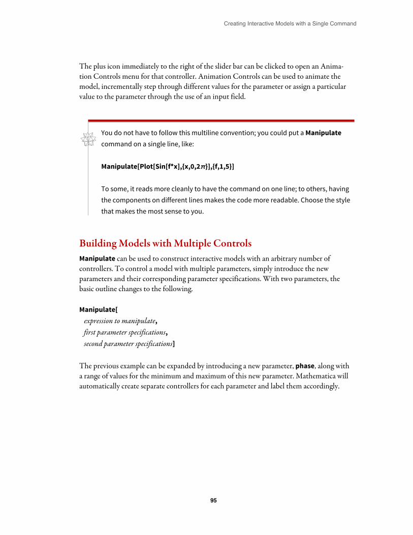
The plus icon immediately to the right of the slider bar can be clicked to open an Anima-tion Controls menu for that controller. Animation Controls can be used to animate themodel, incrementally step through different values for the parameter or assign a particularvalue to the parameter through the use of an input field.

� You do not have to follow this multiline convention; you could put aManipulatecommand on a single line, like:

Manipulate[Plot[Sin[f*x],{x,0,2π}],{f,1,5}]

To some, it reads more cleanly to have the command on one line; to others, havingthe components on different lines makes the code more readable. Choose the stylethat makes the most sense to you.

BuildingModels withMultiple ControlsManipulate can be used to construct interactive models with an arbitrary number ofcontrollers. To control a model with multiple parameters, simply introduce the newparameters and their corresponding parameter specifications. With two parameters, thebasic outline changes to the following.

Manipulate[expression to manipulate,first parameter specifications,second parameter specifications]

The previous example can be expanded by introducing a new parameter, phase, along witha range of values for the minimum and maximum of this new parameter. Mathematica willautomatically create separate controllers for each parameter and label them accordingly.

�������� ����������� ������ ���� � ������ �������

��

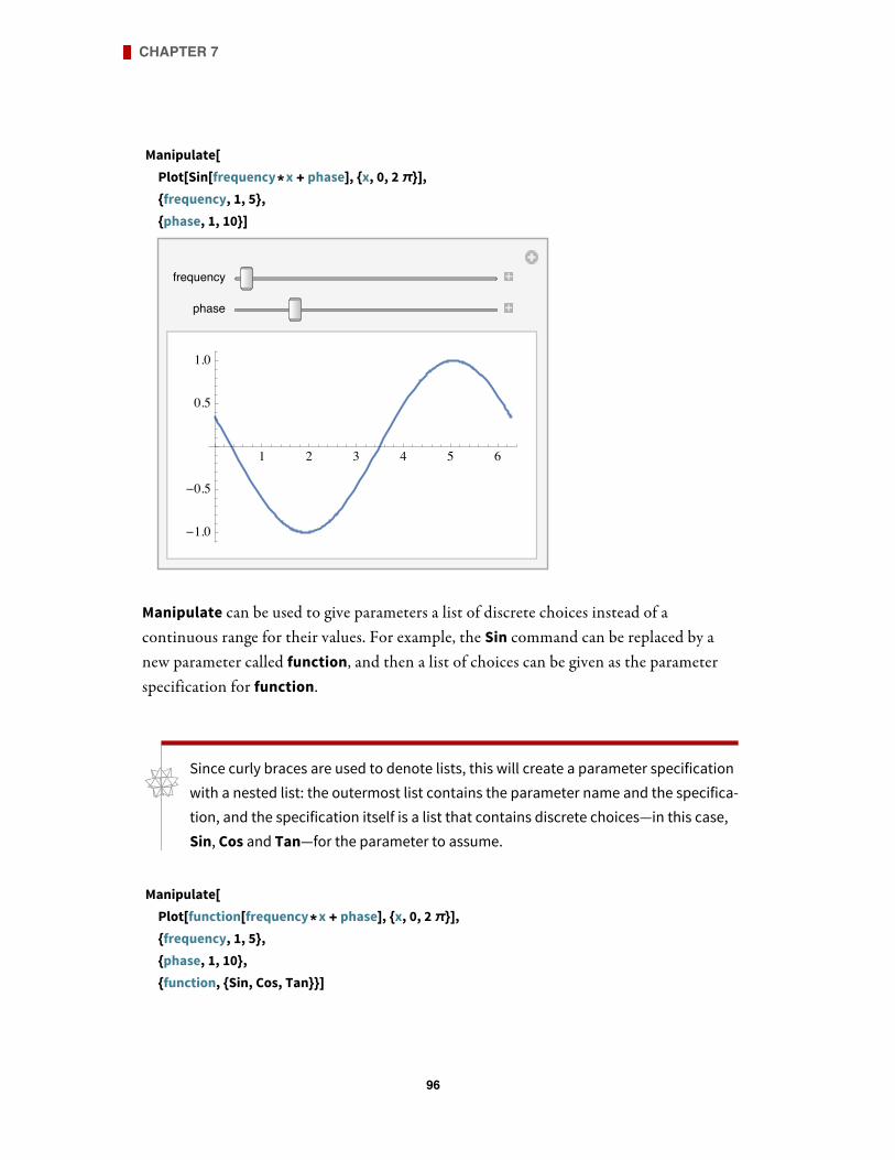
Manipulate[Plot[Sin[frequency*x + phase], {x, 0, 2π}],{frequency, 1, 5},{phase, 1, 10}]

���������

�����

� � � � � �

-���

-���

���

���

Manipulate can be used to give parameters a list of discrete choices instead of acontinuous range for their values. For example, the Sin command can be replaced by anew parameter called function, and then a list of choices can be given as the parameterspecification for function.

� Since curly braces are used to denote lists, this will create a parameter specificationwith a nested list: the outermost list contains the parameter name and the specifica-tion, and the specification itself is a list that contains discrete choices—in this case,Sin, Cos and Tan—for the parameter to assume.

Manipulate[Plot[function[frequency*x + phase], {x, 0, 2π}],{frequency, 1, 5},{phase, 1, 10},{function, {Sin, Cos, Tan}}]

������� �

��

���������

�����

�������� ��� ��� ���

� � � � � �

-���

-���

���

���

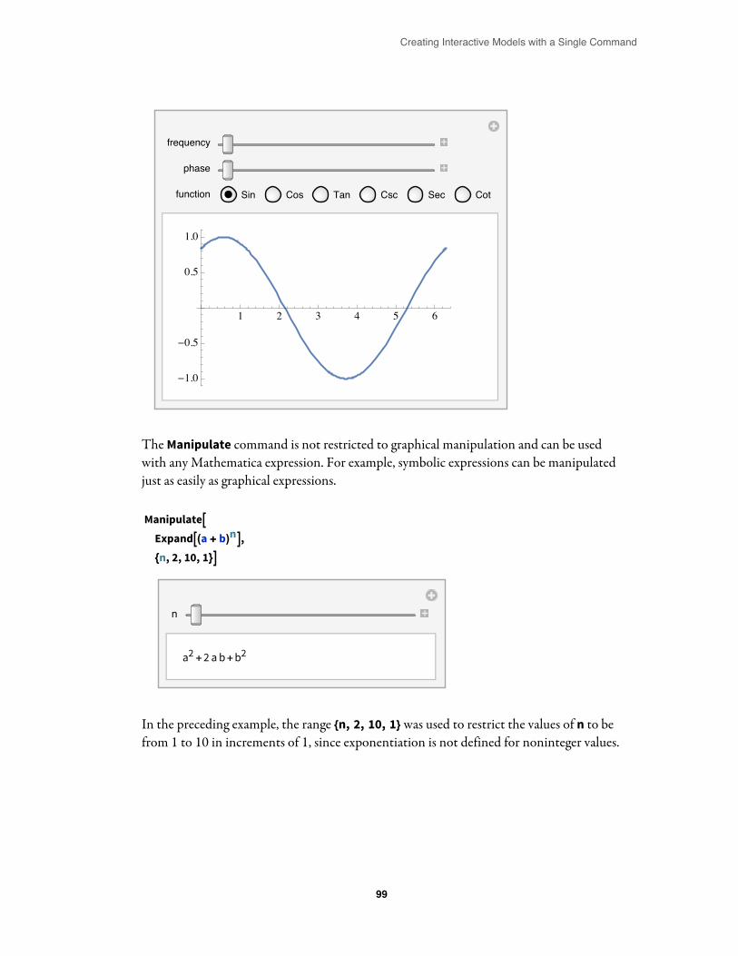
Mathematica has built-in heuristics to select appropriate controller types based onthe parameter specifications that have been given. For example, giving a long list ofchoices causes Manipulate to display the controller as a drop-down menu instead ofa list of buttons.

Manipulate[Plot[function[frequency*x + phase], {x, 0, 2π}],{frequency, 1, 5},{phase, 1, 10},{function, {Sin, Cos, Tan, Csc, Sec, Cot}}]

�������� ����������� ������ ���� � ������ �������

��

���������

�����

�������� ���

� � � � � �

-���

-���

���

���

� Like most everything in Mathematica, the output from commands can be cus-tomized through the use of options. If you want to force Mathematica to use aparticular control type, the ControlType option can be used with values such asSetter, Slider and RadioButtonBar. For example, if you add ControlType→RadioButtonBar between the two closing curly braces in the last parameterspecification in the preceding example, Mathematica will create a row of radiobuttons to set the value of function instead of giving you a drop-downmenu.

Manipulate[Plot[function[frequency*x + phase], {x, 0, 2π}],{frequency, 1, 5},{phase, 1, 10},{function, {Sin, Cos, Tan, Csc, Sec, Cot}, ControlType→ RadioButtonBar}]

������� �

��

���������

�����

�������� ��� ��� ��� ��� ��� ���

� � � � � �

-���

-���

���

���

TheManipulate command is not restricted to graphical manipulation and can be usedwith anyMathematica expression. For example, symbolic expressions can be manipulatedjust as easily as graphical expressions.

ManipulateExpand (a + b)n ,{n, 2, 10, 1}

�

a2+2 a b+b2

In the preceding example, the range {n, 2, 10, 1} was used to restrict the values of n to befrom 1 to 10 in increments of 1, since exponentiation is not defined for noninteger values.

�������� ����������� ������ ���� � ������ �������

��

Some Tips for Creating Useful Models

� The default results returned byManipulate are generally very useful and do notrequire any special customization. However, there are a few important points to beaware of, so we will discuss them here in order to help you avoid potential problems.

The Importance of PlotRange

The default behavior of commands like Plot is to automatically choose an appropriateviewing window unless a specific range is given. This means that whenManipulate is usedto change the value of a parameter, which has a resulting effect of changing the appearanceof a plot, the plot will immediately be redrawn with a new viewing window. The end resultis that manipulating a parameter may appear to change the axes for the plot rather than theplot itself.

The following screen shot shows an example of this behavior. On the left, the value of theparameter a is set to 3, and the plot axes are automatically chosen to fully display the behav-ior of the plot. On the right, the value of a is set to 6, and the plot is drawn accordingly.

This behavior can be avoided by specifying an explicit range to plot over. This can beaccomplished by using the PlotRange option for the Plot command, which forces the plotto be drawn with the specific plot range the user provides. PlotRange takes a list as itsargument (remember: lists are enclosed by curly braces), where the first element of the listis the minimum value for the plot range, and the second element of the list is the maximumvalue for the plot range.

������� �

���

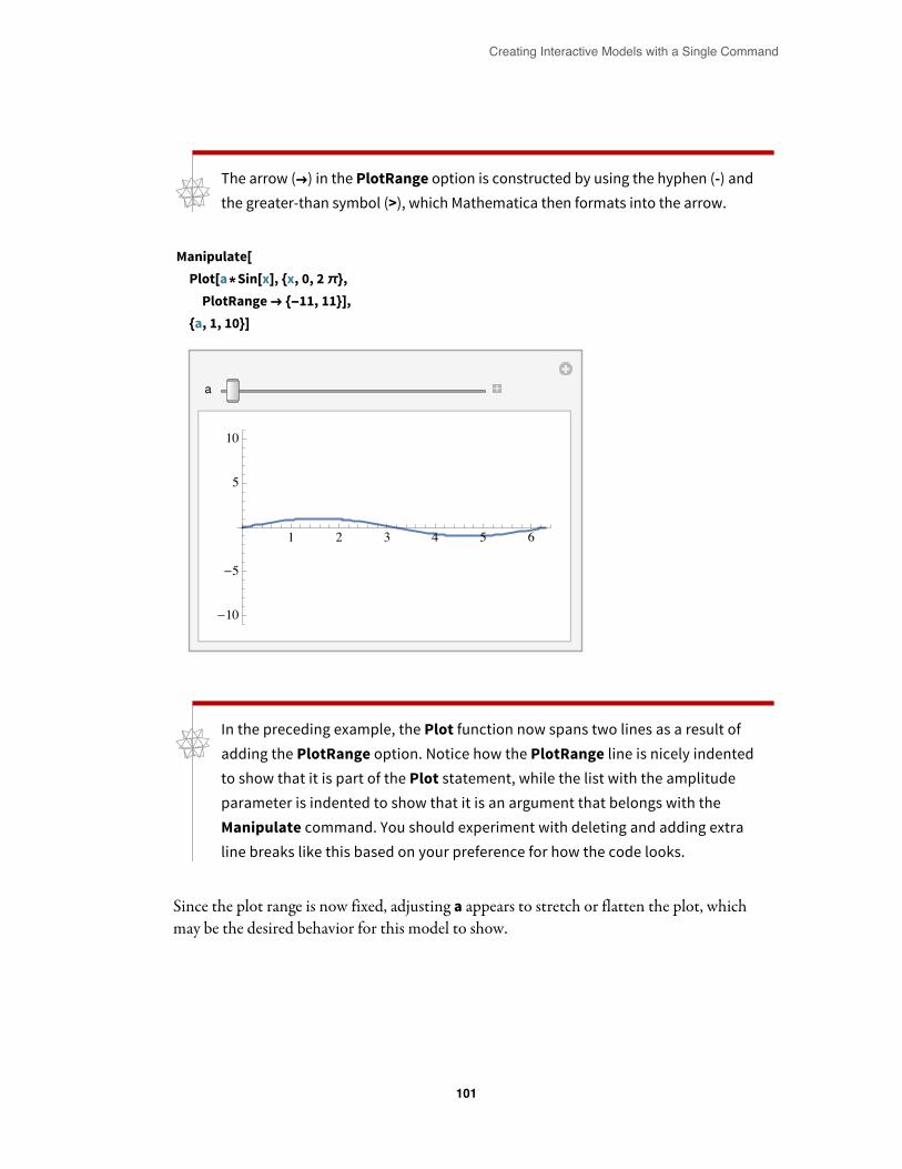
� The arrow (→) in the PlotRange option is constructed by using the hyphen (-) andthe greater-than symbol (>), which Mathematica then formats into the arrow.

Manipulate[Plot[a*Sin[x], {x, 0, 2π},PlotRange→ {-11, 11}],

{a, 1, 10}]

�

� � � � � �

-��

-�

�

��

� In the preceding example, the Plot function now spans two lines as a result ofadding the PlotRange option. Notice how the PlotRange line is nicely indentedto show that it is part of the Plot statement, while the list with the amplitudeparameter is indented to show that it is an argument that belongs with theManipulate command. You should experiment with deleting and adding extraline breaks like this based on your preference for how the code looks.

Since the plot range is now fixed, adjusting a appears to stretch or flatten the plot, whichmay be the desired behavior for this model to show.

�������� ����������� ������ ���� � ������ �������

���

Optimizing Performance for 3D Graphics

When 3D graphics are manipulated with controllers like slider bars, they may appearjagged while the controllers are being moved, and then smooth again when the controllersare released. The following example shows this behavior in action.

Manipulate[Plot3D[Sin[a x y], {x, -2, 2}, {y, -2, 2}],{a, 1, 5}]

�

Mathematica's default behavior is to optimize the performance while the controller is beingmoved, and then to optimize the appearance once the controller is released. This allows afast interaction between users and the controllers, and nicely rendered results when fin-ished. However, if rendering is more important than fast interaction, then the use ofoptions like PerformanceGoal can be handy.

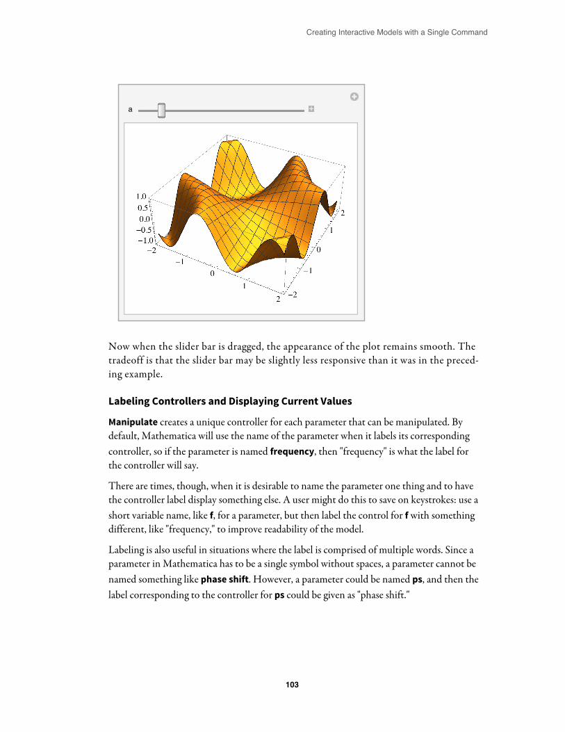
Manipulate[Plot3D[Sin[a x y], {x, -2, 2}, {y, -2, 2}, PerformanceGoal→ "Quality"],{a, 1, 5}]

������� �

���

�

Now when the slider bar is dragged, the appearance of the plot remains smooth. Thetradeoff is that the slider bar may be slightly less responsive than it was in the preced-ing example.

Labeling Controllers and Displaying Current Values

Manipulate creates a unique controller for each parameter that can be manipulated. Bydefault, Mathematica will use the name of the parameter when it labels its correspondingcontroller, so if the parameter is named frequency, then "frequency" is what the label forthe controller will say.

There are times, though, when it is desirable to name the parameter one thing and to havethe controller label display something else. A user might do this to save on keystrokes: use ashort variable name, like f, for a parameter, but then label the control for f with somethingdifferent, like "frequency," to improve readability of the model.

Labeling is also useful in situations where the label is comprised of multiple words. Since aparameter in Mathematica has to be a single symbol without spaces, a parameter cannot benamed something like phase shift. However, a parameter could be named ps, and then thelabel corresponding to the controller for ps could be given as "phase shift."

�������� ����������� ������ ���� � ������ �������

���

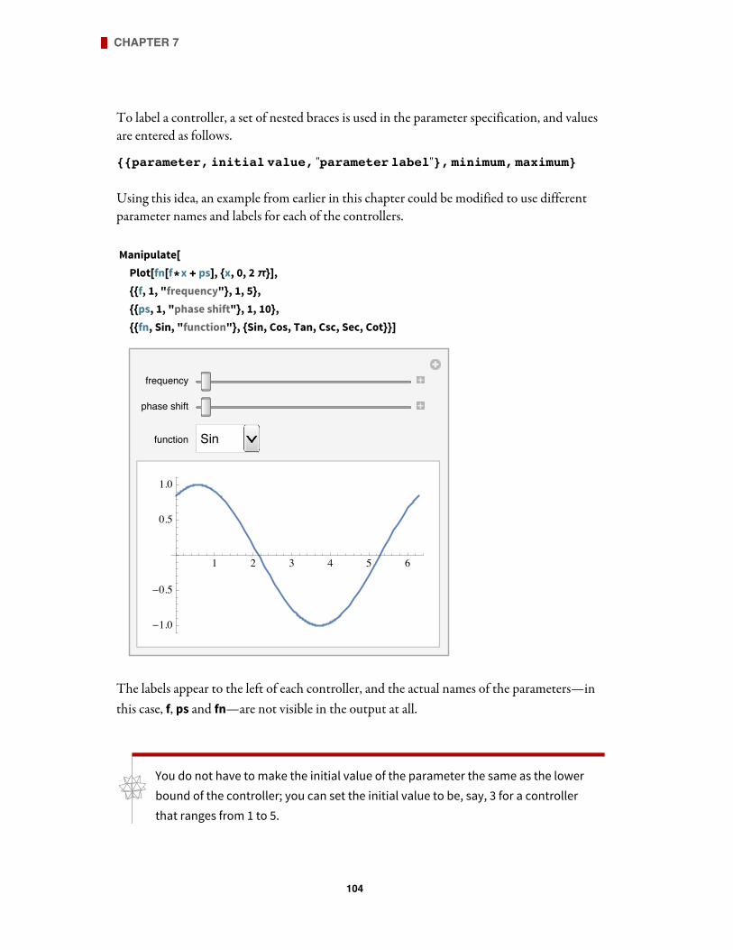
To label a controller, a set of nested braces is used in the parameter specification, and valuesare entered as follows.

������������ ������� ������ "��������� �����"�� �������� ��������

Using this idea, an example from earlier in this chapter could be modified to use differentparameter names and labels for each of the controllers.

Manipulate[Plot[fn[f*x + ps], {x, 0, 2π}],{{f, 1, "frequency"}, 1, 5},{{ps, 1, "phase shift"}, 1, 10},{{fn, Sin, "function"}, {Sin, Cos, Tan, Csc, Sec, Cot}}]

���������

����� �����

�������� ���

� � � � � �

-���

-���

���

���

The labels appear to the left of each controller, and the actual names of the parameters—inthis case, f, ps and fn—are not visible in the output at all.

� You do not have to make the initial value of the parameter the same as the lowerbound of the controller; you can set the initial value to be, say, 3 for a controllerthat ranges from 1 to 5.

������� �

���

Another useful option to set for the controllers is Appearance→"Labeled", which willdisplay the current value of the parameter to the right of its Animation Controls button.(There is no need to set this option for the fn parameter, since the function name is alreadydisplayed within the controller as part of the buttons.)

Manipulate[Plot[fn[f*x + ps], {x, 0, 2π}],{{f, 1, "frequency"}, 1, 5, Appearance→ "Labeled"},{{ps, 1, "phase shift"}, 1, 10, Appearance→ "Labeled"},{{fn, Sin, "function"}, {Sin, Cos, Tan, Csc, Sec, Cot}}]

��������� �

����� ����� �

�������� ���

� � � � � �

-���

-���

���

���

Creating an Interactive Plot Label

While labeling individual controllers in aManipulate can be useful, it can also be desirableto create an interactive plot label that takes all of these labels into consideration and printsa single expression, like the equation of the function being graphed.

The following example plots Sin[f*x], where f is a manipulable parameter. The controllerfor f uses the Appearance→"Labeled" option setting to print its values to the right of thecontroller, which is helpful, but the user is still required to examine the code to ascertainexactly what function is being plotted.

�������� ����������� ������ ���� � ������ �������

���

Manipulate[Plot[Sin[f*x], {x, 0, 2π}],{{f, 1, "frequency"}, 1, 5, Appearance→ "Labeled"}]

��������� �

� � � � � �

-���

-���

���

���

Creating an interactive plot label can make the function being plotted more obvious. First,a quick explanation of the PlotLabel option is necessary. PlotLabel is an option for Plot(and other plotting commands) that prints a label at the top of the plot. PlotLabel expectsa string to be passed as its option setting. A string in Mathematica is enclosed with quota-tion marks.

Plot[Sin[x], {x, 0, 2π}, PlotLabel→ "My plot of sin(x)"]

� � � � � �

-���

-���

���

����� ���� �� ���(�)

Strings can also be joined together with the <> operator. This is useful when construct-ing a single string from multiple pieces of information that might be coming fromdifferent places.

������� �

���

Plot[Sin[x], {x, 0, 2π}, PlotLabel→ "My plot of " <> "sin(x)"]

� � � � � �

-���

-���

���

����� ���� �� ���(�)

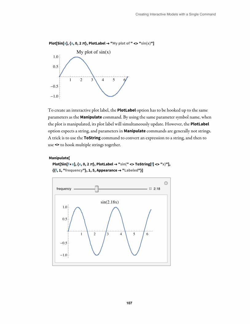
To create an interactive plot label, the PlotLabel option has to be hooked up to the sameparameters as theManipulate command. By using the same parameter symbol name, whenthe plot is manipulated, its plot label will simultaneously update. However, the PlotLabeloption expects a string, and parameters inManipulate commands are generally not strings.A trick is to use the ToString command to convert an expression to a string, and then touse <> to hook multiple strings together.

Manipulate[Plot[Sin[f*x], {x, 0, 2π}, PlotLabel→ "sin(" <> ToString[f] <> "x)"],{{f, 1, "frequency"}, 1, 5, Appearance→ "Labeled"}]

��������� ����

� � � � � �

-���

-���

���

������(�����)

�������� ����������� ������ ���� � ������ �������

���

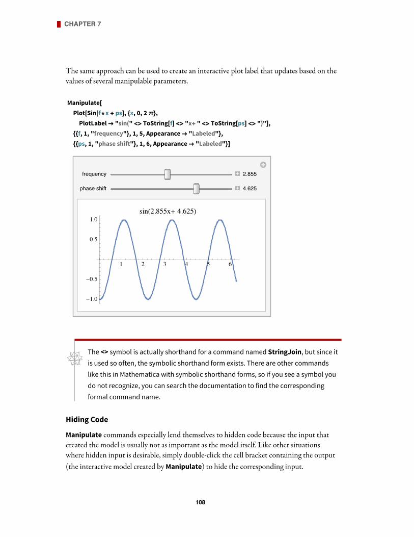
The same approach can be used to create an interactive plot label that updates based on thevalues of several manipulable parameters.

Manipulate[Plot[Sin[f*x + ps], {x, 0, 2π},PlotLabel→ "sin(" <> ToString[f] <> "x+ " <> ToString[ps] <> ")"],

{{f, 1, "frequency"}, 1, 5, Appearance→ "Labeled"},{{ps, 1, "phase shift"}, 1, 6, Appearance→ "Labeled"}]

��������� �����

����� ����� �����

� � � � � �

-���

-���

���

������(������+ �����)

� The <> symbol is actually shorthand for a command named StringJoin, but since itis used so often, the symbolic shorthand form exists. There are other commandslike this in Mathematica with symbolic shorthand forms, so if you see a symbol youdo not recognize, you can search the documentation to find the correspondingformal command name.

Hiding Code

Manipulate commands especially lend themselves to hidden code because the input thatcreated the model is usually not as important as the model itself. Like other situationswhere hidden input is desirable, simply double-click the cell bracket containing the output(the interactive model created byManipulate) to hide the corresponding input.

������� �

���

Manipulate[Plot[a*Sin[f*x + ps], {x, 0, 2π}, PlotRange→ 6],{{f, 1, "frequency"}, 1, 5, Appearance→ "Labeled"},{{a, 3, "amplitude"}, 1, 5, Appearance→ "Labeled"},{{ps, 0, "phase shift"}, 0, 2π, Appearance→ "Labeled"}]

��������� �

��������� �

����� ����� �

� � � � � �

-�

-�

-�

�

�

�

Obfuscating code can be taken one step further by deleting the input entirely or by copyingand pasting just the output (the interactive model) into a separate notebook. In many cases,the interactive model will still function when the notebook is opened, although it will notbe operational if it references a function or data that is no longer available at the time offuture reuse. The next section outlines ways to makeManipulate statements self-containedso that they include all necessary definitions.

� Double-clicking the output to hide the input is muchmore common than deleting it.If you keep the input intact, you can addminor edits later quite easily. If the input isdeleted, you would likely have to start over and recreate theManipulate statement.

�������� ����������� ������ ���� � ������ �������

���

Remembering User-Defined Functions

While the examples so far have utilizedWolfram Language functions, theManipulatecommand can be used with any expression, including user-defined functions. Once afunction is defined, thenManipulate can operate on it. As an example, the function f[x] isdefined as follows.

f[x_] := 2 x2 + 2 x + 1

� Remember, you can typeset an exponent using the Ctrl+6 keyboard shortcut or byusing one of the palettes to create a typesetting template.

And now this function can be used withManipulate.

Manipulate[Plot[f[a*x], {x, -4, 4}, PlotRange→ {0, 25}],{a, -1, 1}]

�

-� -� � � �

�

��

��

��

��

������� �

���

If the output cell of the above expression—the interactive model created byManipulate—was copied to a new notebook, and the Mathematica session was ended, and the newnotebook was reopened later, then the interactive model would no longer function becauseMathematica would not remember the definition of the function f.

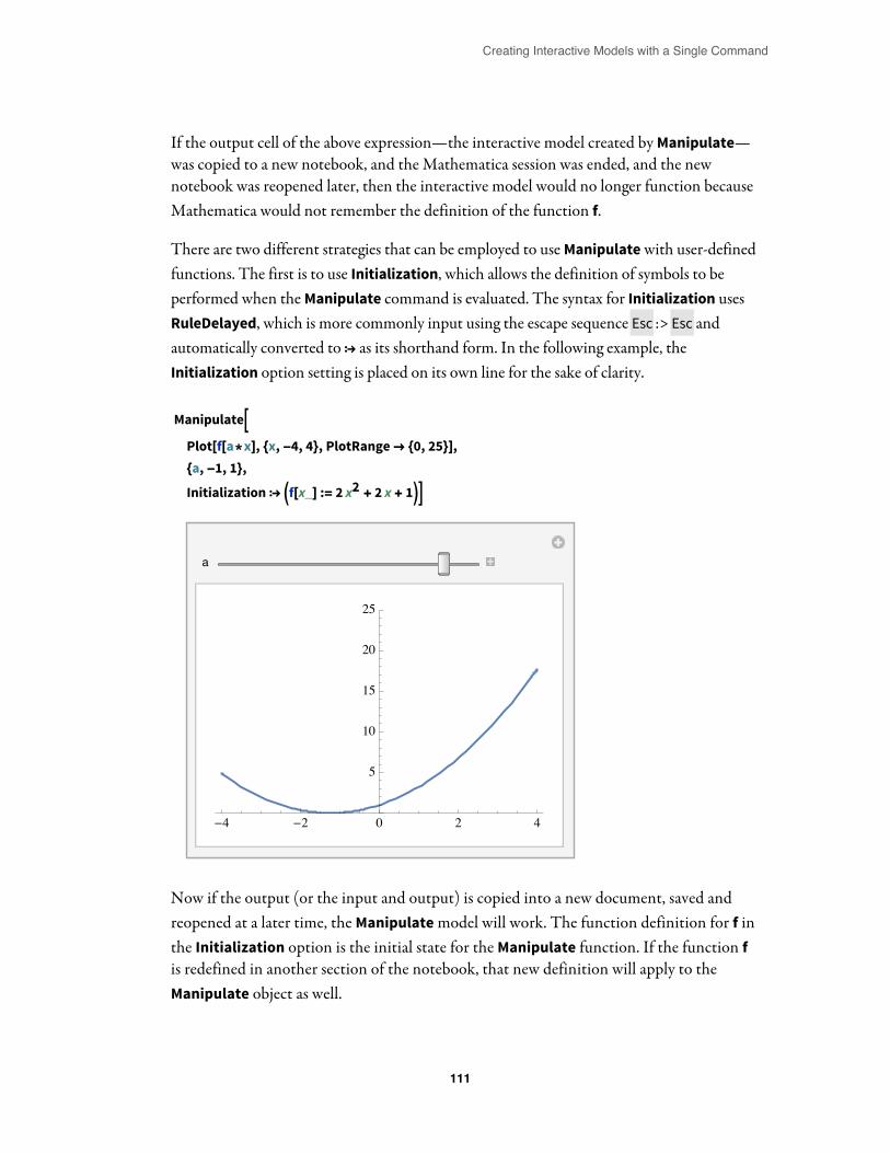
There are two different strategies that can be employed to useManipulatewith user-definedfunctions. The first is to use Initialization, which allows the definition of symbols to beperformed when theManipulate command is evaluated. The syntax for Initialization usesRuleDelayed, which is more commonly input using the escape sequence Esc :>Esc andautomatically converted to⧴ as its shorthand form. In the following example, theInitialization option setting is placed on its own line for the sake of clarity.

Manipulate

Plot[f[a*x], {x, -4, 4}, PlotRange→ {0, 25}],{a, -1, 1},Initialization⧴ f[x_] := 2 x2 + 2 x + 1

�

-� -� � � �

�

��

��

��

��

Now if the output (or the input and output) is copied into a new document, saved andreopened at a later time, the Manipulatemodel will work. The function definition for f inthe Initialization option is the initial state for the Manipulate function. If the function fis redefined in another section of the notebook, that new definition will apply to theManipulate object as well.

�������� ����������� ������ ���� � ������ �������

���

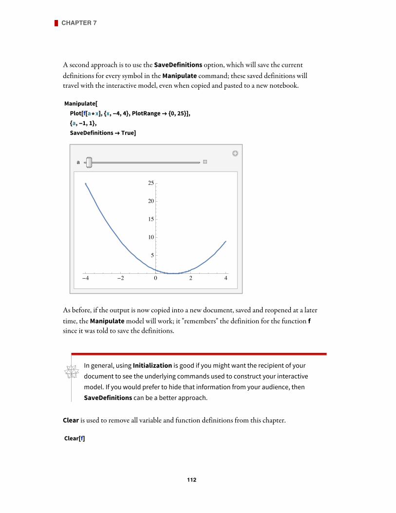
A second approach is to use the SaveDefinitions option, which will save the currentdefinitions for every symbol in theManipulate command; these saved definitions willtravel with the interactive model, even when copied and pasted to a new notebook.

Manipulate[Plot[f[a*x], {x, -4, 4}, PlotRange→ {0, 25}],{a, -1, 1},SaveDefinitions→ True]

�

-� -� � � �

�

��

��

��

��

As before, if the output is now copied into a new document, saved and reopened at a latertime, theManipulatemodel will work; it "remembers" the definition for the function fsince it was told to save the definitions.

� In general, using Initialization is good if you might want the recipient of yourdocument to see the underlying commands used to construct your interactivemodel. If you would prefer to hide that information from your audience, thenSaveDefinitions can be a better approach.

Clear is used to remove all variable and function definitions from this chapter.

Clear[f]

������� �

���

ConclusionThe use ofManipulate to communicate ideas is quite popular withMathematica users, sincethe results can be immediately understood without the audience having to understand oreven see anyWolfram Language commands. A good understanding and generous use ofManipulate can go a long way in explaining ideas, illustrating concepts and simulatingphenomena—and all with a single command!

Exercises1. Create a Manipulate statement to vary x2 + 1, where x is an integer ranging

from 1 to 10.

2. Similarly to Exercise 1, create aManipulate statement to produce a list of values of theform {x, x2 + 1, x3 + 1}, where x is an integer ranging from 1 to 10.

3. Create aManipulate statement to show the list of {x, x2 + 1, x3 + 1} and then add afourth element to the list that is an expression that answers whether x2 > 2 x+ 1. Asbefore, use the same integer range of 1 to 10 for the variable x.

4. Use the Wolfram Language to create a plot of x2 + 3 x - 1 over the domain from-5 to 5.

5. UseManipulate to visualize the behavior of x2 + 3 x- 1 when a constant c is used tomultiply x2, and where c ranges from 1 to 20.

6. When moving the slider from the example in Exercise 5, remember that Mathematicais choosing the optimal plot range as the slider is moved. Use PlotRange to introducea fixed plot range of -5 to 100.

7. Copy the input from Exercise 6 and add a second constant d to change 3 x to 3 d x,where d also ranges from 0 to 20.

8. Copy the input from Exercise 7 and add another function so that you are visualizingboth c x2 + 3 d x- 1 and 2 c x2 - d x+ 3. (Reminder: to visualize two functions on thesame set of axes, place the functions in a list.)

9. Use the ThermometerGauge command to create a gauge illustrating the temperatureof 10 on a scale of 0 to 50.

10. Now useManipulate to create a model of the temperature 10 x, where x can bechanged from 0 to 5.

�������� ����������� ������ ���� � ������ �������

���