AN ABSTRACT OF THE THESIS OF

Xiaoliang He for the degree of Master of Science in Mechanical Engineering

presented on January 4, 2013

Title: CFD Simulation of Single-Phase and Flow Boiling in Confined Jet Impingement with in-Situ Vapor Extraction Using Two Kinds of Multiphase Models

Abstract approved: _______________________________________

Deborah V. Pence

With continued development of the electronic industry, the demand for highly efficient heat

removal solutions requires innovative cooling technologies. A computational fluid dynamic

(CFD) study, including heat transfer, is performed for an axisymmetric, confined jet

impingement experiencing boiling and coupled with vapor extraction. Boiling occurs at the

target surface while extraction occurs at the wall confining the radial flow. The region

between the target and confining wall is defined as a confined gap. Extraction is employed to

enhance heat transfer and to minimize the potential negative influence of flow instabilities

resulting from two-phase flow within a confined region.

A three-dimensional sector of the confined jet is employed in the simulation. A single

circular impinging jet with a constant jet diameter (4 mm) and variable gap height (0.5, 1.0

and 1.5 mm), also known as nozzle-to-target spacing, is considered. The effect of mass flux at

the confined gap entrance is also investigated (200, 400 and 800 kg/m2-s) for a range of heat

flux (5 to 50 W/cm2).

Fluid flow and heat transfer are simulated using the Volume of Fluid (VOF) model and the

wall-boiling sub-model within the Multiphase Segregated Flow (MSF) model. The boiling

sub-model in the VOF model applies the Rohsenow boiling correlation, while in the MSF

model, the Kurul-Podowski boiling sub-model is used. Also, vapor extraction is realized by

different mechanisms for these two models. For the VOF model, a specific phase “wall

porosity” can be assigned to a wall to make it porous. Over a range of pressure differentials

across this porous wall such that the inertial transport influence is negligible, vapor transport

should agree with Darcy’s law. For the MSF model, a wall can be made permeability to one

substance or phase while remaining impermeable to the other substance or phase. However, a

portion of the substance or phase reaching the boundary allowed to pass through the surface

must be specified. A pressure drop cannot be applied across the wall, thereby prohibiting

Darcy flow modeling. The solutions of both models are at steady state.

The boiling curves without vapor extraction from both models are provided and compared

to experiments. Simulations matching experimental wall temperatures under-predict

theoretical vapor generation and those matching vapor generation over-estimate wall

superheat. For cases with no extraction, local temperature and velocity profiles from the VOF

model are provided at several radial locations within the confined gap. Scalar temperature and

pressure distributions and velocity vectors are presented to explain observations in profiles.

© Copyright by Xiaoliang He

January 4, 2013

All Rights Reserved

CFD Simulation of Single-Phase and Flow Boiling in Confined Jet Impingement with

in-Situ Vapor Extraction Using Two Kinds of Multiphase Models

by

Xiaoliang He

A THESIS

submitted to

Oregon State University

in partial fulfillment of

the requirements for the

degree of

Master of Science

Presented January 4, 2013

Commencement June 2013

Master of Science thesis of Xiaoliang He presented on January 4, 2013.

APPROVED:

_____________________________________________________________________

Major Professor, representing Mechanical Engineering

_____________________________________________________________________

Head of the School of Mechanical, Industrial, and Manufacturing Engineering

_____________________________________________________________________

Dean of the Graduate School

I understand that my thesis will become part of the permanent collection of Oregon

State University libraries. My signature below authorizes release of my thesis to any

reader upon request.

_____________________________________________________________________

Xiaoliang He, Author

ACKNOWLEDGEMENTS

I would like to express my sincere gratitude to Dr. Deborah V. Pence for her guidance

and support during my graduate study. I would also like to thank my graduate

committee members: Dr. James Liburdy, Dr. Vinod Narayanan and Dr. Wade Marcum

(GCR), for serving on my committee and assisting in several phases of the research

process. Last, the greatest appreciation is for my parents, for their encouragement and

support during this study. Additionally, I would like to thank Saran Salakijs,

Christopher Stull, Nick Cappello, Randall Fox, and Adam Damiano for their selfless

assistance.

TABLE OF CONTENTS Page

Chapter 1 – Introduction ............................................................................................................. 1

Chapter 2 – Literature Review.................................................................................................... 3

2.1 Single-Phase Confined Impinging Jets ....................................................................... 3

2.1.1 Single-Phase Experimental Studies .................................................................... 3

2.1.2 Single-Phase Computational Studies .................................................................. 7

2.2 Two-Phase Impinging Jets........................................................................................ 12

2.2.1 Two-Phase Experimental Studies ..................................................................... 12

2.2.2 Two-Phase Computational Studies ................................................................... 14

2.3 Mass Extraction through Porous Membranes ........................................................... 15

2.3.1 Experimental Extraction Studies ...................................................................... 15

2.3.2 Computational Extraction Studies .................................................................... 19

Chapter 3 – Problem Statement ................................................................................................ 20

3.1 General Hypothesis .................................................................................................. 20

3.2 Simulation Objectives............................................................................................... 20

3.2.1 Simulating single-phase confined impinging jets ............................................. 20

3.2.2 Simulating flow boiling in the confined impinging jets ................................... 21

3.2.3 Simulating vapor extraction .............................................................................. 21

3.3 Geometric Configuration .......................................................................................... 22

3.3.1 Computational domain ...................................................................................... 23

3.3.2 Computational mesh ......................................................................................... 24

3.3.3 Boundary conditions ......................................................................................... 25

Chapter 4 – Physical and Computational Models .................................................................... 27

4.1 Governing Equations of VOF model ........................................................................ 27

4.1.1 Conservation Equations of Mass and Momentum ............................................ 28

4.1.2 Energy Conservation Equation ......................................................................... 29

4.1.3 Volume Fraction Transport Equation ............................................................... 29

4.1.4 Phase Interaction Parameters ............................................................................ 29

4.1.5 Boiling Model ................................................................................................... 30

4.1.6 Wall Porosity Model ......................................................................................... 31

TABLE OF CONTENTS (Continued) Page

4.2 Governing Equations of Multiphase Segregated Fluid Model ................................. 31

4.2.1 Conservation Equations of Mass and Momentum ............................................ 32

4.2.2 Energy Equation ............................................................................................... 33

4.2.3 Standard k-ε Model ........................................................................................... 33

4.2.4 Phase Interaction Models .................................................................................. 35

4.2.5 Boiling Model ................................................................................................... 40

4.2.6 Wall Permeability Model .................................................................................. 44

4.2.7 Computational Details ...................................................................................... 44

Chapter 5 – Data Reduction and CFD Validation .................................................................... 46

5.1 Data Reduction ......................................................................................................... 46

5.1.1 Area-averaged wall temperatures ..................................................................... 46

5.1.2 Dimensionless variables ................................................................................... 47

5.2 Residual and grid refinement convergence ............................................................... 48

5.3 Turbulent kinetic energy and dissipation .................................................................. 49

5.4 Validation ................................................................................................................. 49

Chapter 6 – Result and Discussion ........................................................................................... 53

6.1 Parametric study of VOF results .................................................................................... 53

6.1.1 Influence of mass flux ............................................................................................. 54

6.1.2 Influence of heat flux ............................................................................................... 66

6.1.3 Influence of gap height ............................................................................................ 75

6.2 Vapor extraction ............................................................................................................. 82

6.3 Multiphase segregated flow results ................................................................................ 83

6.4 Discussion....................................................................................................................... 86

Chapter 7 – Conclusions and Recommendations ..................................................................... 88

Bibliography ............................................................................................................................. 90

APPENDICES .......................................................................................................................... 94

LIST OF FIGURES

Figure Page

3.1 Cross section of the experimental test part ........................................................................ 22

3.2 Schematic of flow field ...................................................................................................... 23

3.3 Schematic of the heat block ............................................................................................... 23

3.4 Mesh of fluid domain ......................................................................................................... 24

3.5 Mesh of impinging part ..................................................................................................... 25

3.6 Mesh of flow channel ........................................................................................................ 25

3.7 Schematic of boundary conditions ..................................................................................... 26

5.1 Schematic of sectors for area-averaged temperature ......................................................... 47

5.2 Quality at outlet, Xout, versus heat flux, q″, for the base case including theoretical

predictions and simulations from both the VOF and MSF simulations ............................ 50

5.3 Area-averaged wall superheat for CFD and experimental results ..................................... 51

6.1 Dimensionless fluid temperature distributions, T*, as a function of dimensionless

radial distance, r* , for three mass flux values (G = 200, 400, and 800 kg/s-m2): (a)

z* ≈ 1, (b) z* = 0.5, and (c) z* ≈ 0. ....................................................................................55

6.2 Volume fraction of vapor, α, as a function of dimensionless radial distance, r* , near

z* ≈ 0 and for three mass flux values (G = 200, 400, and 800 kg/s-m2). ..........................57

6.3 Volume fraction of vapor, α, contours for three mass flux values: (a) 200 kg/s-m2,

(b) 400 kg/s-m2, and (c) 800 kg/s-m2 ...............................................................................59

6.4 Velocity vector fields for three mass flux values: (a) 200 kg/s-m2, (b) 400 kg/s-m2,

and (c) 800 kg/s-m2 ...........................................................................................................61

6.5 Dimensionless fluid temperature profiles, T*, as a function of dimensionless

distance above the target plate, z*, for three mass flux values (G = 200, 400, and 800

kg/s-m2): (a) r* = 0, (b) r* = 1, (c) r* = 2, (d) r* = 4, and (e) r* = 8 ................................63

6.6 Dimensionless radial velocity profiles, ∗, as a function of dimensionless distance

above the target plate, z*, at r* = 2 for three mass flux values (G = 200, 400, and

800 kg/s-m2). .....................................................................................................................65

6.7 Average wall superheat, − , as a function of mass flux, G ...................................66

LIST OF FIGURES (Continued)

Figure Page

6.8 Dimensionless fluid temperature distributions, T*, as a function of dimensionless

radial distance, r* , for five heat flux values (q″ = 5, 10, 20, 30, 50 W/cm2): (a) z* ≈

1, (b) z* = 0.5, and (c) z* ≈ 0. ............................................................................................68

6.9 Volume fraction of vapor, α, as a function of dimensionless radial distance, r* , near

z* ≈ 0 and for five heat flux values (q″ = 5, 10, 20, 30, 50 W/cm2)..................................69

6.10 Velocity vector fields for two heat flux values: (a) 5 W/cm2 (b) 10 W/cm2 (c) 20

W/cm2 (d) 30 W/cm2 and (e) 50 W/cm2 ........................................................................71

6.11 Dimensionless fluid temperature profiles, T*, as a function of dimensionless

distance above the target plate, z*, for five heat flux values (q″ = 5, 10, 20, 30, 50

W/cm2): (a) r* = 0, (b) r* = 1, (c) r* = 2, (d) r* = 4, and (e) r* = 8 .................................73

6.12 Dimensionless radial velocity profiles, ∗, as a function of dimensionless

distance above the target plate, z*, for five heat flux values (q″ = 5, 10, 20, 30, 50

W/cm2): (a) r* = 1 and (b) r* = 2 ......................................................................................74

6.13 Dimensionless fluid temperature distributions, T*, as a function of dimensionless

radial distance, r* , for three gap heights (Z = 0.5, 1.0 and 1.5 mm): (a) z* ≈ 1, (b) z*

= 0.5, and (c) z* ≈ 0. ..........................................................................................................76

6.14 Volume fraction of vapor, α, as a function of dimensionless radial distance, r* , near

z* ≈ 0 and for three gap heights (Z = 0.5, 1.0 and 1.5 mm). ..............................................78

6.15 Dimensionless fluid temperature profiles, T*, as a function of dimensionless

distance above the target plate, z*, for three gap heights (Z = 0.5, 1.0 and 1.5 mm):

(a) r* = 0 and (b) r* = 2 .....................................................................................................79

6.16 Dimensionless radial velocity profiles, ∗, as a function of dimensionless distance

above the target plate, z*, for three gap heights (Z = 0.5, 1.0 and 1.5 mm) at r* = 2. .......79

6.17 Velocity vector fields for three gap heights: (a) 0.5 mm, (b) 1.0 mm,

and (c) 1.5 mm ...................................................................................................................81

6.18 Average wall superheat, − , as a function of gap height, Z. ...............................82

6.19 Near wall fluid temperature distributions, T, as a function of dimensionless radial

distance, r* , for with and without vapor extraction ...........................................................83

LIST OF FIGURES (Continued)

Figure Page

6.20 Volume fraction of vapor, α, contours for the base case using: (a) VOF model and

(b) MSF model ...................................................................................................................84

6.21 Velocity vector fields for the base case: (a) mixture velocity using VOF model, (b)

liquid velocity using MSF model and (c) vapor velocity using MSF model .....................85

LIST OF TABLES

Table Page

4.1 Drag force coefficients in Eqn. (4-23) for Red ≤ 450 .......................................................... 37

6.1 Test conditions .................................................................................................................... 53

Nomenclature

A Area (m2)

cp Specific heat (kJ/kg-K)

CD Drag coefficient

d Diameter (m)

f Bubble departure frequency (Hz)

F Force (N)

G Mass flux (kg/m2-s)

g Gravitational constant (m/s2)

H Total enthalpy (kJ/kg)

h Heat transfer coefficient (W/m2-K)

i Enthalpy (kJ/kg)

K Thermal conductivity (W/m-K)

k Turbulent kinetic energy (m2/s2)

l Length scale (m)

nˮ The density of nucleation sites (/m2)

Nu Nusselt number

m Mass flow rate (kg/s)

P Pressure (kPa)

Pr Prandtl number

Q Diffusive heat transfer (kJ/kg)

qˮ Heat flux (W/m2)

r Radius (m)

Re Reynolds number

S Source term

T Temperature (K)

U Total energy (kJ/kg)

u Velocity in x direction (m/s)

V Velocity (m/s)

v Velocity in y direction (m/s)

w Velocity in z direction (m/s)

X Quality

Z Distance between the parallel plates (m)

Greek Letters and Symbols

Δ Difference

∇ Gradient

∇⦁ Divergence

α Volume fraction

β Viscous resistance

µ Dynamic viscosity (kg/m-s)

ρ Density (kg/m3)

σ Surface tension (N/m)

τ Stress tensor

Inertia resistance

Viscous dissipation rate (m2/s3)

θ The liquid-vapor contact angles (degree)

λ′ The length scale of the cavity (m)

γ The permeability factor of the wall

Ω The angle of the slice in units of radians

Homogeneous quality

Subscripts

c Continuous phase (liquid)

d Dispersed phase (vapor)

conv Convection

evap Evaporation

i Phase i (liquid)

in Inlet

j Phase j (vapor)

l Liquid

n Normal direction

out Outlet

sat Saturation

t Turbulent

U Energy

V Momentum

v Vapor

w Wall

Superscripts

* Theoretical value

t Turbulent

D Drag

VM Virtual mass

L Lift

TD Turbulent dispersion

Others

qbw Surface heat flux due to boiling (W/m2)

hlat Latent heat of vaporization (kJ/kg)

Cqw An empirical coefficient in Rohsenow correlation

np Prandtl number exponent in Rohsenow correlation

Cew A constant regulating the amount of heat flux used to generate vapor

, Effective thermal conductivity (W/m-K)

Gk Turbulent production

lcd The Kurul-Podowski length scale (m)

The symmetric particle interaction area density (/m2)

EOAW Eotvos number

Kdry The fraction of the surface in contact with vapor

dw Bubble departure diameter (m)

Rc The critical cavity radius (m)

Time between bubble departure and nucleation of the next bubble (s)

Area-averaged wall temperature (K)

1

Chapter 1 – Introduction

With the continued development of the electronics industry, an advanced cooling solution is

still in great demand. Though the scale of the electronic devices becomes smaller and smaller,

their energy consumption remains high, which aggravates a common problem, that is,

insufficient cooling. Existing cooling scheme limitations constrains further development of

electronics in certain fields. Thus, the mission of searching for innovative techniques of heat

dissipation for small-scale objects remains necessary and to some industries, is considered

urgent.

Depending upon the constraints imposed and heat flux dissipation needs, single-phase flows

may be sufficient to achieve the desired goals. For these cooling schemes, the driving

temperature difference drives the cooling. To enhance heat transfer microscale geometries

might be considered, such as in microchannel heat sinks. For such devices, the surface area

and heat transfer coefficient are both improved.

For higher heat flux needs, either cryogenics with their extremely low operating

temperatures or two-phase flows with their latent energy potential might be more suitable.

Associated with cryogenics are extremely low operating temperatures, which may cause

condensation from the air near the electronics. On the other hand, two-phase flows have their

own set of issues, depending upon the operating scale. For small scale devices, such as

microchannel heat sinks, flow instabilities and large pressure gradients can result from phase

change. To achieve the benefits of small scale geometries and their enhanced heat transfer

coefficients, yet avoid flow instabilities and large pressure gradients, two-phase flow in a

2

confined radial jet is considered. The general configuration of a confined radial jet is naturally

stabilizing and the increased area alleviates somewhat the pressure drop due to phase change.

To further stabilize the flow and provide the opportunity to enhance the heat transfer, the

confinement surface can be made hydrophobic and porous. Drawing a vacuum at the backside

of the confining plate allows for vapor to be extracted from the confined gap rather than

moved through the gap. Experimental studies in a test device with no opportunities for local

measurements or visual observations are currently underway. Therefore, a computational

study is warranted.

Required is a study of the relevant literature in which to place the present study. Included are

experimental and computational studies focused on single-phase, confined impingement from

a single circular jet. As fewer two-phase studies of this jet configuration are available, some

studies of confined planar jets and submerged radial jets are included. Finally, two-phase

computational flow studies of this configuration are lacking. This is believed to be the first

study proposed to assess heat transfer and fluid flow in a confined radial impinging jet

experiencing two-phase laminar flow. Note that the laminar flow restriction is based on single-

phase liquid velocities throughout. Extraction studies, with and without phase change, have

been computationally studied in microchannel configurations, but not in a jet configuration.

3

Chapter 2 – Literature Review

High flux, compact heat sinks are needed to operate electronics within their temperature

limits. One means of accomplishing cooling is by way of an axisymmetric impinging jet. The

three main types of impinging jets are free, submerged and confined. The working fluid can be

either a gas or a liquid. In the case of liquid jets, the jet can remain in liquid phase or undergo

phase change.

Adding a confining surface parallel to the impingement surface and at a plane coincident

with the jet exit provides an opportunity for improved heat transfer due to recirculation within

the confined gap region. The added benefit of jets undergoing phase change, i.e. two-phase

impinging jets compared with single phase impinging jets, is the higher heat fluxes due to

latent energy transfer and uniformity of surface temperature. Removal of bubbles from the

heat transfer surface can be enhanced by making the confining surface hydrophobic porous

and drawing a vacuum on the opposite side of the porous surface.

Addressed in the review of the literature are experimental papers specific to confined jets.

Computational papers reviewed include impinging jets of different configurations. The few

experimental papers and one computational paper regarding vapor extraction are summarized.

2.1 Single-Phase Confined Impinging Jets

Laminar and turbulent single-phase confined jets have been studied experimentally and

computationally. Reviewed are single jets, primarily of circular jet configurations.

2.1.1 Single-Phase Experimental Studies

4

Fitzgerald and Garimella [1] studied single-phase FC-77 impinging flow fields, without

looking into the Nusselt number, using a square edge confined jet with hydraulic diameters

between 3.18 and 6.35 mm. The impingement surface is estimated based on flow field figures

to have a diameter of 140 mm, resulting in impinging surface-to-jet diameter ratios, ds/dj, of

44 and 22 for the two jets, respectively. The diameter of the confined plate is assumed equal to

the impinging surface diameter. Flow fields were acquired using laser-Doppler velocimetry at

flow rates consistent with turbulent flow (4000 ≤ Re ≤ 23,000) at the jet exit and ratios of gap

height over jet diameter, H/dj, of 2, 3, and 4. A recirculation zone observed in the confined gap

region moves radially outward with increases in Reynolds number and with increases in

dimensionless gap height. A maximum in velocity near the wall is observed at an r/r j

approximately equal to 2 and the maximum turbulence levels occur at an r/r j approximately

equal to 4.

In a study using FC-77 leaving a circular confined jet and impinging on a 10 mm square

heater, Garimella and Rice [2] studied heat transfer from the impingement surface held at

constant heat flux. The Reynolds number range was consistent with that of Fitzgerald and

Garimella [1], with a wider range of jet diameters (0.79 to 6.35 mm) and dimensionless gap

heights up to 14. Although not provided, sketches of the experimental facility indicate a

confined gap diameter well in excess that of the jet diameters, with an estimated minimum

possible value of 70 based on a scaled estimate of the polycarbonate insert diameter and the

largest jet diameter considered. For a Reynolds number of 13,000, a jet diameter of 1.59 mm,

and all dimensionless gap heights studied, the maximum local heat transfer coefficient occurs

at the impingement zone. For dimensionless gap heights less than 5, a secondary peak in heat

transfer coefficient is observed. At an H/dj of one, the secondary peak is located near an r/r j

value equal to 4. For an H/dj equal to one, a jet diameter of 3.18 mm, and for Reynolds

5

numbers greater than 17,000, there is a primary off-peak heat transfer coefficient near r/r j

equal to one and a secondary peak around r/r j equal to 3.6. The secondary peak is believed to

be the result of recirculation observed in the confined gap region.

The secondary peak in local Nusselt number observed at r/r j equal to four in Garimella and

Rice [2] is also observed in San et al. [3] even though flow through the confined gap region is

constrained to two opposing dimensions and the working fluid is air. Impinging jet diameters

between 3 and 9 mm and jet Reynolds numbers from 30,000 to 67,000 were studied for a

single dimensionless gap height of 2. The secondary peaks are more obvious for larger jet

diameters and for shorter dimensionless confined gap lengths, L/dj, which vary between 44

and 133.

On the other hand, Koseoglu and Baskaya [4] also using air and a dimensionless gap height

of 2 found the maximum Nusselt number to occur off-axis as opposed to the jet centerline,

near an r/r j approximately equal to 1.2 for a Reynolds number of 10,000. Although at a

Reynolds number 41% lower than Garimella and Rice [2] and 67% lower than that of San et

al. [3], perhaps more influential may be the 100 mm square target plate relative to the 10 mm

diameter jet used by Koseoglu and Baskaya [4], which yields an equivalent ds/dj of 10. This

ratio is considerably smaller than those of works discussed previously.

Colucci and Viskanta [5] also studied air leaving a 1.27 mm diameter confined jet

impinging on a dimensionless target diameter, ds/dj, equal to 8. For dimensionless gap heights

of 0.25 and 1.0 and a Reynolds number of 30,000, which is equal to that of San et al. [3], two

distinct off-center peaks are observed in the local Nusselt number. The peak closest to the

centerline occurs at an r/r j near 1.2 for both gap heights, with the second peak farther

6

downstream in the larger gap height. Recall that San et al. [3] observed the peak at the jet

center.

Chang et al. [6] studied single-phase impingement of R-113 onto a 66.6 mm heater

embedded in a 72 mm diameter target plate. Jet Reynolds numbers varied between 9,800 and

92,500 while dimensionless gap heights varied between 1.5 and 4.0. Although jet diameters of

1, 2 and 4 mm were considered, data for the 4 mm diameter jet show a single maximum in the

local averaged Nusselt number. Local averaged values represent integrated values between the

stagnation point and the local radial location, r. This maximum occurs at the jet centerline for

the entire range of Reynolds numbers: 9,798 to 92,558. It should be noted that the heat transfer

coefficient used in the Nusselt number is defined using the local bulk fluid temperature,

determined using energy balances.

The 4 mm diameter jet and 100 mm equivalent diameter target plate yields a ds/dj of 18,

which is approximately twice that of Colucci and Viskanta [5] with off-axis peaks in local

Nusselt number and approximately half that of Rice and Garimella. Based on the previous

results, it appears that the change between local Nusselt numbers peaking at the centerline

versus peaking at an off-center location may be influenced by the dimensionless target

diameter in addition to the dimensionless gap height and Reynolds number. However, no

conclusions can be drawn. Exiting conditions of the confined gap may also play a role. For

example, the fluid exit configuration in Chang [6] is also considerably different than the

previous four reported works on heat transfer. In these previous studies, flow discharges

radially into the environment at the end of the confined gap region; however, in the work of

Chang et al. [6] the exiting flow is redirected in an annulus back to the supply reservoir.

7

Heat transfer coefficients are computed using an adiabatic wall temperature in San et al. [3].

Colluci and Viskanta [5] demonstrate the appropriateness of using jet exit temperature in lieu

of the adiabatic wall temperature for their test conditions. Garimella and Rice [2] also use the

jet exit temperature whereas Chang et al. [6] base the heat transfer coefficient on the local bulk

fluid temperature determined using an energy balance. Details regarding how Koseoglu and

Baskaya [4] evaluate the heat transfer coefficient are not provided.

Two different local averaged Nusselt number correlations are provided, one for r/r j less than

and the other for r/r j greater than 2.5. A strong recirculation vortex is believed to exist at r/r j

equal to 2.5. Correlations are a function of dimensionless radial distance, dimensionless gap

height and jet Reynolds number correlations are also provided as a function of Prandtl

numbers even though data was acquired for a single fluid, R-113.

Single-phase Nusselt number correlations at the stagnation zone and area averaged values

were developed by Li and Garimella [7]. Nusselt numbers are correlated with Reynolds

number, Prandtl number, dimensionless jet length and dimensionless heater diameters. The

correlation developed for all fluids is valid for the following ranges: Reynolds number (8,500

– 23,000), Prandtl number (0.7 – 25.2), and dimensionless jet length (0.25 – 12). Jet lengths

and heater diameters (11.28 – 22.56 mm) are scaled by the jet diameter (1.59 – 12.7 mm).

Heat transfer coefficients as a function of radial location are provided, showing a marked

increase with jet velocity and a mild increase with decreasing gap heights.

2.1.2 Single-Phase Computational Studies

Heat transfer using a single confined impinging has been simulated for single-phase flows

under both turbulent flow conditions and laminar flow conditions. A review of existing

correlations for predicting jet impingement heat transfer and a comparison of various

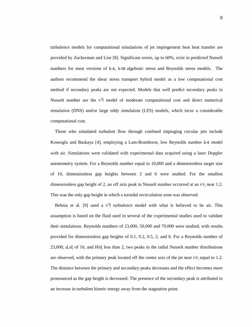
8

turbulence models for computational simulations of jet impingement heat heat transfer are

provided by Zuckerman and Lior [8]. Significant errors, up to 60%, exist in predicted Nusselt

numbers for most versions of k-ε, k-ω algebraic stress and Reynolds stress models. The

authors recommend the shear stress transport hybrid model as a low computational cost

method if secondary peaks are not expected. Models that well predict secondary peaks in

Nusselt number are the v2f model of moderate computational cost and direct numerical

simulation (DNS) and/or large eddy simulation (LES) models, which incur a considerable

computational cost.

Those who simulated turbulent flow through confined impinging circular jets include

Koseoglu and Baskaya [4], employing a Lam-Bramhorst, low Reynolds number k-ε model

with air. Simulations were validated with experimental data acquired using a laser Doppler

anemometry system. For a Reynolds number equal to 10,000 and a dimensionless target size

of 10, dimensionless gap heights between 2 and 6 were studied. For the smallest

dimensionless gap height of 2, an off axis peak in Nusselt number occurred at an r/r j near 1.2.

This was the only gap height in which a toroidal recirculation zone was observed.

Behnia et al. [9] used a v2f turbulence model with what is believed to be air. This

assumption is based on the fluid used in several of the experimental studies used to validate

their simulations. Reynolds numbers of 23,000, 50,000 and 70,000 were studied, with results

provided for dimensionless gap heights of 0.1, 0.2, 0.5, 2, and 6. For a Reynolds number of

23,000, ds/dj of 10, and H/dj less than 2, two peaks in the radial Nusselt number distributions

are observed, with the primary peak located off the center axis of the jet near r/r j equal to 1.2.

The distance between the primary and secondary peaks decreases and the effect becomes more

pronounced as the gap height is decreased. The presence of the secondary peak is attributed to

an increase in turbulent kinetic energy away from the stagnation point.

9

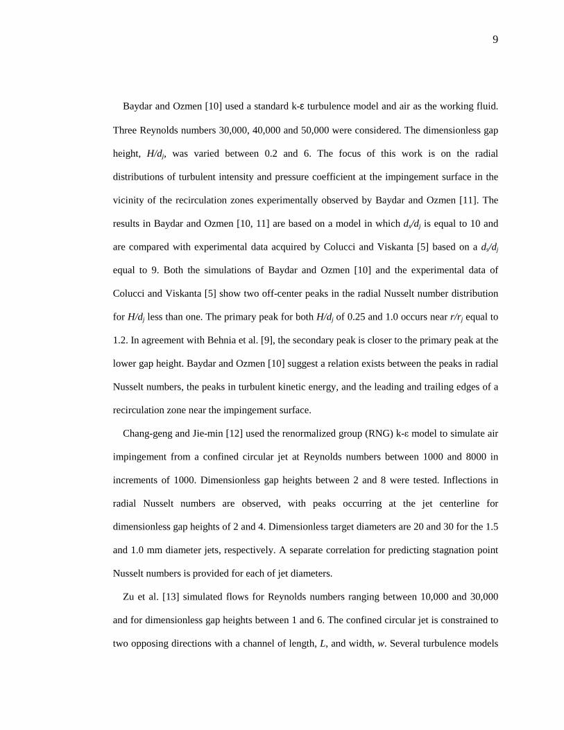
Baydar and Ozmen [10] used a standard k-ε turbulence model and air as the working fluid.

Three Reynolds numbers 30,000, 40,000 and 50,000 were considered. The dimensionless gap

height, H/dj, was varied between 0.2 and 6. The focus of this work is on the radial

distributions of turbulent intensity and pressure coefficient at the impingement surface in the

vicinity of the recirculation zones experimentally observed by Baydar and Ozmen [11]. The

results in Baydar and Ozmen [10, 11] are based on a model in which ds/dj is equal to 10 and

are compared with experimental data acquired by Colucci and Viskanta [5] based on a ds/dj

equal to 9. Both the simulations of Baydar and Ozmen [10] and the experimental data of

Colucci and Viskanta [5] show two off-center peaks in the radial Nusselt number distribution

for H/dj less than one. The primary peak for both H/dj of 0.25 and 1.0 occurs near r/r j equal to

1.2. In agreement with Behnia et al. [9], the secondary peak is closer to the primary peak at the

lower gap height. Baydar and Ozmen [10] suggest a relation exists between the peaks in radial

Nusselt numbers, the peaks in turbulent kinetic energy, and the leading and trailing edges of a

recirculation zone near the impingement surface.

Chang-geng and Jie-min [12] used the renormalized group (RNG) k-ε model to simulate air

impingement from a confined circular jet at Reynolds numbers between 1000 and 8000 in

increments of 1000. Dimensionless gap heights between 2 and 8 were tested. Inflections in

radial Nusselt numbers are observed, with peaks occurring at the jet centerline for

dimensionless gap heights of 2 and 4. Dimensionless target diameters are 20 and 30 for the 1.5

and 1.0 mm diameter jets, respectively. A separate correlation for predicting stagnation point

Nusselt numbers is provided for each of jet diameters.

Zu et al. [13] simulated flows for Reynolds numbers ranging between 10,000 and 30,000

and for dimensionless gap heights between 1 and 6. The confined circular jet is constrained to

two opposing directions with a channel of length, L, and width, w. Several turbulence models

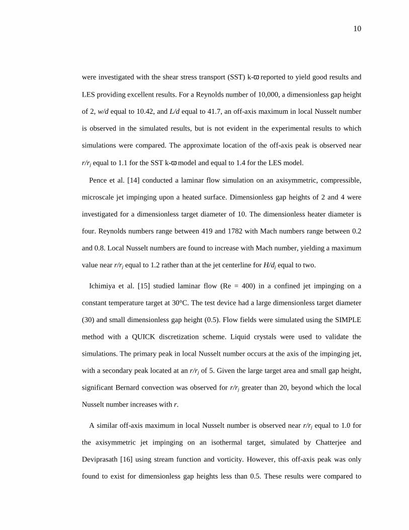
10

were investigated with the shear stress transport (SST) k-ω reported to yield good results and

LES providing excellent results. For a Reynolds number of 10,000, a dimensionless gap height

of 2, w/d equal to 10.42, and L/d equal to 41.7, an off-axis maximum in local Nusselt number

is observed in the simulated results, but is not evident in the experimental results to which

simulations were compared. The approximate location of the off-axis peak is observed near

r/r j equal to 1.1 for the SST k-ω model and equal to 1.4 for the LES model.

Pence et al. [14] conducted a laminar flow simulation on an axisymmetric, compressible,

microscale jet impinging upon a heated surface. Dimensionless gap heights of 2 and 4 were

investigated for a dimensionless target diameter of 10. The dimensionless heater diameter is

four. Reynolds numbers range between 419 and 1782 with Mach numbers range between 0.2

and 0.8. Local Nusselt numbers are found to increase with Mach number, yielding a maximum

value near r/r j equal to 1.2 rather than at the jet centerline for H/dj equal to two.

Ichimiya et al. [15] studied laminar flow (Re = 400) in a confined jet impinging on a

constant temperature target at 30°C. The test device had a large dimensionless target diameter

(30) and small dimensionless gap height (0.5). Flow fields were simulated using the SIMPLE

method with a QUICK discretization scheme. Liquid crystals were used to validate the

simulations. The primary peak in local Nusselt number occurs at the axis of the impinging jet,

with a secondary peak located at an r/r j of 5. Given the large target area and small gap height,

significant Bernard convection was observed for r/r j greater than 20, beyond which the local

Nusselt number increases with r.

A similar off-axis maximum in local Nusselt number is observed near r/r j equal to 1.0 for

the axisymmetric jet impinging on an isothermal target, simulated by Chatterjee and

Deviprasath [16] using stream function and vorticity. However, this off-axis peak was only

found to exist for dimensionless gap heights less than 0.5. These results were compared to

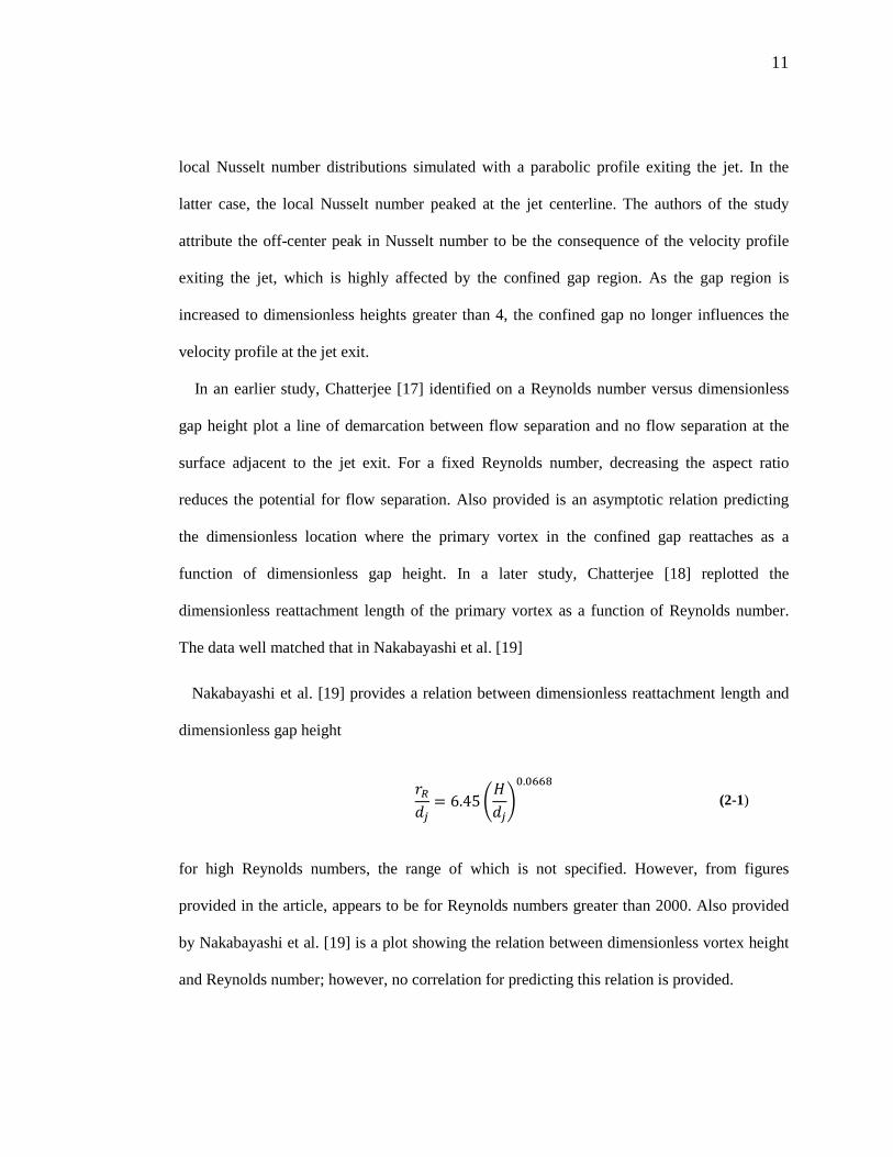
11

local Nusselt number distributions simulated with a parabolic profile exiting the jet. In the

latter case, the local Nusselt number peaked at the jet centerline. The authors of the study

attribute the off-center peak in Nusselt number to be the consequence of the velocity profile

exiting the jet, which is highly affected by the confined gap region. As the gap region is

increased to dimensionless heights greater than 4, the confined gap no longer influences the

velocity profile at the jet exit.

In an earlier study, Chatterjee [17] identified on a Reynolds number versus dimensionless

gap height plot a line of demarcation between flow separation and no flow separation at the

surface adjacent to the jet exit. For a fixed Reynolds number, decreasing the aspect ratio

reduces the potential for flow separation. Also provided is an asymptotic relation predicting

the dimensionless location where the primary vortex in the confined gap reattaches as a

function of dimensionless gap height. In a later study, Chatterjee [18] replotted the

dimensionless reattachment length of the primary vortex as a function of Reynolds number.

The data well matched that in Nakabayashi et al. [19]

Nakabayashi et al. [19] provides a relation between dimensionless reattachment length and

dimensionless gap height

!"# = 6.45 )*"#+,.,--.

(2-1)

for high Reynolds numbers, the range of which is not specified. However, from figures

provided in the article, appears to be for Reynolds numbers greater than 2000. Also provided

by Nakabayashi et al. [19] is a plot showing the relation between dimensionless vortex height

and Reynolds number; however, no correlation for predicting this relation is provided.

12

A study by Biswas et al. [20] includes plots similar to those in Nakabayashi et al. [19], i.e.

of dimensionless reattachment length and vortex height versus Reynolds number, but do not

compare the results of Nakabayashi et al. [19].

2.2 Two-Phase Impinging Jets

Studies with two-phase confined impinging jets, experimental or computational, are more

limited than those of single-phase studies. Included in this section are papers with jet

configurations other than confined radial jets.

2.2.1 Two-Phase Experimental Studies

Ma and Bergles [21] studied R-113 from a circular jet as it impinged on a completely

submerged heated surface. A definition of incipient boiling is provided, as the influence of jet

velocity and jet subcooling. For given wall superheats, Tw – Tsat, heat flux increases with both.

In fully developed boiling, the influence of both velocity and subcooling are negligible.

Results are compared to pool boiling, from which it is suggested that impingement cooling has

improved cooling capabilities over pool boiling. The considerable effects of surface conditions

are highlighted, even under consistent surface preparation.

Wolf et al. [22] studied axial variations in wall temperature and heat transfer coefficients

using a planar impinging jet with water for a range of velocities. General observations made

by Ma and Bergles [21] regarding subcooling and velocity in the heat transfer regime below

fully developed boiling were confirmed. For heat fluxes lower than those yielding fully

developed boiling, significant streamwise variations in wall temperature and heat transfer

coefficients exist. For fully developed flow, wall surface temperatures are essentially constant

and the influence of velocity is negligible.

13

Shin et al. [23] studied a planar jet for Reynolds numbers of 2000, 3000 and 5000 with

variable dimensionless distances between the jet exit and target plate of 0.5, 1.0 and 4.0.

Reynolds numbers are based on jet diameter, which is also the dimension used to normalize

the jet-to-target distance, for a fluid known as PF5060. In general, heat transfer was enhanced

with increases in jet Reynolds number and smaller distances between the jet exit and target.

However, a dimensionless spacing of unity is deemed the least desirable if trying to avoid

critical heat flux.

Extending their single-phase study, Chang et al. [24] considered heat transfer from a

circular confined jet issuing R-113 as a two-phase mixture of quality 0.20. This allows for an

assumption of saturated flow boiling, conditions under which convection and nucleate-boiling

heat transfer coefficients can be superimposed. Spatial measurements of wall temperature

allowed for assessment radial heat flux and radial heat transfer coefficients, the latter of which

are based on the bulk fluid, or in this case the saturation, temperature. Subtracting from

measured local heat flux the local sub-cooled boiling heat flux predicted using the Rohsenow

correlation from Carey [25] allowed for an assessment of the local two-phase convective heat

transfer. The conclusion is that two-phase convection heat transfer is negligible in comparison

to nucleate boiling heat transfer.

A comprehensive review of jet impingement boiling is provided in Wolf et al. [26].

Highlighted are temperature overshoots by non-wetting fluids, the influence of surface

conditions on boiling curve consistency, significant variations (up to 45°C) in wall

temperature resulting from different modes of heat transfer occurring at different points on the

heated surface, confined jets with nozzle-to-surface spacing resulting in flow acceleration (i.e.,

H/dj ≤ 0.25), and substantial increases in local saturation temperature resulting from a

stagnation pressure significantly higher than the ambient pressure. An example provided by

14

the authors indicates an 11°C increase in saturation temperature resulting from a 47.9 kPa

increase in pressure at the stagnation point for a 10 m/s free jet of saturated water impinging

on the surface. This yields a saturation temperature at the stagnation zone of 111°C compared

with the typical value of 100°C for an ambient pressure of 101.3 kPa. For maximizing the

critical heat flux, a heater over jet diameter ratio of 2.5 is noted.

2.2.2 Two-Phase Computational Studies

Very few computational studies have been conducted on heat transfer using two-phase

impinging jets. The first study discussed is actually a combined analytical/empirical study by

Omar et al. [27]. Provided is an enhanced diffusion model characterizing two-phase heat

transfer enhancement resulting from a free planar impinging jet. The effective diffusivity for

use in the conservation equations is related to jet velocity and jet temperature as well as the

temperature of the impinging surface. Authors anticipate incorporation of the model in

numerical simulations of partial and fully-developed nucleate boiling could significantly

reduce computational costs by avoiding the need for resolving all details of two-phase flow.

Narumanchi et al. [28] simulated nucleate boiling heat transfer in a submerged jet using the

renormalized group k-ε turbulence model. Not all forces are included in their analysis. To

improve predictability, the authors provide a compromise between accuracy and simplicity.

Assumed is a balance between acceleration and gravity forces, based on an assumption that

the diameter of a bubble at lift off and departure are identical. Using differences between

simulations and experiments, two different factors for modifying the bubble departure model

were developed. One corrects the pressure and the other corrects the new wall velocity, both

of which effect bubble size. The model is limited to 20°C wall superheats.

15

A two-dimensional assessment of confined, planar jet impingement with boiling is provided

in Abishek et al. [29]. The focus of the study is the effect of heater-nozzle size ratio on the

heat transfer from a constant temperature heater. A single jet Reynolds number of 2500 is

used with a 20°C subcooling. Heater-nozzle size ratios of 0.5 to 11 and wall superheats

between -5 and 20°C are investigated. A re-normalized group k-ε turbulence model is used in

conjunction with a wall-boiling model. The individual effects of evaporation, convection and

quenching are assessed and a correlation between heater size and wall superheat is provided.

2.3 Mass Extraction through Porous Membranes

2.3.1 Experimental Extraction Studies

Recognizing the potential for gas or vapor bubbles to impede liquid flow in a channel the

size of the bubble, Meng et al. [30] proposed a degassing plate by which to vent the bubbles

from two-phase flow. To ensure bubbles attach to the degassing plate requires the surface

energy to be minimized. This can be accomplished by making the plate hydrophobic in nature,

i.e., the three-phase contact angle must be greater than 90°. Creating carbon dioxide inside the

channels and then venting it through the degassing plate proved the concept. The original

degassing plate was made of silicon with DRIE etched through holes coated with Teflon. The

second design incorporated a commercially available porous Teflon membrane sandwiched

between two DRIE plates.

Later, Meng et al. [31] proposed their concept for application in a microscale methanol fuel

cell. Two commercially available porous membranes were considered: a 1.5 µm pore

polytetrafluoroethylene (PTFE) membrane and a 0.1 µm pore polypropylene membrane.

Membranes were tested with both water and 10-M methanol and were characterized for

robustness. Robustness tests include an investigation of the breakthrough pressure, the

16

pressure differential across the membrane above which leaking occurs. The leakage rate, when

considered for decreasing pressure differentials, was found to follow Darcy’s law.

Nitrogen gas bubbles begin venting immediately upon contact with the membrane if in

water but bubbles travel further downstream and coalesce before being venting from 10-M

methanol. The delay in venting is called the venting threshold, believed to result from either a

thin film between the bubbles and the membrane or tiny droplets trapped in the membrane

pores. Based on experimental data, a one-dimensional gas venting rate model is provided and

related to the driving pressure differential across the membrane, the bubble diameter and the

channel width.

Alyousef and Yao [32] designed and successfully tested a single porous silicon plate that

could pass either de-ionized water through regions containing hydrophilic-coated pores or

carbon dioxide through regions containing hydrophobic-coated pores. The ultimate use for the

plate is in a microscale direct methanol fuel cell.

Xu et al. [33] propose four design criteria for removal of gas bubbles from microchannels

using a porous hydrophobic membrane: (i) channel diameters must be smaller than anticipated

bubble diameters, (ii)the bubble must remain in contact with the membrane long enough to be

extracted, (iii) the bubble must travel slower than a critical velocity above which a film forms

between the membrane and bubble, and (iv) the driving pressure differential applied across the

membrane must be lower than the breakthrough pressure. Equations for each criterion are

provided.

Alexander and Wang [34] proposed use of a hydrophobic porous plate, called a breather, for

extracting vapor from a two-phase microchannel heat sink to minimize the potential for flow

instabilities and liquid dry-out. A correlation was developed to predict extraction rates in

17

terms of a dimensionless pressure ratio, Rp, defined as the pressure drop across the membrane

divided by the pressure drop associated with drag on the bubble. Extraction rates increase with

increases in Rp. For a given pressure differential across the membrane, decreases in liquid

velocity are necessary to increase Rp. Care must be taken to balance the value of Rp and the

liquid velocity needs to achieve desired cooling of the heat sink.

Microchannel flow regimes are provided by David et al. [35] under gas venting and vapor

venting scenarios, for adiabatic and diabatic conditions, respectively. Venting occurs when the

downstream side of the hydrophobic porous membrane is open to the atmosphere. Extraction

rates are reported to be a function of the Weber number, which is shown to have a strong

influence on the flow regime. Higher Weber numbers are associated with annular type flows

where the film in contact with the porous membrane reduces the area of the membrane

exposed to the gas/vapor thereby limiting the amount of possible mass extracted. Flow

regimes for the adiabatic and diabatic conditions under venting are found to differ

significantly.

Advantages of venting a microchannel heat sink under boiling flow conditions include a

potential 60% decrease in channel pressure drop and a lower wall superheat, in which a

maximum of 4.4°C was observed by David et al. [36]. The observed decrease in pressure drop

results from a decrease of mass in the channel but may also be a consequence of change in

flow regime resulting from the decrease of mass in the channel. Given a fixed exit pressure,

the lower channel pressure drop results in a lower inlet pressure and a decrease in saturation

temperature. For a given heat flux and heat transfer coefficient, this results in a lower device

temperature.

18

A two-phase pressure drop model using a separated flow approach is provided. The model

predicts experimental data for mass fluxes near 100 kg/m2-s fairly well but under-predicts data

for higher mass fluxes. A two-phase heat transfer coefficient dependent upon the Martinelli

parameter and single-phase fully developed heat transfer coefficient is also provided. Model

predictions suggest an increase in heat transfer coefficients with venting. Predictions are less

accurate at the lowest mass flux near 100 kg/m2-s and believed to be a result of a stratified

flow condition existing in the presence of the hydrophobic membrane. Stratified flow heat

transfer coefficients are lower than those with churn and annular flows, which are the flow

regimes most typical for higher mass fluxes for channels with the porous membrane

configuration.

The effects of temperature on permeability of porous membranes are reported in Marconnet

et al. [37]. Intrinsic and fluid-specific permeabilities are reported for air and steam. Decreases

in fluid-specific permeability observed with increases in temperature cannot be accounted for

solely as a function of variation in fluid properties. Flows that agree with Darcy’s transport

law should result in intrinsic permeabilities that are independent of temperature.

Intrinsic permeability according to Darcy’s model is a function of the membrane only,

independent of the fluid properties and the flow rate. However, the intrinsic permeability for

air and steam were found to be different, and the intrinsic permeability was found to vary

when heated for both air and steam. Changes in intrinsic permeability were less influenced

when cooled, than when heated. For membranes in which the intrinsic permeability increased

with heating, the departure from Darcy law predictions is hypothesized to be a result of

membrane deflection, which can result in an increase in pore size. Intrinsic permeability is

directly proportional to the pore diameter squared. A significant difference in temperature

experienced across the membrane and a lag in membrane temperature compared with that of

19

the fluid temperature are proposed as a possible explanation as to the differences in

permeability observed for the same membrane when heated compared with that when cooled.

2.3.2 Computational Extraction Studies

Fang et al. [38] simulated three-dimensional transient vapor-venting from a microchannel

with one wall made of a hydrophobic porous membrane. A volume of fluid (VOF) method

was employed coupled with a capillary force model and interphase mass transfer. The flow

regime changes resulting from mass extraction are demonstrated and compared to flow

regimes with no venting. The wall temperature remains lower for a longer section of

microchannel when vapor is vented than when no vapor is vented. Simulated pressure drop

across the microchannel as a function of heat flux is shown to plateau for the venting case

whereas the pressure drop continues to increase in a microchannel with no venting. Although

the pressure drop is decreased, pressure fluctuations are greater in the venting channel than in

the non-vented microchannel. High frequency low amplitude pressure fluctuations are

attributed to bubble expansion whereas venting was found to result in lower frequency high

amplitude fluctuations. To consider the influence of condensation on the venting process, a

heat sink experiencing 0.5 W/cm2 was simulated at the top surface of the membrane. Vapor

venting is reduced when liquid water exists in the membrane. A recommendation is made to

maintain a temperature higher than the saturation temperature.

20

Chapter 3 – Problem Statement

3.1 General Hypothesis

According to the literature, confined impinging jets offer efficient heat removal for certain

geometry devices. Compared to single-phase flow, two-phase flow provides superior heat

transfer performance due to both thermodynamic and hydrodynamic reasons. However, the

problems brought about from flow boiling, such as phase change pressure drop along the flow

channel, vapor accumulation, etc., may affect the flow pattern and consequently the heat

transfer performance. Experimental confined jet studies have shown that vapor extraction

coupled with flow boiling can improve the heat removal capability. However, few

computational studies on either two-phase flow boiling in confined jets or vapor extraction

from flow boiling have been published. The present study includes a computational

investigation in which the influences of geometry and inertia on two-phase heat transfer are

considered.

3.2 Simulation Objectives

The present study involves several aspects of simulating confined impinging jets, including

(1) single-phase flow, (2) flow boiling and (3) vapor extraction.

3.2.1 Simulating single-phase confined impinging jets

The single-phase confined impinging jet simulation serves the role of validation and

baseline data for which to compare flow boiling and flow boiling with extraction cases. The

computational model developed here is used with little modification for flow boiling

situations. Furthermore, using single-phase flow results as initial starting solutions provides

for a comparatively easier converged solution in proceeding to higher heat flux, that is, to two-

phase flow scenarios.

21

3.2.2 Simulating flow boiling in the confined impinging jets

Simulating the flow boiling that occurs within the confined gap is a crucial part of the

project. Two kinds of boiling models are considered here. One is the “volume of fluid” (VOF)

model, the other is a multiphase segregated flow (MSF) formulation that employs a “wall

boiling” model. Detailed descriptions of these two models are provided in Chapter 4. The

basic goals of a good boiling simulation are (1) to yield a good prediction of wall superheat,

and (2) to yield theoretical vapor generation.

3.2.3 Simulating vapor extraction

Simulation of vapor extraction is based on the solution from flow boiling. Therefore,

accuracy of the flow boiling results can significantly impact the solution of vapor extraction.

In a corresponding experiment, a hydrophobic membrane is used to separate the vapor phase

from the two-phase liquid-plus-vapor phase mixture within the confined gap. By all accounts,

vapor transport through the membrane is expected to follow Darcy’s law. However, how

vapor extraction can be modeled varies between the two flow boiling models. In Star-CCM+

version 7.04, the commercially available software used throughout the investigation, a specific

phase “wall porosity” can be assigned for the VOF model. Options also exist for

characterizing the hydrophobicity of this surface. For a given range of pressure differentials

across the porous wall and with the inertial transport influence neglected, vapor transport

should agree with Darcy’s law. Driven by the desire for a steady state solution, no interfaces

are being tracked. Therefore, with a sufficient applied pressure differential, the theoretical

amount of vapor generated, assuming it reaches the extraction surface, should be extracted.

For the “wall boiling” model, a wall can be made permeability to one substance while

remaining impermeable to the other substance. However, no pressure drop can be applied

22

across the wall, prohibiting Darcy flow modeling. Rather a “wall permeability factor” must be

set. This factor controls the amount of the permeable phase in contact with the wall that is

permitted to transport through the wall. As a result, the extraction rate cannot be predicted.

Rather the wall permeability factor must be guessed and iteratively improved until the

extracted vapor matches that of the experimental results.

3.3 Geometric Configuration

A cross-sectional view of the radial confined jet test device is shown Figure 3.1. The radii

of the jet and the impingement surface are held fixed throughout the study at 2 mm and 19

mm, respectively. The gap height is allowed to vary from 0.5 mm to 1.5 mm. Cartridge heaters

supply energy to the aluminum block serving as the impingement surface. The confining

surface of the confined jet is formed with a porous Teflon membrane supported by a

perforated plastic plate. Further details of the experimental test device are provided in Sabo

[39].

Figure 3.1 Cross section of the experimental test part

23

3.3.1 Computational domain

The basic geometry of the computational domain includes a three-dimensional (3-D), 10-

degree sector of the radial jet, the impingement surface and the radial confined gap. Although

the flow should exist primarily in two dimensions, the radial and axial directions, vapor

extraction simulations require a surface; hence, a 3-D domain in studied.

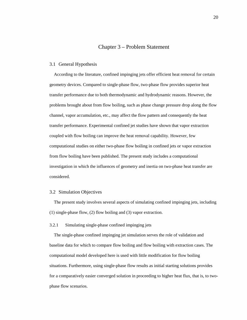
The flow field of the combined jet and confined gap constitute the “fluid” region of the

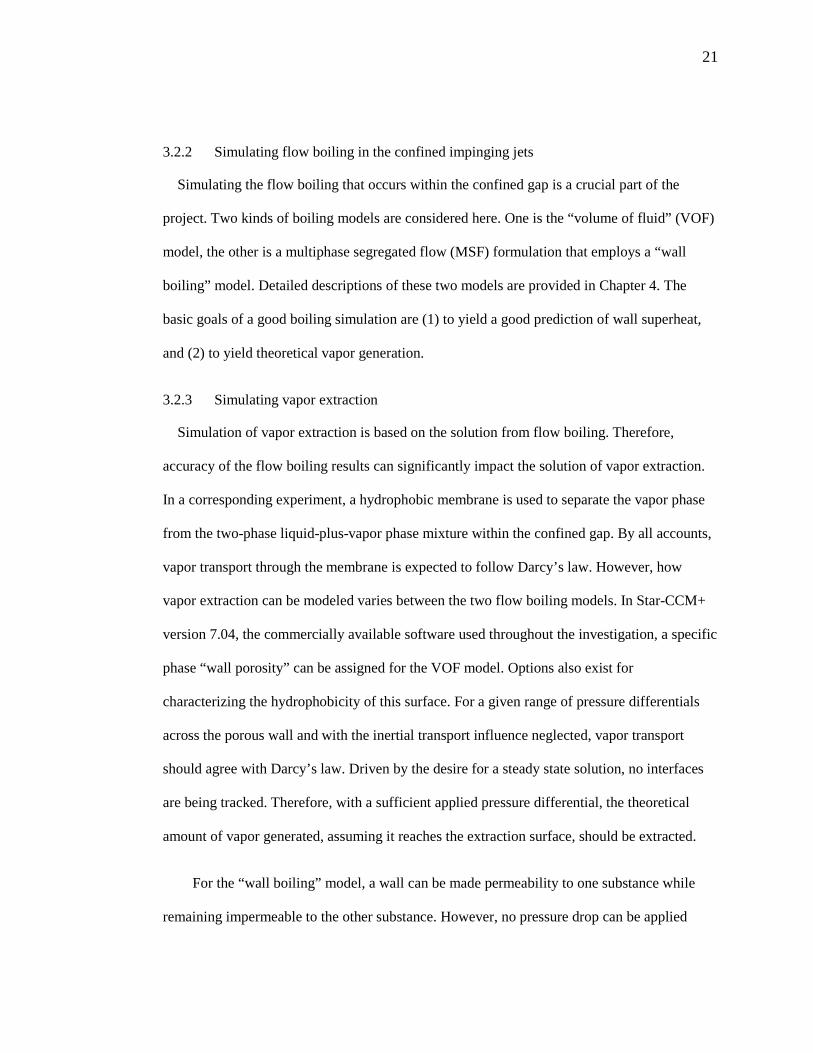
computational domain, which is shown in Figure 3.2. The portion of the heater block above

the cartridge heater is shown in Figure 3.3 and constitutes the “solid” region of the

computational domain. Sub-cooled liquid water enters the inlet of the radial jet, as shown in

Figure 3.2, flows through the jet, impinges on the heated surface, then is heated as it flows

radially through the confined gap before leaving at the designated outlet. The heater block

plays the dual role of impingement surface and heat source. A constant heat flux is assigned at

the bottom portion of the heater block. Including a portion of the heater block allows for an

average wall temperature that more closely mimics the experimental conditions than does the

average wall temperature from assigning a constant heat flux directly to the surface

constraining the bottom of the flow field.

Figure 3.2 Schematic of flow field Figure 3.3 Schematic of the heat block

24

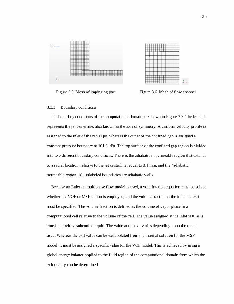
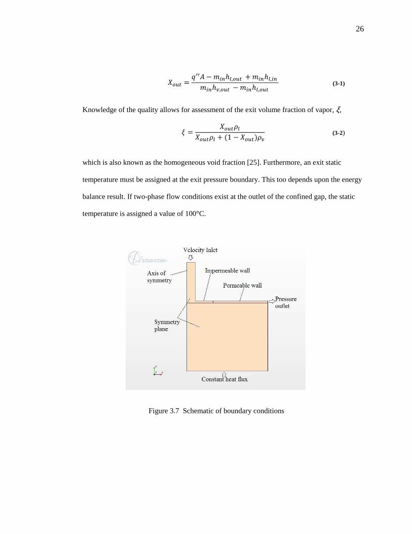
3.3.2 Computational mesh

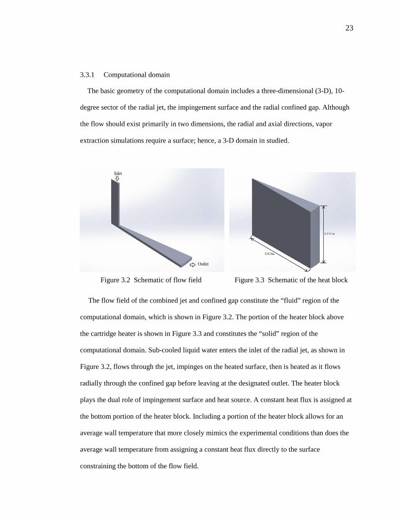
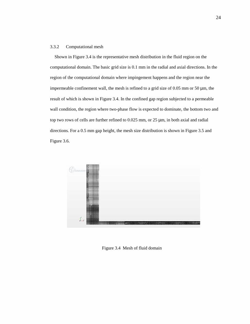
Shown in Figure 3.4 is the representative mesh distribution in the fluid region on the

computational domain. The basic grid size is 0.1 mm in the radial and axial directions. In the

region of the computational domain where impingement happens and the region near the

impermeable confinement wall, the mesh is refined to a grid size of 0.05 mm or 50 µm, the

result of which is shown in Figure 3.4. In the confined gap region subjected to a permeable

wall condition, the region where two-phase flow is expected to dominate, the bottom two and

top two rows of cells are further refined to 0.025 mm, or 25 µm, in both axial and radial

directions. For a 0.5 mm gap height, the mesh size distribution is shown in Figure 3.5 and

Figure 3.6.

Figure 3.4 Mesh of fluid domain

25

Figure 3.5 Mesh of impinging part

Figure 3.6 Mesh of flow channel

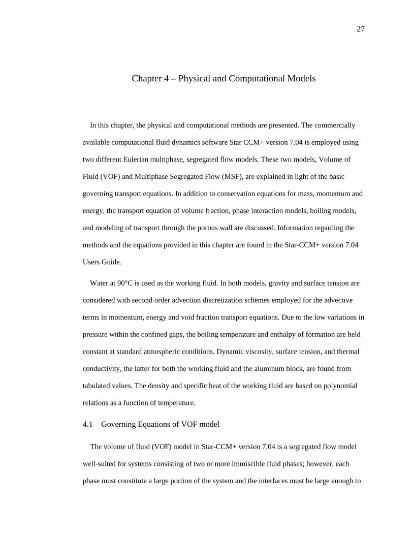
3.3.3 Boundary conditions

The boundary conditions of the computational domain are shown in Figure 3.7. The left side

represents the jet centerline, also known as the axis of symmetry. A uniform velocity profile is

assigned to the inlet of the radial jet, whereas the outlet of the confined gap is assigned a

constant pressure boundary at 101.3 kPa. The top surface of the confined gap region is divided

into two different boundary conditions. There is the adiabatic impermeable region that extends

to a radial location, relative to the jet centerline, equal to 3.1 mm, and the “adiabatic”

permeable region. All unlabeled boundaries are adiabatic walls.

Because an Eulerian multiphase flow model is used, a void fraction equation must be solved

whether the VOF or MSF option is employed, and the volume fraction at the inlet and exit

must be specified. The volume fraction is defined as the volume of vapor phase in a

computational cell relative to the volume of the cell. The value assigned at the inlet is 0, as is

consistent with a subcooled liquid. The value at the exit varies depending upon the model

used. Whereas the exit value can be extrapolated from the internal solution for the MSF

model, it must be assigned a specific value for the VOF model. This is achieved by using a

global energy balance applied to the fluid region of the computational domain from which the

exit quality can be determined

26

/012 = 3445 − 67ℎ9,012 + 67ℎ9,7 67ℎ;,012 − 67ℎ9,012 (3-1)

Knowledge of the quality allows for assessment of the exit volume fraction of vapor, ξ,

= /012<9/012<9 + (1 − /012)<; (3-2)

which is also known as the homogeneous void fraction [25]. Furthermore, an exit static

temperature must be assigned at the exit pressure boundary. This too depends upon the energy

balance result. If two-phase flow conditions exist at the outlet of the confined gap, the static

temperature is assigned a value of 100°C.

Figure 3.7 Schematic of boundary conditions

27

Chapter 4 – Physical and Computational Models

In this chapter, the physical and computational methods are presented. The commercially

available computational fluid dynamics software Star CCM+ version 7.04 is employed using

two different Eulerian multiphase, segregated flow models. These two models, Volume of

Fluid (VOF) and Multiphase Segregated Flow (MSF), are explained in light of the basic

governing transport equations. In addition to conservation equations for mass, momentum and

energy, the transport equation of volume fraction, phase interaction models, boiling models,

and modeling of transport through the porous wall are discussed. Information regarding the

methods and the equations provided in this chapter are found in the Star-CCM+ version 7.04

Users Guide.

Water at 90°C is used as the working fluid. In both models, gravity and surface tension are

considered with second order advection discretization schemes employed for the advective

terms in momentum, energy and void fraction transport equations. Due to the low variations in

pressure within the confined gaps, the boiling temperature and enthalpy of formation are held

constant at standard atmospheric conditions. Dynamic viscosity, surface tension, and thermal

conductivity, the latter for both the working fluid and the aluminum block, are found from

tabulated values. The density and specific heat of the working fluid are based on polynomial

relations as a function of temperature.

4.1 Governing Equations of VOF model

The volume of fluid (VOF) model in Star-CCM+ version 7.04 is a segregated flow model

well-suited for systems consisting of two or more immiscible fluid phases; however, each

phase must constitute a large portion of the system and the interfaces must be large enough to

28

be resolved by the grid. The VOF is a homogenous model; hence, all phases share the same

velocity, pressure, and temperature. The model solves each transport equation using bulk

thermophysical properties. The bulk thermophysical properties of the mixture are determined

by the property and volume fraction of each constituent. For example, density and specific

heat are determined by

where αi is the volume fraction of constituent i and is defined by @ = ABA where for two

phases, as is the case for the present study, ∑ @ = 1DEF .

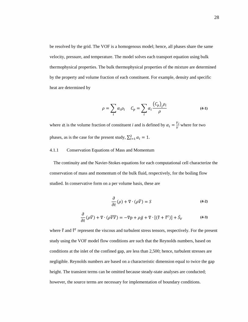
4.1.1 Conservation Equations of Mass and Momentum

The continuity and the Navier-Stokes equations for each computational cell characterize the

conservation of mass and momentum of the bulk fluid, respectively, for the boiling flow

studied. In conservative form on a per volume basis, these are

GG (<) + ∇ ∙ (<IJ) = K (4-2)

GG (<IJ) + ∇ ∙ (<IIJJJJ) = −∇p + <M + ∇ ∙ O(P + P2)R + KA (4-3)

where P and P2 represent the viscous and turbulent stress tensors, respectively. For the present

study using the VOF model flow conditions are such that the Reynolds numbers, based on

conditions at the inlet of the confined gap, are less than 2,500; hence, turbulent stresses are

negligible. Reynolds numbers are based on a characteristic dimension equal to twice the gap

height. The transient terms can be omitted because steady-state analyses are conducted;

however, the source terms are necessary for implementation of boundary conditions.

< = S @< TU = S @ VTUW<<

(4-1)

29

4.1.2 Energy Conservation Equation

The differential form of the energy equation, needed for modeling VOF phase change, and

written in conservative form is

GG (<X) + ∇ ∙ (<*IJ) + ∇ ∙ (IJY)= ∇ ∙ (∇) + ∇ ∙ (P ∙ IJ) + Z ∙ IJ + K[

(4-4)

For incompressible flow analyses, as is the case of the current situation where density is a

function of temperature but not pressure, the term ∇ ∙ (IJY) goes away. Because of the low

velocities, the viscous effects are negligible. Due to the presence of phase change, the buoyant

forces are of importance.

For heat transfer through the solid substrate, only the thermal diffusion term in Equation

(4-4) remains, as does the source term for those cells adjacent to the bottom surface of the

aluminum block where heat is applied.

4.1.3 Volume Fraction Transport Equation

In addition to the conservation of mass, momentum and energy, the transport of each

volume fraction must also be solved when using the VOF model. In differential form the

equation is

GG (@) + ∇ ∙ (@IJ) = K\ (4-5)

4.1.4 Phase Interaction Parameters

As the interface is not tracked in this analysis, there is no need for a phase interaction

model. However, liquid is defined as the continuous phase whereas vapor is defined as the

dispersed phase.

30

4.1.5 Boiling Model

Boiling takes place at a solid surface once the wall temperature exceeds the saturation

temperature. By how much the wall temperature must exceed the saturation temperature to

initiate boiling depends upon heat flux and surface condition. Hence, a relation between the

applied heat flux and the wall superheat, Tw−Tsat, is needed. However, no universally accepted

relation exists. The model available in Star-CCM+ version 7.04 selected for this study is the

subcooled pool boiling correlation by Rohsenow as reported in [25]:

3] = μ9ℎ92_M(<9 − <;)` a TU,9( − b2)Tcℎ92 d 97e fg.,g

(4-6)

where µl, Cp,l, ρl, and Prl are the dynamic viscosity, specific heat, density and Prandtl number

of the liquid phase, respectively. The exponent np acts on the Prandtl number exponent and is

1.7 by default, M is gravity, <; is the vapor phase density, ` is the surface tension coefficient

at the liquid-vapor interface, is the wall temperature and Tc is an empirical coefficient

that varies depending upon the fluid-surface combination. The value of Cqw and np used for the

present investigation were experimentally determined by Sabo [39] to be 0.016 and 1.26.

The size, number and spatial distribution of individual nucleation sites have a significant

influence on the amount of vapor generated. As these numbers are not known for the

particular surface under investigation, nor are they easily simulated, the following relation

6; = T3]ℎ92 (4-7)

can be used to approach the theoretically expected vapor generation by varying Cew, which is a

model constant that regulates the amount of heat flux used to generate vapor. The theoretically

31

anticipated vapor generation without vapor extraction is determined from an energy balance,

the resulting equation of which is

6;∗ = 67(ℎ9 − ℎ7) + 3"5bℎ9; (4-8)

4.1.6 Wall Porosity Model

The VOF wall porosity model allows for regulating which phase, and how much of that

phase, is permitted to transport through the wall. The transport is analogous to that through a

porous baffle. The wall thickness is negligible with the velocity of the permitted phase through

the porous boundary dependent upon the pressure drop across it. This pressure drop/velocity

relation is given by

iY = −<(|k7| + l)k7 (4-9)

where α and β are coefficients dependent upon membrane properties and k7 is the velocity

normal to, and through, the porous boundary. Coefficients and β represent the inverse of

inertia and viscous resistance, respectively, with values of zero and 5x105 employed in the

present analysis.

For extraction, the pressure drop across the membrane varies radially and is determined by

the pressure in the cells of the computational domain adjacent to the membrane minus the

pressure applied to the opposite side of the membrane. An average pressure drop of 20 kPa,

which is the same as that in the experiment, is used.

4.2 Governing Equations of Multiphase Segregated Fluid Model

The Multiphase Segregated Fluid (MSF) model requires that conservation equations for

mass, momentum and energy be solved for each phase, rather than for a bulk mixture as was

32

the case for the VOF model. In the MSF model, the phases are not in equilibrium. Rather, each

phase has its own velocity, temperature, and thermophysical properties. However, the pressure

of each phase in contact is assumed to be the same.

4.2.1 Conservation Equations of Mass and Momentum

The conservative form of the continuity equation on a per volume basis for phase i is

GG (@<) + ∇ ∙ (@<IJ) = SV6# − 6#W + K\#mF

(4-10)

where K\ is the source term for phase i, 6# is the rate of mass transfer from phase j to to

phase i, and 6# is the rate of mass transfer from phase i to phase j. The source for the present

study is zero.

The conservative form of the momentum equation on a per volume basis is

GG (@<IJ) + ∇ ∙ (@<IJIJ)= −@∇p + @<M + ∇ ∙ n@VP + P2Wo + pq+ K; + SV6#IJ# − 6#IJW

#mF

(4-11)

where pq represents the momentum transfer between phases and must sum to zero over all

phases K; represents the momentum source and 6#IJ# is the momentum from phase j to phase

i. The source term is neglected in the present analysis except for implementation of boundary

conditions. However, because turbulence is a requisite for this model, turbulent stresses cannot

be neglected.

33

4.2.2 Energy Equation

GG (@<X) + ∇ ∙ O@<*IJR= ∇ ∙ V@, ∇W + ∇ ∙ (P ∙ IJ) + Z ∙ IJ+ S r##mF

+ S r(#)(#)

+ K1,

+ SV6# − 6#Wℎ(##mF)

(4-12)

where Ti is the temperature of phase i, Z is the body force vector, which in this case includes

buoyant effects, Qij is the diffusive heat transfer from phase j to phase i, and r(#) accounts for

mass and heat transfer resulting from phase change from constituent i. The enthalpy of phase i,

hi(Tij) is assessed at the interface temperature Tij, assumed to be the saturation temperature.

The effective thermal conductivity is defined as

where k, µt, cp, Prt are the thermal conductivity, turbulent viscosity, specific heat and turbulent

thermal diffusion Prandtl number, respectively, and subscript i indicates the values for phase i.

In addition to mass, momentum and energy equations for the liquid and vapor phases,

Equation (4-5), the volume fraction transport equation must also be solved for both phases.

4.2.3 Standard k-ε Model

A turbulence model must be specified when using the MSF model. Although not ideally

suited for confined jet flow, the standard k-ε model is used due to its simplicity and likelihood

that both k and ε approach zero given the laminar nature of the flow. The standard k-ε model

, = + s2, te.Bd 2, (4-13)

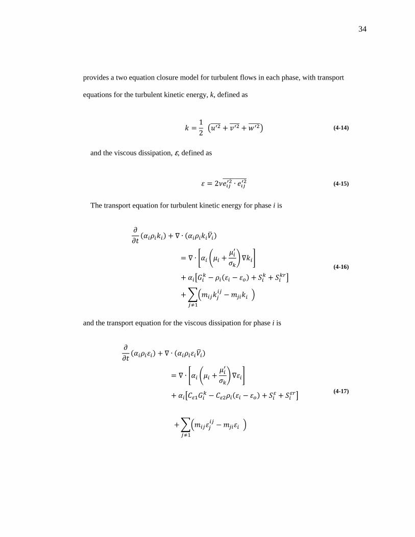
34

provides a two equation closure model for turbulent flows in each phase, with transport

equations for the turbulent kinetic energy, k, defined as

and the viscous dissipation, ε, defined as

The transport equation for turbulent kinetic energy for phase i is

GG (@<) + ∇ ∙ (@<IJ)= ∇ ∙ u@ )s + s4`v+ ∇w+ @nxv − <( − 0) + Kv + Kvyo+ Sz6### − 6#

#mF

(4-16)

and the transport equation for the viscous dissipation for phase i is

GG (@<) + ∇ ∙ (@<IJ)= ∇ ∙ u@ )s + s4`v+ ∇w+ @nT|Fxv − T|D<( − 0) + K| + K|yo + Sz6### − 6#

#mF

(4-17)

= 12 V~4DJJJJ + k4DJJJJ + 4DJJJJJW (4-14)

= 24D ∙ 4DJJJJJJJJJJ (4-15)

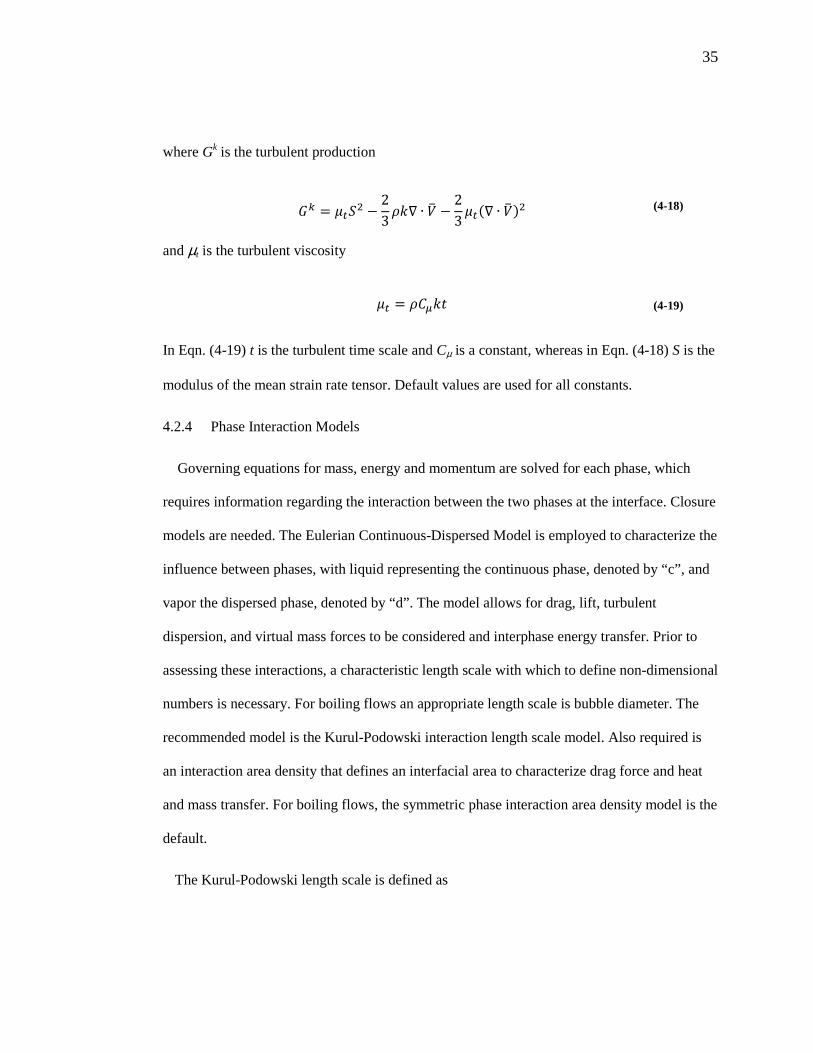
35

where Gk is the turbulent production

xv = s2KD − 23 <∇ ∙ IJ − 23 s2(∇ ∙ IJ)D (4-18)

and µt is the turbulent viscosity

s2 = <T (4-19)

In Eqn. (4-19) t is the turbulent time scale and Cµ is a constant, whereas in Eqn. (4-18) S is the

modulus of the mean strain rate tensor. Default values are used for all constants.

4.2.4 Phase Interaction Models

Governing equations for mass, energy and momentum are solved for each phase, which

requires information regarding the interaction between the two phases at the interface. Closure

models are needed. The Eulerian Continuous-Dispersed Model is employed to characterize the

influence between phases, with liquid representing the continuous phase, denoted by “c”, and

vapor the dispersed phase, denoted by “d”. The model allows for drag, lift, turbulent

dispersion, and virtual mass forces to be considered and interphase energy transfer. Prior to

assessing these interactions, a characteristic length scale with which to define non-dimensional

numbers is necessary. For boiling flows an appropriate length scale is bubble diameter. The

recommended model is the Kurul-Podowski interaction length scale model. Also required is

an interaction area density that defines an interfacial area to characterize drag force and heat

and mass transfer. For boiling flows, the symmetric phase interaction area density model is the

default.

The Kurul-Podowski length scale is defined as

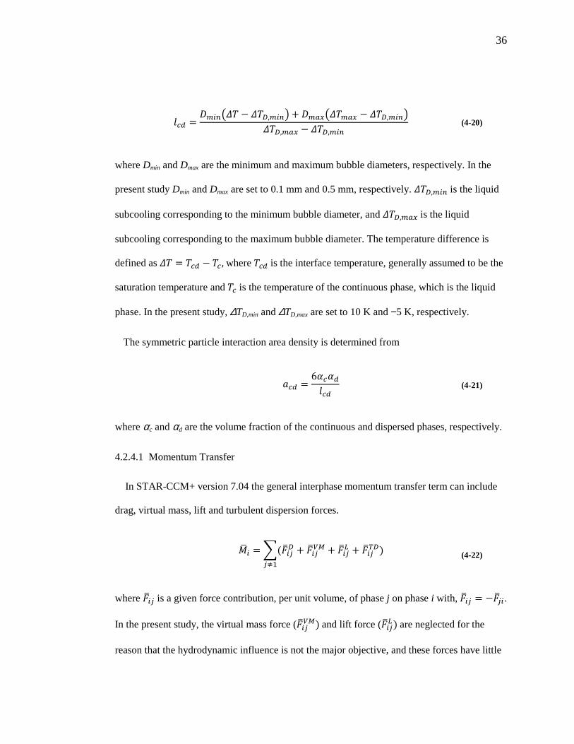
36

= 7Vi − i,7W + Vi − i,7Wi, − i,7 (4-20)

where Dmin and Dmax are the minimum and maximum bubble diameters, respectively. In the

present study Dmin and Dmax are set to 0.1 mm and 0.5 mm, respectively. i,7 is the liquid

subcooling corresponding to the minimum bubble diameter, and i, is the liquid

subcooling corresponding to the maximum bubble diameter. The temperature difference is

defined as i = − , where is the interface temperature, generally assumed to be the

saturation temperature and is the temperature of the continuous phase, which is the liquid

phase. In the present study, ∆TD,min and ∆TD,max are set to 10 K and −5 K, respectively.

The symmetric particle interaction area density is determined from

= 6@@ (4-21)

where αc and αd are the volume fraction of the continuous and dispersed phases, respectively.

4.2.4.1 Momentum Transfer

In STAR-CCM+ version 7.04 the general interphase momentum transfer term can include

drag, virtual mass, lift and turbulent dispersion forces.

pq = S(J# + J#A + J# + J#)#mF

(4-22)

where J# is a given force contribution, per unit volume, of phase j on phase i with, J# = −J#. In the present study, the virtual mass force (J#A) and lift force (J# ) are neglected for the

reason that the hydrodynamic influence is not the major objective, and these forces have little

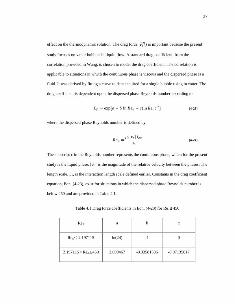
37

effect on the thermodynamic solution. The drag force (J#) is important because the present

study focuses on vapor bubbles in liquid flow. A standard drag coefficient, from the

correlation provided in Wang, is chosen to model the drag coefficient. The correlation is

applicable to situations in which the continuous phase is viscous and the dispersed phase is a

fluid. It was derived by fitting a curve to data acquired for a single bubble rising in water. The

drag coefficient is dependent upon the dispersed phase Reynolds number according to

T = exp O + + (ln ) DR (4-23)

where the dispersed-phase Reynolds number is defined by

= <|ky| μ (4-24)

The subscript c in the Reynolds number represents the continuous phase, which for the present

study is the liquid phase. |ky| is the magnitude of the relative velocity between the phases. The

length scale, lcd, is the interaction length scale defined earlier. Constants in the drag coefficient

equation, Eqn. (4-23), exist for situations in which the dispersed phase Reynolds number is

below 450 and are provided in Table 4.1.

Table 4.1 Drag force coefficients in Eqn. (4-23) for Red ≤ 450

Red a b c

Red ≤ 2.197115 ln(24) -1 0

2.197115 < Red ≤ 450 2.699467 -0.33581596 -0.07135617

38

For Red > 450, the drag coefficient is determined from

T = 38 + 4 (4-25)

instead of from Eqn. (4-23). The Eotvos number, defined as

= (< − <)M"D (4-26)

is computed from bubble diameter, or as appropriate for the Eulerian Continuous-Dispersed

Model the interaction length scale, lcd, and from water and air properties evaluated at a

temperature of 293K.

Turbulent dispersion force (J#) accounts for the interaction of the dispersed phase with

turbulent eddies in the continuous phase. It is defined by

J# = 5# k2d 2, )@#@# − @@ + (4-27)

where k2 is the turbulent kinematic viscosity of the continuous phase and d 2, is the turbulent

Prandtl number of the continuous phase, the values of which is set to 0.08 Pa-s and 0.9,

respectively, in the present study. According to the Symmetric Drag Model, which is

applicable to fluid-fluid interactions, the linearized drag coefficient is defined by

5# = 34 T@@(@< + @<)@ + @ (4-28)

where CD is found from Eqn. (4-23) in combination with constants found in Table 4.1. The

continuous and dispersed phase length scale, lc and ld, are well characterized by the interaction

length scale, lcd.

39

4.2.4.2 Energy Transfer

The heat transfer resulting from thermal diffusion from phase i to phase j is represented by

r# = −r# = ℎ(#)#(# − ) (4-29)

where aij is the interfacial area per unit volume, which is acd when using the Eulerian

Continuous-Dispersed model. Temperatures Ti and Tj are the bulk temperatures of the

continuous and dispersed phases, respectively, and ℎ(#) is the average heat transfer coefficient

at the interface, which is defined as

ℎ(#) = ~ (4-30)

The Nusselt number is determined from the Ranz-Marshall correlation

~ = 2 + 0.6,. d ,.g (4-31)

4.2.4.3 Boiling Mass Transfer

The interface mass transfer is determined from a heat balance at an interface

6(#) = r(#) + r#(#)ℎ# (4-32)

where 6(#) is the rate of mass transfer across the interface from phase i to phase j and hij

represents the enthalpy difference between phase i and phase j. The heat transfer from the

interface, at which phase change occurs, to the phases on either side of the interface is

modeled as

40

r(#) = ℎ(#)#(# − ) (4-33)

r#(#) = ℎ#(#)#(# − #) (4-34)

where

ℎ(#) = ~# (4-35)

ℎ#(#) = #~## (4-36)

The dispersed phase Nusselt number is assigned a value of 2, as the default, whereas the

continuous phase Nusselt number is computed using the Ranz-Marshall correlation in Eqn. (4-

31).

4.2.5 Boiling Model

The boiling model employed for the Multiphase Segregated Flow formulation, often

referred to as the Wall Boiling model, incorporates the subcooled boiling model from Kurul

and Podowski modified to account for heat transfer to a vapor phase. The subcooled boiling

model assumes that heat transfer from the solid surface to the liquid occurs via three different

mechanisms: convection, evaporation, and quenching. Heat transfer from the surface to the

vapor phase is by convection, and occurs to the fraction of the surface in contact with vapor,

Kdry.

344 = V307;44 + 3;U44 + 3c17¡44 WV1 − y¢W + y¢3y¢44 (4-37)

4.2.5.1 Convective Heat Transfer

The turbulent convection fluxes are

41

307;44 = <9U9~9∗9£ ( − 9) (4-38)

3y¢44 = <¤U¤~¤∗¤£ ( − ¤) (4-39)

where ~∗ and £ represent friction velocities and dimensionless temperature differences,

between the average fluid temperature and the wall temperature for the phase of interest,

inside the viscous sublayer.

Wall dryout occurs locally when the vapor volume fraction exceeds a specified value, αdry,

which for the present study is 0.9. An expression for characterizing the fraction of the wall in

contact with vapor is

y¢ = ¥ 0 @ ≤ @y¢§D(3 − 2§) @ > @y¢ (4-40)

where

§ = @¤ − @y¢1 − @y¢ (4-41)

which varies between 0 and 1.

4.2.5.2 Evaporative Heat Transfer

The heat flux due to evaporation is determined using

3;U44 = 44Z )©"g6 + <¤ℎ9¤ (4-42)

where n″ is the density of nucleation sites and dw and f are the departure diameter and

departure frequency of the bubble, respectively. The number of active nucleation sites is a

42

function of wall superheat, the critical cavity size and the three phase contact angle, and for

the present study is determined using the Hibiki and Ishii model

44 = 44JJJJ )1 − exp u− ªD8Θ Dw+ )exp uZ(< +) «4

w − 1+ (4-43)

In Eqn. (4-43), 44JJJJ represents an average cavity density, which has a default value of 4.74x105

sites/m2. The liquid-vapor contact angles, θ, were assigned room temperature values of 20°

and 127° at the heated aluminum and porous Telfon surfaces, respectively, but allowed to

change with temperature. The scale factor, Θ, for the wall contact angle is set at 20°. The

logarithmic, non-dimensional density function f(ρ+) employs default constants, and Rc and λ′

are the critical cavity radius and the length scale of the cavity. The cavity length scale was set

to a default value of 2.5x10-6 m. The critical cavity radius is determined from

= 2`(1 + (<¤<9 )/Y9)exp uℎ9¤V¤ − b2W¤b2 w − 1 (4-44)

where R is the gas constant for water vapor, 0.4615 kJ/kg-K.

The correlation developed by Kocamustafaogullari is based on a force balance between the

gravity force and surface tension force with a density correction ratio

" = "Fª ­ `Mi<®,. )i<<¤ +,.¯ (4-45)

In Eqn. (4-45), d1 is a constant having a value of 2.64x10-5 m/degree. The value of ª is set to

20° and i< is the difference in density between the liquid and gas phases.

43

The model used to compute bubble departure frequency is the Cole model, which represents

the bubble rise velocity (estimated using the drag coefficient) divided by bubble departure

diameter

Z = _34 M(<9 − <¤)"<9 (4-46)

4.2.5.3 Heat Transfer due to quenching

This component of heat flux is modeled using the relation provided by Del Valle and

Kenning.

3c17¡44 = ℎc17¡(99 − 9) (4-47)

ℎc17¡ = 2c17¡Z_<9TU99© (4-48)

where c17¡ represents the fraction of wall area subjected to quenching, which is larger

than the footprint of the bubble and is determined from the Kurul-Podowski relation

c17¡ = ©"D4 ′′ (4-49)

In Eqn. (4-43), FA is a scaling coefficient relating the area of nucleation sites and the area

subjected to bubble-induced quenching. The default value, based on recommendations by

Bartolomei and Chanturiya, is 2.0. The variable is the time between bubble departure and

nucleation of the next bubble and is given by

44

= TZ (4-50)

The coefficient T has a default value of 0.8 based on an assumption by Kurul and Podowski

that quenching occurs during 80% of the departure cycle.

4.2.6 Wall Permeability Model

A wall made permeable to a particular phase, in this case permeable to vapor, allows the

approaching vapor to leave through this boundary. The mass flux of this phase, j, is assessed

using density, velocity and volume fraction evaluated at the cell centers adjacent to the

permeable wall

6# = <#Iq ∙ 5 @# # (4-51)

where 5 is the unit normal area vector associated with the permeable wall of the cell of

interest, and # is the permeability factor of the wall, which can vary from 0 to 1. The wall

permeability factor regulates the amount of the vapor flux normal to the surface allowed to

transport through the permeable wall. The tangential component of vapor flux is zero,

corresponding to a no-slip wall boundary. The vapor flux through the wall is used in all the

other transport equations.

4.2.7 Computational Details

For all partial differential equations, a second order upwind differencing scheme was used

for the advective terms and a central differencing scheme was used for diffusive terms. An

arithmetic multi-grid V cycle solver was employed with a 50 level limit and a 30 cycle

maximum. Under relaxation factors between 0.6 and 0.2 were employed for velocity and

energy for heat flux ranges between 5 and 50 W/cm2, respectively. An under-relaxation value

45

of 0.3 was used for pressure. For stability, an initial condition of 0.01 for vapor volume

fraction was assigned to the computational domain. An under-relaxation factor of 0.1 was used

for the VOF model with a solid phase under-relaxation factor of 0.99.

46

Chapter 5 – Data Reduction and CFD Validation

Data reduction methods are presented and include average wall temperature for validation

purposes. Also presented are definitions of dimensionless gap height, temperature and

velocity, which is how profiles are presented in Chapter 6.

Results generated from Star-CCM+ for a specified base case are compared to experimental

boiling curves. A single jet diameter of 4 mm was investigated. The base case has a gap

height, Z, of 0.5 mm, a mass flux, G, of 400 kg/m2-s and a heat flux, qˮ, of 20 W/cm2. For

extraction case, a driving pressure differential, ∇p, of 20 kPa is employed. Heat flux is varied

between 0 and 50 W/cm2 to generate the boiling curves. For boiling curves, the wall superheat

is needed as a function of applied heat flux.

5.1 Data Reduction

To validate the solutions wall superheats and vapor generation are compared, respectively,

to experimental values in the form of boiling curves and to theoretical exit qualities

determined from an energy balance. The equation to assess theoretical vapor generation is

provided by Eqn. (3.1) in Chapter 3. Because wall superheat is defined as Tw – Tsat, an average

wall temperature is needed.

5.1.1 Area-averaged wall temperatures

A 10 degree slice of the single circular confined jet of radius was investigated. Figure 5.1

shows a representative slice with five area sectors. Wall temperature data exist at the center of

each cell face adjacent to the wall, not at the center of each sector as shown in Figure 5.1. To

achieve a radial distribution of wall temperature, a series of n radial sensors were located to

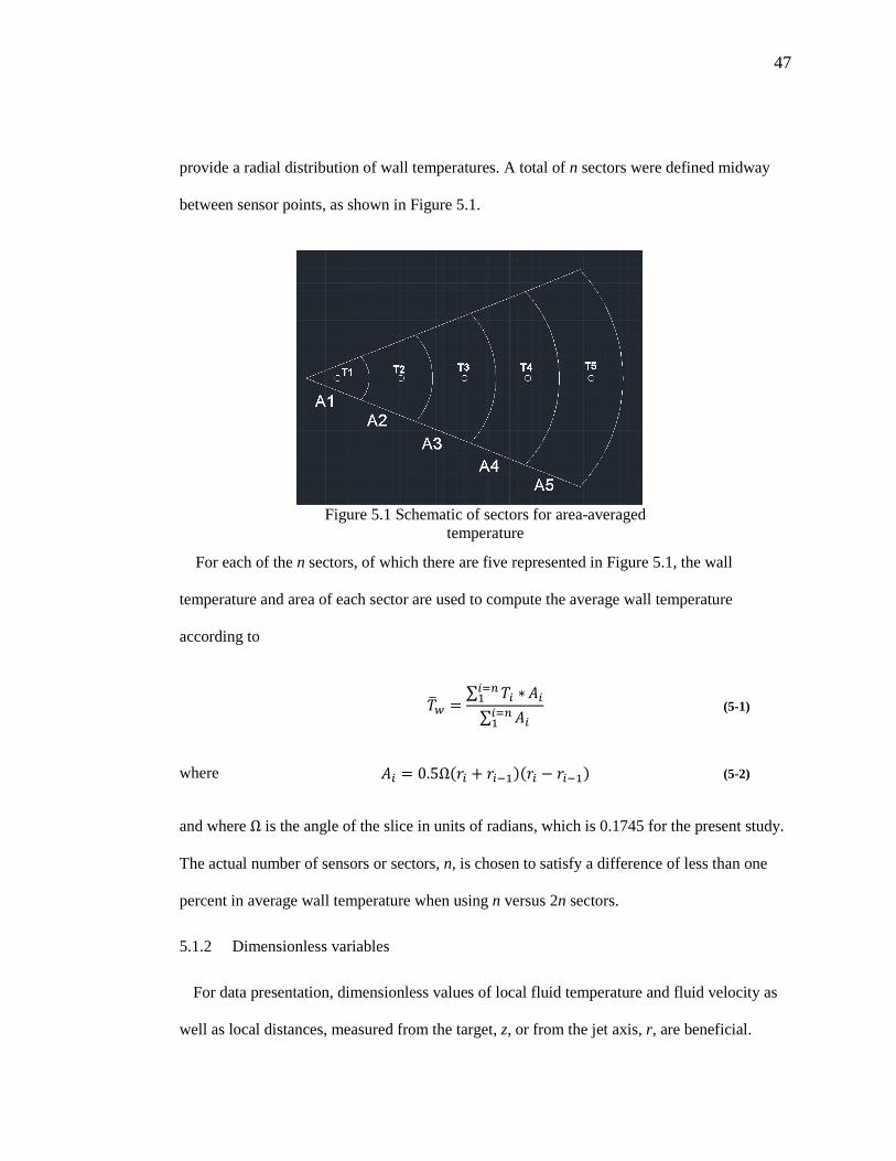
47

provide a radial distribution of wall temperatures. A total of n sectors were defined midway

between sensor points, as shown in Figure 5.1.

Figure 5.1 Schematic of sectors for area-averaged temperature

For each of the n sectors, of which there are five represented in Figure 5.1, the wall

temperature and area of each sector are used to compute the average wall temperature

according to

J = ∑ ∗E7F 5∑ 5E7F (5-1)

where 5 = 0.5Ω( + ¶F)( − ¶F) (5-2)

and where Ω is the angle of the slice in units of radians, which is 0.1745 for the present study.

The actual number of sensors or sectors, n, is chosen to satisfy a difference of less than one

percent in average wall temperature when using n versus 2n sectors.

5.1.2 Dimensionless variables

For data presentation, dimensionless values of local fluid temperature and fluid velocity as

well as local distances, measured from the target, z, or from the jet axis, r, are beneficial.

48

Local fluid temperatures, T, are made dimensionless by subtracting the saturation temperature,

based on the jet inlet pressure, and by using a reference temperature based on heat flux.

∗ = − b2y (5-3)

where y = 3"· (5-4)

In Equation (5-4), K is the thermal conductivity of the fluid, held constant in the present study,

and Z is the gap height. Local fluid velocities, v, are normalized by the jet velocity, vj, where v

can represent either the radial velocity, vr, or transverse, vz, velocity.

k∗ = kk# (5-5)

The local radial location, r, is scaled by the jet radius, r j, and the distance from the target, z, is

scaled by the gap height, Z.

∗ = # (5-6)

¸∗ = · (5-7)

5.2 Residual and grid refinement convergence

A heat flux was supplied to the bottom of the aluminum heater block and a steady state

condition was considered achieved when the energy leaving the block and entering the fluid

was within 0.01% of that applied at the bottom of the block. For each test case, the solution

was converged in terms of the grid size and residual tolerance. Three grid sizes were

considered. After some preliminary investigations a medium grid size consisting of

approximately 350,000 cells was employed for the base case. A coarser grid with 50% fewer

49

cells in each direction (cells twice as large in each direction) and a finer grid with 50% more

cells were assessed. The differences in wall surface temperature for the medium and fine grids

were 2.5K and 1.2K, respectively. A solution was considered residual-converged when most

of the residuals fell below 0.001. Refer to Appendice A.

5.3 Turbulent kinetic energy and dissipation

As reported by Zuckerman and Lior [8], use of the standard k-ε model in jet flows can yield

inadequate results. However, the highest jet Reynolds is 2,500 and the lowest dimensionless

gap spacing, Z/dj is 0.5. For flow to exceed this Reynolds number, the dimensionless gap

height must be less than 0.25. The lowest gap height tested results in a dimensionless gap

height of 0.5; therefore, the liquid in its subcooled state never reaches a turbulent state.

Furthermore, given the increase in area with r, even as the flow becomes two-phase, it will

likely remain laminar.

A laminar flow analysis was conducted using the VOF model whereas the MSF wall boiling

model required a turbulent flow analysis. However, if the turbulent kinetic energy and viscous

dissipation approach zero, they have little impact on the solution and should therefore not

yield inadequate results. For the base case, the average k and ε were 8.8x10-11and 6.6x10-10,

respectively.

5.4 Validation

To validate the results, simulations of exit quality and wall superheats are compared to

theory and experiments, respectively, in Figure 5.2 and Figure 5.3. Simulations for the base

case using both VOF and MSF models are provided.

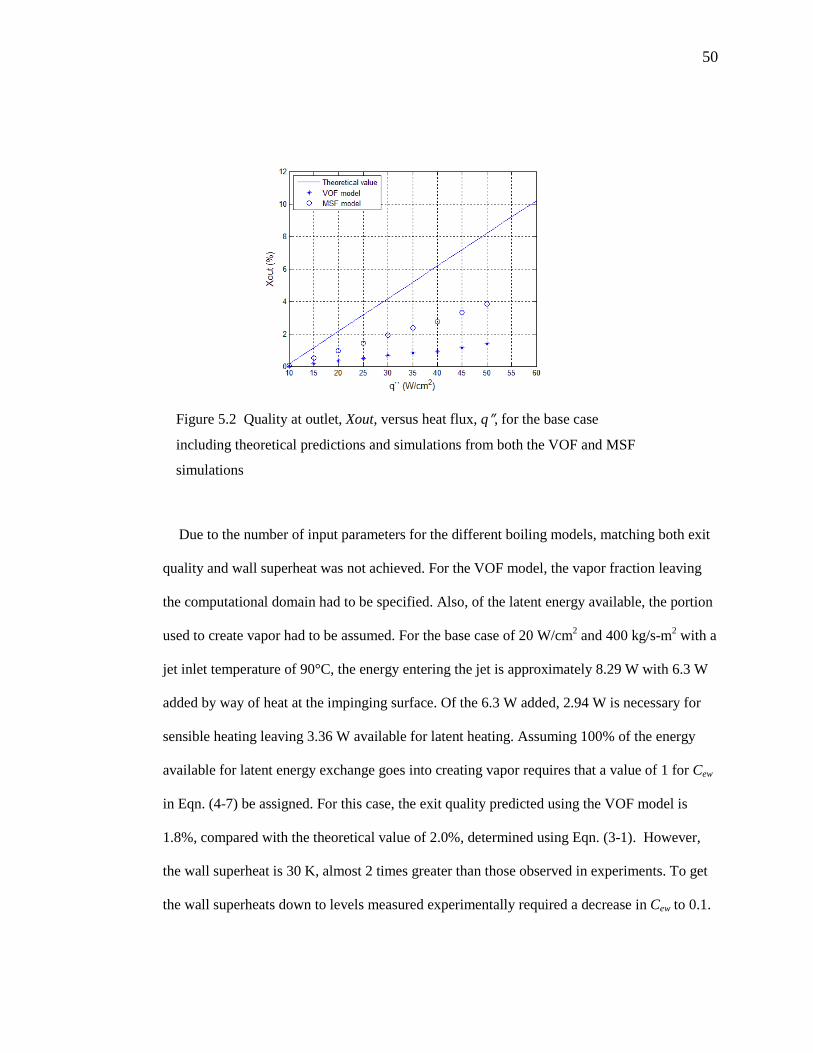
50

Due to the number of input parameters for the different boiling models, matching both exit

quality and wall superheat was not achieved. For the VOF model, the vapor fraction leaving

the computational domain had to be specified. Also, of the latent energy available, the portion

used to create vapor had to be assumed. For the base case of 20 W/cm2 and 400 kg/s-m2 with a

jet inlet temperature of 90°C, the energy entering the jet is approximately 8.29 W with 6.3 W

added by way of heat at the impinging surface. Of the 6.3 W added, 2.94 W is necessary for

sensible heating leaving 3.36 W available for latent heating. Assuming 100% of the energy

available for latent energy exchange goes into creating vapor requires that a value of 1 for Cew

in Eqn. (4-7) be assigned. For this case, the exit quality predicted using the VOF model is

1.8%, compared with the theoretical value of 2.0%, determined using Eqn. (3-1). However,

the wall superheat is 30 K, almost 2 times greater than those observed in experiments. To get

the wall superheats down to levels measured experimentally required a decrease in Cew to 0.1.

Figure 5.2 Quality at outlet, Xout, versus heat flux, q″, for the base case

including theoretical predictions and simulations from both the VOF and MSF

simulations

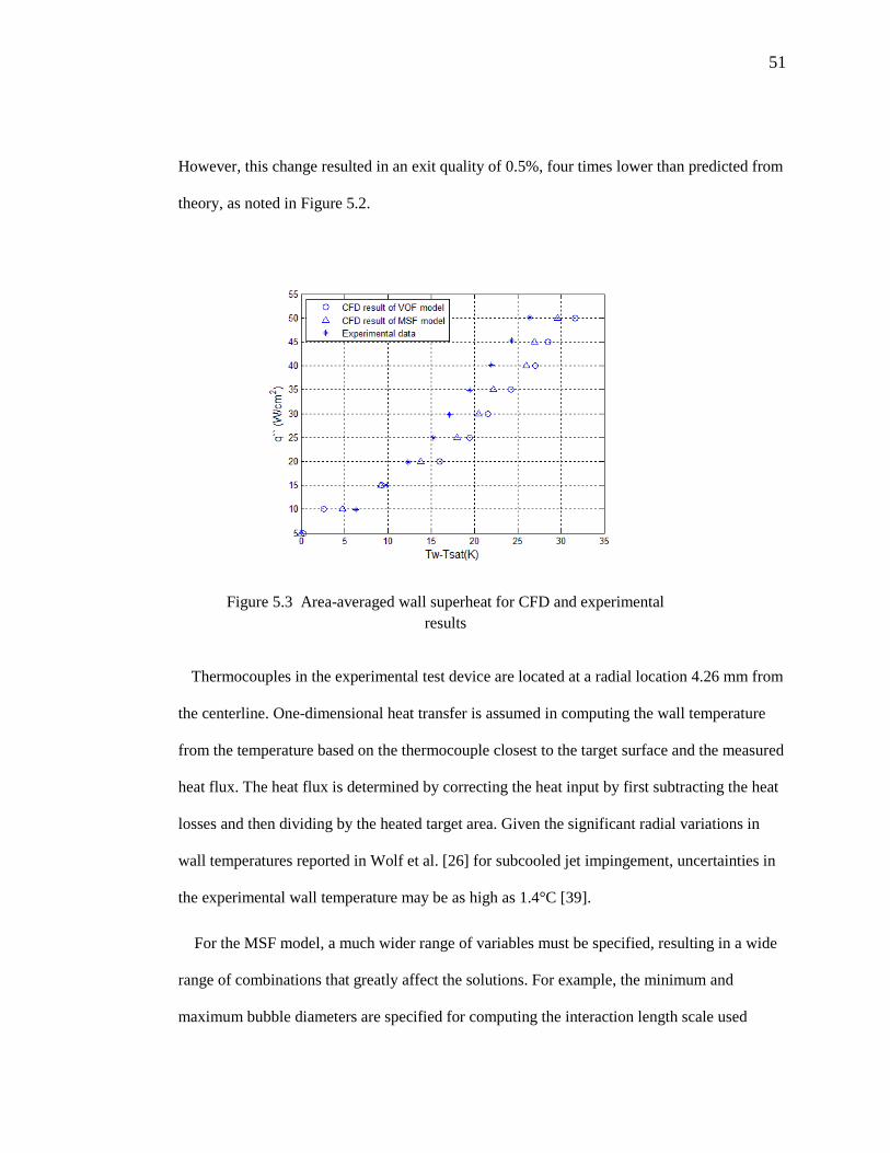
51

However, this change resulted in an exit quality of 0.5%, four times lower than predicted from

theory, as noted in Figure 5.2.

Thermocouples in the experimental test device are located at a radial location 4.26 mm from

the centerline. One-dimensional heat transfer is assumed in computing the wall temperature

from the temperature based on the thermocouple closest to the target surface and the measured

heat flux. The heat flux is determined by correcting the heat input by first subtracting the heat

losses and then dividing by the heated target area. Given the significant radial variations in

wall temperatures reported in Wolf et al. [26] for subcooled jet impingement, uncertainties in

the experimental wall temperature may be as high as 1.4°C [39].

For the MSF model, a much wider range of variables must be specified, resulting in a wide

range of combinations that greatly affect the solutions. For example, the minimum and

maximum bubble diameters are specified for computing the interaction length scale used

Figure 5.3 Area-averaged wall superheat for CFD and experimental results

52

throughout the analysis. Also specified is a wall dry out factor and a scale factor for the

contact angle in the equation used to assess average cavity density. To select the correct

parameters and to validate this model requires more comprehensive experimental

measurements, preferably local wall temperatures.

Because the VOF model has the more reasonable method for extracting vapor and because

it can achieve local wall temperatures close to those achieved experimentally, simulations

were run with Cew near 10% and are presented in the following chapter. Results of exit quality

and wall superheat in Figure 5.2 and Figure 5.3, respectively, are for this value of Cew and the

range of input parameters for the MSF model are specified in Appendice B.

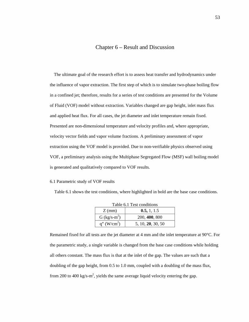
53

Chapter 6 – Result and Discussion

The ultimate goal of the research effort is to assess heat transfer and hydrodynamics under

the influence of vapor extraction. The first step of which is to simulate two-phase boiling flow

in a confined jet; therefore, results for a series of test conditions are presented for the Volume

of Fluid (VOF) model without extraction. Variables changed are gap height, inlet mass flux

and applied heat flux. For all cases, the jet diameter and inlet temperature remain fixed.

Presented are non-dimensional temperature and velocity profiles and, where appropriate,

velocity vector fields and vapor volume fractions. A preliminary assessment of vapor

extraction using the VOF model is provided. Due to non-verifiable physics observed using

VOF, a preliminary analysis using the Multiphase Segregated Flow (MSF) wall boiling model

is generated and qualitatively compared to VOF results.

6.1 Parametric study of VOF results

Table 6.1 shows the test conditions, where highlighted in bold are the base case conditions.

Table 6.1 Test conditions Z (mm) 0.5, 1, 1.5

G (kg/s-m2) 200, 400, 800

qˮ (W/cm2) 5, 10, 20, 30, 50

Remained fixed for all tests are the jet diameter at 4 mm and the inlet temperature at 90°C. For

the parametric study, a single variable is changed from the base case conditions while holding

all others constant. The mass flux is that at the inlet of the gap. The values are such that a

doubling of the gap height, from 0.5 to 1.0 mm, coupled with a doubling of the mass flux,

from 200 to 400 kg/s-m2, yields the same average liquid velocity entering the gap.

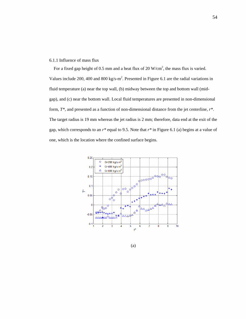
54

6.1.1 Influence of mass flux

For a fixed gap height of 0.5 mm and a heat flux of 20 W/cm2, the mass flux is varied.

Values include 200, 400 and 800 kg/s-m2. Presented in Figure 6.1 are the radial variations in

fluid temperature (a) near the top wall, (b) midway between the top and bottom wall (mid-

gap), and (c) near the bottom wall. Local fluid temperatures are presented in non-dimensional

form, T*, and presented as a function of non-dimensional distance from the jet centerline, r* .

The target radius is 19 mm whereas the jet radius is 2 mm; therefore, data end at the exit of the

gap, which corresponds to an r* equal to 9.5. Note that r* in Figure 6.1 (a) begins at a value of

one, which is the location where the confined surface begins.

(a)

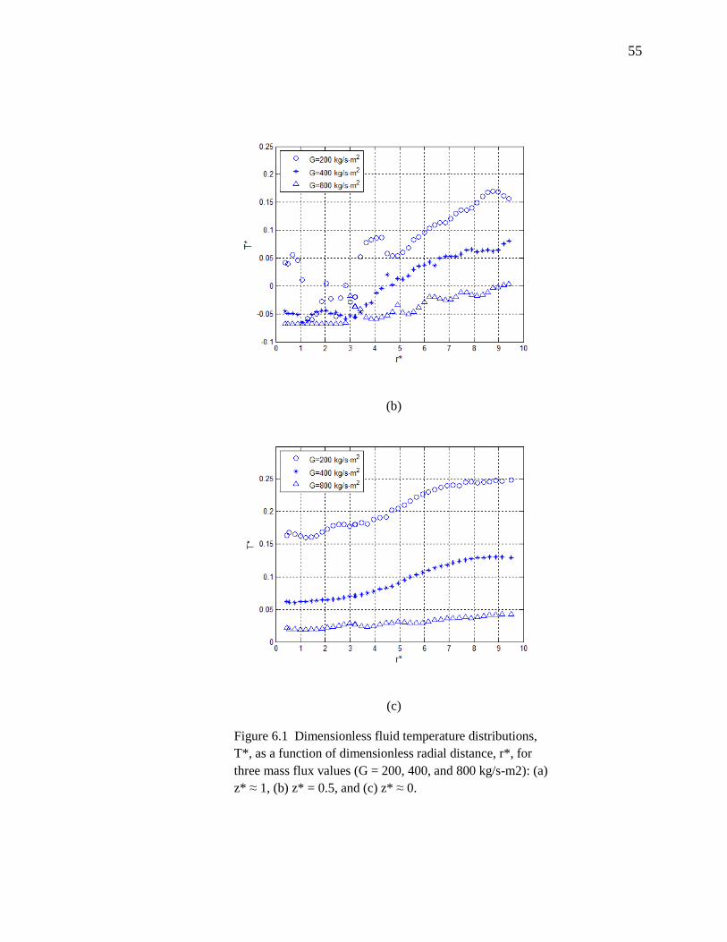
55

(b)

(c)

Figure 6.1 Dimensionless fluid temperature distributions, T*, as a function of dimensionless radial distance, r*, for three mass flux values (G = 200, 400, and 800 kg/s-m2): (a) z* ≈ 1, (b) z* = 0.5, and (c) z* ≈ 0.

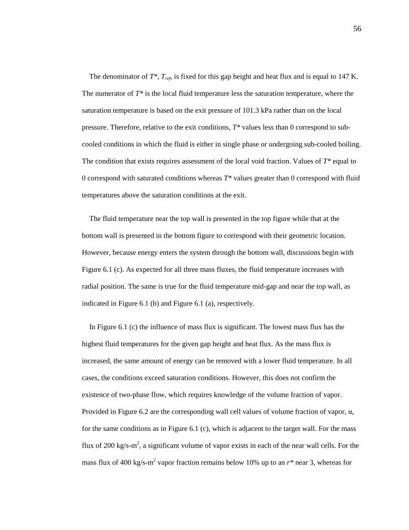
56

The denominator of T*, Tref, is fixed for this gap height and heat flux and is equal to 147 K.

The numerator of T* is the local fluid temperature less the saturation temperature, where the

saturation temperature is based on the exit pressure of 101.3 kPa rather than on the local

pressure. Therefore, relative to the exit conditions, T* values less than 0 correspond to sub-

cooled conditions in which the fluid is either in single phase or undergoing sub-cooled boiling.

The condition that exists requires assessment of the local void fraction. Values of T* equal to

0 correspond with saturated conditions whereas T* values greater than 0 correspond with fluid

temperatures above the saturation conditions at the exit.

The fluid temperature near the top wall is presented in the top figure while that at the

bottom wall is presented in the bottom figure to correspond with their geometric location.

However, because energy enters the system through the bottom wall, discussions begin with

Figure 6.1 (c). As expected for all three mass fluxes, the fluid temperature increases with

radial position. The same is true for the fluid temperature mid-gap and near the top wall, as

indicated in Figure 6.1 (b) and Figure 6.1 (a), respectively.

In Figure 6.1 (c) the influence of mass flux is significant. The lowest mass flux has the

highest fluid temperatures for the given gap height and heat flux. As the mass flux is

increased, the same amount of energy can be removed with a lower fluid temperature. In all

cases, the conditions exceed saturation conditions. However, this does not confirm the

existence of two-phase flow, which requires knowledge of the volume fraction of vapor.

Provided in Figure 6.2 are the corresponding wall cell values of volume fraction of vapor, α,

for the same conditions as in Figure 6.1 (c), which is adjacent to the target wall. For the mass

flux of 200 kg/s-m2, a significant volume of vapor exists in each of the near wall cells. For the

mass flux of 400 kg/s-m2 vapor fraction remains below 10% up to an r* near 3, whereas for

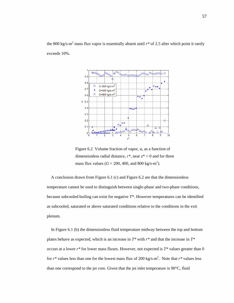
57

the 800 kg/s-m2 mass flux vapor is essentially absent until r* of 2.5 after which point it rarely

exceeds 10%.

Figure 6.2 Volume fraction of vapor, α, as a function of

dimensionless radial distance, r* , near z* ≈ 0 and for three

mass flux values (G = 200, 400, and 800 kg/s-m2).

A conclusion drawn from Figure 6.1 (c) and Figure 6.2 are that the dimensionless

temperature cannot be used to distinguish between single-phase and two-phase conditions,

because subcooled boiling can exist for negative T*. However temperatures can be identified

as subcooled, saturated or above saturated conditions relative to the conditions in the exit

plenum.

In Figure 6.1 (b) the dimensionless fluid temperature midway between the top and bottom

plates behave as expected, which is an increase in T* with r* and that the increase in T*

occurs at a lower r* for lower mass fluxes. However, not expected is T* values greater than 0

for r* values less than one for the lowest mass flux of 200 kg/s-m2. Note that r* values less

than one correspond to the jet core. Given that the jet inlet temperature is 90°C, fluid

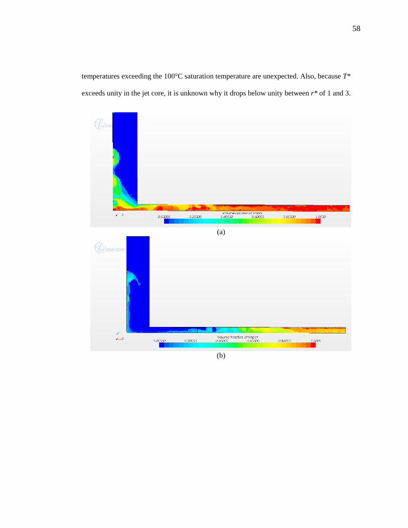
58

temperatures exceeding the 100°C saturation temperature are unexpected. Also, because T*

exceeds unity in the jet core, it is unknown why it drops below unity between r* of 1 and 3.

(a)

(b)

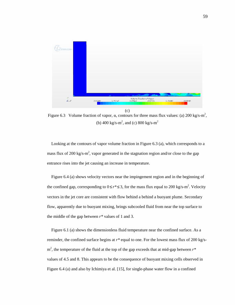
59

(c)

Figure 6.3 Volume fraction of vapor, α, contours for three mass flux values: (a) 200 kg/s-m2,

(b) 400 kg/s-m2, and (c) 800 kg/s-m2

Looking at the contours of vapor volume fraction in Figure 6.3 (a), which corresponds to a

mass flux of 200 kg/s-m2, vapor generated in the stagnation region and/or close to the gap

entrance rises into the jet causing an increase in temperature.

Figure 6.4 (a) shows velocity vectors near the impingement region and in the beginning of

the confined gap, corresponding to 0 ≤ r* ≤ 3, for the mass flux equal to 200 kg/s-m2. Velocity

vectors in the jet core are consistent with flow behind a behind a buoyant plume. Secondary

flow, apparently due to buoyant mixing, brings subcooled fluid from near the top surface to

the middle of the gap between r* values of 1 and 3.

Figure 6.1 (a) shows the dimensionless fluid temperature near the confined surface. As a

reminder, the confined surface begins at r* equal to one. For the lowest mass flux of 200 kg/s-

m2, the temperature of the fluid at the top of the gap exceeds that at mid-gap between r*

values of 4.5 and 8. This appears to be the consequence of buoyant mixing cells observed in

Figure 6.4 (a) and also by Ichimiya et al. [15], for single-phase water flow in a confined

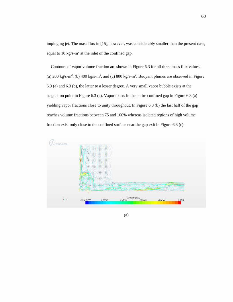
60

impinging jet. The mass flux in [15], however, was considerably smaller than the present case,

equal to 10 kg/s-m2 at the inlet of the confined gap.

Contours of vapor volume fraction are shown in Figure 6.3 for all three mass flux values:

(a) 200 kg/s-m2, (b) 400 kg/s-m2, and (c) 800 kg/s-m2. Buoyant plumes are observed in Figure

6.3 (a) and 6.3 (b), the latter to a lesser degree. A very small vapor bubble exists at the

stagnation point in Figure 6.3 (c). Vapor exists in the entire confined gap in Figure 6.3 (a)

yielding vapor fractions close to unity throughout. In Figure 6.3 (b) the last half of the gap

reaches volume fractions between 75 and 100% whereas isolated regions of high volume

fraction exist only close to the confined surface near the gap exit in Figure 6.3 (c).

(a)

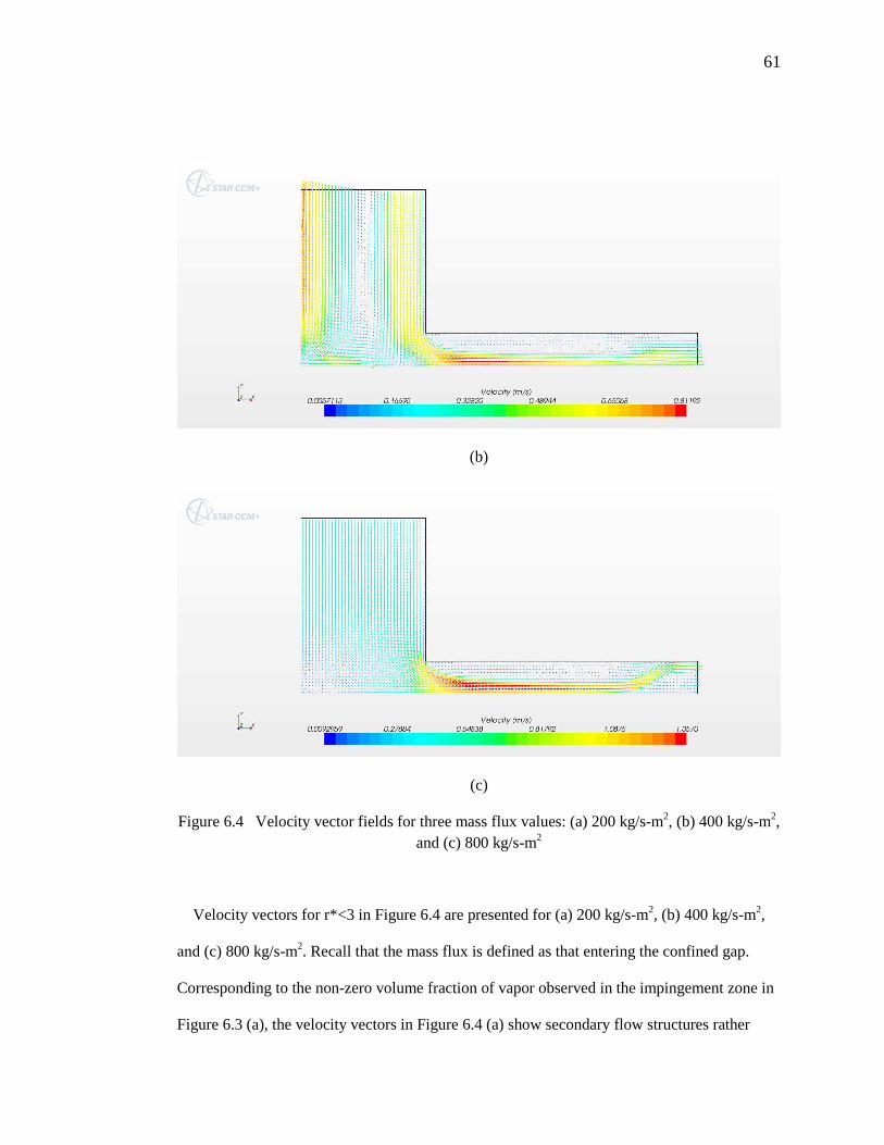
61

(b)

(c)

Figure 6.4 Velocity vector fields for three mass flux values: (a) 200 kg/s-m2, (b) 400 kg/s-m2, and (c) 800 kg/s-m2

Velocity vectors for r*<3 in Figure 6.4 are presented for (a) 200 kg/s-m2, (b) 400 kg/s-m2,

and (c) 800 kg/s-m2. Recall that the mass flux is defined as that entering the confined gap.

Corresponding to the non-zero volume fraction of vapor observed in the impingement zone in

Figure 6.3 (a), the velocity vectors in Figure 6.4 (a) show secondary flow structures rather

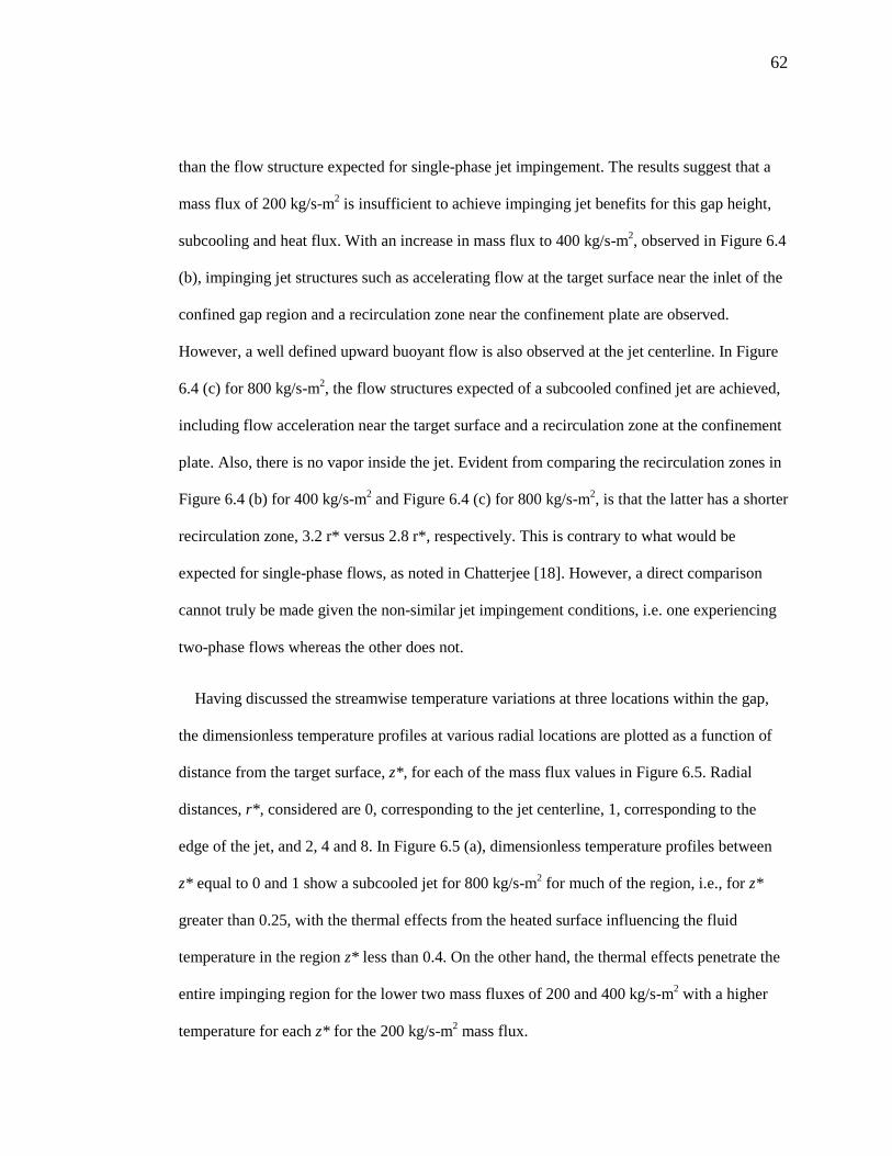
62

than the flow structure expected for single-phase jet impingement. The results suggest that a

mass flux of 200 kg/s-m2 is insufficient to achieve impinging jet benefits for this gap height,

subcooling and heat flux. With an increase in mass flux to 400 kg/s-m2, observed in Figure 6.4

(b), impinging jet structures such as accelerating flow at the target surface near the inlet of the

confined gap region and a recirculation zone near the confinement plate are observed.

However, a well defined upward buoyant flow is also observed at the jet centerline. In Figure

6.4 (c) for 800 kg/s-m2, the flow structures expected of a subcooled confined jet are achieved,

including flow acceleration near the target surface and a recirculation zone at the confinement

plate. Also, there is no vapor inside the jet. Evident from comparing the recirculation zones in

Figure 6.4 (b) for 400 kg/s-m2 and Figure 6.4 (c) for 800 kg/s-m2, is that the latter has a shorter

recirculation zone, 3.2 r* versus 2.8 r*, respectively. This is contrary to what would be

expected for single-phase flows, as noted in Chatterjee [18]. However, a direct comparison

cannot truly be made given the non-similar jet impingement conditions, i.e. one experiencing

two-phase flows whereas the other does not.

Having discussed the streamwise temperature variations at three locations within the gap,

the dimensionless temperature profiles at various radial locations are plotted as a function of

distance from the target surface, z*, for each of the mass flux values in Figure 6.5. Radial

distances, r* , considered are 0, corresponding to the jet centerline, 1, corresponding to the

edge of the jet, and 2, 4 and 8. In Figure 6.5 (a), dimensionless temperature profiles between

z* equal to 0 and 1 show a subcooled jet for 800 kg/s-m2 for much of the region, i.e., for z*

greater than 0.25, with the thermal effects from the heated surface influencing the fluid

temperature in the region z* less than 0.4. On the other hand, the thermal effects penetrate the

entire impinging region for the lower two mass fluxes of 200 and 400 kg/s-m2 with a higher

temperature for each z* for the 200 kg/s-m2 mass flux.

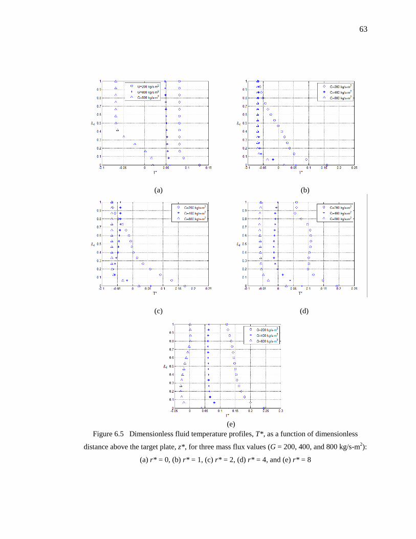
63

(a) (b)

(c) (d)

(e) Figure 6.5 Dimensionless fluid temperature profiles, T*, as a function of dimensionless

distance above the target plate, z*, for three mass flux values (G = 200, 400, and 800 kg/s-m2):

(a) r* = 0, (b) r* = 1, (c) r* = 2, (d) r* = 4, and (e) r* = 8

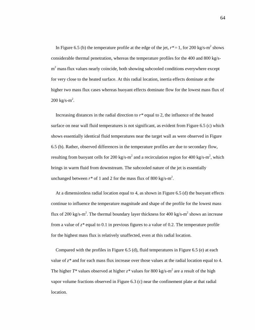
64

In Figure 6.5 (b) the temperature profile at the edge of the jet, r* = 1, for 200 kg/s-m2 shows

considerable thermal penetration, whereas the temperature profiles for the 400 and 800 kg/s-

m2 mass flux values nearly coincide, both showing subcooled conditions everywhere except

for very close to the heated surface. At this radial location, inertia effects dominate at the

higher two mass flux cases whereas buoyant effects dominate flow for the lowest mass flux of

200 kg/s-m2.

Increasing distances in the radial direction to r* equal to 2, the influence of the heated

surface on near wall fluid temperatures is not significant, as evident from Figure 6.5 (c) which

shows essentially identical fluid temperatures near the target wall as were observed in Figure

6.5 (b). Rather, observed differences in the temperature profiles are due to secondary flow,

resulting from buoyant cells for 200 kg/s-m2 and a recirculation region for 400 kg/s-m2, which

brings in warm fluid from downstream. The subcooled nature of the jet is essentially

unchanged between r* of 1 and 2 for the mass flux of 800 kg/s-m2.

At a dimensionless radial location equal to 4, as shown in Figure 6.5 (d) the buoyant effects

continue to influence the temperature magnitude and shape of the profile for the lowest mass

flux of 200 kg/s-m2. The thermal boundary layer thickness for 400 kg/s-m2 shows an increase

from a value of z* equal to 0.1 in previous figures to a value of 0.2. The temperature profile

for the highest mass flux is relatively unaffected, even at this radial location.

Compared with the profiles in Figure 6.5 (d), fluid temperatures in Figure 6.5 (e) at each

value of z* and for each mass flux increase over those values at the radial location equal to 4.

The higher T* values observed at higher z* values for 800 kg/s-m2 are a result of the high

vapor volume fractions observed in Figure 6.3 (c) near the confinement plate at that radial

location.

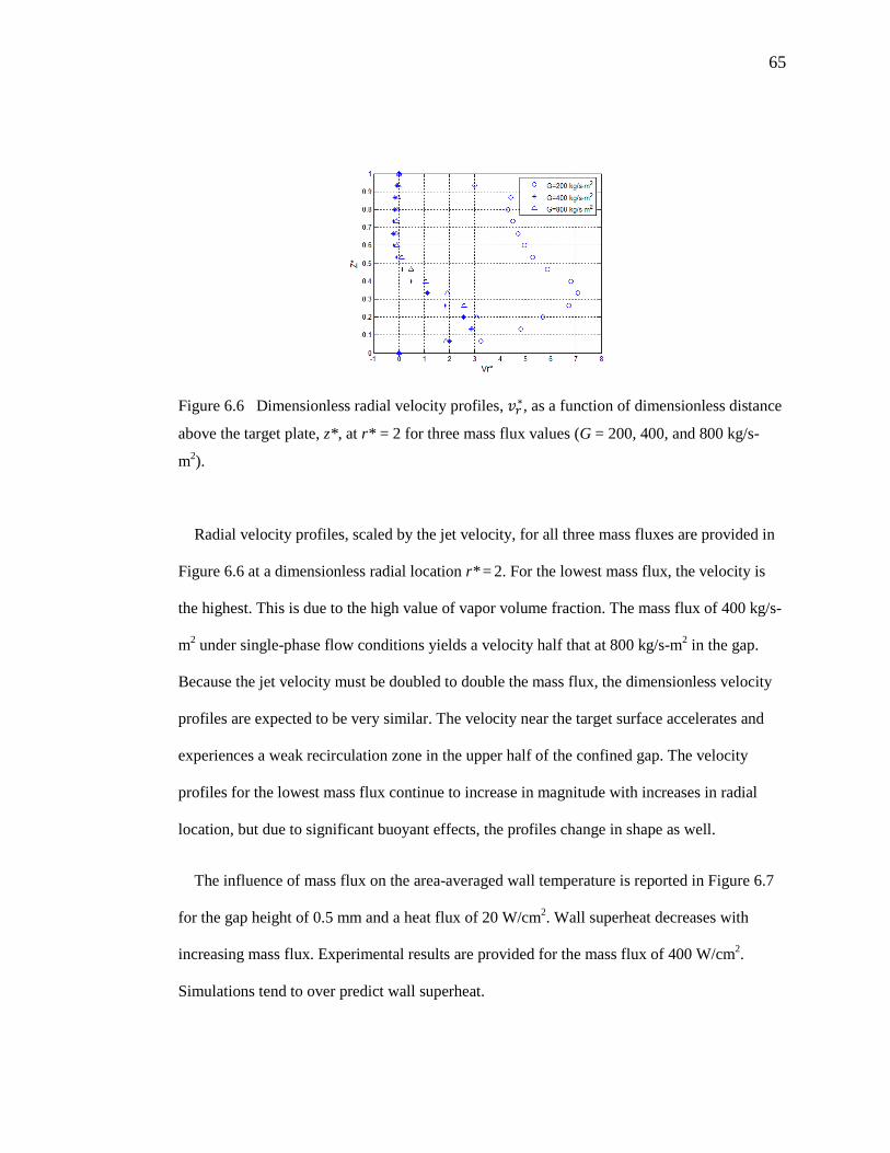
65

Figure 6.6 Dimensionless radial velocity profiles, ky∗, as a function of dimensionless distance

above the target plate, z*, at r* = 2 for three mass flux values (G = 200, 400, and 800 kg/s-

m2).

Radial velocity profiles, scaled by the jet velocity, for all three mass fluxes are provided in

Figure 6.6 at a dimensionless radial location r* = 2. For the lowest mass flux, the velocity is

the highest. This is due to the high value of vapor volume fraction. The mass flux of 400 kg/s-

m2 under single-phase flow conditions yields a velocity half that at 800 kg/s-m2 in the gap.

Because the jet velocity must be doubled to double the mass flux, the dimensionless velocity

profiles are expected to be very similar. The velocity near the target surface accelerates and

experiences a weak recirculation zone in the upper half of the confined gap. The velocity

profiles for the lowest mass flux continue to increase in magnitude with increases in radial

location, but due to significant buoyant effects, the profiles change in shape as well.

The influence of mass flux on the area-averaged wall temperature is reported in Figure 6.7

for the gap height of 0.5 mm and a heat flux of 20 W/cm2. Wall superheat decreases with

increasing mass flux. Experimental results are provided for the mass flux of 400 W/cm2.

Simulations tend to over predict wall superheat.

66

6.1.2 Influence of heat flux

Streamwise variations in dimensionless fluid temperature are shown in Figure 6.8 for five

heat flux values: 5, 10, 20, 30 and 50 W/cm2. The jet diameter, inlet jet temperature, mass flux

entering the confined gap and gap height are fixed at 4 mm, 90°C, 400 kg/s-m2, and 0.5 mm,

respectively. Fluid temperatures are shown at the top of the confined gap in Figure 6.8 (a), at

the mid-plane between the bottom and top walls in Figure 6.8 (b), and at the bottom wall in

Figure 6.8 (c).

For the conditions provided in Figure 6.8, Tref is 36.8, 73.5, 147, 221, and 367 K,

respectively, for heat flux values of 5, 10, 20, 30 and 50 W/cm2. In Figure 6.8 (c), significant

variations in fluid temperature near the target surface exist, which are indicative of changes in

Figure 6.7 Average wall superheat, − b2, as a function of mass flux, G

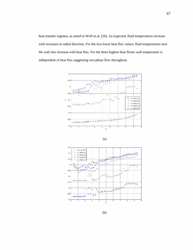
67

heat transfer regimes, as noted in Wolf et al. [26]. As expected, fluid temperatures increase

with increases in radial direction. For the two lower heat flux values, fluid temperatures near

the wall also increase with heat flux. For the three highest heat fluxes wall temperature is

independent of heat flux suggesting two-phase flow throughout.

(a)

(b)

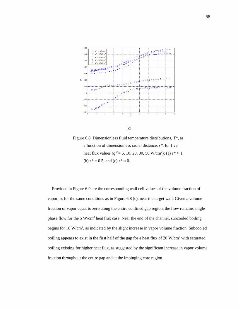
68

(c)

Figure 6.8 Dimensionless fluid temperature distributions, T*, as

a function of dimensionless radial distance, r* , for five

heat flux values (q″ = 5, 10, 20, 30, 50 W/cm2): (a) z* ≈ 1,

(b) z* = 0.5, and (c) z* ≈ 0.

Provided in Figure 6.9 are the corresponding wall cell values of the volume fraction of

vapor, α, for the same conditions as in Figure 6.8 (c), near the target wall. Given a volume

fraction of vapor equal to zero along the entire confined gap region, the flow remains single-

phase flow for the 5 W/cm2 heat flux case. Near the end of the channel, subcooled boiling

begins for 10 W/cm2, as indicated by the slight increase in vapor volume fraction. Subcooled

boiling appears to exist in the first half of the gap for a heat flux of 20 W/cm2 with saturated

boiling existing for higher heat flux, as suggested by the significant increase in vapor volume

fraction throughout the entire gap and at the impinging core region.

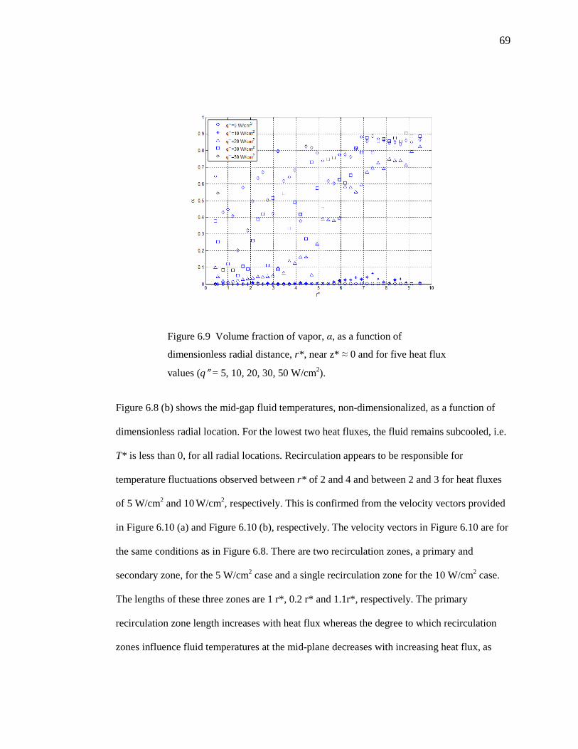
69

Figure 6.9 Volume fraction of vapor, α, as a function of

dimensionless radial distance, r* , near z* ≈ 0 and for five heat flux

values (q″ = 5, 10, 20, 30, 50 W/cm2).

Figure 6.8 (b) shows the mid-gap fluid temperatures, non-dimensionalized, as a function of

dimensionless radial location. For the lowest two heat fluxes, the fluid remains subcooled, i.e.

T* is less than 0, for all radial locations. Recirculation appears to be responsible for

temperature fluctuations observed between r* of 2 and 4 and between 2 and 3 for heat fluxes

of 5 W/cm2 and 10 W/cm2, respectively. This is confirmed from the velocity vectors provided

in Figure 6.10 (a) and Figure 6.10 (b), respectively. The velocity vectors in Figure 6.10 are for

the same conditions as in Figure 6.8. There are two recirculation zones, a primary and

secondary zone, for the 5 W/cm2 case and a single recirculation zone for the 10 W/cm2 case.

The lengths of these three zones are 1 r*, 0.2 r* and 1.1r*, respectively. The primary

recirculation zone length increases with heat flux whereas the degree to which recirculation

zones influence fluid temperatures at the mid-plane decreases with increasing heat flux, as

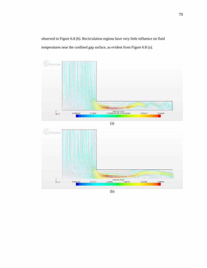
70

observed in Figure 6.8 (b). Recirculation regions have very little influence on fluid

temperatures near the confined gap surface, as evident from Figure 6.8 (a).

(a)

(b)

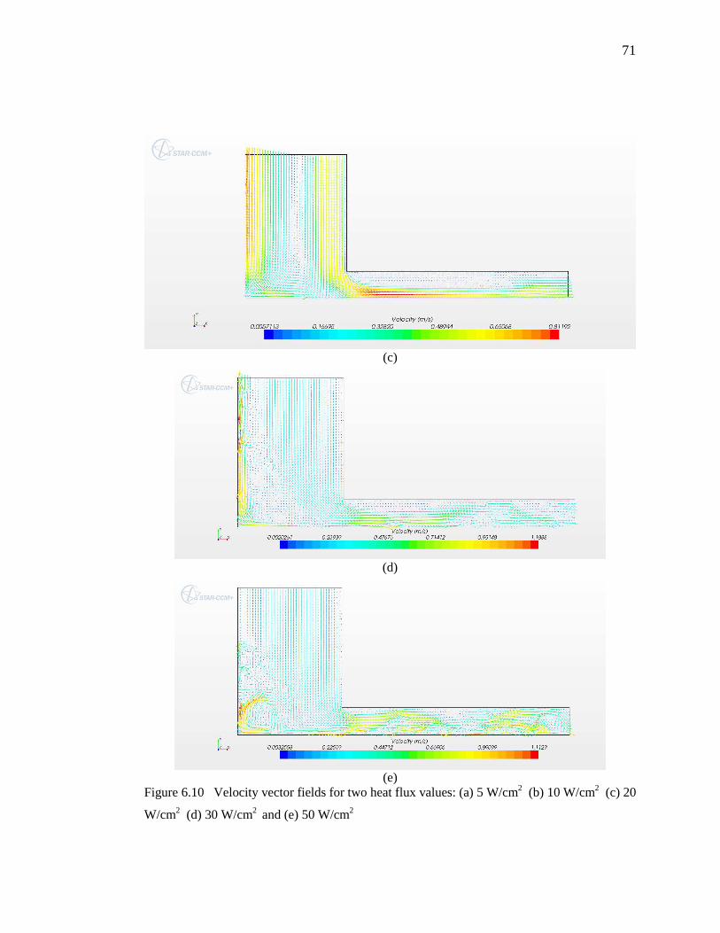
71

(c)

(d)

(e)

Figure 6.10 Velocity vector fields for two heat flux values: (a) 5 W/cm2 (b) 10 W/cm2 (c) 20

W/cm2 (d) 30 W/cm2 and (e) 50 W/cm2

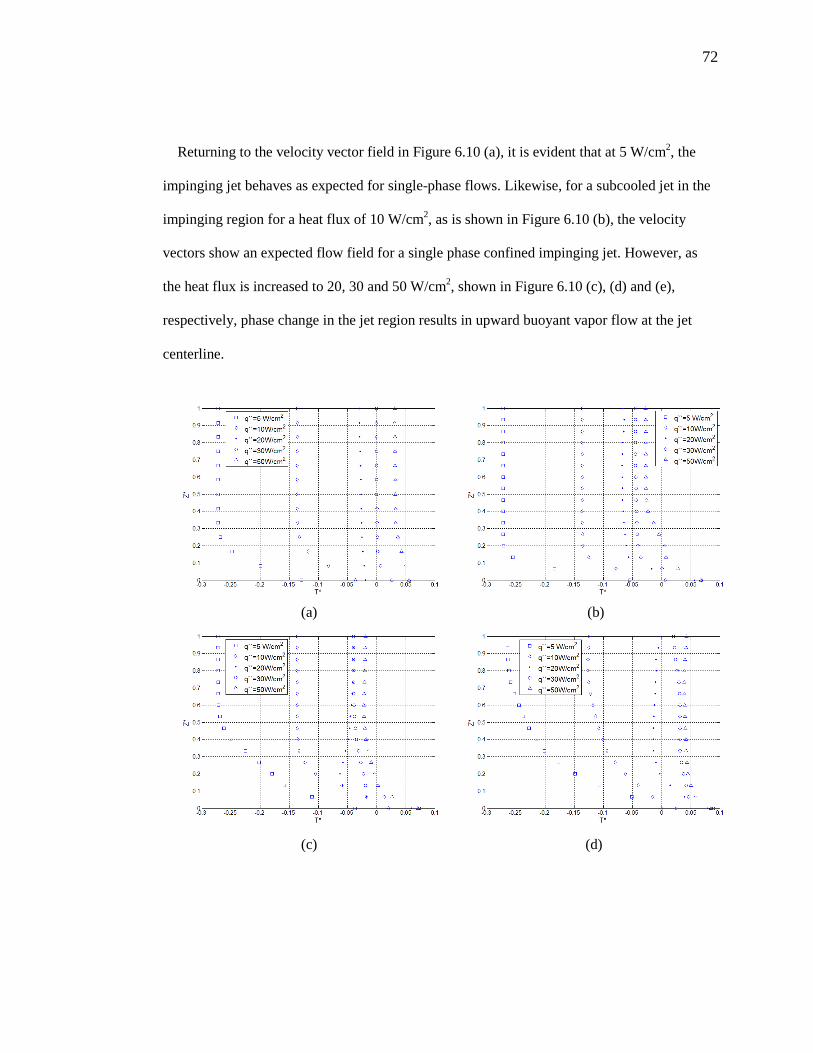
72

Returning to the velocity vector field in Figure 6.10 (a), it is evident that at 5 W/cm2, the

impinging jet behaves as expected for single-phase flows. Likewise, for a subcooled jet in the

impinging region for a heat flux of 10 W/cm2, as is shown in Figure 6.10 (b), the velocity

vectors show an expected flow field for a single phase confined impinging jet. However, as

the heat flux is increased to 20, 30 and 50 W/cm2, shown in Figure 6.10 (c), (d) and (e),

respectively, phase change in the jet region results in upward buoyant vapor flow at the jet

centerline.

(a) (b)

(c) (d)

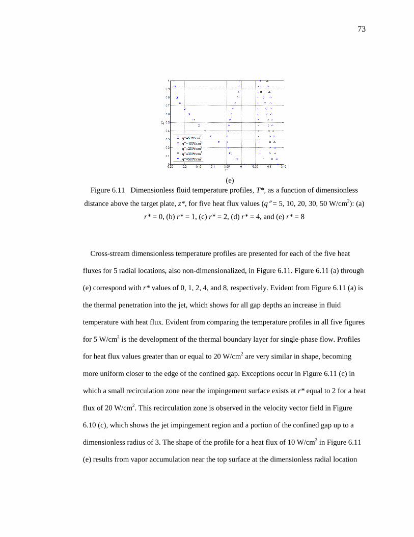
73

(e)

Figure 6.11 Dimensionless fluid temperature profiles, T*, as a function of dimensionless

distance above the target plate, z*, for five heat flux values (q″ = 5, 10, 20, 30, 50 W/cm2): (a)

r* = 0, (b) r* = 1, (c) r* = 2, (d) r* = 4, and (e) r* = 8

Cross-stream dimensionless temperature profiles are presented for each of the five heat

fluxes for 5 radial locations, also non-dimensionalized, in Figure 6.11. Figure 6.11 (a) through

(e) correspond with r* values of 0, 1, 2, 4, and 8, respectively. Evident from Figure 6.11 (a) is

the thermal penetration into the jet, which shows for all gap depths an increase in fluid

temperature with heat flux. Evident from comparing the temperature profiles in all five figures

for 5 W/cm2 is the development of the thermal boundary layer for single-phase flow. Profiles

for heat flux values greater than or equal to 20 W/cm2 are very similar in shape, becoming

more uniform closer to the edge of the confined gap. Exceptions occur in Figure 6.11 (c) in

which a small recirculation zone near the impingement surface exists at r* equal to 2 for a heat

flux of 20 W/cm2. This recirculation zone is observed in the velocity vector field in Figure

6.10 (c), which shows the jet impingement region and a portion of the confined gap up to a

dimensionless radius of 3. The shape of the profile for a heat flux of 10 W/cm2 in Figure 6.11

(e) results from vapor accumulation near the top surface at the dimensionless radial location

74

equals to 8. Vapor contours at this location and these conditions are not shown in the present

document.

(a) (b) Figure 6.12 Dimensionless radial velocity profiles, ky∗, as a function of dimensionless

distance above the target plate, z*, for five heat flux values (q″ = 5, 10, 20, 30, 50 W/cm2): (a)

r* = 1 and (b) r* = 2

Non-dimensional radial velocity profiles for all five heat fluxes are provided in Figure 6.12

at two dimensionless radial locations: (a) r* = 1 and (b) r* = 2. Near the jet edge, observed in

Figure 6.12 (a), the fluid velocities are not considerably influenced by heat flux because

significant vapor quantities are not yet generated. At a dimensionless radial distance equal to

2, small recirculation regions are observed near the confining wall and the target surface for

the single-phase case of 5 W/cm2. With an increase in heat flux to 10 W/cm2, the top

recirculation zone increases in strength (i.e. negative velocity) whereas the recirculation zone

near the target surface disappears. Increasing the heat flux to 20 W/cm2 yields a larger, in

terms of depth z*, recirculation region near the confining surface.

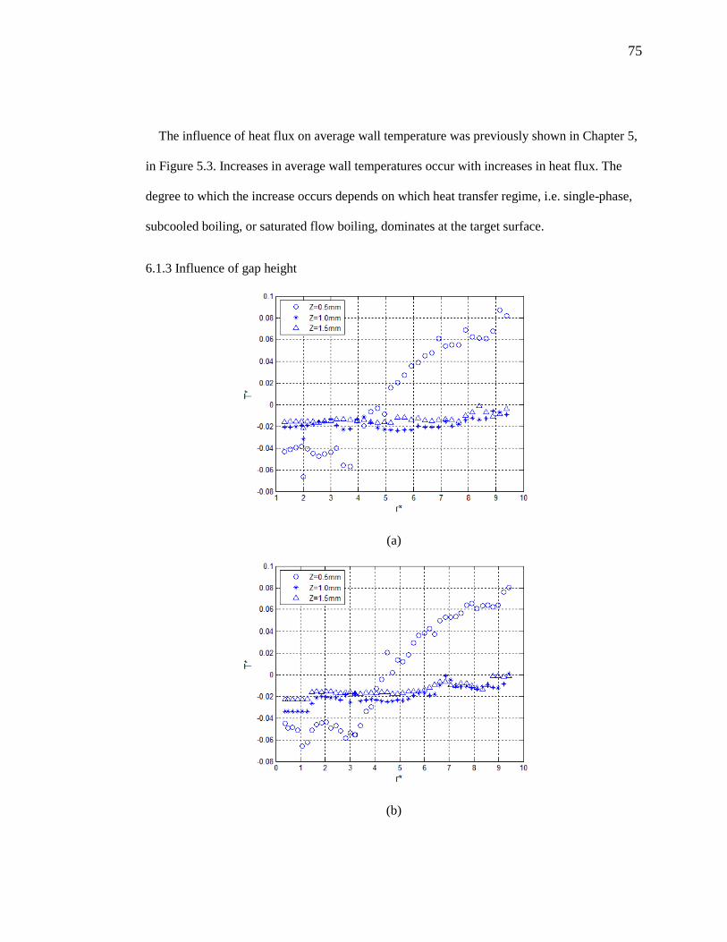
75

The influence of heat flux on average wall temperature was previously shown in Chapter 5,

in Figure 5.3. Increases in average wall temperatures occur with increases in heat flux. The

degree to which the increase occurs depends on which heat transfer regime, i.e. single-phase,

subcooled boiling, or saturated flow boiling, dominates at the target surface.

6.1.3 Influence of gap height

(a)

(b)

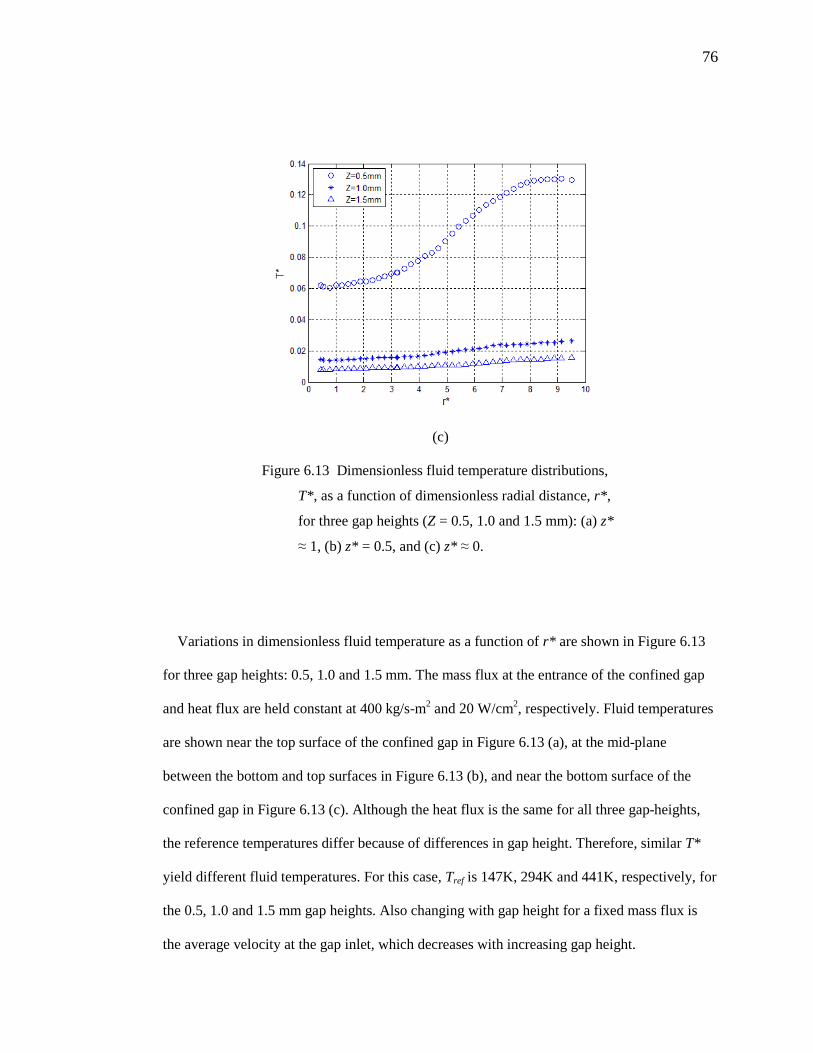
76

(c)

Figure 6.13 Dimensionless fluid temperature distributions,

T*, as a function of dimensionless radial distance, r* ,

for three gap heights (Z = 0.5, 1.0 and 1.5 mm): (a) z*

≈ 1, (b) z* = 0.5, and (c) z* ≈ 0.

Variations in dimensionless fluid temperature as a function of r* are shown in Figure 6.13

for three gap heights: 0.5, 1.0 and 1.5 mm. The mass flux at the entrance of the confined gap

and heat flux are held constant at 400 kg/s-m2 and 20 W/cm2, respectively. Fluid temperatures

are shown near the top surface of the confined gap in Figure 6.13 (a), at the mid-plane

between the bottom and top surfaces in Figure 6.13 (b), and near the bottom surface of the

confined gap in Figure 6.13 (c). Although the heat flux is the same for all three gap-heights,

the reference temperatures differ because of differences in gap height. Therefore, similar T*

yield different fluid temperatures. For this case, Tref is 147K, 294K and 441K, respectively, for

the 0.5, 1.0 and 1.5 mm gap heights. Also changing with gap height for a fixed mass flux is

the average velocity at the gap inlet, which decreases with increasing gap height.

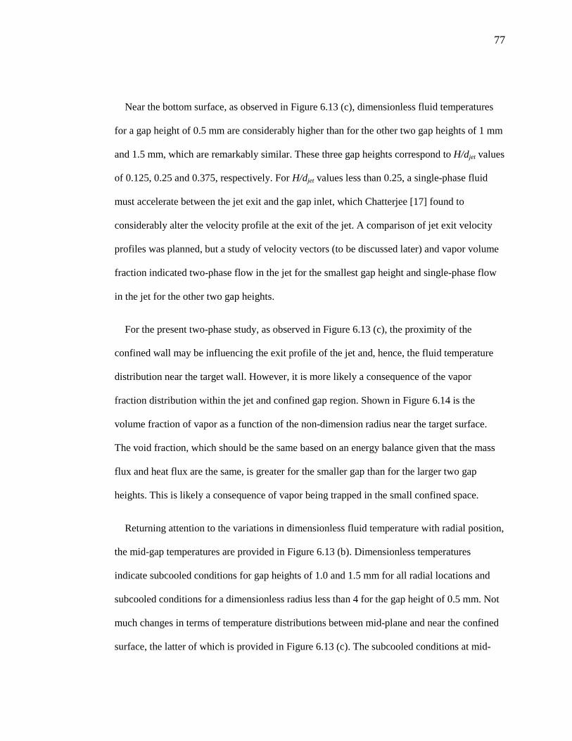
77

Near the bottom surface, as observed in Figure 6.13 (c), dimensionless fluid temperatures

for a gap height of 0.5 mm are considerably higher than for the other two gap heights of 1 mm

and 1.5 mm, which are remarkably similar. These three gap heights correspond to H/djet values

of 0.125, 0.25 and 0.375, respectively. For H/djet values less than 0.25, a single-phase fluid

must accelerate between the jet exit and the gap inlet, which Chatterjee [17] found to

considerably alter the velocity profile at the exit of the jet. A comparison of jet exit velocity

profiles was planned, but a study of velocity vectors (to be discussed later) and vapor volume

fraction indicated two-phase flow in the jet for the smallest gap height and single-phase flow

in the jet for the other two gap heights.

For the present two-phase study, as observed in Figure 6.13 (c), the proximity of the

confined wall may be influencing the exit profile of the jet and, hence, the fluid temperature

distribution near the target wall. However, it is more likely a consequence of the vapor

fraction distribution within the jet and confined gap region. Shown in Figure 6.14 is the

volume fraction of vapor as a function of the non-dimension radius near the target surface.

The void fraction, which should be the same based on an energy balance given that the mass

flux and heat flux are the same, is greater for the smaller gap than for the larger two gap

heights. This is likely a consequence of vapor being trapped in the small confined space.

Returning attention to the variations in dimensionless fluid temperature with radial position,

the mid-gap temperatures are provided in Figure 6.13 (b). Dimensionless temperatures

indicate subcooled conditions for gap heights of 1.0 and 1.5 mm for all radial locations and

subcooled conditions for a dimensionless radius less than 4 for the gap height of 0.5 mm. Not

much changes in terms of temperature distributions between mid-plane and near the confined

surface, the latter of which is provided in Figure 6.13 (c). The subcooled conditions at mid-

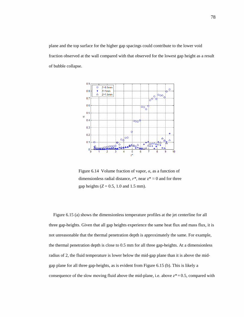
78

plane and the top surface for the higher gap spacings could contribute to the lower void

fraction observed at the wall compared with that observed for the lowest gap height as a result

of bubble collapse.

Figure 6.14 Volume fraction of vapor, α, as a function of

dimensionless radial distance, r* , near z* ≈ 0 and for three

gap heights (Z = 0.5, 1.0 and 1.5 mm).

Figure 6.15 (a) shows the dimensionless temperature profiles at the jet centerline for all

three gap-heights. Given that all gap heights experience the same heat flux and mass flux, it is

not unreasonable that the thermal penetration depth is approximately the same. For example,

the thermal penetration depth is close to 0.5 mm for all three gap-heights. At a dimensionless

radius of 2, the fluid temperature is lower below the mid-gap plane than it is above the mid-

gap plane for all three gap-heights, as is evident from Figure 6.15 (b). This is likely a

consequence of the slow moving fluid above the mid-plane, i.e. above z* = 0.5, compared with

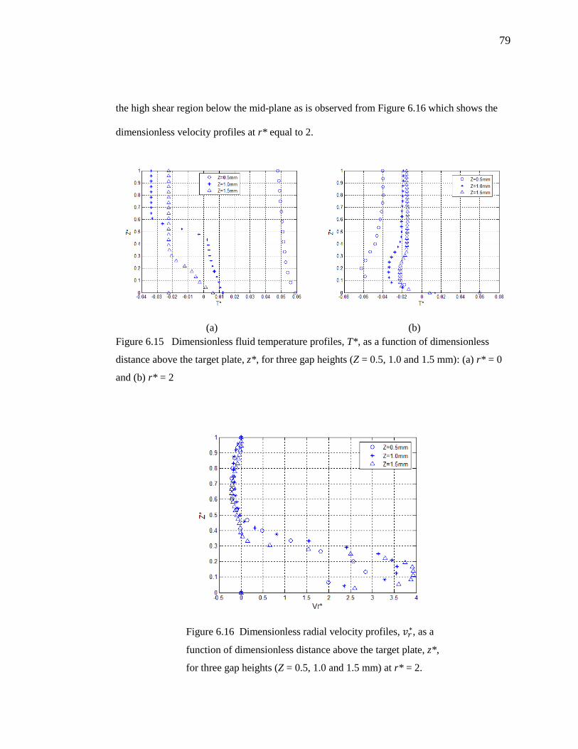
79

the high shear region below the mid-plane as is observed from Figure 6.16 which shows the

dimensionless velocity profiles at r* equal to 2.

(a) (b) Figure 6.15 Dimensionless fluid temperature profiles, T*, as a function of dimensionless

distance above the target plate, z*, for three gap heights (Z = 0.5, 1.0 and 1.5 mm): (a) r* = 0

and (b) r* = 2

Figure 6.16 Dimensionless radial velocity profiles, ky∗, as a

function of dimensionless distance above the target plate, z*,

for three gap heights (Z = 0.5, 1.0 and 1.5 mm) at r* = 2.

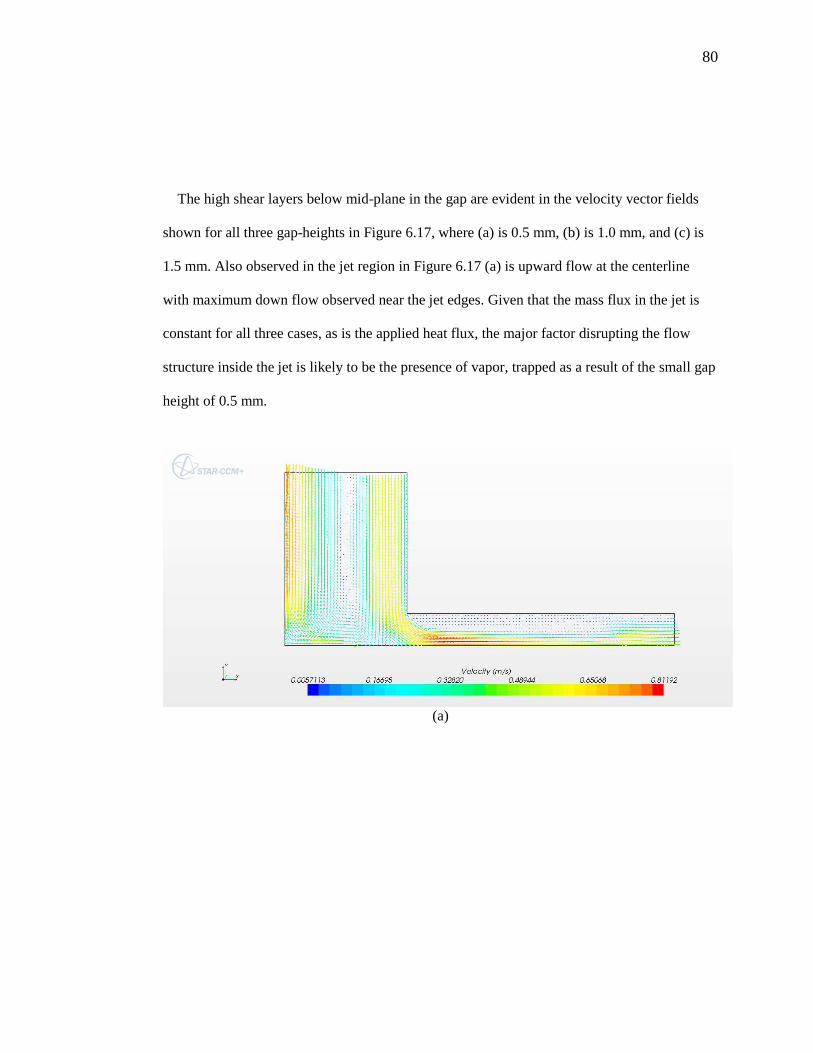
80

The high shear layers below mid-plane in the gap are evident in the velocity vector fields

shown for all three gap-heights in Figure 6.17, where (a) is 0.5 mm, (b) is 1.0 mm, and (c) is

1.5 mm. Also observed in the jet region in Figure 6.17 (a) is upward flow at the centerline

with maximum down flow observed near the jet edges. Given that the mass flux in the jet is

constant for all three cases, as is the applied heat flux, the major factor disrupting the flow

structure inside the jet is likely to be the presence of vapor, trapped as a result of the small gap

height of 0.5 mm.

(a)

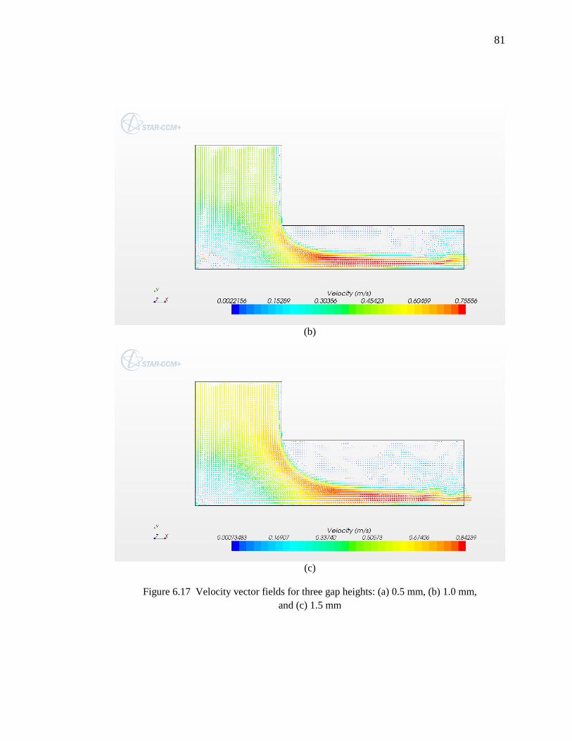
81

(b)

(c)

Figure 6.17 Velocity vector fields for three gap heights: (a) 0.5 mm, (b) 1.0 mm, and (c) 1.5 mm

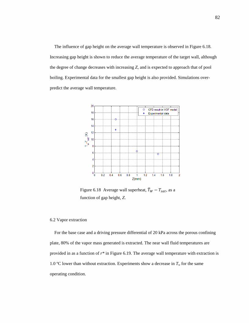
82

The influence of gap height on the average wall temperature is observed in Figure 6.18.

Increasing gap height is shown to reduce the average temperature of the target wall, although

the degree of change decreases with increasing Z, and is expected to approach that of pool

boiling. Experimental data for the smallest gap height is also provided. Simulations over-

predict the average wall temperature.

Figure 6.18 Average wall superheat, J − b2, as a

function of gap height, Z.

6.2 Vapor extraction

For the base case and a driving pressure differential of 20 kPa across the porous confining

plate, 80% of the vapor mass generated is extracted. The near wall fluid temperatures are

provided in as a function of r* in Figure 6.19. The average wall temperature with extraction is

1.0 ºC lower than without extraction. Experiments show a decrease in Tw for the same

operating condition.

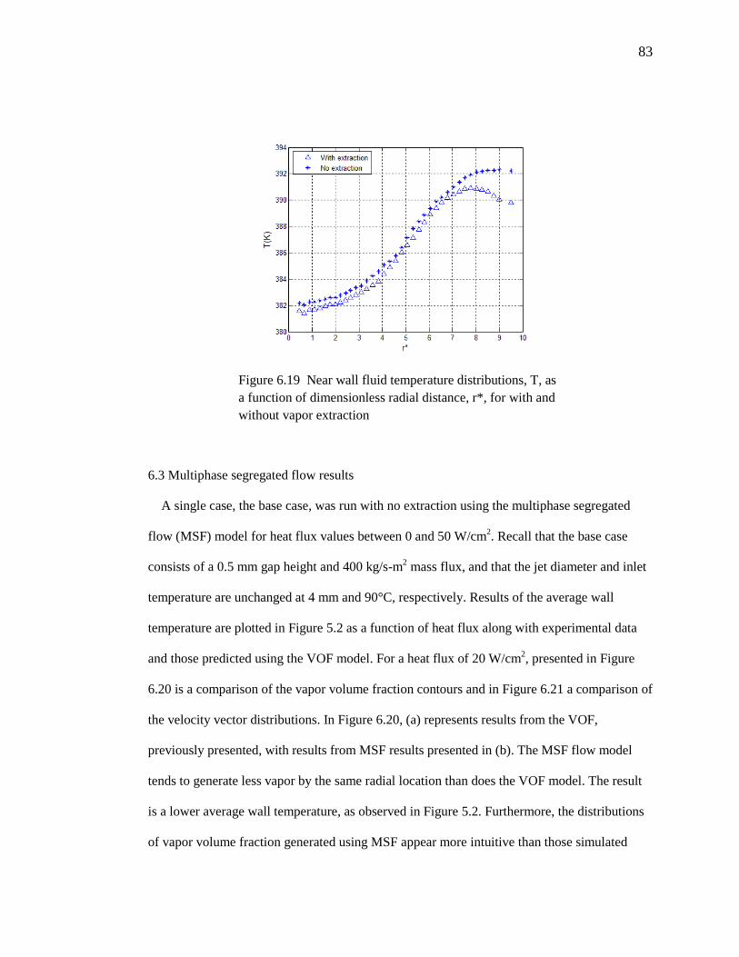
83

Figure 6.19 Near wall fluid temperature distributions, T, as a function of dimensionless radial distance, r*, for with and without vapor extraction

6.3 Multiphase segregated flow results

A single case, the base case, was run with no extraction using the multiphase segregated

flow (MSF) model for heat flux values between 0 and 50 W/cm2. Recall that the base case

consists of a 0.5 mm gap height and 400 kg/s-m2 mass flux, and that the jet diameter and inlet

temperature are unchanged at 4 mm and 90°C, respectively. Results of the average wall

temperature are plotted in Figure 5.2 as a function of heat flux along with experimental data

and those predicted using the VOF model. For a heat flux of 20 W/cm2, presented in Figure

6.20 is a comparison of the vapor volume fraction contours and in Figure 6.21 a comparison of

the velocity vector distributions. In Figure 6.20, (a) represents results from the VOF,

previously presented, with results from MSF results presented in (b). The MSF flow model

tends to generate less vapor by the same radial location than does the VOF model. The result

is a lower average wall temperature, as observed in Figure 5.2. Furthermore, the distributions

of vapor volume fraction generated using MSF appear more intuitive than those simulated

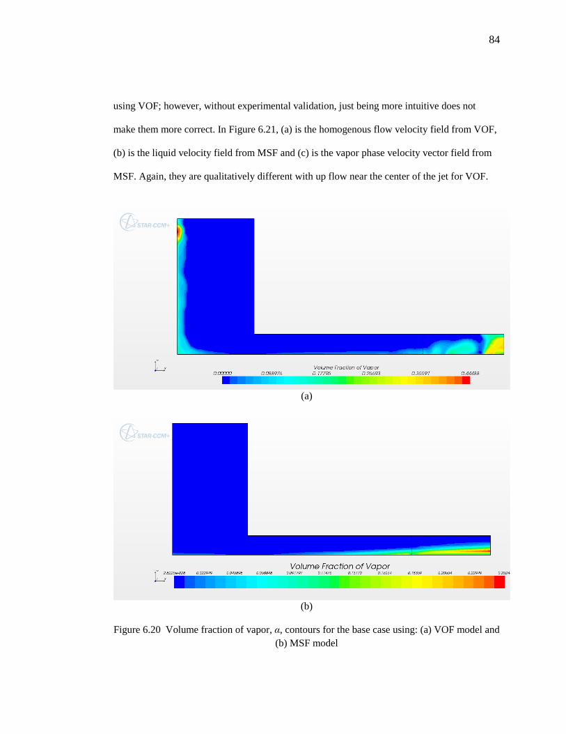
84

using VOF; however, without experimental validation, just being more intuitive does not

make them more correct. In Figure 6.21, (a) is the homogenous flow velocity field from VOF,

(b) is the liquid velocity field from MSF and (c) is the vapor phase velocity vector field from

MSF. Again, they are qualitatively different with up flow near the center of the jet for VOF.

(a)

(b)

Figure 6.20 Volume fraction of vapor, α, contours for the base case using: (a) VOF model and (b) MSF model

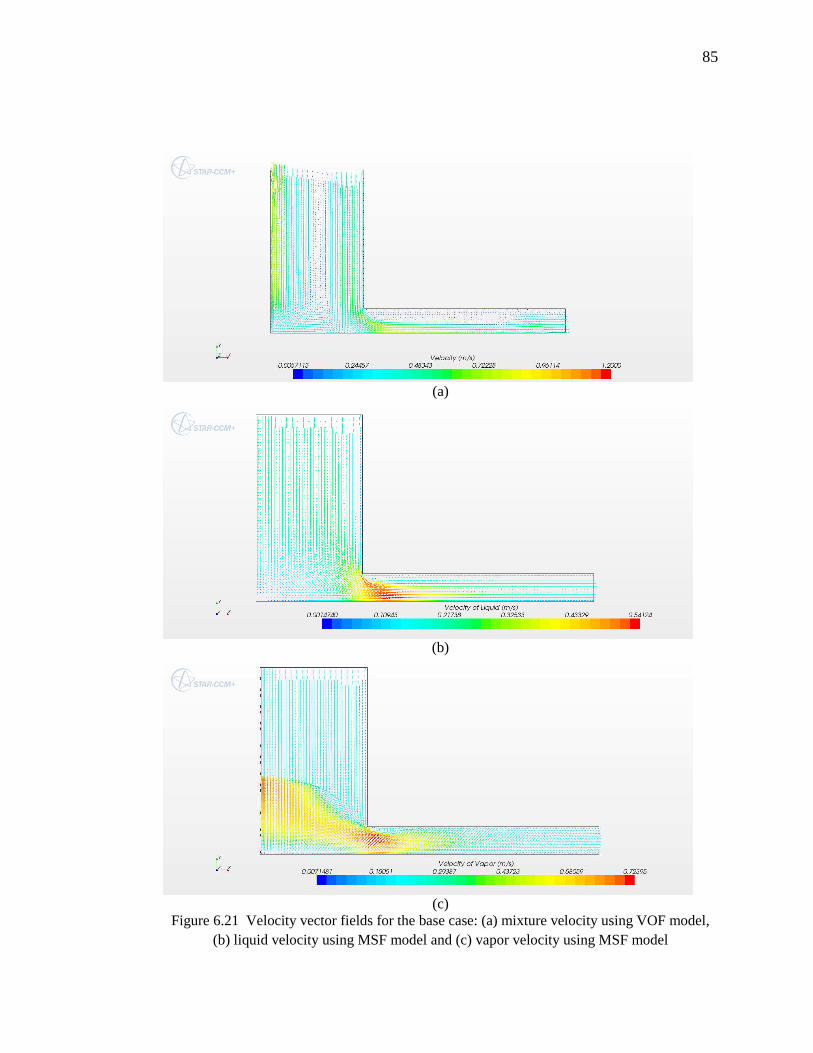
85

(a)

(b)

(c)

Figure 6.21 Velocity vector fields for the base case: (a) mixture velocity using VOF model, (b) liquid velocity using MSF model and (c) vapor velocity using MSF model

86

6.4 Discussion

The ultimate goal is to simulate vapor extraction. On the positive side, recall that a pressure

differential can be applied across a porous wall in the VOF model. A static contact angle,

rather a user-defined algorithm, was assigned to the top and bottom walls to prevent passage

of the liquid, also known as breakthrough, through the porous wall. The VOF method requires

the exit volume fraction of vapor be specified, rather than being extrapolated from the interior.

The value to be specified was determined using a global energy balance and a void fraction

(volume fraction of vapor) correlation. Simulated volume fractions near the exit could be

different enough from those specified at the exit to cause unreasonable flow phenomena. The

volume fraction at the exit was then changed to a value midway between theory and simulated

results, and the solution was then rerun and iterated. Furthermore, the fraction of energy

supplied that contributed to vapor generation had to be specified. As this fraction increases

beyond 0.1, the vapor generation approaches the theoretical values whereas the wall superheat

further exceeded experiments.

In the case of the MSF model, the vapor fraction at the gap exit can be extrapolated rather

than imposed. Vapor generated without extraction using the MSF model is closer to

theoretical values than vapor generated using the VOF model. However, because the amount

of vapor that is passed through the porous wall is specified and not solved in the MSF model,

it was deemed less desirable than the VOF model.

Unfortunately, as currently programmed, neither model is ideally suited for the desired

purpose, which is modeling two-phase confined flow boiling with vapor extraction. Ideally,

the porous wall option from the VOF model could be coupled with the MSF model.

Furthermore, it would be desirable to perform flow visualization or at least make more

87

accurate, spatially resolved temperature distributions along the target plate to properly validate

the model results.

88

Chapter 7 – Conclusions and Recommendations

A computational study was conducted for a single, two-phase, axisymmetric, confined

impinging jet using the volume of fluid method (VOF). The exit of the jet was submerged and

water was the fluid used. Flow was laminar throughout. Effects of mass flux (200, 400, 800

kg/s-m2), heat flux (5, 10, 20, 30, 50 W/cm2), and gap height (0.5, 1.0, 1.5 mm) were

considered for a single diameter of 4 mm and a single inlet jet temperature of 90°C. The target

surface was an aluminum block 38 mm in diameter and 16 mm thick, with heat applied to the

bottom. Flow through the entire length of the jet was simulated with an exit of the confined

gap set to an anticipated condition expected in the exit plenum.

Simulation results for a base case were compared to experimental data. Simulations over-

predict the average temperature of the impinging surface and under-predict vapor generation.

Matching both was not achieved; therefore, results have not been validated. For conditions in

which boiling occurred in the smallest gap height of 0.5, corresponding to a height-to-jet

diameter ratio of 0.125, vapor flowed back into the jet inlet. Although this flow phenomenon

cannot be verified using this inference, significant pressure oscillations inside the jet near the

exit were observed experimentally for similar test conditions decreasing with increasing gap

height.

Recirculation zones near the gap inlet and distortions to the velocity profile at the jet exit

were observed as the gap height was varied. However, trends observed here are not consistent

with data available in the literature, as these correlations and observations are primarily

available for single-phase impinging jets.

89

Preliminary attempts of vapor extraction using the VOF method required application of a

pressure differential across, and setting viscous and inertia resistances through, a porous

confinement surface. Better estimates of the resistances are needed to better reflect

experimental results.

Finally, flow and heat transfer for the base case conditions were simulated using a different

Eulerian multiphase flow model known as the multiphase segregated flow (MSF) model.

Results were more intuitively correct, but yielded impingement wall temperatures and vapor

generation values slightly closer to experimental results than those modeled using VOF.

Unfortunately, modeling of extraction using Start CCM+ version 7.04 and the MSF model

would not be based on the Darcy flow expected.

90

Bibliography

1. C.Y. Li and S.V. Garimella, 2001. “Prandtl number effects and generalized correlations for confined and submerged jet impingement”. Purdue Libraries: Research Publications.

2. Janice A. Fitzgerald and Suresh V. Garimella, 1998. “A study of the flow field of a confined and submerged impinging jet”. International Journal of Heat and Mass Transfer, Vol. 41, Nos. 8-9, pp.1025-1034.

3. S.V. Garimella and R.A. Rice, 1995. “Confined and submerged liquid jet impingement heat transfer”. ASME Journal of Heat Transfer, Vol.117, pp.871-877.

4. Jung-Yang San, Chin-Hao Huang and Ming-Hong Shu, 1997. “Impingement cooling of a confined circular air jet”. International Journal of Heat and Mass Transfer, Vol.40, NO.6, pp.1355-1364.

5. M.F. Koseoglu and S. Baskaya, 2008. “The effect of flow field and turbulence on heat transfer characteristics of confined circular and elliptic impinging jets”. International Journal of Thermal Sciences, Vol. 47, pp. 1332-1346.

6. D.W. Colucci and R. Viskanta, 1996. “Effect of nozzle geometry on local convective heat transfer to a confined impinging air jet”. Experimental Thermal and Fluid Science, Vol. 13, pp.71-80.

7. C.T. Chang, G. Kojasoy, F. Landis, S. Downing, 1995. “Confined single-and multiple –jet impingement heat transfer--I. Turbulent submerged liquid jets”. International Journal of Heat and Mass Transfer, Vol.38, NO.5, pp.833-842.

8. N. Zuckerman and N. Lior, 2006. “Jet impingement heat transfer: physics, correlations, and numerical modeling”. Advances in Heat Transfer, Vol. 39, pp. 565-631.

9. M. Behnia, S. Parneix, Y. Shabany, P.A. Durbin, 1999. “Numerical study of turbulent heat transfer in confined and unconfined impinging jets”. International Journal of Heat and Fluid Flow, Vol. 20, pp. 1-9.

10. E. Baydar and Y. Ozmen, 2005. “An experimental and numerical investigation on a confined impinging air jet at high Reynolds numbers”. Applied Thermal Engineering, Vol. 25, pp. 409-421.

11. E. Baydar and Y. Ozmen, 2006. “An experimental investigation on flow structures of confined and unconfined impinging air jets”. Heat and Mass Transfer, Vol. 42, NO. 4, pp. 338-346.

12. Li Chang-geng and Zhou Jie-min, 2007. “Experimental and numerical simulation

91

study of heat transfer due to confined impinging circular jet”. Chemical Engineering Technology, Vol. 30, NO. 10, pp. 1355-1361.

13. Y.Q. Zu, Y.Y. Yan, J. Maltson, 2009. “Numerical study on stagnation point heat transfer by jet impingement in a confined narrow gap”. Journal of Heat Transfer, Vol. 131, pp. 0945041-0945044.

14. Deborah V. Pence, Paul A. Boeschoten, James A. Liburdy, 2003. “Simulation of compressible micro-scale jet impingement heat transfer”. Journal of Heat Transfer, Vol.125, pp.447-453.

15. Koichi Ichimiya, Shoichi Takema, Shunichi Morimoto, Tomoaki, Kunugi and Norio Akino, 2001. “Movement of impingement heat transfer by a single circular jet with a confined wall”. International Journal of Heat and Mass Transfer, Vol.44, pp.3095-3102.

16. Ajay Chatterjee and L.J. Deviprasath, 2001. “Heat transfer in confined laminar axisymmetric impinging jets at small nozzle-plate distances: the role of upstream vorticity diffusion”. Numerical Heat Transfer, Par A. Vol. 39, pp. 777-800.

17. Ajay Chatterjee, 2000. “Newtonian radial entrance flow”. AIChE Journal, Vol. 46, NO. 3, pp. 462-475.

18. Ajay Chatterjee, 2008. “Multiple vortex formation in steady laminar axisymmetric impinging flow”. Computers and Fluids, Vol. 37, pp. 1061-1076.

19. K. Nakabayashi, T. Ichikawa, Y. Morinishi, 2002. “Size of annular separation bubble around the inlet corner and viscous flow structure between two parallel disks”. Experiments in Fluids, Vol. 32, pp. 425-433.

20. Nirmalendu Biswas, Nirmal Kumar Manna, Achintya Mukhopadhyay, Swarnendu Sen, 2012. “Numerical simulation of laminar confined radial flow between parallel circular discs”. Journal of Fluids Engineering, Vol. 134, pp. 0112051-0112058.

21. C.F. Ma and A.E. Bergles, 1986. “Jet impingement nucleate boiling”. International Journal of Heat and Mass Transfer, Vol. 29, NO. 8, pp. 1095-1101.

22. D.H. Wolf, F.P. Incropera, R. Viskanta, 1996. “Local jet impingement boiling heat transfer”. International Journal of Heat and Mass Transfer, Vol. 39, NO.7, pp.1395-1460.

23. Chang Hwan Shin, Kyung Min Kim, Sung Hwan Lim, Hyung Hee Cho, 2009. “Influences of nozzle-plate spacing on boiling heat transfer of confined planar dielectric liquid impinging jet”. International Journal of Heat and Mass Transfer, Vol. 52, pp. 5293-5301.

92

24. C.T. Chang, G. Kojasoy, F. Landias, S. Downing, 1995. “Confined single- and multiple-jet impingement heat transfer--II. Turbulent two phase flow”. International Journal of Heat and Mass Transfer, Vol.38, NO.5, pp.843-851.

25. Van P. Carey, 1992. “Liquid-Vapor Phase-Change Phenomena”. Taylor and Francis, Bristol, PA.

26. D.H. Wolf, F.P. Incropera, R. Viskanta, 1993. “Jet impingement boiling”. Advances in Heat Transfer, Vol. 23, pp.1-132.

27. A.M.T. Omar, M.S. Hamad, M. Shoukri, 2009. “Modeling of nucleate boiling heat transfer under an impinging free jet”. International Journal of Heat and Mass Transfer, Vol. 52, pp. 5557-5566.

28. Sreekant Narumanchi, Andrey Troshko, Desikan Bharathan, Vahab Hassani, 2008. “Numerical simulation of nucleate boiling in impingement jets: applications in power electronics cooling”. International Journal of Heat and Mass Transfer, Vol.51, pp.1-12.

29. S. Abishek, R. Narayanaswamy, V. Narayanan, 2012. “Effect of heater size on confined subcooled jet impingement boiling”. Proceedings of the ASME 2012 Summer Heat Transfer Conference. HT2012-58205.

30. Dennis Desheng Meng, Joonwon Kim, Chang-Jin Kim, 2006. “A degassing plate with hydrophobic bubble capture and distributed venting for microfluidic devices”. Journal of Micromechanics and Microengineering, Vol. 16, pp. 419-424.

31. Dennis Desheng Meng, Thomas Cubaud, Chih-Ming Ho, and Chang-Jin Kim, 2007. “A methanol-tolerant gas-venting microchannel for a microdirect methanol fuel cell”. Journal of Microelectromechanical systems, Vol. 16, No. 6, pp. 1403-1410.

32. Yousef Alyousef and S.C. Yao, 2006. “Development of a silicon-based wettability controlled membrane for microscale direct methanol fuel cells”. Microfluid Nanofluid, Vol. 2, pp. 337-344.

33. Jia Xu, Regis Vaillant, Daniel Attinger, 2010. “Use of a porous membrane for gas bubble removal in microfluidic channels: physical mechanisms and design criteria”. Microfluidics and Nanofluidics, Vol. 9, Issue 4-5, pp. 765-772.

34. Brentan R. Alexander and Evelyn N. Wang, 2009. “Design of a microbreather for two-phase microchannel heat sinks”. Nanoscale and Microscale Thermophysical Engineering, Vol. 13, pp. 151-164.

35. Milne P. David, Julie E. Steinbrenner, Josef Miler, Kenneth E. Goodson, 2011. “Adiabatic and diabatic two-phase venting flow in a microchannel”. International Journal of Multiphase Flow, Vol.37, pp.1135-1146.

93

36. Milne P. David, Josef Miler, Julie E. Steinbrenner, Yizhang Yang, Maxat Touzelbaev, Kenneth E. Goodson, 2011. “Hydraulic and thermal characteristics of a vapor venting two-phase microchannel heat exchanger”. International Journal of Heat and Mass Transfer, Vol.54, pp.5504-5516.

37. Amy M. Marconnet, Milne P. David, Anita Gogacs, Roger D. Flynn, Kenneth E. Goodson, 2008. “Temperature-dependent permeability of microporous membranes for vapor venting heat exchangers”. Proceedings of 2008 ASME international mechanical engineering congress and exposition, IMECE 2008.

38. Chen Fang, Milnes David, Anita Rogacs, Kenneth Goodson, 2010. “Volume of fluid simulation of boiling two-phase flow in a vapor-venting microchannel”. Frontiers in Heat and Mass Transfer.

39. M. Sabo, 2012. “Performance and Flow Stability Characteristics in Two-Phase Confined Impinging Jets”. M. S. thesis. Oregon State University.

94

APPENDICES

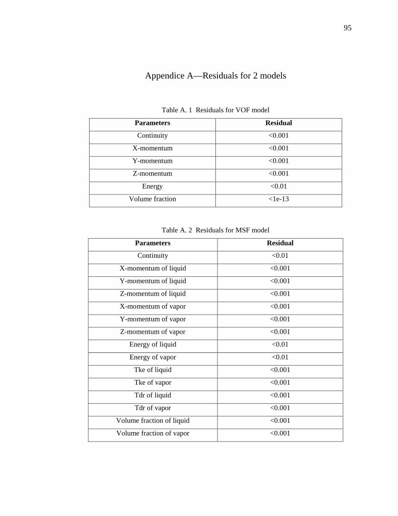
95

Appendice A—Residuals for 2 models

Table A. 1 Residuals for VOF model

Parameters Residual

Continuity <0.001

X-momentum <0.001

Y-momentum <0.001

Z-momentum <0.001

Energy <0.01

Volume fraction <1e-13

Table A. 2 Residuals for MSF model

Parameters Residual

Continuity <0.01

X-momentum of liquid <0.001

Y-momentum of liquid <0.001

Z-momentum of liquid <0.001

X-momentum of vapor <0.001

Y-momentum of vapor <0.001

Z-momentum of vapor <0.001

Energy of liquid <0.01

Energy of vapor <0.01

Tke of liquid <0.001

Tke of vapor <0.001

Tdr of liquid <0.001

Tdr of vapor <0.001

Volume fraction of liquid <0.001

Volume fraction of vapor <0.001

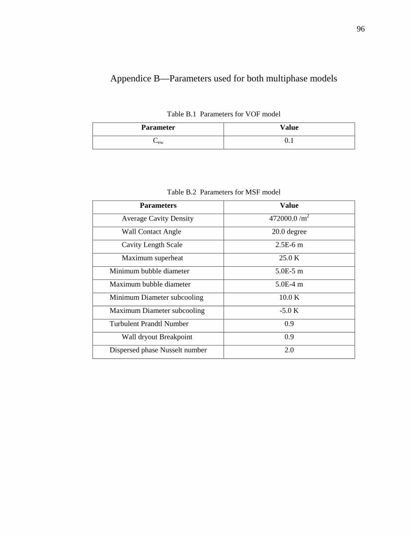
96

Appendice B—Parameters used for both multiphase models

Table B.1 Parameters for VOF model

Parameter Value

Cew 0.1

Table B.2 Parameters for MSF model

Parameters Value

Average Cavity Density 472000.0 /m2

Wall Contact Angle 20.0 degree

Cavity Length Scale 2.5E-6 m

Maximum superheat 25.0 K

Minimum bubble diameter 5.0E-5 m

Maximum bubble diameter 5.0E-4 m

Minimum Diameter subcooling 10.0 K

Maximum Diameter subcooling -5.0 K

Turbulent Prandtl Number 0.9

Wall dryout Breakpoint 0.9

Dispersed phase Nusselt number 2.0