health and development - theigc.org
TRANSCRIPT

Labor, Health and Development
Nidhiya Menon
IGC Summer School,
New Delhi, July 2015

Outline of lecture
1. Why labor and health are important topics within development economics
2. Determinants of labor and health
3. Impacts on labor and health
– Water pollution
– Impacts of regulating pollution in India

Health and productivity as means to higher income
Income
Health Labor productivity

Mortality versus GDP

Large role of government
• Government plays a large role in labor and health sectors
• A great deal of policy-making in these arenas

Why is government so involved?
• Basic rights that society wants to guarantee to its citizens
• Externalities – Technological progress (e.g., productive people
generate ideas) – Infectious diseases – Environment/pollution impacts
• Break intergenerational transmission of poverty – Want to lift people out of poverty permanently – Difficult to raise earnings capacity of an adult after
health status is largely determined

Labour, Nutrition and Productivity
Ray – Chapter 13

1. Types of hired labor
(a) Laborers that are hired on a casual basis, perhaps on some daily arrangement
(b) Laborers that are under some long term contract with their employer.
Makes sense to think of two different types of labor based or the scope for “punishing”. The scope for “punishing” the casual employee is much lower.
With a long term employee, future employment may be denied or the terms of employment may be modified.
Types of Labor

Types of Labor (cont’d)
This argument leads to a puzzle since standard supply and demand models of the labor market tells us that the labor market will “clear” at a wage that mirrors accurately the opportunity cost of the workers time If denied employment, the worker can find employment elsewhere at the same wage, or even if the worker is unemployed, the utility of the additional leisure just compensates for the loss in wages Thus, the employer has no additional power over a long-term employee The standard model may be inappropriate for thinking about long-term relationships


• Demand curve for labor – depends on the nominal wage (measured by w). If w decreases, the demand for labor increases (or at least, does not decrease), so demand is downward sloping
• Supply curve – a higher wage rate elicits a greater supply of labor from each worker, as well as encourages a larger number of workers to enter the labor market. Supply curve is upward sloping

• The standard story assumes that all work is perfectly monitor-able
• Rural labor markets are characterized by substantial uncertainty and/or seasonality.
We can incorporate this is the standard story. Suppose rainfall levels are uncertain and this will affect the size of the harvest. So the labor demand curve itself is uncertain, it fluctuates between the highs and lows described by the dotted line.
Thus the equilibrium wage fluctuations lie between a band of WH and WL

Wage Rate vs. Labor

• This does not illustrate the possible ways in which employees and employers can cope with this uncertainty “before the fact” – by writing contracts or making informal agreements that insure one
party or the other from the effects of rainfall variation.
• Similarly workers may wish to smooth out seasonal fluctuations in their wage income – employers who are willing to provide said income smoothing may be
preferred by employees

Poverty, Nutrition, and Labor Markets
• Think of a relationship between nutrition and work capacity which we call the capacity curve
• Horizontal axis is labelled “income” since our implicit assumption is that all income is consumed
• Vertical axis – think of it as a measure of the total number of tasks an individual can perform during a given period, eg. number of bushels of wheat that he can harvest during a day

Capacity Curve

Piece Rates
• Piece rates
– Income determines work capacity, but work capacity determines income as well.
• Piece rate appears as a relationship between the number of tasks performed and total income


• Suppose that laborer T tries to obtain the highest possible level of income, given the restraints imposed by his capacity curve. If the going rate is V1, T chooses point A
• As rate decreases to V2, he moves to B which involves less total work and lower income

Work Capacity vs. Income

• V3 is a piece rate that is just tangent to the capacity curve, and so T chooses point C. If the rate drops a little more, then the amount of work T supplies drops dramatically from C to D (intersection of the lowest piece rate and the capacity curve)
• This jump occurs because of the shape of the capacity curve with low levels of nutrition permitting only very low levels of work, and moderate to high levels creating a rapid increase in work capacity
• Use all this information to generate a labor supply curve – Multiply T’s labor supply (at each piece rate) by the number of
workers like him in the economy

Labor Supply Curve

• The gap in the labor supply at V3 captures T’s jump in labor supply. The R.H.S. panel depicts the situation for aggregate supply
• Now introduce a standard demand curve and analyze 2 situations:

Labor Supply Curve
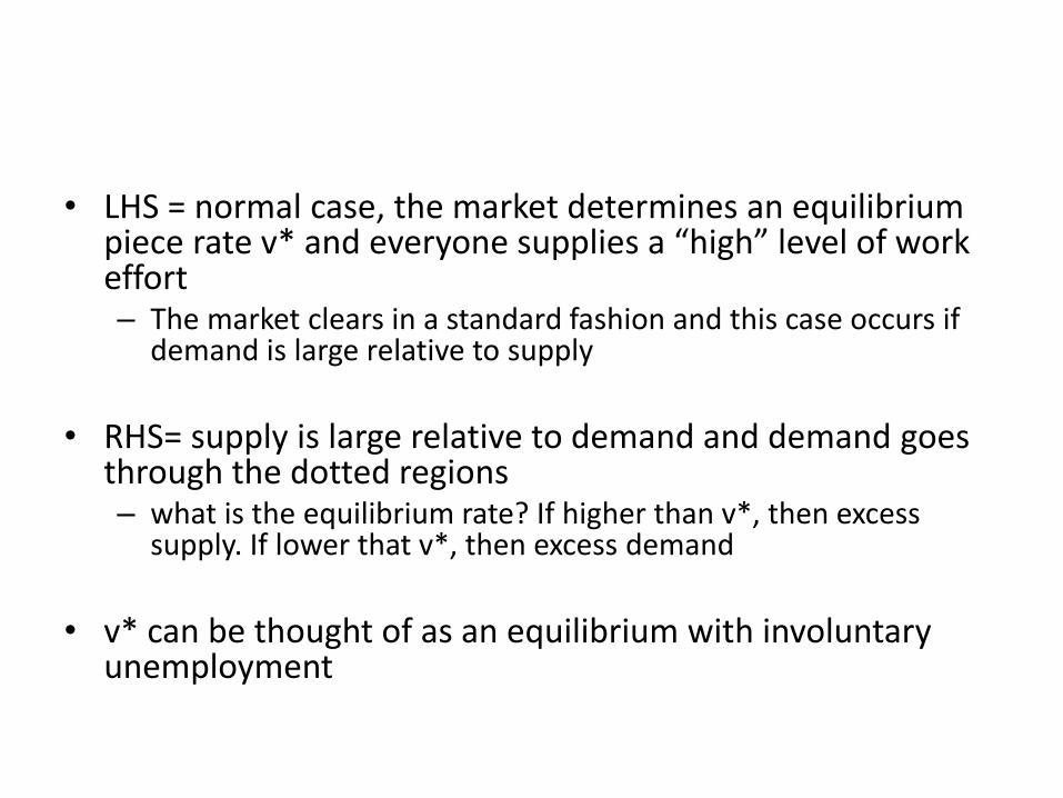
• LHS = normal case, the market determines an equilibrium piece rate v* and everyone supplies a “high” level of work effort – The market clears in a standard fashion and this case occurs if
demand is large relative to supply
• RHS= supply is large relative to demand and demand goes
through the dotted regions – what is the equilibrium rate? If higher than v*, then excess
supply. If lower that v*, then excess demand
• v* can be thought of as an equilibrium with involuntary
unemployment

• This unemployment is involuntary in the sense that people want to work but cannot – but the piece rate cannot be bid down because no one
can “credibly” supply the same amount of labor at a lower rate
• Thus we have a vicious cycle – wages determine work capacity but low capacity to
work feeds back on itself by lowering access to labor markets

Non-labor assets and the labor market
• Realistically, people have other sources of income, so it is not completely accurate to equate total income with wages, eg: individuals may have tiny landholding that are leased out

Work Capacity vs. Wage Income

Inequalities in assets
• Think of another worker S who has access to a source of non-labor income of size R (e.g.: rent). – So work capacity now depends on rent plus wages. Since the horizontal axis
involves only wage income, we can shift the capacity curve horizontally to the left by the amount R
• Superimpose the diagram on the picture for T who has no sources of non-labor income
• Note that although T may be biologically just the same as S, his capacity curve lies to the right and below that of S who has land rents
• First, under V1, T is only able to supply a small amount of labor for the same reason as before, he is effectively excluded from the labor market

Inequalities in assets
• S can supply at V1
• Even if the piece rates are so high that both can supply labor (as in the case of v2), note that S is still earning a higher income than T
• The larger size of S’s income is not just because of his non-labor assets; he earns higher wage income also
• Thus inequalities in the asset market magnify further into labor market inequalities

Types of research questions
• We would like to know how to improve health and labor market performance
• Example 1: Unintended health consequences of good ideas – How water pollution from fertilizers affects infant
health
• Example 2: Can air and water pollution be regulated to improve health? – Are there measurable declines?
– How air and water pollution may affect infant health

Seasonal Effects of Water Quality: The Hidden
Costs of the Green Revolution to Infant and
Child Health in India
Brainerd and Menon

Motivation
• Green Revolution (1965-late 1970s)
– increased agricultural production and helped achieve food security
– exacted a toll on the country’s environment: contamination of water
– technologies: HYV seeds, “double-cropping”, irrigation, pesticides,
and nitrogenous fertilizer
– HYV seeds need more fertilizer and water than do indigenous seeds
• Synthetic nitrogen based fertilizers such as Urea and
Nitrogen-Phosphate-Potassium (NPK)
– heavily over-used
– seepage into surface and ground water through soil run-offs

Trend in consumption of NPK fertilizer in India
0
50
10
015
0
NP
K fe
rtili
zer
use
, kg
pe
r h
ect
are
1960 1970 1980 1990 2000 2010
kg per hectare of cropped area
Consumption of NPK Fertilizer,

Motivation
• Goal of study: evaluate the infant and child health implications
of exposure to fertilizer agrichemicals
– focus on fertilizers because they have relatively clear application times
– concentrations of agrichemicals in water vary seasonally
– water contamination also varies regionally (northern India plants winter
crops; southern India plants summer crops)
– focus on agrichemicals in water as it is considered a reliable measure of
human exposure

Why is this relevant?
• In rural India, women are at the forefront of farming activities
– 55-60 percent of the labor force, so directly exposed
– their children are exposed both in utero and after birth to toxins
– rates of stunting and wasting among Indian children are higher than
predicted given per capita income and infant mortality rates (Deaton
and Dreze, 2009)
• Negative externalities of motile agrichemical-contaminated
water

Why is this relevant?
• Seasonal exposure to water toxins can have inter-generational
effects
– documented link in biomedical studies between low-birth weight and
coronary heart disease which is inheritable
– transmission occurs even without any additional exposure to chemical
contaminants in water
– Behrman and Rosenzweig (2004) note importance of fetal
health/nutrition

Preview of results
• Presence of agrichemicals in water in month of conception
significantly increases infant and neo-natal mortality
– 10 percent increase leads to rise in infant mortality by about 4.6 percent
– 10 percent increase leads to rise in neo-natal mortality by about 6.2
percent
• Agrichemicals in month of conception have significant
negative impacts on height-for-age and weight-for-age z scores
as of age 5
• Negative effects are most evident for vulnerable populations
– children of uneducated poor women in rural India

Preview of results
• Some evidence that exposure beyond the first month matters
(first, second and third trimester exposure)
• Results robust to checks on instruments and omitted variables
such as rainfall, temperature, diseases, timing of conception
and parental characteristics

Cross-country comparison
• Water pollution concentrations are higher in India than in other
countries like the US or China
• Average nitrogen level in Indian water bodies significantly
exceeds levels in US and China over a comparable time period
• True even in relation to Pakistan, neighbor that shares
agricultural and socio-economic practices

Cross-country comparison of the prevalence of nitrogen
in water from 1980-1996.
0
0.5
1
1.5
2
2.5
3
US China India Pakistan
mg/l
mean nitrogen

Identification methodology
• Identify fertilizer agrichemical impacts using two sources of
variation for the main crops of rice and wheat
– exogeneity in soil endowments which makes some states more suitable
for rice and others for wheat
• bulk of wheat production – UP, Punjab, Haryana, Gujarat, Bihar,
MP
• bulk of rice production – AP, WB, Assam, Tamil Nadu, Kerala,
Orissa
– exogeneity in timing of crop cycles of each crop
• rice is mainly a kharif (monsoon) crop: sown in June-August and
reaped in autumn
• wheat is a rabi (winter) crop: sown in November-April and
harvested in spring
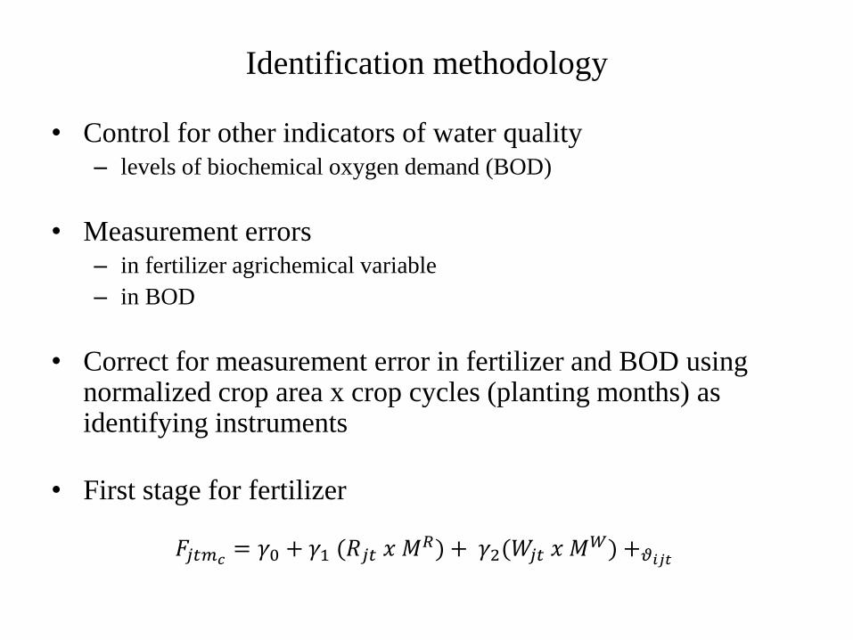
Identification methodology
• Control for other indicators of water quality
– levels of biochemical oxygen demand (BOD)
• Measurement errors
– in fertilizer agrichemical variable
– in BOD
• Correct for measurement error in fertilizer and BOD using normalized crop area x crop cycles (planting months) as identifying instruments
• First stage for fertilizer
𝐹𝑗𝑡𝑚𝑐= 𝛾0 + 𝛾1 (𝑅𝑗𝑡 𝑥 𝑀
𝑅) + 𝛾2(𝑊𝑗𝑡 𝑥 𝑀𝑊) +𝜗𝑖𝑗𝑡

Water data
• Central Pollution Control Board (CPCB) of India:
– established by the Water Act of 1974
– GEMS and MINARS programs to monitor water quality
• Location of monitoring stations:
– major rivers/tributaries, wells, lakes, creeks, ponds, canals, and tanks
throughout India
– 870 stations as of 2005

Water data
• CPCB collects statistics on:
– microbiology, nutrients, organic matter, major ions, metals, and
physical/ chemical characteristics of water
• Sources of our water data:
– UNEP/GEMS (1978 to 2005 data – subset of monitoring stations)
– CPCB electronic files (2005 only)
– Greenstone and Hanna (1986 to 2005 data – 489 stations in 424 cities)
– CPCB year books (annual data from 1978 to 2005)

Mean nitrogen concentration in water by month
from 1978-2005 for wheat
0
1
2
3
4
5
6
7
8
Jun Jul Aug Sep Oct Nov Dec Jan Feb Mar Apr May
wheat non-wheat

Mean phosphate concentration in water by month
from 1978 – 2005 for rice
0
0.1
0.2
0.3
0.4
0.5
0.6
0.7
0.8
Jun Jul Aug Sep Oct Nov Dec Jan Feb Mar Apr May
rice non-rice

Trend in biochemical oxygen demand over time
0
0.5
1
1.5
2
2.5
3
3.5
4
4.5
1992 1998 2005
mg\l
Biochemical oxygen demand

Trend in presence of fertilizer agrichemicals in water
over time
0
0.1
0.2
0.3
0.4
0.5
0.6
1992 1998 2005
mea
n o
f th
e d
um
my f
or
pre
sence
of
fert
iliz
er a
gri
chem
ical
s
Fertilizer agrichemicals

Demographic outcomes and controls
• Indian National Family Health Surveys (NFHS) from 1992,
1998, and 2005
• Questions are asked of all women between 15-49 years of age
• Repeated cross-sections with national coverage
• Information on child-specific, women-specific, and household-
specific characteristics
– month and year of conception determined by using month and year of
birth, assuming 9 month gestation cycle
• Estimation sample has child health outcomes matched with
agrichemical and BOD presence in month of conception +
other controls

Demographic outcomes and controls
• Use additional information on variables for robustness checks
from
– Economic Organization Public Policy Program database (EOPP at
LSE)
– Vital Statistics of India, various years
– Statistical Abstract of India, various years
– Directorate of Economics and Statistics, Department of Agriculture

Outcomes studied
• Considered to be most impacted in the first trimester:
– infant mortality
– neonatal mortality
– post-natal mortality
• Most impacted in other trimesters:
– height-for-age z score (stunting)
– weight-for-age z score (underweight)

Means and standard deviations of outcomes
All areas Wheat areas Rice areas
Variables Mean Std. dev. Mean Std. dev. Mean Std. dev.
Outcomes
Born alive but died before 11 months (infant mort.) 0.074 (0.034) 0.088 (0.031) 0.059 (0.034)
Born alive but died in first month (neonatal mort.) 0.048 (0.024) 0.056 (0.022) 0.039 (0.025)
Born alive but died b/w 1-11 mths. (post-natal
mort.) 0.026 (0.017) 0.032 (0.016) 0.020 (0.016)
Height-for-age z score -1.861 (1.521) -2.035 (1.546) -1.636 (1.561)
Weight-for-age z score -1.958 (1.136) -2.049 (1.149) -1.849 (1.141)

First stage regression results
• Use information on cropped area under rice in both kharif and
summer seasons
• Effects of the rice and wheat instruments may be contaminated
with time and state-level heterogeneity
• Include time dummies, state dummies and their interactions
• Identifying instruments perform less well for BOD
– report tests for weak instruments in results table

First stage regression results Endogenous variable: Average of the Endogenous variable: Log of the
dummy for presence of fertilizer biochemical oxygen demand in
in month of conception month of conception
Autumn rice crop area x Autumn rice 0.834* 0.881* 0.445 1.095
sowing months (0.452) (0.503) (0.493) (0.689)
Summer rice crop area x Summer rice 3.636** 5.038*** 1.654 4.138
sowing months (1.711) (1.495) (1.161) (2.699)
Wheat crop area x Wheat sowing 0.868*** 0.698*** 0.249* 0.166
months (0.198) (0.208) (0.144) (0.178)
Includes measures of crop area and YES YES YES YES
crop sowing months
Includes month and year dummies, NO YES NO YES
region dummies, and their interactions
R-squared 0.093 0.259 0.061 0.167
F-statistic 6.450 12.160 1.330 1.140
[0.003] [0.0001] [0.292] [0.356]
Observations 12201 12201 12201 12201

Sample size and results
• Until a child exits the hazard period, not possible to know
whether she/he will die before the cut-off age => sample sizes
differ for infant mortality and its components
• Results:
– For a 10 percent rise in level of agro-toxins, average infant mortality
rises by about 5 percent
– For a similar magnitude increase, average neo-natal mortality rises by 6
percent
– Significant impact even on HFA and WFA z scores

Main instrumental variables results Infant Neo-natal Post-natal HFA WFA
mortality mortality mortality z score z score
Average of the dummy for the presence 0.078** 0.068* 0.001 -1.453* -0.606*
of agrichemicals in month of conception (0.031) (0.013) (0.008) (0.809) (0.360)
Log of the level of biochemical oxygen -0.037 -0.029 0.007 -0.579 -0.241
demand in month of conception (0.068) (0.078) (0.028) (1.084) (1.656)
Anderson-Rubin Wald test 21.200 13.160 0.370 11.910 7.810
[0.0001] [0.004] [0.946] [0.008] [0.050]
Includes measures of crop area and crop YES YES YES YES YES
sowing months
Includes child, woman and husband YES YES YES YES YES
characteristics, and state-specific chars.
Includes month and year dummies, region YES YES YES YES YES
dummies, and their interactions
Number of observations 10497 12201 11046 10402 10526

Heterogeneity in impact of agrichemicals
• Disaggregate neo-natal mortality for the following sub-
samples:
– uneducated versus educated women
– rural versus urban areas
– poor versus rich households
• Negative consequences most evident among children of
– uneducated poor women living in rural India

Disaggregated instrumental variables results for
neo-natal mortality
Neo-natal mortality
Illiterate Literate Rural Urban Poor Rich
women women areas areas households households
Average of the dummy for fertilizer 0.077** 0.029* 0.077* 0.064* 0.084** 0.057
chemicals in month of conception (0.032) (0.016) (0.042) (0.04) (0.041) (0.039)
Log of the level of BOD in -0.049 0.029 -0.054 -0.070* -0.074 0.000
month of conception (0.062) (0.046) (0.069) (0.040) (0.099) (0.060)
Includes measures of crop area and YES YES YES YES YES YES
crop sowing months
Includes child, woman and husband YES YES YES YES YES YES
characteristics, and state characteristics
Includes month and year dummies, YES YES YES YES YES YES
state dummies, and their interactions
Number of observations 7141 5060 9563 2638 4168 8042

Robustness checks
• Show the identifying instruments satisfy the exclusion
restriction
• Main things to check for:
– Correlation with omitted/confounding variables
– Households do not time conception
– Correlation with weather, disease
– Correlation with pre-conception characteristics of households
– Correlation with food shortages that often precede agricultural growing
seasons (“hungry season”)
– Correlation with women’s labor during sowing cycles

Robustness checks I Log of number Acc. to pre- Log of the number Rich Rainfall Air
Identifying instruments of accidental or antenatal of conceptions household temperature
deaths doctor in a month
Autumn rice crop area x Autumn 0.001 -0.052 9.447 0.003 0.619 -0.355
rice sowing months (0.001) (0.155) (8.153) (0.050) (1.064) (0.283)
Summer rice crop area x Summer 0.004 0.049 22.407 -0.091 0.536 -1.343***
rice sowing months (0.003) (0.289) (25.268) (0.089) (1.491) (0.392)
Wheat crop area x Wheat sowing -0.0001 -0.186 -1.416 0.018 1.846*** -0.916***
months (0.0003) (0.115) (2.985) (0.015) (0.537) (0.219)
Includes measures of crop area YES YES YES YES YES YES
and crop sowing months
Includes child, woman and husb.- YES YES YES YES YES YES
specific characteristics, and state-
specific characteristics
Includes month and year dumm., YES YES YES YES YES YES
region dummies, and their
interactions
R-squared 0.718 0.336 0.693 0.143 0.719 0.971
F-statistic 0.68 1.090 0.050 2.080 5.300 13.440
[0.576] [0.373] [0.686] [0.131] [0.006] [0.0004]
Number of observations 8350 12979 6743 12979 12979 11574

Robustness checks II Diseases Mother’s Father’s Asset Rural Number of Consumption
Identifying instruments (malaria, TB) education education ownership areas siblings
Autumn rice crop area x Autumn 0.212 -0.140 -0.926 -0.065 0.071 0.204 0.043
rice sowing months (0.205) (0.238) (0.963) (0.109) (0.059)) (0.128) (0.052)
Summer rice crop area x Summer 0.722 -0.164 2.732 -0.336 -0.108 0.307 -0.033
rice sowing months (0.492) (0.482) (3.432) (0.303) (0.203) (0.356) (0.146)
Wheat crop area x Wheat 0.442 0.050 2.143 -0.017 0.017 0.133 0.002
sowing months (0.640) (0.084) (1.551) 0.055) (0.030) (0.096) (0.031)
Includes measures of crop area YES YES YES YES YES YES YES
and crop sowing months
Includes child, woman and husb., YES YES YES YES YES YES YES
and state characteristics
Includes month and year dumm., YES YES YES YES YES YES YES
region dummies, and their
interactions
R-squared 0.930 0.349 0.238 0.297 0.601 0.936 0.454
F-statistic 0.890 0.320 2.600 0.610 2.120 2.210 0.340
[0.469] [0.812] [0.077] [0.612] [0.125] [0.114] [0.795]
Number of observations 8350 12979 13002 12979 12979 12979 12979

Robustness checks III Infant mortality Neo-natal mortality
Average of the dummy for the presence of 0.075** 0.077** 0.035** 0.075** 0.075** 0.067* 0.061** 0.037*** 0.079** 0.067*
fertilizer chemicals in month of conception (0.031) (0.041) (0.014) (0.034) (0.031) (0.040) (0.027) (0.014) (0.035) (0.041)
Log of the level of biochemical oxygen -0.036 -0.017 -0.019 -0.044** -0.035 -0.030 0.004 0.020 -0.035 -0.029
demand in month of conception (0.066) (0.051) (0.027) (0.022) (0.070) (0.081) (0.034) (0.023) (0.023) (0.084)
Rainfall 0.002 0.001
(0.002) (0.002)
Air temperature -0.017 -0.006
(0.011) (0.006)
Log number of malaria cases and -0.007 -0.005
TB deaths (0.010) (0.011)
Log of wheat yield -0.003 -0.002
(0.005) (0.007)
Log of rice yield -0.001 -0.001
(0.001) (0.001)
Woman is currently working 0.001 0.001
(0.002) (0.002)
Woman works in agriculture 0.001 0.001
(0.001) (0.001)
Woman works for family member -0.001 -0.001
(0.006) (0.006)
Woman works for someone else -0.002 -0.002
(0.002) (0.002)
Includes measures of crop area and YES YES YES YES YES YES YES YES YES YES
crop sowing months
Includes child, woman and husband-spec. YES YES YES YES YES YES YES YES YES YES
characteristics, and state-specific charact.
Includes month and year dummies, region YES YES YES YES YES YES YES YES YES YES
dummies, and their interactions

Other falsification tests
• Show that child health outcomes not affected by agrichemicals
and BOD in water in
– trimester before conception
– six months preceding conception

Impact of agrichemicals before conception Infant Neo-natal Post-natal Height-for-age Weight-for-age
mortality mortality mortality z score z score
Trimester before conception
Average of dummy for presence 0.057 0.046 0.001 0.970 0.284
of fertilizer in the trimester before conception (0.043) (0.049) (0.009) (1.537) (0.771)
Level of biochemical oxygen demand in the 0.144 0.204 -0.027 0.918 6.101
trimester before conception x 10-2 (0.264) (0.263) (0.054) (5.093) (6.284)
Number of observations 10437 12139 10982 10345 10468
Six months before conception
Average of dummy for presence of fertilizer in 0.085 0.062 0.005 2.716 0.806
six months before conception (0.065) (0.052) (0.009) (1.682) (0.805)
Level of biochemical oxygen demand in the six 0.032 0.026* 0.004 -0.893 -0.249
months before conception x 10-2 (0.020) (0.014) (0.007) (0.596) (0.288)
Number of observations 10550 12260 11100 10402 10526
Includes measures of crop area and crop YES YES YES YES YES
sowing months
Includes child, woman and husband-specific YES YES YES YES YES
characteristics, and state-specific characteristics
Includes month and year dummies, state YES YES YES YES YES
dummies, and their interactions

Conclusions and policy
• This study broadens our understanding of the health effects of fertilizer use on a vulnerable population – infants and young children in a developing country
• Noteworthy that month of conception exposure to agrichemicals in water has effects on short-term and long-term outcomes
• Relatively large negative impacts on infant and neo-natal mortality; this is in keeping with others studies
– Cutler and Miller 2005
– Galiani et al. 2005
• Findings highlight the tension between greater use of fertilizers to improve yields and the negative health effects from such use

Conclusions and policy
• Possible ameliorative strategies:
– reliance on organic fertilizers
– alternative farming techniques to improve soil productivity
– programs to improve nutrition of mothers who are most exposed
– early health intervention programs for low-birth weight babies
– programs to raise consciousness


Environmental Regulations, Air and Water Pollution, and Infant
Mortality in India
Greenstone and Hanna

Background on India’s Environmental Regulations
• India has relatively extensive set of regulations designed to improve both air and water quality
• The Bhopal Disaster of 1984, in particular, was a turning point in India’s environmental policy
• Paper is an evaluation of environmental regulations with a new city-level
panel data file for 1986-2007 constructed from data on air and water pollution and infant mortality
• Policies include: – Air: Supreme Court Action Plans (SCAPs), Mandated catalytic converters – Water: The National River Conservation Plan which focused on reducing
industrial pollution in rivers & creating sewage treatment facilities

Background on India’s Environmental Regulations & Study Design
• SCAPs involve the implementation of a suite of policies such as fuel regulations, building of new roads that bypass heavily populated areas and transitioning of buses to CNG
• The NRCP cites standards for BOD, DO, FColi, and pH measurements in surface water. The plan focuses on the sewage treatment plan: the interception, diversion, and treatment of sewage through piping infrastructure
• Use a DD style design to account for potential differential selection into regulations & control for potential pre-existing differential trends in pollution among adoptees and those who did not adopt
• Basic result => Large impact of the air pollution regulations but little to no effect of the water pollution regulations

Data Sources A. Regulation Data
• CPCB, SPCB and WB
B. Pollution Data
• Air: CPCB’s stations collects data on NO2, SO2, PM. Data from 572 monitors in 142 cities from 1987-2007
• Water: CPCB’s stations collects data on BOD, DO and Fcoli. Data from 489 monitors in 424 cities from 1986 to 2005
C. Infant Mortality Rate Data
• At the city-year level from Vital Statistics of India • Likely that the IM data are downward biased due to under-reporting
D. Demographics characteristics, corruption, and newspaper pollution references (from
TOI) • Socio-demographics – population and literacy rates from 1981, 1991 and 2001 census of India • District-level expenditures per capita – proxy for income (NSSO 1987, 1993, 1999) • Corruption data from TOI, Transparency International on public perceptions of corruption by state

Econometric Approach
Two-step economic approach:
– First step: Event study-style equation
• 𝑌𝑐𝑡 = 𝛼 + 𝜎𝜏𝐃𝜏, 𝑐𝑡𝜏 + μ𝑡 + 𝛾𝑐 + 𝛽𝐗𝑐𝑡 + 𝜖𝑐𝑡
– Second step (estimation of pollution reduction due to policy) uses 3 alternative specs:
• 𝜎 𝜏 = 𝜋0 + 𝜋11 𝑃𝑜𝑙𝑖𝑐𝑦 𝜏 + 𝜖𝜏
– If there are trends in pollution concentrations that predate the policy’s implementation
• 𝜎 𝜏 = 𝜋0 + 𝜋11 𝑃𝑜𝑙𝑖𝑐𝑦 𝜏 + 𝜋2𝜏 + 𝜖𝜏

Econometric Approach (cont’d)
• To allow for policy’s impact to evolve overtime: – 𝜎 𝜏 = 𝜋0 + 𝜋11 𝑃𝑜𝑙𝑖𝑐𝑦 𝜏 + 𝜋2𝜏 + 𝜋3 1 𝑃𝑜𝑙𝑖𝑐𝑦 𝜏 × 𝜏 + 𝜖𝜏
• Impact of the policy 5 years after it has been in force is = 𝜋1 + 5𝜋3

Results
A. Air Pollution – SCAPs – no impact on PM or SO2. Some decline in NO2 from
controlling for pre-existing trends
– Catalytic converters – strongly associated with declines in air pollutants – PM and SO2 declines significant at 19% and 69% respectively.
B. Water Pollution – No impact
C. Robustness with Structural Break Test (Quandt Likelihood Ratio) – Idea – is there a structural break in the policy parameters (𝜋1 + 𝜋3)
near the true date of the policy’s adoption?

Results (cont’d)
C. Assessing Robustness with a Structural Break Test
– Failure to find a break or a finding of a break significantly before the measured date of a policy implementation would undermine findings
– Finds breaks at T=2 for PM and T=1 for SO2. Nothing for NO2
– For water, null of no structural break cannot be rejected for BOD or ln(Fcoli).
D. Effects of Catalytic Converter Policy on Infant Mortality
– Fit first step and three versions of second step where IM is the dependent variable
– Very small effect (reduction in IM of 0.64 per 1,000 live births) which is insignificant

Why Were the Air Pollution Policies More Effective than the Water Pollution Policies?
A. Greater demand for air quality improvements – Costs are higher (costs due to water pollution are an order of magnitude
lower) – Avoidance costs of water pollution are low (relatively cheap to purchase clean
bottled water) – Next to impossible to protect oneself against air pollution – Air pollution is a larger source of concern in public discourse as seen from TOI:
mentioned three times as often as water pollution – NRCP – many issues, no dedicated source of revenues most imp. – Air pollution had the backing of the Supreme Court
B. Quantitative Evidence – The catalytic converter policy was associated with larger declines in air
pollution in cities with above the median values of the proxies for high demand for air quality (urban literacy rate and number of mentions of air-pollution (at the state level) mentioned in the TOI)

Impacts of health – other examples • Did increases in longevity cause GDP growth over the 20th century?
(Acemoglu and Johnson) • lmpact of intestinal worms on school attendance (Miguel and Kremer)
– Role for public policy because of externalities – Not only an extra benefit of improving health but also one of the least
expensive ways to increase school attendance
• impact of nutrient intake (e.g., iron) on labor productivity (Thomas et al.
2006)
• impact of parent having AlDS on child nutrition and schooling (Thirumurthy et al.)
• Long-term impacts of health as an infant or in utero (Almond)

Many open research questions
• Much work to be done on the determinants and consequences of labour productivity and health
• Big open issues include quality of service and demand for preventative health, especially in developing countries
• Gender discrimination in health investments

Topics lend themselves to micro-empirical work
• Data are available
– Many household surveys collect data on infant mortality and health status
• Potential for strong identification strategies
– Natural and randomized experiments