Louisiana State UniversityLSU Digital Commons

LSU Master's Theses Graduate School

2003

Heat transfer in outdoor aquaculture pondsJonathan LamoureuxLouisiana State University and Agricultural and Mechanical College, jlamou1@lsu.edu

Follow this and additional works at: https://digitalcommons.lsu.edu/gradschool_theses

Part of the Engineering Commons

This Thesis is brought to you for free and open access by the Graduate School at LSU Digital Commons. It has been accepted for inclusion in LSUMaster's Theses by an authorized graduate school editor of LSU Digital Commons. For more information, please contact gradetd@lsu.edu.

Recommended CitationLamoureux, Jonathan, "Heat transfer in outdoor aquaculture ponds" (2003). LSU Master's Theses. 937.https://digitalcommons.lsu.edu/gradschool_theses/937

HEAT TRANSFER IN OUTDOOR AQUACULTURE PONDS

A Thesis

Submitted to the Graduate Faculty of Louisiana State University and

Agricultural and Mechanical College in partial fulfilment of the

requirements for the degree of Master of Science in

Biological and Agricultural Engineering

in

The Department of Biological and Agricultural Engineering

by Jonathan Lamoureux

B.S. (Ag. Eng.) McGill University, 2001 August 2003

ii

ACKNOWLEDGMENTS

The presented research was supported in part by funding from the USDA, the Louisiana CatfishPromotion and Research Board, the Louisiana College Sea Grant Program, and the LSUAgricultural Center.

I would like to thank all the people at the farm (Fernando, Daisy, Christie, Akos, Tyler, Roberto,Brian, Amogh, Jamie, Patricio, Mike, Jay, Vernon, Dr. Romaire, Dr. Hargreaves) for being suchgracious hosts, for helping me either with my work, or in keeping my spirits up. I wouldespecially like to thank Patrice, who was a great partner and a good friend, for standing by methroughout my struggles with wells, automated valves, fiberglass and other demons.

I would like to thank all the grad students from BAE (Mr. Sandeep, Matt, Erika and Patrick,Brendan, Paresh, Sireesha, Niconor, Dan, Daniel, Lakiesha, Giri, Rohit, Zhu, Shufang, Na Hua)for their support and friendship during the past 18 months. It helps a lot to know you’re not aloneworking late at night or on the weekends. Special thanks are in order to James who’s been agreat help in bouncing of ideas, both professional and satirical. Special thanks are alsowarranted to Praveen, who’s relentless (and sometimes sickening) optimism has been the perfectcounter-balance to my cynicism.

I would like to thank the staff and faculty from BAE (Stephanie, Zack, Jeremy, Mindy, MrThomas, Mr Tom McClure, Ben, Miss Danielle, Miss Angela, Miss Rhonda, Dr. Bengston) forhelping me out in their respective fields. Anybody can do their job. Not everyone does itcheerfully. Special thanks are given to [Sensei] Mr. Tom Bride, to whom I feel fortunate forkeeping a special eye on me.

I would like to thank my friends (all the international students whom I’ve had the privilege toknow, especially Annett, Alexander and Ingebørg) for enriching my Louisiana experience withgreat friendships.

I would like to thank my family and friends back home for supporting me in my decision tomove to Louisiana, despite the painful problem of geography which separated us for two years.

I would like to thank my committee members Dr. Drapcho and Dr.Tiersch. Dr. Drapcho gave mea different perspective on heat transfer and science in general while Dr. Tiersch initiated me totechnical writing.

Finally, I would like to thank Steve (and his “grande” and “petite” boss) for bringing me down toLouisiana. I think it was the best decision I’ve ever taken and I’ll always be grateful for hishospitality, generosity, patience, support and encouragement.

iii

TABLE OF CONTENTS

ACKNOWLEDGMENTS . . . . . . . . . . . . . . . . . . . . . . . . . . . . . . . . . . . . . . . . . . . . . . . . . . . . . . ii

ABSTRACT . . . . . . . . . . . . . . . . . . . . . . . . . . . . . . . . . . . . . . . . . . . . . . . . . . . . . . . . . . . . . . . vii

CHAPTER1 JUSTIFYING THE NEED FOR AN ENERGY BALANCE FOR AQUACULTURE PONDS . . . . . . . . . . . . . . . . . . . . . . . . . . . . . . . . . . . . . . . . . . . . . . . . . . . . . . . . . . . . . . 1

2 DESCRIPTION OF THE WARM-WATER PONDS AND ITS INSTRUMENTATION . . . . . . . . . . . . . . . . . . . . . . . . . . . . . . . . . . . . . . . . . . . . . . . . . 5

2.1 The Ponds . . . . . . . . . . . . . . . . . . . . . . . . . . . . . . . . . . . . . . . . . . . . . . . . . . . . . 52.2 The Instrumentation . . . . . . . . . . . . . . . . . . . . . . . . . . . . . . . . . . . . . . . . . . . . . 9

3 THEORY . . . . . . . . . . . . . . . . . . . . . . . . . . . . . . . . . . . . . . . . . . . . . . . . . . . . . . . . . . . 143.1 Definitions . . . . . . . . . . . . . . . . . . . . . . . . . . . . . . . . . . . . . . . . . . . . . . . . . . . 14

3.1.1 Energy and Heat . . . . . . . . . . . . . . . . . . . . . . . . . . . . . . . . . . . . . . . 143.1.2 The Principle Behind the Heat Balance . . . . . . . . . . . . . . . . . . . . . 14

3.2 Heat Transfer Through Radiation . . . . . . . . . . . . . . . . . . . . . . . . . . . . . . . . . 173.2.1 Definition of Thermal Radiation . . . . . . . . . . . . . . . . . . . . . . . . . . . 173.2.2 Shortwave Radiation . . . . . . . . . . . . . . . . . . . . . . . . . . . . . . . . . . . . 17

3.2.2.1 Laws of Reflection and Refraction . . . . . . . . . . . . . . . . . 173.2.2.2 Bouger-Beer Law . . . . . . . . . . . . . . . . . . . . . . . . . . . . . . . 183.2.2.3 Solar Radiation . . . . . . . . . . . . . . . . . . . . . . . . . . . . . . . . 19

3.2.3 Longwave Radiation . . . . . . . . . . . . . . . . . . . . . . . . . . . . . . . . . . . . 283.2.3.1 Pond Backradiation . . . . . . . . . . . . . . . . . . . . . . . . . . . . . 283.2.3.2 Longwave Sky Radiation . . . . . . . . . . . . . . . . . . . . . . . . . 28

3.3 Heat Transfer Through Conduction . . . . . . . . . . . . . . . . . . . . . . . . . . . . . . . . 303.3.1 Thermal Soil Properties . . . . . . . . . . . . . . . . . . . . . . . . . . . . . . . . . 303.3.2 Heat Conduction in Soil . . . . . . . . . . . . . . . . . . . . . . . . . . . . . . . . . 31

3.4 Heat Transfer by Convection . . . . . . . . . . . . . . . . . . . . . . . . . . . . . . . . . . . . . 353.4.1 Newton’s Law of Cooling . . . . . . . . . . . . . . . . . . . . . . . . . . . . . . . . 353.4.2 Determination of a Heat Transfer Coefficient - Nusselt Number Correlations . . . . . . . . . . . . . . . . . . . . . . . . . . . . . . . . . . . . 353.4.3 Determination of a Heat Transfer Coefficient - Direct Correlations . . . . . . . . . . . . . . . . . . . . . . . . . . . . . . . . . . . . . . . . . . . 37

3.5 Energy Associated with Movements of Water . . . . . . . . . . . . . . . . . . . . . . . 383.5.1 Bulk Energy Transport in Liquid Water . . . . . . . . . . . . . . . . . . . . . 383.5.2 Latent Heat Loss . . . . . . . . . . . . . . . . . . . . . . . . . . . . . . . . . . . . . . .39

3.6 Other Sources of Energy . . . . . . . . . . . . . . . . . . . . . . . . . . . . . . . . . . . . . . . . 423.6.1 Pond Mud Respiration . . . . . . . . . . . . . . . . . . . . . . . . . . . . . . . . . . 423.6.2 Work Done by the Aerator . . . . . . . . . . . . . . . . . . . . . . . . . . . . . . . 43

iv

4 THE CREATION OF A THEORETICAL COMPUTER MODEL . . . . . . . . . . . . . . . 444.1 Introduction . . . . . . . . . . . . . . . . . . . . . . . . . . . . . . . . . . . . . . . . . . . . . . . . . . 444.2 Description of PHATR . . . . . . . . . . . . . . . . . . . . . . . . . . . . . . . . . . . . . . . . . 45

4.2.1 Equations Used to Solve Equation 3.4 . . . . . . . . . . . . . . . . . . . . . . 454.2.2 Assumptions . . . . . . . . . . . . . . . . . . . . . . . . . . . . . . . . . . . . . . . . . . 454.2.3 Logic . . . . . . . . . . . . . . . . . . . . . . . . . . . . . . . . . . . . . . . . . . . . . . . . 47

4.3 Performance Tests for PHATR Version 1.0 . . . . . . . . . . . . . . . . . . . . . . . . . 504.4 Results of Performance Tests . . . . . . . . . . . . . . . . . . . . . . . . . . . . . . . . . . . . . 52

4.4.1 Accuracy - Unheated Ponds . . . . . . . . . . . . . . . . . . . . . . . . . . . . . . 524.4.2 Accuracy - Heated Ponds . . . . . . . . . . . . . . . . . . . . . . . . . . . . . . . . 544.4.3 Stability Tests . . . . . . . . . . . . . . . . . . . . . . . . . . . . . . . . . . . . . . . . . 64

4.5 Analysis . . . . . . . . . . . . . . . . . . . . . . . . . . . . . . . . . . . . . . . . . . . . . . . . . . . . . 644.5.1 Accuracy - Unheated Ponds . . . . . . . . . . . . . . . . . . . . . . . . . . . . . . 644.5.2 Accuracy - Heated Ponds . . . . . . . . . . . . . . . . . . . . . . . . . . . . . . . . 704.5.3 Stability Analysis - Unheated Ponds . . . . . . . . . . . . . . . . . . . . . . . 734.5.4 Stability Analysis - Heated Ponds . . . . . . . . . . . . . . . . . . . . . . . . . 734.5.5 Improvements to the Software . . . . . . . . . . . . . . . . . . . . . . . . . . . . 74

4.6 Conclusions . . . . . . . . . . . . . . . . . . . . . . . . . . . . . . . . . . . . . . . . . . . . . . . . . . 74

5 THE EXPERIMENTAL DETERMINATION OF PARAMETERS IMPORTANT TO HEAT TRANSFER IN PONDS . . . . . . . . . . . . . . . . . . . . . . . . . . . . . . . . . . . . . . . 77

5.1 Introduction . . . . . . . . . . . . . . . . . . . . . . . . . . . . . . . . . . . . . . . . . . . . . . . . . . 775.2 Theory . . . . . . . . . . . . . . . . . . . . . . . . . . . . . . . . . . . . . . . . . . . . . . . . . . . . . . 77

5.2.1 The Heat and Mass Transfer Coefficients . . . . . . . . . . . . . . . . . . . 775.2.2 Extinction Coefficient . . . . . . . . . . . . . . . . . . . . . . . . . . . . . . . . . . . 785.2.3 Albedo . . . . . . . . . . . . . . . . . . . . . . . . . . . . . . . . . . . . . . . . . . . . . . . 78

5.3 Materials and Methods . . . . . . . . . . . . . . . . . . . . . . . . . . . . . . . . . . . . . . . . . . 795.3.1 The Heat and Mass Transfer Coefficients - Heat and Mass Transfer Analogy . . . . . . . . . . . . . . . . . . . . . . . . . . . . . . . . . . . . . . 795.3.2 The Heat and Mass Transfer Coefficients - Comparison of Empirical Equations . . . . . . . . . . . . . . . . . . . . . . . . . . . . . . . . . . . . 795.3.3 Extinction Coefficient . . . . . . . . . . . . . . . . . . . . . . . . . . . . . . . . . . . 805.3.4 The Albedo . . . . . . . . . . . . . . . . . . . . . . . . . . . . . . . . . . . . . . . . . . . 82

5.4 Results . . . . . . . . . . . . . . . . . . . . . . . . . . . . . . . . . . . . . . . . . . . . . . . . . . . . . . 825.4.1 Heat and Mass Transfer Coefficients - Heat and Mass Transfer Analogy . . . . . . . . . . . . . . . . . . . . . . . . . . . . . . . . . . . . . . . . . . . . . . 825.4.2 The Heat and Mass Transfer Coefficients - Comparison of Empirical Equations . . . . . . . . . . . . . . . . . . . . . . . . . . . . . . . . . . . . 825.4.3 Extinction Coefficient . . . . . . . . . . . . . . . . . . . . . . . . . . . . . . . . . . . 825.4.4 The Albedo . . . . . . . . . . . . . . . . . . . . . . . . . . . . . . . . . . . . . . . . . . . 90

5.5 Analysis . . . . . . . . . . . . . . . . . . . . . . . . . . . . . . . . . . . . . . . . . . . . . . . . . . . . . 905.5.1 Heat and Mass Transfer Coefficients - Heat and Mass Transfer Analogy . . . . . . . . . . . . . . . . . . . . . . . . . . . . . . . . . . . . . . . . . . . . . . 90

v

5.5.2 The Heat and Mass Transfer Coefficients - Comparison of Empirical Equations . . . . . . . . . . . . . . . . . . . . . . . . . . . . . . . . . . . . 90

5.5.2.1 Evaporation . . . . . . . . . . . . . . . . . . . . . . . . . . . . . . . . . . . 905.5.2.2 Convection Coefficient . . . . . . . . . . . . . . . . . . . . . . . . . . 935.5.2.3 Effects of Height For Wind Speed Measurements . . . . . 94

5.5.3 Extinction Coefficient . . . . . . . . . . . . . . . . . . . . . . . . . . . . . . . . . . . 945.5.4 The Albedo . . . . . . . . . . . . . . . . . . . . . . . . . . . . . . . . . . . . . . . . . . . 95

5.6 Conclusions . . . . . . . . . . . . . . . . . . . . . . . . . . . . . . . . . . . . . . . . . . . . . . . . . . 96

6 SENSITIVITY ANALYSIS . . . . . . . . . . . . . . . . . . . . . . . . . . . . . . . . . . . . . . . . . . . . . 986.1 Introduction . . . . . . . . . . . . . . . . . . . . . . . . . . . . . . . . . . . . . . . . . . . . . . . . . . 986.2 Materials and Methods . . . . . . . . . . . . . . . . . . . . . . . . . . . . . . . . . . . . . . . . . . 986.3 Results and Analysis . . . . . . . . . . . . . . . . . . . . . . . . . . . . . . . . . . . . . . . . . . 102

6.3.1 Variations in the Average Air Temperature . . . . . . . . . . . . . . . . . 1026.3.2 Variations in Solar Radiation . . . . . . . . . . . . . . . . . . . . . . . . . . . . 1056.3.3 Variations in Wind Speed . . . . . . . . . . . . . . . . . . . . . . . . . . . . . . . 1116.3.4 Variations in Flow - Warm Water (36°C) . . . . . . . . . . . . . . . . . . 1146.3.5 Variations in Flow - Cool Water (15°C) . . . . . . . . . . . . . . . . . . . . 1196.3.6 Overall Impressions of the Sensitivity Analysis . . . . . . . . . . . . . . 121

6.4 Conclusions . . . . . . . . . . . . . . . . . . . . . . . . . . . . . . . . . . . . . . . . . . . . . . . . . 124

7 USING PHATR FOR DESIGN AND MANAGEMENT APPLICATIONS . . . . . . . 1267.1 Introduction . . . . . . . . . . . . . . . . . . . . . . . . . . . . . . . . . . . . . . . . . . . . . . . . . 1267.2 Materials and Methods . . . . . . . . . . . . . . . . . . . . . . . . . . . . . . . . . . . . . . . . . 1267.3 Answers to Questions 1 through 4 . . . . . . . . . . . . . . . . . . . . . . . . . . . . . . . . 1347.4 Conclusions . . . . . . . . . . . . . . . . . . . . . . . . . . . . . . . . . . . . . . . . . . . . . . . . . 144

8 CONCLUSIONS . . . . . . . . . . . . . . . . . . . . . . . . . . . . . . . . . . . . . . . . . . . . . . . . . . . . . 146

REFERENCES . . . . . . . . . . . . . . . . . . . . . . . . . . . . . . . . . . . . . . . . . . . . . . . . . . . . . . . . . . . . . 152

APPENDIX1 EXPERIMENTAL EVIDENCE SHOWING THE ARS WARM-WATER PONDS

ARE WELL MIXED . . . . . . . . . . . . . . . . . . . . . . . . . . . . . . . . . . . . . . . . . . . . . . . . . 158

2 CALCULATING THE ZENITH (EXAMPLE) . . . . . . . . . . . . . . . . . . . . . . . . . . . . 159

3 CALCULATING THE EMISSIVE WAVELENGTH SPECTRUM OF WATER AT 300 K . . . . . . . . . . . . . . . . . . . . . . . . . . . . . . . . . . . . . . . . . . . . . . . . . . . . . . . . . . 160

4 JUSTIFYING THE USE OF CONSTANT SURFACE TEMPERATURE AS AN APPROPRIATE BOUNDARY CONDITION IN DETERMINING THE SOIL HEAT TRANSFER RATE . . . . . . . . . . . . . . . . . . . . . . . . . . . . . . . . . . . . . . . . . . . . 161

vi

5 DETERMINING THE DAILY PHASE ANGLE AT THE SOIL SURFACE . . . . . 164

6 THEORY BEHIND THE DETERMINATION OF TRANSPORT COEFFICIENTS - ANALYTICAL METHOD . . . . . . . . . . . . . . . . . . . . . . . . . . . . . 165

7 DERIVATION OF EQUATION 5.3 . . . . . . . . . . . . . . . . . . . . . . . . . . . . . . . . . . . . . 167

8 PYRANOMETER INFORMATION . . . . . . . . . . . . . . . . . . . . . . . . . . . . . . . . . . . . . 169

9 EXAMPLE CALCULATIONS SHOWING THE NEED FOR SENSITIVE TEMPERATURE MEASURING DEVICES IN CHAPTER 5.5.1 . . . . . . . . . . . . . 171

10 DATA LOGGER PROGRAMS . . . . . . . . . . . . . . . . . . . . . . . . . . . . . . . . . . . . . . . . 172

11 HOW TO USE PHATR . . . . . . . . . . . . . . . . . . . . . . . . . . . . . . . . . . . . . . . . . . . . . . 181

12 PROGRAM CODE FOR PHATR . . . . . . . . . . . . . . . . . . . . . . . . . . . . . . . . . . . . . . 184

13 PROGRAM CODE FOR WEATHER GENERATOR(A) . . . . . . . . . . . . . . . . . . . . 200

VITA . . . . . . . . . . . . . . . . . . . . . . . . . . . . . . . . . . . . . . . . . . . . . . . . . . . . . . . . . . . . . . . . . . . . . 206

vii

ABSTRACT

An energy balance was developed for heated and unheated earthen aquaculture ponds to 1) determinethe relative importance of energy transfer mechanism affecting pond temperature; 2) predict pondtemperatures; 3) estimate the energy required to control pond temperatures, and 4) recommendefficient heating and cooling methods. PHATR (Pond Heating and Temperature Regulation), acomputer program using 4th order Runge-Kutta numerical method was developed to solve the energybalance using weather, flow rate and pond temperature data.

By comparing measured and modeled pond temperatures, the average difference (the average bias) was 0.5°C for unheated ponds and 2.4°C for heated ponds. The error in warm water flowmeasurements explained the elevated average bias for heated ponds.

The dominant energy transfer mechanisms for unheated ponds were solar radiation (maximum: 55%),pond radiation (average: 35% to 42%) and longwave sky radiation (average: 28% to 34% ). Thedominant energy transfer mechanisms for heated ponds were solar radiation (maximum: 50%), pondradiation (average: 25%), longwave sky radiation (average: 19%) and the 36°C water used to heat theponds (maximum: 60%).

The difference in biases when comparing three empirical evaporation equations ranged from 0.2°C to1.9°C. The difference in biases when comparing two empirical convection equations ranged from0.0°C to 2.1°C.

The average light extinction coefficient for the ponds was 0.013 mm-1.

The sensitivity analysis, used to determine how variations in input data affected the model results,showed that output varied linearly with changes in average air temperature and solar radiation. Theoutput decayed exponentially to changes in wind speed and flow rate.

Using PHATR and 40 years of weather data, the pond temperature for a 400-m3 pond was calculatedfor cold, hot and average years. The average pond temperature for an average year was 21.8°C. Thenet energy required to maintain the pond temperature at 25°C was 3.24 x 109 J/m3. Warming a 400-m3 pond 2°C/day during a typical mid-January week would require 7.64 x 1010 J over 9 days.

1

CHAPTER 1 - JUSTIFYING THE NEED FOR AN ENERGY BALANCE FORAQUACULTURE PONDS

Water temperature is a critical water quality parameter in aquaculture. Because fish areectothermic animals, temperature affects their biology in many ways:

• Survival. Certain species are sensitive to water temperature. Oreochromis mossambicusdied at 13°C and Oreochromis niloticus died at 7°C (Avault and Shell, 1968). In onestudy, shrimp (Penaeus vannamei) were successfully overwintered in ponds benefittingfrom warm water power plant effluent (6.9°C warmer than the ambient watertemperature). The survival rate for shrimp raised in warm water was as high as 82%while the survival rate for shrimp in ambient temperature water was 0% (Chamberlain etal., 1980).

• Growth rate. The growth rate of aquatic species is normally a function of temperature. There are many examples of species which grow fastest within an optimum temperaturerange. For instance, although rainbow trout (Oncorhynchus mykiss) can be grown attemperatures between 16 and 18/C, it is preferable to grow this specie at 13-15/C (Davis,1961). The eastern oysters (Crassostrea virginica), an other example, grows to marketsize within 2 years in the warm waters of the Gulf of Mexico. Conversely, the samespecies can take 5 years to grow off the Eastern Seaboard. (Galtsoff, 1964).

• Spawning. In many temperate and polar fish species, water temperature plays a role intriggering spawning (Bye, 1984). Rainbow trout, for example, spawned in December (thenormal spawning season is between March and April) because they were kept in 10°Cwater instead of 2°C water. Red drum (Sciaenops ocellatus) spawn in the fall when thewater is between 24 and 28/C (Arnold, 1988).

• Fish health. The health of aquatic species is linked to environmental stress. Extremewater temperature is one factor which can weaken fish, making them susceptible toinfectious diseases (Avault, 1996). Furthermore, pathogens may thrive within a giventemperature range. White spot disease, also known as Ich (Ichthyophthiris multifiliis), isa protozoan finfish disease which can spread when temperatures are between 21 and24/C. The disease, however, resolves in warmer waters (Avault, 1996).

Water temperature can also affect management practices. Oxygen is less soluble in warm waterthan it is in cool water (Lawson, 1995). Consequently, aquaculturists pay special attention todissolved oxygen concentrations during warm summer nights. The efficient use chemicals suchas herbicides is also dependent on the water temperature (Avault, 1996). Applications should bemade in the spring when the water temperatures are between 21 and 26/C for two reasons:bacterial decomposition is moderately fast in this temperature range and there is enoughdissolved oxygen to support the decomposition of the weeds (Masser et al., 2001).

2

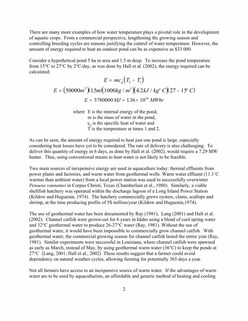
There are many more examples of how water temperature plays a pivotal role in the developmentof aquatic crops. From a commercial perspective, lengthening the growing season and controlling breeding cycles are reasons justifying the control of water temperature. However, theamount of energy required to heat an outdoor pond can be as expensive as $33 000.

Consider a hypothetical pond 5 ha in area and 1.5 m deep. To increase the pond temperaturefrom 15°C to 27°C by 2°C/day, as was done by Hall et al. (2002), the energy required can becalculated:

( )E mc T Tp= −2 1

( )( )( )( )( )E m m kg m kJ kg C C= ° − °50000 15 1000 4 2 27 152 3. / . /

E MJ MWhr= = ×3780000 136 1010.

where E is the internal energy of the pond,m is the mass of water in the pond, cp is the specific heat of water and T is the temperature at times 1 and 2.

As can be seen, the amount of energy required to heat just one pond is large, especiallyconsidering heat losses have yet to be considered. The rate of delivery is also challenging. Todeliver this quantity of energy in 6 days, as done by Hall et al. (2002), would require a 7.29 MWheater. Thus, using conventional means to heat water is not likely to be feasible.

Two main sources of inexpensive energy are used in aquaculture today: thermal effluents frompower plants and factories, and warm water from geothermal wells. Warm water effluent (11.1/Cwarmer than ambient water) from a local power station was used to successfully overwinterPenaeus vannamei in Corpus Christi, Texas (Chamberlain et al., 1980). Similarly, a viableshellfish hatchery was operated within the discharge lagoon of a Long Island Power Station(Kildow and Huguenin, 1974). The hatchery commercially grews oysters, clams, scallops andshrimp, at the time producing profits of 5$ million/year (Kildow and Huguenin,1974).

The use of geothermal water has been documented by Ray (1981), Lang (2001) and Hall et al.(2002). Channel catfish were grown-out for 6 years in Idaho using a blend of cool spring waterand 32°C geothermal water to produce 26-27°C water (Ray, 1981). Without the use ofgeothermal water, it would have been impossible to commercially grow channel catfish. Withgeothermal water, the commercial growing season for channel catfish lasted the entire year (Ray,1981). Similar experiments were successful in Louisiana, where channel catfish were spawnedas early as March, instead of May, by using geothermal warm water (36°C) to keep the ponds at27°C (Lang, 2001; Hall et al., 2002) These results suggest that a farmer could avoiddependency on natural weather cycles, allowing farming for potentially 365 days a year.

Not all farmers have access to an inexpensive source of warm water. If the advantages of warmwater are to be used by aquaculturists, an affordable and generic method of heating and cooling

3

water must be developed. The first step involves determining the energy load; how much energymust be supplied or removed from a pond to control its temperature? To do this, an energybalance must be performed.

Energy balances for bodies of water have been done before. Three cases in particular (solarponds, cooling ponds and winter waterways) are especially interesting because of the similaritiesbetween these ponds and aquaculture ponds.

• Solar ponds. Solar ponds are salt water ponds (salinity of 35%) which capture and storesolar energy. These ponds can be used for low temperature (90/C) heat applications (ex:heating water). (An excellent and extensive solar pond literature review with cross-references has been published (Kamal, 1991) Energy balances are done in these studies todetermine the pond performance with respect to varying amounts of solar radiation. However, the water in solar ponds does not move, whereas aquaculture pond water isoften mixed by aerators. Nonetheless, studies about these ponds have useful insightsabout energy balances in general.

• Cooling ponds. Cooling ponds are of interest to power plants which must return water tothe environment without added energy. Cooling ponds are also used in agriculture tocool livestock to relieve stress. Heat balances have been done for industrial coolingponds (Pawlina et al., 1977; Cheih and Verma,1978) and for agricultural cooling ponds(Husser, 2001) to see how quickly heat is dissipated. Collectively, these models providea wealth of information, especially concerning pond surface heat transfer phenomena.

• Winter waterways. Energy balances have been used to predict winter fog and ice breakson waterways in the winter (Miles and Carlson ,1984; Andres,1984). By applying anenergy balance, these studies were able to determine a heat transfer coefficient for thewater/ice surface.

Despite the numerous listed advantages of water temperature control, and despite all the researchdone on energy balances in other areas, an energy balance performed for aquaculture ponds wasnot found. Such an energy balance, as argued before, would identify dominant energy transfermechanisms and allow engineers to properly design temperature control systems for outdooraquaculture ponds. The same energy balance could be used as a management tool in maintainingdesired pond temperatures.

Such an energy balance was done for the warm water ponds at the Louisiana State UniversityAquaculture Research Station (see Chapter 2 for a description of the warm water ponds).

A review of the theory pertaining to energy transfer mechanisms allowed for the development ofa differential equation describing energy transfer and temperature changes in aquaculture ponds.To solve this non-linear first order differential equation, a FORTRAN computer model calledPHATR (Pond Heat And Temperature Regulation), which used the forth order Runge-Kuttanumerical method, was written and developed. Initial model runs for both heated and unheated

4

ponds revealed the model’s ability to predict pond temperature changes. The appropriate timestep was also determined. The model was refined by examining how different equationspredicting evaporation and surface convection affected the output data. The extinctioncoefficient for certain warm-water ponds was determined experimentally while the albedo forthese ponds was determined empirically.

The model’s sensitivity to errors in the input data was studied by running the model severaltimes, using hypothetical weather data, while varying one of the parameters of interest. Theparameters of interest were average air temperature, solar radiation, wind speed and warm-waterflow rate.

Finally, management and design questions about the warm-water aquaculture ponds at the ARSwere addressed. PHATR was used to calculate the pond temperature throughout an averageweather year, the amount of energy needed to maintain the pond temperature constant at 15, 20,25, 30 and 35°C, the time it took to cool a 27°C pond on a cold winter night and the amount ofenergy required to warm a pond from 10 to 27°C during a typical January. Based on theresearch done for this document, improvements for the current ARS warm-water pond setupwere then suggested.

5

Road To the Farm OfficeTo the Warm Water Well

Discharge Ditch

12345678910111213

Ditch

17- Acre Lake North

Road To the Farm OfficeTo the Warm Water Well

Discharge Ditch

12345678910111213

Ditch

17- Acre Lake North

CHAPTER 2: DESCRIPTION OF THE WARM-WATER PONDS AND ITSINSTRUMENTATION

2.1 The Ponds

The geothermal warm water ponds, located at the LSU Agricultural Center AquacultureResearch Station (ARS) in Baton Rouge, Louisiana, were used as a reference for comparingcalculated results from energy balances with measured pond data. These ponds were also usedto experimentally obtain certain parameters for calculations.

Figure 2.1: There were twelve rectangular and one trapezoidal warm water ponds at the LSUAquaculture Research Station. Each pond had access to cool (21°C) and warm (36°C) water. Each rectangular pond was approximately 10 m by 30 m. The pond discharge pipes were at theSouth end where excess water was sent to the discharge ditch between the ponds and the road.

There were 13 clay earthen ponds (Figure 2.1). Twelve ponds were roughly 10 meters by 30meters (Figure 2.2) and a 13th pond was a trapezoid (the dimensions of the ponds, as ofSeptember, 2002, are listed in Table 2.1). The pond bottom soil was classified as a SharkeyDundee clay.

Each pond had access to warm geothermal water (36°C) and cold well water (21°C). Each pond hada discharge pipe which maintained the pond depth at 1.22 m. An aerator (Power House, 3/4 hp) was

6

Outlet

Aerator

Inlet

Figure 2.3: The general layout of a warmwater pond consisted of an aerator,approximately 2 m from the inlet, and adischarge pipe, approximately 28 m from theinlet. The pond dimensions were roughly 30m x 10 m. The water column was maintainedat 1.22 m..

Figure 2.2: Pond 6, shown here, faced North towards the 17-Acre Lake (shown in back).The pond was equipped with an aerator and inlet valves for cold and warm water. Thedischarge pipe was at the South end of the pond. Floats marked the location of spawningcans on the pond bottom. An anemometer was installed to measure wind speed. Alsopresent were thermocouples, measuring the pond temperature at 0, 2.5, 5 and 10 cmbelow the water surface.

17 Acre LakeInlet valves

Aerator

Float

Anemometer

Discharge Pipe

Thermocouple Float

7

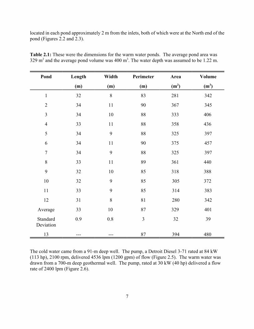
located in each pond approximately 2 m from the inlets, both of which were at the North end of thepond (Figures 2.2 and 2.3).

Table 2.1: These were the dimensions for the warm water ponds. The average pond area was329 m2 and the average pond volume was 400 m3. The water depth was assumed to be 1.22 m.

Pond Length Width Perimeter Area Volume

(m) (m) (m) (m2) (m3)

1 32 8 83 281 342

2 34 11 90 367 345

3 34 10 88 333 406

4 33 11 88 358 436

5 34 9 88 325 397

6 34 11 90 375 457

7 34 9 88 325 397

8 33 11 89 361 440

9 32 10 85 318 388

10 32 9 85 305 372

11 33 9 85 314 383

12 31 8 81 280 342

Average 33 10 87 329 401

StandardDeviation

0.9 0.8 3 32 39

13 --- --- 87 394 480

The cold water came from a 91-m deep well. The pump, a Detroit Diesel 3-71 rated at 84 kW(113 hp), 2100 rpm, delivered 4536 lpm (1200 gpm) of flow (Figure 2.5). The warm water wasdrawn from a 700-m deep geothermal well. The pump, rated at 30 kW (40 hp) delivered a flowrate of 2400 lpm (Figure 2.6).

8

Figure 2.4: This Detroit Diesel well, rated at 113 hp,supplied cold 21°C water to the warm water ponds. The wellwas 91 m deep.

Figure 2.5: This pump, rated at 30 kW,supplied warm water (36°C) to the warm waterponds. The well was 700 m deep.

9

Figure 2.6: The data logger (a) was used to automatically open and close a ball valve (b)with the use of an actuator. The ball valve controls the flow of warm geothermal water.Submerged thermocouples located roughly 20 m from the inlet sent signals to the datalogger. The data logger processed the signals: if the pond temperature was too cold, theautomatic valve opened. If the pond was too warm, the valve closed.

(b)(a)

2.2 The Instrumentation

The pond temperature was regulated with the use of a solenoid ball valve connected to aCampbell Scientific CR 23X data logger (Campbell Scientific Inc., North Logan, UT). Inresponse to low temperatures automatically measured with a type T (copper-constantan)thermocouple, a signal, sent from the data logger, opened the solenoid valve, allowing warmwater to flow into the pond. Once the desired temperature was attained, the valve was closeduntil the pond cooled to the minimum set temperature. Below this point, the valve was againopened. Hall et al. (2002) described in greater detail the control system. When inducingspawning in channel catfish, the pond temperature was maintained between 26°C and 27°C.

Campbell Scientific 21X data loggers (Campbell Scientific Inc., North Logan, UT) measured thepond temperature in locations described in Table 2.2.

Using these ponds and this instrumentation as a reference, calculated results from a theoreticalenergy balance were validated.

10

Table 2.2: This is the location log for all the Campbell Scientific 21X data loggers used. Each datalogger was assigned a letter for identification purposes. Two data loggers, Ca and D, were replacedover an 18 month period. Each data logger had 8 channels (Channels 1 through 9) devoted tomeasuring temperature. Thermocouples (TC) were located either within a meter of the aerator, ameter from the discharge pipe, or approximately in the middle of the pond. Different configurationswere used to measure different temperature profile with respect to depth (see Table 2.3 for moredetails about the configuration).

Dates Pond Data logger Channels Location of TC Configuration

2/19/02 to 03/20/02 9 A 6, 7, 8, 9 Aerator 1

2/19/02 to 03/20/02 9 B 6, 7, 8, 9 Middle 1

2/19/02 to 03/20/02 9 C 6, 7, 8, 9 Discharge 1

2/19/02 to 03/20/02 10 A 2, 3, 4, 5 Aerator 1

2/19/02 to 03/20/02 10 B 2, 3, 4, 5 Middle 1

2/19/02 to 03/20/02 10 C 2, 3, 4, 5 Discharge 1

2/19/02 to 03/20/02 11 D 6, 7, 8, 9 Aerator 1

2/19/02 to 03/20/02 11 E 6, 7, 8, 9 Middle 1

2/19/02 to 03/20/02 11 F 6, 7, 8, 9 Discharge 1

2/19/02 to 03/20/02 12 D 2, 3, 4, 5 Aerator 1

2/19/02 to 03/20/02 12 E 2, 3, 4, 5 Middle 1

2/19/02 to 03/20/02 12 F 2, 3, 4, 5 Discharge 1

4/02/02 to 05/11/02 5 A 6, 7, 8, 9 Aerator 1

4/02/02 to 05/11/02 5 B 6, 7, 8, 9 Middle 1

4/02/02 to 05/11/02 5 C 6, 7, 8, 9 Discharge 1

4/02/02 to 05/11/02 6 A 2, 3, 4, 5 Aerator 1

4/02/02 to 05/11/02 6 B 2, 3, 4, 5 Middle 1

4/02/02 to 05/11/02 6 C 2, 3, 4, 5 Discharge 1

4/02/02 to 05/11/02 7 D 6, 7, 8, 9 Aerator 1

4/02/02 to 05/11/02 7 E 6, 7, 8, 9 Middle 1

4/02/02 to 05/11/02 7 F 6, 7, 8, 9 Discharge 1

11

Table 2.2 Continued

Dates Pond Data logger Channels Location of TC Configuration

4/02/02 to 05/11/02 8 D 2, 3, 4, 5 Aerator 1

4/02/02 to 05/11/02 8 E 2, 3, 4, 5 Middle 1

4/02/02 to 05/11/02 8 F 2, 3, 4, 5 Discharge 1

05/11/02 to 06/25/02 1 D 6, 7, 8, 9 Aerator 1

05/11/02 to 06/25/02 1 B 6, 7, 8, 9 Middle 1

05/11/02 to 06/25/02 1 A 6, 7, 8, 9 Discharge 1

05/11/02 to 06/25/02 2 D 2, 3, 4, 5 Aerator 1

05/11/02 to 06/25/02 2 B 2, 3, 4, 5 Middle 1

05/11/02 to 06/25/02 2 A 2, 3, 4, 5 Discharge 1

05/11/02 to 06/25/02 3 E 6, 7, 8, 9 Aerator 1

05/11/02 to 06/25/02 3 H 6, 7, 8, 9 Middle 1

05/11/02 to 06/25/02 3 F 6, 7, 8, 9 Discharge 1

05/11/02 to 06/25/02 4 E 2, 3, 4, 5 Aerator 1

05/11/02 to 06/25/02 4 H 2, 3, 4, 5 Middle 1

05/11/02 to 06/25/02 4 F 2, 3, 4, 5 Discharge 1

10/07/02 to 11/02/02 7 A all Aerator 2

10/07/02 to 11/02/02 7 D all Middle 2

10/07/02 to 11/02/02 7 H all Discharge 2

10/07/02 to 01/24/03 13 E all Aerator 2

10/07/02 to 01/24/03 13 F all Middle 2

10/07/02 to 01/24/03 13 B all Discharge 2

11/08/02 to 01/24/03 13 H all Aerator 3

11/08/02 to 01/24/03 13 A all Middle 3

11/08/02 to 01/24/03 13 G all Discharge 3

12

Table 2.2 Continued

Dates Pond Data logger Channels Location of TC Configuration

02/12/03 to 03/28/03 9 E all Aerator 4

02/12/03 to 03/28/03 9 F all Discharge 4

02/12/03 to 03/28/03 12 H all Aerator 4

02/12/03 to 03/28/03 12 A all Discharge 4

02/12/03 to 03/28/03 3 G all Aerator 4

02/12/03 to 03/28/03 3 B all Discharge 4

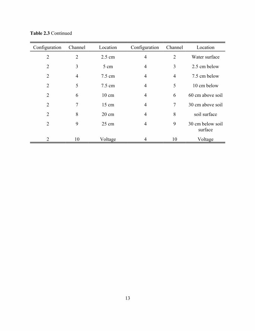
Table 2.3: These thermocouple configurations were used to measure the temperature profile withinthe water column. The channel refers to the data logger space where the information was stored.Location refers to the thermocouple location within the water column. The “reference” locationrefers to the reference thermocouple inside the data logger. The “voltage” location refers to thechannel which recorded the data logger voltage. The thermocouple locations in Configuration 1were not measured. All measurements in Configuration 2 were below the pond bottom - soilsurface. All measurements in Configuration 3 were below the water surface.

Configuration Channel Location Configuration Channel Location

1 1 Reference 3 1 Reference

1 2 Soil 3 2 0 cm

1 3 Bottom 3 3 2.5 cm

1 4 Top 3 4 5 cm

1 5 Surface 3 5 7.5 cm

1 6 Soil 3 6 10 cm

1 7 Bottom 3 7 12.5 cm

1 8 Top 3 8 15 cm

1 9 Surface 3 9 20 cm

1 10 Voltage 3 10 Voltage

2 1 0 cm 4 1 Reference

13

Table 2.3 Continued

Configuration Channel Location Configuration Channel Location

2 2 2.5 cm 4 2 Water surface

2 3 5 cm 4 3 2.5 cm below

2 4 7.5 cm 4 4 7.5 cm below

2 5 7.5 cm 4 5 10 cm below

2 6 10 cm 4 6 60 cm above soil

2 7 15 cm 4 7 30 cm above soil

2 8 20 cm 4 8 soil surface

2 9 25 cm 4 9 30 cm below soilsurface

2 10 Voltage 4 10 Voltage

14

CHAPTER 3: THEORY

The theory used to develop an energy balance for outdoor aquaculture ponds is presented in thischapter.

3.1 Definitions

3.1.1 Energy and Heat

Although the terms energy and heat may be used interchangeably in everyday language, bothterms are thermodynamically different. Obert (1949) gave the following definition of energy:

“Energy is broadly defined as the ability to produce a change from the existing conditions.”

Energy exists in various forms: kinetic, potential, internal, etc. Because one can consider a pondto have no kinetic or potential energy, a pond simply has internal energy, which was defined byAmerican Society of Heating, Refrigerating and Air-conditioning (ASHRAE) (Anonymous,1985) as:

“The energy possessed by a system caused by the motion of the molecules and/or intermolecular forces.”

Heat, on the other hand, should be considered as energy in transit. ASHRAE (1985) defined heatas:

“the mechanism that transfers energy across the boundary of systems with differing temperatures, always in the direction of the lower temperature.”

to which Obert (1949) would have added:

“Heat is technically a term reserved for transfers of energy where the driving factor (potential) is a temperature difference across a system boundary. It is wrong under this definition to speak of heat contained in a body; the correct term is internal energy.”

Therefore, for the purposes of this study, a pond has internal energy and heat is the energy beingexchanged between the pond and the surroundings.

3.1.2 The Principle Behind the Heat Balance

The conventional method of performing a heat balance requires the definition of a control

15

(3.1)

(3.2)

volume. Therefore, for this study, all liquid water in the pond was defined as the control volumeand Epond was the amount of energy within its boundaries. The amount of internal energy insidethe control volume can be calculated at any time as:

where D is the density of the water (kg/m3),� is the volume of water in the pond, cp is the specific heat of water (kJ/kg/C) andT is the temperature (/C).

It is assumed that the pond is sufficiently mixed so that the temperature throughout the pond isapproximately the same (see Appendix 1). In the event where this is not the case (for instance,when thermal layering occurs), the total energy in the pond is the sum of the energy in the twolayers, or:

Because the temperature and occasionally the volume of the water changes over time, the amountof energy within the control volume also changes, as described by the following equation:

These changes are caused in part by:

• the absorbtion of solar radiation by the water, • the exchange of heat with the soil, primarily due to conduction, • heat exchanges with the air, due to convection, evaporation and back radiation, • the bulk movement of water (and thus the bulk transport of energy) across the

control system boundary.

All these vectors of heat movement can be quantified and balanced with the rate at which theenergy within the system is changing. (This is the principle behind the heat balance.) Figure 3.1schematically represents the following mathematical expression:

where E is the total energy at any given time (t) in the pond, qsolar is the rate of energy gained by the pond by radiation

(3.3)

(3.4)

16

Figure 3.1: Each arrow in this schematic of an energy balance centered around a pond representsan energy transfer mechanism (energy vector) which must be accounted for when determining therate at which energy is stored in the pond. Vectors considered minor and not shown in this diagramare the absorption of light by chlorophyll, energy losses through seepage and light reflected by thesuspended particles in the pond.

qback is the rate of heat exchanged due to back radiation qsky is the long wave radiation from the sky, qevap is the rate of heat lost through the evaporation of water qconv is the rate of heat exchanged with the air by convection qsoil is the rate of heat exchanged with the soil qseep is the rate of bulk energy lost through seepage qrain is the rate of bulk energy gained due to rainfall qwell is the rate of bulk energy gained from the warm water well qout is the rate of bulk energy lost to the overflow of waterqother is the rate of energy transfer from or to other sources.

Note that individual heat transfer components can be either positive or negative, depending onwhether energy is entering or leaving the system. In order to avoid confusion, energy enteringthe system will be considered positive (heat gain) while energy exiting the system will be treatedas negative (heat loss).

17

(3.5)

(3.6)

3.2 Heat Transfer through Radiation (qsolar, qbackrad,qsky)

3.2.1. Definition of Thermal Radiation

Radiation, in general, can be viewed as the propagation of energy in the form of electromagneticwaves (classical approach) or discrete photons (quantum-mechanics approach). No medium isrequired in its propagation (Holman, 1997). Although there are many different kinds ofradiation, for the purposes of this study, only thermal radiation (with wavelengths ranging from8=0.2 to 1000 :m) will be considered and all usage of the term radiation will refer to thermalradiation.

For black and grey bodies, the amount of energy being propagated by radiation is dependant onthe absolute temperature of the emitter. The general relationship quantifying heat transferred dueto radiation, for a grey body, is:

where q is the heat transfer rate (W), g is the emissivity of the grey body (fraction)F is the Stefan-Boltzmann constant (5.67 x 10-8 W/m2/K4)T is the temperature of the grey body (K)

For outdoor aquaculture ponds, two types of radiation must be considered: short wave and longwave radiation. Short wave radiation has more energy than long wave radiation, due to thefollowing relationship:

where Equantum is the energy within a quantumhPlanck is Planck’s constant (6.625 x 10-34 J s)< is the radiation frequency (s-1)c is the speed of light (-3 x 10-8 m/s in a vacuum)

8 is the radiation wavelength (m)

This becomes important when considering the transmittance of radiation through media like theatmosphere or water.

3.2.2 Shortwave Radiation

3.2.2.1 Laws of Reflection and Refraction

When a beam goes from one medium to an other, as is shown in Figure 3.2, two phenomenaoccur: either the beam is reflected or refracted. Consider a beam striking a surface with an angle

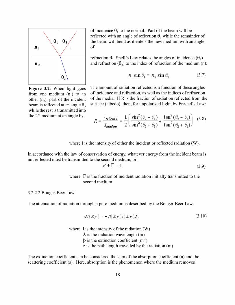
18

(3.7)

Figure 3.2: When light goesfrom one medium (n1) to another (n2), part of the incidentbeam is reflected at an angle 23

while the rest is transmitted intothe 2nd medium at an angle 22.

of incidence 21 to the normal. Part of the beam will bereflected with an angle of reflection 21 while the remainder ofthe beam will bend as it enters the new medium with an angleof

refraction 22. Snell’s Law relates the angles of incidence (21)and refraction (22) to the index of refraction of the medium (n):

The amount of radiation reflected is a function of these anglesof incidence and refraction, as well as the indices of refractionof the media. If R is the fraction of radiation reflected from thesurface (albedo), then, for unpolarized light, by Fresnel’s Law:

where I is the intensity of either the incident or reflected radiation (W).

In accordance with the law of conservation of energy, whatever energy from the incident beam isnot reflected must be transmitted to the second medium, or:

where ' is the fraction of incident radiation initially transmitted to thesecond medium.

3.2.2.2 Bouger-Beer Law

The attenuation of radiation through a pure medium is described by the Bouger-Beer Law:

where I is the intensity of the radiation (W)8 is the radiation wavelength (m)$ is the extinction coefficient (m-1)z is the path length travelled by the radiation (m)

The extinction coefficient can be considered the sum of the absorption coefficient (a) and thescattering coefficient (s). Here, absorption is the phenomenon where the medium removes

(3.8)

(3.9)

(3.10)

19

energy from the radiation beam, causing the medium to gain more energy while reducing theintensity of the beam. Scattering, on the other hand, is the reflection of radiation by suspended

particles. For particles sizes with diameters much greater than the radiation wavelength, thescattering coefficient is (Siegel, 1981):

where r is the mean radius of the particleN is the number of particles per unit volume

Both the absorption and scattering coefficients are dependant on the wavelength and the pathtraveled by the radiation.

3.2.2.3. Solar Radiation (qsolar)

Radiation emitted by the Sun travels through the vacuum of space unaltered. Table 3.2 lists thepercentage of energy associated with certain bandwidths of solar radiation emitted from ablackbody at 5800K (the temperature of the sun - Holman, 1997).

Table 3.2: Assuming the sun was a black body with a surface temperature of 5800 K, the totalemitted energy for given bandwidths were calculated. 38.5% of all emitted energy is associated withthe visible spectrum.

Bandwidth (nm) Percentage of total emitted energy

under 0.2 0.1%0.2-0.3 3.5%0.3-0.4 6.9%0.4-0.5 14.3%0.5-0.6 12.2%0.6-0.7 12.0%0.7-0.8 9.0%0.8-0.9 8.0%0.9-1.0 6.0%1.0 -1.2 9.0%1.2 - 1.6 9.0%1.6 - 2.2 5.0%2.2 - 2.8 2.0%

above 2.8 3.0%

To determine the amount of incoming extraterrestrial radiation, the following equations can beused:

(3.11)

20

(3.15)

(3.16)

(3.17)

(3.18)

(3.19)

where J is an angle (radians) n is the day of the year (on January 1st , n = 1)R is the distance from the Earth to the sun (km)R0 is the mean distance from the Earth ot the sun, 1.496 x 108 kmD0 is the solar constant (1353 W/m2)Dx is the extra-terrestrial radiationR is a “clearness” factor (1 on clear days, 0.2 on cloudy days)

Upon entering the Earth’s atmosphere, the properties of this radiation change. Direct beamradiation, defined as solar radiation whose path has been unaltered by atmospheric scattering,changes intensity as atmospheric gases, such as ozone, water vapor and CO2, absorb specificwavelength bands of radiation. For instance, it is well known that the ozone layer absorbs UVlight. Water vapor and CO2 absorb infra-red radiation (Kondratyev, 1969). Solar radiation whichhas changed direction due to scattering is called diffuse radiation. Needless to say, diffuseradiation is also absorbed by atmospheric gases (probably more so due to its increased travelingdistance). Diffuse radiation, although it comes from all directions, can be considered like beamradiation incident to the Earth’s surface at 60/ (Duffie and Beckman, 1980). The solar radiationspectrum was measured by Threlkeld and Jordan (1958) and is shown in Figure 3.3.

The solar zenith (2z) is the angle formed by the pond normal and direct incident beam radiation(the angle of incidence in Figure 3.2), and this angle varies with the time of day, the time of year

and the geographical position of the pond. The solar zenith is given by the following equations(Anderson, 1983):

(3.12)

21

(3.15)

(3.13)

(3.14)

Figure 3.3: This is the solar spectrum. There is more energy in thevisible spectrum because the frequency of the radiation waves ishigher than waves in the infra-red spectrum. (Threlkeld and Jordan,1958).

Ttime = LST + (Lnt - Lng) ÷ 15

22

(3.22)

(3.23)

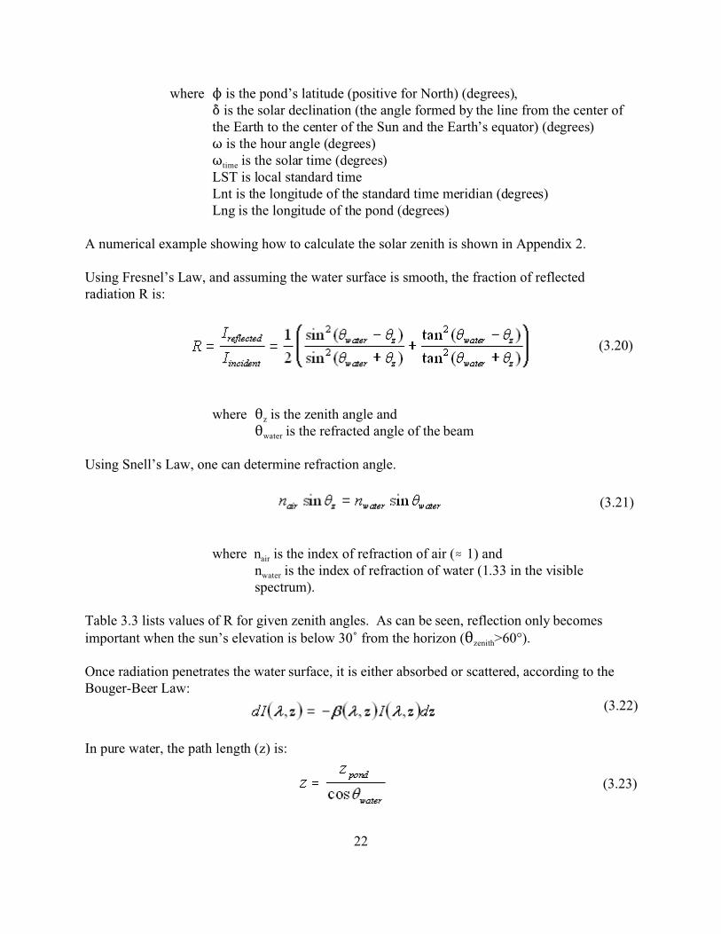
where N is the pond’s latitude (positive for North) (degrees), * is the solar declination (the angle formed by the line from the center ofthe Earth to the center of the Sun and the Earth’s equator) (degrees)T is the hour angle (degrees)Ttime is the solar time (degrees)LST is local standard timeLnt is the longitude of the standard time meridian (degrees)Lng is the longitude of the pond (degrees)

A numerical example showing how to calculate the solar zenith is shown in Appendix 2.

Using Fresnel’s Law, and assuming the water surface is smooth, the fraction of reflectedradiation R is:

where 2z is the zenith angle and2water is the refracted angle of the beam

Using Snell’s Law, one can determine refraction angle.

where nair is the index of refraction of air (. 1) and nwater is the index of refraction of water (1.33 in the visiblespectrum).

Table 3.3 lists values of R for given zenith angles. As can be seen, reflection only becomesimportant when the sun’s elevation is below 30/ from the horizon (2zenith>60°).

Once radiation penetrates the water surface, it is either absorbed or scattered, according to theBouger-Beer Law:

In pure water, the path length (z) is:

(3.21)

(3.20)

23

Table 3.3: The amount of light reflected at the water surface is dependant on the angle of incidence(the zenith angle). Using Fresnel’s Law, the following table was generated.

Zenith Angle (°) Reflection (%)

10 2.0

20 2.0

30 2.1

40 2.4

50 3.3

60 5.9

70 13.3

80 34.7

89 89.6

The absorption of light in pure water has been reviewed (Irvine and Pollack, 1968; Kondratyev,1969; Hale and Querry, 1973;Rabl and Nielsen, 1975; Tsilingiris, 1991). For shortwaveradiation, water is not a grey body and, as a result, its absorbance varies with the wavelength ofthe incident radiation. Results from the literature have been compiled to produce tablesdescribing the absoprtion coefficient of pure water as a function of the radiation wavelength (seeTable 3.4 and Figure 3.4) (Irvine and Pollack, 1968; Hale and Querry, 1973). Water poorlyabsorbs radiation in the ultra-violet and visible spectrums while being an excellent absorber ofinfra-red radiation, especially above 1200 nm. Kondratyev (1969) has tabulated the penetrationdepth of solar radiation through various thicknesses of water and his results are shown in Table3.5. Most of the solar radiation in the near infra-red spectrum is absorbed within the firstcentimeter of depth. Rabl and Nielsen (1975) determined that the radiation associated withwavelengths greater than 1200 nm represented 22.4% of the total incident radiation and thisradiation was totally absorbed in this upper water boundary layer. For radiation with 8< 1200nm, Rabl and Nielsen (1975) have developed the following approximation (to within 3%) todetermine the amount of radiation absorbed by water (qrad-1).

where qinc is the incident radiation upon the pond (W/m2)an is the absorption coefficient (cm-1)

(3.24)

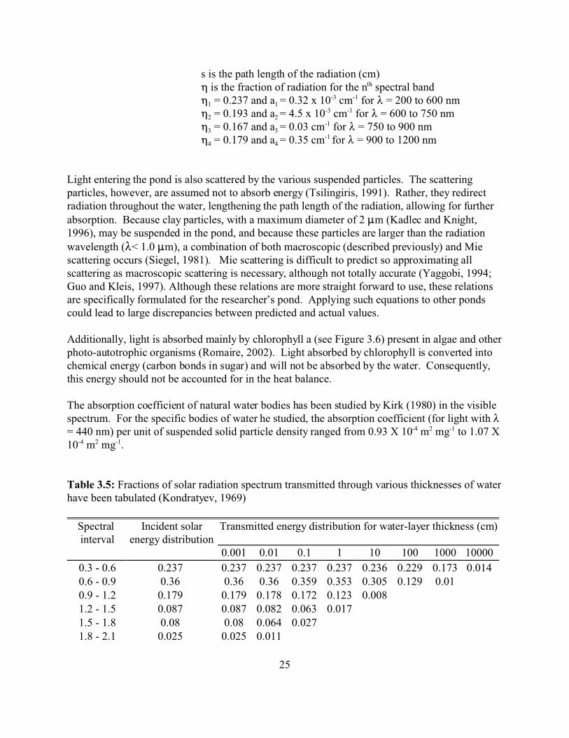
25

s is the path length of the radiation (cm)0 is the fraction of radiation for the nth spectral band01 = 0.237 and a1 = 0.32 x 10-3 cm-1 for 8 = 200 to 600 nm02 = 0.193 and a2 = 4.5 x 10-3 cm-1 for 8 = 600 to 750 nm03 = 0.167 and a3 = 0.03 cm-1 for 8 = 750 to 900 nm04 = 0.179 and a4 = 0.35 cm-1 for 8 = 900 to 1200 nm

Light entering the pond is also scattered by the various suspended particles. The scatteringparticles, however, are assumed not to absorb energy (Tsilingiris, 1991). Rather, they redirectradiation throughout the water, lengthening the path length of the radiation, allowing for furtherabsorption. Because clay particles, with a maximum diameter of 2 :m (Kadlec and Knight,1996), may be suspended in the pond, and because these particles are larger than the radiationwavelength (8< 1.0 :m), a combination of both macroscopic (described previously) and Miescattering occurs (Siegel, 1981). Mie scattering is difficult to predict so approximating allscattering as macroscopic scattering is necessary, although not totally accurate (Yaggobi, 1994;Guo and Kleis, 1997). Although these relations are more straight forward to use, these relationsare specifically formulated for the researcher’s pond. Applying such equations to other pondscould lead to large discrepancies between predicted and actual values.

Additionally, light is absorbed mainly by chlorophyll a (see Figure 3.6) present in algae and otherphoto-autotrophic organisms (Romaire, 2002). Light absorbed by chlorophyll is converted intochemical energy (carbon bonds in sugar) and will not be absorbed by the water. Consequently,this energy should not be accounted for in the heat balance.

The absorption coefficient of natural water bodies has been studied by Kirk (1980) in the visiblespectrum. For the specific bodies of water he studied, the absorption coefficient (for light with 8= 440 nm) per unit of suspended solid particle density ranged from 0.93 X 10-4 m2 mg-1 to 1.07 X10-4 m2 mg-1.

Table 3.5: Fractions of solar radiation spectrum transmitted through various thicknesses of waterhave been tabulated (Kondratyev, 1969)

Spectral interval

Incident solarenergy distribution

Transmitted energy distribution for water-layer thickness (cm)

0.001 0.01 0.1 1 10 100 1000 10000

0.3 - 0.6 0.237 0.237 0.237 0.237 0.237 0.236 0.229 0.173 0.014 0.6 - 0.9 0.36 0.36 0.36 0.359 0.353 0.305 0.129 0.01 0.9 - 1.2 0.179 0.179 0.178 0.172 0.123 0.008 1.2 - 1.5 0.087 0.087 0.082 0.063 0.017 1.5 - 1.8 0.08 0.08 0.064 0.027 1.8 - 2.1 0.025 0.025 0.011

30

2.1 - 2.4 0.025 0.025 0.019 0.001 2.4 - 2.7 0.007 0.006 0.002

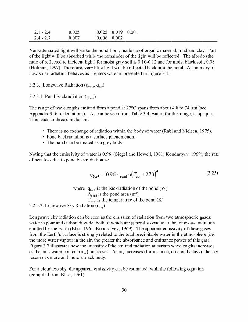
Non-attenuated light will strike the pond floor, made up of organic material, mud and clay. Partof the light will be absorbed while the remainder of the light will be reflected. The albedo (theratio of reflected to incident light) for moist gray soil is 0.10-0.12 and for moist black soil, 0.08(Holman, 1997). Therefore, very little light will be reflected back into the pond. A summary ofhow solar radiation behaves as it enters water is presented in Figure 3.4.

3.2.3. Longwave Radiation (qback, qsky)

3.2.3.1. Pond Backradiation (qback)

The range of wavelengths emitted from a pond at 27°C spans from about 4.8 to 74 :m (seeAppendix 3 for calculations). As can be seen from Table 3.4, water, for this range, is opaque. This leads to three conclusions:

• There is no exchange of radiation within the body of water (Rabl and Nielsen, 1975). • Pond backradiation is a surface phenomenon. • The pond can be treated as a grey body.

Noting that the emissivity of water is 0.96 (Siegel and Howell, 1981; Kondratyev, 1969), the rateof heat loss due to pond backradiation is:

where qback is the backradiation of the pond (W)Apond is the pond area (m2)Tpond is the temperature of the pond (K)

3.2.3.2. Longwave Sky Radiation (qsky)

Longwave sky radiation can be seen as the emission of radiation from two atmospheric gases:water vapour and carbon dioxide, both of which are generally opaque to the longwave radiationemitted by the Earth (Bliss, 1961, Kondratyev, 1969). The apparent emissivity of these gasesfrom the Earth’s surface is strongly related to the total precipitable water in the atmosphere (i.e.the more water vapour in the air, the greater the absorbance and emittance power of this gas). Figure 3.7 illustrates how the intensity of the emitted radiation at certain wavelengths increasesas the air’s water content (mw) increases. As mw increases (for instance, on cloudy days), the skyresembles more and more a black body.

For a cloudless sky, the apparent emissivity can be estimated with the following equation(compiled from Bliss, 1961):

(3.25)

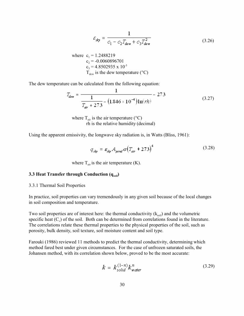
30

where c1 = 1.2488219 c2 = -0.0060896701

c3 = 4.8502935 x 10-5

Tdew is the dew temperature (°C)

The dew temperature can be calculated from the following equation:

where Tair is the air temperature (°C)rh is the relative humidity (decimal)

Using the apparent emissivity, the longwave sky radiation is, in Watts (Bliss, 1961):

where Tair is the air temperature (K).

3.3 Heat Transfer through Conduction (qsoil)

3.3.1 Thermal Soil Properties

In practice, soil properties can vary tremendously in any given soil because of the local changesin soil composition and temperature.

Two soil properties are of interest here: the thermal conductivity (ksoil) and the volumetricspecific heat (Cv) of the soil. Both can be determined from correlations found in the literature. The correlations relate these thermal properties to the physical properties of the soil, such asporosity, bulk density, soil texture, soil moisture content and soil type.

Farouki (1986) reviewed 11 methods to predict the thermal conductivity, determining whichmethod fared best under given circumstances. For the case of unfrozen saturated soils, theJohansen method, with its correlation shown below, proved to be the most accurate:

(3.26)

(3.27)

(3.28)

(3.29)

31

where ksolid is the thermal conductivity of the soil solids, kwater is the thermal conductivity of soilwater and n is the porosity of the soil (decimal). Changes in temperature could alter kwater

(ranging from 0.569 W/mK at 0/C to 0.598 W/mK at 27/C to 0.620 W/mK at 42/C), whichwould in turn affect the thermal conductivity of the soil. An average value for ksolid for Healy clayhas been determined by De Vries (1966) to be 2.5 W/mK.

The volumetric specific heat of soil (Cv) can be computed with the following relation (De Vries,1966):

where x is the soil fraction and C is the volumetric specific heat of each of the soil’s components: solids (s), water (w) and organic matter (org).

Table 3.7 is a list of values describing the thermal parameters of heavy soils in the literature.

Table 3.7 Presented here are thermal soil properties of interest found in the literature.

Soil k Cv Source Note(W/m K) (MJ/m3K)

Clay minerals 2.92 2 De Vries (1966) Property evaluated at 10/COrganic matter 0.25 2.51 De Vries (1966) Property evaluated at 10/CSilty clay loam 1.45-2.07 1.6-2.05 Sikora et al.(1990) Severely compacted soilSaturated clay 1.6 2.9 Kimball (1983) Soil has a porosity of 0.4.

Because the pond is lined with compacted heavy clay, in order to prevent leaks, these propertiesshould be fairly uniform. According to data presented by Sikora et al. (1990), compacted soils tendto have less variable thermal properties probably because less water and air is present in the soil.Despite the fact that the upper layer of the soil is composed mainly of organic mud, the liner wasassumed to be uniform. Furthermore, the pond liner can be assumed to be saturated with water,which removes the complications of gas-water mixtures in the soil. However, because the thermalproperties of water change with temperature, the soil’s properties too may be influenced bytemperature variations.

3.3.2 Heat Conduction in Soil

For soils, conduction was experimentally verified to be the predominant mode of heat transfer(Kimball et al, 1976). Consequently, the rate at which heat is exchanged with the soil (qsoil) can bedescribed by Fourier’s Law of heat conduction:

(3.31)

(3.30)

32

where k is the soil’s thermal conductivity (W/m K)A is the pond floor area (m2)T is the temperature of the soil (°C)z is the soil depth (m)(MT/Mz)*z=0 is the temperature gradient at the pond floor

The temperature gradient, in turn, can be determined from solutions to the heat diffusionequation:

If the propagation of heat is in the z direction only, then Equation 3.33 can be simplified to:

where t is time (s) " is the soil’s thermal diffussivity (m2/s).

If assumed constant, the thermal diffusivity can be calculated from other soil parameters:

where ksoil is the soil’s thermal conductivity (W/m/K) Dsoil is the soil’s bulk density (kg/m3)cp-soil is the soil’s specific heat (J/kg/K)Cv is the soil’s volumetric specific heat (J/m3/K).

To solve the heat diffusion equation, one initial and two boundary conditions are required. Forthe initial condition, it was assumed that the temperature throughout the entire soil was initiallythe same at all depths.

(3.32)

(3.33)

(3.34)

(3.35)

(3.36)

33

Since the liner can be treated as a semi-infinite solid (Van Wijk and De Vries,1966; Horton andWierenga,1983; Horton et al., 1983), the first boundary condition is

that is, at a very large depth, the soil’s temperature will not change. The other boundarycondition is dependent on the soil surface temperature. For the case where the water temperaturevaries diurnally, the second boundary condition is (Van Wijk and De Vries, 1966):

where Tavg is the average soil surface temperature for the period 1/T (°C) Tamp is half the total variation of the average temperature(°C)T is the frequency of the period being considered (s-1)

The resulting solution to the heat equation is (Van Wijk and De Vries, 1966):

where N is the phase constant for temperature variations at z = 0 m D is the dampening depth (m).

The dampening depth (D) is the depth where the variations in soil temperature are 1/e = 0.368times the temperature variations at the soil surface (example: if the daytime variation intemperature is 10/C at the surface, then at depth D, the temperature variation is 3.68/C). Thedampening depth is a function of the soil’s thermal properties as well as the period of variationconsidered (Van Wijk and De Vries, 1966):

where k is the thermal conductivity (W/m K), Cv is the soil’s volumetric specific heat (MJ/m3 K) and T is the period of the variation being considered (s).

Note that the dampening depth is o365 .19 times greater for annual variations than it is for dailyvariations. The daily dampening depth, according to Van Wijk and De Vries (1966) for saturatedclay is 12.2 cm and for an annual dampening depth, 233 cm.

(3.37)

(3.38)

(3.39)

(3.40)

34

The partial derivative of Equation 3.39, with respect to z, yields the temperature gradient for alldepths:

The temperature gradient at the soil surface (z = 0) is

This temperature gradient at the surface can be substituted into Fourier’s Law of heat conduction to finally determine the rate of heat transfer in the soil (qsoil):

For the case where the water temperature and the flow characteristics along the soil surfaceremain constant, the second boundary condition is:

where h is the heat transfer coefficient (W/m2/K).

Finding the heat transfer coefficient may prove difficult. An alternate second boundary conditioncould be:

The solution to the heat diffusion equation, with Equations 3.37 and 3.45 as boundary conditions,is (Holman, 1997):

(3.41)

(3.42)

(3.43)

(3.44)

(3.45)

35

where erf is the Gauss error function.

Taking the derivative with respect to z and substituting it into Fourier’s Law of heat conduction,the rate of heat exchange, at the surface (z=0), is:

3.4 Heat Transfer by Convection (qconv)

3.4.1 Newton’s Law of Cooling

Convection can be viewed as the combining heat transfer effects of conduction and advection influids. Heat transferred through convection can be calculated using Newton’s Law of cooling:

where qconv is the heat transferred by convection (W)h is the heat transfer coefficient (W/m2 K)A is the area of heat transfer (m2) Tsurface is the temperature of the surface (/C or K)Tfluid is the temperature of the cooling (or heating) fluid (/C or K).

For ponds, convection occurs in two places, the soil-water interface and the water-air interface. As already discussed in section 3.3.2, the rate of energy exchanged between the liner and thepond can be estimated by either Equation 3.43, 3.47 or 3.48 . For the water-air interface,convection is the only mode of heat transfer.

3.4.2 Determination of a Heat Transfer Coefficient - Nusselt Number Correlations

Nusselt number (Nu) correlations are traditionally used to predict a heat transfer coefficient,depending on:

• the geometry of the surface • the properties of the cooling fluid • the velocity at which the cooling fluid is moving

However, there seems to be no Nusselt number correlations in the literature for bodies of water

(3.46)

(3.47)

(3.48)

36

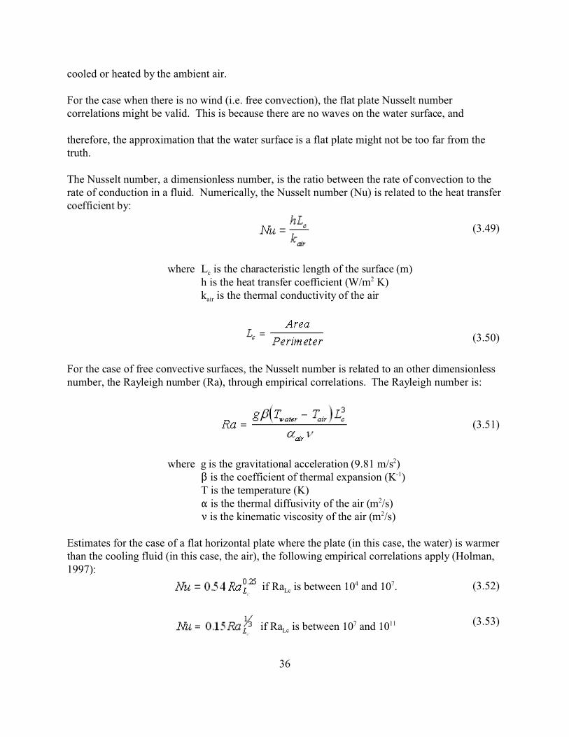
cooled or heated by the ambient air.

For the case when there is no wind (i.e. free convection), the flat plate Nusselt numbercorrelations might be valid. This is because there are no waves on the water surface, and

therefore, the approximation that the water surface is a flat plate might not be too far from thetruth.

The Nusselt number, a dimensionless number, is the ratio between the rate of convection to therate of conduction in a fluid. Numerically, the Nusselt number (Nu) is related to the heat transfercoefficient by:

where Lc is the characteristic length of the surface (m)h is the heat transfer coefficient (W/m2 K)kair is the thermal conductivity of the air

For the case of free convective surfaces, the Nusselt number is related to an other dimensionlessnumber, the Rayleigh number (Ra), through empirical correlations. The Rayleigh number is:

where g is the gravitational acceleration (9.81 m/s2)$ is the coefficient of thermal expansion (K-1) T is the temperature (K)" is the thermal diffusivity of the air (m2/s) < is the kinematic viscosity of the air (m2/s)

Estimates for the case of a flat horizontal plate where the plate (in this case, the water) is warmerthan the cooling fluid (in this case, the air), the following empirical correlations apply (Holman,1997):

if RaLc is between 104 and 107.

if RaLc is between 107 and 1011

(3.49)

(3.50)

(3.51)

(3.52)

(3.53)

37

If the plate is cooler than the fluid, and Ra is between 105 and 1010, then

For cases where wind is present (i.e. forced convection), different flat plate correlations could beused but run the risk of not being appropriate. Under windy conditions, the pond surface is nolonger flat because of waves. However, in the absence of any other relationship, the followingNusselt number correlation for mixed laminar and turbulent flow regions (for 5 x 105 < Re < 108)can be used (Holman, 1997):

where x is the length in the direction of wind flow Re is the Reynold’s numberPr is the Prandtl number

The previous equation is valid for Prandtl numbers between 0.6 to 60. The Reynold’s number,Re, is a dimensionless number representing the ratio of inertial to viscous forces in the boundarylayer of the fluid. It can be calculated as follows:

where Dair is the density of the air(kg/m3)V is the velocity of the air (m/s) :air is the dynamic viscosity of the air (kg/m s).

The Prandtl number, Pr, is a dimensionless number representing the ratio of the ability of a fluidto diffuse momentum to that of heat. It can be calculated as follows:

where < is the kinematic viscosity of the fluid (m2/s).

3.4.3 Determination of a Heat Transfer Coefficient - Direct Correlations

Other empirical equations have been used in the literature to estimate the heat transfer coefficientfor solar ponds, relating the heat transfer coefficient to wind speed (Duffie and Beckman, 1980,

(3.54)

(3.55)

(3.56)

(3.57)

38

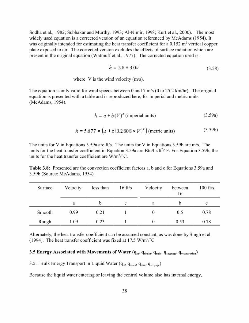
Sodha et al., 1982; Subhakar and Murthy, 1993; Al-Nimir, 1998; Kurt et al., 2000). The mostwidely used equation is a corrected version of an equation referenced by McAdams (1954). Itwas originally intended for estimating the heat transfer coefficient for a 0.152 m2 vertical copperplate exposed to air. The corrected version excludes the effects of surface radiation which arepresent in the original equation (Watmuff et al., 1977). The corrected equation used is:

where V is the wind velocity (m/s).

The equation is only valid for wind speeds between 0 and 7 m/s (0 to 25.2 km/hr). The originalequation is presented with a table and is reproduced here, for imperial and metric units(McAdams, 1954).

(imperial units)

(metric units)

The units for V in Equations 3.59a are ft/s. The units for V in Equations 3.59b are m/s. Theunits for the heat transfer coefficient in Equation 3.59a are Btu/hr/ft2/°F. For Equation 3.59b, theunits for the heat transfer coefficient are W/m2/°C.

Table 3.8: Presented are the convection coefficient factors a, b and c for Equations 3.59a and3.59b (Source: McAdams, 1954).

Surface Velocity less than 16 ft/s Velocity between16

100 ft/s

a b c a b c

Smooth 0.99 0.21 1 0 0.5 0.78

Rough 1.09 0.23 1 0 0.53 0.78

Alternately, the heat transfer coefficient can be assumed constant, as was done by Singh et al.(1994). The heat transfer coefficient was fixed at 17.5 W/m2//C

3.5 Energy Associated with Movements of Water (qin, qdrain, qrain, qseepage, qevaporation)

3.5.1 Bulk Energy Transport in Liquid Water (qin, qdrain, qrain, qseepage)

Because the liquid water entering or leaving the control volume also has internal energy,

(3.58)

(3.59a)

(3.59b)

39

movements of liquid water across the system boundary represent gains or losses of energy. Therate of bulk energy moved across the system boundary can be calculated with the followingequation:

where m’ is the mass flow rate of water into (or out of) the system, cp is the specific heat of water and T is the temperature of the water.

When considering seepage, energy losses may be assumed small with respect to other heattransfer mechanisms because of the small infiltration flow rate. To validate this assumption,consider Darcy’s Equation, which states that the rate of seepage (m’seepage) is:

where khyd is the hydraulic conductivity (m/s), i is the hydraulic gradient (dimensionless) A is the pond floor area (m2).

For saturated clays, khyd can vary from 10-11 to 10-6 cm/s (Carbeneau, 2000) and i = 0.01(Cedergren, 1966). Therefore, for every square meter of pond area, 10-15 to 10-10 m3/s/m2 (or 10-9

to 10-4 mL/s/m2 = 8.64 x 10-5 to 8.64 mL/day/m2) of water are lost. As a result, it was assumedthat water infiltration, being so small, is negligible in the transport of energy (i.e. qseepage= 0) forideal conditions. This may not necessarily be true in the case of ponds where various animals(ex: crawfish, nutria, muskrats) dig tunnels through the levees. In such cases, water lossesthrough leaks may be considerable (even dangerous for the levee in some cases). Unfortunately,it is impossible to predict how much water (or energy) will flow through an animal’s tunnelsystem.

3.5.2 Latent Heat Loss (qevap)

The process of evaporation requires a lot of energy. Evaporation heat losses (qevap) are calculatedwith the following set of equations (Anonymous, 1992):

where m’evap is the rate of evaporation (kg/s)

(3.60)

(3.61)

(3.62)

(3.63)

40

hfg is the latent heat of vaporization (J/kg)E0 is the volumetric rate of evaporation (m3/s) Dwater is the density of water (kg/m3)T is the water temperature (°C).

The difference in water vapor pressure between the water surface and the air vapor pressure is thedriving force behind evaporation (Penman, 1948). The following equation is Dalton’s Law andmany equations used to predict evaporation have the same form:

where f(x) is an experimentally determined function, based on externalparameterspwater is the saturated liquid vapor pressure of the liquid waterpair is the partial pressure of water vapor in the air.

The diffusion of water vapor from the pond can be determined with the use of Fick’s Law, whichuses the same concept of vapor pressure differences as the driving force behind evaporation:

where D is the diffusion coefficient (m2/s)(for water diffusing into air at 25/C, D = 0.28 X 10-4 m2/s)A is the area of the pond (m2)Cwater is the water vapour concentration in the air (kg/m3)z is the distance above the water surface (m)MCwater/Mz is the concentration gradient of water vapor in the zdirection (above the water surface).

Water vapor can be considered an ideal gas, and because of this, Fick’s Law can be rewritten as afunction of partial pressures, rather than concentration.

where MM is the molar mass of water vapor (18 kg/mol)R0 is the universal gas constant (8314 J/mol K)T is the temperature of the water vapor (K) pvp is the vapor pressure (Pa).

(3.64)

(3.65)

(3.66)

41

Although all the values in Fick’s Law are known, the diffusion coefficient (D) might not betotally accurate when considering ponds exposed to wind (Holman, 1997). Whenever possible,experimental correlations should be developed and used (Holman, 1997; Pierahita, 1991).

Empirical equations specifically developed for bodies of water have been developed. One suchequation is (Penman, 1948):

where Eo is the evaporation rate (m3/s)V2 is the wind velocity at two meters above the surface (miles perday)psat-ws is the saturated vapor pressure of the water surface, evaluatedat the surface water temperature (Pa) pvp is the vapor pressure of the air (Pa).

The vapor pressure (pvp), (Anonymous, 1985), is:

where pvp-sat is the saturated vapor pressure of the air (Pa)N is the relative humidity (decimal)

The saturated vapor pressure of the water surface or the water vapor can be calculated using thefollowing equations from (Anonymous, 1985).

where T is the temperature of the water surface (K)C1 = -5800.2206C2=1.3914993 C3= -0.04860239 C4= 0.41764768x10-4

C5 = -0.14452093x10-7

C6 = 6.5459673

When determining the vapor pressure of the air, the saturated vapor pressure is evaluated for thecurrent air temperature.

Alternately, the following equation can be used to estimate the rate of evaporation (Piedrahita,

(3.67)

(3.68)

(3.69)

42

1991):

where E0 is the rate of evaporation (m3/s)A is the pond area (m2), V2 is the wind velocity 2 meters above the pond surface (km/h)psat-ws is the saturated vapor pressure (Pa)pvp is the air vapor pressure (Pa)

The Lake Hefner Equation is yet another equation which predicts evaporation (Anonymous,1952):

where E0 is the evaporation rate (in/day)V13ft is the wind speed recorded at 13 feet (mph)psat-ws is the saturated vapor pressure (in Hg)pvp is the air vapor pressure (in Hg)

A metric version of Equation 3.71

where E0 is the evaporation rate (m/s)u4m is the wind speed recorded at 4 meters (m/s)psat-ws is the saturated vapor pressure (Pa)pvp is the air vapor pressure (Pa)

In order to determine the wind speed at any height, the following equation can be used:

where u is the wind speed at either height x or y (feet)

As can be seen from Equation 3.71, the Lake Hefner Equation was designed for estimating dailyevaporation rates.

(3.70)

(3.71)

(3.72)

(3.73)

43

3.6 Other Sources of Energy

3.6.1 Pond Mud Respiration

Decomposition in pond muds may be a source of energy in aquaculture ponds. The energyreleased in pond muds is a byproduct of decomposer respiration (Boyd, 1995). Chemically, theaerobic respiration of glucose can be described with the following equation:

where )Hc is heat of combustion for glucose = 15.58 kJ/mol of glucose(Doran, 1995)

Semi-intensive aquaculture pond soils consume 1 to 2 gO2 /m2/day (or 0.03125 to 0.0625 molO2

/m2/day) while intensive aquaculture pond soils use 4 gO2 /m2/day (or 0.125 molO2 /m

2/day)(Boyd, 1995). Assuming that most of the generated energy does come from the combustion ofglucose, the total energy produced by decomposers in semi-intensive aquaculture pond soils is81.25 to 162.5 J/m2/day and in intensive aquaculture pond soils is 325 J/m2/day.

Factors which may cause variations in the rate of pond mud respiration include temperature,oxygen availability, pH and nutrient availability (Boyd, 1995).

3.6.2 Work Done by the Aerator

The aerators used for the warm water ponds are brand name Power House Aerators, rated at 3/4 hp (746 Watts). The work done by the aerator on the pond represents an input of energy.

The presented theory was reviewed in order to develop an energy balance for an outdoor earthenaquaculture pond. The development of the energy balance will be presented in Chapter 4.

44

PondInfluent

Effluent

Back Radiation

Rain

Long wave sky Radiation

Cloud

Soil

Evaporation

Convection

Solar Radiation

Sun

PondInfluent

Effluent

Back Radiation

Rain

Long wave sky Radiation

Cloud

Soil

Evaporation

Convection

Solar Radiation

Sun

Figure 4.1: This figure (taken from Figure 3.1) is a conceptual representation of an energybalance for an aquaculture pond. Each arrow represents an energy vector (a term in Equation3.4). Two-headed arrows represent transport phenomena which either move energy into thepond (when the surroundings are warmer than the pond) or out of the pond (when thesurroundings are cooler than the pond). By taking the sum of all vectors, the rate of change forboth the pond’s internal energy and the pond temperature can be determined.

CHAPTER 4: THE CREATION OF A THEORETICAL COMPUTER MODEL

4.1 Introduction

Two models describing the rate of energy change in an aquaculture pond have been presented inChapter 3. The conceptual model (Figure 4.1) qualitatively describes how energy moves intoand out of a pond.

A second model, Equation 3.4, is the mathematical representation of Figure 4.1. This 1st ordernon-linear differential equation describes and quantifies each vector of energy transfer. Twodifferent solutions to Equation 3.4 are required for different types of circumstances:

• a steady state solution (dE/dt = 0): This solution quantifies energy vectors when the pondwater temperature, volume, specific heat and water density are constant. This includesthe case where the water temperature is held artificially high in the winter or artificiallylow in the summer.

45

• a transient solution (dE/dt…0): This solution is applicable when the water temperaturechanges either naturally or artificially.

Although the steady state solution will yield the “answer” to the initial problem (i.e. how muchenergy is required to heat or cool a pond), the transient solution is insightful because it:

• identifies when there is a surplus or deficit of internal energy in the pond • quantifies these surpluses and deficits, and • estimates the required power necessary to artificially change or maintain the water

temperature.

An analytical solution to Equation 3.4 is mathematically difficult to find, especially when thesystem is transient. For this reason, numerical methods have been used. The following chapteris a detailed description of PHATR (Pond Heating And Temperature Regulation), version 1.0, acomputer program used to numerically solve Equation 3.4.

4.2 Description of PHATR

PHATR was developed in FORTRAN, using the Essential Layhey FORTRAN 90 (ELF 90)compiler. It determines:

• the amount of energy being transferred through various transport mechanisms (i.e. thesize of each arrow - energy vector - in Figure 4.1)

• the predicted pond temperature

4.2.1 Equations Used to Solve Equation 3.4

Table 4.1 lists the equations for each of the terms in Equation 3.4 used by PHATR. Solarradiation, qsolar, is measured directly from field observations and is available to PHATR in a datafile.

4.2.2 Assumptions

These assumptions were used to simplify the solution of Equation 3.4.

• The water density and specific heat remained constant, despite changes in watertemperature. This was a reasonable assumption because at 0°C, the density 999.8 kg/m3

and at 43.3 °C, the density is 990.6 kg/m3 (less than 1% change). At 0°C, the specificheat is 4225 J/kg°C and at 43.3°C, the specific heat is 4174 J/kg/C (a relative change of1.2%) (Holman, 1997).

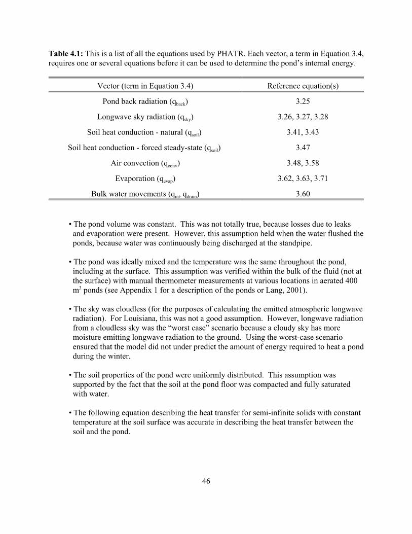
46

Table 4.1: This is a list of all the equations used by PHATR. Each vector, a term in Equation 3.4,requires one or several equations before it can be used to determine the pond’s internal energy.

Vector (term in Equation 3.4) Reference equation(s)

Pond back radiation (qback) 3.25

Longwave sky radiation (qsky) 3.26, 3.27, 3.28

Soil heat conduction - natural (qsoil) 3.41, 3.43

Soil heat conduction - forced steady-state (qsoil) 3.47

Air convection (qconv) 3.48, 3.58

Evaporation (qevap) 3.62, 3.63, 3.71

Bulk water movements (qin, qdrain) 3.60

• The pond volume was constant. This was not totally true, because losses due to leaksand evaporation were present. However, this assumption held when the water flushed theponds, because water was continuously being discharged at the standpipe.

• The pond was ideally mixed and the temperature was the same throughout the pond,including at the surface. This assumption was verified within the bulk of the fluid (not atthe surface) with manual thermometer measurements at various locations in aerated 400m3 ponds (see Appendix 1 for a description of the ponds or Lang, 2001).

• The sky was cloudless (for the purposes of calculating the emitted atmospheric longwaveradiation). For Louisiana, this was not a good assumption. However, longwave radiationfrom a cloudless sky was the “worst case” scenario because a cloudy sky has moremoisture emitting longwave radiation to the ground. Using the worst-case scenarioensured that the model did not under predict the amount of energy required to heat a pondduring the winter.

• The soil properties of the pond were uniformly distributed. This assumption wassupported by the fact that the soil at the pond floor was compacted and fully saturatedwith water.

• The following equation describing the heat transfer for semi-infinite solids with constanttemperature at the soil surface was accurate in describing the heat transfer between thesoil and the pond.

47

( )q

kA T T

tpond initial

0 =−

πα(Holman, 1997)

This assumption was reasonable if the following two conditions were satisfied:

• the considered time period (i.e. the time step) was small, which guaranteed thatthe soil could be considered as a semi-infinite solid.

• the Biot number was large. This assumption allowed for the use of a simplerboundary condition, as described in Appendix 4.

• There was no evaporation when the relative humidity of the air is at or above 100%.

• The Lake Hefner Equation (Equation 3.70) was accurate in predicting instantaneousevaporation .

• All incident solar radiation was absorbed by the water. This assumption was reasonablefor the following two reasons: • very little light was reflected at the pond surface (as shown in Table 3.3). • the water was turbid, preventing the escape of scattered solar radiation.

• All energy absorbed by the phytoplankton was transferred to the water, thus ignoring theamount of energy converted into sugars by chlorophyll.

• The decomposing microorganisms in the pond mud generated negligible amounts of heat.

• The aerators did negligible amounts of thermodynamic work. The amount of energyconverted from the work done by the mixing of the aerator to the internal energy of thepond was considered negligible.

4.2.3 Logic

PHATR followed these steps to determine the pond temperature:

1. Data input. PHATR initially acquired data from files. Such files contained information aboutthe weather (weather.dat), environmental constants and step sizes (information.dat) and the rateof water flow into the pond (flow.dat). For the special case where no warm water was flowinginto the pond (i.e. natural unforced pond water temperature), no file with information about theflow of warm water was required. The data were converted into the proper units.

2. Determination of coefficients. With the acquired data, PHATR proceeded to determine thecoefficients which did not depend on time or water temperature. Each mode of energy transferhad a coefficient term. Table 4.2 listed these coefficients.

(4.1)

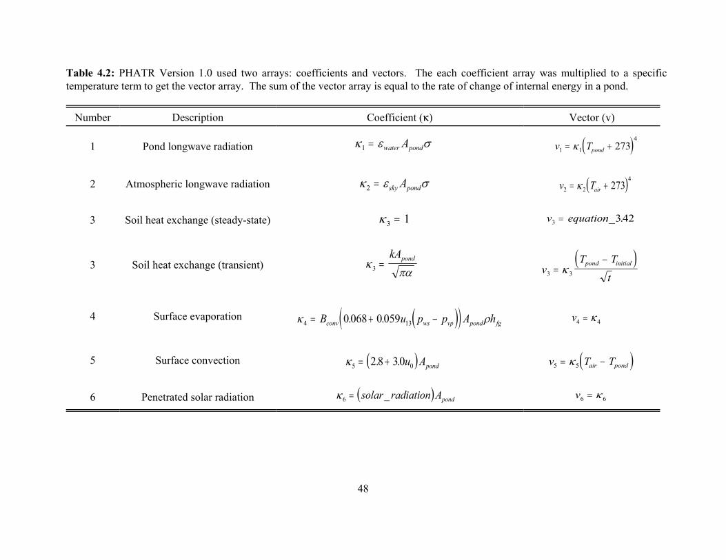
48

κ ε σ1 = water pondA ( )v Tpond1 1

4273= +κ

κ ε σ2 = sky pondA ( )v Tair2 2

4273= +κ

κ 3 1= v equation3 342= _ .

κπα3 =

kApond ( )v

T T

tpond initial

3 3=−

κ

( )( )κ ρ4 130 068 0 059= + −B u p p A hconv ws vp pond fg. . v4 4= κ

( )κ5 02 8 30= +. . u Apond ( )v T Tair pond5 5= −κ

( )κ 6 = solar radiation Apond_ v6 6= κ

Table 4.2: PHATR Version 1.0 used two arrays: coefficients and vectors. The each coefficient array was multiplied to a specifictemperature term to get the vector array. The sum of the vector array is equal to the rate of change of internal energy in a pond.

Number Description Coefficient (6) Vector (v)

1 Pond longwave radiation

2 Atmospheric longwave radiation

3 Soil heat exchange (steady-state)

3 Soil heat exchange (transient)

4 Surface evaporation

5 Surface convection

6 Penetrated solar radiation

49

(4.2)

(4.3)

(4.4)

(4.5)

(4.6)

(4.7)

(4.8)

3. Determination of vectors. The coefficients were then multiplied to the appropriate time orwater temperature term, the product being the vector term. The vector terms were “q”s inEquation 3.4 and arrows in Figure 4.1. Again, the formula for each vector term is given in Table4.2.

4. Determination of the “thermal mass”. The thermal mass is defined here as the energy requiredto raise the temperature of a given quantity of water by 1/C. The “thermal inertia” of the pond is:

ρ∀ pond pc

where D is the density of waterœpond is the pond volumecp is the specific heat of water

5. Solving Equation 3.4 - performing the energy balance. By substituting the vectors and thethermal mass into Equation 3.4, the rate of change of pond temperature is:

( )dTdt

qc

f t Tpond pond p

=

∀=

∑ρ

,

where T is the temperaturet is time q is an energy vector in Equation 3.4

To solve this differential equation, the 4th order Runge-Kutta numerical technique is used. The4th order Runge-Kutta numerical technique is recognized as an accurate method in evaluatingordinary differential equations. With the use of initial conditions, the Runge-Kutta techniqueevaluates the pond temperature with the following set of equations:

( ) ( )T t t T tF F F F

+ = ++ + +

∆ 1 2 3 42 26

( ) ( )F t f t T1 = ∆ ,

( )F t f tt

TF

21

2 2= + +

∆

∆,

( )F t f tt

TF

32

2 2= + +

∆

∆,

( ) ( )F t f t t T F4 3= + +∆ ∆ ,

50

6. Data output. The time, the vectors and the pond temperature were all recorded in an outputfile (output.dat). Steps 1 through 5 were repeated for the desired time period. Once the modelrun was completed, the output was analyzed with a spreadsheet program. An example of theoutput is in Figure 4.2.

4.3 Performance Tests for PHATR Version 1.0.

Tests were done to determine PHATR’s accuracy and stability for heated and unheated ponds. Model runs were compared to pond temperature data collected at the LSU Agriculture CenterAquaculture Research Station (ARS) warm water ponds (see Chapter 2). Each pond had oneaerator running continuously, access to warm water from the geothermal well (36°C) and coolwell water (21°C). The temperature was automatically controlled with an automated valve,actuated with a data logger (Campbell Scientific CR23X, Campbell Scientific Inc., North Logan,UT). The pond temperature was measured with a type T thermocouple 10 cm below the watersurface near the pond’s discharge and recorded with another data logger (Campbell ScientificCR23X, Campbell Scientific Inc., North Logan, UT).

Table 4.3 lists the dates and ponds chosen for performance tests.

Weather data used for the model runs were taken from the Louisiana Agriclimatic InformationWeb Site (www.lsuagcenter.com/weather) for the Ben Hur Weather Station, located less than akilometer away from the warm water ponds. Parameters of interest were air temperature, solarradiation, wind speed and relative humidity. The flow rate for each combination of open andclosed valves was measured by measuring the time it took to fill at 120 liter bucket. By knowingwhich combination of valves were open and closed, the flow rate at any time to any pond wasknown. The Campbell CR23X recorded when valves opened or closed.

By comparing the modeled data to the measured data, the model’s accuracy was measured withthree statistical parameters:

• the average bias: the bias is a measurement of how close the model is at estimating theactual pond temperature (i.e. the modeled temperature minus the measured temperature). The average bias is the average of all the biases at every time step.

• the standard deviation of the average bias: the standard deviation measures variations inthe bias. It is a good indicator of the model’s consistency (was the bias constant?) and itsability to predict changes in pond temperature.

• the correlation coefficient: the linear correlation coefficient - r- between the measuredand modeled temperatures is an other indicator of the model’s ability to predict changesin water temperature.

The time step for accuracy tests was 1 hour.

51

Time Pond Radiation Sky Radiation Soil Conduction Evaporation(seconds) (Watts) (Watts) (Watts) (Watts)31104000 -141134.256 102730.3863 27196.6768 -9104.06054931107600 -141007.1272 102584.9839 19712.36689 -8880.97218431111200 -140853.229 102697.6145 10997.06019 -8990.03361931114800 -140670.5473 101974.0129 1644.622574 -8367.49457731118400 -140450.5958 102213.4047 -7707.660745 -8670.23125231122000 -140201.3417 103100.8852 -16422.51511 -8589.58969631125600 -139930.1224 103635.1791 -23906.10567 -24428.7871831129200 -139533.3166 104149.6273 -29648.50621 -8143.50116331132800 -139292.2733 105663.5437 -33258.44981 -7474.269247

Convection Solar Radiation Pond Temperature(Watts) (Watts) (? C)

-15206.08307 0 11.82-15437.50172 0 11.75583932-14972.95103 0 11.67811036-16197.67802 0 11.58576104-15298.18691 0 11.47445165-14067.51148 0 11.34815519-27609.71635 394 11.21053757-12495.80442 17730.00079 11.00883595-11259.5179 49644.00079 10.88610036

Figure 4.2: This is an example fo the output file generated by PHATR Version 1.0. For every time step, thetime, the calculated value for each energy vector and the pond temperature were printed to an output file.

52

Table 4.3: Model runs were compared to the temperature data collected in these ponds at thesetimes.

Dates Pond Temperature Regime Performance Test

04/03/02 to 04/07/02 5, 6, 7, 8 Unheated Accuracy ofPHATR’s transientmode

11/09/02 to 12/16/02 13 Unheated Accuracy andstability of PHATR’stransient mode

12/25/02 to 1/24/03 13 Unheated Accuracy ofPHATR’s transientmode

02/13/03 to 03/23/03 3 Unheated Accuracy ofPHATR’s transientmode

02/13/03 to 03/23/03 9, 12 Heated (pondtemperature constant)

Accuracy andstability of PHATR’ssteady-state mode

Stability tests consisted of varying the time step used for a model run. Model runs with timesteps of 10 minutes, 30 minutes, 1 hour, 2 hours, 4 hours, 6 hours, 12 hours and 24 hours werestudied. Again the average bias, its standard deviation and the correlation coefficient were usedto compare model runs with the measured pond temperature.

4.4 Results of Performance Tests

4.4.1 Accuracy - Unheated Ponds

Measured and modeled pond temperatures for Pond 13 between November 9th and December16th, 2002, are compared in Figure 4.3. The difference between the two curves is the bias. Howthe bias changes is measured with the standard deviation. A plot of the modeled pondtemperature versus the measured pond temperature is shown in Figure 4.4. The closer thecorrelation coefficient is to 1, the more precise the model is at predicting change. The averagebias, the standard deviation and the correlation coefficient for all the model runs for unheatedponds are presented in Table 4.4. An average and weighted average for each parameter was thendetermined, the weighted averages reflecting the greater importance given to longer model runs.

53

0

5

10

15

20

25

0 5 10 15 20 25 30

Measured Temperature (°C)

Mod

eled

Tem

pera

ture

(°C

)

Figure 4.4: The above scatter plot is one way of measuring PHATR’s accuracy. A modelcapable of perfectly predicting changes would have a linear correlation coefficient r = 1.0.For the Pond 13 model run (11/09 to 12/16, 2002), r = 0.95.

579

1113151719212325

11/9 11/15 11/21 11/27 12/3 12/9 12/15

Date

Tem

pera

ture

(°C

)

Measured Pond Temperature

Modeled Pond Temperature

Figure 4.3: The modeled and measured pond temperatures, for Pond 13, were plotted againsttime. The model had a tendency of over-predicting the pond temperature (average bias of 1.6°C)but the shape of the two curves is similar (correlation coefficient = 0.95).

54

Table 4.4: Presented here are the statistical parameters evaluating PHATR’s ability to predict thetemperature in unheated ponds

Pond Average Bias (°C)

Standard Deviation(°C)

Correlation Coefficient

5 0.2 0.9 0.966 0.5 0.9 0.977 0.7 0.6 0.998 0.6 0.7 0.97

13 (1st run) 1.6 1.1 0.9513 (2nd run) -0.9 1.0 0.90

3 0.2 2.0 0.94Average 0.5 0.86 0.96

Weighted average 0.5 0.99 0.94

The maximum, minimum and average relative importance of each energy vector was alsodetermined and results are shown in Figures 4.5, 4.6, 4.7 and 4.8. Because different model runsexamined the effects of heat transfer over different lengths of time, weighted averages for eachvector were calculated, giving more importance to runs with longer time spans.

4.4.2 Accuracy - Heated Ponds

There was less measured data to compare the model’s output for heated ponds. Nonetheless, theaverage bias, its standard deviation and the correlation coefficient were calculated and are shownin Table 4.5. The measured and modeled pond temperature for pond 12, between the 13th ofFebruary and the 22nd of March, 2003, is shown in Figure 4.9. Modeled and measuredtemperatures for the same model run are also plotted against each other in Figure 4.10. Themaximum, minimum and average relative importance of each energy vector was also determinedand results are shown in Figure 4.11.

Table 4.5: These are statistical parameters describing PHATR’s accuracy when predicting thetemperature in heated ponds.

Pond Average Bias Standard Deviation Correlation coefficient(/C) (/C)

Pond 9 2.2 1.1 0.83Pond 12 2.6 1.6 0.92Average 2.4 1.25 0.875

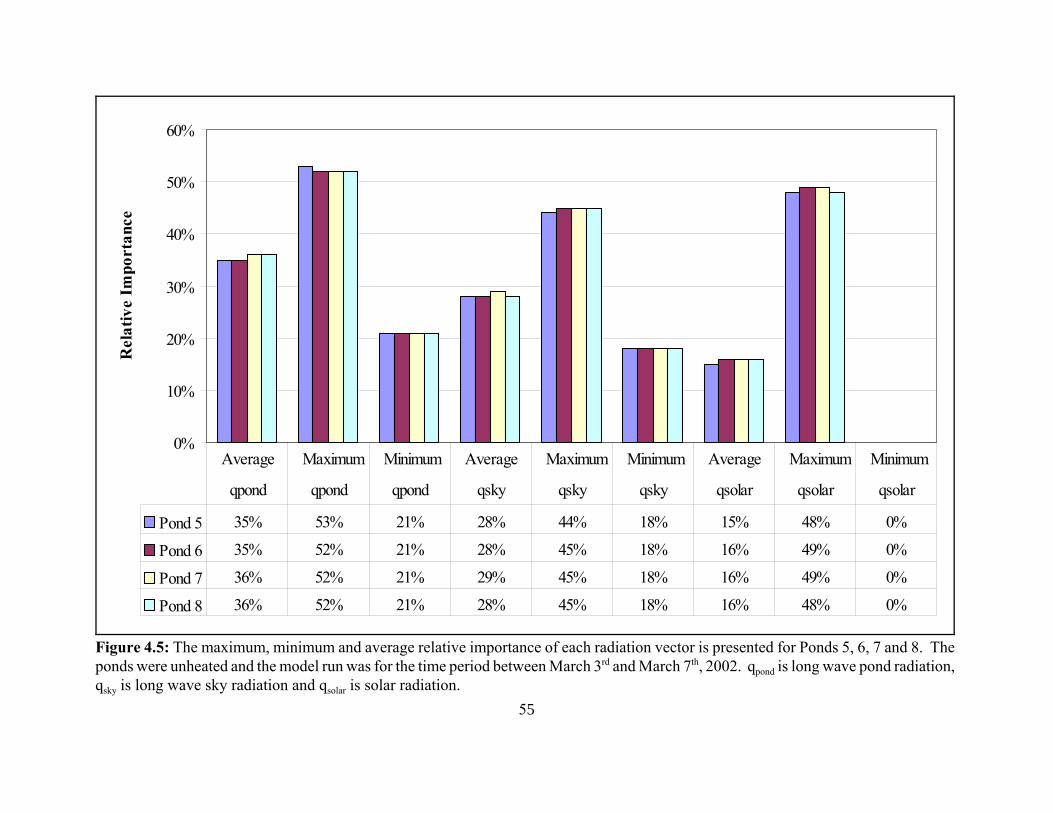
55

0%

10%

20%

30%

40%

50%

60%R

elat

ive

Impo

rtan

ce

Pond 5 35% 53% 21% 28% 44% 18% 15% 48% 0%

Pond 6 35% 52% 21% 28% 45% 18% 16% 49% 0%

Pond 7 36% 52% 21% 29% 45% 18% 16% 49% 0%

Pond 8 36% 52% 21% 28% 45% 18% 16% 48% 0%

Average Maximum Minimum Average Maximum Minimum Average Maximum Minimum

qpond qpond qpond qsky qsky qsky qsolar qsolar qsolar

Figure 4.5: The maximum, minimum and average relative importance of each radiation vector is presented for Ponds 5, 6, 7 and 8. Theponds were unheated and the model run was for the time period between March 3rd and March 7th, 2002. qpond is long wave pond radiation,qsky is long wave sky radiation and qsolar is solar radiation.

56

0%

10%

20%

30%

40%

50%

60%R

elat

ive

Impo

rtan

ce

Pond 13 (1st run) 42% 54% 21% 34% 47% 16% 9% 48% 0%

Pond 13 (2nd run) 40% 54% 19% 32% 46% 14% 10% 48% 0%

Pond 3 41% 54% 18% 35% 47% 15% 10% 55% 0%

Average Maximum Minimum Average Maximum Minimum Average Maximum Minimum

qpond qpond qpond qsky qsky qsky qsolar qsolar qsolar

Figure 4.6: The maximum, minimum and average relative importance of each radiation vector is presented fro both Pond 13 model runsand Pond 3. The ponds were unheated. The first model run for Pond 13 was between November 9 and December 16, 2002. The secondPond 13 model run was for the time between December 25, 2002 and January 24, 2003. The period for the Pond 3 model run wasbetween February 13 and March 23, 2003. qpond is long wave pond radiation, qsky is long wave sky radiation and qsolar is solar radiation.

57

0%

5%

10%

15%

20%

25%

30%

35%R

elat

ive

Impo

rtan

ce

Pond 5 2% 6% 0% 13% 30% 0% 6% 16% 0%

Pond 6 2% 6% 0% 12% 29% 0% 6% 15% 0%

Pond 7 2% 6% 0% 12% 29% 0% 6% 15% 0%

Pond 8 2% 6% 0% 12% 28% 0% 6% 15% 0%

Average Maximum Minimum Average Maximum Minimum Average Maximum Minimum

qsoil qsoil qsoil qevap qevap qevap qconv qconv qconv

Figure 4.7: The maximum, minimum and average relative importance for soil conduction (qsoil), evaporation (qevap) and surfaceconvection (qconv) are presented for Ponds 5, 6, 7 and 8. The ponds were unheated and the model run was for the time period betweenApril 3 and April 7, 2002.

58

0%

5%

10%

15%

20%

25%

30%R

elat

ive

Impo

rtanc

e

Pond 13 (1st run) 6% 13% 0% 4% 26% 0% 4% 21% 0%

Pond 13 (2nd run) 6% 13% 0% 6% 27% 0% 5% 24% 0%

Pond 3 6% 12% 0% 4% 28% 0% 4% 21% 0%

Average Maximum Minimum Average Maximum Minimum Average Maximum Minimum

qsoil qsoil qsoil qevap qevap qevap qconv qconv qconv

Figure 4.8: The maximum, minimum and average relative importance of soil conduction (qsoil), evaporation (qevap and surface convection(qconv) are presented for both Pond 13 model runs and Pond 3. The ponds were unheated. The first model run for Pond 13 was betweenNomber 9 and December 16, 2002. The second Pond 13 model run was for the time between December 25, 2002 and January 24, 2003.The period for the Pond 3 model run was between February 13 and March 23, 2003.

59

1517192123252729313335

2/13 2/19 2/25 3/3 3/9 3/15 3/21

Date

Tem

pera

ture

(°C

)Modeled Pond Temperature

Measured Pond Temperature

Figure 4.9: The modeled and measured temperatures for Pond 12 were plotted againsttime. The model had a tendency of over-predicting the pond temperature (average biasof 2.6°C) but the shape of the curves is similar (correlation coefficient = 0.92).

10

15

20

25

30

35

10 15 20 25 30 35

M easured Pond Temperature (°C)

Mod

eled

Tem

pera

ture

(°C

)

Figure 4.10: For Pond 12, from 02/13 to 03/22, 2003, the correlation coefficient was0.92.

60

0%

20%

40%

60%R

elat

ive

Impo

rtanc

e

Pond Radiation 25% 50% 3%

Sky Radiation 19% 43% 2%

Solar Radiation 7% 50% 0%

Average Max Min

0%

10%

20%

30%

40%

50%

Rel

ativ

e Im

porta

nce

Soil Conduction 1% 6% 0%

Air Coinvection 6% 27% 0%

Evaporation 10% 41% 0%

Average Max Min

0%

20%

40%

60%

80%

Rel

ativ

e Im

porta

nce

Inflow 19% 60% 0%

Outflow 15% 44% 0%

Average Max Min

Figure 4.11: The relative importance of each vector for heated Ponds 9 and 12 arepresented. The model runs were for February 13 to March 22, 2003.

61

-3.00-2.00-1.000.001.002.003.004.005.006.007.00

Average bias 1.55 1.60 1.62 1.62 1.63 1.51 6.16 -2.12

Standard deviation 1.07 1.06 1.09 1.17 1.30 1.46 3.17 1.36

10 min 30 min 1 hr 2 hrs 4 hrs 6 hrs 12 hrs 24 hrs

Figure 4.12: Stability analysis for an unheated pond (Pond 13, between November 13 and Decmber 16, 2002) was done for the showntime steps. The average bias and the standard deviation are in degrees Celcius.

62

0.60

0.65

0.70

0.75

0.80

0.85

0.90

0.95

1.00

10 min 30 min 1 hr 2 hrs 4 hrs 6 hrs 12 hrs

Figure 4.13: Correlation coefficients for the stability analysis for an unheated pond (Pond 13, between November 13 and December 16,2002) were done for the shown time steps. Correlation coefficients were done between the measured and modeled pond temperature runs.

63

0.000.100.200.300.400.500.600.700.800.90

10minutes

30minutes

1 hour 2 hours 4 hours 6 hours 12 hours 24 hours

Figure 4.15: These are the correlation coefficients for the model runs in the stability analysisfor heated ponds. (Pond 12, between the February 13 and March 23).

-3.0-2.0-1.00.01.02.03.04.05.06.07.0

Average Bias 2.7 2.8 2.6 2.5 2.4 2.4 2.3 -2.2

Standard Deviation 1.1 1.2 1.6 1.7 2.6 2.7 4.0 6.0

10 minutes

30 minutes

1 hour 2 hours 4 hours 6 hours 12 hours

24 hours

Figure 4.14: These are the results from the stability analysis for a heated Pond 12between February 13 and March 23, 2003. The average bias and the standarddeviation are in degrees Celsius.

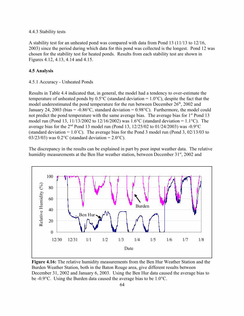
64

0

20

40

60

80

100

12/30 12/31 1/1 1/2 1/3 1/4 1/5 1/6 1/7 1/8

Date

Rel

ativ

e H

umid

ity (%

)

Ben Hur

Burden

Figure 4.16: The relative humidity measurements from the Ben Hur Weather Station and theBurden Weather Station, both in the Baton Rouge area, give different results betweenDecember 31, 2002 and January 6, 2003. Using the Ben Hur data caused the average bias tobe -0.9°C. Using the Burden data caused the average bias to be 1.0°C.

4.4.3 Stability tests

A stability test for an unheated pond was compared with data from Pond 13 (11/13 to 12/16,2003) since the period during which data for this pond was collected is the longest. Pond 12 waschosen for the stability test for heated ponds. Results from each stability test are shown inFigures 4.12, 4.13, 4.14 and 4.15.

4.5 Analysis

4.5.1 Accuracy - Unheated Ponds

Results in Table 4.4 indicated that, in general, the model had a tendency to over-estimate thetemperature of unheated ponds by 0.5°C (standard deviation = 1.0°C), despite the fact that themodel underestimated the pond temperature for the run between December 26th, 2002 andJanuary 24, 2003 (bias = -0.86°C, standard deviation = 0.98°C). Furthermore, the model couldnot predict the pond temperature with the same average bias. The average bias for 1st Pond 13model run (Pond 13, 11/13/2002 to 12/16/2002) was 1.6°C (standard deviation = 1.1°C). Theaverage bias for the 2nd Pond 13 model run (Pond 13, 12/25/02 to 01/24/2003) was -0.9°C(standard deviation = 1.0/C). The average bias for the Pond 3 model run (Pond 3, 02/13/03 to03/23/03) was 0.2°C (standard deviation = 2.0°C).

The discrepancy in the results can be explained in part by poor input weather data. The relativehumidity measurements at the Ben Hur weather station, between December 31st, 2002 and

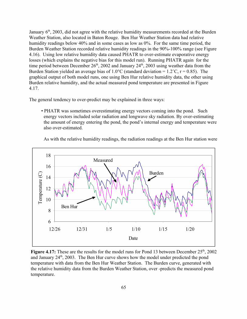
65

6

8

10

12

14

16

18

12/26 12/31 1/5 1/10 1/15 1/20

Date

Tem

pera

ture

(C)

Measured

Ben Hur

Burden

Figure 4.17: These are the results for the model runs for Pond 13 between December 25th, 2002and January 24th, 2003. The Ben Hur curve shows how the model under predicted the pondtemperature with data from the Ben Hur Weather Station. The Burden curve, generated withthe relative humidity data from the Burden Weather Station, over -predicts the measured pondtemperature.

January 6th, 2003, did not agree with the relative humidity measurements recorded at the BurdenWeather Station, also located in Baton Rouge. Ben Hur Weather Station data had relativehumidity readings below 40% and in some cases as low as 0%. For the same time period, theBurden Weather Station recorded relative humidity readings in the 90%-100% range (see Figure4.16). Using low relative humidity data caused PHATR to over-estimate evaporative energylosses (which explains the negative bias for this model run). Running PHATR again for thetime period between December 26th, 2002 and January 24th, 2003 using weather data from theBurden Station yielded an average bias of 1.0°C (standard deviation = 1.2/C, r = 0.85). Thegraphical output of both model runs, one using Ben Hur relative humidity data, the other usingBurden relative humidity, and the actual measured pond temperature are presented in Figure4.17.

The general tendency to over-predict may be explained in three ways:

• PHATR was sometimes overestimating energy vectors coming into the pond. Suchenergy vectors included solar radiation and longwave sky radiation. By over-estimatingthe amount of energy entering the pond, the pond’s internal energy and temperature werealso over-estimated.

As with the relative humidity readings, the radiation readings at the Ben Hur station were

66

suspect. Radiation readings at the Burden Station were lower than those at Ben Hur. Forinstance, for the month of January, 2003, Ben Hur Station radiation measurements were20W greater than Burden Station radiation measurements (standard deviation = 53W).Running PHATR for the first Pond 13 model run (11/09/02 to 12/16/02) using BurdenStation weather data yielded an average bias of 1.6°C (standard deviation =1.06°C) asopposed to an average bias of 1.6°C obtained for Ben Hur weather data. For the secondPond 13 model run (12/26/02 to 01/24/03), the average bias was 0.1°C (standarddeviation 1.1°C) as opposed to an average bias of 1.0°C using Ben Hur weather data. These results suggest that input data did have an effect on how well PHATR predictedpond temperature.

The equation used by PHATR to estimate longwave sky radiation assumes that the sky iscloudless and the atmosphere can be considered as stratified layers of different gasmixtures. If this was not the case (because of turbulence from a weather front), then theunderlying assumptions used by Bliss (1961) to develop Equation 3.26 (the equation usedto determine the sky’s emissivity) were no longer valid. For the present case, Equation3.26 was not necessarily accurate. A pyrgeometer would have to be used to directlymeasure long wave sky radiation.

• PHATR was underestimating energy losses, probably because the evaporation rate wasbeing underestimated. Evaporation, on average, accounted for 12% of all energy intransit for the spring model runs and 5% of all energy in transit in the fall. However,evaporation’s importance was as high as 30% (see Figure 4.7). Equation 3.71, the LakeHefner Equation, was designed to predict the daily evaporation over a lake using thedaily average wind speed (actually, the units for wind speed used in the original referenceby Anonymous, 1952, are miles per day). This same equation might not have been asaccurate when predicting instantaneous or hourly evaporation rates.

For natural systems, the importance of air convection and soil conduction was between 2and 6% (see Figures 4.7 and 4.8). Because the temperature gradient between the pondand its environment, the driving force behind both heat transfer mechanisms, was small,these vectors were not as important as radiation energy transfer mechanisms (forinstance, the average importance for long wave sky radiation ranged from 28% to 35%;see Figures 4.5 and 4.6). Therefore, even if both these vectors were not properlyestimated, the weight of their errors was small and should not be used to explainPHATR’s tendency to over-predict pond temperature.

• PHATR might not have been taking into account other energy transfer mechanisms. Such mechanisms could have been scattered solar radiation which was reflected out ofthe pond. Light, usually greenish light, was poorly absorbed by phytoplankton andwater. Green light (average wavelength at 550 nm, Smith and Cooper, 1957) represented12% of the total solar radiation (see Table 3.2) or 6% of all energy fluxes into and out ofthe pond when the importance of solar radiation was at its peak (49% Pond 6 and 7; see

67

12

13

14

15

16

17

18

19

0:00 12:00 0:00 12:00 0:00 12:00

Time

Tem

pera

ture

(°C

)

Measured

Modeled

Plateau

Figure 4.18: In addition to over-predicting the actual pond temperature, the modeled curve has asmaller amplitude and has plateaus. The smaller amplitude could be caused by an under-estimatingthe pond volume. The plateaus were caused by not properly modeling soil conduction. This is partof the first Pond 13 model run, between November 21 and 23, 2003.

(4.9)

Figure 4.5). Assuming that the pond was absorbing all solar radiation, PHATR would over-predict the pond temperature. Running PHATR for Pond 13 between 11/13/02 and 12/16/02 withmodified solar radiation data (88% of the total measured solar radiation data) yielded betterresults (average bias = 0.9°C; standard deviation = 1.0°C).

In addition to the differences in bias, there were other differences between the modeled andmeasured results. For instance, the diurnal fluctuations in the measured data were greater thanthose in the modeled data. This difference, seen in Figure 4.18, was explained with thefollowing two reasons. First, the thermal mass of Pond 13 may have been over-estimated (theremay have been less water in pond than estimated). Mathematically, this makes sense. Assumingthe pond temperature was a sinusoidal function of time (f(t)), the energy in the pond at any giventime was (E = 0 when T = 0/C)

( )E c T kf tp= ∀ =ρ

where E is the pond energyf(t) is a sinusoidal function of timeD is the density of waterœ is the pond volumecp is the specific heat of water

68

(4.10)

5

10

15

20

25

11/8 11/13 11/18 11/23 11/28 12/3 12/8 12/13

Date

Tem

pera

ture

(°C

)

0 cm 2.5 cm 5 cm 7.5 cm 10 cm 15 cm 20 cm

Figure 4.19: These are the measured temperatures curves for Pond 13 between November 9and December 16, 2002. The top most curve is the pond temperature 20 cm below the watersurface. Many of the curves are super-imposed over each other, meaning that the pond waswell mixed. Because of this, the temperature at any depth can be used as a reference tocompare model runs.

T is the pond temperaturek is a constant

Isolating T yielded:

Tkc

f tp

=∀ρ

( )

where (k/Dcpœ) is the amplitude of f(t).

If the pond volume was overestimated, the amplitude of the modeled temperature function (f(t))would be smaller, as was the case in Figure 4.18.

The amplitude of the measured and modeled temperature curves may also have differed becauseof the choice of location to measure the standard pond reference temperature. Although thereference temperature was measured 10 cm from the surface, the temperature in the bulk fluidand at the surface were visibly similar to each other (see Figure 4.19). For this reason, it was notlikely that the location where the reference temperature was measured was the cause for thedifferent amplitudes between the two curves.

The shape of the measured and modeled curves was also different. A small “plateau”, not

69

8

9

10

11

12

13

12/9 12/10 12/11 12/12 12/13 12/14

Date

Tem

pera

ture

(°C

)

-40000

-30000

-20000-10000

0

10000

2000030000

40000

50000

Rate of H

eat Transfer (W)

Modeled

Measured

Conduction

Figure 4.20: The sinusoid curve is the modeled conduction curve. As conduction begins todecrease, the modeled curve drops. There are no plateaus in the measured pond curve, whichmeans the conduction curve is out of phase.

present in the measured curve, was present in the modeled curve each time the temperaturedecreased (see Figures 18 and 20). Closer examination revealed that these changes in slopeoccurred each night at the same time. This change in slope was caused by not properly modelingsoil conduction. The daily phase angle (see Equation 3.41) which shifted the conduction curvein Figure 20 caused the pond temperature to decrease just as the heat transfer due to soilconduction reaches its peak. Without taking into account the effects of soil heat transfer, theaverage bias for Pond 13 between 11/09/02 and 12/16/02 was 1.37 °C (standard deviation =1.0°C ; r = 0.96). Therefore, using a phase angle of B/2 was not proper. Because there was nochange in slope for the measured curve while the temperature dropped (i.e. there did not seem tobe a lag between the soil surface maximum temperature and the pond maximum temperature),the daily phase angle should be based on the time when the daily pond temperature maximumoccurred. The maximum pond temperature normally occurred between 14:00 and 17:00. Assuming that the maximum occurs at 16:00, the daily phase angle is -5B/6 (see Appendix 5).

Energy transfer mechanisms which were important to uncontrolled ponds were dominated byradiation heat transfer mechanisms. Figures 4.5 and 4.6 reveal that the average importance ofpond radiation, longwave sky radiation and solar radiation ranged between 15 and 54%,depending on the time of day and year. Solar and longwave sky radiation were therefore the twomost important influxes of energy for unheated ponds while pond radiation was the greatestsource of heat loss. Evaporation also seemed to be important (range: 0 to 30%) although its

70

average importance was small (4% to 13%) compared to the radiation heat transfer mechanisms. Air convection (average importance = 4% to 6%) and soil conduction (average importance = 2%to 6%) were not as important because the temperature difference which drove these heat transfermechanisms was relatively small.

4.5.2 Accuracy - Heated Ponds

The average bias for heated pond model runs was 2.4°C (standard deviation = 1.25°C), higherthan the average bias for unheated pond model runs 0.5°C (standard deviation = 0.99°C). Inparticular, the average bias for the Pond 3 model run, a model run for the same time period as theheated pond model runs, was 0.2 °C (standard deviation = 2.0°C). There are four possiblereasons for this:

1) The importance of surface convection and evaporation was greater for heated ponds because of the greater temperature gradient between the pond and the air. Both sets ofequations used by PHATR to predict the size of both surface energy vectors wereempirical and might not have been accurate when they dominated other modes of energytransfer. This happened at night or on cloudy days when there was little solar radiationand no bulk movements of energy associated with water flows. For instance, on the 22nd

of February, 2003, the average importance of evaporation between 11:00 and 16:00 was26% while the average importance of solar radiation was 16% (a cloudy day). Duringthis period of time, the measured temperature declined at a faster rate than the modeledtemperature, causing the bias to increase from 0.3°C to 1.5°C (see Figure 4.21). Thismight have been caused by the evaporation being under-estimated by the model.

2) The flow of water into and out of the pond varied from the estimated flows used by PHATR. The method used to measure the flow rate of warm water assumed that for agiven combination of open and closed valves along the water line, a fixed flowrate wouldresult. However, this was apparently not the case. For the evening of February 22nd,2003, the well was turned on at 17:00 and according to the recorded data, all four valveswere open. Normally, water would flow to all four controlled ponds, including pond 12. However, the rate of decline for the measured temperature curve at 17:00 did not change. Rather, the pond only began to warm at 20:00, when one of the valves at another pondclosed. The bias, by this time, had increased from 1.5 to 3.8°C. Apparently, no waterflowed into pond 12, despite the open valve.

3) The method used to measure the flowrate might have had a large measurement error.The flow rate was measured by timing the period it took to fill a 120-liter bucket with100 liters of water. The measurement has an accuracy of ±1 second. When only onevalve was open, measuring the flow rate took 5 seconds. This translated into a possiblerelative error of 17 to 24% when estimating the bulk energy flow rate (see Table 4.6).

71

20

22

24

26

28

30

0:00 12:00 0:00 12:00 0:00

Time

Tem

pera

ture

(°C

)

0

200000

400000

600000

800000

1000000

1200000

1400000B

ulk energy flow rates (W

) Measured

Modeled

Flow

Figure 4.21: This data represents the pond temperature and warm water flow for Pond 12 onFebruary 22 and February 23, 2003. During the first afternoon, the measured pondtemperature decreased faster than the modeled pond temperature, revealing that evaporationmight be underestimated. At 17:00 on the first afternoon, warm water supposedly flowedinto the pond. However, the pond temperature only began to rise at 20:00, when a valve onanother pond closed. This means that water only began to flow into Pond 12 at 20:00, not at17:00. As can be seen, PHATR’s accuracy is dependant on the quality of the collected dataand the validity of its equations.

Table 4.6: If 5 seconds were measured to fill a 120 liter bucket when it really took 4, PHATR under-estimated the energy flow rate by 25% . If it really took 6 seconds to fill the bucket, the model over-predicted the bulk energy flow rate by 17%.

Time (s)

Flow rate (m3/s)

Bulk Energy Flowrate(W)

RelativeError

4 0.026 988693 25%

5 0.021 790954 ---

6 0.018 659128 17%

The implications of such errors in measurements can be grasped through a numericalexample. Consider Pond 12 (volume = 342 m3) at night (no solar radiation) with warm

72

(4.11)

(4.12)

effluent water flowing in at 36°C and flowing out at 27°C. Water losses due toevaporation were negligible so the flow rates into and out of the pond were the same. Energy losses due to surface evaporation, air convection and soil conduction were small(on average, these energy vectors together represented no more than 17% of the totalenergy flux in the absence of bulk fluid, and represented much less when there was warmwater entering the pond). Pond radiation and sky radiation were balanced. Byperforming an energy balance for this example, Equation 3.4 reduces to:

dEdt

q qwell out= −

or

( )ρ ρcdTdt

c T Tp pond p flow well∀ = ∀ −&

where E is the internal energy of the pond,D is the density of water, cp is the specific heat of water, œpond is the volume of the pond, T is the temperature of the pond, t is time,

is the flow rate of warm water into the pond &∀ flow

Twell is the temperature of the warm water (36°C).

For a flow rate of 0.018 m3/s, the rate at which the pond heats up (dT/dt) is 1.7°C/hr. Fora flow rate of 0.026 m3/s, the rate at which the pond heats up is 2.5°C/hr, a difference(bias) of 0.8°C/hr. Consequently, errors in flow measurements can have an effect on themodel’s bias, especially if there is more water flowing than estimated.

4) The time step was too large. Unlike other energy transfer mechanisms, the flow ofwarm water was a discrete-event energy transfer vector (i.e. bulk energy flow rateschanged within seconds). Because of this, modeling with large time steps was notappropriate. For example, if a valve were to open 50 minutes before the X:00, andPHATR was using data sampled every hour (X:00), PHATR would have ignored theeffects of heating the pond 50 minutes prior to that hour reading. Similarly, if a valvewere to close one minute after the hour, PHATR would wrongly have assumed that thevalve was open for the next 59 minutes. This affected the bias (which can increase ordecrease, depending on the situation) but more importantly, this affected the model’sability to predict change (reflected in the correlation coefficient). The correlationcoefficient decreased from 0.92 (step size = 1 hour) to 0.83 (step size = 4 hours) to 0.70(step size = 6 hours).

73

Because the movement of water was an important energy vector(as important as 60%), mosterrors in the model’s output were caused by poorly estimating flow. To fully understand theimportance of bulk water movements to the energy balance, consider and compare the size ofthese energy vectors with solar radiation. On a clear sunny day in summer, solar power may beas high as 1000 W/m2. For Pond 12, with an area of 280 m2, this represented a heat transfer rateof 280 kW. To produce the same net energy flux with bulk flow, the flow rate must be 451 litersper minute (119 gpm), assuming the well water is 36°C and the discharged water is 27°C. Thisflow rate is moderately high. So for the purposes of comparison, warm water flow can beconsidered as a night time substitute for sunlight. Flow is as important an energy transfermechanism as sunlight and by failing to properly estimate flow, PHATR’s accuracy suffers.

4.5.3 Stability Analysis - Unheated Ponds

The average bias for a model run using a step size of 6 hours was 1.5°C while the average biasfor a model run using a step size of 10 minutes was also 1.5°C (see Figure 4.12). For a 12 hourstep size, the average bias was 6.2 °C. Only when using a step size of 24 hours was the averagebias negative (-2.1°C). This was because the solar radiation in the input weather data, sampledat midnight, was always 0 W/m2. The model’s ability to predict change was reflected in thecorrelation coefficients, ranging from 0.96 for a step size of 10 minutes to 0.92 for a step size of6 hours (see Figure 4.13). Only for a step size of 12 hours was the correlation coefficient below0.90 (0.62).

In spite of the presented data, using a step size of 6 hours to run PHATR was not recommended. By using a step size of 6 hours, the output lost detail. The average bias between two model runs,step sizes = 6 hours and 1 hour, is 0.7°C (standard deviation = 0.6°C). The average bias betweentwo model runs, step size = 10 minutes and 1 hour, was 0.1°C (standard deviation = 0.1°C). Therefore, a step size of 1 hour should have been suitable in maintaining a fair amount of detailin the output.

4.5.4 Stability Analysis - Heated Ponds

Increasing the step size had no effect on decreasing the average bias. The average bias for amodel run with a 10 minute step size was 2.7°C while a model run with a step size of 6 hourshad a bias of 2.4°C (see Figure 4.14). However, the standard deviation never exceeded 1.2°C forstep sizes 30 minutes or less. Smaller step sizes minimized the error associated withmiscalculating the flow of warm water and energy entering a pond. PHATR’s ability to predictchange improved by using smaller step sizes (r4 hour = 0.83, r10 min= 0.95; see Figure 4.15). Therefore, because of the discrete nature of bulk energy fluxes, the model’s ability to predicttemperature changes in heated ponds depended on a small step size. For heated ponds, a stepsize of 10 or 30 minutes was appropriate.

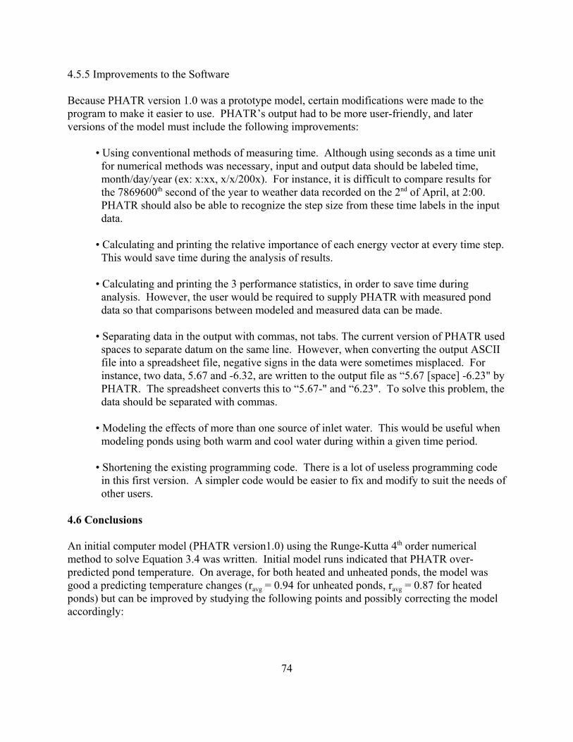
74

4.5.5 Improvements to the Software

Because PHATR version 1.0 was a prototype model, certain modifications were made to theprogram to make it easier to use. PHATR’s output had to be more user-friendly, and laterversions of the model must include the following improvements:

• Using conventional methods of measuring time. Although using seconds as a time unitfor numerical methods was necessary, input and output data should be labeled time,month/day/year (ex: x:xx, x/x/200x). For instance, it is difficult to compare results forthe 7869600th second of the year to weather data recorded on the 2nd of April, at 2:00. PHATR should also be able to recognize the step size from these time labels in the inputdata.

• Calculating and printing the relative importance of each energy vector at every time step. This would save time during the analysis of results.

• Calculating and printing the 3 performance statistics, in order to save time duringanalysis. However, the user would be required to supply PHATR with measured ponddata so that comparisons between modeled and measured data can be made.

• Separating data in the output with commas, not tabs. The current version of PHATR usedspaces to separate datum on the same line. However, when converting the output ASCIIfile into a spreadsheet file, negative signs in the data were sometimes misplaced. Forinstance, two data, 5.67 and -6.32, are written to the output file as “5.67 [space] -6.23" byPHATR. The spreadsheet converts this to “5.67-" and “6.23". To solve this problem, thedata should be separated with commas.

• Modeling the effects of more than one source of inlet water. This would be useful whenmodeling ponds using both warm and cool water during within a given time period.

• Shortening the existing programming code. There is a lot of useless programming codein this first version. A simpler code would be easier to fix and modify to suit the needs ofother users.

4.6 Conclusions

An initial computer model (PHATR version1.0) using the Runge-Kutta 4th order numericalmethod to solve Equation 3.4 was written. Initial model runs indicated that PHATR over-predicted pond temperature. On average, for both heated and unheated ponds, the model wasgood a predicting temperature changes (ravg = 0.94 for unheated ponds, ravg = 0.87 for heatedponds) but can be improved by studying the following points and possibly correcting the modelaccordingly:

75

Pond

Back Radiation 35-42%

Longwave sky Radiation 28-35%

Cloud

Soil 2-6%

Evaporation 4-13%

Convection 4-6%

Solar Radiation

9-16%

Pond

Back Radiation 35-42%

Longwave sky Radiation 28-35%

Cloud

Soil 2-6%

Evaporation 4-13%

Convection 4-6%

Solar Radiation

9-16%

Figure 4.22: An energy balance for unheated ponds was performed during the fall of 2002 andspring 2002 - 2003 in Baton Rouge, Louisiana. The average relative importance of each energyvector is shown. For unheated ponds, longwave radiation mechanisms were more important.The importance of solar radiation during the day was found to be as high as 55%.

• the effects of light being reflected at the pond surface (when the sun is low in the sky)and the extinction of light in the pond water

• the true rate of evaporation and surface convection for this particular set of ponds • the thermal properties of the pond soil

Major vectors of energy transfer for unheated ponds were found to be radiation heat transfermechanisms (Figure 4.22). For heated ponds, bulk energy flow rates were also important. Surface convection and evaporation were important when there was no solar radiation or waterflowing into the pond (Figure 4.23). The modeled heat conducted through the soil had anegative effect on PHATR’s ability to predict change. An appropriate step size for unheatedpond model runs was found to be 1 hour. An appropriate step size for heated pond model runswas found to be 10 to 30 minutes.

Improvements to the software were recommended to simplify analysis of the output data.

76

Influent 19%

PondEffluent

15%

Back Radiation 25%

Longwave sky Radiation 19%

Cloud

Soil 1%

Evaporation 10%

Convection 6%

Solar Radiation 7%

Influent 19%

PondEffluent

15%

Back Radiation 25%

Longwave sky Radiation 19%

Cloud

Soil 1%

Evaporation 10%

Convection 6%

Solar Radiation 7%

Figure 4.23: an energy balance for heated ponds was performed during the spring of 2003 inBaton Rouge, Louisiana. The average relative importance for each energy vector is shown. Inaddition to longwave radiation, water entering and leaving the pond represented importantenergy vectors. The importance of warm influent was as high as 60%. The importance of theeffluent was as high as 44%. Solar radiation accounted for as much as 50% of all energymovements.

77

(5.1)

CHAPTER 5: THE EXPERIMENTAL DETERMINATION OF PARAMETERSIMPORTANT TO HEAT TRANSFER IN PONDS

5.1 Introduction

A computer model, PHATR (Pond Heating And Temperature Regulation), used to model energybalances for aquaculture ponds was developed in Chapter 4. Based on the findings from theprevious chapter, parameters that could improve PHATR’s accuracy were determinedexperimentally. These parameters were:

• the convection mass transfer (evaporation) coefficient, hm• the convection heat transfer coefficient at the pond surface, h• the extinction coefficient of the pond, $• the albedo of the pond

Because heat conducted through the soil was less important compared to other energy transfermechanisms, soil thermal properties were not determined. Each of these parameters weredetermined either through field experiments or by analysis of existing data.

5.2 Theory

5.2.1 The Heat and Mass Transfer Coefficients

Two approaches were used to determine the heat and mass transfer coefficients. The firstconsisted of using the heat and mass transfer analogy (Incropera and De Witt, 1985) to findanalytical values for the coefficients. The second consisted in comparing empirical equationsfound in the literature used to predict the evaporation and convection rates.

• Heat and mass transfer analogy: the heat and mass transfer analogy relies on themathematical and physical similarities of heat and mass transfer at the pond surface. Bothtransport phenomena are controlled by the velocity (wind) boundary layer and both aregoverned by the same mathematical equation (the diffusion equation) with the same typeof boundary conditions. Convection coefficients used in heat and mass transfer aredetermined using analogous empirical equations and, as is demonstrated in Appendix 6,can be related to one another with Equation 5.1:

h h c Lem air p air= −ρ2

3

where h is the convective heat transfer coefficient, hm is the convective mass transfer coefficient, Dair is the density of dry air, cp-air is the specific heat of air at a given moisture content and Le is the Lewis number, a dimensionless ratio comparing thethermal diffusivity to the mass diffusivity.

78

(5.2)

Scattered light

Shadow

Scattered light

Pyranometer

Solar RadiationAir

Water

Scattered light

Shadow

Scattered light

Pyranometer

Solar RadiationAir

Water

Figure 5.1: Measuring scattered radiationleaving the pond is difficult because of theshadow cast by the pyranometer (facingdown in the diagram). Normally, solarradiation would contribute to the scattering.However, because the pyranometer blockingsolar radiation, the solar radiation’scontribution cannot be measured.

•Comparison of empirical equations in the literature: The three empirical equations in theliterature review used to predict evaporation (Chapter 3.5.2) were Equation 3.67(Penman, 1948), Equation 3.70 (Piedrahita, 1991) and Equation 3.71 (Anonymous,1952). The two empirical equations in the literature review used to predict heatconvection (Chapter 3.4) were Equation 3.58 (Watmuff et al., 1977) and Equations 3.49through 3.57 (Nusselt Number correlations; Holman, 1997). PHATR Version 1.0 usedEquation 3.71 (the Lake Hefner Equation) to predict the rate of evaporation and Equation3.58 to estimate the convection coefficient.

5.2.2 Extinction Coefficient

The extinction coefficient is the parameter that quantifies extinction of light in a medium (seeChapters 3.2.2.2 and 3.2.2.3). It can be estimated by manipulating the Bouger-Beer Law. Solving Equation 3.10 yields:

ln lnq q zsolar= − β

where q is the radiation (W) at depth z (m or mm), qsolar is the solar radiation (W) and$ is the extinction coefficient (m-1 or mm-1).

By plotting the natural logarithm of solar radiation(ln qsolar) versus the depth (z), the extinctioncoefficient can be determined by calculating theslope of the line of best fit.

5.2.3 Albedo

Table 3.3, based on Fresnel and Snell’s Laws,shows that only a small percentage of solarradiation is reflected for angles of incidence greaterthan 60°(i.e. for angles of solar elevation less than30° above the horizon). However, more solarradiation could be reflected back to the sky becauseof the effects of scattering. If most suspendedparticles are assumed to be free clay particlesoriginally from the pond bottom, and if the size of aclay particles is defined as smaller than 2 :m indiameter, then, because visible solar radiation(poorly absorbed by pure water) have a wavelengthof between 0.4 and 0.7 :m, a combination ofRayleigh scattering and “macro-scattering”(together known as Mie scattering) occur (Seigel,

79

(5.3)

1981). Mie scattering is difficult to predict and as a result, theoretical calculations can beinaccurate.

Measuring the back scattering of radiation is hampered by the shadow cast by a pyranometer(Figure 5.1). A pyranometer facing down and measuring the light traveling upwards will blockthe incident solar radiation traveling downward. A portion of the solar radiation would normallybe reflected where the pyranometer is located. Unfortunately, this cannot happen because thepyranometer is blocking the path of solar radiation. Therefore, to estimate the albedo, it wasnecessary to calculate this value with an indirect method.

5.3 Materials and Methods

5.3.1 The Heat and Mass Transfer Coefficients - Heat and Mass Transfer Analogy

A modified version of PHATR (Version 1.1) was used to generate heat and mass transfercoefficients by solving for hm, the evaporation mass transfer coefficient, in Equation 3.4:

( )

( )h

dEdt

q q q q q q q q

A Le c T T h MMR

PT

PT

mpond

solar back sky soil seep rain well out

air p air air pond fgsurface air

=

− − + ± − + + −

− −

−

−

2 3/ ρ

Subsequently, Equation 5.1 was used to determine h, the convective heat transfer coefficient. The derivation of Equation 5.3 is provided in Appendix 7. Model runs for PHATR version 1.1were based on input data collected at Pond 13 between November 9th and December 16th, 2002.Weather data, pond temperature data and flow rate data collected at night were used. Unlikeversion 1.0, Version 1.1 used the pond temperature to estimate the rate of internal energy changein the pond. By using data collected only at night in an unheated pond, the solar radiation termand the bulk energy flow rate terms in Equation 5.3 were equal to 0.

Once values for the mass transfer coefficients were generated, a relationship between bothparameters and the wind speed was developed.

5.3.2 The Heat and Mass Transfer Coefficients - Comparison of Empirical Equations

An other modified version of PHATR, Version 1.2, was used to determine if certaincombinations of empirical equations for evaporative and convective energy transfer couldimprove accuracy. Input data consisted of weather and flow rate data collected during Februaryand March, 2003. The model output data was compared to the pond temperature data collectedfor Pond 3 (unheated) and Pond 12 (heated). The three criteria used in Chapter 4 (average biasbetween modeled and measured data, the standard deviation of the average bias and thecorrelation coefficient (r) between the modeled and measured data) were calculated again. Table

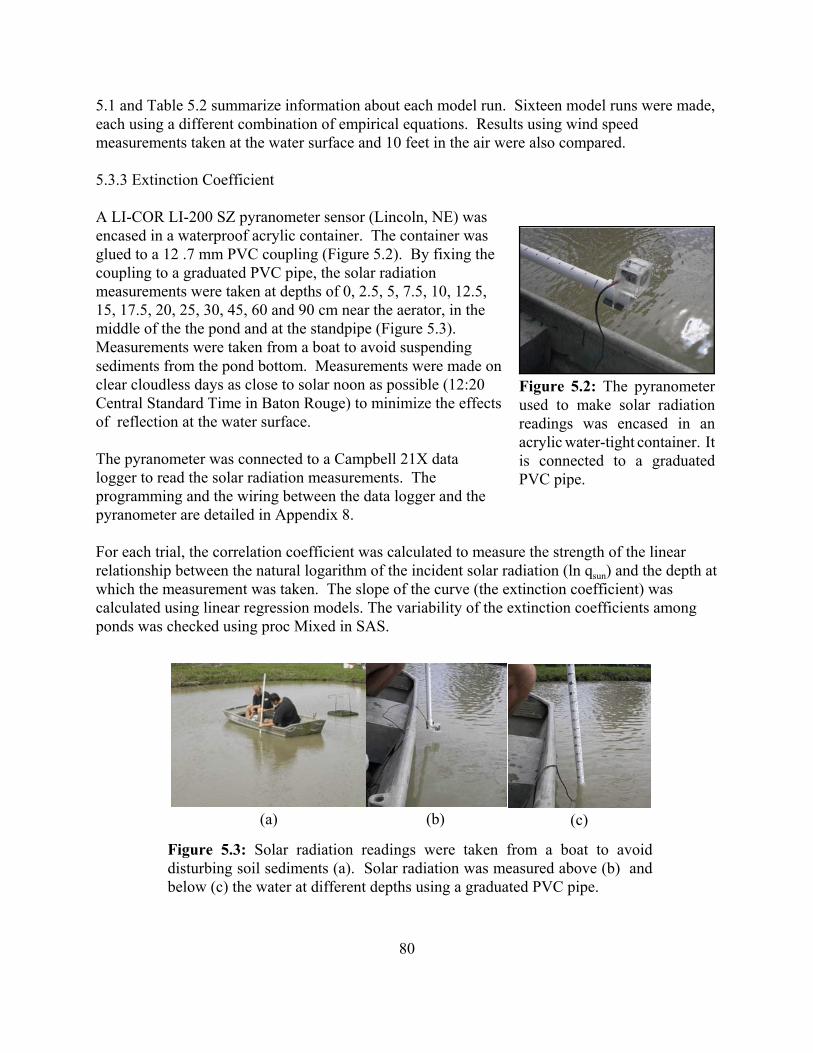
80

Figure 5.2: The pyranometerused to make solar radiationreadings was encased in anacrylic water-tight container. Itis connected to a graduatedPVC pipe.

(a) (b) (c)

5.1 and Table 5.2 summarize information about each model run. Sixteen model runs were made,each using a different combination of empirical equations. Results using wind speedmeasurements taken at the water surface and 10 feet in the air were also compared.

5.3.3 Extinction Coefficient

A LI-COR LI-200 SZ pyranometer sensor (Lincoln, NE) wasencased in a waterproof acrylic container. The container wasglued to a 12 .7 mm PVC coupling (Figure 5.2). By fixing thecoupling to a graduated PVC pipe, the solar radiationmeasurements were taken at depths of 0, 2.5, 5, 7.5, 10, 12.5,15, 17.5, 20, 25, 30, 45, 60 and 90 cm near the aerator, in themiddle of the the pond and at the standpipe (Figure 5.3). Measurements were taken from a boat to avoid suspendingsediments from the pond bottom. Measurements were made onclear cloudless days as close to solar noon as possible (12:20Central Standard Time in Baton Rouge) to minimize the effectsof reflection at the water surface.

The pyranometer was connected to a Campbell 21X datalogger to read the solar radiation measurements. Theprogramming and the wiring between the data logger and thepyranometer are detailed in Appendix 8.

For each trial, the correlation coefficient was calculated to measure the strength of the linearrelationship between the natural logarithm of the incident solar radiation (ln qsun) and the depth atwhich the measurement was taken. The slope of the curve (the extinction coefficient) wascalculated using linear regression models. The variability of the extinction coefficients amongponds was checked using proc Mixed in SAS.

Figure 5.3: Solar radiation readings were taken from a boat to avoiddisturbing soil sediments (a). Solar radiation was measured above (b) andbelow (c) the water at different depths using a graduated PVC pipe.

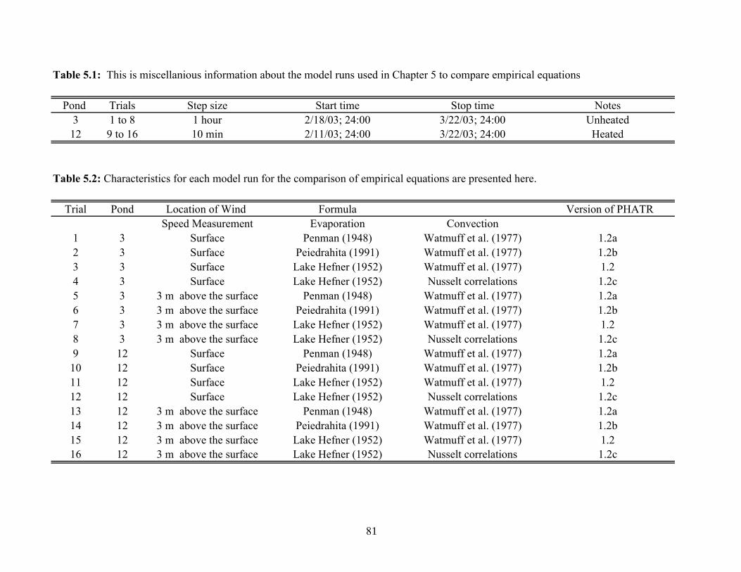
Table 5.1: This is miscellanious information about the model runs used in Chapter 5 to compare empirical equations

Pond Trials Step size Start time Stop time Notes3 1 to 8 1 hour 2/18/03; 24:00 3/22/03; 24:00 Unheated12 9 to 16 10 min 2/11/03; 24:00 3/22/03; 24:00 Heated

Table 5.2: Characteristics for each model run for the comparison of empirical equations are presented here.

Trial Pond Location of Wind Formula Version of PHATR Speed Measurement Evaporation Convection

1 3 Surface Penman (1948) Watmuff et al. (1977) 1.2a2 3 Surface Peiedrahita (1991) Watmuff et al. (1977) 1.2b3 3 Surface Lake Hefner (1952) Watmuff et al. (1977) 1.24 3 Surface Lake Hefner (1952) Nusselt correlations 1.2c5 3 3 m above the surface Penman (1948) Watmuff et al. (1977) 1.2a6 3 3 m above the surface Peiedrahita (1991) Watmuff et al. (1977) 1.2b7 3 3 m above the surface Lake Hefner (1952) Watmuff et al. (1977) 1.28 3 3 m above the surface Lake Hefner (1952) Nusselt correlations 1.2c9 12 Surface Penman (1948) Watmuff et al. (1977) 1.2a10 12 Surface Peiedrahita (1991) Watmuff et al. (1977) 1.2b11 12 Surface Lake Hefner (1952) Watmuff et al. (1977) 1.212 12 Surface Lake Hefner (1952) Nusselt correlations 1.2c13 12 3 m above the surface Penman (1948) Watmuff et al. (1977) 1.2a14 12 3 m above the surface Peiedrahita (1991) Watmuff et al. (1977) 1.2b15 12 3 m above the surface Lake Hefner (1952) Watmuff et al. (1977) 1.216 12 3 m above the surface Lake Hefner (1952) Nusselt correlations 1.2c

81

82

5.3.4 The Albedo

Two modified versions of PHATR (Versions 1.21 and 1.21a) were used to determine the albedoof the pond empirically. These versions prompt the user for albedo values. The modelrecalculates the pond temperature, taking the albedo into account. Albedos of 0%, 5%, 10%,15%, 20% and 25% were incorporated into model runs. The three statistical criteria previouslyused (average bias between modeled and measured data, the standard deviation of the averagebias and the correlation coefficient between the modeled and measured data) were againcalculated here. The time step for model runs for Pond 3 and Pond 13 was 1 hour and for Pond12, 10 minutes.

5.4 Results

5.4.1 Heat and Mass Transfer Coefficients - The Heat and Mass Transfer Analogy

Statistical parameters reflecting the results are shown in Table 5.3 Full model run results arepresented graphically in the form of a scatter plot (wind speed vs heat/mass transfer coefficientin Figures 5.4 and 5.5).

Table 5.3: These are statistical parameters describing the accuracy of results from the heat and masstransfer analogy method. h is the heat transfer coefficient and hm is the convective mass transfercoefficient.

Parameter h hm(W/m2/K) (m/s)

Average 27 0.0107Maximum 15146 0.5959Minimum -12515 -1.5029Standard deviation 597 0.0753Standard deviation x 2 1195 0.1507Correlation Coefficient - r 0.003 0.02934

5.4.2 Heat and Mass Transfer Coefficients - Comparison of Empirical Equations

The statistical parameters used for comparing the output from PHATR Version 1.2 trials arepresented in Table 5.4. An example of the model’s output is graphically presented in Figure 5.6.

5.4.3 Extinction Coefficient

Figure 5.7 is an example plot comparing the natural logarithm of incident solar radiation to thedepth at which the measurement was taken. The slope of the line of best fit represents theextinction coefficient. Values for the correlation coefficient (r) and the slope of the line (theextinction coefficient) are presented in Table 5.5. The average correlation coefficient is -0.96,

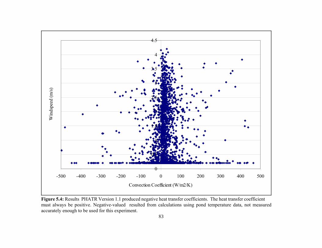
83

0

0.5

1

1.5

2

2.5

3

3.5

4

4.5

-500 -400 -300 -200 -100 0 100 200 300 400 500

Convection Coefficient (W/m2/K)

Win

dspe

ed (m

/s)

Figure 5.4: Results PHATR Version 1.1 produced negative heat transfer coefficients. The heat transfer coefficientmust always be positive. Negative-valued resulted from calculations using pond temperature data, not measuredaccurately enough to be used for this experiment.

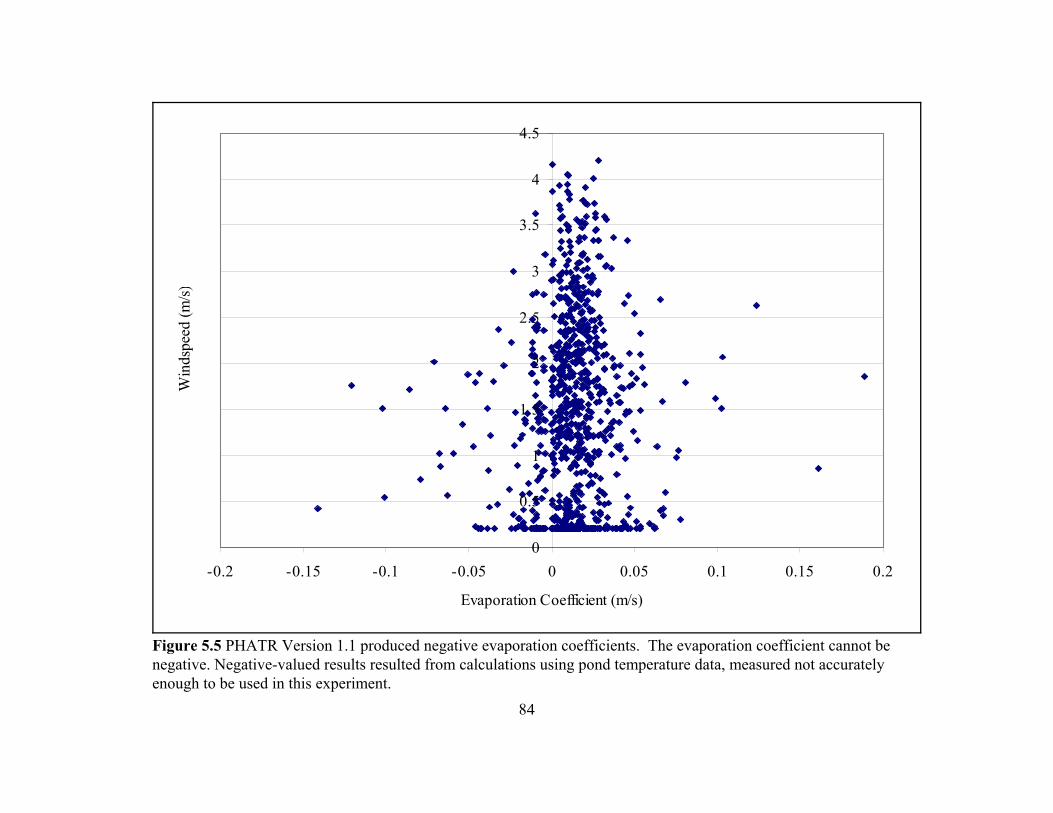
84

0

0.5

1

1.5

2

2.5

3

3.5

4

4.5

-0.2 -0.15 -0.1 -0.05 0 0.05 0.1 0.15 0.2

Evaporation Coefficient (m/s)

Win

dspe

ed (m

/s)

Figure 5.5 PHATR Version 1.1 produced negative evaporation coefficients. The evaporation coefficient cannot benegative. Negative-valued results resulted from calculations using pond temperature data, measured not accuratelyenough to be used in this experiment.

Table 5.4: These are the characteristics and results for each model run for the comparison of empirical evaporation and convection equationThe bias represents the average difference between the model run and the measured data. The standard deviation (St. dev.) and the correlationcoefficient ( r) between the modeled and measured data are presented.

Trial Pond Pond Location of wind Formula StatisticsNumber Treatment speed measurment Evaporation Convection Bias St. Dev. r

1 3 Unheated surface Penman (1948) Watmuff et al. (1997) -4.5 2.2 0.852 3 Unheated surface Piedrahita (1991) Watmuff et al. (1997) -4.4 2.2 0.853 3 Unheated surface Lake Hefner Watmuff et al. (1997) -4.3 2.2 0.864 3 Unheated surface Lake Hefner Nusselt numbers -4.6 2.3 0.855 3 Unheated 3 m above the surface Penman (1948) Watmuff et al. (1997) -0.7 1.8 0.966 3 Unheated 3 m above the surface Piedrahita (1991) Watmuff et al. (1997) 0.5 2.1 0.947 3 Unheated 3 m above the surface Lake Hefner Watmuff et al. (1997) 0.3 2.0 0.948 3 Unheated 3 m above the surface Lake Hefner Nusselt numbers 0.4 2.0 0.939 12 Heated surface Penman (1948) Watmuff et al. (1997) -5.5 2.7 0.6010 12 Heated surface Piedrahita (1991) Watmuff et al. (1997) -5.3 2.8 0.5911 12 Heated surface Lake Hefner Watmuff et al. (1997) -5.1 2.7 0.6012 12 Heated surface Lake Hefner Nusselt numbers -5.1 2.7 0.6113 12 Heated 3 m above the surface Penman (1948) Watmuff et al. (1997) 1.3 0.8 0.9614 12 Heated 3 m above the surface Piedrahita (1991) Watmuff et al. (1997) 3.2 1.1 0.9515 12 Heated 3 m above the surface Lake Hefner Watmuff et al. (1997) 2.9 1.0 0.9516 12 Heated 3 m above the surface Lake Hefner Nusselt numbers 5.0 1.2 0.95

Table 5.4: These are the characteristics and results for each model run for the comparison of empirical evaporation and convectionequations. The bias represents the average difference between the model and the measured data. The standard deviation (St. Dev.) and thecorrelation coefficient ( r) between the modeled and measured data are indicators of the model's ability to predict change (see Chapter 4).

85

86

10

15

20

25

30

35

2/12 2/17 2/22 2/27 3/3 3/8 3/13 3/18

Date

Tem

pera

ture

(°C

)

Measured

(a) (b)

(c)(d)

Figure 5.6: These are the temperature profiles for 4 model runs and the measured pond temperature in a heated Pond 12 between the 13th

of February and the 23rd of March, 2003. The temperature curves were generated using (a) Nusselt Correlations (wind speed measuredat 3 m), (b)Watmuff et al.’s (1977) Equation (wind speed measured at 10 feet), ( c) Nusselt Correlation (wind speed measured at 33 cm)and (d) Watmuff et al’s (1977) Equation (wind speed measured at 33 cm) for estimating convection. (Curves ( c) and (d) aresuperimposed.) Using the wind speed measured at 33 cm caused PHATR to underestimate the pond temperature. This is because theequation used to correct the wind speed cannot be used for wind speeds at low elevations.

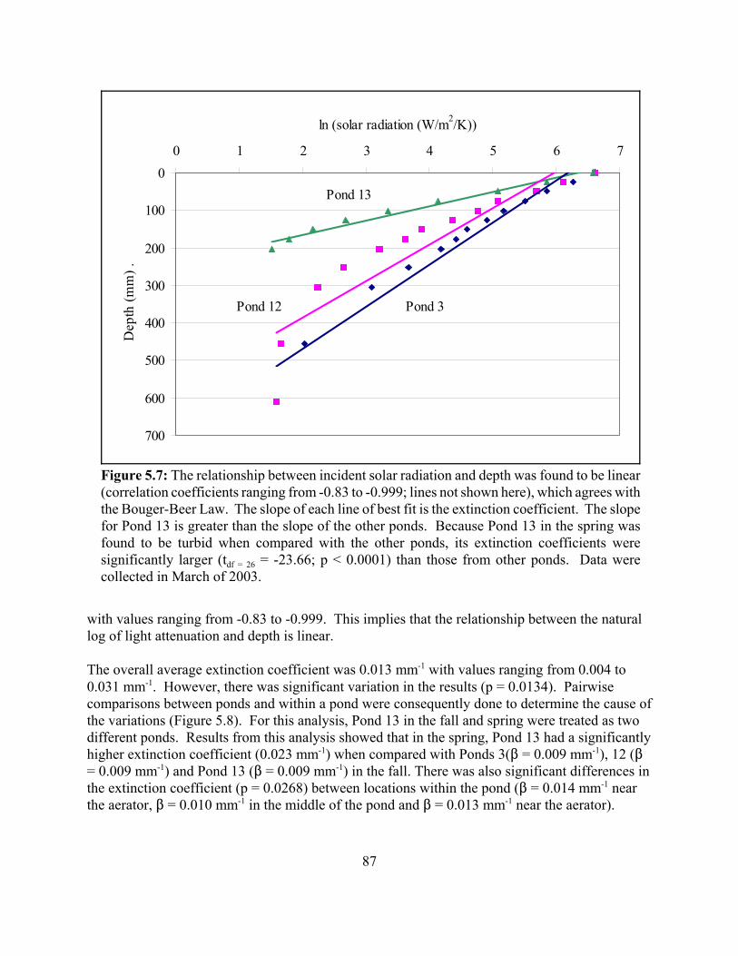
87

0

100

200

300

400

500

600

700

0 1 2 3 4 5 6 7

ln (solar radiation (W/m2/K))D

epth

(mm

) .

Pond 13

Pond 12 Pond 3

Figure 5.7: The relationship between incident solar radiation and depth was found to be linear(correlation coefficients ranging from -0.83 to -0.999; lines not shown here), which agrees withthe Bouger-Beer Law. The slope of each line of best fit is the extinction coefficient. The slopefor Pond 13 is greater than the slope of the other ponds. Because Pond 13 in the spring wasfound to be turbid when compared with the other ponds, its extinction coefficients weresignificantly larger (tdf = 26 = -23.66; p < 0.0001) than those from other ponds. Data werecollected in March of 2003.

with values ranging from -0.83 to -0.999. This implies that the relationship between the naturallog of light attenuation and depth is linear.

The overall average extinction coefficient was 0.013 mm-1 with values ranging from 0.004 to0.031 mm-1. However, there was significant variation in the results (p = 0.0134). Pairwisecomparisons between ponds and within a pond were consequently done to determine the cause ofthe variations (Figure 5.8). For this analysis, Pond 13 in the fall and spring were treated as twodifferent ponds. Results from this analysis showed that in the spring, Pond 13 had a significantlyhigher extinction coefficient (0.023 mm-1) when compared with Ponds 3($ = 0.009 mm-1), 12 ($= 0.009 mm-1) and Pond 13 ($ = 0.009 mm-1) in the fall. There was also significant differences inthe extinction coefficient (p = 0.0268) between locations within the pond ($ = 0.014 mm-1 nearthe aerator, $ = 0.010 mm-1 in the middle of the pond and $ = 0.013 mm-1 near the aerator).

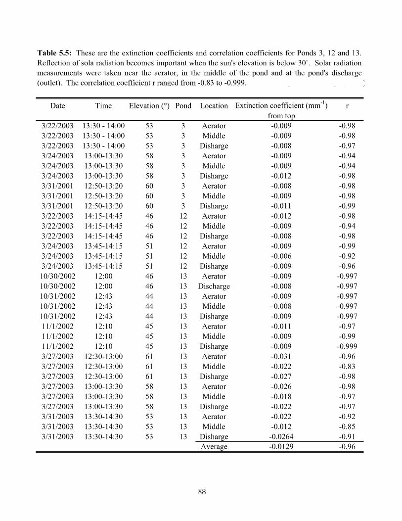
Table 5.5: These are the extinction coefficients and correlation coefficients for Ponds 3, 12 and 13. Reflection of solar radiation becomes important when the sun's elevation is below 30°. Solar radiation measurements were taken near the aerator, in the middle of the pond and at the pond's discharge (outlet)

Date Time Elevation (°) Pond Location Extinction coefficient (mm-1) rfrom top

3/22/2003 13:30 - 14:00 53 3 Aerator -0.009 -0.983/22/2003 13:30 - 14:00 53 3 Middle -0.009 -0.983/22/2003 13:30 - 14:00 53 3 Disharge -0.008 -0.973/24/2003 13:00-13:30 58 3 Aerator -0.009 -0.943/24/2003 13:00-13:30 58 3 Middle -0.009 -0.943/24/2003 13:00-13:30 58 3 Disharge -0.012 -0.983/31/2001 12:50-13:20 60 3 Aerator -0.008 -0.983/31/2001 12:50-13:20 60 3 Middle -0.009 -0.983/31/2001 12:50-13:20 60 3 Disharge -0.011 -0.993/22/2003 14:15-14:45 46 12 Aerator -0.012 -0.983/22/2003 14:15-14:45 46 12 Middle -0.009 -0.943/22/2003 14:15-14:45 46 12 Disharge -0.008 -0.983/24/2003 13:45-14:15 51 12 Aerator -0.009 -0.993/24/2003 13:45-14:15 51 12 Middle -0.006 -0.923/24/2003 13:45-14:15 51 12 Disharge -0.009 -0.9610/30/2002 12:00 46 13 Aerator -0.009 -0.99710/30/2002 12:00 46 13 Discharge -0.008 -0.99710/31/2002 12:43 44 13 Aerator -0.009 -0.99710/31/2002 12:43 44 13 Middle -0.008 -0.99710/31/2002 12:43 44 13 Disharge -0.009 -0.99711/1/2002 12:10 45 13 Aerator -0.011 -0.9711/1/2002 12:10 45 13 Middle -0.009 -0.9911/1/2002 12:10 45 13 Disharge -0.009 -0.9993/27/2003 12:30-13:00 61 13 Aerator -0.031 -0.963/27/2003 12:30-13:00 61 13 Middle -0.022 -0.833/27/2003 12:30-13:00 61 13 Disharge -0.027 -0.983/27/2003 13:00-13:30 58 13 Aerator -0.026 -0.983/27/2003 13:00-13:30 58 13 Middle -0.018 -0.973/27/2003 13:00-13:30 58 13 Disharge -0.022 -0.973/31/2003 13:30-14:30 53 13 Aerator -0.022 -0.923/31/2003 13:30-14:30 53 13 Middle -0.012 -0.853/31/2003 13:30-14:30 53 13 Disharge -0.0264 -0.91

Average -0.0129 -0.96

Table 5.5: These are the extinction coefficients and correlation coefficients for Ponds 3, 12 and 13.Reflection of sola radiation becomes important when the sun's elevation is below 30˚. Solar radiationmeasurements were taken near the aerator, in the middle of the pond and at the pond's discharge(outlet). The correlation coefficient r ranged from -0.83 to -0.999.

88

89

0

0.005

0.01

0.015

0.02

0.025

3 12 13 (fall) 13 (spring)

Pond

Extin

ctio

n co

effic

ient

(mm-1

) .

b

0

0.005

0.01

0.015

Aerator Middle Discharge

Location within the Pond

Extin

ctio

n co

effic

ient

(mm-1

) .

Figure 5.8: Shown here are the pairwise comparisons to determine whether there are any significantdifferences between extinction coefficients measured between the ponds and within the ponds. Thepairwise comparison tests revealed that the extinction coefficient for Pond 13 in the spring (0.023mm-1) was significantly different to the extinction coefficient observed in all other ponds (0.009 mm-

1). This affected the overall results for the pairwise comparisons within a pond. Overall, theextinction coefficients within a pond were significantly different (Fdf=2,26 = 4.17, p = 0.0134) to eachother. This was not the case when data from Pond 13 in the spring were not included in thestatistical analysis (Fdf=2,18 = 1.31, p = 0.1469).

a

a

a

b

b

aa

90

5.4.4 Albedo

The statistical parameters used for comparing the output from PHATR Version 1.21 and 1.21aare presented in Table 5.6. Trials when the average bias is 0 are highlighted. An example of themodel’s output is graphically presented in Figure 5.9

5.5 Analysis

5.5.1 Heat and Mass Transfer Coefficients - The Heat and Mass Transfer Analogy

The methodology used to determine the heat and mass transfer coefficient failed. Negativevalues for heat and mass transfer coefficients have no physical meaning and should always bepositive (Figures 5.4 and 5.5). This was not the case, where many values were negative. Furthermore, from the scatter plots, there was no clear relationship between the two transfercoefficients and the wind speed. This was shown in Table 5.3, where r values for h vs. windspeed and hm vs. wind speed were 0.003 and 0.030 respectively.

For both coefficients, the standard deviation (597 W/m2/K for the heat transfer coefficient;0.0753 m/s for the mass transfer coefficient) was larger than the average mean value (27 W/m2/Kfor the heat transfer coefficient and 0.0107 m/s for the mass transfer coefficient). The calculatedheat transfer coefficients ranged from -12515 to 15146 W/m2/K. Values for convection heattransfer coefficients for air are typically between 5 and 250 W/m2/K (Incropera and De Witt,1985). The calculated mass transfer coefficients ranged from -1.5029 to 0.5959 W/m2/K..

The poor results from this model run are probably due to the measuring equipments lack ofaccuracy. Although thermocouple readings were made to two decimal places, type-Tthermocouples are accurate up to 1.0°C (Anonymous, 2000). Therefore, small recorded changesin pond temperature (of the order of one one-hundredth of a degree) do not accurately reflectchanges in the pond’s internal energy. Such small changes, if accurately measured, representrelatively large changes in energy and are of the same order of magnitude as long wave radiationenergy fluxes (see Appendix 9).

5.5.2 Heat and Mass Transfer Coefficients - Comparison of Empirical Equations

5.5.2.1. Evaporation

All equations predicting evaporation rates yielded similar results for given input data, especiallywhen considering the correlation coefficient (see Table 5.4). The strong correlation coefficients(all of which are equal to or above 0.94) demonstrated that all evaporation equations used inVersion 1.2 did not affect PHATR’s ability to predict change.

Model runs using Equation 3.67 (Penman, 1948) had, on average, an average bias of -2.35°C(the average of the average bias was -2.35°C). Model runs using Equation 3.70 (Piedrahita,1991) had, on average, an average bias of -1.55°C. Model runs using Equation 3.71

Table 5.9: These are the results for the model runs used to determine the albedo for Ponds 3, 12 and13. The bias is the average difference between the model run and the measured data. The standarddeviation of the bias and the correlation coefficient between the model results and the measured data ashown.

Trial Pond Equations for convection and evaporation Albedo Statistical ParametersBias St. dev. r

17 3 Penman (1948), Watmuff (1977) 0.00 -0.7 1.8 0.9618 3 Penman (1948), Watmuff (1977) 0.05 -0.9 1.8 0.9619 3 Penman (1948), Watmuff (1977) 0.10 -1.1 1.8 0.9620 3 Penman (1948), Watmuff (1977) 0.15 -1.3 1.8 0.9621 3 Penman (1948), Watmuff (1977) 0.20 -1.5 1.8 0.9622 3 Penman (1948), Watmuff (1977) 0.25 -1.8 1.8 0.9523 3 Lake Hefner (1952), Watmuff (1977) 0.00 0.3 2.0 0.9424 3 Lake Hefner (1952), Watmuff (1977) 0.05 0.0 2.0 0.9425 3 Lake Hefner (1952), Watmuff (1977) 0.10 -0.2 1.9 0.9426 3 Lake Hefner (1952), Watmuff (1977) 0.15 -0.5 1.9 0.9427 3 Lake Hefner (1952), Watmuff (1977) 0.20 -0.7 1.9 0.9428 3 Lake Hefner (1952), Watmuff (1977) 0.25 -1.0 1.9 0.9429 12 Penman (1948), Watmuff (1977) 0.00 1.3 0.8 0.9630 12 Penman (1948), Watmuff (1977) 0.05 1.2 0.8 0.9631 12 Penman (1948), Watmuff (1977) 0.10 1.2 0.8 0.9632 12 Penman (1948), Watmuff (1977) 0.15 1.1 0.8 0.9633 12 Penman (1948), Watmuff (1977) 0.20 1.0 0.8 0.9634 12 Penman (1948), Watmuff (1977) 0.25 0.9 0.8 0.9635 12 Lake Hefner (1952), Watmuff (1977) 0.00 2.9 1.0 0.9536 12 Lake Hefner (1952), Watmuff (1977) 0.05 2.8 1.0 0.9537 12 Lake Hefner (1952), Watmuff (1977) 0.10 2.7 1.0 0.9638 12 Lake Hefner (1952), Watmuff (1977) 0.15 2.7 1.0 0.9639 12 Lake Hefner (1952), Watmuff (1977) 0.20 2.6 1.0 0.9640 12 Lake Hefner (1952), Watmuff (1977) 0.25 2.5 1.0 0.9641 13 Penman (1948), Watmuff (1977) 0.00 0.5 0.8 0.9842 13 Penman (1948), Watmuff (1977) 0.05 0.3 0.7 0.9843 13 Penman (1948), Watmuff (1977) 0.10 0.0 0.7 0.9844 13 Penman (1948), Watmuff (1977) 0.15 -0.2 0.7 0.9845 13 Penman (1948), Watmuff (1977) 0.20 -0.4 0.6 0.9846 13 Penman (1948), Watmuff (1977) 0.25 -0.7 0.6 0.9947 13 Lake Hefner (1952), Watmuff (1977) 0.00 1.4 1.0 0.9648 13 Lake Hefner (1952), Watmuff (1977) 0.05 1.1 1.0 0.9649 13 Lake Hefner (1952), Watmuff (1977) 0.10 0.8 0.9 0.9750 13 Lake Hefner (1952), Watmuff (1977) 0.15 0.6 0.9 0.9751 13 Lake Hefner (1952), Watmuff (1977) 0.20 0.3 0.8 0.9752 13 Lake Hefner (1952), Watmuff (1977) 0.25 0.0 0.8 0.98

Table 5.9: These are the results for the model runs used to determine the albedo for Ponds 3, 12 and 13. The bias is the average difference between the model run and the measured data. The standard deviation of the bias and the correlation coefficient between the model results and the measured data are shown.

91

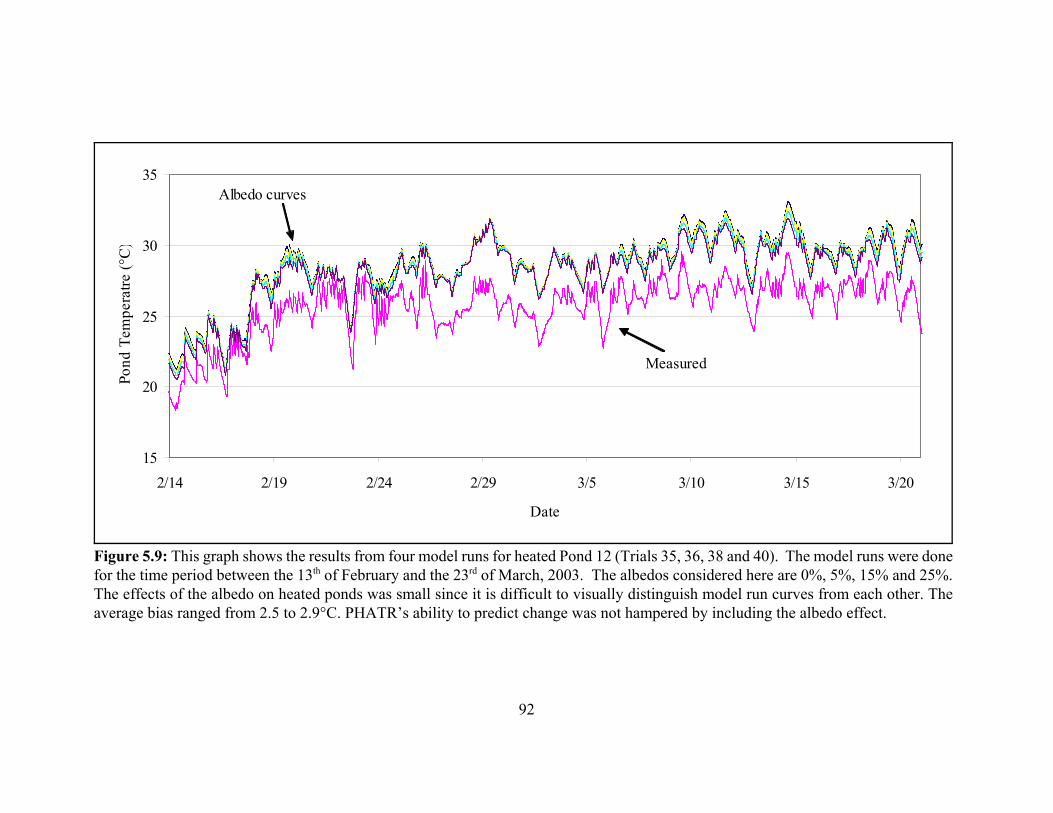
92

15

20

25

30

35

2/14 2/19 2/24 2/29 3/5 3/10 3/15 3/20

Date

Pond

Tem

pera

tre (°

C)

Albedo curves

Measured

Figure 5.9: This graph shows the results from four model runs for heated Pond 12 (Trials 35, 36, 38 and 40). The model runs were donefor the time period between the 13th of February and the 23rd of March, 2003. The albedos considered here are 0%, 5%, 15% and 25%.The effects of the albedo on heated ponds was small since it is difficult to visually distinguish model run curves from each other. Theaverage bias ranged from 2.5 to 2.9°C. PHATR’s ability to predict change was not hampered by including the albedo effect.

93

(Anonymous, 1952) had, on average, an average bias of -1.5°C Because the PHATR Version1.0 over-predicted the pond temperature, using Penman’s Equation might be more appropriatethan using the Lake Hefner Equation, especially when considering heated ponds. The bias for aheated pond run, using wind speed data recorded at 3 meters and using the Penman Equation,was 1.3°C, as opposed to 2.9 for the same output data using the Lake Hefner Equation. Forunheated ponds, the absolute average bias generated by the Penman Equation was greater (-0.7°C) than that generated by the Lake Hefner Equation (0.3°C). Although it might beadvantageous to use Penman’s Equation for heated ponds, using it for unheated ponds couldcause the model to under-predict pond temperature.

The average bias for model runs for unheated ponds using wind speed at 3 meters was 0.125°C. In Chapter 4, the average bias for unheated model runs was 0.5°C. The use of differentequations to estimate evaporation confirmed that PHATR was estimating the order of magnitudeof evaporation energy losses properly. Consequently, if any large errors were present in theequations used by PHATR Version 1.0, it seems less likely they were caused by the Lake HefnerEquation.

5.5.2.2 Convection Coefficient

Not unlike the empirical equations used to estimate evaporation losses, the empirical equationsused to estimate heat transfer losses yielded results similar to each other (see Table 5.4). Thisagain supports the idea that PHATR Version 1.0 was properly estimating the rate of convectiveheat transfer to an order of magnitude.

The standard deviation for the biases and the correlation coefficient were similar betweentreatments. The average difference between the standard deviation for Watmuff et al.’s Equationand the standard deviation for Nusselt number correlations was 0.075°C. The average differencebetween the correlation coefficient for Watmuff et al.’s Equation and the correlation coefficientfor Nusselt number correlations was 0.0075. This suggests that using either set of empiricalequations did not affect PHATR’s ability to predict change.

However, there was a pronounced difference when considering the model’s bias for heatedponds. (The average difference between the average bias for Watmuff et al.’s Equation and theaverage bias for Nusselt number correlations was 0.83°C.) This was especially true for themodel run for a heated pond (wind speed measurements taken at 3 meters), where the differencebetween the average biases was 2.1°C. Because the Nusselt number correlations increasedPHATR’s tendency to over-predict, Watmuff et al.’s Equation should be used.

Equation 3.58 (Watmuff et al., 1977) was preferred to the Nusselt number correlations for otherreasons. The Nusselt number correlations represent 30 lines of computer code whereasEquation 3.58 represents only 1 line of code. Consequently, fixing and verifying PHATR’sseries of calculations was much simpler when using Equation 3.58. Furthermore, using theNusselt number correlations required more input data. The additional required data sets werelocal atmospheric pressure (used in the ideal gas law when calculating the density of air) and

94

wind direction (used to determine the characteristic length of heat transfer for the correlations). The user also needed to know the orientation of his pond, which may not have been convenient. More input data meant there was a greater chance there would be more errors in the input andoutput data. For the user, finding more data was not convenient. Since both equations wereempirical, and since both equations were roughly equivalent in predicting pond temperature(although more experimenting is required), the simpler Equation 3.58 should be used.

5.5.2.3 Effects of Height for Wind Speed Measurements

There was a difference in the bias when using wind speeds measured at different heights. Theaverage bias for trials where the wind speed was measured at the pond surface was -4.85°C. Theaverage bias for trials where the wind speed was measured 3 meters from the ground into the airwas 1.61°C. Therefore, the using the wind speed at the surface caused the model to under-predict pond temperature.

This might be caused by Equation 3.73, the equation used to calculate an equivalent wind speedfor different heights. The equation assumes that there is an exponential profile for the velocityboundary layer. However, near the surface, this is might not be true because of the roughness ofthe surface or because of the presence of obstacles (such as levees). By assuming that the heightof the anemometer is where the wind speed is measured (33 cm or 1.1 feet), the wind speedmeasured at this height needs to be multiplied to a correction factor of (ln 13/ln 1.1) or 27, whichis not reasonable if wind speeds measured near the pond surface ranged from 0 to 7.29 m/s (0 to16.3 mph), as it did between February 13th and March 23st, 2003 on Pond 12. Applying thecorrection factor would yield wind speeds up to 196 m/s (440 mph).

An other cause for the large differences in bias might be because wind speeds at different heightspoorly correlate. Upon examining the wind speed data for different heights, the correlationcoefficient between these two data sets was r = 0.76. Consequently, both data sets, somewhatrelated, should have yielded similar results if Equation 3.73 was not used. For this reason,Equation 3.73, and not the data, was probably the cause of the error for the poor model outputs,for model runs using wind speed data collected near the water surface.

5.5.3 Extinction Coefficient

The strong negative correlation coefficients in Table 5.5 (average = -0.96, range -0.83 to -0.999)could allow for the following assumptions to be made:

• the Bouger-Beer Law, for these ponds, is valid and can be used to determine theextinction coefficient.• the pond turbidity can be assumed to be constant with depth, probably because of theaerators, which were constantly running and continuously mixing the suspendedsediments.

95

However, results from the pairwise comparison do not support the conclusion that the extinctioncoefficient is the same throughout the pond. Results showed that there were significantdifferences between the extinction coefficient measured at the aerator and in the middle of thepond (p = 0.017) and between the extinction coefficient measured at the middle and at the standpipe (p = 0.034). There was no difference between the extinction coefficient measured at theaerator and at the standpipe (p = 0.48). This seems contradictory but might be explained withthe results from the pairwise comparisons of the extinction coefficient between ponds.

Pond 13, in the spring time, had significantly different extinction coefficients from all other pond(p < 0.001 for all cases; see Figure 5.8). Furthermore, upon examining the data collected withinPond 13, the extinction coefficient had variations within the pond. The difference between theextinction coefficient at the aerator and the extinction coefficient at the middle of the pond wassignificant (difference = 0.00931 mm-1, p = 0.01735). The difference between the extinctioncoefficient at the outlet and the extinction coefficient at the middle of the pond was alsosignificant (difference = 0.007952 mm-1, p = 0.0297). There was no significant differencebetween the extinction coefficient measured at the aerator or at the discharge (difference =0.00136; p = 0.35245).

There were no significant differences in the extinction coefficients between the ponds (F2,18 =0.65, p = 0.266) or within the ponds (F2,18 = 1.31, p = 0.1469) if the extinction coefficientcollected from Pond 13 during the spring was excluded from the statistical analysis. Therefore,results from Pond 13 in the spring time affected the pairwise comparisons of the extinctioncoefficient within a pond.

Unlike the other ponds or Pond 13 in the fall, Pond 13 in the spring was noticeably more brownand muddy. This might explain the greater extinction coefficients observed in this pond.

5.5.4 Albedo

The main purpose for including the albedo in the model was to reduce the consistently over-predictive bias. This would have been especially beneficial for heated model runs, where thebias was larger. However, the albedo’s effects were more pronounced in unheated ponds. Table5.7 shows the effects of varying the bias by 25%. Although varying the albedo lowered, onaverage, the bias by 0.95°C, varying the albedo for heated ponds only lowered the bias by0.45°C. Therefore, the albedo was not responsible for the large bias calculated for heated ponds.

The correlation coefficient for all runs was over 0.94. This shows that including the influence ofan albedo does not affect the model’s ability to predict change.

Recommending an albedo to be used in subsequent model runs might be difficult. The results inTable 5.6 make it unclear which albedo should be used. Clearly, the empirical equations used bythe model to predict evaporation and surface convection had an effect on the bias. Unfortunately,this effect cannot be separated from the albedo’s influence on the results.

96

Table 5.7: Differences in average bias between model runs with an albedo of 0 and 25% rangedfrom 0.4 to 1.3°C.

Pond Treatment Change in Bias (°C)3 Unheated 1.03 Unheated 1.212 Heated 0.412 Heated 0.513 Unheated 1.213 Unheated 1.3

Therefore, an albedo will be recommended for a model using Penman’s equation and an otheralbedo will be recommended for a model using the Lake Hefner Equation. When considering unheated ponds, Trial 43 was the only trial using Penman’s equation wherethe average bias was 0°C. For Trials 17 through 22, increasing the albedo increased the model’serror. Therefore, because Penman’s equation, when compared with the Lake Hefner equation,has a tendency to over-estimate evaporation losses, a low albedo should be used (5%).

Alternately, for a version of PHATR using the Lake Hefner equation, a higher albedo might benecessary. Trials 24 (albedo = 5%) and 52 (albedo = 25%) yielded results with an average biasof 0°C. Using an average of albedo of 15% causes the error for both ponds to be within a degreeof the measured pond temperature (Trial 26, bias = -0.5°C; Trial 50, bias = 0.6°C).

5.6 Conclusions

Ways to improve PHATR Version 1.0 were explored with mixed success.

The heat and mass transfer coefficients could not be determined using the heat and mass transferanalogy. Results yielded negative heat and mass transfer coefficient values, which is physicallyimpossible. These negative values were caused in part by the inaccuracy of thermocouples tomeasure the pond temperature to one one-hundredth of a degree Celsius. Accurate temperaturesensing devices would be needed in order to determine both transport coefficients.

Comparisons were made between the various empirical equations used to estimate evaporationlosses over bodies of water. All equations yielded similar results. Therefore, the size ofevaporative energy losses was probably properly estimated. Equation 3.67 (Penman, 1948)predicted greater evaporation losses whereas equation 3.70 (Piedrahita, 1991) predicted smallerevaporation losses. Because the model already closely predicted the temperature for unheatedponds, using the Penman equation would cause the model to under-predict the pond temperaturewithout the effects of an albedo. Therefore, the Lake Hefner equation is probably the bestequation to use to estimate evaporative heat losses for heated and unheated ponds (volume = 400m3).

97

Comparisons were also made between Nusselt number correlations and Equation 3.58 (Watmuffet al, 1977). Both methods yielded similar results and therefore, the size of the convective heattransfer coefficient was probably properly estimated. However, because the Nusselt numbercorrelations are more complex and require more input data without being more accurate,Equation 3.58 should be used.

When choosing wind speed data for PHATR’s input, wind speeds recorded at 3 meters proved toyield better results. Using wind speeds recorded at the water surface caused the model toconsistently under-predict the pond temperature by 4.3 to 5.5°C. This is probably becauseEquation 3.73 cannot be used for converting wind speeds recorded close to the water surface.

The average extinction coefficient for the warm water ponds was 0.013 mm-1, with valuesranging from 0.004 to 0.031 mm-1. This average includes the data from the more turbid Pond 13in the spring of 2003. The extinction coefficients for pond 13 were significantly different fromthe extinction coefficient measured in all other ponds. Statistically similar extinctioncoefficients can be explained by the aerators constantly mixing the pond water.

The albedo was estimated empirically using a modified version of PHATR. The method waspartially successful although not conclusive. Because of the difficulty of either theoreticallycalculating or measuring this parameter, the method used was seen as the only realisticalternative. Consequently, the albedo’s value is greatly affected by any inaccuracies inherent inthe model, such as inaccuracies associated with empirical equations. Therefore, two albedoswere calculated. An albedo of 5% is to be used in models using Equation 3.67 (Penman, 1948)to estimate evaporation energy losses, whereas an albedo of 15% is to be used in models usingEquation 3.71, the Lake Hefner equation (Anonymous, 1952). Including the effects of an albedodid not impair PHATR’s ability to predict changes in pond temperature. This was reflected inthe high correlation coefficient values in the results.

For all the trials modeling unheated ponds, the average of the average bias was -0.88°C. For allthe trials modeling heated ponds, the average of the average bias was 0.79°C. Varying thealbedo, convection and evaporation did not further correct the model when predicting pondtemperature for heated ponds. This supports the conclusion in Chapter 4 that the average biasesfor heated ponds were larger than the average biases for unheated ponds because the flow rate ofwarm or cool water cannot be measured accurately.

98

CHAPTER 6: SENSITIVITY ANALYSIS

6.1 Introduction

PHATR, a computer model used to predict the temperature for small well mixed ponds (fulldescription of the model can be found in Chapter 4), uses data inputs of various kinds. The datadescribes the weather, the flow of water into the pond and the physical characteristics of thepond itself. How the data affects the model output can be studied with a sensitivity analysis.

A sensitivity analysis, defined by Saltelli (2000) is “the study of how the variation in the outputof a model (numerical or otherwise) can be apportioned, qualitatively or quantitatively, todifferent sources of variation, and of how the given model depends upon the information fed intoit.” For PHATR, the sensitivity analysis revealed which changes in the input caused greater orlesser changes in the output. The sensitivity analysis also identified certain scenarios wherevarying a certain input variable had a counter-intuitive effect on the results.

6.2 Materials and Methods

A type sensitivity analysis was performed For such an analysis, a standard model run, with fixedinput variables, is compared to trial model runs. For each trial, only one input variable in thestandard model run was changed by a pre-determined increment. By comparing changes in theoutput to changes in the input, the model’s sensitivity can be gaged.

The standard model run consisted of running PHATR Version 1.2 for 2 hypothetical days for ahypothetical pond with dimensions 1 meter x 1 meter x 1 meter (pond characteristics shown inTable 6.1).

Table 6.1: These characteristics for a hypothetical pond were used for the sensitivity analysis ofPHATR, Version 1.2.

Pond Characteristic Value

Initial Pond Temperature 20°C

Pond Volume 1 m3

Pond Area 1 m2

Flow rate of warm water 0 m3/s

Time period considered for the model run 2 days (172800 seconds)

The weather during these 2 hypothetical days was clear (no clouds) with an average airtemperature of 20°C. The air temperature varied sinusoidally. The daytime high, 25°C,occurred at 14:00 (2 P.M.) and the daytime low, 15°C, occurred at 2:00 (2 A.M.). Solar radiation

99

varied sinusoidally between 6:00 and 18:00 (6 A.M. and 6 P.M.), the maximum (1355 W/m2)occurring at 12:00 (noon). The relative humidity was set constant at 90%. There was no wind(wind speed = 0 m/s). All weather variables for the standard are shown in Table 6.2.

There was no warm or cool water flowing in the pond for the standard model run. The pondtemperature at the start of the two day period was 20°C.

Table 6.2: These weather variables described the standard weather used for the sensitivity analysisof PHATR, Version 1.2. For the equations used to describe solar radiation and air temperature, t =time in hours. Also note that between 18:00 and 6:00, solar radiation is equal to 0 W/m2.

Weather Variable Value

Air Temperature( )

20 58

12+

−

sinπ t

Relative Humidity 90%

Solar Radiation( )

13556

12sin

π t −

Wind Speed 0 m/s

PHATR Version 1.2, a more “user-friendly” version of PHATR Version 1.0, was used to performall the model runs. The time step used was 10 minutes and all model runs simulated a period of2 days.

For each model run, one variable was changed while keeping all other weather conditions at theirhypothetical standard value (see Table 6.3 for the exact nature of each variation). Four variableswere changed:

• average air temperature • solar radiation • wind speed • flow rate of warm water (36°C).

The average air temperature was set at either 0, 10, 15, 20, 25, 30 or 40°C. Diurnal fluctuationswere modeled as a sinusoidal function with an amplitude of 5°C. The daytime high occurs at14:00 and the night time low occurs at 2:00.

The solar radiation was varied by 0%, -25%, -50%, -75% and -100% of the standard solarradiation value predicted by the equation in Table 6.2.

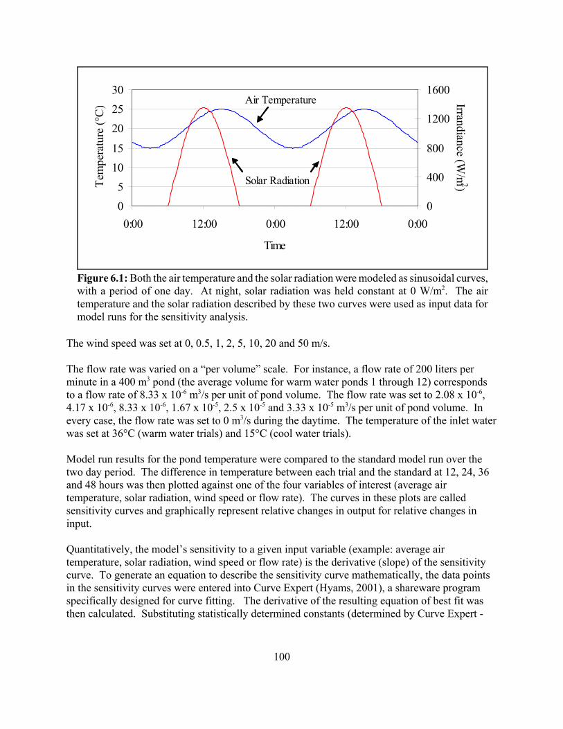
100

05

1015

202530

0:00 12:00 0:00 12:00 0:00

Time

Tem

pera

ture

(°C

)

0

400

800

1200

1600Irrandiance (W

/m2)Solar Radiation

Air Temperature

Figure 6.1: Both the air temperature and the solar radiation were modeled as sinusoidal curves,with a period of one day. At night, solar radiation was held constant at 0 W/m2. The airtemperature and the solar radiation described by these two curves were used as input data formodel runs for the sensitivity analysis.

The wind speed was set at 0, 0.5, 1, 2, 5, 10, 20 and 50 m/s.

The flow rate was varied on a “per volume” scale. For instance, a flow rate of 200 liters perminute in a 400 m3 pond (the average volume for warm water ponds 1 through 12) correspondsto a flow rate of 8.33 x 10-6 m3/s per unit of pond volume. The flow rate was set to 2.08 x 10-6,4.17 x 10-6, 8.33 x 10-6, 1.67 x 10-5, 2.5 x 10-5 and 3.33 x 10-5 m3/s per unit of pond volume. Inevery case, the flow rate was set to 0 m3/s during the daytime. The temperature of the inlet waterwas set at 36°C (warm water trials) and 15°C (cool water trials).

Model run results for the pond temperature were compared to the standard model run over thetwo day period. The difference in temperature between each trial and the standard at 12, 24, 36and 48 hours was then plotted against one of the four variables of interest (average airtemperature, solar radiation, wind speed or flow rate). The curves in these plots are calledsensitivity curves and graphically represent relative changes in output for relative changes ininput.

Quantitatively, the model’s sensitivity to a given input variable (example: average airtemperature, solar radiation, wind speed or flow rate) is the derivative (slope) of the sensitivitycurve. To generate an equation to describe the sensitivity curve mathematically, the data pointsin the sensitivity curves were entered into Curve Expert (Hyams, 2001), a shareware programspecifically designed for curve fitting. The derivative of the resulting equation of best fit wasthen calculated. Substituting statistically determined constants (determined by Curve Expert -

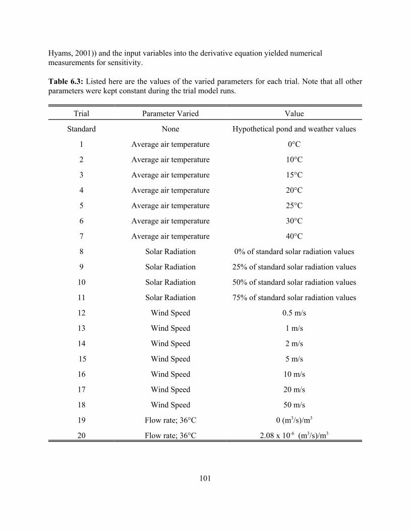
101

Hyams, 2001)) and the input variables into the derivative equation yielded numericalmeasurements for sensitivity.

Table 6.3: Listed here are the values of the varied parameters for each trial. Note that all otherparameters were kept constant during the trial model runs.

Trial Parameter Varied Value

Standard None Hypothetical pond and weather values

1 Average air temperature 0°C

2 Average air temperature 10°C

3 Average air temperature 15°C

4 Average air temperature 20°C

5 Average air temperature 25°C

6 Average air temperature 30°C

7 Average air temperature 40°C

8 Solar Radiation 0% of standard solar radiation values

9 Solar Radiation 25% of standard solar radiation values

10 Solar Radiation 50% of standard solar radiation values

11 Solar Radiation 75% of standard solar radiation values

12 Wind Speed 0.5 m/s

13 Wind Speed 1 m/s

14 Wind Speed 2 m/s

15 Wind Speed 5 m/s

16 Wind Speed 10 m/s

17 Wind Speed 20 m/s

18 Wind Speed 50 m/s

19 Flow rate; 36°C 0 (m3/s)/m3

20 Flow rate; 36°C 2.08 x 10-6 (m3/s)/m3

102

Table 6.3 continued

Trial Parameter Varied Value

21 Flow rate; 36°C 4.17 x 10-6 (m3/s)/m3

22 Flow rate; 36°C 8.33 x 10-6 (m3/s)/m3

23 Flow rate; 36°C 1.67 x 10-5 (m3/s)/m3

24 Flow rate; 36°C 2.5 x 10-5 (m3/s)/m3

25 Flow rate; 36°C 3.33 x 10-5 (m3/s)/m3

26 Flow rate; 15°C 2.08 x 10-6 (m3/s)/m3

27 Flow rate; 15°C 4.17 x 10-6 (m3/s)/m3

28 Flow rate; 15°C 8.33 x 10-6 (m3/s)/m3

29 Flow rate; 15°C 1.67 x 10-5 (m3/s)/m3

30 Flow rate; 15°C 2.5 x 10-5 (m3/s)/m3

31 Flow rate; 15°C 3.33 x 10-5 (m3/s)/m3

6.3 Results and Analysis

6.3.1 Variations in the average air temperature

Lowering the average air temperature resulted in relatively lower pond temperatures at the end ofthe two day period (see Figure 6.2). For instance, the pond temperature, after being exposed toan average air temperature of 0°C for 48 hours, was 26.7°C, 6.3°C below the standard model runpond temperature. Alternately, increasing the average air temperature raised the pondtemperature. As an example, the pond temperature, after being exposed to 40°C air for 48 hours,was 40.5°C, 7.5°C above the standard model run pond temperature. As time progressed, theabsolute difference between the standard temperature and the resulting trial temperatureincreased. Therefore, the model’s sensitivity to changes in air temperature were dependant ontime, as shown by the different slopes for the sensitivity curves in Figure 6.2b.

A linear regression was applied to each curve in Figure 6.2b. The correlation coefficients andthe slopes for each curve are shown in Table 6.4. As the time step increased from 12 to 48hours, the slope also increased from 0.097 °C/°C to 0.48 °C/°C. Because the slope of a line isalso the derivative of a line, and because the curves in Figure 6.2 were lines (r = 0.999 for alltime steps), the slopes in Table 6.4 were measurements of the model’s sensitivity.

103

0

5

10

15

20

25

30

35

40

45

0:00 4:00 7:59 12:00 16:00 19:59 0:00 4:00 7:59 12:00 16:00 19:59 0:00

Time

Pond

tem

pera

ture

(°C

) 40°C30°C

0°C

25°C20°C15°C10°C

Figure 6.2a: These curves describe how the pond temperature changed over 2 days of hypothetical weather. The temperature labelson the right hand side of the graph were the average air temperature for the sensitivity analysis trials. Cooler air temperatures causedthe pond temperature to decrease with respect to the standard (shown here as the 20°C curve). Warmer air temperatures caused the pondtemperature to increase with respect to the standard.

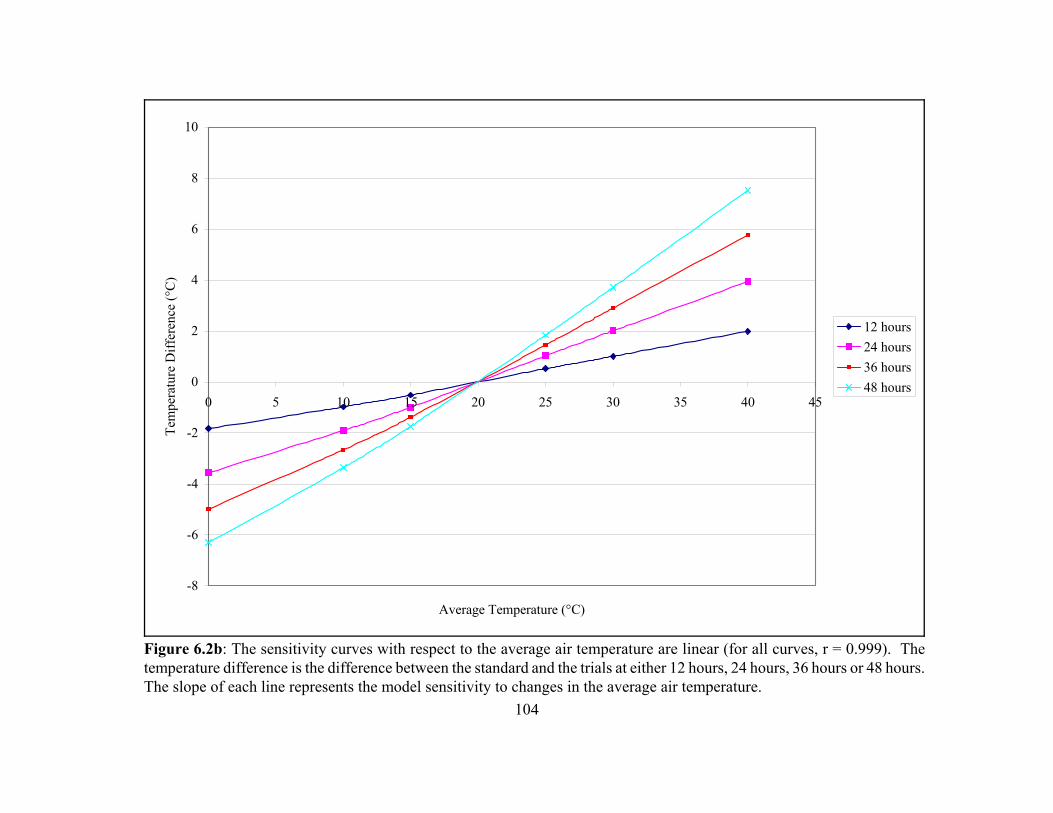
104

-8

-6

-4

-2

0

2

4

6

8

10

0 5 10 15 20 25 30 35 40 45

Average Temperature (°C)

Tem

pera

ture

Diff

eren

ce (°

C)

12 hours24 hours36 hours48 hours

Figure 6.2b: The sensitivity curves with respect to the average air temperature are linear (for all curves, r = 0.999). Thetemperature difference is the difference between the standard and the trials at either 12 hours, 24 hours, 36 hours or 48 hours.The slope of each line represents the model sensitivity to changes in the average air temperature.

105

Table 6.4: The sensitivity curves in Figure 6.2b were statistically quantified with linear regressionparameters. Note how the slope (sensitivity) increased with time.

Time (hr) Slope (°Coutput/°Cinput) Correlation coefficient ( r)

12 0.097 0.999

24 0.190 0.999

36 0.271 0.999

48 0.348 0.999

To determine if any relationship existed between the slope of each sensitivity curve and time, theslopes were plotted against time (see Figure 6.4). The slopes were found to vary linearly withtime (r = 0.999). The rate of change of the slopes was 0.00695 °C/°C/hr and the intercept forthis line was 0.0178 °C/°C.

This information is useful when determining the effects of measurement errors or poor data onthe model’s output. For instance, suppose an error of 5°C was present in the air temperature dataset. The error was present for 30 hours. What was the corresponding error in the output?

The model’s sensitivity to air temperature was found to vary with time. For a 30 hour period, thesensitivity was:

0 00695 30 0 0178

0 2285

0 0

0

. .

.

CC

CC

CC

o o

o

hr hrs× +

=

A 5°C error in input translates into an output error of 1.1425°C.

6.3.2 Variations in Solar Radiation

Decreasing the amount of incident solar radiation decreased the pond temperature (see Figure6.5). This made sense since solar energy was found to be the major energy transfer mechanismduring the day, accounting for as much as 55% of all energy vectors (see chapter 4). After 48hours, the pond temperature increased for all trials except for trial 8 where there was no solarradiation. In this case, the pond temperature steadily decreased almost linearly ( r = -0.955) by1.46°C.

The model’s sensitivity to changes in solar radiation was quantified by calculating the slopes ofthe curves in Figure 6.6. All curves in Figure 6.6 had correlation coefficients above 0.999. Theintercepts for each curve was also calculated (results shown in Table 6.5).

106

0

0.05

0.1

0.15

0.2

0.25

0.3

0.35

0.4

0 10 20 30 40 50 60

Time (hours)

The

Mod

el's

Sens

itivi

ty to

the

Ave

rage

Air

Tem

pera

ture

Cha

nges

(°C

/°C

)

Figure 6.3: The model’s sensitivity to the average air temperature increased with time at a rate of 0.00695 (°C/°C)/hr. The slope ofeach sensitivity curve was plotted against time to generate this graph.

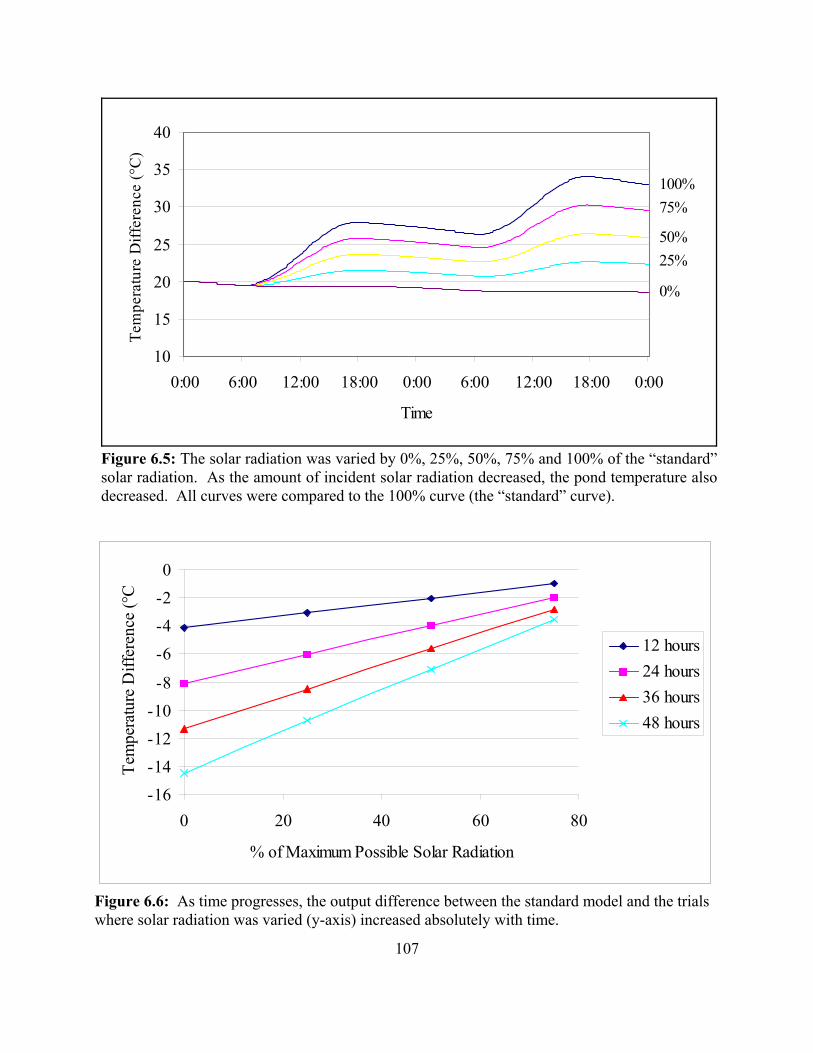
107

-16-14-12-10

-8

-6-4-20

0 20 40 60 80

% of Maximum Possible Solar Radiation

Tem

pera

ture

Diff

eren

ce (°

C

12 hours24 hours36 hours48 hours

Figure 6.6: As time progresses, the output difference between the standard model and the trialswhere solar radiation was varied (y-axis) increased absolutely with time.

10

15

20

25

30

35

40

0:00 6:00 12:00 18:00 0:00 6:00 12:00 18:00 0:00

Time

Tem

pera

ture

Diff

eren

ce (°

C)

100%75%

0%

25%50%

Figure 6.5: The solar radiation was varied by 0%, 25%, 50%, 75% and 100% of the “standard”solar radiation. As the amount of incident solar radiation decreased, the pond temperature alsodecreased. All curves were compared to the 100% curve (the “standard” curve).

108

(6.1a)

(6.1b)

(6.1c)

(6.2)

Table 6.5: These are the linear regression parameters for the sensitivity curves in Figure 6.3. Again, the slope and the intercepts varied linearly with time.

Time (hours) Slope (°C / %) Intercept (°C)

12 0.0413 -4.13

24 0.0812 -8.08

36 0.1138 -11.32

48 0.1455 -14.41

Again, the slope and the intercepts of each curve changed linearly with time. (The correlationcoefficient for the rate of change in the slope was 0.998. The correlation coefficient for the rateof change in the intercept was -0.998.) A linear regression was applied to both the slopes andthe intercepts to determine how the sensitivity changed with time. Results are shown in Figure6.7. The equations for the slope and the intercept with respect to time are:

ξ

ξ

ξ φ ξ

slope

ercept

slope ercept

t

t

T

= +

= − −

= +

0 0029 0 0091

0 284 0 9627

. .

. .int

int∆

where N is the fraction of solar radiation set for the trial runs and )T is the difference between the standard pond temperature andthe trial pond temperature for a fixed time (°C),

The last equation, Equation 6.1c, is the equation used to determine the model’s sensitivity withrespect to solar radiation.

The sensitivity curves in Figures 6.3 and 6.6 were straight lines in part because of the solution tothe governing differential equation but also in part because of the times chosen to examine themodel’s sensitivity. Consider the following simplified version of Equation 3.4, the energybalance equation, where qsolar is the only flux of energy present. In other words, energy transfermechanisms associated with convection, conduction, evaporation, long wave radiation or bulkmovements of mass are negligible. Equation 3.4 then simplifies to Equation 6.2:

dEdt

qpond

solar

=

109

y = -0.284x - 0.9627R2 = 0.9965

y = 0.0029x + 0.0091R2 = 0.9969

00.020.040.060.080.1

0.120.140.16

0 10 20 30 40 50 60

Time (hours)

Slop

e (°

C/W

)

-16-14-12-10-8-6-4-20

Intercept (°C)

Figure 6.7: The slopes and the intercepts for the sensitivity curves varied linearly in time, as shownhere. The slopes of the sensitivity curves varied according to the ascending curve with the givenequation while the intercepts of the sensitivity curves along the descending curve.

(6.3a)

(6.3b)

(6.4)

where E is the internal pond energy (Joules),

qsolar is the solar radiation (Joules/hour) t is time (hour).

Knowing that (dE/dt)pond and qsolar can be substituted with the following:

dEdt

cdTdtp= ∀ρ

qt

solar = −

1355

12φ

πcos

where D is the density of water (kg/m3), cp is the specific heat of water (J/kg°C), œ is the pond volume (m3) andT is the pond temperature (°C)

Equation 6.2 becomes:

ρ φπ

cdTdt

tp∀ = −

1355

12cos

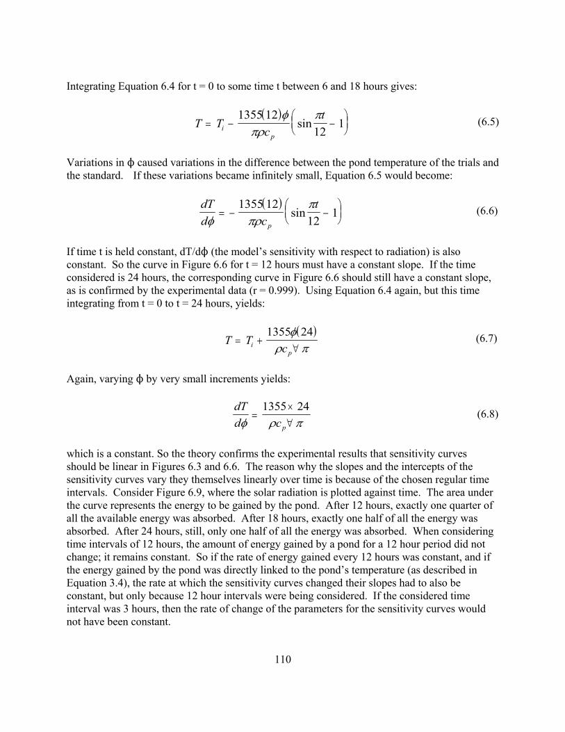
110

(6.5)

(6.6)

(6.7)

(6.8)

Integrating Equation 6.4 for t = 0 to some time t between 6 and 18 hours gives:

( )T T

ct

ip

= − −

1355 1212

1φ

πρπ

sin

Variations in N caused variations in the difference between the pond temperature of the trials andthe standard. If these variations became infinitely small, Equation 6.5 would become:

( )dTd c

t

pφ πρπ

= − −

1355 1212

1sin

If time t is held constant, dT/dN (the model’s sensitivity with respect to radiation) is alsoconstant. So the curve in Figure 6.6 for t = 12 hours must have a constant slope. If the timeconsidered is 24 hours, the corresponding curve in Figure 6.6 should still have a constant slope,as is confirmed by the experimental data (r = 0.999). Using Equation 6.4 again, but this timeintegrating from t = 0 to t = 24 hours, yields:

( )T T

cip

= +∀

1355 24φρ π

Again, varying N by very small increments yields:

dTd cpφ ρ π

=×∀

1355 24

which is a constant. So the theory confirms the experimental results that sensitivity curvesshould be linear in Figures 6.3 and 6.6. The reason why the slopes and the intercepts of thesensitivity curves vary they themselves linearly over time is because of the chosen regular timeintervals. Consider Figure 6.9, where the solar radiation is plotted against time. The area underthe curve represents the energy to be gained by the pond. After 12 hours, exactly one quarter ofall the available energy was absorbed. After 18 hours, exactly one half of all the energy wasabsorbed. After 24 hours, still, only one half of all the energy was absorbed. When consideringtime intervals of 12 hours, the amount of energy gained by a pond for a 12 hour period did notchange; it remains constant. So if the rate of energy gained every 12 hours was constant, and ifthe energy gained by the pond was directly linked to the pond’s temperature (as described inEquation 3.4), the rate at which the sensitivity curves changed their slopes had to also beconstant, but only because 12 hour intervals were being considered. If the considered timeinterval was 3 hours, then the rate of change of the parameters for the sensitivity curves wouldnot have been constant.

111

0

500

1000

1500

0:00 12:00 0:00 12:00 0:00

Time

Sola

r Rad

iatio

n (W

/m2 ) .

Figure 6.9: By considering the pond temperature every 12 hours, thesame exact amount of solar radiation (one quarter of the two day total)was absorbed by the pond, causing the slopes and the intercepts of thesensitivity curves in Figure 6.6 to vary linearly with time.

6.3.3 Variations in WindSpeed

Two energy vectors aredirectly affected bychanges in wind speed:heat convection at thepond surface andevaporation. However,increasing the wind speeddoes not necessarily meanconvection or evaporationare more important. Bothconvection andevaporation are alsoaffected by their respectivegradients, the true drivingforce behind these energytransfer mechanisms. Inthe case of convection, thetemperature gradientbetween the air and the water surface drives this transport phenomena. In the case ofevaporation, the vapor pressure gradient between the water surface and the air is the drivingforce. Because increasing the wind speed can change the temperature of the water, the gradientsfor heat and mass transfer also change and consequently, the size of the convection andevaporation vectors also change counter intuitively. Increasing the wind speed also had different effects dependant on the time of day. At noon onday 2, increasing the wind speed from 0 to 5 m/s caused the pond temperature to decrease from30.1°C to 25.4°C, mainly because the rate of energy lost by evaporation increased from 46 W to110 W. However, this drop in pond temperature also decreased the vapor pressure of the water. Warmer water has more internal energy so more water vapor can evaporate from the watersurface. Consequently, warmer water has a greater vapor pressure (the pressure of the waterevaporating into the air) than cooler water. By cooling the pond water (and reducing the pond’svapor pressure), but keeping the air temperature constant (and keeping the air’s vapor pressureconstant), the pressure gradient which drives evaporation became smaller, because of the largerwind speed. Energy losses due to evaporation decreased when the wind speed was increasedbeyond 5 m/s. For a wind speed of 50 m/s, there was no evaporation because the watertemperature was so low that the water vapor pressure (2.51 kPa) was smaller than the air vaporpressure (2.87 kPa) .

Convection only removed heat from the pond for wind speeds under 10 m/s at noon on Day 2. Because the pond temperature for a wind speed of 10 m/s, 23.3°C, was below the airtemperature, 23.53°C, the air “warmed” the pond. By increasing the wind speed from 10 m/s to

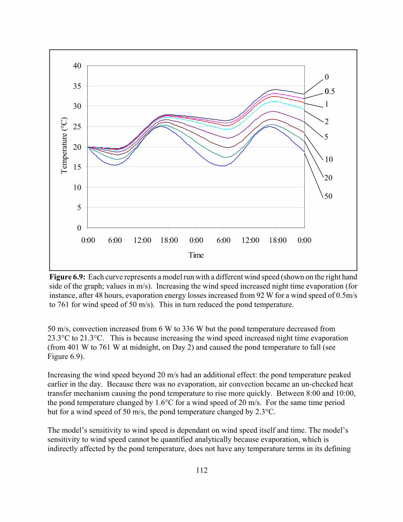
112

0

5

10

15

20

25

30

35

40

0:00 6:00 12:00 18:00 0:00 6:00 12:00 18:00 0:00

Time

Tem

pera

ture

(°C

)0

0.51

2

5

20

50

0

10

Figure 6.9: Each curve represents a model run with a different wind speed (shown on the right handside of the graph; values in m/s). Increasing the wind speed increased night time evaporation (forinstance, after 48 hours, evaporation energy losses increased from 92 W for a wind speed of 0.5m/sto 761 for wind speed of 50 m/s). This in turn reduced the pond temperature.

50 m/s, convection increased from 6 W to 336 W but the pond temperature decreased from23.3°C to 21.3°C. This is because increasing the wind speed increased night time evaporation(from 401 W to 761 W at midnight, on Day 2) and caused the pond temperature to fall (seeFigure 6.9).

Increasing the wind speed beyond 20 m/s had an additional effect: the pond temperature peakedearlier in the day. Because there was no evaporation, air convection became an un-checked heattransfer mechanism causing the pond temperature to rise more quickly. Between 8:00 and 10:00,the pond temperature changed by 1.6°C for a wind speed of 20 m/s. For the same time periodbut for a wind speed of 50 m/s, the pond temperature changed by 2.3°C.

The model’s sensitivity to wind speed is dependant on wind speed itself and time. The model’ssensitivity to wind speed cannot be quantified analytically because evaporation, which isindirectly affected by the pond temperature, does not have any temperature terms in its defining

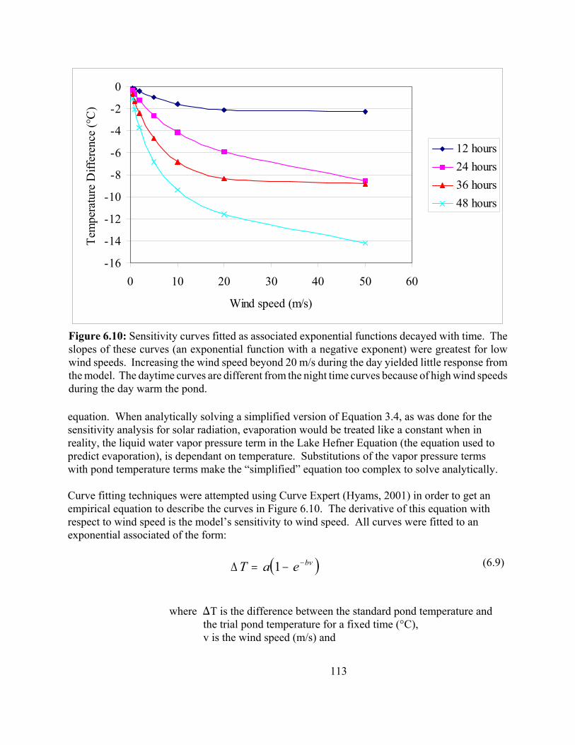
113

-16

-14

-12

-10

-8

-6

-4

-2

0

0 10 20 30 40 50 60

Wind speed (m/s)

Tem

pera

ture

Diff

eren

ce (°

C)

12 hours24 hours36 hours48 hours

Figure 6.10: Sensitivity curves fitted as associated exponential functions decayed with time. Theslopes of these curves (an exponential function with a negative exponent) were greatest for lowwind speeds. Increasing the wind speed beyond 20 m/s during the day yielded little response fromthe model. The daytime curves are different from the night time curves because of high wind speedsduring the day warm the pond.

(6.9)

equation. When analytically solving a simplified version of Equation 3.4, as was done for thesensitivity analysis for solar radiation, evaporation would be treated like a constant when inreality, the liquid water vapor pressure term in the Lake Hefner Equation (the equation used topredict evaporation), is dependant on temperature. Substitutions of the vapor pressure termswith pond temperature terms make the “simplified” equation too complex to solve analytically.

Curve fitting techniques were attempted using Curve Expert (Hyams, 2001) in order to get anempirical equation to describe the curves in Figure 6.10. The derivative of this equation withrespect to wind speed is the model’s sensitivity to wind speed. All curves were fitted to anexponential associated of the form:

( )∆T a e bv= − −1

where )T is the difference between the standard pond temperature andthe trial pond temperature for a fixed time (°C), v is the wind speed (m/s) and

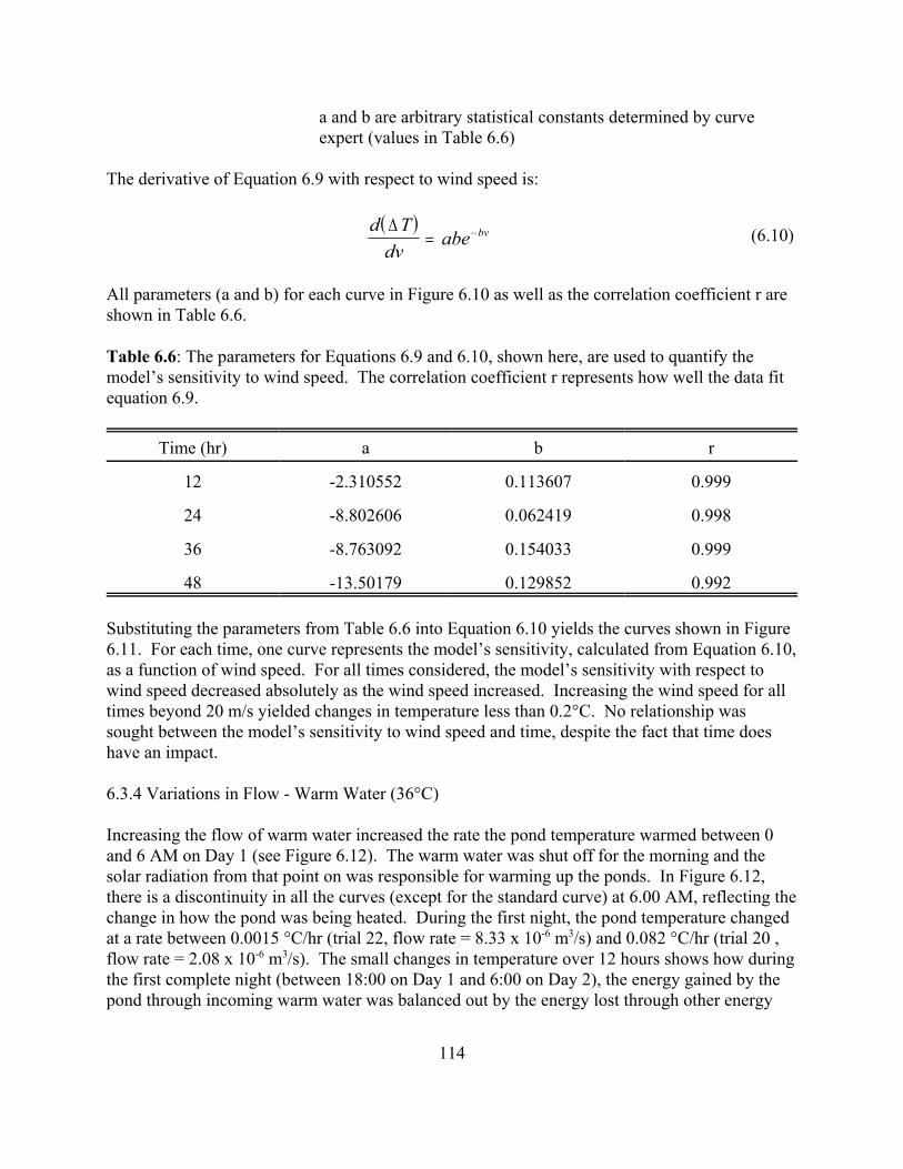
114

(6.10)

a and b are arbitrary statistical constants determined by curveexpert (values in Table 6.6)

The derivative of Equation 6.9 with respect to wind speed is:

( )d Tdv

abe bv∆= −

All parameters (a and b) for each curve in Figure 6.10 as well as the correlation coefficient r areshown in Table 6.6.

Table 6.6: The parameters for Equations 6.9 and 6.10, shown here, are used to quantify themodel’s sensitivity to wind speed. The correlation coefficient r represents how well the data fitequation 6.9.

Time (hr) a b r

12 -2.310552 0.113607 0.999

24 -8.802606 0.062419 0.998

36 -8.763092 0.154033 0.999

48 -13.50179 0.129852 0.992

Substituting the parameters from Table 6.6 into Equation 6.10 yields the curves shown in Figure6.11. For each time, one curve represents the model’s sensitivity, calculated from Equation 6.10,as a function of wind speed. For all times considered, the model’s sensitivity with respect towind speed decreased absolutely as the wind speed increased. Increasing the wind speed for alltimes beyond 20 m/s yielded changes in temperature less than 0.2°C. No relationship wassought between the model’s sensitivity to wind speed and time, despite the fact that time doeshave an impact.

6.3.4 Variations in Flow - Warm Water (36°C)

Increasing the flow of warm water increased the rate the pond temperature warmed between 0and 6 AM on Day 1 (see Figure 6.12). The warm water was shut off for the morning and thesolar radiation from that point on was responsible for warming up the ponds. In Figure 6.12,there is a discontinuity in all the curves (except for the standard curve) at 6.00 AM, reflecting thechange in how the pond was being heated. During the first night, the pond temperature changedat a rate between 0.0015 °C/hr (trial 22, flow rate = 8.33 x 10-6 m3/s) and 0.082 °C/hr (trial 20 ,flow rate = 2.08 x 10-6 m3/s). The small changes in temperature over 12 hours shows how duringthe first complete night (between 18:00 on Day 1 and 6:00 on Day 2), the energy gained by thepond through incoming warm water was balanced out by the energy lost through other energy

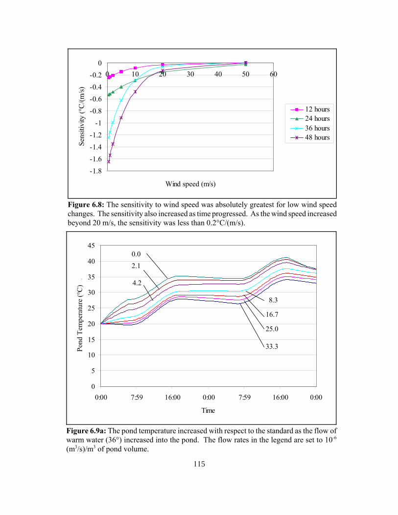
115

-1.8-1.6-1.4-1.2

-1-0.8-0.6-0.4-0.2

00 10 20 30 40 50 60

Wind speed (m/s)

Sens

itivi

ty (°

C/(m

/s)

12 hours24 hours36 hours48 hours

Figure 6.8: The sensitivity to wind speed was absolutely greatest for low wind speedchanges. The sensitivity also increased as time progressed. As the wind speed increasedbeyond 20 m/s, the sensitivity was less than 0.2°C/(m/s).

0

5

10

15

20

25

30

35

40

45

0:00 7:59 16:00 0:00 7:59 16:00 0:00

Time

Pond

Tem

pera

ture

(°C

) .

0.0

4.2

2.1

8.3

16.7

25.0

33.3

Figure 6.9a: The pond temperature increased with respect to the standard as the flow ofwarm water (36°) increased into the pond. The flow rates in the legend are set to 10-6

(m3/s)/m3 of pond volume.

116

0123456789

0 5 10 15 20 25 30 35

Flow rate ( x10-5 m3/s per m3 of pond volume)

Tem

pera

ture

Diff

eren

ce

(°C

) .

12 hours 24 hours 36 hours 48 hours

Figure 6.13: Sensitivity curves for warm water flow rates were generated by plotting thetemperature difference between the standard and the trial model runs at 12, 24, 36 and 48 hours.When using Curve Expert, these curves were found to fit very well (r = 0.999) an associatedexponential curve.

(6.11)

(6.12)

transfer mechanisms, as well as the energy lost to the water leaving the pond (see Figure 6.14). Therefore, increasing the flow rate of warm water, in this case, did very little in changing thetemperature. The slopes of the sensitivity curves (see Figure 6.13) reflected this. Qualitatively,the slopes became smaller as the flow rate increases. Curve fitting was done to obtain anempirical equation to describe each curve. All 4 curves were described with the followinggeneral exponential association equation:

( )∆T a e b= − − ∀1 &

where V’ is the flow rate ((m3/s)/m3)

Taking the derivative with respect to the flow gave the function for the model’s sensitivity withrespect to flow:

( )d Td

abe b∆&

&

∀= − ∀

117

-60%

-40%

-20%

0%

20%

40%

60%

0.00 2.08 4.17 8.33 16.67 25.00 33.33

Flow rate (x 10-6 (m3/s)/m3)

Rel

ativ

e Im

porta

nce

EffluentWarm InfluentConvectionEvaporationSky Radiation Backradiation

Figure 6.10: Each bar shows the relative importance of each energy transfer vector for a specific flow rate at 24:00 (midnight on Day 1.As flow increased, the relative importance of long wave radiation heat transfer diminished. The importance of evaporation and convectionbecame negligible as the flow of warm water increased.

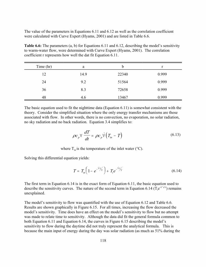
118

(6.13)

(6.14)

The value of the parameters in Equations 6.11 and 6.12 as well as the correlation coefficientwere calculated with Curve Expert (Hyams, 2001) and are listed in Table 6.6.

Table 6.6: The parameters (a, b) for Equations 6.11 and 6.12, describing the model’s sensitivityto warm-water flow, were determined with Curve Expert (Hyams, 2001). The correlationcoefficient r represents how well the dat fit Equation 6.11.

Time (hr) a b r

12 14.9 22340 0.999

24 9.2 51564 0.999

36 8.3 72658 0.999

48 4.6 13467 0.999

The basic equation used to fit the nighttime data (Equation 6.11) is somewhat consistent with thetheory. Consider the simplified situation where the only energy transfer mechanisms are thoseassociated with flow. In other words, there is no convection, no evaporation, no solar radiation,no sky radiation and no back radiation. Equation 3.4 simplifies to:

( )ρ ρcdTdt

c T Tp p in∀ = ∀ −&

where Tin is the temperature of the inlet water (°C).

Solving this differential equation yields:

T T e T ein

t

i

t= −

+−∀ ∀ −∀ ∀1

& &

The first term in Equation 6.14 is in the exact form of Equation 6.11, the basic equation used todescribe the sensitivity curves. The nature of the second term in Equation 6.14 (Tie-œ’ t/œ) remainsunexplained.

The model’s sensitivity to flow was quantified with the use of Equation 6.12 and Table 6.6.Results are shown graphically in Figure 6.15. For all times, increasing the flow decreased themodel’s sensitivity. Time does have an effect on the model’s sensitivity to flow but no attemptwas made to relate time to sensitivity. Although the data did fit the general formula common toboth Equation 6.11 and Equation 6.14, the curves in Figure 6.15 describing the model’ssensitivity to flow during the daytime did not truly represent the analytical formula. This isbecause the main input of energy during the day was solar radiation (as much as 51% during the

119

0

100000

200000

300000

400000

500000

600000

700000

0 10 20 30 40

Flow ( x 10-6 (m3/s)/m3)

Sens

itivi

ty (°

C/(m

3 /s)/m

3 )

12 hours24 hours36 hours48 hours

Figure 6.15: The model’s sensitivity to warm water flow rates decreased exponentially as the flowincreased, illustrating how the sensitivity was dependant on the flow rate.

day), not flow (0% during the day). Therefore, Equation 6.13 is not valid and its solution,Equation 6.14, did not analytically represent the daytime situation.

6.3.5 Variations in Flow - Cool Water (15°C)

Increasing the flow of cool water (15°C) to the pond decreased the pond temperature withrespect to the standard model run (see Figure 6.16). The pond temperature after 48 hours for thestandard was 33.0°C while the temperature of the pond after 48 hours for trial 31 (flow = 3.33 x10-5 m3/s) was 20.0°C, a difference of 13°C.

Depending on the flow rate, the cool water removed the energy gained by the pond during theday from solar radiation. The night time low for trial 31 was 17.1°C on the first night and17.1°C on the second night. The night time low for trial 30 (flow = 2.5 x 10-5 m3/s) was 17.6°Con the first night and 18.2°C on the second night an increase in 0.6°C. This increasedemonstrates that the flow of cold water is barely removing all the solar energy gained duringthe course of the day.

The rate at which the temperature decreased in the ponds during the night was also dependant onthe flow rate. For the first night, the lowest flow regime (trial 26, flow = 2.08 x 10-6 m3/s) caused

120

0

10

20

30

40

0:00 7:59 16:00 0:00 7:59 16:00 0:00

Time

Pond

Tem

pera

ture

(°C

)0

2.14.28.4

16.7 25.0

33.3

Figure 6.16: The pond temperature decreased as the flow of cool 15°C water increased. Thenumbers in the legend are flow readings and have the units 10-6 ((m3/s)/m3). Only one flowrate (flow rate = 33.3 x 10-6 (m3/s)/m3 was able to remove all the solar energy gained by thepond.

-14

-12

-10

-8

-6

-4

-2

0

0 0.00001 0.00002 0.00003 0.00004

Flow (m3/s)/m3

Tem

pera

ture

Diff

eren

ce (°

C)

12 hours24 hours36 hours48 hours

Figure 6.17: Changes in the model’s output when compared with changes in cool water flowincreased absolutely with flow and time. The shape of these associated exponential curvespartially agrees with the theory.

121

the pond to cool at a rate of 0.21°C/hr whereas for the highest flow regime (trial 31), the rate thepond cooled was 0.70°C/hr. The difference between the pond temperature for the trials and thestandard increased as the flow of cold water increased (see Figure 6.17). As time progressed, thetemperature difference between the trials and the standard also increased. Increasing the flowfrom 0 m3/s to 3.33 x 10-5 m3/s increased the temperature difference between the standard and thetrials by 2.3°C after 12 hours and 13.0°C after 48 hours.

Again, the model’s sensitivity to flow was quantified by fitting the data in Figure 6.17 toEquation 6.11, using Curve Expert (Hyams, 2001). Parameters in Equation 6.11 for the coolwater model runs as well as the correlation coefficient are shown in Table 6.7

Table 6.7: Parameters (a, b) used in Equation 6.12 determined the model’s sensitivity to coldwater flow. The correlation coefficient r represents how well the data fits Equation 6.11.

Time (hr) a b r

12 4.4 22285 0.999

24 11.4 30615 0.999

36 10.7 51095 0.999

48 15.4 54781 0.999

The model’s sensitivity to cool water flow (shown in Figure 6.18) decreased as the flow rateincreased. For instance, after 24 hours, the sensitivity dropped from 348 712°C/(m3/s)/m3 to 125682°C/(m3/s)/m3. Changes in sensitivity were greatest at 48 hours (708 805 °C/( m3/s)/m3) andsmallest at 12 hours (51 100°C/(m3/s)/m3). Although this shows that time does have someimpact on the model’s sensitivity to flow, no relationship between time and sensitivity wassought. This is because Equation 6.11, although empirically accurate in fitting the data in Figure6.17, is not the proper simplified solution to Equation 3.4. In other words, the curves describingthe model’s sensitivity to flow during the daytime do not reflect the fact that there was no flowduring the daytime.

6.3.6 - Overall Conclusions from the Sensitivity Analysis

For the aquaculturist, the sensitivity analysis is as an opportunity to determine which factorshave a greater effect in controlling the pond temperature. By comparing the model’s sensitivityto air temperature, solar radiation, wind speed and warm or cool water flow rates, factors whichare important in controlling pond temperature should become obvious. However, there areproblems with direct comparisons of the numerical values for sensitivity:

• Sensitivity was a function of time. Comparisons between the sensitivity for variations oftwo different parameters, for example air temperature and wind speed, could only be done

122

0100000200000300000400000500000600000700000800000900000

0 0.00001 0.00002 0.00003 0.00004

Flow ((m3/s)/m3)

Sens

itivi

ty (°

C/(m

3 /s)/m

3 )

12 hours24 hours36 hours48 hours

Figure 6.18: The model’s sensitivity decreased exponentially as the flow rate of cool waterincreased. Therefore, changing the flow for low flows had a greater impact on the model’ssensitivity. A relationship between the model’s sensitivity to flow and time cannot be foundbecause the 24 hour curve and the 36 hour curve crossed.

forgiven time, since for all trials, as time increased, the sensitivity also increased.

• Sensitivity, in some cases, was a function of the parameter varied. This applied toparameters where the derivative to the general equation used to fit the data in thesensitivity graphs (Figures 6.3, 6.6, 6.10, 6.13, 6.17) were dependant on the variedparameter. For variations in air temperature and solar radiation, a straight line was usedto relate changes in the output to changes in the input. The derivative of a straight line(and therefore, the model’s sensitivity to that particular parameter) was a constant. Therefore, for variations in air temperature and solar radiation, the model’s sensitivitywas not a function of these parameters. However, this was not the case for variations inwind speed and flow rates. For wind speed, the derivative of the general equation used tofit the data in Figure 6.10 (Equation 6.9 is the curve of best fit, Equation 6.10 is Equation6.9's derivative) was still a function of wind speed. Likewise, for variations in flow ratesof warm or cool water, the derivative of Equation 6.11, Equation 6.12, remained afunction of the flow rate. Therefore, when comparing the model’s sensitivity fordifferent variable inputs, certain variables must be held fixed.

• The units for various sensitivity measurements were different. You cannot compareapples to oranges. Similarly, comparisons between sensitivity values with units °C/°C,

123

°C/Wattt, °C/(m/s) or °C/(m3/s)/m3 were not possible because each sensitivity value wasmeasuring something different.

For these reasons, direct quantitative comparisons of sensitivity values were not possible. However, comparisons were possible if absolute variations in input were set at a specific value. For example, no comparison between the model’s sensitivity to air temperature(0.00695°C/°C/hr) and the model’s sensitivity to solar radiation (0.0029°C/Watt/hr) could bemade. However, a comparison could be made between a change in air temperature of +5°C for12 hours (absolute change in output = 0.417°C) and a reduction of 25% of the maximum solarradiation for 12 hours (absolute change in output = -1.078°C). In this case, changing the solarradiation had more of an effect in changing the pond temperature. So, in this case, the model’ssensitivity to changes in solar radiation was greater than the model’s sensitivity to changes in airtemperature.

By doing such comparisons for specific set parameters, it becomes possible to tell whichparameters have a greater effect on the model’s output, especially if those set parameters are setto extreme cases.

Changing the average air temperature did relatively little affecting the pond temperature, whencompared to variations in other input parameters. According to the theory, a change in the airtemperature should directly affect convection because the temperature gradient between the pondand the air increases. Lowering the average air temperature to 0°C after 48 hours (absolutechange in output = 6.3°C) was not as effective as increasing the wind speed from 0 to 10 m/s (or0 to 22.4 mph) (absolute change in output = 9.4°C) or increasing the flow rate of cool 15°Cwater from 0 to 1.67 x 10-5 (m3/s)/m3 (absolute change in output = 9.2°C). Because thesuggested variations in flow or wind speed were much more realistic than the suggestedvariations in air temperature for Baton Rouge, Louisiana, an aquaculturist, from that area, tryingto keep the pond temperature artificially high, should be more concerned about windy nightsrather than a cool nights.

Solar radiation, when left unbalanced, caused large increases in pond temperature. Over 48hours, the difference in pond temperature for the standard model run (100% solar radiation, pondtemperature = 33.0°C) and the trial run with no solar radiation (pond temperature = 18.5°C) was14.5°C. A pond temperature of 18.5°C is more realistic than a pond temperature of 33°C. However, the scenario which made the pond temperature “realistic” was in itself unrealistic. Therefore, two observations can be drawn from this:

• Solar radiation was an important energy vector, since it can theoretically, when leftunchecked, cause the pond temperature to increase by 13°C in 2 days. This increase waseven more pronounced for the trial runs where the flow rate for the warm water (36°C)was varied. In this case, for a flow rate of 3.33 x 10-5 (m3/s)/m3, the pond temperatureincreased by 17.4°C in 48 hours.

124

• Solar radiation, for unheated ponds, had to be balanced, either by one or a combination ofnegative energy vectors. Such energy vectors included evaporation, where increasing thewind speed from 0 to 2 m/s decreased the standard pond temperature by 13.4°C to a pondtemperature of 19.5°C. This underlines the importance of evaporation as a prominentenergy transport mechanism.

The sensitivity analysis, although insightful, failed to determine the model’s sensitivity tointeracting parameters (Saltelli, 2000). This is the main drawback of the “one at a time” type ofsensitivity analysis. For instance, increasing wind speed while decreasing solar radiation wouldhave caused the model’s output to change differently from the standard. Other techniques doexist and are described in detail in Saltelli, Chan and Scott (2000).

6.4 Conclusions

A sensitivity analysis was performed on PHATR Version 1.2. Four parame ters were varied one ata time to determine how sensitive the model’s output was to changes in the input. These fourparameters were 1) average air temperature, 2) solar radiation, 3) wind speed and 4) flow rate ofinlet water. Another goal of the sensitivity analysis was to determine certain counter-intuitivephenomena present under different scenarios.

The sensitivity was described as the derivative of the relationship between the output (y-axis)and the input (x-axis). In this way, the sensitivity was quantified.

For variations in the average air temperature, the pond temperature varied linearly for a fixedtime (slope = derivative = sensitivity = 0.10 °C/°C at 12 hours to 0.35°C/°C at 48 hours). Thesensitivity also varied linearly with time (0.00695 °C/°C/hr).

Similarly, variations in solar radiation caused the pond temperature to vary linearly as well. Inthis case, both the slope and the intercept for each sensitivity curve (line) was calculated. Thesensitivity ranged from 0.041 °C/W (at 12 hours) to 0.154 °C/W (at 48 hours) and varied linearlywith time, according to the equations presented in Figure 6.7

The sensitivity varied linearly with time only because time steps of 12 hours were chosen. Hadany other time step been chose, the sensitivity would not have varied linearly.

Increasing the wind speed increased nighttime evaporation, which caused the ponds to cooldown. This made the pond cooler than the air during the day. In doing so, the air vapor pressurebecame greater than the water vapor pressure (thus preventing evaporation from occurring). Furthermore, the air through convection warmed the pond. This explains why the pondtemperature did not decrease further during the day for increased wind speeds (see Figure 6.9).

The model’s sensitivity to wind speed was calculated by taking the derivative of the equationwhich best fit the sensitivity curves in Figure 6.10. An associated exponential function was used

125

to fit the data in all four cases. The model’s sensitivity was again dependant on time, althoughno relationship between time and the parameters for the associated exponential function wassought.

Increasing the flow rate of warm water to the pond increased the pond temperature andincreasing the flow rate of cool water to the pond decreased the pond temperature. Anexponential association was found to be the curve of best fit between the standard trial pondtemperature difference and the flow rates. An exponential association is very similar to thesimplified theoretical solution of the energy balance equation (Equation 3.4). The model’ssensitivity to flow was calculated by taking the derivative of the exponential association equationand substituting in the statistically determined constants.

By knowing the model’s sensitivity to variations in input, the output error associated with faultyinput data can be estimated using the sensitivity curves and relations presented here. Althoughthe curves cannot directly predict errors in the model output, they can generate an idea of howthe model’s output will change. Furthermore, the sensitivity analysis was an other way ofdetermining which energy transfer mechanisms were important. Because the inherent errors inthe empirical equations used by PHATR cause errors in the output, the sensitivity analysisrevealed how important these errors might be.

126

CHAPTER 7 - USING PHATR FOR DESIGN AND MANAGEMENT APPLICATIONS

7.1 Introduction

PHATR, a computer model which solves 3.4, the differential equation describing the energybalance for a small (volume = 400 m3) well-mixed aquaculture pond (see Chapter 4), wasspecifically designed to determine the pond temperature for the “warm water ponds” at theLouisiana State University (LSU) Aquaculture Research Station (ARS). It was also meant to beused as a design tool for engineers or as a management tool for aquaculturists for the warm waterponds. Because the model still needs to be validated for larger ponds or ponds in differentclimates, PHATR should not be used by engineers or aquaculturists for the following types ofponds:

• ponds located in a climate different from that experienced in Louisiana • ponds which are poorly mixed • ponds which are much larger than 400 m3

• ponds where there is little recorded information about the weather.

However, for the warm water ponds at the Louisiana State University Aquaculture ResearchStation (LSU ARS), PHATR has been validated and was used to answer these design andmanagement questions:

1) What is the pond temperature throughout a year?2) What is the energy surplus or deficit when keeping the pond temperature constant?3) By how much does the temperature decrease in one night if there is suddenly no way to keepthe pond warm?4) What are the flow requirements for increasing the pond temperature by 2°C/day during atypical week in January?

7.2 Materials and Methods

PHATR Version 1.2 was used with these added features:

• The effects of rainfall were included as a bulk movement of energy into the pond (see Chapter 3.5.1 for theoretical explanations). • For a given pond temperature (given in a ASCII file), PHATR could calculate the amount of cold and warm water needed to maintain the pond a that temperature. The user specified the temperature of the cold and warm water sources at the user prompt.

Weather data were compiled and generated to produce three weather input files, one for a coldyear, one for an average year and one for a hot year. All the data used to create the weather files,with the exception of solar radiation, were supplied by the Southern Regional Climate Center atLSU.

127

The air temperature, relative humidity and wind speed data used in each file were compiled fromweather data collected between 1952 and 1992 in Baton Rouge every hour, except between 1965to 1972, where the data were collected every 3 hours. No wind speed data were collected priorto 1964. Using a FORTRAN program called “Weather_Generator(a)” (code in Appendix 13),the data were sorted to determine the following weather statistics:

• the maximum temperature of every hour of the year • the minimum temperature of every hour of the year • the average temperature of every hour of the year • the average relative humidity of every hour of the year • the average wind speed of every hour of the year

The normal rainfall data for every day of the year were converted into average hourly rainfallrates. For instance, if 24 cm of rain fell in a day, it was assumed that 1 cm of rain fell every hourduring that day.

Because no solar radiation data for every hour of the year was available, the extra-terrestrialsolar radiation was calculated depending on the pond’s geographic location, the time of day andthe time of year (Appendix 14). A “cloud” factor was multiplied by the solar radiation data tosimulate the absorption of solar radiation by the atmosphere. The cloud factor was equal to 0.85for a hot year and 0.25 for a cold year. For the average year weather data file, the averagepercentage of total solar radiation for a particular month was used as the cloud factor. Theaverage percentage of total solar radiation was available through the Southern Regional ClimateCenter web site (http://www.srcc.lsu.edu/6190/ccd.html).

The “average year” data set consisted of :

• the average temperature of every hour of the year • the average relative humidity of every hour of the year • the average wind speed of every hour of the year • the solar radiation for the average year • the normal rainfall

The “cold year” data set consisted of:

• the minimum temperature of every hour of the year • the average relative humidity of every hour of the year • a constant wind speed of 10 m/s • the calculated solar radiation with a cloud factor of 0.25 • the normal rainfall

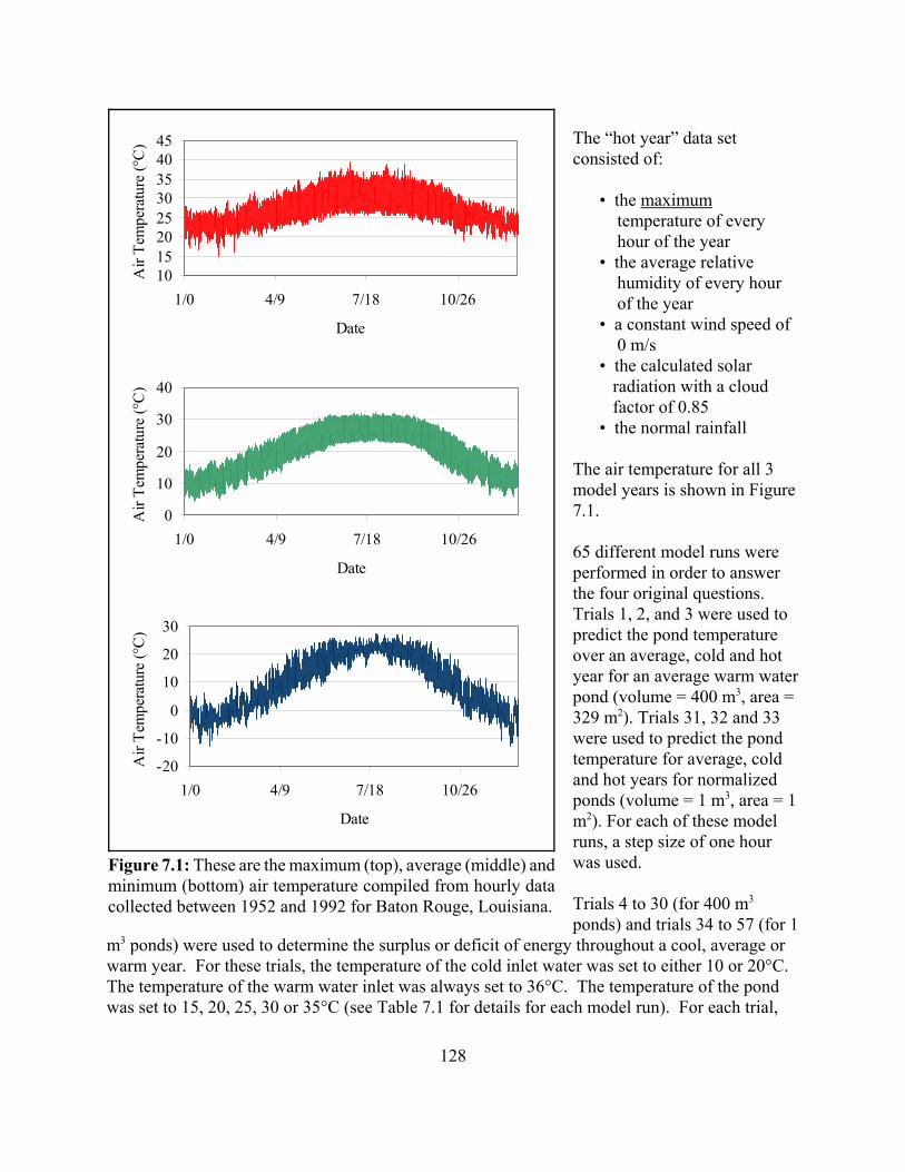
128

1015202530354045

1/0 4/9 7/18 10/26

Date

Air

Tem

pera

ture

(°C

)

0

10

20

30

40

1/0 4/9 7/18 10/26

Date

Air

Tem

pera

ture

(°C

)

-20

-10

0

10

20

30

1/0 4/9 7/18 10/26

Date

Air

Tem

pera

ture

(°C

)

Figure 7.1: These are the maximum (top), average (middle) andminimum (bottom) air temperature compiled from hourly datacollected between 1952 and 1992 for Baton Rouge, Louisiana.

The “hot year” data setconsisted of:

• the maximum temperature of every hour of the year • the average relative humidity of every hour of the year • a constant wind speed of 0 m/s • the calculated solar radiation with a cloud factor of 0.85 • the normal rainfall

The air temperature for all 3model years is shown in Figure7.1.

65 different model runs wereperformed in order to answerthe four original questions. Trials 1, 2, and 3 were used topredict the pond temperatureover an average, cold and hotyear for an average warm waterpond (volume = 400 m3, area =329 m2). Trials 31, 32 and 33were used to predict the pondtemperature for average, coldand hot years for normalizedponds (volume = 1 m3, area = 1m2). For each of these modelruns, a step size of one hourwas used.

Trials 4 to 30 (for 400 m3

ponds) and trials 34 to 57 (for 1m3 ponds) were used to determine the surplus or deficit of energy throughout a cool, average orwarm year. For these trials, the temperature of the cold inlet water was set to either 10 or 20°C. The temperature of the warm water inlet was always set to 36°C. The temperature of the pondwas set to 15, 20, 25, 30 or 35°C (see Table 7.1 for details for each model run). For each trial,

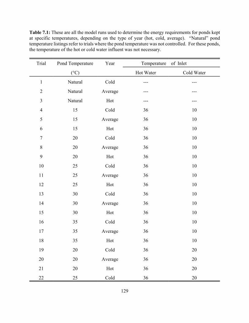
129

Table 7.1: These are all the model runs used to determine the energy requirements for ponds keptat specific temperatures, depending on the type of year (hot, cold, average). “Natural” pondtemperature listings refer to trials where the pond temperature was not controlled. For these ponds,the temperature of the hot or cold water influent was not necessary.

Trial Pond Temperature Year Temperature of Inlet

(°C) Hot Water Cold Water

1 Natural Cold --- ---

2 Natural Average --- ---

3 Natural Hot --- ---

4 15 Cold 36 10

5 15 Average 36 10

6 15 Hot 36 10

7 20 Cold 36 10

8 20 Average 36 10

9 20 Hot 36 10

10 25 Cold 36 10

11 25 Average 36 10

12 25 Hot 36 10

13 30 Cold 36 10

14 30 Average 36 10

15 30 Hot 36 10

16 35 Cold 36 10

17 35 Average 36 10

18 35 Hot 36 10

19 20 Cold 36 20

20 20 Average 36 20

21 20 Hot 36 20

22 25 Cold 36 20

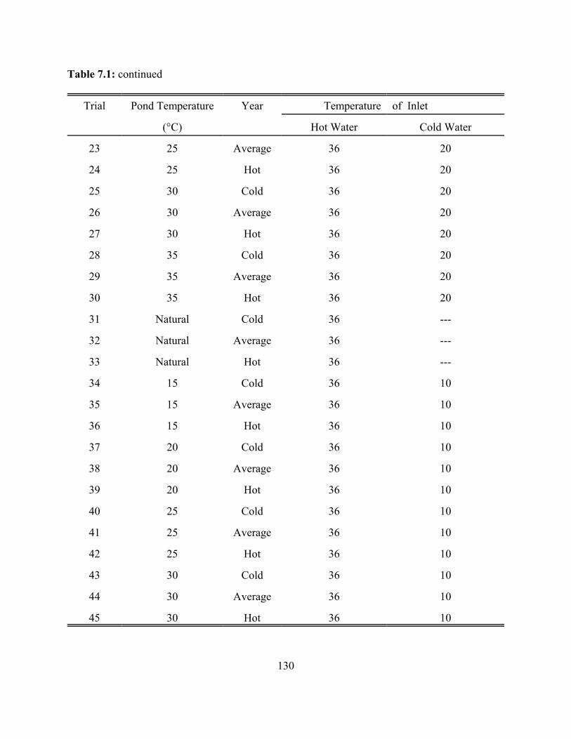
130

Table 7.1: continued

Trial Pond Temperature Year Temperature of Inlet

(°C) Hot Water Cold Water

23 25 Average 36 20

24 25 Hot 36 20

25 30 Cold 36 20

26 30 Average 36 20

27 30 Hot 36 20

28 35 Cold 36 20

29 35 Average 36 20

30 35 Hot 36 20

31 Natural Cold 36 ---

32 Natural Average 36 ---

33 Natural Hot 36 ---

34 15 Cold 36 10

35 15 Average 36 10

36 15 Hot 36 10

37 20 Cold 36 10

38 20 Average 36 10

39 20 Hot 36 10

40 25 Cold 36 10

41 25 Average 36 10

42 25 Hot 36 10

43 30 Cold 36 10

44 30 Average 36 10

45 30 Hot 36 10

131

Table 7.1: continued

Trial Pond Temperature Year Temperature of Inlet

(°C) Hot Water Cold Water

46 35 Cold 36 10

47 35 Average 36 10

48 35 Hot 36 10

49 25 Cold 36 20

50 25 Average 36 20

51 25 Hot 36 20

52 30 Cold 36 20

53 30 Average 36 20

54 30 Hot 36 20

55 35 Cold 36 20

56 35 Average 36 20

57 35 Hot 36 20

the energy surplus or deficit was calculated for every hour of the year. By knowing the energysurplus or deficit, the amount of cold or warm water needed to maintain the pond temperatureconstant was calculated. Trial 58 was used to find out how much warm geothermal well waterwould be needed on a cold January night to keep a 400 m3 pond at 27°C. Trial 59 was used todetermine how quickly a 400 m3 pond, initially at 27°C, cools down during a cold night. Trials58 and 59 used weather data collected during the night of the 23rd to the 24th of January, 2003, atthe Ben Hur weather station. The night time low that night was -6.3°C. The air temperatureprofile, the relative humidity and the wind speed for the time period considered are shown inFigure 7.2. No rainfall was recorded during this time. Both model runs were done for the timeperiod between 17:50, 01/23 (sunset), and 24:00, 01/24. The time step for both runs was 10minutes.

Trials 61, 62, 63 and 64 were used to determined the change in pond temperature for the night ofthe 10th of March, 2003, under different scenarios. (That night was special because thegeothermal well was only turned on at 1:00 AM on the 11th of March.) The weather conditionsfor that night were measured at the Ben Hur Weather Station and are presented in Figure 7.3. The trial ran for the time period 18:22, 03/10 (sunset), and 6:10, 3/11 (sunrise). The time stepwas 10 minutes. The initial pond temperature was measured at 28°C. Trial 61 made use of the

132

-8

-4

0

4

8

17:45 22:33 3:21 8:09 12:57 17:45 22:33

Time

Air

Tem

pera

ture

(°C

)

0

30

60

90 Relative H

umidity (%

)

012345678

17:45 22:33 3:21 8:09 12:57 17:45 22:33

Time

Win

d Sp

eed

(m/s)

.

Figure 7.2: The air temperature, the relative humidity and the wind speed are shown from 17:45on 01/23/03 to 24:00 on 01/24/03. The data, recorded at the Ben Hur Weather Station, representweather conditions were evaporation, convection and longwave pond radiation are important.

unmodified collected weather data. Trial 62 assumed a constant wind speed of 10 m/s after 1:00,3/11. Trial 63 assumed a constant relative humidity of 30% after 1:00, 3/11. Trial 64 assumed aconstant wind speed of 10 m/s and a constant relative humidity of 30% after 1:00, 3/11. Thepond temperature throughout the night was compared to the measured temperature in pond 12. The temperature was measured 10 cm below the surface using a type T thermocouple connectedto a data logger (Campbell Scientific 21X, Campbell Scientific Inc., North Logan, UT). Thetemperature was recorded every 10 minutes. Despite the well being turned on at 1:00, 3/11, the

133

0

5

10

15

20

25

18:28 20:52 23:16 1:40 4:04

Time

Tem

pera

ture

(°C

)

0

25

50

75

100 Relative H

umidity (%

)

0

0.5

1

1.5

2

2.5

18:28 20:52 23:16 1:40 4:04

Time

Win

d Sp

eed

(m/s)

Figure 7.3: The air temperature, the relative humidity and the wind speed recorded at the BenHur Weather Station between 18:28, 03/10/2003 and 6:10, 03/11/2003. These data were usedby PHATR to determine the pond temperature under different scenarios for that night.

model assumed that no water was added to the pond. This was done to see what would havehappened if the well had remained off.

Trial 65 was done to determine the required flow rate needed to gradually increase the pondtemperature from 10.5°C (the modeled pond temperature for January 15th at sundown, using theaverage year weather data file) to 27°C, the temperature maintained at the LSU ARS to

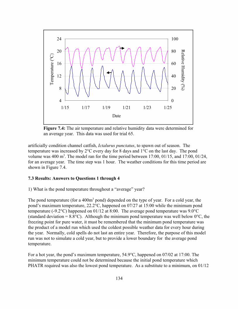
134

4

8

12

16

20

24

1/15 1/17 1/19 1/21 1/23 1/25

Date

Tem

pera

ture

(°C

)

0

20

40

60

80

100

Relative H

umidity (%

)

Figure 7.4: The air temperature and relative humidity data were determined foran average year. This data was used for trial 65.

artificially condition channel catfish, Ictalurus punctatus, to spawn out of season. Thetemperature was increased by 2°C every day for 8 days and 1°C on the last day. The pondvolume was 400 m3. The model ran for the time period between 17:00, 01/15, and 17:00, 01/24,for an average year. The time step was 1 hour. The weather conditions for this time period areshown in Figure 7.4.

7.3 Results: Answers to Questions 1 through 4

1) What is the pond temperature throughout a “average” year?

The pond temperature (for a 400m3 pond) depended on the type of year. For a cold year, thepond’s maximum temperature, 22.2°C, happened on 07/27 at 15:00 while the minimum pondtemperature (-9.2°C) happened on 01/12 at 8:00. The average pond temperature was 9.0°C(standard deviation = 8.8°C). Although the minimum pond temperature was well below 0°C, thefreezing point for pure water, it must be remembered that the minimum pond temperature wasthe product of a model run which used the coldest possible weather data for every hour duringthe year. Normally, cold spells do not last an entire year. Therefore, the purpose of this modelrun was not to simulate a cold year, but to provide a lower boundary for the average pondtemperature.

For a hot year, the pond’s maximum temperature, 54.9°C, happened on 07/02 at 17:00. Theminimum temperature could not be determined because the initial pond temperature whichPHATR required was also the lowest pond temperature. As a substitute to a minimum, on 01/12

135

-20-10

0102030405060

1/0 3/13 5/25 8/6 10/18 12/30

Date

Pond

Tem

pera

ture

(°C

) . (a)

(b)

(c)

Figure 7.5: Modled pond temperature profiles for hypothetical hot (a), cold (b) andaverage (c) years are shown. The hot and cold years are not realistic (note the belowfreezing temperatures for the (c)) but they do bound the possible values for theaverage year.

at 8:00, the pond temperature was 30.0°C. The average pond temperature was 44.1°C (standarddeviation = 7.9°C). Again, a pond temperature of 54.9°C is unlikely to happen in Baton Rouge,Louisiana. However, the purpose of the hot weather model run, not unlike the cold weathermodel run, was to provide an upper boundary for the average pond temperature.

For an average year, the pond’s maximum temperature, 31.7°C, happened on 06/26 at 17:00. The minimum pond temperature, 8.5°C, happened on 01/13 at 8:00. The average pondtemperature was 21.8°C (standard deviation = 7.0°C). The pond temperature for a cold, hot andaverage year are shown in Figure 7.5 Because the model has not yet been validated for summersor early autumn in Baton Rouge, the values generated for this time of year should be consideredwith caution.

2) What is the energy surplus or energy deficit when keeping the pond temperature constant?

Energy demands are dependant on the weather. A cold year was shown to have greater energydemands for keeping the pond warm. For instance, to maintain the pond temperature at 15°C foran entire year, the total energy deficit was 1.18 x 1011 J/m3 (3 284 kWhr/m3). To maintain thepond temperature at 35°C during the same year, the total energy deficit was 7.56 x 1011 J/m3 (21000 kWhr/m3). A hot year, on the other hand, always had a yearly surplus of energy. Tomaintain the pond temperature at 35°C, 4.9 x 109 J/m3 (1371 kWhr/m3) net had to be removed.

136

-2000000

0

2000000

4000000

6000000

1/0 3/15 5/29 8/12 10/26

Date

Ener

gy S

urpl

us/D

efic

it (W

atts)

-4000000

-2000000

0

2000000

4000000

1/0 3/15 5/29 8/12 10/26

Date

Ener

gy S

urpl

us/D

efic

it (W

atts)

-6000000

-4000000

-2000000

0

2000000

1/0 3/15 5/29 8/12 10/26

Date

Ener

gy S

urpl

us/D

efic

it (W

atts)

Figure 7.6: Surpluses and deficits of energy varied over the course of a day and a year.These plots show the energy requirements for a 1 m3 pond over an average weather year.The pond temperature was maintained at 15°C (a), 25°C (b) and 35°C (c). Not shown areplots for 20 and 30°C.

To maintain the pond temperature at 15°C, 1.2 x 109 J/m3 (3295 kWhr/m3) net had to be removed

(see Table 7.2 for more details on energy requirements for maintaining pond temperature).

137

From a design perspective, the energy requirements for an average year were more interestingbecause the model results were more realistic. Maintaining the pond temperature between 20°Cand 25°C during an average year required no additional energy, assuming the pond energysurpluses could be stored for use when the pond had an energy deficit. The total net energysurplus when maintaining the pond temperature at 15°C during an entire average year was 6.9 x109 J/m3 (1919 kWhr/m3). The total net energy deficit when maintaining the pond temperature at35°C during an entire average year was 1.9 x 1010 J/m3 (5175 kWhr/m3). These numbers do notreflect, however, how the pond energy surpluses or deficits changed throughout an average year(see Figure 7.6 for variations in pond energy surpluses/deficits throughout an average year).

Table 7.2: The total energy surpluses and deficits associated with maintaining a 1 m3 pond at agiven temperature are such that the total energy surpluses are positive quantities while the totaldeficits are negative quantities. These values do not reflect how the energy surplus or deficit canchange over a day or year.

Pond Temperature Total Surplus/Deficit (J/m3)

(°C) Cold Year Average Year Hot Year

15 -1.18 x 1010 6.91 x 109 1.19 x 1010

20 -2.38 x 1010 2.52 x 109 1.05 x 1010

25 -3.96 x 1010 -3.24 x 109 8.90 x 109

30 -5.76 x 1010 -1.03 x 1010 7.03 x 109

35 -7.56 x 1010 -1.86 x 1010 4.9 x 109

Table 7.3: Here are estimates for the energy costs associated with maintaining the pond temperatureat a set value for an average weather year. Holding the pond at 20°C was the most inexpensive pondtemperature.

Pond Temperature Energy Costs ($/m3)

(°C) 2¢/kWhr 7¢/kWhr 15¢/kWhr

15 56 195 418

20 54 188 403

25 61 214 460

30 80 281 602

35 111 388 831

138

The cost associated with heating or cooling a 1 m3 pond was calculated every hour for anaverage year. The cost of heating or cooling one kilowatt-hour was assumed to be the same. The unit cost for electricity was assumed to be either $0.02/kWh, $0.07/kWh or $0.15/kWh. (Based on 2003 rates, the cost for electricity for large-scale commercial operations in BatonRouge, Louisiana, is $0.0317 for the first 50 kWh, $0.0297 for the next 100 kWh, $0.02776 forthe following 225 kWh and $0.02576 kWh for any additional energy requirements.) The totalcost to maintain the pond temperature constant during an average year is presented in Table 7.3.Keeping a pond at 20°C proved to be the least expensive ($54/m3). This is not surprising sincethe average temperature of an unheated pond during an average year was 21.8°C.

If geothermally enriched warm water is used to control the pond temperature, the maximum andaverage flow rates, used for choosing a pump, were calculated. These values are dependant onthe temperature of the incoming water. For the trials used here, the “warm” water was set to36°C while the “cool” water was set to either 10°C and 20°C. Maximum and average flow ratesfor an average year for each temperature setting are presented in Table 7.4. The required flowrates were smaller if the difference between the inlet water temperature and the pond temperaturewas small. For instance, an average flow rate of 1.99 x 10-6 (m3/s)/m3 (0.032 gpm/m3) was required when using 10°C water to maintain the pond temperature at 25°C during an averageyear. When using 20°C water, the required average flow rate was 5.97 x 10-6 (m3/s)/m3 (0.095gpm/m3) - 3 times as much water. There are other reasons why it is desirable to increase thedifference between the pond and inlet water temperature for the purposes of pond temperaturecontrol:

• to reduce the sizing of pumps. For keeping the pond temperature at 25°C using20°C water, 3 times as much water was needed on average than if the inlet watertemperature was 10°C. The peak required flow rates were also greater whenusing 20°C water (4 x 10-5 (m3/s)/m3 as opposed to using 10°C inlet water (1.3 x10-5 (m3/s)/m3 ).

• to reduce the amount of wasted water. By adding water into a pond, assuming thepond volume was kept constant, water must be displaced out of the pond. Thewater was not re-used, wasted and may be considered a loss to the farm.

• to reduce pumping costs. By reducing the amount of water needed, the costsassociated with pumping could also be reduced.

3) By how much does the temperature decrease in one night if there is suddenly no way to keepthe pond warm?

For the night of the 23rd to the 24th of January, 2003, the average air temperature was -3.1°C andthe lowest pond temperature was -6.3°C. If the pond temperature, at sunset, was 27°C, then bysunrise, the pond temperature was 19.2°C. By sunset on the 24th of January, the pondtemperature had gone down to 18.1°C and by 24:00, the pond temperature was 16.8°C (seeFigure 7.7). There are several reasons for the large decline in pond temperature. Because the

139

Table 7.4: These were the flow requirements for 10°C, 20°C and 36°C water to maintain constantpond temperature during an average weather year (pond size = 1m3). The standard deviation (St.Dev.) was an indicator of how the average flow rate varied over the course of a year. For designpurposes, both the maximum and the average flow rate were required. The 10°C and the 20°Cwater were used to cool the ponds. The 36°C water was used to warm up the ponds.

Inlet water temperature = 10°C

Tpond Maximum Flow Average Flow St. Dev.

(°C) ((m3/s)/m3) (gpm/m3) ((m3/s)/m3) (gpm/m3) ((m3/s)/m3)

15 5.20 x 10-5 8.25 x 10-1 1.30 x 10-5 2.06 x 10-1 1.55 x 10-5

20 2.40 x 10-5 3.81 x 10-1 4.67 x 10-6 7.41 x 10-2 6.98 x 10-6

25 1.30 x 10-5 2.06 x 10 -1 1.99 x 10-6 3.16 x 10-2 3.71 x 10-6

30 7.00 x 10-6 1.11 x 10-1 7.86 x 10-7 1.25 x 10-2 1.80 x 10-6

35 3.00 x 10-6 4.76 x 10-2 2.01 x 10-7 3.19 x 10-3 6.48 x 10-7

Inlet water temperature = 20°C

Tpond Maximum Flow Average Flow St. Dev.

(°C) ((m3/s)/m3) (gpm/m3) ((m3/s)/m3) (gpm/m3) ((m3/s)/m3)

15 --- --- --- --- ---

20 --- --- --- --- ---

25 4.00 x 10-5 6.35 x 10-1 5.97 x 10-6 9.48 x 10-2 1.11 x 10-5

30 1.50 x 10-5 2.38 x 10-1 1.58 x 10-6 2.51 x 10-2 3.59 x 10-6

35 6.00 x 10-6 9.52 x 10-2 3.36 x 10-7 5.33 x 10-3 1.06 x 10-6

Inlet water temperature = 36°C

Tpond Maximum Flow Average Flow St. Dev.

(°C) ((m3/s)/m3) (gpm/m3) ((m3/s)/m3) (gpm/m3) ((m3/s)/m3)

15 4.00 x 10-6 6.35 x 10-2 5.66 x 10-7 8.98 x 10-3 1.03 x 10-6

20 8.00 x 10-6 1.27 x 10-1 1.71 x 10-6 2.71 x 10-2 2.35 x 10-6

25 1.60 x 10-5 2.54 x 10-1 4.97 x 10-6 7.89 x 10-2 4.91 x 10-6

30 3.80 x 10-5 6.03 x 10-1 1.46 x 10-4 2.31 1.19 x 10-5

35 2.94 x 10-4 4.67 51.48x 10-4 2.35 8.67 x 10-5

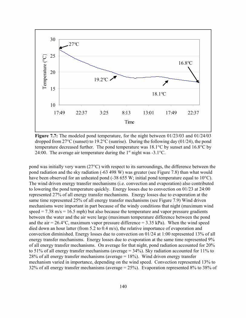
140

10

15

20

25

30

17:49 22:37 3:25 8:13 13:01 17:49 22:37

Time

Tem

pera

ture

(°C

)27°C

19.2°C

18.1°C

16.8°C

Figure 7.7: The modeled pond temperature, for the night between 01/23/03 and 01/24/03dropped from 27°C (sunset) to 19.2°C (sunrise). During the following day (01/24), the pondtemperature decreased further. The pond temperature was 18.1°C by sunset and 16.8°C by24:00. The average air temperature during the 1st night was -3.1°C.

pond was initially very warm (27°C) with respect to its surroundings, the difference between thepond radiation and the sky radiation (-63 498 W) was greater (see Figure 7.8) than what wouldhave been observed for an unheated pond (-38 655 W; initial pond temperature equal to 10°C). The wind driven energy transfer mechanisms (i.e. convection and evaporation) also contributedto lowering the pond temperature quickly. Energy losses due to convection on 01/23 at 24:00represented 27% of all energy transfer mechanisms. Energy losses due to evaporation at thesame time represented 25% of all energy transfer mechanisms (see Figure 7.9) Wind drivenmechanisms were important in part because of the windy conditions that night (maximum windspeed = 7.38 m/s = 16.5 mph) but also because the temperature and vapor pressure gradientsbetween the water and the air were large (maximum temperature difference between the pondand the air = 26.4°C, maximum vapor pressure difference = 3.35 kPa). When the wind speeddied down an hour latter (from 5.2 to 0.4 m/s), the relative importance of evaporation andconvection diminished. Energy losses due to convection on 01/24 at 1:00 represented 13% of allenergy transfer mechanisms. Energy losses due to evaporation at the same time represented 9%of all energy transfer mechanisms. On average for that night, pond radiation accounted for 20%to 51% of all energy transfer mechanisms (average = 34%). Sky radiation accounted for 11% to28% of all energy transfer mechanisms (average = 18%). Wind driven energy transfermechanism varied in importance, depending on the wind speed. Convection represented 13% to32% of all energy transfer mechanisms (average = 25%). Evaporation represented 8% to 38% of

141

-80000

-60000

-40000

-20000

0

17:45 20:09 22:33 0:57 3:21 5:45

Time

Diff

eren

ce B

etw

een

Pond

and

Lon

gwav

Sky

Rad

iatio

n (W

atts

)

Unheated Pond

Heated Pond

Figure 7.8: Each line represents the difference between longwave pond radiation and longwave skyradiation for a heated or unheated pond. The heated pond, maintained at 27°C, was assumed to loseits source of warm 36°C water at 17:45 (sunset) on 01/23/03, at which point, the pond coolednaturally. The unheated pond model run had an initial pond temperature of 10°C. Because theheated pond was warmer, it radiated and lost more heat than the unheated pond. The averagetemperature for the night was -3.1°C.

all energy transfer mechanisms (average = 23%). The amount of 36°C water required to keep a400 m3 pond at 27°C from sunset on 01/23 to 24:00 on 01/24, ranged from 0 to 15.1 x 10-3 m3/s(0 to 240 gpm) with an average flow rate of 5.90 x 10-3 m3/s (0 to 94 gpm) (see Figure 7.10 forflow demands for the model run).

For a warmer night (3/10 to 3/11, 2003, average air temperature = 14.9°C), changes in pondtemperature were not as drastic. Between 18:22, 03/10 and 6:00, 03/11, the pond temperaturedecreased by 2.0°C. If the wind speed was 10 m/s as opposed to 0.6 m/s, the average wind speedfor that night, the decrease in pond temperature would have been 5.1°C. If the relative humidityhad been 30% as opposed to 82%, the average relative humidity for that night, the decrease inpond temperature would have been 2.2°C. If both the relative humidity and the wind speed werechanged (relative humidity = 30% instead of 82% and wind speed = 10 m/s instead of 0.6 m/s),the change in pond temperature would have been 6.0°C.

142

-100%

-80%

-60%

-40%

-20%

0%

20%

40%

24:00 1:00

Rel

aviti

ve Im

porta

nce

ConvectionEvaporationSky RadiationPond Radiation

Figure 7.9: At 24:00 on 01/23/2003, the wind speed was 3.65 m/s. At this time, wind drivenenergy transfer mechanisms (convection: 27%, evaporation: 25%) were as importance as longwave radiation mechanisms (pond radiation: 31%, sky radiation: 17%). One hour later, at1:00, the wind speed was 0.5 m/s. As a result, convection (13%) and evaporation (9%) werenot as important as pond radiation (51%) or sky radiation (27%). The energy balance wasperformed for a 400 m3 pond.

0

0.004

0.008

0.012

0.016

17:45 22:33 3:21 8:09 12:57 17:45 22:33

Time

Flow

Rat

e (m

3/s)

.

0

100

200

300 Flow R

ate (GPM

) .

Figure 7.10: Between 17:45, 01/23/03 and 24:00, 01/24/03, the flow rate of 36°C water neededto maintain a pond temperature of 27°C was estimated. The flow rates varied between 0 and15.1 x 10-3 m3/s (0 to 240 gpm) with an average flow rate of 5.90 x 10-3 m3/s (94 gpm). Thepond was 400 m3. The average night time temperature during the first night was -3.1°C.

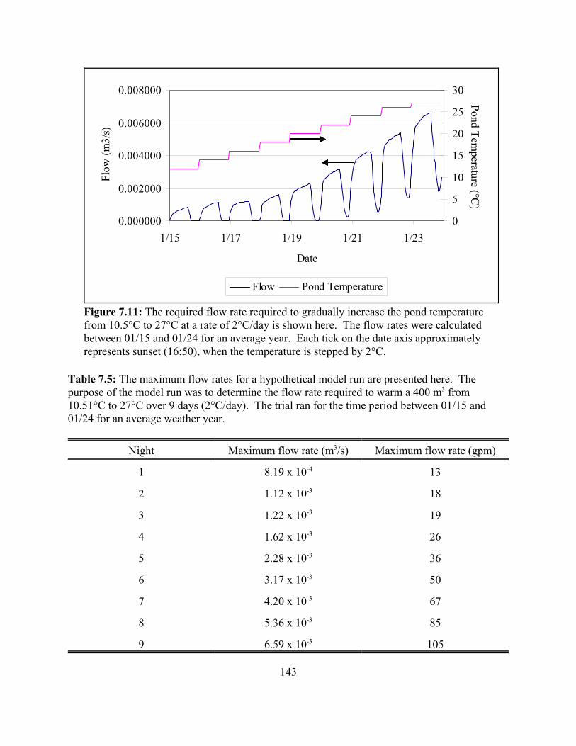
143

0.000000

0.002000

0.004000

0.006000

0.008000

1/15 1/17 1/19 1/21 1/23

Date

Flow

(m3/

s)

0

5

10

15

20

25

30Pond Tem

perature (°C)

Flow Pond Temperature

Figure 7.11: The required flow rate required to gradually increase the pond temperaturefrom 10.5°C to 27°C at a rate of 2°C/day is shown here. The flow rates were calculatedbetween 01/15 and 01/24 for an average year. Each tick on the date axis approximatelyrepresents sunset (16:50), when the temperature is stepped by 2°C.

Table 7.5: The maximum flow rates for a hypothetical model run are presented here. Thepurpose of the model run was to determine the flow rate required to warm a 400 m3 from10.51°C to 27°C over 9 days (2°C/day). The trial ran for the time period between 01/15 and01/24 for an average weather year.

Night Maximum flow rate (m3/s) Maximum flow rate (gpm)

1 8.19 x 10-4 13

2 1.12 x 10-3 18

3 1.22 x 10-3 19

4 1.62 x 10-3 26

5 2.28 x 10-3 36

6 3.17 x 10-3 50

7 4.20 x 10-3 67

8 5.36 x 10-3 85

9 6.59 x 10-3 105

144

PHATR has a tendency of over-predicting the pond temperature so actual decreases in pondtemperature were most likely greater than what was calculated here.

4) What are the flow requirements for increasing the pond temperature by 2°C/day during atypical week in January?

Because January is the coldest month of the year, warming the ponds to induce channel catfishspawning at this time of year represented the worst case scenario. For a 400 m3 pond, with aninitial pond temperature of 10.51°C, the required flow rate of 36°C water for each night isgraphically shown in Figure 7.11. Each night, the peak flow rate increased as shown in Table7.5, with the maximum flow rate happening on the last night before sunrise (6.59 x 10-3 m3/s =105 gpm). No warm water was needed during the daytime until the 5th day (01/20). Themaximum flow rate required during noon, 2.04 x 10-3 m3/s , occurred on the 01/24. The totalenergy required to warm the pond over this time period was 7.64 x 1010 J (21 236 kWh).

7.4 Conclusions

The model answered four design and management questions for the warm water ponds at theLSU ARS. These results should not be seen as an exact answer but rather as an approximationof what could happen. Because Fisfhfry has a tendency of over-predicting the pondtemperature, reported calculated energy deficits are smaller than those in reality and reportedcalculated energy surpluses were larger than those in reality. Furthermore, using the resultspresented in this chapter for ponds other than the LSU ARS warm water ponds should be donewith great caution. In addition to assuming the ponds were well mixed, PHATR was validatedonly for research-sized ponds (400 m3) in a temperate humid climate during the late fall, winterand spring. Using the model despite these warnings is left to the user’s own risk.

The temperature for an unheated pond during cold, hot and average years were estimated. Results from the cold and hot years were seen as boundaries for possible pond temperatures andnot as a pond temperature profile during an extreme case year. The average pond temperature foran average year was 21.8°C with a maximum temperature of 31.7°C and a minimum temperatureof 8.5°C.

The net energy needed to maintain the pond temperature at 15, 20, 25, 30 and 35°C wascalculated for a cold, hot and average year. For an average year, maintaining the pondtemperature between 20 and 25°C required less energy. This is understandable since the averagepond temperature for an average year for an unheated pond, 21.8°C, was between 20 and 25°C.

Temperature decreases for heated ponds in one night were dependant on the specific weatherconditions. For instance, on a cold night, where the average night time temperature was -3.1°Cand the maximum wind speed was 7.4 m/s, the modeled pond temperature decreased from 27°Cto 19.2°C in one night. This was in part because of the unbalanced loss of energy throughlongwave pond radiation. Because the pond’s surroundings were at least 20°C cooler than that

145

of the surroundings, back radiation was much greater than sky radiation, causing the pond toloose energy. Pond radiation accounted for 20% to 51% of all energy transfer mechanisms(average = 34%). Wind driven energy transfer mechanism varied in importance, depending onthe wind speed. Convection represented 13% to 32% of all energy transfer mechanisms (average= 25%). Evaporation represented 8% to 38% of all energy transfer mechanisms (average =23%). On a warmer night (average temperature = 14.9°C), the modeled pond temperaturedecreased from 27°C to 25°C. This is because there was little wind that night and thetemperature difference between the pond and the surroundings was smaller than during the coldnight.

The amount of energy needed to raise the pond temperature (volume = 400 m3) from 10.5°C to27°C at a rate of 2°C/day was modeled to be 7.64 x 1010 J over 9 days.. The required flow rate ofwarm 36°C water was calculated. On the final night, the maximum required flow rate was 2.04x 10-3 m3.

Because the model has proven itself as a good design and management tool, it could be used toaddress other questions about the warm water ponds. By validating PHATR for other situations,the model’s applicability would become more universal.

146

(8.1)

CHAPTER 8: CONCLUSIONS

An energy balance model, called PHATR (Pond Heating And Temperature Regulation), wascreated, tested and validated based on the temperature in 400-m3 earthen aquaculture ponds,given information about the weather, pond characteristics and the flow rate of warm waterentering the pond. The model estimated energy surpluses and deficits which needed to bebalanced to control the pond temperature. Mathematically, PHATR is a computer programwhich solves the following differential equation:

dEdt

q q q q q q q q q q qpond

solar back sky evap conv cond seep rain well out other

= − + − ± ± − + + − ±

where E is the total energy at any given time (t) in the pond qsolar is the rate of energy gained by the pond through solar radiationqback is the rate of heat lost through back radiation qback is the rate of heat gained by longwave sky radiation qsoil is the rate of heat exchanged with the soilqconv is the rate of heat exchanged with the air by convection qevap is the rate of heat lost through the evaporation of water qrain is the rate of bulk energy gained due to rainfall qwell is the rate of bulk energy gained from the warm water well qout is the rate of bulk energy lost to the overflow of waterqother is the rate of energy transfer from or to other sources.

Equation 8.1 is a mathematical representation of the conceptual model presented in Figure 3.1and again in Figure 4.1.

Model runs showed that for unheated ponds, the transport of energy through radiation dominatedall energy transfer mechanisms. Solar radiation was found to account for as much as 55% of allenergy transferred. Longwave pond radiation and longwave sky radiation accounted for no lessthan 19% and 14% respectively of all energy transfer mechanisms during the trial runs. Wind-driven energy transport mechanisms were on average less important (average importance ofconvection was 5%, average importance of evaporation was 6%). Although heat exchangedthrough the soil was equal in average importance to evaporation (2 to 6%), its importance neverexceeded 13%. Because of this, and because including soil heat transfer mechanisms hinderedthe model’s ability to estimate pond temperatures, subsequent model runs did not include theeffects of soil heat transfer (see Chapter 4 for more details).

Model runs also showed that for heated ponds, the bulk transport of energy from warm wellwater accounted for as much as 60% of all energy transport mechanisms. However, at the sametime, energy lost in the discharged water was also substantial (maximum importance was 44%). During the day, solar radiation could account for as much as 50% of all energy transport

147

Influent 19%

PondEffluent

15%

Back Radiation 25%

Longwave sky Radiation 19%

Cloud

Soil 1%

Evaporation 10%

Convection 6%

Solar Radiation 7%

Influent 19%

PondEffluent

15%

Back Radiation 25%

Longwave sky Radiation 19%

Cloud

Soil 1%

Evaporation 10%

Convection 6%

Solar Radiation 7%

Figure 8.1: These results for the energy balance (Chapter 4) illustrate the relative averageimportance for each energy vector for heated ponds. This particular energy balance was developedusing data from the spring of 2003.

phenomena. The average importance of longwave pond radiation was 25% and of longwave skyradiation was 19%. Heat transferred through the soil was not as important (average importance= 1%) (see Chapter 4 for more details).

PHATR had a tendency to over-estimate when predicting pond temperatures (average bias forunheated ponds was 0.5°C; average bias for heated ponds was 2.6°C). Efforts should be made tobetter understand evaporation and convection in future studies. Because both of these transportphenomena were determined empirically, and because both were governed by similar transportprocesses, understanding how the water and air boundary layers behave would be beneficial. The current version of PHATR assumes that the water is a static solid when in reality, heat musttravel through a water and air boundary layer. Further study of the effects of these boundaries todevelop better predictive equations are required.

The absorption of solar radiation in aquaculture ponds also needs to be studied further. Thisstudy did not quantify how much light was reflected by the suspended particles in the pond. Themodel also did not take into account the energy absorbed by chlorophyll, energy which is storedand not converted into thermal energy.

A sensitivity analysis was performed to determine how the model’s output was influenced byaverage air temperature, solar radiation, wind speed and the flow of water into the pond. Variations in air temperature caused the model output to vary linearly (0.00695°C/°C/hr).

148

Variations in solar radiation caused the model output to vary linearly for a fixed time. Variationsin wind speed and flow rates caused changes in the output to decay exponentially.

Over the course of this study, PHATR was validated during the late fall, winter and spring forwell mixed earthen ponds of approximately 400 m3 in size, located in Baton Rouge, Louisiana. The model needs to be validated for other sizes of ponds and ponds located in regions withdifferent climates. Using PHATR for these different ponds is not recommended without propervalidation.

The amount of energy to be added or removed to maintain a constant pond temperature wasestimated. For Baton Rouge, Louisiana, energy requirements were smallest when the pondtemperature was maintained between 20°C and 25°C. The net energy to be removed to maintainthe pond temperature at 20°C during an average year was 2.52 x 109 J/m3. The net energyneeded to be added to maintain the pond temperature at 25°C during an average year was 3.24 x109 J/m3. Flow rate requirements for heating and cooling ponds were also generated. With thisinformation, properly sized mechanisms can be designed to control the pond temperature asneeded.

PHATR assumes fully mixed ponds. Because of thermal stratification in poorly mixed ponds,the temperature within the pond becomes dependant on location as well as on time. In order todetermine the temperature within such ponds, or the energy required to control temperature, amore sophisticated numerical method (e.g.: Finite Element Methods or Finite DifferenceMethod) would have to be used.

Despite PHATR’s numerous limitations, certain general observations about energy transfer inearthen aquaculutre ponds were made:

• Evaporation and convection energy losses were more important under windyconditions. In Chapter 4, the maximum importance of evaporation for heated ponds(average importance: 10 %) was 41% and this occurred when the wind speed was 10.6m/s. Similarly, the maximum importance of convection for heated ponds (averageimportance: 6%) was 21% and this occurred when the wind speed was 7.4 m/s. InChapter 6, the sensitivity analysis demonstrated that increases in relatively low windspeeds greatly affected the output. For instance, increasing the wind speed from 0 to 1m/s (2.2 mph) decreased the pond temperature by 2.1°C over 2 days. Increasing the windspeed from 0 to 5 m/s (11.2 mph) decreased the pond temperature by 6.8°C over 2 days. Increasing the wind speed from 0 to 10 m/s (22.4 mph) decreased the pond temperatureby 9.4°C over 2 days. Finally, in Chapter 7, the answer to Question 3 revealed that on acold night (average air temperature: -3.1°C) a 5.2 m/s wind caused the importance ofconvection to rise from 13 to 27% and the importance of evaporation to rise from 9 to25%. On a warmer night (average temperature: 14.9°C, wind speed: 0.6 m/s), the pondtemperature decreased by 2°C in 12 hours. If the wind speed was 10 m/s, the pondtemperature would have decreased by 5°C in 12 hours.

149

• The effects of longwave radiation were found to be important (average importance ofpond radiation: 25%, maximum importance of pond radiation: 50%, average importanceof sky radiation: 19%, maximum importance of sky radiation: 43%). Longwave energylosses to the environment were greater when pond temperatures were much greater thanthe air (see Figure 7.8). This problem is particularly aggravated on dry nights when thereis less moisture in the air. For such nights, sky radiation becomes less important and netlongwave radiation losses to the surroundings therefore increase.

• Solar radiation accounted for as much as 50% of all energy transfer mechanisms inheated ponds. Solar energy was the only unbalanced energy transfer mechanism.

• Warm water used to control the pond temperature represented a major flux of energy(average relative importance: 19%, maximum relative importance: 60%). Conversely,the effluent represented a major energy loss (as much as 44%). Therefore, using warmwater to control the pond temperature wasted energy in the effluent. Based on Equation3.60 and from data in Chapter 7, using warmer water to heat or cooler water to cool apond decreases the amount of water required and therefore decreases the flow andassociated wasted energy in the effluent (i.e. if you are going heat a pond, make sure thewater is as hot as possible so as to conserve water).

Based on these general observations, the following suggestions could be implemented toconserve energy:

• Building a windbreak. Because the pond temperature is sensitive to changes in windspeed, building a windbreak (walls, trees, etc) might decrease the evaporation andconvection. However, such windbreaks would also block the sun, and reduce the onlyunbalanced energy vector. More modeling would be required to investigate the effects ofwindbreaks. If PHATR is used, only the solar energy and wind speed inputs in theweather file would need to be modified.

• Building a greenhouse over the pond. Doing so would:

• reduce the amount of energy lost through evaporation and convection. • create extra thermal resistance between the pond and the outside environment. • potentially make the air above the pond humid, thus eliminating evaporation • trap solar energy. Glass or clear plastic is transparent to solar radiation but

opaque to longwave radiation. Solar energy would warm the pond but the energyradiated back to the sky would not get past the glass or plastic. This greenhousewould get warmer and radiate energy in part back to the pond. Therefore,longwave radiation losses would be minimized. To mathematically study theeffects of a greenhouse, two additional differential equations (in addition toEquation 8.1) would be required:

150

Soil

Pond

Pond Radiation

EvaporationConvection

Solar Radiation

Greenhouse Radiation

Soil

Pond

Pond Radiation

EvaporationConvection

Solar Radiation

Greenhouse Radiation

Figure 8.2: By building a greenhouse over an aquaculture pond,convection and evaporation (wind-driven energy vectors) would diminishin importance. Solar radiation would enter the greenhouse unaltered.Pond radiation, on the other hand, would not be able to escape thegreenhouse because glass and plastic are opaque to longwave radiation.Instead, pond radiation would warm the air and the greenhouse structure,which in turn would further warm and insulate the pond from the coldoutdoor air. Because the importance of the other vectors is diminished,the effects of soil might be more important.

(8.2)

(8.3)

dEdt

qgreenhouse

greenhouse

= ∑

dEdt

qair

air

= ∑

where dE/dtgreenhouse is the rate of energy stored in the glass/plastic coverdE/dtair is the rate of energy stored in the air inside the greenhouse3qgreenhouse is the sum of all the energy vectors for the energybalance of the greenhouse structure3qair is the sum of all the energy vectors for the energy balance ofthe air

Simultaneously solving Equations 8.1, 8.2 and 8.3 would yield a model capable ofpredicting the pond temperature.

151

• Using a thermal pump. Because there are periods in the year where energy surplusesmay exist in a pond, excess energy could potentially be stored in the ground. Pond watercould be pumped to a buried piping network. The excess energy would be transferred tothe soil. The water, now cooler, would then be returned to the pond. When energy isneeded, pond water could be pumped through the same piping network, removing thestored heat. The now warm water would return to the pond, increasing the pond’sinternal energy. The soil’s ability to diffuse and store heat would have to beinvestigated. The soil should allow for sufficient heat to diffuse quickly but not easily soas to avoid energy losses. To predict how well a thermal pump would work, a seconddifferential equation, describing heat transfer in the soil would have to be solvedsimultaneously with Equation 8.1.

The purpose of this investigation, to perform an energy balance on an outdoor aquaculture pond,was the first step in designing systems to control pond temperature. The advantages of usingsuch a system were reviewed in Chapter 1. It is hoped that with the data and the modelpresented in this report that designs for devices to control the pond temperature will bedeveloped and sized appropriately. Additionally, the development of PHATR provided a tool formanaging existing warm-water facilities, such as the ones at the Louisiana State UniversityAquaculture Research Station.

152

REFERENCES

Al-Nimir, M.A, 1998. Solar Pond Modeling. International Journal of solar Energy. 19(4):275-290.

Anderson, E E., 1983. Fundamentals of Solar Energy Conversion. Addison-Wesley PublishingCompany. Reading, Mass. 636 pp.

Anonymous, 2000. The Temperature Handbook 21st century 2nd edition. Omega EngineeringInc.

Anonymous, 1992. ASAE Standards, 1992, 39th edition. American Society of AgriculturalEngineers. St. Joseph, MI. 781 pp.

Anonymous, 1985. ASHRAE Handbook 1985 Fundamentals. American Society of Heating,Refrigerating and Air-Conditioning Engineers, Inc. Atlanta, GA.

Anonymous, 1952. Water-Loss Investigations: Volume1 - Lake Hefner Studies - TechnicalReport. U.S. Geological Survey circular 229. 151 pp.

Arnold, C.R., 1988. Controlled Year-Round Spawning of Red Drum Sciaenops ocellatus inCaptivity. Contributions in Marine Science, Supp. to volume 30:65-70.

Avault, J.W., Jr., 1996. Fundamentals of Aquaculture. AVA Publishing Company Inc. BatonRouge, Louisiana. 889 pp.

Avault, J.W., Jr., E.W. Shell., 1968. Preliminary Studies with Hybrid Tilapia, Tilapia aurea x T.Mossambica. Proceedings of the World Symposium on Warm-Water Pond Fish Culture. FAOFisheries Report No. 44, 4:237-242.

Bliss, R. W. Jr., 1961. Atmospheric Radiation near the Surface of the Ground. Solar Energy5:103-120.

Boyd, C.E., 1995. Bottom Soils, Sediment and Pond Aquaculture. Chapman and Hall. 350 pp.

Bye, V.J., 1984. “The Role of Environmental Factors in the Timing of Reproductive Cycles”in Fish Reproduction. p.87-205.

Cedergren, H.R., 1966. Seepage, Drainage and Flow Nets. John Wiley& sons, inc. New York. 489 pp.

153

Chieh, V., 1978. Two-Dimensional Numerical Model for Shallow Cooling Ponds. Proceedingsof the Conference on Waste Heat Management and Utilization. pp 15-25.

Chamberlain, G.W., D.L. Hutchins, A.L. Lawrence, J.C. Parker., 1980. Winter Culture ofPenaeus vannameii in Ponds Receiving Thermal Effluent at Different Rates. Proceedings of theWorld Mariculture Society. 11:30-43.

Charbeneau, R.J., 2000. Groundwater Hydraulics and Pollutant Transport. Prentice-Hall, Inc. New Jersey. 593 pp.

Davis, H.S., 1961. Culture and Diseases of Game Fishes. Berkley and Los Angeles, California:University of California Press. 332 pp.

de Vries, D.A., 1966. Thermal Properties of Soils. Found in Physics of Plant Environment, ed.Van Wijk. North Holland Publishing Company. 382 pp.

Doran, P.M., 1995. Bioprocessing Engineering Principles. Academic Press, Inc. 439 pp.

Duffie, J.A.,W.A. Beckman, 1980. Solar Engineering of Thermal Processes. John Willey andSons. 762 pp.

Farouki, O.T., 1986. Thermal Properties of Soil. Trans Tech Publications, Germany. 136 pp.

Galtsoff, P.S., 1964. The American Oyster, Crassostrea virginica. Fishery Bulletin of the Fishand Wildlife Service Volume 64. Superintendent of Documents, US. Government PrintingOffice, Washington, D.C. 480 pp.

Guo, Q., S.J. Kleis., 1997. A Numerical Simulation of the Sea Water Solar Pond. SolarEngineering - 1997 ASME. pp. 229-235.

Hale, G.M., M.R. Querry., 1973. Optical Constants of Water in the 200 nm to 200 :mWavelength Region. Applied Optics 12(3):555-563.

Hall, D.O., K.K. Rao., 1987. Photosynthesis, 4th edition. Edward Arnold Ltd.

154

Hall, S.G., J.Finney, R.P.Lang, T.R. Tiersch., 2002. Design and Development of a geothermalTemperature Control System for Broodstock Managment of Channel Catfish Ictalurus punctatus.Aquacultural Engineering 26:277-289. Holman, J.P., 1997. Heat Transfer, 8th edition. McGraw-Hill. 696 pp.

Husser, R.E., Jr., 2000. Energy Analysis of a Dairy Cow Cooling Pond. Master’s Thesis atLouisiana State University and Agricultural and Mechanical College. 66 pp.

Hyam, D., 2001. Curve Expert version 1.3 Shareware Software.http://www.ebicom.net/~dhyams/cvxpt.htm

Incropera, F. P., D.P. De Witt, 1985. Fundamentals of Heat and Mass Transfer, 2nd Edition. Wiley. 802 pp.

Irvine, W.M., J.B. Pollack, 1968. Infrared Optical Properties of Water and Ice Spheres. Icarus8:324-360.

Kadlec, R.H., R.L. Knight, 1996. Treatment Wetlands. Lewis Publishers. 893 pp.

Kamal, W.A, 1991. Solar Pond Literature Analysis. Energy Conservation Management. 32:207-215.

Kildow, J. T., J.E. Huguenin., 1974. Problems and Potentials of Recycling Wastes forAquaculture. MIT. Report number MITSG74-27.

Kimball, B.A., R.D. Jackson, J. J. Reginato, F. S. Nakayama, S. B. Idso., 1976. Comparison ofField-measured and Calculated soil-heat Fluxes. Soil Science Society of America Journal. 40:18-25.

Kirk, J.T.O., 1980. Spectral Absorption Properties of Natural Waters: Contribution of theSoluble and Particulate Fractions to Light Absorption in some Inland Waters of South-easternAustralia. Australian Journal of Marine Freswater Resources. 3:287-296.

Kondratyev, Ya K., 1969. Radiation in the Atmosphere. Academic Press. Inc. 912 pp.

155

Kurt, H., F.Halici, A.K.Bark., 2000. Solar Pond Conception - Experimental and TheoreticalStudies. Energy Conversion and Management 41:939-951.

Lang, R.P., 2001. Induction of Early Out-of-Season Spawning in Channel Catfish (IctalurusPunctatus). Master’s thesis. Louisiana State University. 140 pp.

Lawson, T.B., 1995. Fundamentals of Aquacultural Engineering. Chapman and Hall. NY, NY.355 pp.

Masser, M.P., T.R. Murphy, J.L. Shelton., 2001. Aquatic Weed Management - Herbicides. Southern Regional Aquaculture Center Publication No 361.

McAdams,W.H., 1942. Heat Transmission, 2nd edition. McGraw-Hill Book Company Inc. 459pp.

Morrison, J. K., C.E. Smith., 1986. Altering the Spawning Cycle of Rainbow Trout byManipulating Water Temperature. The Progressive Fish Culturist. 48:52-54.

Pawlina, A.T., H. Harding, N.B. Hanes., 1977. Estimate Cooling Pond Requirements withSurface Heat Exchange. Industrial Wastes. 23(5):22-26

Piedrahita, R.H., 1991 Engineering Aspects of Warmwater Hatchery Design. AquacultureSystems Engineering; Proceeding of the World Aquaculture Society and the American Societyof Agricultural Engineers. WAS 22nd Annual Meeting 16-20 June, 1991. pp. 85-100.

Ray, L., 1981. Channel Catfish Production in Geothermal Water. In: Alen, L., E. Kinney,Editors. Bioengineering Symposium for Fish Culture. American Fisheries Society, Bethsheda,Maryland. pp 192-195.

Rabl, A., C.E. Nielsen, 1975. Solar Ponds for Space Heating. Solar Energy. 17:1-12.

Randall, C.M., R. Bird, 1989. Insolation Models and Algorithms in R.L.Hulstrom (editor) SolarResources. pp 61-143.

Romaire, R., 2002. Personal communication.

156

Saltelli, A., 2000. What is Sensitivity Analysis? in Sensitivity Analysis. Edited by A. Saltelli,K. Chan and E. M. Scott. Wiley. 475 pp.

Sezai, I. And E. Tasdemiroglu., 1995. Effect of Bottom Reflectivity on Ground Heat Losses forSolar Ponds. Solar Energy. 55(4):311-319

Siegel, R. and J.R. Howell., 1981. Thermal Radiation Heat Transfer, 2nd edition. McGraw-HillBook Company. 862 pp.

Singh, T.P., A,K, Singh, N.D. Kaushika., 1994. Investigations of ThermohydrodynamicInstabilities and Ground Storage in a Solar Pond by Simulation Model. Heat Recovery SystemsCHP 14(4):401-407.

Smith, A.W., J.N. Cooper, 1957. The Elements of Physics. 6th edition. McGraw Hill.

Sodha, M.S., U. Singh, G.N. Tiwari, 1982. A Thermal Model of a Roof Pond System withMoveable Insulation for Heating a Building. Building and Environment. 17(2):135-144.

Subhakar, D., S.S. Murthy, 1993. Saturated Solar Ponds: 1. Simulation Procedure. SolarEnergy 50(3):275-282.

Swinbank, W.C., 1963 Long-Wave Radiation from Clear Skies. Royal Meteorological Society,Quarterly Journal. 89:339-348

Threlkeled, J.L., R.C. Jordan, 1958. Direct Solar Radiation Available on Clear Days. AmericanSociety of Heating and air-Conditioning Engineers - Transactions. 46:45-56.

Tsilingiris, P.T., 1991. The Radiation Transmission across a Salinity Gradient. EnergyConversion Management 32(4):333-343.

Van Wijk, W.R., D.A. de Vries, 1966. Periodic Temperature Variations in a Homogeneous Soil. in Van Wijk, W.R. (editor) Physics of Plant Environment, North Holland Publishing Company. pp. 102-140.

Wang, J, J. Seyed-Yaggobi, 1994. Effect of Water Turbidity and Salt Concentration Levels onPenetration of Solar Radiation Under Water. Solar Energy 5:429-438.

157

Watmuff J.H., W.W.S. Charters, D. Proctor, 1977. Solar and Wind Induced ExternalCoefficients for Solar Collectors. Technical Note. Comples, 2:56.

158

15

18

21

24

27

30

4/7/02 16:40 4/9/02 10:20 4/11/02 4:00 4/12/02 21:40 4/14/02 15:20

Date

Tem

pera

ture

(°C

)

Figure A1.1: The pond temperature was recorded between April 7 and April 14, 2002 in Pond 8.Temperature was measured at the aerator, 13 meters from the aerator and at the pond discharge.At each of location, measurements were taken at 1 foot above the soil surface - pond bottom and1 foot below the water surface. A total of 6 temperature profiles are shown here. Before April 9,Pond 8 was unheated. The maximum recorded difference between two curves for this time periodwas 1.6 °C. The maximum average difference between two curves was 0.3°C.

APPENDIX 1: EXPERIMENTAL EVIDENCE SHOWING THE ARS WARM-WATERPONDS ARE WELL MIXED

The aerators located approximately 2 m from the inlet were continuously operating, ensuring thatthe temperature within the pond was uniform. The assumption that the geothermal ponds werewell mixed is a necessary condition for using Equation 3.4 and Fishfry. Between 2002 and 2003,the pond temperature was measured at various locations and depths. The temperature, measuredwith type T thermocouples and recorded with a 21X Campbell Scientific data logger, varied littlewith respect to position or depth within the pond. For instance, between 04/07/02 and 04/14/02,the temperature in Pond 8 was measured at the aerator, at the discharge pipe and midwaybetween the aerator and the discharge pipe. The temperature, at these locations, was measured 1foot above the pond bottom and 1 foot below the water surface. The greatest temperaturedifference measured between any 2 of the 6 thermocouples was 1.6°C. The greatest averagetemperature difference between any 2 of the 6 thermocouples for the one week period was 0.3°C.

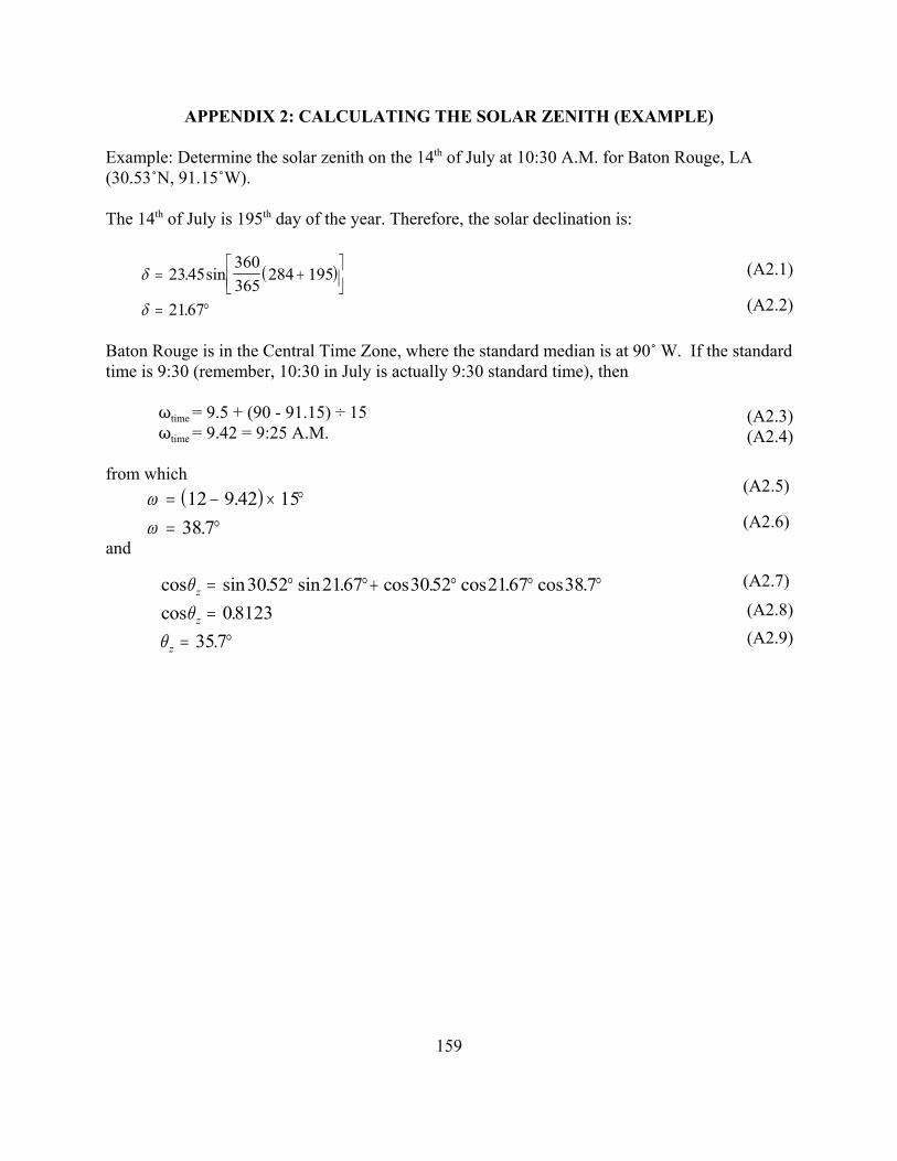
159

(A2.2)

(A2.3)(A2.4)

(A2.5)

(A2.6)

(A2.7)

(A2.8)(A2.9)

APPENDIX 2: CALCULATING THE SOLAR ZENITH (EXAMPLE)

Example: Determine the solar zenith on the 14th of July at 10:30 A.M. for Baton Rouge, LA(30.53/N, 91.15/W).

The 14th of July is 195th day of the year. Therefore, the solar declination is:

( )δ

δ

= +

= °

2345360365

284 195

2167

. sin

.

Baton Rouge is in the Central Time Zone, where the standard median is at 90/ W. If the standardtime is 9:30 (remember, 10:30 in July is actually 9:30 standard time), then

Ttime = 9.5 + (90 - 91.15) ÷ 15Ttime = 9.42 = 9:25 A.M.

from which( )ω

ω= − × °= °

12 9 42 1538 7

..

and

cos sin . sin . cos . cos . cos .cos .

.

θθ

θ

z

z

z

= ° °+ ° ° °=

= °

3052 2167 3052 2167 38 708123

357

(A2.1)

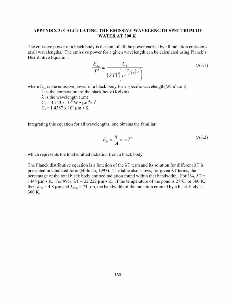
160

(A3.1)

(A3.2)

APPENDIX 3: CALCULATING THE EMISSIVE WAVELENGTH SPECTRUM OFWATER AT 300 K

The emissive power of a black body is the sum of all the power carried by all radiation emissionsat all wavelengths. The emissive power for a given wavelength can be calculated using Planck’sDistributive Equation:

( )

ET

C

T e

bC

T

λ

λλ5

1

5 12=

−

where Eb8 is the emissive power of a black body for a specific wavelength(W/m2 /:m)T is the temperature of the black body (Kelvin)8 is the wavelength (:m)

C1 = 3.743 x 10 8 W C :m4/m2

C2 = 1.4387 x 104 :m C K

Integrating this equation for all wavelengths, one obtains the familiar:

EqA

Tb = = σ 4

which represents the total emitted radiation from a black body.

The Planck distributive equation is a function of the 8T term and its solution for different 8T ispresented in tabulated form (Holman, 1997). The table also shows, for given 8T terms, thepercentage of the total black body emitted radiation found within that bandwidth. For 1%, 8T =1444 :m C K. For 99%, 8T = 22 222 :m C K. If the temperature of the pond is 27°C, or 300 K,then 81% = 4.8 :m and 899% = 74 :m, the bandwidth of the radiation emitted by a black body at300 K.

161

(A4.1)

(A4.2)

(A4.3)

(A4.4)

(A4.5)

APPENDIX 4: JUSTIFYING THE USE OF CONSTANT SURFACE TEMPERATUREAS AN APPROPRIATE BOUNDARY CONDITION IN DETERMINING THE SOIL

HEAT TRANSFER RATE

The soil was treated as a semi-infinite homogenous material when solving the heat diffusionequation:

∂∂

α∂∂

Tt

Tz

=2

2

where T is the temperature at any time and at any position within the soil," is the soil’s thermal diffusivity (a property of the soil) and z is depth below the soil surface.

One initial and two boundary conditions were required in solving the heat diffusion equation. They were:

( )T z t Tsoil initial, =(initial condition)

lim ( , )z soil zT z t T→∞ =∞=

(first boundary condition)

( )− = − −=

k ATz

hA T Tsoilz

soil pond

∂∂ 0

(second boundary condition)

where k is the soil’s thermal conductivity, A is the area of the soil surface and h is the convective heat transfer coefficient.

However, the second boundary condition required the heat transfer coefficient (h) to be known. Because of this, it was desirable to replace the second boundary condition with the followingboundary condition:

( )T z t Tpond= ≈0,(alternate second boundary condition)

This approximation could be made if the heat transfer rate between the pond and the soil wasmainly a function of the thermal properties of the soil. The Biot number (Bi) is a convenientdimensionless number which compares the resistance to conduction and the resistance toconvection for the soil.

162

(A4.6)

(A4.7)

(A4.8)

(A4.9)

(A4.10)

BiRR

hLk

cond

conv

char

soil= =

where Rcond is the thermal resistance to conductionRconv is the thermal resistance to convectionh is the heat transfer coefficient of the water (W/m2/K)Lchar is the characteristic length of the soil (m)ksoil is the thermal conductivity of the soil (W/m/K)

The characteristic length of the soil was chosen to be the dampening depth (D) with T = 1.157 x10-5 s-1 (equation 3.39). The dampening depth for clay is 0.122 m (Van Wijk and De Vries,1966). From Table 3.7, the thermal conductivity of the soil was estimated as 2.92 W/m/K. If thesource of resistance to heat transfer is the soil’s conductance, the Biot number will be large (30). So the heat transfer coefficient is:

( )h

W m Km

W m K=×

=100 2 92

01222393 2. / /

./ /

To relate this heat transfer coefficient as a velocity, Nusselt, Prandtl and Reynolds numbers wereused. The Nusselt number (Nu) is (equation 3.48):

( )( )Nu

hLk

W m K mW m K

char

water= = =

2393 3750 614

146152/ / .

. / /

Note here that the characteristic length (Lchar) is different, and was calculated from Equation3.49. Assuming mixed laminar and turbulent conditions were present, Equation 3.54 was used todetermine the Reynolds number (Re) (the Prandlt number (Pr) is 5.85 when the watertemperature is at 26°C; Holman, 1997):

Re Pr.

/

/

=+

=

Nu1 3

5 4

871

0 0375388535

Finding the velocity using Equation 3.55 yielded:

( )( )( )

VL

kg m skg m m

m schar

= =×

=−Re . / /

. / .. /

µρ

5388535 8 6 109958 375

1244

3

163

If the velocity of the water at the soil surface is faster than 0.36 m/s, then the Biot number islarge enough to assume that resistance to conduction is limiting the overall heat transfer rate.

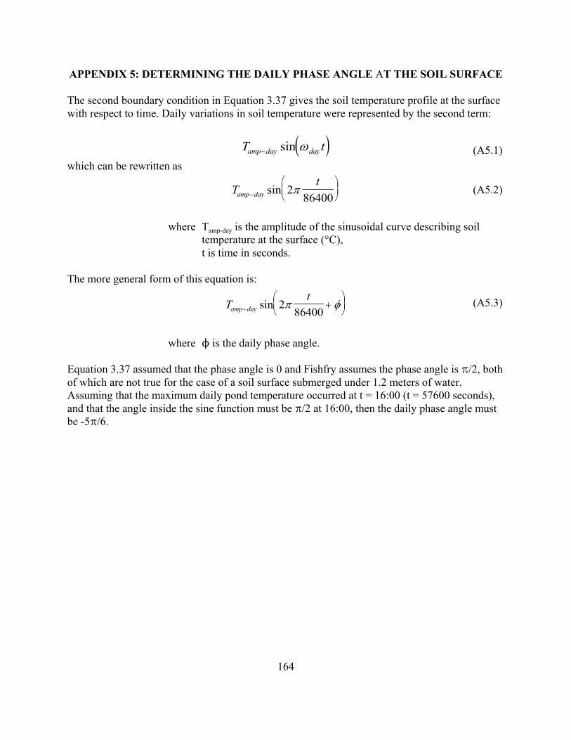
164

(A5.1)

(A5.2)

(A5.3)

APPENDIX 5: DETERMINING THE DAILY PHASE ANGLE AT THE SOIL SURFACE

The second boundary condition in Equation 3.37 gives the soil temperature profile at the surfacewith respect to time. Daily variations in soil temperature were represented by the second term:

( )T tamp day day− sin ωwhich can be rewritten as

Tt

amp day−

sin 2

86400π

where Tamp-day is the amplitude of the sinusoidal curve describing soiltemperature at the surface (°C), t is time in seconds.

The more general form of this equation is:

Tt

amp day− +

sin 2

86400π φ

where N is the daily phase angle.

Equation 3.37 assumed that the phase angle is 0 and Fishfry assumes the phase angle is B/2, bothof which are not true for the case of a soil surface submerged under 1.2 meters of water. Assuming that the maximum daily pond temperature occurred at t = 16:00 (t = 57600 seconds),and that the angle inside the sine function must be B/2 at 16:00, then the daily phase angle mustbe -5B/6.

165

(A6.1a)(A6.1b)

( )( )

Nu f

Sh f Sc

n

n

=

=1

2

Re Pr

Re(A6.2a)(A6.2b)

(A6.3)

(A6.4)

(A6.5)

APPENDIX 6: THEORY BEHIND THE DETERMINATION OF TRANSPORTCOEFFICIENTS - ANALYTICAL METHOD

(Source: Incropera and De Witt, 1985. Fundamentals of Heat and Mass Transfer 2nd edition ,page 284.)

The theory relating the convective heat transfer coefficient (h) and the convective mass transfercoefficient (hm) relies on boundary layer theory. Both the concentration and thermal boundarylayers are similar in shape and are determined by the velocity boundary layer. Both use thediffusion equation and both can be calculated using analogous empirical equations.

( )( )

Nu fSh f Sc

=

=1

2

Re,Pr

Re,

Normally, Pr and Sc are related to Nu and Sh by powers of some quantity n.

The Reynolds number (Re) is the same for both functions because both functions are subjected tothe same geometry,

( ) ( )f f1 2Re Re=so...

Nu ShSc

NuSh Sc

Len n

n

nn

PrPr

= ⇒ = = −

and...

NuSh

hLkh LD

hhDk

Le

c

fluid

m c

AB

m

AB

fluid

n= = = −

By definition, the Lewis number is thermal diffusivity divided by the mass diffusivity.

166

(A6.6)

(A6.7)

(A6.8)

( )h h c Lem pn= −ρ 1

LeD

kc DAB

fluid

fluid p fluid AB

= =−

αρ

Rearranging the terms gives:

( )Dk

c LeAB

fluidfluid p fluid= −

−ρ

1

Substituting A6.7 into equation A6.5, andisolating for hm gives Equation 5.1:

167

(A7.1)

(A7.2)( )h h c Lem pn= −ρ 1

( )&m h A C Cwater m water air= − (A7.3)

(A7.4)&m h A MM

RPT

PTwater m

water air

=

−

(A7.5)

(A7.6)

APPENDIX 7: DERIVATION OF EQUATION 5.3

Given Equation 3.4:

dEdt

q q q q q q q q q qpond

solar back sky conv evap soil rain seep well out

= − + ± − ± + − + −

d Ed t q q q q q q q q q qp o n d s o l a r b a c k s k y s o i l s e e p r a i n w e l l o u t e v a p c o n v = − + ± − + + − − ±

and given Equation 5.1

one can solve for hm. Consider Fick’s law of diffusion:

where m’water is the evaporation rate, hm is the convective mass transfer coefficient, A is the area, Cwater is the concentration of water vapour at the pond surface andCair is the concentration of water vapour in the air.

Using the perfect gas law, Equation A7.3 can be rewritten as

where MM is the molar mass of water, R is the universal gas constant, P is the pressure of the water vapour and T is the absolute temperature.

The energy lost to evaporation is:

q h m h h A MMR

PT

PTevap fg fg m

water air

= =

−

&

Newton’s law of cooling is used to predict the heat lost by convection.

( )q hA T Tconv air pond= −

168

(A7.7)

( )

( )h

dEdt

q q q q q q q q

A Le c T T hMMR

PT

PT

mpond

solar back sky soil seep rain well out

air p air air pond fgsurface air

=

− − + ± − + + −

− −

−

−

2 3/ ρ

(A7.8)

Using Equation A7.2, Equation A.6 becomes

( ) ( )q h c Le A T Tconv m p airn

air water= −−ρ 1

Substituting A7.5 and A7.7 into A7.1, and then isolating hm, one gets Equation 5.3

169

Figure A8.1: A pyranometer,similar to this one, was usedto measure solar radiationunder water.

(d)

(a)

(b)(c)(d)

(a)

(b)(c)

Figure A8.2: The pyranometer (a) was connected tothe data logger ( c) with the use of a coaxial wire (b).The inner wire was connected to the high lead whilethe outer shield was connected to the low lead. A 147Ohm resistor (d) was also connected across the datalogger terminal.

APPENDIX 8: PYRANOMETER INFORMATION

A pyranometer sensor (LI-COR LI-200SZ ) was used to measure the solar radiation below thewater surface. The sensor, shown below, had a coaxial cable with the inner cable being thepositive lead and the outer cable being the negative lead. Because the pyranometer produced acurrent signal, it was necessary to use a 147-Ohm resistor to convert this signal into a voltagesignal (schematic in Figure A8.2).

A data logger (Campbell Scientific 21X, Campbell Scientific Inc., North Logan, UT) was usedas an output device so that measurements could be read. The following program was enteredinto the data logger. Measurements were recorded so that the LI-COR pyranometer could becalibrated to an Eppley Radiometer (model PSP).

;{21X};*Table 1 Program 01: 1 Execution Interval (seconds)

1: Volt (Diff) (P2) 1: 1 Reps 2: 3 50 mV Slow Range 3: 2 DIFF Channel 4: 1 Loc [ small ] 5: 99.8 Mult

6: 0.0 Offset

170

2: Volt (Diff) (P2) 1: 1 Reps 2: 3 50 mV Slow Range 3: 3 DIFF Channel 4: 2 Loc [ big ] 5: 115.7 Mult 6: 0.0 Offset

3: If time is (P92) 1: 0 Minutes into a 2: 1 Minute Interval 3: 10 Set Output Flag High

4: Real Time (P77) 1: 1220 Year,Day,Hour/Minute (midnight = 2400)

5: Sample (P70) 1: 2 Reps 2: 1 Loc [ small ]

6: Batt Voltage (P10) 1: 3 Loc [ batery ]

*Table 2 Program 02: 0 Execution Interval (seconds)

*Table 3 Subroutines

End Program

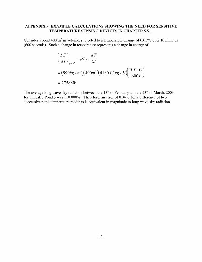
171

APPENDIX 9: EXAMPLE CALCULATIONS SHOWING THE NEED FOR SENSITIVETEMPERATURE SENSING DEVICES IN CHAPTER 5.5.1

Consider a pond 400 m3 in volume, subjected to a temperature change of 0.01°C over 10 minutes(600 seconds). Such a change in temperature represents a change in energy of

( )( )( )

∆∆

∆∆

Et

cTt

kg m m J kg KCs

W

pondp

o

= ∀

=

=

ρ

990 400 41800 01600

27588

3 3/ / /.

The average long wave sky radiation between the 13th of February and the 23rd of March, 2003for unheated Pond 3 was 110 000W. Therefore, an error of 0.04°C for a difference of twosuccessive pond temperature readings is equivalent in magnitude to long wave sky radiation.

172

APPENDIX 10: DATA LOGGER PROGRAMS

The following basic program was used to measure the pond temperature a data logger (CampbellScientific 21X, Campbell Scientific Inc., North Logan, UT). The multiplier in InstructionP:14(7) and the offset in Instruction P:14(8) were used to calibrate the thermocouple readings, soas to avoid additional manipulations during the analysis of data.

;{21X};*Table 1 Program 01: 60 Execution Interval (seconds)1: Internal Temperature (P17) 1: 1 Loc [ ref_temp ]

2: Thermocouple Temp (DIFF) (P14) 1: 1 Reps 2: 1 5 mV Slow Range 3: 1 DIFF Channel 4: 1 Type T (Copper-Constantan) 5: 1 Ref Temp (Deg. C) Loc [ ref_temp ] 6: 2 Loc [ soil_far ] 7: 1.008 Mult 8: -.016 Offset

3: Thermocouple Temp (DIFF) (P14) 1: 1 Reps 2: 1 5 mV Slow Range 3: 2 DIFF Channel 4: 1 Type T (Copper-Constantan) 5: 1 Ref Temp (Deg. C) Loc [ ref_temp ] 6: 3 Loc [ bot_far ] 7: 1.008 Mult 8: -.016 Offset

4: Thermocouple Temp (DIFF) (P14) 1: 1 Reps 2: 1 5 mV Slow Range 3: 3 DIFF Channel 4: 1 Type T (Copper-Constantan) 5: 1 Ref Temp (Deg. C) Loc [ ref_temp ] 6: 4 Loc [ high_far ] 7: 1.020 Mult 8: -.136 Offset

173

5: Thermocouple Temp (DIFF) (P14) 1: 1 Reps 2: 1 5 mV Slow Range 3: 4 DIFF Channel 4: 1 Type T (Copper-Constantan) 5: 1 Ref Temp (Deg. C) Loc [ ref_temp ] 6: 5 Loc [ sur_far ] 7: 1.008 Mult 8: -.016 Offset

6: Thermocouple Temp (DIFF) (P14) 1: 1 Reps 2: 1 5 mV Slow Range 3: 5 DIFF Channel 4: 1 Type T (Copper-Constantan) 5: 1 Ref Temp (Deg. C) Loc [ ref_temp ] 6: 6 Loc [ soil_near ] 7: 1.005 Mult 8: .034 Offset

7: Thermocouple Temp (DIFF) (P14) 1: 1 Reps 2: 1 5 mV Slow Range 3: 6 DIFF Channel 4: 1 Type T (Copper-Constantan) 5: 1 Ref Temp (Deg. C) Loc [ ref_temp ] 6: 7 Loc [ bot_near ] 7: 1.010 Mult 8: 0 Offset

8: Thermocouple Temp (DIFF) (P14) 1: 1 Reps 2: 1 5 mV Slow Range 3: 7 DIFF Channel 4: 1 Type T (Copper-Constantan) 5: 1 Ref Temp (Deg. C) Loc [ ref_temp ] 6: 8 Loc [ high_near ] 7: 1.008 Mult 8: 0.017 Offset

9: Thermocouple Temp (DIFF) (P14) 1: 1 Reps 2: 1 5 mV Slow Range 3: 8 DIFF Channel

174

4: 1 Type T (Copper-Constantan) 5: 1 Ref Temp (Deg. C) Loc [ ref_temp ] 6: 9 Loc [ sur_near ]

7: 1.005 Mult 8: 0.101 Offset

10: Batt Voltage (P10) 1: 10 Loc [ battery ]

11: If time is (P92) 1: 0 Minutes into a 2: 10 Minute Interval 3: 10 Set Output Flag High

12: Real Time (P77) 1: 1220 Year,Day,Hour/Minute (midnight = 2400)

13: Sample (P70) 1: 10 Reps 2: 1 Loc [ ref_temp ]

*Table 2 Program 02: 0.0000 Execution Interval (seconds)

*Table 3 Subroutines

End Program

If in addition to 8 thermocouples an anemometer is being used, the following program should beentered into the data logger.

*Table 1 Program 01: 60 Execution Interval (seconds)1: Internal Temperature (P17) 1: 1 Loc [ ref_temp ]

2: Thermocouple Temp (DIFF) (P14) 1: 1 Reps 2: 1 5 mV Slow Range 3: 1 DIFF Channel 4: 1 Type T (Copper-Constantan)

5: 1 Ref Temp (Deg. C) Loc [ ref_temp ]

175

6: 2 Loc [ soil_far ] 7: 0.988 Mult 8: .544 Offset

3: Thermocouple Temp (DIFF) (P14) 1: 1 Reps 2: 1 5 mV Slow Range 3: 2 DIFF Channel 4: 1 Type T (Copper-Constantan) 5: 1 Ref Temp (Deg. C) Loc [ ref_temp ] 6: 3 Loc [ bot_far ] 7: 1.002 Mult 8: .154 Offset

4: Thermocouple Temp (DIFF) (P14) 1: 1 Reps 2: 1 5 mV Slow Range 3: 3 DIFF Channel 4: 1 Type T (Copper-Constantan) 5: 1 Ref Temp (Deg. C) Loc [ ref_temp ] 6: 4 Loc [ high_far ] 7: 1.004 Mult 8: .385 Offset

5: Thermocouple Temp (DIFF) (P14) 1: 1 Reps 2: 1 5 mV Slow Range 3: 4 DIFF Channel 4: 1 Type T (Copper-Constantan) 5: 1 Ref Temp (Deg. C) Loc [ ref_temp ] 6: 5 Loc [ sur_far ] 7: .997 Mult 8: .25 Offset

6: Thermocouple Temp (DIFF) (P14) 1: 1 Reps 2: 1 5 mV Slow Range 3: 5 DIFF Channel 4: 1 Type T (Copper-Constantan) 5: 1 Ref Temp (Deg. C) Loc [ ref_temp ] 6: 6 Loc [ soil_near ] 7: 1.033 Mult 8: -.905 Offset

176

7: Thermocouple Temp (DIFF) (P14) 1: 1 Reps 2: 1 5 mV Slow Range 3: 6 DIFF Channel 4: 1 Type T (Copper-Constantan) 5: 1 Ref Temp (Deg. C) Loc [ ref_temp ] 6: 7 Loc [ bot_near ]

7: 1.028 Mult 8: -.834 Offset

8: Thermocouple Temp (DIFF) (P14) 1: 1 Reps 2: 1 5 mV Slow Range 3: 7 DIFF Channel 4: 1 Type T (Copper-Constantan) 5: 1 Ref Temp (Deg. C) Loc [ ref_temp ] 6: 8 Loc [ high_near ] 7: 1.013 Mult 8: -.218 Offset

9: Thermocouple Temp (DIFF) (P14) 1: 1 Reps 2: 1 5 mV Slow Range 3: 8 DIFF Channel 4: 1 Type T (Copper-Constantan) 5: 1 Ref Temp (Deg. C) Loc [ ref_temp ] 6: 9 Loc [ sur_near ] 7: .988 Mult 8: 1.265 Offset

10: Batt Voltage (P10) 1: 10 Loc [ battery ]

11: Pulse (P3) 1: 1 Reps 2: 2 Pulse Input Channel 3: 21 Low Level AC, Output Hz 4: 11 Loc [ wind ] 5: 0.75 Mult 6: .2 Offset

12: If time is (P92) 1: 0 Minutes into a

177

2: 10 Minute Interval 3: 10 Set Output Flag High

13: Real Time (P77) 1: 1220 Year,Day,Hour/Minute (midnight = 2400)

14: Sample (P70) 1: 10 Reps 2: 1 Loc [ ref_temp ]

15: Average (P71) 1: 1 Reps 2: 11 Loc [ wind ]

*Table 2 Program 02: 0.0000 Execution Interval (seconds)

*Table 3 Subroutines

End Program

If, in addition to 8 thermocouples a weather vane is being use, the following program should beentered into the datalogger:

;{21X};*Table 1 Program 01: 60 Execution Interval (seconds)1: Internal Temperature (P17) 1: 1 Loc [ ref_temp ]

2: Thermocouple Temp (DIFF) (P14) 1: 1 Reps 2: 1 5 mV Slow Range 3: 1 DIFF Channel 4: 1 Type T (Copper-Constantan) 5: 1 Ref Temp (Deg. C) Loc [ ref_temp ] 6: 2 Loc [ soil_far ] 7: 1.01 Mult 8: -.269 Offset

3: Thermocouple Temp (DIFF) (P14) 1: 1 Reps

2: 1 5 mV Slow Range

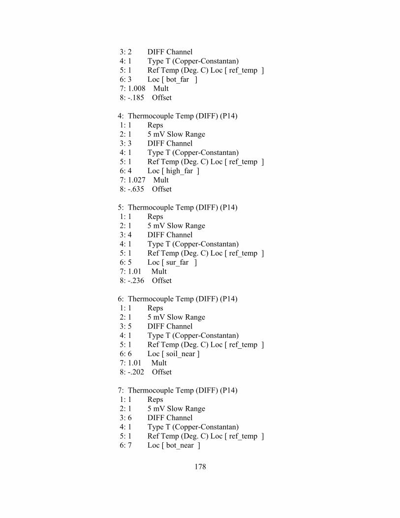
178

3: 2 DIFF Channel 4: 1 Type T (Copper-Constantan) 5: 1 Ref Temp (Deg. C) Loc [ ref_temp ] 6: 3 Loc [ bot_far ] 7: 1.008 Mult 8: -.185 Offset

4: Thermocouple Temp (DIFF) (P14) 1: 1 Reps 2: 1 5 mV Slow Range 3: 3 DIFF Channel 4: 1 Type T (Copper-Constantan) 5: 1 Ref Temp (Deg. C) Loc [ ref_temp ] 6: 4 Loc [ high_far ] 7: 1.027 Mult 8: -.635 Offset

5: Thermocouple Temp (DIFF) (P14) 1: 1 Reps 2: 1 5 mV Slow Range 3: 4 DIFF Channel 4: 1 Type T (Copper-Constantan) 5: 1 Ref Temp (Deg. C) Loc [ ref_temp ] 6: 5 Loc [ sur_far ] 7: 1.01 Mult 8: -.236 Offset

6: Thermocouple Temp (DIFF) (P14) 1: 1 Reps 2: 1 5 mV Slow Range 3: 5 DIFF Channel 4: 1 Type T (Copper-Constantan) 5: 1 Ref Temp (Deg. C) Loc [ ref_temp ] 6: 6 Loc [ soil_near ] 7: 1.01 Mult 8: -.202 Offset

7: Thermocouple Temp (DIFF) (P14) 1: 1 Reps 2: 1 5 mV Slow Range 3: 6 DIFF Channel 4: 1 Type T (Copper-Constantan) 5: 1 Ref Temp (Deg. C) Loc [ ref_temp ]

6: 7 Loc [ bot_near ]

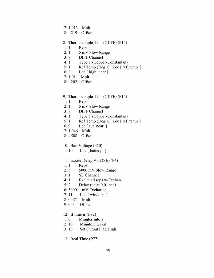
179

7: 1.013 Mult 8: -.219 Offset

8: Thermocouple Temp (DIFF) (P14) 1: 1 Reps 2: 1 5 mV Slow Range 3: 7 DIFF Channel 4: 1 Type T (Copper-Constantan) 5: 1 Ref Temp (Deg. C) Loc [ ref_temp ] 6: 8 Loc [ high_near ] 7: 1.01 Mult 8: -.202 Offset

9: Thermocouple Temp (DIFF) (P14) 1: 1 Reps 2: 1 5 mV Slow Range 3: 8 DIFF Channel 4: 1 Type T (Copper-Constantan) 5: 1 Ref Temp (Deg. C) Loc [ ref_temp ] 6: 9 Loc [ sur_near ] 7: 1.046 Mult 8: -.508 Offset

10: Batt Voltage (P10) 1: 10 Loc [ battery ]

11: Excite Delay Volt (SE) (P4) 1: 1 Reps 2: 5 5000 mV Slow Range 3: 1 SE Channel 4: 1 Excite all reps w/Exchan 1 5: 2 Delay (units 0.01 sec) 6: 5000 mV Excitation 7: 11 Loc [ winddir ] 8: 0.071 Mult 9: 0.0 Offset

12: If time is (P92) 1: 0 Minutes into a 2: 10 Minute Interval 3: 10 Set Output Flag High

13: Real Time (P77)

180

1: 1220 Year,Day,Hour/Minute (midnight = 2400)

14: Sample (P70) 1: 10 Reps 2: 1 Loc [ ref_temp ]

15: Average (P71) 1: 1 Reps 2: 11 Loc [ winddir ]

*Table 2 Program 02: 0.0000 Execution Interval (seconds)

*Table 3 Subroutines

End Program

181

3600.0000000000 step size (s)31104000.0000000000 Initial time (s)

17.0000000000 Pond temperature (/C)33609600.0000000000 Upper time limit (s) 480.0000000000 Pond Volume (m^3) 394.0000000000 Pond area (m^2) 990.0000000000 Water density (kg/m^3) 4180.0000000000 Specific heat of water (J/kg/C) 0.9599999785 Water emissivity (decimal) 0.0000005500 thermal diffusivity (m^2/s) 1.0000000000 soil density (kg/m^3) 2900000.0953674316 specific heat (J/kg/C) 5.6999998093 soiltempamp_year (/C) 5.0000000000 soiltempamp_day (/C) 1.5707963705 phase_year (radians) 1.5707963705 phase_day (radians)

Figure A11.1: The required layout for the information.dat file.

APPENDIX 11: HOW TO USE FISHFRY

To use Fishfry, the following 4 ASCII data files must be available to the executive program inthe same directory:

• information.dat: lists all the soil and pond parameters as well as the initial conditions. The file must have the following layout, although the numeric valuescan change.

• weather.dat: lists all the weather data for a certain time step specified ininformation.dat. This ASCII file contains 8 columns. The first 3 are arbitrarynumbers (usually the year, day of the year and time). The forth column is for theair temperature (°C), the fifth is for relative humidity (a number between 1 and100), the sixth is for solar radiation (kW/m2), the seventh is for wind speed (m/s),the eight is for rainfall (inches/hr).

• flow.dat: this is a 5 column ASCII file. The first 3 are arbitrary numbers (usuallythe year, day of the year and time). The forth column lists the flow rate of warmwater into the pond. The fifth column lists the flow rate of cold water into thepond.

• temp.dat: this is a 1 column ASCII file which lists the pond temperature (°C). This is for cases when the user is interested in knowing the flow rate of water

182

Welcome to FISHFRY, the easy way to know how much heat youneed to supply to the pond so that your fish won't freeze or cook.

Please remember to include the following files in the FISHFRYdirectory/folder before running the program:

- information.dat - weather.dat - flow.dat - temp.dat The output file will be called output.dat, where columns are spaceseperated, and easily viewed in your favorite spreadsheet. Press any number to continue

What do you want FISHFRY to do?Please enter the appropriate number.

(1) Determine the flow rate of water into the pond to maintain a desired pond temperature.

(2) Determine the temperature of a pond given the flow rate and weather.

(0) End FISHFRY, the best program in the whole wide world.

Figure A11.2: The Fishfry User Prompt is accessed from DOS.

needed to maintain his pond temperature at a certain value (used only for option1).

Once these files are available in the home directory, the user can run Fishfry.exe. After startingthe program, the following prompt will appear:

Once the user has selected one of these choice, the model will prompt the user for a name for theoutput file, the initial pond temperature (°C), the temperature of the warm water at the inlet (°C),the temperature of the cold water at the inlet (°C), the name of the weather file and the name ofthe pond temperature file. If no warm or cold water is being used, enter 0 when asked for thetemperature.

Fishfry will then compile results. Sometimes, Fishfry will give out an error statement at the endof a model run. This happened because there was not enough input information for the defined

183

time period (defined in information.dat). The user must make sure the number of input data in afile is equal to the number of time steps.

Once the program is finished, the user can open the output file in a spreadsheet program as aASCII file with comma separated variables.

184

APPENDIX 12: PROGRAM CODE FOR FISHFRY

PROGRAM fishfryIMPLICIT NONE

!====================================================================! INTRODUCTION!------------------------------------------------------------------------------!! Fishfry v 1.2 is the master version of Fishfry which includes some! some of the suggested modifications made in chapter 4. Although! equations for the effects of soil heat transfer are present, they! have been made idle due to their small contribution to the overall! pond energy balance.!! This version of Fishfry has two modes. The first is more practicle! for managing the supply of cool and warm water. For a given pond! temperature, which can be made to varry in the temp.dat input file,! Fishfry will calculate the amount of cold and warm water required to! keep the pond at that given temperature.!! The second Fishfry mode is more useful for validating the model,! although it can be used as a management tool. Fishfry, in mode 2,! will solve for the pond temperature given all the energy fluxes.!!====================================================================! FUNCTIONS!------------------------------------------------------------------------------! dTemp - Differential Equation!! The following interface evaluates dTemp for a given temp and time, using! the 4th order Runge Kutta numerical method

InterfaceFUNCTION dTemp(Temp,time,coefficient,thermal_mass, airtemp) !step)IMPLICIT NONE REAL (8), INTENT (IN):: Temp, time, thermal_mass, airtemp !, step REAL (8), dimension (10), INTENT (IN):: coefficient REAL (8):: dTempEND function dTempEND interface

!------------------------------------------------------------------------------! emissivity_sky

185

!! The following interface evaluates the emissivity of a clear sky.

InterfaceFunction emissivity_sky(airtemp,rh)Implicit NONE

REAL (8), INTENT(IN):: airtemp, rhrEAL (8):: emissivity_sky

END function emissivity_skyend interface

!------------------------------------------------------------------------------! vapour pressure!! The following interface is for a function which evaluates the vapour! pressure in Pascals.!

InterfaceFUNCTION vp(T, rh)IMPLICIT NONeREAL (8), INTENT (IN):: T, rhREAL (8):: vpeND function vpend Interface

!------------------------------------------------------------------------------! Wind speed correction function - REQUIRES AN INPUT!!! The following interface is for a function which corrects wind speed for! the Lake Hefner equation. It also converts units from m/s to mph.!

Interfacefunction ws(windspeed)implicit noneREAL (8), INTENT (IN):: windspeedREAL (8):: wsend function wsEND interface

!

186

!====================================================================! VARIABLE DECLARATIONS!------------------------------------------------------------------------------! Runge Kutta variables

REAL (8):: F1, F2, F3, F4REAL (8):: Temp, time, step, timemax

! Temp: pond temperature (C)! time: time (sec)! step: time step (sec)! timemax: upper integration limit (sec)! F1, F2, F3, F4: integration formulae for Runge-Kutta!!------------------------------------------------------------------------------! Pond parameters

REAL(8):: volume, area, density, specheat, Thermal_mass, emissivity_water

! Volume: pond volume (m^3)! Area: pond surface area (m^2)! density: density of pond water (kg/m^3)! specheat: specific heat of water (J/kg/C)! Thermal_mass: Volume*density*specfic heat (J/C)! emissivity_water: emissivity of the water!!------------------------------------------------------------------------------! Flux parameters

REAL(8):: latent_energyREAL(8):: flow_rate_hot, flow_rate_cold, gpm_hot, gpm_cold, hot, cold

! latent_energy: energy for the vapourization of water! hot: the temperature of the warm influent (C)! cold: the temperature of the cold influent (C)! flow_rate_hot: the flow rate of the warm effluent (m^3/s)! flow_rate_cold: the flow rate of the cold effluent (m^3/s)! gpm_hot:: the flow rate of the warm effluent (gpm)! gpm_cold: the flow rate of the cold effluent (gpm)!!------------------------------------------------------------------------------! Atmospheric parameters

187

REAL (8):: airtemp, rh, windspeed, solar_radiation, x, rain!, winddirection

! emissivity_sky: emissivity in the sky (decimal)! airtemp: air temperature (C)! rh: relative humidity (demical)! solar_radiation: solar_radiation (J/m^2/s)! windspeed: wind speed (mph)

! wind direction: degrees, 0 = North! x: relative humidity of 100% (1)!!------------------------------------------------------------------------------! Soil parameters!!Real(8):: thermal_conductivity, thermal_diffusivity, soil_density!REAL(8):: cp_soil, Dday, Dyear, temp_initial, PI!REAL(8):: Soiltempamp_year, Soiltempamp_day, phase_year, phase_day

!! thermal conductivity: J/m/C/s (Fourier's heat conduction law)! thermal diffusivity: m^2/s (Heat diffusion equation)! Soil_density: kg/m^3! cp_soil: Soil specific heat (J/kg/C)! Dday: dampening depth for daily variations (m)! Dyear: dampening depth for yearly variations (m)! temp_initial: initial soil temperature (/C)! Soiltempamp_year: The yearly amplitude for soil temperature (/C)! Soiltempamp_day: The daily amplitude for soil temperature (/C)! phase_year: phase angle for the year! phase_day: phase angle for the day! PI!!------------------------------------------------------------------------------! Coefficient arrays!

REAL(8), dimension (10):: coefficient, vector

! Coefficient (1): coefficient for pond longwave radiation! Coefficient (2): coefficient for atmospheric longwave radiation! Coefficient (3): coefficient for soil heat exchange! Coefficient (4): coefficient for surface evaporation! Coefficient (5): coefficient for surface convection! Coefficient (6): coefficient for penetrated solar radiation

188

! Coefficient (7): coefficient for warm water inlet

! Coefficient (8): coefficient for cold water inlet! Coefficient (9): coefficient for discharge!! Vector (1): Power due to pond longwave radiation! Vector (2): Power due to atmospheric longwave radiation! Vector (3): Power due to soil heat exchange! Vector (4): Power due to surface evaporation! Vector (5): Power due to surface convection! Vector (6): Power due to solar radiation! Vector (7): Energy flow in the hot water! Vector (8): Energy flow in the cold water! Vector (9): Energy flow in the discharge!! All vector terms are in Joules/second (Watts)!!------------------------------------------------------------------------------! Other parameters!

integer:: choiceCHARACTER(LEN=12):: weather_file, temp_file, pond!!====================================================================! FILES AND FORMAT!------------------------------------------------------------------------------

OPEN (99, FILE="information.dat") ! Information input data file!OPEN (100, FILE="output.dat") ! Output data file!OPEN (200, FILE="weather.dat") ! Input air temperature data fileOPEN (300, FILE="flow.dat") ! Flow input!OPEN (400, FILE="temp.dat") ! Pond Temperature input

10 FORMAT (20(f30.6, ","), f30.6)20 FORMAT (20(a30, ","), a30)

!====================================================================! SETTING OF PARAMETERS (USER REQUIRED INPUT HERE)!------------------------------------------------------------------------------! Initial conditions

189

READ (99,*) step ! Step size (s)Read (99,*) time ! Initial time(s)Read (99,*) temp ! Initial pond water temperature (C)Read (99,*) timemax ! Upper limit for time (s)

!!------------------------------------------------------------------------------! Properties of the pond

Read (99,*) Volume ! in m^3Read (99,*) Area ! in m^2

Read (99,*) Density ! in kg/m^3Read (99,*) Specheat ! in J/kg/C

Thermal_mass = Volume*Density*Specheat

Read (99,*) Emissivity_water ! decimalx = 1.0 ! constant (no input here)!PI=ACOS(-1.0) ! the value of pi!------------------------------------------------------------------------------! Properties of the liner (soil)!

!read (99,*) thermal_diffusivity ! soil thermal diffusivity (m^2/s)!read (99,*) soil_density ! bulk soil density (kg/m^3)!read (99,*) cp_soil ! soil specific heat (J/kg/C)!read (99,*) Soiltempamp_year ! Yearly soil amplitude (/C)!read (99,*) Soiltempamp_day ! Daily soil amplitude (/C)!read (99,*) phase_year ! Phase angle, year (radians)!read (99,*) phase_day ! Phase angle, day (radians)

!temp_initial=temp!Thermal_conductivity=thermal_diffusivity*(soil_density*cp_soil)!Dday=SQRT(2.0*thermal_conductivity/soil_density/cp_soil*86400.0/2/PI)!Dyear=SQRT(2.0*thermal_conductivity/soil_density/cp_soil*31536000.0/2/PI)

!!====================================================================! User prompt to determine if the pond is at steady state or transient.

190

!write (*,*) "Welcome to FISHFRY, the easy way to know how much heat you need"write (*,*) "to supply to the pond so that your fish won't freeze or cook."write (*,*) " "write (*,*) "Please remember to include the following files in the FISHFRY"write (*,*) "directory/folder before running the program: "write (*,*) " "write (*,*) " - information.dat "write (*,*) " - weather.dat"write (*,*) " - flow.dat"write (*,*) " - temp.dat"write (*,*) " "write (*,*) "The output file will be called output.dat, where columns are space"write (*,*) "seperated, and easily viewed in your favorite spreadsheet."write (*,*) " "write (*,*) "Press any number to continue"write (*,*) " "READ (*,*) choice

111 write (*,*) "What do you want FISHFRY to do?"write (*,*) "Please enter the appropriate number."write (*,*) " "write (*,*) " (1) Determine the flow rate of water into the pond to maintain"write (*,*) " a desired pond temperature."write (*,*) " "write (*,*) " (2) Determine the temperature of a pond given the flow rate"write (*,*) " and weather."write (*,*) " "write (*,*) " (0) End FISHFRY, the best program in the whole wide world."write (*,*) " "read (*,*) choice

IF (choice>2) THENwrite (*,*) "You have made an invalid choice."GO TO 111END IF

!====================================================================! SETTING INITIAL OR BOUNDARY CONDITIONS!

write (*,*) "Which pond is being considered?"write (*,*) " "read (*,*) pond

191

write (*,*) "What is the temperature of the warm influent? (C)"write (*,*) " "read (*,*) hot

write (*,*) "What is the temperature of the cool influent? (C)"write (*,*) " "read (*,*) cold

IF (choice==2) THEN

write (*,*) "What is the initial pond temperature?"write (*,*) " "read (*,*) temp

END IF

IF (choice==0) GO TO 9

WRITE (*,*) "What is the name of the weather file? "READ (*,*) weather_fileWRITE (*,*) "What is the name of the temp file? "READ (*,*) temp_file

OPEN (200, FILE=weather_file) ! Input air temperature data fileOPEN (400, FILE=temp_file) ! Flow inputopen (100, FILE=pond)

!====================================================================! HEADINGS FOR OUTPUT FILES!!WRITE (100, *) "Results from Fishfry; OUTPUT.DAT"WRITE (100, *) " "WRITE (100, *) "Pond number: ", pondWRITE (100, *) " "WRITE (100, *) "Initial day of trial: ", time/24/3600+1WRITE (100, *) "Final day of trial: ", timemax/24/3600+1WRITE (100, *) " "

WRITE (100,*) "Influent hot temperature (C): ", hot , "Type of year:", weather_fileWRITE (100,*) "Influent cold temperature (C): ", cold, "Pond Temperature:", temp_fileWRITE (100,*) " "

192

!! Case 1: Determination of flowrates!

IF (choice==1) THEN

WRITE (100,20) "Time", " ", "Pond Radiation", "Sky Radiation", "Soil Conduction", & & "Evaporation", "Convection", "Solar Radiation", "Rain", "Rain out",& & "Surplus/deficit", "Warm Water Flow", "Warm Water Flow",& & "Cool Water Flow","Cool Water Flow"

WRITE (100,20) "(seconds)","(days)", "(Watts)", "(Watts)", "(Watts)", "(Watts)", "(Watts)",& & "(Watts)", "(Watts)", "(Watts)", "(Whr)", "(m^3/s)", "(GPM)",& & "(m^3/s)", "(GPM)"

END IF

! Case 2: Determination of pond temperature

IF (choice==2) THEN

WRITE (100,20) "Time", " ", "Pond Radiation", "Sky Radiation", "Soil Conduction", & & "Evaporation", "Convection", "Solar Radiation", & & "Warm inlet", "Cold inlet", "Discharge", "Rain", "Pond Temperature"

WRITE (100,20) "(seconds)", "(days)", "(Watts)", "(Watts)", "(Watts)", "(Watts)", & & "(Watts)", "(Watts)", "(Watts)", "(Watts)", "(Watts)", "(Watts)","(/C)"

END IF

!====================================================================! CALCULATIONS AND INTEGRATION

DO

!------------------------------------------------------------------------------! Determination of the atmospheric variables!! Because the user may wish to either use recorded data or generated! weather data, all atmospheric variables will be called up from *.dat! files. The user, however, must make sure the time steps in the data! file corresponds to the time step in this program. For instance, if the! model is to simulate pond heat transfer as of March 10th, every 10

193

! minutes, then data for every 10 minutes as of March 10th are to be in! the respective *.dat file.!! In the absence of real data, the user may generate his/her own data! with the use of sinusoidal functions. For temperature approximations for! Baton Rouge, LA, the program temperature.exe, generated from the! temperature.f90 code, can be used.!! Also, MAKE SURE THAT THE DATA FILES ARE IN THE SAME DIRECTORY AS ! FISHFRY!!

read (200, *) airtemp, airtemp, airtemp, airtemp, rh, solar_radiation, windspeed, rain

! Conversions

rh=rh*0.01solar_radiation=solar_radiation*1000.0windspeed=windspeed*3600.0/1609.0 ! converts m/s to mphrain=rain/3600.0 ! converts m/hr into m/s

if (choice==1) read (400,*) tempif (choice==2) read (300,*) flow_rate_hot, flow_rate_hot, flow_rate_hot,& & flow_rate_hot, flow_rate_cold!! From these variables, all other atmospheric variables can be determined.!! Energy of vaporization

latent_energy= 2502535.259 -212.56384*temp ! J/kg

!------------------------------------------------------------------------------!! Determination of the coefficients!coefficient(1)=emissivity_water*area*5.67*(10.0**(-8))coefficient(2)=emissivity_sky(airtemp, rh)*area*5.67*(10.0**(-8))*(airtemp+273)**4

!if (choice==3) then ! For the case when the temperature is the driving force

!coefficient(3) = -thermal_conductivity * Area& ! & * (-soiltempamp_year/Dyear&

194

! & *(sin(2*acos(-1.0)/31536000.0*time+phase_year)& ! & +cos(2*acos(-1.0)/31536000.0*time+phase_year))& ! & -soiltempamp_day/Dday& ! & *(sin(2*acos(-1.0)/86400.0*time+phase_day)& ! & +cos(2*acos(-1.0)/86400.0*time+phase_day)))!!!!else ! Steady state constant temperature conditions

!coefficient(3)=thermal_conductivity*area/sqrt(PI*thermal_diffusivity)!END if!!!

coefficient(3)=0.0coefficient(4)=(0.068+0.059*ws(windspeed))*(vp(Temp, x)-vp(airtemp,rh))& & *area*density/24.0/3600.0*0.0254& ! rate of evaporation (kg/s) & *latent_energy

coefficient(5)=(2.8+3.0*windspeed*1609.0/3600.0)*areacoefficient(6)=solar_radiation*areacoefficient(7)=density*specheat*hot*flow_rate_hotcoefficient(8)=density*specheat*cold*flow_rate_coldcoefficient(9)=density*specheat*airtemp*area*rain

if (choice==1) thencoefficient(10)=density*specheat*(area*rain)elsecoefficient(10)=density*specheat*(flow_rate_hot+flow_rate_cold+area*rain)end if

!! "If" statements to make sure no evaporation occurs when the air is saturated.!if (rh>=1.0) coefficient(4)=0if (vp(airtemp,rh)>vp(Temp,x)) coefficient(4) =0!!====================================================================! DETERMINATION OF VECTORS!

195

vector(1)= - coefficient(1)*(273.0+temp)**4 ! Pond radiation (J/s)vector(2)= coefficient(2) ! Sky radiation

!if (choice==3) then ! Soil conduction (weather forcing) ! vector(3)= coefficient(3)!ELSE ! Soil conduction (temperature constant)

! vector(3)=coefficient(3)*(Temp_initial-temp)/SQRT(time)!end ifvector(3)=0.0vector(4)= - coefficient(4) ! Evaporationvector(5)= coefficient(5)*(airtemp - temp) ! Surface convectionvector(6)= coefficient(6) ! Solar Radiationvector(9)= coefficient(9) ! Rainvector(10)=-coefficient(10)*temp

if (choice==1) THEN

vector(7)=0.0 vector(8)=0.0

if (SUM(vector)<0) then flow_rate_hot=SUM(vector)/(specheat*density*(temp-hot)) gpm_hot=flow_rate_hot*1000*60/3.78 flow_rate_cold=0.0 gpm_cold=0.0 end if

if (SUM(vector)>0) then flow_rate_cold=SUM(vector)/(specheat*density*(temp-cold)) gpm_cold=flow_rate_cold*1000*60/3.78 flow_rate_hot=0.0 gpm_hot=0.0 end ifEND if

if (choice==2) then

vector(7)= coefficient(7) vector(8)= coefficient(8) vector(9)= coefficient(9) vector(10)= -coefficient(10)*temp

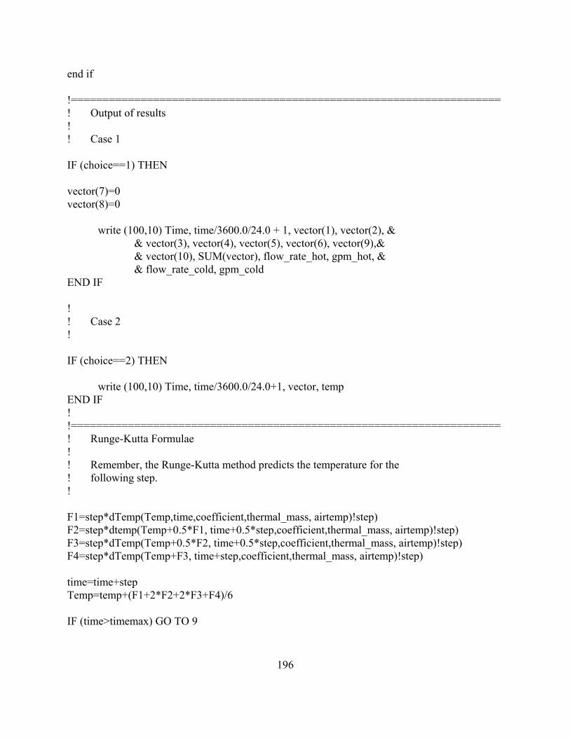
196

end if

!====================================================================! Output of results!! Case 1

IF (choice==1) THEN

vector(7)=0vector(8)=0

write (100,10) Time, time/3600.0/24.0 + 1, vector(1), vector(2), & & vector(3), vector(4), vector(5), vector(6), vector(9),& & vector(10), SUM(vector), flow_rate_hot, gpm_hot, & & flow_rate_cold, gpm_coldEND IF

!! Case 2!

IF (choice==2) THEN

write (100,10) Time, time/3600.0/24.0+1, vector, tempEND IF!!====================================================================! Runge-Kutta Formulae!! Remember, the Runge-Kutta method predicts the temperature for the! following step.!

F1=step*dTemp(Temp,time,coefficient,thermal_mass, airtemp)!step)F2=step*dtemp(Temp+0.5*F1, time+0.5*step,coefficient,thermal_mass, airtemp)!step)F3=step*dTemp(Temp+0.5*F2, time+0.5*step,coefficient,thermal_mass, airtemp)!step)F4=step*dTemp(Temp+F3, time+step,coefficient,thermal_mass, airtemp)!step)

time=time+stepTemp=temp+(F1+2*F2+2*F3+F4)/6

IF (time>timemax) GO TO 9

197

END do

9 write (*,*) "Thank you for using FISHFRY, the best program in the whole,"write (*,*) "wide world. (Quite frankly, I don't know why you would want to"write (*,*) "end your session. I mean, do you really have anything better"WRITE (*,*) "to do?)"WRITE (*,*) " "WRITE (*,*) "Results are in the output.dat file."write (*,*) " "

stopend program fishfry

!====================================================================! FUNCTIONS!====================================================================

!------------------------------------------------------------------------------! Function to evaluate dtemp!------------------------------------------------------------------------------

Function dtemp (temp, time,coefficient,thermal_mass, airtemp)IMPLICIT NONE REAL (8), INTENT (IN):: temp, time, thermal_mass, airtemp REAL (8), dimension (10), INTENT (IN):: coefficient REAL (8):: dtemp

dtemp= (& & - coefficient(1) * ((Temp+273.0)**4)& ! Backradiation & + coefficient(2) & ! Sky longwave rad & + coefficient(3) &! & + coefficient(3)*(Tsoil-temp)/SQRT(timereset)& ! Soil heat exchange & - coefficient(4)& ! Evaporation & + coefficient(5)*(airtemp-temp)& ! Convection & + coefficient(6)& ! Solar radiation & + coefficient(7)& & + coefficient(8)+coefficient(9) & & - coefficient(10)*temp& & )/thermal_mass - time+ time ! Thermal mass

ReturnEND function dtemp

198

!------------------------------------------------------------------------------! Function to evaluate emissivity_sky!------------------------------------------------------------------------------

Function emissivity_sky(airtemp,rh)IMPLICIT NONE

! This function calculates the emissivity of the sky based on a graph! produced by Bliss,1961, Atmospheric Radiation Near the Surface of! the Ground: a Summary for Engineers. Solar Energy 5:103-120!

REAL (8), INTENT(IN):: airtemp, rhREAL (8):: emissivity_sky, dewT

dewT = 1/((1/(airtemp+273))-1.846*(10.0**(-4))*LOG(rh)) - 273emissivity_sky = 1/(1.2488219 -0.0060896701*dewT+4.8502935e-005*dewT**2)

! dewT = dew temperature (C)! emissivity_sky = the sky's emissivity (decimal)

ReturnEND function emissivity_sky

!------------------------------------------------------------------------------! Function to evaluate the vapour pressure!------------------------------------------------------------------------------!! This function was taken from ASHRAE Fundamentals Handbook, 1985, SI! edition. All temperatures must be in Kelvin and all pressures are in! Pascals.

FUNCTION vp(t, rh)IMPLICIT NONEREAL (8), INTENT (IN):: T, rhREAL (8):: vp_saturated, vp

vp_saturated= exp ( -5800.2206/(t+273) & & +1.3914993 & & -0.04860239 * (t+273) & & +0.41764768 * (10.0**(-4)) * ((t+273)**2)& & -0.14452093 * (10.0**(-7)) * ((t+273)**3)& & +6.5459673 * log(t+273))

199

vp=rh*vp_saturated

vp=vp/3387 ! conversion from Pascals to inches of mercury (I HATE IMPIRIAL UNITS!!)

returnEND function vp

!------------------------------------------------------------------------------! Function to evaluate the corrected wind speed (REQUIRES INPUT!)!------------------------------------------------------------------------------

function ws(windspeed)implicit noneREAL (8), INTENT (IN):: windspeedREAL (8):: ws, height_anemometer

! This function corrects the windspeed for a height of 13 feet above! the ground. The height of the anemometer is in feet and the windspeed! in m/s. The function then converts from m/s to mph.!

height_anemometer=10.0

ws=windspeed*LOG(13.0)/LOG(height_anemometer)! conversion due to anemometer height!ws=ws*3600.0/1609.0 ! converts m/s to mph

returnend function ws

200

APPENDIX 13: PROGRAM CODE FOR WEATHER GENERATOR(A)

program weather_generatorimplicit none

interfacefunction solar(i, month, x)implicit none

INTEGER, INTENT (IN):: i, month, xREAL:: solarEND function solarEND interface

CHARACTER (LEN=20):: filename, garbageREAL, dimension (8760):: airtemp, rh, windspeedREAL, DIMENSION (8760):: airtemp_max, airtemp_min, airtemp_avgREAL, DIMENSION (8760):: rh_avg, windspeed_avgREAL, DIMENSION (8760):: solar_radiation_max, solar_radiation_minREAL, DIMENSION (8760):: solar_radiation_avg

INTEGER:: i, year, month, day, hour, j, n, choice, x

88 FORMAT (f5.1, ",", f5.0, ",", f10.5, ",", f5.1 )

!====================================================================open (300, FILE="hot.dat")open (301, FILE="cold.dat")open (302, FILE="avg.dat")

!====================================================================airtemp_max=-1000.0airtemp_min=1000.0

n=0

!====================================================================

1 n=n+1

write (*,*) "What is the name of the file?"read (*,*) filenameopen (10, FILE=filename)

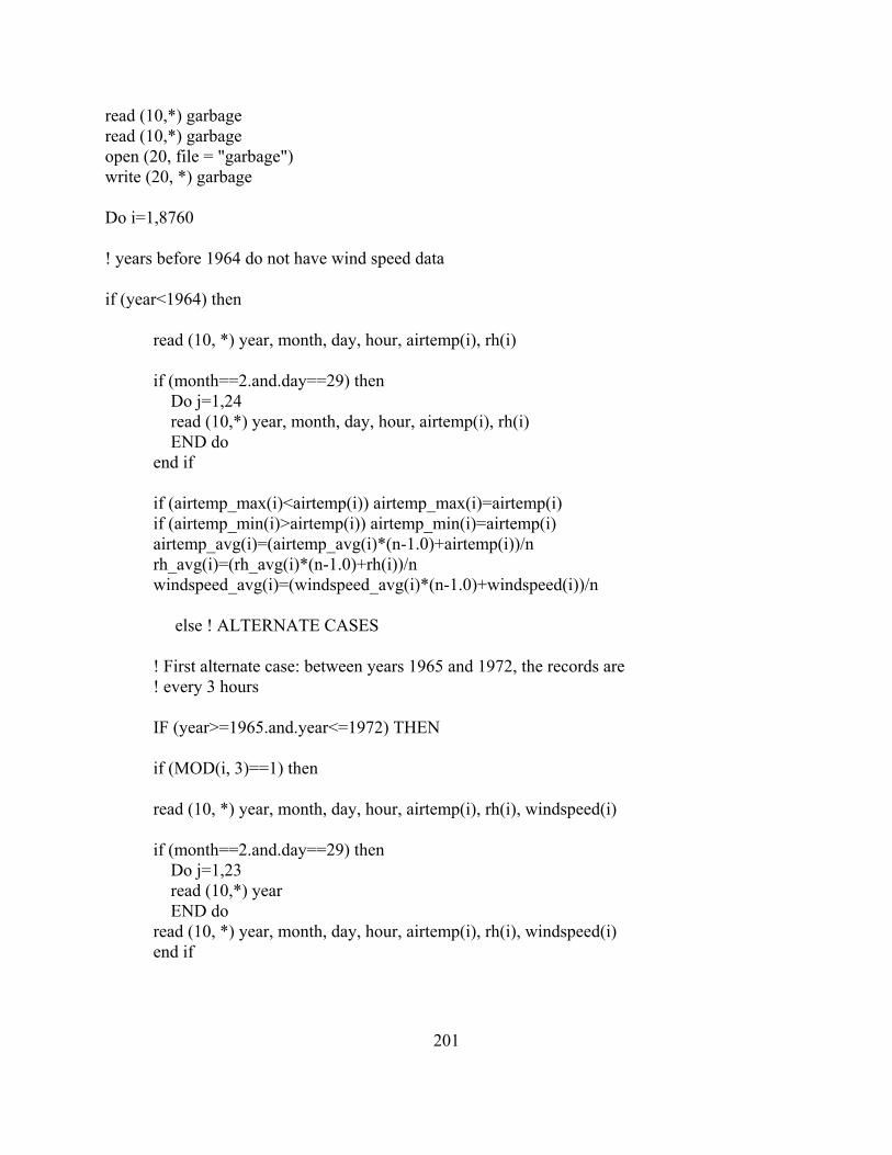
201

read (10,*) garbageread (10,*) garbageopen (20, file = "garbage")write (20, *) garbage

Do i=1,8760

! years before 1964 do not have wind speed data

if (year<1964) then

read (10, *) year, month, day, hour, airtemp(i), rh(i)

if (month==2.and.day==29) then Do j=1,24 read (10,*) year, month, day, hour, airtemp(i), rh(i) END do end if

if (airtemp_max(i)<airtemp(i)) airtemp_max(i)=airtemp(i) if (airtemp_min(i)>airtemp(i)) airtemp_min(i)=airtemp(i) airtemp_avg(i)=(airtemp_avg(i)*(n-1.0)+airtemp(i))/n rh_avg(i)=(rh_avg(i)*(n-1.0)+rh(i))/n windspeed_avg(i)=(windspeed_avg(i)*(n-1.0)+windspeed(i))/n

else ! ALTERNATE CASES

! First alternate case: between years 1965 and 1972, the records are ! every 3 hours

IF (year>=1965.and.year<=1972) THEN

if (MOD(i, 3)==1) then

read (10, *) year, month, day, hour, airtemp(i), rh(i), windspeed(i)

if (month==2.and.day==29) then Do j=1,23 read (10,*) year END do read (10, *) year, month, day, hour, airtemp(i), rh(i), windspeed(i) end if

202

if (airtemp_max(i)<airtemp(i)) airtemp_max(i)=airtemp(i) if (airtemp_min(i)>airtemp(i)) airtemp_min(i)=airtemp(i) airtemp_avg(i)=(airtemp_avg(i)*(n-1.0)+airtemp(i))/n rh_avg(i)=(rh_avg(i)*(n-1.0)+rh(i))/n windspeed_avg(i)=(windspeed_avg(i)*(n-1.0)+windspeed(i))/n

else read (10,*) year, month, day, hour airtemp(i)=airtemp(i-1) rh(i) =rh(i-1) windspeed(i) = windspeed(i-1) if (airtemp_max(i)<airtemp(i)) airtemp_max(i)=airtemp(i) if (airtemp_min(i)>airtemp(i)) airtemp_min(i)=airtemp(i) airtemp_avg(i)=(airtemp_avg(i)*(n-1.0)+airtemp(i))/n rh_avg(i)=(rh_avg(i)*(n-1.0)+rh(i))/n windspeed_avg(i)=(windspeed_avg(i)*(n-1.0)+windspeed(i))/n

END if

! Second alternate case: 1964, and 1973 onward

Else

read (10, *) year, month, day, hour, airtemp(i), rh(i), windspeed(i)

if (month==2.and.day==29) then Do j=1,24 read (10,*) year, month, day, hour, airtemp(i), rh(i), windspeed(i) END do end if

if (airtemp_max(i)<airtemp(i)) airtemp_max(i)=airtemp(i) if (airtemp_min(i)>airtemp(i)) airtemp_min(i)=airtemp(i) airtemp_avg(i)=(airtemp_avg(i)*(n-1.0)+airtemp(i))/n rh_avg(i)=(rh_avg(i)*(n-1.0)+rh(i))/n windspeed_avg(i)=(windspeed_avg(i)*(n-1.0)+windspeed(i))/n

END IFEND if

airtemp(i) = (airtemp(i)-32)*5.0/9.0airtemp_max(i) = (airtemp_max(i)-32)*5.0/9.0airtemp_min(i) = (airtemp_min(i)-32)*5.0/9.0

203

airtemp_avg(i) = (airtemp_avg(i)-32)*5.0/9.0windspeed_avg(i) = windspeed_avg(i) * 0.51444

! Solar radiation calculations

x=0solar_radiation_avg(i)=solar(i, month, x)

x=1solar_radiation_max(i)=solar(i, month, x)

x=2solar_radiation_min(i)=solar(i, month, x)

END do

WRITE (*,*) "Do you want to run an other year? (1 for yes, 2 for no) "read (*,*) choiceif (choice==1) GO TO 1

!====================================================================

DO i=1,8760 write (300,88) airtemp_max(i), rh_avg(i), solar_radiation_max(i), windspeed_avg(i) write (301,88) airtemp_min(i), rh_avg(i), solar_radiation_min(i), windspeed_avg(i) write (302,88) airtemp_avg(i), rh_avg(i), solar_radiation_avg(i), windspeed_avg(i)

END DO

stopend program weather_generator

!=====================================================================

function solar(i, month, x)implicit none

INTEGER, INTENT (IN):: i, month, x

REAL:: solar

REAL:: dy, a, piREAL:: ET, decl, rr

204

REAL:: TST, LST, Lnt, Lng, LatREAL:: HR, Elev, Directsun, etr, PETRREAL:: sunup, sundown

Lat = 30.32Lng = 91.15Lnt = 90.00pi=ACOS(-1.0)

Dy=i/24LST=1.0*MOD(i,24)

! Position of the sun

a=2*pi*dy/365.0rr=1.000110+0.034221*COS(a)+0.001280*SIN(a)+& ! ratio & 0.000719*COS(2*a)+0.000077*SIN(2*a)

ET= 0.0172+0.4281*COS(a)-7.3515*SIN(a)& ! time (min) & -3.3495*COS(2*a)-9.3619*sin(2*a)

Decl= 0.39637 -22.91326*COS(a)+4.02543*SIN(a)& ! degrees & -0.38720*COS(2*a)+0.05197*SIN(2*a)& & -0.15453*COS(3*a)+0.08479*SIN(3*a)

TST = LST +(Lnt-Lng)/15.0+ET/60.0

HR = (12.0-tst)*15 ! degrees

Elev = ASIN(SIN(pi/180*lat)*SIN(pi/180*Decl)& ! radians & +COS(pi/180*lat)*COS(pi/180*decl)*COS(pi/180*HR))

! Daylength

sundown=((180/PI*ACOS(-TAN(Lat*Pi/180)*TAN(decl*pi/180)))/15+12)-(lnt-lng)/15-et/60sunup =(12-(180/PI*ACOS(-TAN(Lat*Pi/180)*TAN(decl*pi/180)))/15)-(lnt-lng)/15-et/60! \----------hour angle------------------------/! \---------------------true solar time----------------/! \---------------------------------local standard time-------------------/

! Extra-terrestrial solar radiation

205

Directsun=1377 * rr ! Solar constant taken as 1377 W/m^2etr=Directsun/1000*COS(pi/2-elev) ! kW/m^2

if (LST<sunup.or.lst>sundown) etr=0

if (month==1) petr= 0.46if (month==2) petr= 0.50if (month==3) petr= 0.56if (month==4) petr= 0.62if (month==5) petr= 0.62if (month==6) petr= 0.63if (month==7) petr= 0.58if (month==8) petr= 0.61if (month==9) petr= 0.61if (month==10) petr= 0.64if (month==11) petr= 0.54if (month==12) petr= 0.48if (x==1) petr=0.85if (x==2) petr=0.25

solar=petr*etr

ReturnEND function solar

206

Vita

Jonathan Lamoureux was born in Montreal, Quebec, Canada, on September 28, 1978. His lovefor the outdoors, creativity and problem solving prompted him to become an agriculturalengineer. In 1997, he enrolled in the Department of Biosystems and Agricultural Engineering atMacdonald Campus, McGill University in Ste. Anne-de-Bellevue, Quebec. Four years later, heearned his Bachelor of Science degree in agricultural engineering with a minor in agriculturalproduction and made the Dean’s Honor Roll. In August 2001, the promise of French-speakingCajuns, financial security and a chance to learn more about aquaculture caused him to move toBaton Rouge, Louisiana, where he enrolled in Louisiana State University’s Department ofBiological and Agricultural Engineering. He will graduate from this department in August 2003with a Master of Science in Biological and Agricultural Engineering.