hedging tranched index products: illustration of the model

HAL Id: halshs-00179325https://halshs.archives-ouvertes.fr/halshs-00179325

Submitted on 23 Oct 2007

HAL is a multi-disciplinary open accessarchive for the deposit and dissemination of sci-entific research documents, whether they are pub-lished or not. The documents may come fromteaching and research institutions in France orabroad, or from public or private research centers.

L’archive ouverte pluridisciplinaire HAL, estdestinée au dépôt et à la diffusion de documentsscientifiques de niveau recherche, publiés ou non,émanant des établissements d’enseignement et derecherche français ou étrangers, des laboratoirespublics ou privés.

Hedging tranches index products : illustration of modeldependency

Dominique Guegan, Julien Houdain

To cite this version:Dominique Guegan, Julien Houdain. Hedging tranches index products : illustration of model depen-dency. The Icfai Journal of derivatives markets, 2006, 4, pp.39 - 61. <halshs-00179325>

https://halshs.archives-ouvertes.fr/halshs-00179325

https://hal.archives-ouvertes.fr

Hedging Tranched Index Products: Illustration of the Model

Dependency

J. HOUDAIN* D. GUEGAN**

April 2006

Abstract

Synthetic CDOs have been the principal growth engine for the credit derivatives market over the last few

years. The appearance of credit indices has helped the development of a more transparent and efficient market

in correlation. This increase in volumes makes it necessary to use models of increasing diversity and complexity

in order to model credit variables. Tranched index products are exposed to spread movements, defaults,

correlation and recovery uncertainties. Hedging these risks requires an understanding of the sensitivities

of the different tranches in the capital structure to these sources of risk. The dynamic hedging of index

tranches presents dealers with two main challenges. First, the dealer must calculate the hedge positions (delta

or hedge ratio) of the index or individual CDS or other index tranches. These deltas or hedge ratios are

model-dependent, which leaves dealers with model risk. Second, the value of an index tranche depends on

the correlation assumption used to price and hedge it. Since default correlation is unobservable, a dealer is

exposed to the risk that his correlation assumption is wrong (correlation risk). In this paper, index tranches’

properties and several hedging strategies are discussed. Next, the model risk and correlation risk are analyzed

through the study of the efficiency of several factor-based copula models (like the Gaussian, the double-t and

the double-NIG using implied correlation and a particular NIG one-factor model using historical correlation)

versus historical data in terms of hedging capabilities. We comment on each model’s underlying theoretical

approach and then describe and analyze their computational complexity. We show that there is significant

model and correlation risk in the credit derivatives market due to the discrepancies between models in terms

of hedging results and to the frequent change in the tranches’ behavior.

JEL classification: G12, G13.

Keywords: CDO, Hedging, Index tranches, Delta, Hedge ratio, Model dependency, Correlation, Correlation smile, Factor

models, NIG.

*Corresponding author, Fortis Investments, Structured Finance Quantitative Research and Risk Manager, 23, rue del’Amiral d’Estaing 75016 Paris. Ecole Normale Superieure, Cachan, CES Antenne Cachan, 61, avenue du PresidentWilson, 94230 Cachan. Tel.: + 33 (1) 53 67 27 24, [email protected].

**Ecole Normale Superieure, Cachan, Senior Academic Fellow de l’IEF, Full Professor, Head of the Economics andManagement Department, 61, avenue du President Wilson, 94230 Cachan - France. Tel: + 33 (1) 47 40 55 75 - Fax: + 33(1) 47 40 24 60, [email protected].

Hedging Tranched Index Products: Illustration of the Model Dependency 2

”Slowly it began to dawn on me that what we faced was not so much risk as uncertainty. Risk is what

you bear when you own, for example, 100 shares of Microsoft, you know exactly what those shares are

worth because you can sell them in a second at something very close to the last traded price. There is no

uncertainty about their current value, only the risk that their value will change in the next instant. But

when you own an exotic illiquid option, uncertainty precedes its risk, you don’t even know exactly what

the option is currently worth because you don’t know whether the model you are using is right or wrong.

Or, more accurately, you know that the model you are using is both naive and wrong, the only question

is how naive and how wrong.” Emanuel Derman, 2004.

1 Introduction

Index tranches offer the opportunity to trade correlation products through their standardized formand liquidity. Tranched index products are similar in many respects to synthetic CDO tranches. Theseproducts are exposed to defaults, spread1 movements, correlation and recovery uncertainties. Pricing andhedging2 index tranches require advanced modeling and an understanding of the sensitivities of differenttranches in the capital structure to these sources of risk.

Synthetic CDOs have been the principal growth engine for the credit derivatives market over thelast few years. They create new, customized asset classes by allowing various investors to share the riskand return of an underlying portfolio of credit default swaps3(CDS). Multiple tranches of the under-lying portfolio are issued, offering investors various maturity and credit risk characteristics. Thus, theattractiveness to investors is determined by the underlying portfolio of CDS and the rules for sharing therisk and return. A synthetic CDO is often called ”a correlation product” because, in simple words, itis a contract that references the default of more than one obligor. Investors in this product are buyingcorrelation risk, or more exactly, joint default risk between several obligors. The underlying portfolio lossdistribution directly determines the tranche cash flows and thus the tranche valuation.

The appearance of credit indices has helped the development of a transparent and efficient market incorrelation. Typical examples of standardized credit indices are the DJ iTraxx Europe and the DJ CDXNorth American indices. Given that the underlying portfolio is agreed to and has a fixed maturity date,market-makers of these indices have also agreed to quote standard tranches on these portfolios from anequity or first loss tranche to the most senior tranche.

With a transparent, liquid market in iTraxx and CDX indices, tranche market participants can nowoptimize their credit views, either gaining exposure or hedging existing positions across different senior-ities. Index tranches have grown in popularity because, on the surface, they offer several advantages.First, an investor can quickly gain exposure to 125 issuers. Second, general market spread risk can beseparated from idiosyncratic risk, since the senior tranches are exposed to general spread widening whilethe junior tranches are exposed to specific company default risk. Finally, these products offer the prospectof going long credit risk (sell protection) or short credit risk (buy protection) at different points in thecapital structure.

Equity tranches have become a very popular way of taking credit risk. Hedge funds4 typically sellprotection on an equity tranche and delta hedge the resulting exposure to the spreads and correlationof underlying names. Effective hedging begins with a clear specification of the hedge goals. There ex-ist several different hedging strategies in the tranched index products market. For example, if we sellprotection on a given tranche, we can hedge the position using the underlying index or some underlyingindividual credits, or even using another tranche. A most common trade over the past two years has beento take a long position in the equity tranche, and hedge or short the first mezzanine tranche. As longas the mezzanine tranche moves in line with the pricing model expectations, or as long as correlation

1With respect to credit derivative products, credit spread refers simply to the effective premium an investor would needto pay to receive CDS protection, or the effective premium an investor would receive to provide CDS protection.

2Hedging is the taking of offsetting risks.3In its basic form, a credit default swap (CDS) is essentially a contract that transfers default risk from one party to

another; the risk protection buyer pays the protection seller a premium (spread), usually in the form of quarterly payments.4A largely unregulated investment fund that specializes in taking leveraged speculative positions.


between the equity and mezzanine tranches remains constant, the hedging strategy works fine, and theinvestor pockets the income differential. If, however, mezzanine and equity tranches move differentlythan the theoritical hedge ratio, the hedge fund can lose on both sides of the trade. A large market shockreveals that the assumptions underlying the models may have been inaccurate not only in size, but in sign.

A hedging strategy is model dependent, in the sense that the calculated deltas or hedge ratios betweentranches are different from one model to the next. The dynamic hedging of index tranches presents dealerswith two main challenges. First, the dealer must calculate the hedge positions (delta or hedge ratio) ofthe index or individual CDS or other index tranches. These deltas or hedge ratios are model-dependent,which leaves dealers with model risk. Second, the value of an index tranche depends on the correlationassumption used to price and hedge it. Since default correlation is unobservable, a dealer is exposed tothe risk that its correlation assumption is wrong (correlation risk).

The Gaussian one-factor model has become the established way of pricing correlation products. Thenew availability of relatively liquid market levels has led to the price quotes of the tranches in termsof base correlation. Nevertheless, it is a well known fact that the pricing is not entirely driven withthe Gaussian one-factor model as it does not provide an adequate solution for pricing simultaneouslyvarious tranches of an index, nor for adjusting correlation against the level of market spreads. In reality,the tranche pricing is also done using proprietary and often more complex and detailed models. Wecan find in the literature models that reproduce very well, or even perfectly, selected market prices forthe different tranches of the same reference index (see Andersen and Sidenius (2003, 2005), Guegan andHoudain (2005), Hull and White (2004, 2005), Walker (2005, 2006)) and Burtschell et al. (2005). All thesemodels are quite different and offer different advantages in term of hedging and risk managing capabilities.

In this paper, we analyze the performances of some models versus historical data in terms of hedgingcapabilities for index tranches and we show that there is significant model and correlation risk in thecredit derivatives market due to the discrepancies between models in terms of hedging results and to thefrequent change in the tranches’ behavior.The remainder of the paper is organized as follows. Section 2presents the typical structure of standard tranched index products. In Section 3, we introduce the mostcommon index tranches hedging strategies. We highlight the main differences between the more popularpricing models in Section 4. Finally, in Section 5, we analyze the accuracy of each model versus historicaldata.

2 Tranched Index Products

The iTraxx Europe Main and the CDX North America Main are the most liquid CDS indices, tradingin large size and at bid/offer spreads currently under 1 basis point per annum. Each Main index includes125 issuers from their respective region. These issuers are investment grade5 at the time an index series6

is launched, with a new series launched every six months (roll7). In practice, ”on the run”8 Main indicesare mostly composed of A-rated and BBB-rated issuers, about evenly split between BBB and higherquality ratings. One of the most significant developments in financial markets in recent years has beenthe creation of CDS index tranches.

Tranched index products differ from other synthetic CDOs in one key respect. The main advan-tage of index tranches is that they are standardized. Standardization applies to both the composition ofreference pool and the structure of the tranches. Index tranches are quoted in the broker market on adaily basis. While synthetic CDOs are generally private buy-and-hold transaction for which informationand liquidity are limited, investors can buy or sell index tranches. A transaction can be initiated with

5An asset whose credit rating is BBB or better.6New index series are created semi-annually. Currently, the most recent CDX indices are Series 6, while the most recent

iTraxx indices are Series 5. A new index series will have a maturity date slightly longer than the previous index series toallow the market to have a more-or-less constant maturity. A new series will typically have a slightly different collectionof issuers than the previous series. For example, CDX Main Series 5 does not have General Motors Acceptance Company(GMAC), unlike CDX Main Series 4, as the entity was no longer investment grade at the time Series 5 was created.

7The roll refers to the process whereby investors and dealers trade out of the previous ”on-the-run” index and into thenew on-the-run index. Both indices roll every six months around 20th September and 20th March.

8The most recently issued series, usually the most liquid.


one dealer, and unwound with either the original dealer or with another one. For an introduction tostandardized CDS indices and index tranches see Amato and Gyntelberg (2005).

Figure 1: DJ iTraxx Europe tranches structure.

Figure 1 illustrates the iTraxx standard9 tranches structure. Each tranche is defined by its attachmentpoint which defines the level of subordination and its exhaustion (or detachment) point which defines themaximum loss of the underlying portfolio that would result in a full loss of tranche notional. The attach-ment and exhaustion points of the standard index tranches evolved to create instruments with distinctrisk profiles. The first-loss 0-3% equity tranche is exposed to the first several defaults in the underlyingportfolio. This tranche is the riskiest as there is no benefit of subordination but it also offers high returnsif no defaults occur. The 3-6% and the 6-9% tranches, the junior and senior mezzanine, are levered inthe underlying portfolio spread, but are less immediately exposed to the portfolio defaults. The 9-12%tranche is the senior tranche, while the 12-22% tranche is the low-risk super senior piece. The tranchingof the indices in Europe and North America is different. In North America, the CDX index is tranchedinto standard classes representing equity 0-3%, junior mezzanine 3-7%, senior mezzanine 7-10%, senior10-15% and super senior 15-30% tranche.

In return for bearing the risk of losses, sellers of protection receive a quarterly payment from buyers ofprotection equal to a premium times the effective outstanding amount of a given tranche10. The premi-ums on the mezzanine and senior tranches are running spread with no upfront payment. By contrast, theequity tranche is quoted in terms of upfront payment. Buyers of protection on an equity tranche makean upfront payment that is a percentage of the original notional of the contract, in addition to paying arunning spread premium of 500 basis points. Figure 2 illustrates the evolution of the tranches’ spread orupfront quotes for the iTraxx and the CDX since March 2004.

In order to evaluate the fair spread of a tranche, we need to determine a tranche loss function andrelate it to the portfolio loss experienced within a generic interval. In other words, we have to calculatethe loss of the tranche conditional on the loss of the underlying portfolio. If a certain percentage port-folio loss l occurs, the impact on the tranche holder’s position will be driven by the attachment L− anddetachment L+ point of the tranche.

The tranche loss function TL is defined as:

TLL−,L+

t =max[min(lt, L

+) − L−, 0]

L+ − L−. (1)

At any time t, this function, given any portfolio loss l, provides the corresponding loss suffered by thetranche holder.

9Trading index tranches is not limited to standard tranches currently on offer. Investors can create their own tranchesin a negotiated transaction.

10The effective notional is the original notional less any losses incurred due to defaults that have impacted on the tranche


Figure 2: Evolution of the tranches’ spread or upfront since March 2004 on the iTraxx market.

The next step consists of determining the expected tranche loss for any given time. This step is crucialin computing the tranche breakeven spread, which depends on the outstanding notional at each paymentdate. Thus the tranche expected loss at a given time t is defined as fallow:

E[TLL−,L+

t ] =∑

lt

TLL−,L+

t × P [Loss = lt]. (2)

Given the expected term structure of the tranche loss distribution, it is then possible to proceed withthe estimation of the breakeven spread. Similar to the more traditional single name CDS contracts, anindex single tranche can be represented by two legs:

- Premium Leg : the premium leg of a CDO tranche consists of payments that are proportional tothe difference between the tranche notional and the cumulative default losses.

- Default Leg : the default leg is a stream of payments that cover portfolio losses as they occur, giventhat the cumulative losses are larger than L− but do not exceed L+.

With regard to the premium leg PL, we can formally express it as:

PLL−,L+

=

N∑

i=1

Spread × (1 + rti)−ti ×

[

Notional − E[TLL−,L+

ti]]

×Ti, (3)

where N is the total number of premium payments, which depends on the maturity of the tranche andthe payment frequency, t is the time in years11, Ti = ti − ti−1, r is the swap rate, and Notional isthe original notional of the tranche. Equation 3 shows that the premium leg is computed by discountingback the tranche premium adjusted for the notional outstanding at each payment date.

As far as the default leg is concerned, the computation effort is heavier, since theoretically the defaultleg should be computed by averaging the present value of payments over all the set of possible defaulttimes. In practice a discrete set of default dates is chosen (daily, monthly or yearly spaced) and it isassumed that a default can occur only upon the specified set of default dates. If we impose that a defaultcan occur only upon the set of payment dates, we can then write down the expression of the default asfollows:

DLL−,L+

=

N∑

i=1

(1 + rti)−ti ×

[

E[TLL−,L+

ti] − E[TLL−,L+

ti−1]]

, (4)

11Actual/360.


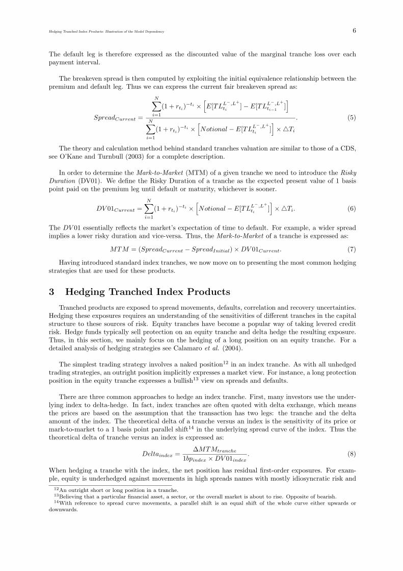
The default leg is therefore expressed as the discounted value of the marginal tranche loss over eachpayment interval.

The breakeven spread is then computed by exploiting the initial equivalence relationship between thepremium and default leg. Thus we can express the current fair breakeven spread as:

SpreadCurrent =

N∑

i=1

(1 + rti)−ti ×

[

E[TLL−,L+

ti] − E[TLL−,L+

ti−1]]

N∑

i=1

(1 + rti)−ti ×

[


ti]]

×Ti

. (5)

The theory and calculation method behind standard tranches valuation are similar to those of a CDS,see O’Kane and Turnbull (2003) for a complete description.

In order to determine the Mark-to-Market (MTM) of a given tranche we need to introduce the Risky

Duration (DV01). We define the Risky Duration of a tranche as the expected present value of 1 basispoint paid on the premium leg until default or maturity, whichever is sooner.

DV 01Current =

N∑

i=1

(1 + rti)−ti ×

[


ti]]

×Ti. (6)

The DV 01 essentially reflects the market’s expectation of time to default. For example, a wider spreadimplies a lower risky duration and vice-versa. Thus, the Mark-to-Market of a tranche is expressed as:

MTM = (SpreadCurrent − SpreadInitial) × DV 01Current. (7)

Having introduced standard index tranches, we now move on to presenting the most common hedgingstrategies that are used for these products.

3 Hedging Tranched Index Products

Tranched products are exposed to spread movements, defaults, correlation and recovery uncertainties.Hedging these exposures requires an understanding of the sensitivities of different tranches in the capitalstructure to these sources of risk. Equity tranches have become a popular way of taking levered creditrisk. Hedge funds typically sell protection on an equity tranche and delta hedge the resulting exposure.Thus, in this section, we mainly focus on the hedging of a long position on an equity tranche. For adetailed analysis of hedging strategies see Calamaro et al. (2004).

The simplest trading strategy involves a naked position12 in an index tranche. As with all unhedgedtrading strategies, an outright position implicitly expresses a market view. For instance, a long protectionposition in the equity tranche expresses a bullish13 view on spreads and defaults.

There are three common approaches to hedge an index tranche. First, many investors use the under-lying index to delta-hedge. In fact, index tranches are often quoted with delta exchange, which meansthe prices are based on the assumption that the transaction has two legs: the tranche and the deltaamount of the index. The theoretical delta of a tranche versus an index is the sensitivity of its price ormark-to-market to a 1 basis point parallel shift14 in the underlying spread curve of the index. Thus thetheoretical delta of tranche versus an index is expressed as:

Deltaindex =∆MTMtranche

1bpindex × DV 01index. (8)

When hedging a tranche with the index, the net position has residual first-order exposures. For exam-ple, equity is underhedged against movements in high spreads names with mostly idiosyncratic risk and

12An outright short or long position in a tranche.13Believing that a particular financial asset, a sector, or the overall market is about to rise. Opposite of bearish.14With reference to spread curve movements, a parallel shift is an equal shift of the whole curve either upwards or

downwards.


overhedged against low spread names with mostly systemic risk.

Second, investors can use single name CDS to hedge their position. The theoretical delta of a trancheversus an individual credit spread is the sensitivity of its price or mark-to-market to a 1 basis pointparallel shift in the underlying spread curve of the single name CDS. Thus the theoretical delta of atranche versus a single name CDS is expressed as:

DeltaCDS =∆MTMtranche

1bpCDS × DV 01CDS. (9)

There are two major determinants of single name deltas: spread and correlation. Higher spread nameshave a higher implied default probability, and thus are likely to have more impact on the junior tranches.The opposite is true for low spread names, which are more important to senior tranches. The seconddeterminant of delta is correlation. On the first hand, credits that are more correlated to the market areless important to the equity tranche. On the other hand, credits that are uncorrelated to the market asa whole represent an idiosyncratic risk and have the potential to hurt the equity tranche because theycan widen materially or even default without a corresponding effect across the market. The delta of theequity tranche to these credits is high.

Third, the most common trade over the past two years has been to take a long position in the equitytranches, and hedge or short the first mezzanine tranche. Investors delta hedge with other tranches ratherthan an index to increase the carry. The theoretical hedge ratio between two tranches can be expressedas:

HedgeRatio1,2 =∆MTMtranche1

1bpindex × DV 01index/

∆MTMtranche2

1bpindex × DV 01index. (10)

This is the ratio between the sensitivity of each tranche mark-to-market to a 1 basis point parallel shiftin the underlying spread curve of the index. In reality, the hedge ratio is commonly calculated usinga proportional shift of 5 or 10 basis points in the underlying spread curve of the index. The investorreceives more premium income by hedging with a leveraged product in exchange for assuming the riskthat the market may perform differently from model expectations. As long as the mezzanine tranchemoves in line with the model expectations, or as long as correlations between the equity and mezzaninetranches remain constant, the delta hedge works fine, and the investor pockets the income differential. If,however, mezzanine and equity tranches move differently than the assumed hedge ratio, the hedge fundcan lose on both sides of the trade. In fact, correlation has changed and tranche levels are not movingas models had predicted. A large market shock reveals that the assumptions underlying the models mayhave been inaccurate not only in size, but in sign.

As mentioned in Gibson (2004), the dynamic hedging of index tranches presents dealers with fourchallenges. First, the dealer must calculate the hedge positions (deltas or hedge ratios) of the index orgiven CDS in the reference index portfolio or other tranches. These deltas or hedge ratios are model-dependent, thus index tranches leave dealers with model risk. Second, the value of a index tranchedepends on the correlation assumption that is used to price and hedge it. Since default correlation isunobservable, a dealer is exposed to the risk that his correlation assumption is wrong (”correlation risk”).Third, as deltas change over time and the dealer dynamically adjusts his hedges, he is exposed to liquidityrisk. The credit default swap market may not have enough liquidity for the dealer to adjust its hedge asdesired without incurring high trading costs. Fourth, a dealer prefers to be hedged against both smallmoves in credit spreads (spread risk) and unexpected defaults (jump-to-default risk). Hedging againstboth risks adds complexity.

In the two next Sections we focus on the first two risks previously mentioned, the model risk and thecorrelation risk. We exhibit their implications by comparing empirical results versus historical data.


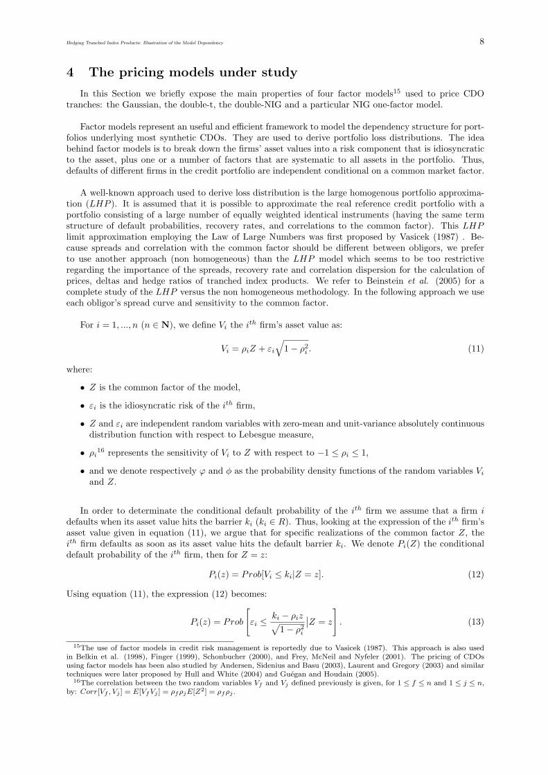
4 The pricing models under study

In this Section we briefly expose the main properties of four factor models15 used to price CDOtranches: the Gaussian, the double-t, the double-NIG and a particular NIG one-factor model.

Factor models represent an useful and efficient framework to model the dependency structure for port-folios underlying most synthetic CDOs. They are used to derive portfolio loss distributions. The ideabehind factor models is to break down the firms’ asset values into a risk component that is idiosyncraticto the asset, plus one or a number of factors that are systematic to all assets in the portfolio. Thus,defaults of different firms in the credit portfolio are independent conditional on a common market factor.

A well-known approach used to derive loss distribution is the large homogenous portfolio approxima-tion (LHP ). It is assumed that it is possible to approximate the real reference credit portfolio with aportfolio consisting of a large number of equally weighted identical instruments (having the same termstructure of default probabilities, recovery rates, and correlations to the common factor). This LHPlimit approximation employing the Law of Large Numbers was first proposed by Vasicek (1987) . Be-cause spreads and correlation with the common factor should be different between obligors, we preferto use another approach (non homogeneous) than the LHP model which seems to be too restrictiveregarding the importance of the spreads, recovery rate and correlation dispersion for the calculation ofprices, deltas and hedge ratios of tranched index products. We refer to Beinstein et al. (2005) for acomplete study of the LHP versus the non homogeneous methodology. In the following approach we useeach obligor’s spread curve and sensitivity to the common factor.

For i = 1, ..., n (n ∈ N), we define Vi the ith firm’s asset value as:

Vi = ρiZ + εi

√

1 − ρ2i . (11)

where:

• Z is the common factor of the model,

• εi is the idiosyncratic risk of the ith firm,

• Z and εi are independent random variables with zero-mean and unit-variance absolutely continuousdistribution function with respect to Lebesgue measure,

• ρi16 represents the sensitivity of Vi to Z with respect to −1 ≤ ρi ≤ 1,

• and we denote respectively ϕ and φ as the probability density functions of the random variables Vi

and Z.

In order to determinate the conditional default probability of the ith firm we assume that a firm idefaults when its asset value hits the barrier ki (ki ∈ R). Thus, looking at the expression of the ith firm’sasset value given in equation (11), we argue that for specific realizations of the common factor Z, theith firm defaults as soon as its asset value hits the default barrier ki. We denote Pi(Z) the conditionaldefault probability of the ith firm, then for Z = z:

Pi(z) = Prob[Vi ≤ ki|Z = z]. (12)

Using equation (11), the expression (12) becomes:

Pi(z) = Prob

[

εi ≤ki − ρiz√

1 − ρ2i

∣

∣Z = z

]

. (13)

15The use of factor models in credit risk management is reportedly due to Vasicek (1987). This approach is also usedin Belkin et al. (1998), Finger (1999), Schonbucher (2000), and Frey, McNeil and Nyfeler (2001). The pricing of CDOsusing factor models has been also studied by Andersen, Sidenius and Basu (2003), Laurent and Gregory (2003) and similartechniques were later proposed by Hull and White (2004) and Guegan and Houdain (2005).

16The correlation between the two random variables Vf and Vj defined previously is given, for 1 ≤ f ≤ n and 1 ≤ j ≤ n,by: Corr[Vf , Vj ] = E[Vf Vj ] = ρf ρjE[Z2] = ρf ρj .


We denote Cεithe cumulative distribution for the random variable εi, then the probability given in (13)

for Z = z and for i = 1, ..., n is equal to:

Pi(z) = Cεi

[

ki − ρiz√

1 − ρ2i

]

. (14)

In order to determine the real value of the default barrier ki for each firm i, we denote Qi the unconditionaldefault probability of the ith firm. Qi is recovered from CDS market data using an intensity-basedmodel17 or by bootstrapping the CDS spread curve of the underlying firm. The default barrier ki is equalto ϕ−1(Qi). When it is impossible to determine the distribution of the random variable Vi then we needto use the following approach. By definition we have:

Qi = Prob[Vi ≤ ki] = E[Pi(Z)]. (15)

If φ represents the density function of the random variable Z, then:

E[Pi(Z)] =

∫ +∞

−∞

Pi(z)φ(z)dz, (16)

which implies that:

Qi =

∫ +∞

−∞

Cεi

[

ki − ρiz√

1 − ρ2i

]

φ(z)dz. (17)

Now, to determine the default barrier of the ith firm we need to solve in ki the Equation 17.

Under such modeling assumptions, it is possible to determine the underlying portfolio loss distributionby numerically computing the inverse Fast Fourier Transform18 or some other inversion method. Becauseof computation complexity of the Fast Fourier Transform, we present in this paper an alternative basedon a recursive methodology introduced by Galiani et al. (2004).

We define Ωkn,z as the conditional aggregate probability of having k defaults in an n-credit portfolio.

For a one-credit portfolio and a specific realisation of Z, the probability Ω11,z of having one default equals

P1(z) whereas the probability Ω01,z of having no default is equal to 1 − P1(z). Regarding a two-credit

portfolio and given the conditional independence of the defaults, the probability Ω02,z of having no default

is equal to (1− P1(z))(1− P2(z)) and the probability of having two defaults Ω22,z is equal to P1(z)P2(z).

The probability Ω12,z of having only one default is less intuitive and is equal to Ω1

1,z(1−P1(z))+Ω01,zP2(z).

This recursive approach can be extend to any n-credit portfolio using the following recursive algorithm:

Ωkn+1,z = Ωk

n,z(1 − Pn+1(z)) + Ωk−1n,z Pn+1(z). (18)

The unconditional distribution is given by:

Ωkn+1 =

∫ +∞

−∞

Ωkn+1,zφ(z)dz. (19)

Using the previously described properties we can derived a loss distribution for each payment date.Now we are going to describe different approaches that have been generated to fit the observed marketprices of index tranches using factor models.

4.1 The Gaussian one-factor model

The Gaussian one-factor model has become the established way of pricing tranched index products.The new availability of relatively liquid market levels has led to the price quotes of the tranches in terms

17The first published intensity model appears to be Jarrow and Turnbull (1995). Subsequent research includes Duffie andHuang (1996), Jarrow, Lando and Turnbull (1997) and Duffie, Singleton (1997a, 1997b) and Schonbucher and Schubert(2001). The fundamental idea of the intensity-based model framework is to model the default probability as the first jumpof a Poisson process.

18See Press et al. (1992).


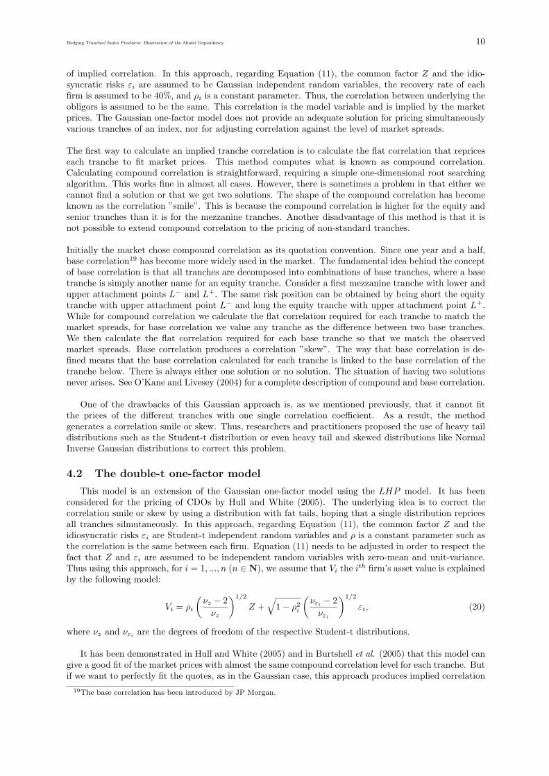
of implied correlation. In this approach, regarding Equation (11), the common factor Z and the idio-syncratic risks εi are assumed to be Gaussian independent random variables, the recovery rate of eachfirm is assumed to be 40%, and ρi is a constant parameter. Thus, the correlation between underlying theobligors is assumed to be the same. This correlation is the model variable and is implied by the marketprices. The Gaussian one-factor model does not provide an adequate solution for pricing simultaneouslyvarious tranches of an index, nor for adjusting correlation against the level of market spreads.

The first way to calculate an implied tranche correlation is to calculate the flat correlation that repriceseach tranche to fit market prices. This method computes what is known as compound correlation.Calculating compound correlation is straightforward, requiring a simple one-dimensional root searchingalgorithm. This works fine in almost all cases. However, there is sometimes a problem in that either wecannot find a solution or that we get two solutions. The shape of the compound correlation has becomeknown as the correlation ”smile”. This is because the compound correlation is higher for the equity andsenior tranches than it is for the mezzanine tranches. Another disadvantage of this method is that it isnot possible to extend compound correlation to the pricing of non-standard tranches.

Initially the market chose compound correlation as its quotation convention. Since one year and a half,base correlation19 has become more widely used in the market. The fundamental idea behind the conceptof base correlation is that all tranches are decomposed into combinations of base tranches, where a basetranche is simply another name for an equity tranche. Consider a first mezzanine tranche with lower andupper attachment points L− and L+. The same risk position can be obtained by being short the equitytranche with upper attachment point L− and long the equity tranche with upper attachment point L+.While for compound correlation we calculate the flat correlation required for each tranche to match themarket spreads, for base correlation we value any tranche as the difference between two base tranches.We then calculate the flat correlation required for each base tranche so that we match the observedmarket spreads. Base correlation produces a correlation ”skew”. The way that base correlation is de-fined means that the base correlation calculated for each tranche is linked to the base correlation of thetranche below. There is always either one solution or no solution. The situation of having two solutionsnever arises. See O’Kane and Livesey (2004) for a complete description of compound and base correlation.

One of the drawbacks of this Gaussian approach is, as we mentioned previously, that it cannot fitthe prices of the different tranches with one single correlation coefficient. As a result, the methodgenerates a correlation smile or skew. Thus, researchers and practitioners proposed the use of heavy taildistributions such as the Student-t distribution or even heavy tail and skewed distributions like NormalInverse Gaussian distributions to correct this problem.

4.2 The double-t one-factor model

This model is an extension of the Gaussian one-factor model using the LHP model. It has beenconsidered for the pricing of CDOs by Hull and White (2005). The underlying idea is to correct thecorrelation smile or skew by using a distribution with fat tails, hoping that a single distribution repricesall tranches silmutaneously. In this approach, regarding Equation (11), the common factor Z and theidiosyncratic risks εi are Student-t independent random variables and ρ is a constant parameter such asthe correlation is the same between each firm. Equation (11) needs to be adjusted in order to respect thefact that Z and εi are assumed to be independent random variables with zero-mean and unit-variance.Thus using this approach, for i = 1, ..., n (n ∈ N), we assume that Vi the ith firm’s asset value is explainedby the following model:

Vi = ρi

(

νz − 2

νz

)1/2

Z +√

1 − ρ2i

(

νεi− 2

νεi

)1/2

εi, (20)

where νz and νεiare the degrees of freedom of the respective Student-t distributions.

It has been demonstrated in Hull and White (2005) and in Burtshell et al. (2005) that this model cangive a good fit of the market prices with almost the same compound correlation level for each tranche. Butif we want to perfectly fit the quotes, as in the Gaussian case, this approach produces implied correlation

19The base correlation has been introduced by JP Morgan.


because the correlation parameter ρ becomes one of the three variables of the model. The two othervariables are the degrees of freedom of the Student-t distributions of Z and of the εi. In this paper, wehave implemented this model using the non homogeneous methodology previously described in Section 4and constant 40% recovery rate.

4.3 The NIG one-factor model with historical correlations

This model has been introduced by Guegan and Houdain (2005). The underlying idea of this approachis to use the price quotes of the tranches available in the market to determine the implied NIG-distributionof the common factor for a given input correlation level. In the market standard methodology, the dis-tributions used in the factor model are fixed and the implied correlation of a tranche is calculated underthese assumptions. We have used an opposite approach: we fix the correlation of the portfolio and thedistribution of the idiosyncratic risk of each firm and then we determine the implied NIG-distribution ofthe common factor in the model.

The Normal Inverse Gaussian20 distribution has the remarkable property of being able to representstochastic phenomena that have heavy tails and/or are strongly skewed. This distribution is characterizedby 4 parameters (α, β, µ, δ). The parameter α is related to steepness, β to symmetry, and µ and δrespectively to location and scale. The NIG(α, β, µ, δ) Probability Density Function is given by:

NIG(x;α, β, µ, δ) = a(α, β, µ, δ)q

(

x − µ

δ

)−1

K1

(

δαq

(

x − µ

δ

))

eβx, (21)

with:

q(x) =√

1 + x2, (22)

and,

a(α, β, µ, δ) = π−1α exp(δ√

α2 − β2 − βµ). (23)

Here K1 is a modified Bessel function of the third kind with index 1 defined as:

K1(x) = x

∫ ∞

1

exp(−xt)√

t2 − 1dt. (24)

The necessary conditions for a non-degenerated density are δ > 0, α > 0 and |β|α < 1. The Moment

Generating Function of a NIG-distributed random variable X is equal to:

MX(u) = exp(uµ + δ(√

α2 − β2 −√

α2 − (β + u)2)). (25)

From equation (25) we can derive:

E[X] = µ + δ

(

β

γ

)

, (26)

V ar[X] = δ

(

α2

γ3

)

, (27)

Skew[X] = 3

(

β

α

)(

1

(δγ)1/2

)

, (28)

Kurt[X] = 3

(

1 + 4

(

β

α

)2)

(

1

(δγ)

)

, (29)

20The NIG distribution was introduced to investigate the properties of the returns from financial markets by Barndorff-Nielsen (1997). Since then, applications in finance have been reported in several papers, both for the conditional distributionof a GARCH model (Jensen and Lunde (2001); Forsberg and Bollerslev (2002); Venter and de Jongh (2002)) and for theunconditional distribution (Prause (1997); Rydberg (1997); Bolviken and Benth (2000); Lillestol (1998-2000-2001-2002);Venter and de Jongh (2002); Guegan and Houdain (2005)).


with γ =√

α2 − β2. From equations (28) and (29), and since |β|α < 1, we obtain some properties of the

kurtosis and the skewness:Kurt[X] > 3, (30)

and,

3 +5

3(Skew[X])2 < Kurt[X]. (31)

To respect the fact that Z and εi are independent random variables with zero-mean and unit-variancethe parameters α, β, µ and δ need to be scaled.

One of the main properties of the NIG distribution class are the scaling property:

X ∼ NIG(α, β, µ, δ) ⇒ ςX ∼ NIG(α

ς,β

ς, ςµ, ςδ). (32)

Another important property of the Normal Inverse Gaussian distribution is its behavior under convo-lutions. Indeed, if X1 and X2 are independent and distributed respectively as NIG(α, β, µ1, δ1) andNIG(α, β, µ2, δ2). Then X1 + X2 is a NIG(α, β, µ1 + µ2, δ1 + δ2).

Using the previously described properties of the NIG distribution it is possible to fit the market quoteof each tranche with the same correlation structure. In the real world the asset value of each firm wouldhave a different correlation with the asset value of each other firm in the portfolio. In this methodologythe correlation between the underlying assets of the portfolio becomes an input. In this paper, we esti-mate the pairwise correlations using the methodology proposed by Andersen, Sidinius and Basu (2003)and the correction proposed by Jackel (2005) based on equity returns correlation 21 and Frobenius normto determine the factor loadings. We also use the recovery rates provided by the rating agencies. Formore details please refer to Guegan and Houdain (2005).

It has been demonstrated that this model seems to be the best alternative if we want to price a nonstandard or bespoke tranche CDO. Thus it would be interesting to see if the model should be a goodalternative to hedge standard tranche index products.

4.4 The double-NIG one-factor model

The double-NIG one-factor model is also an extension of the Gaussian one-factor model using the LHPmodel. It has been considered for the pricing of CDOs by Kalemanova et al. (2005). The underlying ideais to correct the correlation smile or skew by using a heavy tail and skewed distribution. In this approach,regarding Equation (11), the common factor Z and the idiosyncratic risks εi are Normal Inverse Gaussianindependent random variables and ρ is a constant parameter such as the correlation is the same betweeneach firm. As in the Double-t model, if we want to perfectly fit the quotes, this approach produces impliedcorrelation.

The underlying idea of the double-NIG one-factor model is to benefit from the two last describedproperties of the NIG distribution and then to easily compute the default barrier of each firm ki =ϕ−1(Qi). In this paper, we have implemented this model using the non homogeneous methodologypreviously described in Section 4 and constant 40% recovery rate.

21On a one year period.


4.5 Summary of the studied models

We can summarize the specificities of each model as fallow:

LHP Non Homogeneous Non HomogeneousAssumption (Gaussian, Student-t, NIG) (Gaussian, Student-t, NIG) (NIG)

with Base correlation with Historical correlation

Index portfolio Infinite obligors Actual number of obligors Actual number of obligorsSpread curves shape Flat curves Full curves Full curvesUnderlying spreads Single Index spread Individual obligor spreads Individual obligor spreads

Correlation structure Identical pairwise correlation Identical pairwise correlation Historical pairwise correlationRecovery rate 40% 40% Rating agencies recovery rates

Table 1: Summary of the different models.

In the next section we compare the hedging capabilities of these different non homogeneous factormodels.

5 Models outputs versus historical data

It has been demonstrated in the literature that the previously described models can fit the tranches’market quotes. Thus, in this section we are going to study their differences in terms of hedging capabilities.In order to compare our results with historical data, we will study the behavior of the iTraxx series 3and 4 and its 0 − 3% and 3 − 6% underlying tranches from the 21th of March 2005 to the 20th of March2006. The idea is to offset the Mark-to-Market risk of a long position in the equity tranche with a wellchosen short position in the first mezzanine tranche. For simplicity we assume that tranches are tradedwithout the index delta exchange and that the equity piece is traded in running spread without upfrontpayment. For the equity tranche, running spread and upfront are linked by the following relation:

Spreadrunning =Upfront

DV 01tranche× 100 + 500. (33)

In Figure 3, we illustrate the daily MTM variations of the two less subordinated iTraxx underlyingtranches from the 20th of March 2005 to the 20th of March 2006. The index tranche market experienceda great deal of volatility in the second week of May 2005, after S&P downgraded General Motors andFord to junk status which lead to an extensive spread widening in the CDS indices. These two NorthAmerican companies were not part of the iTraxx so we have been, during this period, the witnesses ofa very important contagion effect between the North American tranche market and the European one.Some practitioners and researchers have tried and are currently trying to explain this phenomena or moreexactly this major crisis. One of the principal explanations is that just after these downgrades, hedgefunds began to reduce leverage in the index tranche market and reversed the existing behavior between thetranches’ returns. By the way, for the purpose of this paper we just have to keep in mind that during May2005 the behavior of the European tranches has changed but not as much as the North American tranches.

Regarding the studied strategy, the underlying idea of hedging the equity tranche with the first mez-zanine one is to find the best hedge ratio between these two tranches. Figures 3 illustrates the fact thatthe sensitivity of the tranches is quite different regarding the maturity and the well known fact that fora 10 year maturity the first mezzanine tranche behaves more like an equity piece. This behavior shouldbe explained by the fact that the expected loss of the iTraxx 5Y is arround 1.7% on the studied periodbut arround 5.7% for the iTraxx 10Y which means that the first mezzanine tranche with an attachmentpoint at 3% is more likely to be eaten for a 10 years maturity.

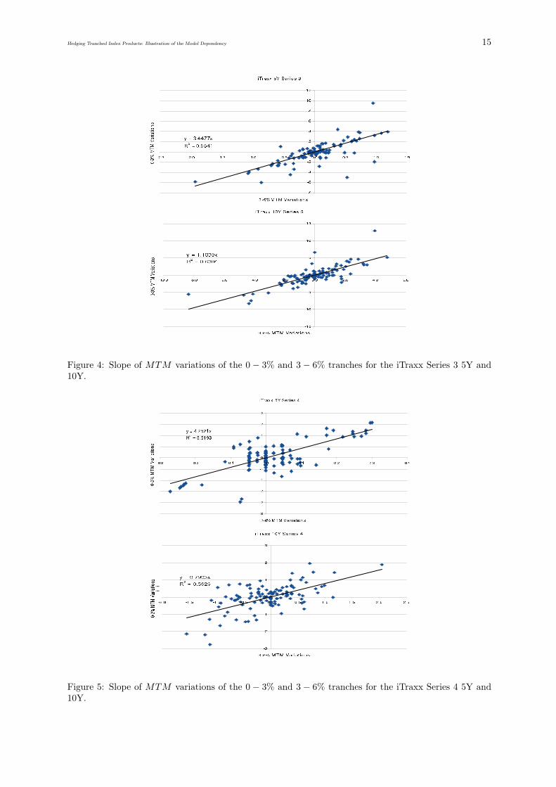
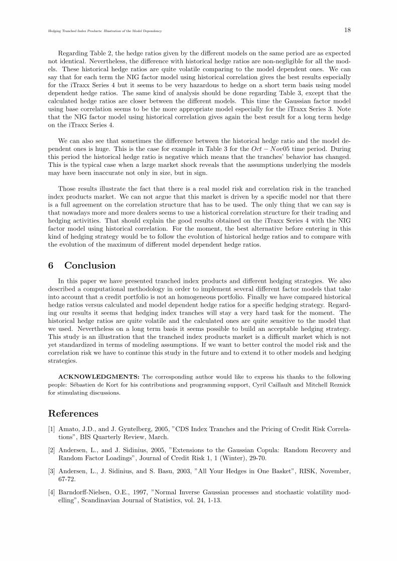
Figures 4 and 5 present the scatter plots of the daily MTM variations of the 0 − 3% and 3 − 6%tranches for a 5 and 10 years maturity from the 21th of March 2005 to the 20th of September 2005 forthe iTraxx Series 3 and from the 21th of September 2005 to the 20th of March 2006 for the iTraxx Series4. We can see some extreme events in the iTraxx Series 3 due to the May 2005 crisis. We can see alsothat the historical hedge ratios are easily observable but should be quite volatile in time. Thus, in Table2 and 3 we present the historical hedge ratios between the equity and the first mezzanine tranches of theiTraxx for a 5 and 10 years maturity on monthly, quarterly and semestrial time intervals which should


Figure 3: Evolution of the tranches’ Mark-to-Market since March 2005.

be respectively analyzed as short term, mean term and long term hedging strategy. These hedge ratiosare the slope in a regression of daily MTM variations in the tranches. We compare this historical resultswith the ratios given by the several models previously described in Section 4. In columns 4, 6, 8 and 10 wehave calculated the absolute difference between historical hedge ratios and model dependent hedge ratios.For each time interval we present the average of these absolute differences. Note that for the calculationof the hedge ratios we used Equation 10 with a 5 basis points proportional shift in the underlying spreadcurve of the iTraxx. We chose a 5 basis points proportional shift because it gives better results than aparallel or another proportional shift for all the models comparing to historical hedge ratios. It is in linewith the market that the curves may be perturbed proportionally, with wider spread names moving morethan tight spread ones, to reflect better typical spread moves.


Figure 4: Slope of MTM variations of the 0 − 3% and 3 − 6% tranches for the iTraxx Series 3 5Y and10Y.

Figure 5: Slope of MTM variations of the 0 − 3% and 3 − 6% tranches for the iTraxx Series 4 5Y and10Y.

Hedgin

gTra

nch

ed

Index

Pro

ducts:

Illustra

tion

ofth

eM

odelD

ependency

16

Market Base Correlation Historical CorrelationPeriod Slope Gaussian Abs Diff Double-t Abs Diff Double-NIG Abs Diff NIG Abs Diff

Mar-Apr05 3.38 4.38 1.00 4.09 0.71 4.19 0.81 3.89 0.51

Apr-May05 3.62 4.45 0.83 4.16 0.54 4.26 0.64 3.95 0.33

May-Jun05 3.77 4.38 0.61 4.10 0.33 4.20 0.43 3.89 0.12

Jun-Jul05 4.76 4.59 0.17 4.29 0.47 4.40 0.36 4.08 0.68Jul-Aug05 2.29 4.49 2.20 4.20 1.91 4.30 2.01 3.99 1.70

Aug-Sep05 3.47 4.63 1.16 4.33 0.86 4.44 0.97 4.11 0.64

Sep-Oct05 5.07 4.77 0.30 4.46 0.82 4.57 0.5 4.24 0.83Oct-Nov05 3.54 4.75 1.21 4.44 0.90 4.55 1.01 4.22 0.68

Nov-Dec05 4.06 4.80 0.74 4.48 0.42 4.60 0.54 4.26 0.20

Dec-Jan06 5.26 4.82 0.44 4.51 0.75 4.62 0.64 4.28 0.98Jan-Feb06 3.80 4.73 0.93 4.42 0.62 4.53 0.73 4.20 0.40

Feb-Mar06 3.80 4.80 1.65 4.40 1.25 4.50 1.35 4.18 1.03

Average Abs Diff 0.94 0.78 0.83 0.68

Mar-Jun05 3.56 4.38 0.82 4.09 0.53 4.19 0.63 3.89 0.33

Jun-Sep05 3.69 4.59 0.90 4.29 0.60 4.40 0.71 4.08 0.39

Sep-Dec05 4.48 4.77 0.29 4.46 0.02 4.57 0.09 4.24 0.24Dec-Mar06 4.08 4.82 0.74 4.51 0.43 4.62 0.54 4.28 0.20

Average Abs Diff 0.69 0.40 0.49 0.29

iTraxx3 3.56 4.38 0.82 4.09 0.53 4.19 0.63 3.89 0.33

iTraxx4 4.32 4.77 0.45 4.46 0.14 4.57 0.25 4.24 0.08

Average Abs Diff 0.64 0.34 0.44 0.21

Table 2: Hedge Ratio calculations vs historical Hedge Ratio for the iTraxx 5Y.

Hedgin

gTra

nch

ed

Index

Pro

ducts:

Illustra

tion

ofth

eM

odelD

ependency

17

Market Base Correlation Historical CorrelationPeriod Slope Gaussian Abs Diff Double-t Abs Diff Double-NIG Abs Diff NIG Abs Diff

Mar-Apr05 1.51 1.14 0.37 1.05 0.46 0.99 0.52 0.81 0.70Apr-May05 1.26 1.06 0.20 0.97 0.29 0.92 0.34 0.79 0.47May-Jun05 0.73 1.02 0.29 0.94 0.21 0.88 0.15 0.83 0.10

Jun-Jul05 0.91 0.94 0.03 0.87 0.04 0.82 0.09 0.80 0.11Jul-Aug05 0.33 0.92 0.59 0.85 0.52 0.80 0.47 0.82 0.49Aug-Sep05 1.03 0.95 0.08 0.87 0.16 0.82 0.21 0.83 0.20Sep-Oct05 0.86 0.90 0.04 1.05 0.19 0.98 0.12 0.74 0.12Oct-Nov05 -0.18 1.10 1.28 1.01 1.19 0.95 1.13 0.69 0.87

Nov-Dec05 0.65 1.08 0.43 0.99 0.34 0.93 0.28 0.68 0.03

Dec-Jan06 1.29 1.12 0.17 1.03 0.26 0.97 0.32 0.71 0.58Jan-Feb06 1.02 1.11 0.09 1.02 0.00 0.96 0.06 0.68 0.34Feb-Mar06 0.22 0.91 0.69 1.10 0.88 0.98 0.76 0.70 0.48

Average Abs Diff 0.36 0.38 0.37 0.37

Mar-Jun05 1.26 1.14 0.12 1.05 0.21 0.99 0.27 0.81 0.45Jun-Sep05 0.85 0.94 0.09 0.87 0.02 0.82 0.03 0.80 0.05Sep-Dec05 0.61 0.98 0.29 1.05 0.44 0.98 0.37 0.74 0.13Dec-Mar06 0.91 1.12 0.21 1.03 0.12 0.97 0.06 0.71 0.20

Average Abs Diff 0.18 0.20 0.18 0.21

iTraxx3 1.18 1.14 0.04 1.05 0.13 0.99 0.19 0.81 0.37iTraxx4 0.80 0.90 0.10 1.05 0.25 0.98 0.18 0.74 0.06

Average Abs Diff 0.07 0.19 0.19 0.22

Table 3: Hedge Ratio calculations vs historical Hedge Ratio for the iTraxx 10Y.


Regarding Table 2, the hedge ratios given by the different models on the same period are as expectednot identical. Nevertheless, the difference with historical hedge ratios are non-negligible for all the mod-els. These historical hedge ratios are quite volatile comparing to the model dependent ones. We cansay that for each term the NIG factor model using historical correlation gives the best results especiallyfor the iTraxx Series 4 but it seems to be very hazardous to hedge on a short term basis using modeldependent hedge ratios. The same kind of analysis should be done regarding Table 3, except that thecalculated hedge ratios are closer between the different models. This time the Gaussian factor modelusing base correlation seems to be the more appropriate model especially for the iTraxx Series 3. Notethat the NIG factor model using historical correlation gives again the best result for a long term hedgeon the iTraxx Series 4.

We can also see that sometimes the difference between the historical hedge ratio and the model de-pendent ones is huge. This is the case for example in Table 3 for the Oct − Nov05 time period. Duringthis period the historical hedge ratio is negative which means that the tranches’ behavior has changed.This is the typical case when a large market shock reveals that the assumptions underlying the modelsmay have been inaccurate not only in size, but in sign.

Those results illustrate the fact that there is a real model risk and correlation risk in the tranchedindex products market. We can not argue that this market is driven by a specific model nor that thereis a full agreement on the correlation structure that has to be used. The only thing that we can say isthat nowadays more and more dealers seems to use a historical correlation structure for their trading andhedging activities. That should explain the good results obtained on the iTraxx Series 4 with the NIGfactor model using historical correlation. For the moment, the best alternative before entering in thiskind of hedging strategy would be to follow the evolution of historical hedge ratios and to compare withthe evolution of the maximum of different model dependent hedge ratios.

6 Conclusion

In this paper we have presented tranched index products and different hedging strategies. We alsodescribed a computational methodology in order to implement several different factor models that takeinto account that a credit portfolio is not an homogeneous portfolio. Finally we have compared historicalhedge ratios versus calculated and model dependent hedge ratios for a specific hedging strategy. Regard-ing our results it seems that hedging index tranches will stay a very hard task for the moment. Thehistorical hedge ratios are quite volatile and the calculated ones are quite sensitive to the model thatwe used. Nevertheless on a long term basis it seems possible to build an acceptable hedging strategy.This study is an illustration that the tranched index products market is a difficult market which is notyet standardized in terms of modeling assumptions. If we want to better control the model risk and thecorrelation risk we have to continue this study in the future and to extend it to other models and hedgingstrategies.

ACKNOWLEDGMENTS: The corresponding author would like to express his thanks to the following

people: Sebastien de Kort for his contributions and programming support, Cyril Caillault and Mitchell Reznick

for stimulating discussions.

References

[1] Amato, J.D., and J. Gyntelberg, 2005, ”CDS Index Tranches and the Pricing of Credit Risk Correla-tions”, BIS Quarterly Review, March.

[2] Andersen, L., and J. Sidinius, 2005, ”Extensions to the Gaussian Copula: Random Recovery andRandom Factor Loadings”, Journal of Credit Risk 1, 1 (Winter), 29-70.

[3] Andersen, L., J. Sidinius, and S. Basu, 2003, ”All Your Hedges in One Basket”, RISK, November,67-72.

[4] Barndorff-Nielsen, O.E., 1997, ”Normal Inverse Gaussian processes and stochastic volatility mod-elling”, Scandinavian Journal of Statistics, vol. 24, 1-13.


[5] Belkin, B., S. Suchover, and L. Forest, 1998, ”A one-parameter representation of credit risk andtransition matrices”, Credit Metrics Monitor, 1(3), 46-56.

[6] Beinstein, E., A. Sbityakov, P. Allen, and D. Dirk, 2005, ”Enhancing our framework for index trancheanalysis”, Credit Derivatives Research, JPMorgan.

[7] Burtschell, X., J. Gregory, and J-P. Laurent, 2005, ”A comparative analysis of CDO pricing models”,www.defaultrisk.com.

[8] Burtschell, X., J. Gregory, and J-P. Laurent, 2005, ”Beyond the Gaussian Copula: Stochastic andLocal Correlation”, www.defaultrisk.com.

[9] Calamaro, J-P., T. Nassar, K. Thakkar, and J. Tierney, 2004, ”Trading Index Tranche Products: TheFirst Steps”, Quantitative Credit Strategy, Deutsche Bank.

[10] Derman, E., 2004, ”My Life As A Quant: Reflections on Physics and Finance”, John Wiley & Sons.

[11] Duffie, D., and M. Huang, 1996, ”Swap Rates and Credit Quality”, Journal of Finance, 51(2),921-949.

[12] Duffie, D. and K. Singleton, 1997, ”Modeling term structures of defaultable bonds”, Review ofFinancial Studies, 12(4), 687-720.

[13] Duffie, D. and K. Singleton, 1997, ”An Econometric Model of the Term Structure of Interest-RateSwap Yields”, Journal of Finance, 52(4), 1287-1321.

[14] Finger, C.C., 1999, ”Conditional approaches for credit metrics portfolio distributions”, Credit Met-rics Monitor, 2(1), 14-33.

[15] Forsberg, L., and T. Bollerslev, 2002, ”Bridging the Gap Between the Distribution of Realized(ECU) Volatility and ARCH modeling (of the EURO): The GARCH-NIG model”, Journal of AppliedEconometrics, Vol. 17, No. 5, 535-548.

[16] Frey, R., A. McNeil, and N. Nyfeler, 2001, ”Copulas and Credit Models”, RISK, October, 111-114.

[17] Jensen, M.B., and A. Lunde, 2001, ”The NIG-S&ARCH model: a fat-tailed, stochastic, and autore-gressive conditional heteroskedastic volatility model”, Econometrics Journal, Royal Economic Society,vol. 4(2), 10.

[18] Galiani, S., 2004, ”Understanding the Risk of Synthetic CDOs”,http://www.federalreserve.gov/Pubs/FEDS/2004/200436/200436pap.pdf.

[19] Gibson, M.S., M. Shchetkovskiy and A. Kakodkar, 2004, ”Basket Default Swap Valuation”, CreditDerivatives, Merrill Lynch.

[20] Guegan, D., and J. Houdain, 2005, ”Collateralized Debt Obligations Pricing and Factor Models:A New Methodology Using Normal Inverse Gaussian Distributions”, www.defaultrisk.com/pp crdrv93.htm.

[21] Hull, J., and A. White, 2004, ”Valution of a CDO and an nth-to-default CDS without Monte Carlosimulation”, Working Paper, University of Toronto.

[22] Hull, J., and A. White, 2005, ”The Perfect Copula”, Working Paper, University of Toronto.

[23] Jackel, P., 2005, ”Splitting the core”, Working paper, http://www.jaeckel.org.

[24] Jarrow, R.A., and S.M. Turnbull, 1995, ”Pricing Derivatives on Financial Securities Subject to CreditRisk”, Journal of Finance, 50(1), 53-85.

[25] Jarrow, R., D. Lando, and S. Turnbull, 1997, ”A Markov model for the term structure of creditspreads”, Review of Financial Studies, 10(2), 481-523.

[26] Kalemanova, A., B. Schmid and R. Werner, 2005, ”The Normal inverse Gaussian distribution forsynthetic CDO”, working paper.


[27] Laurent, J-P. and J., Gregory, 2003, ”Basket Default Swaps, CDO’s and Factor Copulas”, WorkingPaper ISFA Actuarial School, University of Lyon and BNP-Paribas.

[28] Lillestol, J., 1998, ”Fat and skew? Can NIG cure? On the prospects of using the Normal inverseGaussian distribution in finance”, Discussion paper 1998/11, Department of Finance and ManagementScience, The Norwegian School of Economics and Business Administration.

[29] Lillestol, J., 2000, ”Risk analysis and the NIG distribution”, The Journal of Risk, 2, 41-56.

[30] Lillestol, J., 2001, ”Bayesian Estimation of NIG-parameters by Markov chain Monte Carlo Methods”,Discussion paper 2001/3, Department of Finance and Management Science, The Norwegian School ofEconomics and Business Administration.

[31] Lillestol, J., 2002, ”Some crude approximation, calibration and estimation procedures for NIG-variates”, Department of Finance and Management Science, The Norwegian School of Economics andBusiness Administration.

[32] O’Kane, D. and M. Livesey, 2004, ”Base Correlation Explained”, Fixed Income Quantitative CreditResearch, Lehman Brothers.

[33] Prause, K., 1997, ”Modelling financial data using generalized hyperbolic distributions”, FDMPreprint 48. University of Freiburg.

[34] Press, W.H., B.P. Flannery, S.A. Teukolsky, and W.T. Vetterling, 1992, ”Fast Fourier Transform”,Numerical Recipes in FORTRAN: The Art of Scientific Computing, 2nd ed. Cambridge, England:Cambridge University Press, Ch.12, 490-529.

[35] Rydberg, T., 1997, ”The normal inverse Gaussian Levy processes: simulation and approximation”,Commun. Statist.-Stochastic Models., 13(4), 887-910.

[36] Schonbucher, P.J., 2000, ”Factor models for portfolio credit risk”, Working Paper.

[37] Schonbucher, P.J., and D. Schubert, 2001, ”Copula-dependent default risk in intensity models”,Department of Statistics, Bonn University, Working Paper.

[38] Vasicek, O., 1987, ”The loan loss distribution”, Working Paper, KMV Corporation.

[39] Venter , J.H. and de Jongh, P.J., 2002, ”The effects on risk and volatility estimation when us-ing different innovation distributions in GARCH models”, Research Report FABWI-N-RA: 2002-98,Potchefstroom University for CHE.

[40] Venter , J.H. and de Jongh, P.J., 2002, ”Risk Estimation using the Normal Inverse Gaussian Distri-bution”, The Journal of Risk, Vol. 4, No. 2, 1-23.

[41] Walker, M.B., 2005, ”An Incomplete-Market Model for Collateralized Debt Obligations”,http://www.physics.utoronto.ca/qocmp/incompleteCDO.2005.10.05.pdf.

[42] Walker, M.B., 2005, ”CDO Models Towards the Next Generation: Incomplete Markets and TermStructure”, http://www.physics.utoronto.ca/ qocmp/nextGenDefaultrisk.pdf.

hedging tranched index products: illustration of the model

Documents