Distance function wavelets – Part I: Helmholtz and convection-diffusion

transforms and series

W. Chen

Simula Research Laboratory, P. O. Box. 134, 1325 Lysaker, Norway

E-mail: wenc@simula.no

(9 May 2002)

Summary

This report aims to present my research updates on distance function wavelets (DFW)

based on the fundamental solutions and general solutions of the Helmholtz, modified

Helmholtz, and convection-diffusion equations, which include the isotropic Helmholtz-

Fourier (HF) transform and series, the Helmholtz-Laplace (HL) transform, and the

anisotropic convection-diffusion wavelets and ridgelets. The latter is set to handle

discontinuous and track data problems. The edge effect of the HF series is addressed.

Alternative existence conditions for the DFW transforms are proposed and discussed. To

simplify and streamline the expression of the HF and HL transforms, a new dimension-

dependent function notation is introduced. The HF series is also used to evaluate the

analytical solutions of linear diffusion problems of arbitrary dimensionality and

geometry. The weakness of this report is lacking of rigorous mathematical analysis due to

the author’s limited mathematical knowledge.

Keywords: Helmholtz-Fourier transform and series, Helmholtz-Laplace transform,

distance function, radial basis function, distance function wavelet, ridgelets, Helmholtz

equation, modified Helmholtz equation, convection-diffusion equation, fundamental

solution, general solution, edge effect.

1

1. Introduction

This report is the first in series [1,2] about my latest advances on the distance function

wavelets (DFW) using the fundamental solution and general solution of partial

differential equations (PDEs). It is well known that the Helmholtz and modified

Helmholtz equations are of vital importance in many basic and applied fields. In

particular, it is worth pointing out that the omnipresent Fourier analysis and Laplace

transform have their origin from the solution of the 1D Helmholtz equations [3,4]. The

DFW’s based on the solutions of Helmholtz equations could be understood a

generalization of the formers via the distance variable instead of coordinate variables.

This report focuses on the Helmholtz-Fourier (HF) transform and series and the

Helmholtz-Laplace (HL) transform, respectively corresponding to the Helmholtz

equation and the modified Helmholtz equation. Serving as an illustration of their

applications, the HF series is employed to get the analytical solutions of the linear

diffusion equations of arbitrary dimensionality and geometry [5]. Furthermore, the

anisotropic DFW using the solution of the convection-diffusion equation is proposed to

handle discontinuous and track data problems. The underlying connection between such

anisotropic DFW and ridgelets is also discussed. The present wavelet transform and

series differ from the standard wavelets in that they use the solution of PDEs as do the

Fourier and Laplace analyses. The DFW’s could be of widespread use in handling

multiscale multivariate scattered data and PDEs. This report is based on the author’s

recent works [5-7] as well as some newly-discovered important references on radial

wavelets [8-11] and the Laplacian Green function wavelets [12]. The readers are also

advised to find the motivations behind developing DFW via the solutions of PDEs from

[5-7].

In what follows, the section 2 briefly discusses the differences between the basic concepts

of coordinate variable, distance variable, radial function, radial basis function (RBF) and

distance function as well as the fundamental solution, the general solution and Green

function of PDEs. Refs. 8-12 are critically discussed. Afterwards, the readers will

understand why this report uses the term “distance function” instead of common “radial

2

basis function”. Section 3 proposes and discusses alternative existence conditions for the

DFW transform, and then, the HF and HL transforms and series are developed and the

notorious edge effect of the Fourier series and the HF series is also addressed. An

alternative dimension-dependent function representation of the solutions of the

Helmholtz equations is also presented to simplify and streamline the expression of the HF

and HL transforms. In section 4, the HF series is used to evaluate the analytical solutions

of the linear diffusion problems of any dimensions and geometry. In section 5, the

anisotropic distance function wavelets and ridgelets using the solution of convection-

diffusion equation are proposed. Finally, some remarks are made in section 6 based on

the results reported here.

2. Coordinate variable and distance variable, radial function, radial basis

function and distance function

Scientific and engineering communities alike have long gotten used to expressing

mathematical physics problems in terms of coordinate variables. As an alternative in

many cases, the problem functions can also be represented via the distance variable. To

many, this may be a quite exotic approach in dealing with practical analysis and

computations. However, if one recalls the Newtonian gravitation potential formula, it is

immediately clear that what essentially matters is a distance variable rather than location

variables. In fact, describing physics problems in terms of distance functions is a truly

physical approach on the ground of potential (field) theory, or in mathematical

terminology, distribution theory [13]. In multivariate scattered data processing, now the

distance function approach has become the method of the choice [14].

The function expressed in the Euclidean distance variable is usually termed as the radial

basis function in literature. This is due to the fact that all such RBFs are radially isotropic

due to the rotational invariant, and have become de facto the conventional distance

function of the widest use today. However, there do exist quite some important

anisotropic “RBFs”. For instance, the spherical “radial basis function” in handling

3

geodesic problem [15] and so-called time-space “RBFs” [16]. The present author [17]

also developed some anisotropic kernel distance functions using the solutions of PDEs,

termed as the kernel “RBF” there, such as kernel space-time “RBF”, and those relating to

the convection-diffusion equation, where the dot product of differences of pairs

coordinate variables and velocity vector appear along with the Euclidean distance

variable on the ground of translation invariant. For details see later section 5. It is obvious

that all these so-called anisotropic “RBFs” are not radially isotropic. In general, we have

distance functions using three kinds of distance variables [18,19]:

1. ( ) ( kxxxf −=ϕ ), rotational invariant,

2. ( ) ( )kxxxf −= ϕ , translation invariant,

3. ( ) ( )kxxxf ⋅= ϕ , ridge function, where dot denotes a scalar product of two vectors.

It is obvious that the rotational invariant “RBF” does not cover the latter two. In most

literature, the term “RBF” is, however, often simply used indiscriminatingly for the

rotational and translation invariants distance variables and functions. Thus, the term

“radial basis function” is really a misnomer in referring to general distance functions and

their applications. The very basic merit of the distance function is to handle all kinds of

irregular data and PDEs problems with complicated domain. The conventional use of the

RBF instead of general distance function may unnecessarily confuse the nascent

researchers with an implication of narrowly-defined rotational invariant problems under a

radially symmetric domain. Searching internet via the Yahoo, I found more than 14,100

links with the “distance function” compared with 11,200 with the “radial basis function”

and zero with “distance basis function”. Based on the mathematical consistency and

down-to-earth convention, this study used the term “distance function” instead of the

radial basis function in general.

Next comes a discussion of a RBF-associated concept of radial function. As stated in

[20], a radial function is any functions of the form ( xϕ ) , where ⋅ is the Euclidean

norm and ϕ is any real-valued function defined on . In comparison, the radial basis

function is a shifted radial function of form

[ )∞,0

( kx− )xϕ , where xk is a specified point in

IRn. Such a conceptual nuance makes the RBF very flexible for irregular data and

4

arbitrarily complicated domain problems due to the distribution theory. Refs. [8-11]

develop the radial function wavelets (RFW) based on the solution of the Bessel equation,

where the radial function is connected to spherically symmetric problems. The work is a

rare case where the solution of an ordinary differential equation is applied as the wavelet

basis function. This RFW [8-11] and the real HF J transform, one of the present DFW’s

to be introduced later, are found very similar in their use of the wavelet basis function

and corresponding admissible condition. But these similarities should not be allowed to

veil some fundamental differences between the RFW and the DFW’s. Firstly, that RFW

is not inductive to being used for irregular bounded domain and scattered data problems

as the RBF wavelets [5-7], let alone more general DFW. One very basic distinction lies in

that the DFW applies the general definitions of the distance variable of any pair nodes

within irregular domains, while the RFW transform in [8-11] is to use the coordinate

radius variable of a spherically symmetric domain. In order to manifest this difference,

the anisotropic DFW using the translation invariant solution of the convection-diffusion

equation will be presented in section 5 to deal with directionally dominated track data

problems. In some reports [20], the term “radial function” is indiscriminately applied as

the “radial basis function”. However, this is not case in the radial function wavelets given

in [8-11], where the generalized translation operators [9-11], for example, are traditional

coordinate variable operation. Secondly, the Helmholtz DFW is directly based on the

solution of the Helmholtz equation of arbitrary geometry. Albeit the close relationship

between the Helmholtz partial equation and the ordinary Bessel equation, the latter

nominally only applies to the spherical symmetric domain problems. In other words, the

RFW’s [8-11] are intended to one dimension problem, which uses annuli instead of cubes

in the standard wavelets [21] to get analogous results. Thirdly, the DFW’s involve

general distance variable PDE’s solutions [1,2], e.g., those of the Helmholtz and modified

Helmholtz equations. Fourthly, the general solutions and fundamental solutions of the

Helmholtz equation are separately or combined employed in the corresponding real and

complex Helmholtz DFW transforms and series, whereas the RFW only uses the regular

solution of the Bessel equation. For instance, the Helmholtz-Fourier DFW transform can

degenerate into the Fourier transform in the 1D case when the distance variable is

replaced by coordinate variable.

5

[12] and reference therein use the Green's function of Poisson potential field to construct

continuous wavelets. These wavelets are applied to processing the potential data of

geographic gravitation field. It is worth noting that these Laplacian Green function

wavelets apply the distance variable, and thus, unlike the radial function wavelet [8-11],

belong to the family of the DFW. To the author’s knowledge, these Laplacian wavelets

[12] are the first ever attempt to construct the wavelets via the Green function. But in

many aspects, these Green function wavelets are different from the distance function

wavelets in [5-7]. Beside non-orthogonal and non-compact properties and anomalous

expressions, the drawback of the Laplacian Green wavelets also lies in that when applied

to high dimensional problems, these Laplacian Green function wavelets require a vector

wavelet basis function, each of which component wavelet handles one Cartesian

coordinate direction data. In contrast, the DFW’s developed in this study are orthogonal

and has scalar basis function, and some of them are very compactly supported. In [3], we

give the orthogonal Laplacian DFW wavelets different from those in [12].

Compared with ref. 12, this study applies not only the Green function but also the

fundamental solution and the general solution of partial differential equations to construct

the wavelet basis functions. There are some conceptual differences among these PDE’s

solution. Notwithstanding, all them use the distance variable involving the translation or

rotation invariant and are obviously different from the coordinate variable solution of the

ordinary differential equation employed in [8-11] to construct the radial function

wavelets. All these distance variable PDE’s solutions are integrating kernel which can be

used to solve inhomogeneous PDEs with or without boundary conditions over arbitrary

domains as do various Fourier analyses (e.g. Hankel transform) in the solution of

ordinary differential equations. The salient distinction is that the DFW uses the distance

variable, while the Fourier analysis as well as the RFW is with the coordinate variable.

6

3. DFW Helmholtz transform and series

It is well known [20] that if the radial basis function ψn is continuous and positive on

and satisfies [ )∞,0

( ) ∞≠−∫ p0nIR kkn dxxxψ , (1)

then for any and any x, we have ( ) ( nIRCxf 0∈ )

( ) ( ) ( )xfdxxxxfcnIR kknk =−∫

∞→λψλ

λlim , (2)

where cλ are the coefficients depending solely on the radial distance function ψn, whose

linear span is dense. (2) will lead to a wavelet series uniformly convergent on compact

sets to the function f(x). The condition (1), however, is very stringent, which requires a

rapid decay of ψn. Instead of enforcing such a strong requirement on the distance function

ψn alone, we set an alternative condition

( ) ( ) ∞≠−∫ p0ˆnIR kknk dxxxxf ψ . (3a)

or

( ) ( ) ∞≠−∫ p0ˆ 2nIR kknk dxxxxf ψ . (3b)

It is noted that in the above (3), the Euclidean variable is replaced by more general

distance variable x-xk. (3) also differ from (1) in that they loosen the condition on the

7

distance function and, as a compromise, restricts the scope of expressible functions. It is

noted that (3) are intuitively given without a mathematical justification.

On the other hand, [20] also notes that depending critically on the parity of

dimensionality n, ( nn IRL1∈ )ψ often infers

( ) 0=−∫ nIR kkn dxxxψ (4)

with the compact support of the measure. It is known that if ψn satisfies the condition (4)

and with a compact support, the admissibility condition of a wavelet transform holds.

This is a genuine theoretical underpinning for the RBF wavelets transform. In addition,

ψn in (4) may not necessarily be continuous and positive on [ , which will legalize

the singular solutions of various PDEs. We, however, need to stress that (4) is only with

the Euclidean distance function. In cases of appearing other distance variables, such a

general result is not unknown.

)∞,0

An alternative existence condition of DFW transforms is to use the Green second

identity. Consider a partial equation

(xfu =ℜ , )λ (5)

with Dirichlet and Neumann boundary conditions, where ℜ is a differential operator and

λ a parameter, its solution via the Green second identity is given by

( ) ( ) ( ) ( ) ( )j

j

S jIR kkk dxn

xxuxx

nudxxxxfxu

nn

−ℜ

−−ℜ+−ℜ−= ∫∫ − ∂

λ∂λ

∂∂λ

,,,

***

1, (6)

8

where ℜ * is the fundamental solution of differential operator ℜ . It will be seen later on

that the DFW transforms of function f(x) with the fundamental solution of differential

operator ℜ under bounded or unbounded domain are actually the domain integral of the

Green second identity, and its existence is thus guaranteed provided that the

corresponding PDE solution u(x) exists. This existence condition is weaker than the

condition (3), and also underlies the so-called kernel distance function (kernel RBF)

[13,17], where the distance function are contrived in terms of the fundamental solution

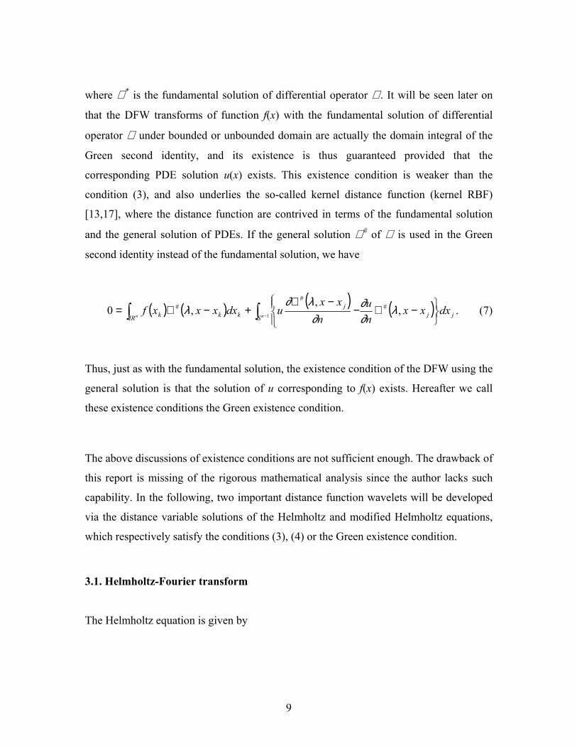
and the general solution of PDEs. If the general solution ℜ # of ℜ is used in the Green

second identity instead of the fundamental solution, we have

( ) ( ) ( ) ( ) jjS

j

IR kkk dxxxnu

nxx

udxxxxfnn

−ℜ

−−ℜ

+−ℜ= ∫∫ −,

,,0 #

##

1λ

∂∂

∂λ∂

λ . (7)

Thus, just as with the fundamental solution, the existence condition of the DFW using the

general solution is that the solution of u corresponding to f(x) exists. Hereafter we call

these existence conditions the Green existence condition.

The above discussions of existence conditions are not sufficient enough. The drawback of

this report is missing of the rigorous mathematical analysis since the author lacks such

capability. In the following, two important distance function wavelets will be developed

via the distance variable solutions of the Helmholtz and modified Helmholtz equations,

which respectively satisfy the conditions (3), (4) or the Green existence condition.

3.1. Helmholtz-Fourier transform

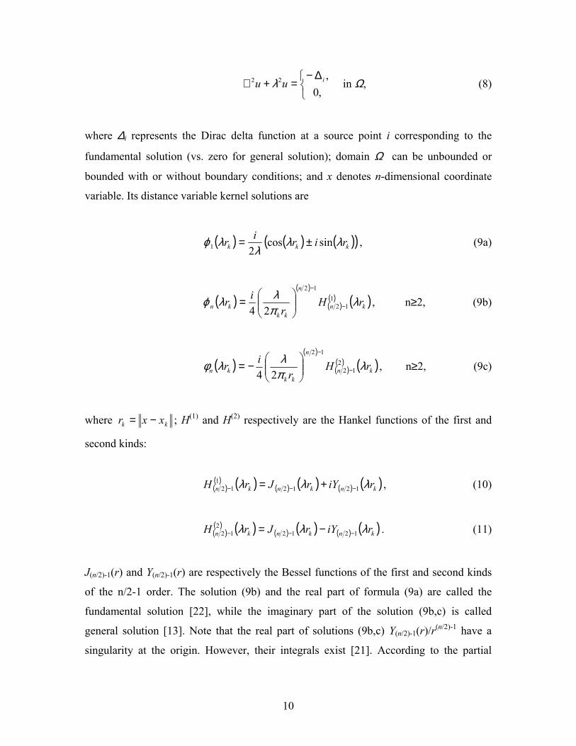
The Helmholtz equation is given by

9

∆−

=+∇,0

,22 iuu λ in Ω, (8)

where ∆i represents the Dirac delta function at a source point i corresponding to the

fundamental solution (vs. zero for general solution); domain Ω can be unbounded or

bounded with or without boundary conditions; and x denotes n-dimensional coordinate

variable. Its distance variable kernel solutions are

( ) ( ) ( )( kkk ririr λλλ

λϕ sincos21 ±= ) , (9a)

( )( )

( )( ) ( kn

n

kkkn rH

rir λ

πλλϕ 1

12

12

24 −

−

= ), n≥2, (9b)

( )( )

( )( ) ( )kn

n

kkkn rH

rir λ

πλλφ 2

12

12

24 −

−

−= , n≥2, (9c)

where kk xxr −= ; H(1) and H(2) respectively are the Hankel functions of the first and

second kinds:

( )( ) ( ) ( ) ( ) ( ) ( knknkn riYrJrH λλλ 12121

12 −−− += ) , (10)

( )( ) ( ) ( ) ( ) ( ) ( knknkn riYrJrH λλλ 12122

12 −−− −= ) . (11)

J(n/2)-1(r) and Y(n/2)-1(r) are respectively the Bessel functions of the first and second kinds

of the n/2-1 order. The solution (9b) and the real part of formula (9a) are called the

fundamental solution [22], while the imaginary part of the solution (9b,c) is called

general solution [13]. Note that the real part of solutions (9b,c) Y(n/2)-1(r)/r(n/2)-1 have a

singularity at the origin. However, their integrals exist [21]. According to the partial

10

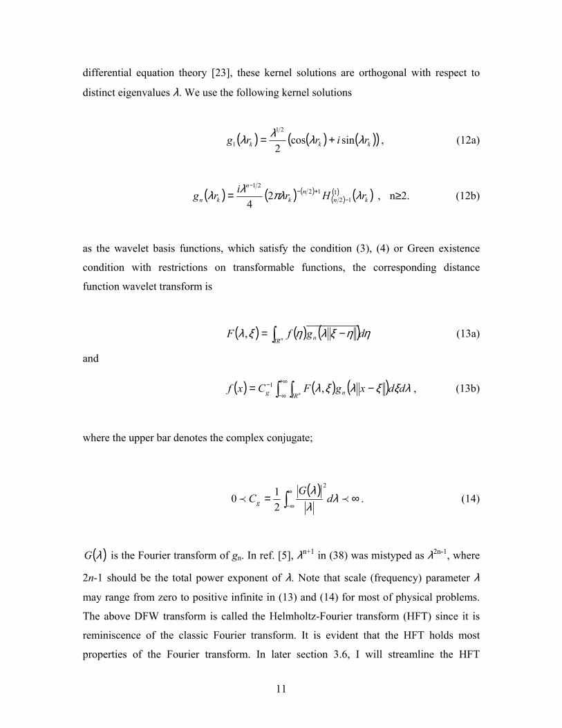
differential equation theory [23], these kernel solutions are orthogonal with respect to

distinct eigenvalues λ. We use the following kernel solutions

( ) ( ) ( )( kkk rirrg λλλλ sincos2

21

1 += ) , (12a)

( ) ( ) ( )( )( ) ( )kn

nk

n

kn rHrirg λπλλλ 112

1221

24 −

+−−

= , n≥2. (12b)

as the wavelet basis functions, which satisfy the condition (3), (4) or Green existence

condition with restrictions on transformable functions, the corresponding distance

function wavelet transform is

( ) ( ) ( ) ηηξληξλ ∫ −=nIR n dgfF , (13a)

and

( ) ( ) ( )∫ ∫+∞

∞−

− −=nIR ng ddxgFCxf λξξλξλ ,1 , (13b)

where the upper bar denotes the complex conjugate;

( )∞= ∫

∞

∞−pp λ

λλ

dG

Cg

2

210 . (14)

( )λG is the Fourier transform of gn. In ref. [5], λn+1 in (38) was mistyped as λ2n-1, where

2n-1 should be the total power exponent of λ. Note that scale (frequency) parameter λ

may range from zero to positive infinite in (13) and (14) for most of physical problems.

The above DFW transform is called the Helmholtz-Fourier transform (HFT) since it is

reminiscence of the classic Fourier transform. It is evident that the HFT holds most

properties of the Fourier transform. In later section 3.6, I will streamline the HFT

11

expression by using a new symbol system. The appendix lists simpler expressions of

some basis function gn in terms of sine and cosine functions.

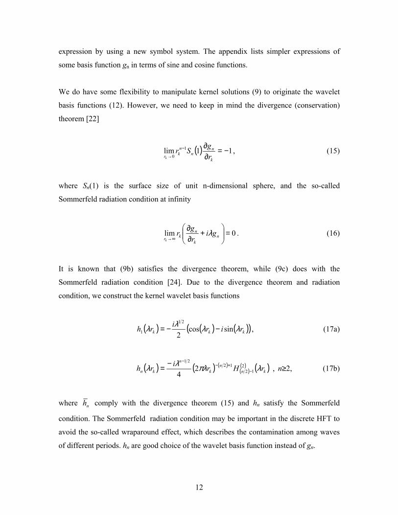
We do have some flexibility to manipulate kernel solutions (9) to originate the wavelet

basis functions (12). However, we need to keep in mind the divergence (conservation)

theorem [22]

( ) 11lim 1

0−=

∂∂−

→k

nn

nkr r

gSrk

, (15)

where Sn(1) is the surface size of unit n-dimensional sphere, and the so-called

Sommerfeld radiation condition at infinity

0lim =

+

∂∂

∞→ nk

nkr

girgr

k

λ . (16)

It is known that (9b) satisfies the divergence theorem, while (9c) does with the

Sommerfeld radiation condition [24]. Due to the divergence theorem and radiation

condition, we construct the kernel wavelet basis functions

( ) ( ) ( )( kkk ririrh λλλλ sincos2

21

1 −−= ), (17a)

( ) ( ) ( )( )( ) ( kn

nk

n

kn rHrirh λπλλλ 212

1221

24 −

+−−−= ) , n≥2, (17b)

where nh comply with the divergence theorem (15) and hn satisfy the Sommerfeld

condition. The Sommerfeld radiation condition may be important in the discrete HFT to

avoid the so-called wraparound effect, which describes the contamination among waves

of different periods. hn are good choice of the wavelet basis function instead of gn.

12

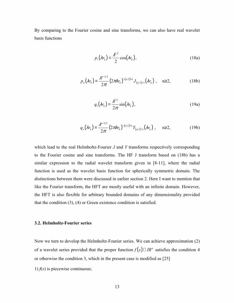
By comparing to the Fourier cosine and sine transforms, we can also have real wavelet

basis functions

( ) ( kk rrp λλλ cos2

21

1 = ), (18a)

( ) ( ) ( )( ) ( )kn

nk

n

kn rJrrp λπλπ

λλ 1212

21

22 −

+−−

= , n≥2, (18b)

( ) ( kk rrq λπ

λλ sin2

21

1 = ) , (19a)

( ) ( ) ( )( ) ( )kn

nk

n

kn rYrrq λπλπ

λλ 1212

21

22 −

+−−

= , n≥2, (19b)

which lead to the real Helmholtz-Fourier J and Y transforms respectively corresponding

to the Fourier cosine and sine transforms. The HF J transform based on (18b) has a

similar expression to the radial wavelet transform given in [8-11], where the radial

function is used as the wavelet basis function for spherically symmetric domain. The

distinctions between them were discussed in earlier section 2. Here I want to mention that

like the Fourier transform, the HFT are mostly useful with an infinite domain. However,

the HFT is also flexible for arbitrary bounded domains of any dimensionality provided

that the condition (3), (4) or Green existence condition is satisfied.

3.2. Helmholtz-Fourier series

Now we turn to develop the Helmholtz-Fourier series. We can achieve approximation (2)

of a wavelet series provided that the proper function satisfies the condition 4

or otherwise the condition 3, which in the present case is modified as [25]

( ) nIRxf ∈

1) f(x) is piecewise continuous;

13

2) ( ) ∞≠−∫−

p01nIR k

nk dxxxxf ;

3) f(x) has bounded variation (or satisfies the Lipschitz condition).

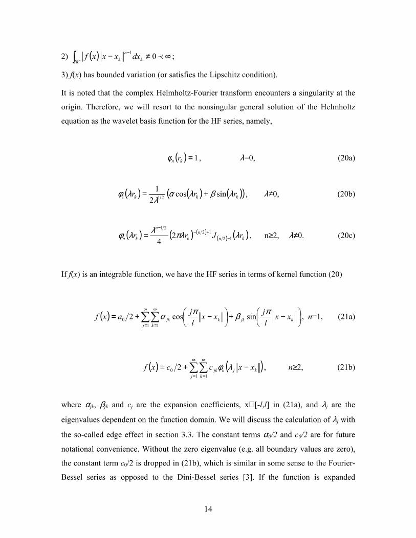
It is noted that the complex Helmholtz-Fourier transform encounters a singularity at the

origin. Therefore, we will resort to the nonsingular general solution of the Helmholtz

equation as the wavelet basis function for the HF series, namely,

( ) 1=kn rφ , λ=0, (20a)

( ) ( ) ( )( kkk rrr λβλαλ

λφ sincos2

1211 += ) , λ≠0, (20b)

( ) ( ) ( )( ) ( kn

nk

n

kn rJrr λπλλλφ 1212

21

24 −

+−−

= ) , n≥2, λ≠0. (20c)

If f(x) is an integrable function, we have the HF series in terms of kernel function (20)

( ) ∑∑∞

=

∞

=

−+

−+=

1 10 sincos2

j kkjkkjk xx

ljxx

ljaxf πβπα , n=1, (21a)

( ) ( kjnj k

jk xxccxf −+= ∑∑∞

=

∞

=

λφ1 1

0 2 ) , n≥2, (21b)

where αjk, βjk and cj are the expansion coefficients, x∈ [-l,l] in (21a), and λj are the

eigenvalues dependent on the function domain. We will discuss the calculation of λj with

the so-called edge effect in section 3.3. The constant terms α0/2 and c0/2 are for future

notational convenience. Without the zero eigenvalue (e.g. all boundary values are zero),

the constant term c0/2 is dropped in (21b), which is similar in some sense to the Fourier-

Bessel series as opposed to the Dini-Bessel series [3]. If the function is expanded

14

spherically symmetrically within a local unit circle, λj in (21b) are the zeros of φn (n≥2)

as nonuniform scale parameters. The convergence of the Helmholtz-Fourier series (21) is

guaranteed uniform and compact due to the condition (3). Need to mention that the

formulas in [6,7] have some errors since I introduced the erroneous weighting function

in the distance function expansion series as well as in the continuous DFW’s. 1−nkr

It is stressed that unlike the RFW [8-11], the DFW expansions are not necessary to be

carried out under a spherically symmetric domain. The strength of the distance function

wavelet series lies in that it is very flexible to any scattered data under arbitrary domain

geometry. The truncating of scale and translation parameters enables the series (21) very

flexible to analysis and practical computations. Furthermore, the thresholding as in the

standard wavelets will produce the sparse matrix and dramatically enhance computing

efficiency. Compared with the so-called fast RBF, which uses the fast multipole method,

domain decomposition or wavelets preconditioning to yield a sparse distance function

matrix, the DFW is a pure fast distance function technique.

By analogy with the convergence and completeness theory of the Fourier series on finite

intervals [23], we could respectively have pointwise, uniform, and mean-square (or L2)

convergences dependent on different conditions of function f(x) on finite domains, which

are weaker than the condition 3 for an unbounded domain. I guess that the conditions for

these three notions of convergence are the same as those required for the Fourier series.

In L2 theory, the corresponding Parseval’s equality is also established, i.e.

( ) ∑∑∫ = 22jkIR

cdxxfn

. (22)

[5] demonstrates all the eigenvalues of the Helmholtz equation with eigenfunctions (20)

are real. According to theorem I in [Chap. 10, 23], the eigenfunctions that correspond to

distinct eigenvalues are necessarily orthogonal. All eigenfunctions corresponding to the

15

same eigenvalue may be chosen to be orthogonal. Therefore, the evaluation of the

expansion coefficients could be easily accomplished via the orthogonality relationships.

In addition, due to theorem II in [Chap. 11, 23], the eigenfunctions are complete in the L2

sense for both the Dirichlet and Neumann problems.

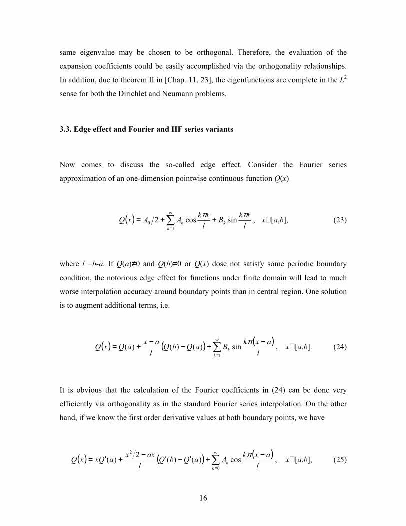
3.3. Edge effect and Fourier and HF series variants

Now comes to discuss the so-called edge effect. Consider the Fourier series

approximation of an one-dimension pointwise continuous function Q(x)

( ) ∑∞

=

++=1

0 sincos2k

kk lxkB

lxkAAxQ ππ , x∈ [a,b], (23)

where l =b-a. If Q(a)≠0 and Q(b)≠0 or Q(x) dose not satisfy some periodic boundary

condition, the notorious edge effect for functions under finite domain will lead to much

worse interpolation accuracy around boundary points than in central region. One solution

is to augment additional terms, i.e.

( ) ( ) ( )∑∞

=

−+−−+=1

sin)()()(k

k laxkBaQbQ

laxaQxQ π , x∈ [a,b]. (24)

It is obvious that the calculation of the Fourier coefficients in (24) can be done very

efficiently via orthogonality as in the standard Fourier series interpolation. On the other

hand, if we know the first order derivative values at both boundary points, we have

( ) ( ) ( )∑∞

=

−+′−′−+′=0

2

cos)()(2)(k

k laxkAaQbQ

laxxaQxxQ π , x∈ [a,b], (25)

16

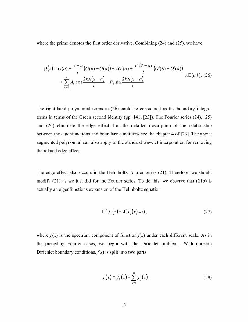
where the prime denotes the first order derivative. Combining (24) and (25), we have

( ) ( ) ( )( ) ( )

laxkB

laxkA

aQbQl

axxaQxaQbQl

axaQxQ

kk

k−+−+

′−′−+′+−−+=

∑∞

=

ππ 2sin2cos

)()(2)()()()(

0

2

x∈ [a,b]. (26)

The right-hand polynomial terms in (26) could be considered as the boundary integral

terms in terms of the Green second identity (pp. 141, [23]). The Fourier series (24), (25)

and (26) eliminate the edge effect. For the detailed description of the relationship

between the eigenfunctions and boundary conditions see the chapter 4 of [23]. The above

augmented polynomial can also apply to the standard wavelet interpolation for removing

the related edge effect.

The edge effect also occurs in the Helmholtz Fourier series (21). Therefore, we should

modify (21) as we just did for the Fourier series. To do this, we observe that (21b) is

actually an eigenfunctions expansion of the Helmholtz equation

( ) ( ) 022 =+∇ xfxf jjj λ , (27)

where fj(x) is the spectrum component of function f(x) under each different scale. As in

the preceding Fourier cases, we begin with the Dirichlet problems. With nonzero

Dirichlet boundary conditions, f(x) is split into two parts

( ) ( ) ( )∑∞

=

+=1

0j

j xfxfxf , (28)

17

where f0(x) and the sum term respectively represent the solutions corresponding to

nonzero boundary condition and zero boundary condition. Since f0(x) is related to zero

eigenvalue, the corresponding Helmholtz equation degenerates into a Laplace equation

( ) 002 =∇ xf (29)

with the nonzero Dirichlet boundary condition. In terms of the Green second identity, we

have

( ) ( ) ( ) ( ) ( )j

jLjS jL

j dxn

xxuxfxxu

nxf

xfn

−

−−= ∫ − ∂∂

∂∂ *

*0 1

, (30)

where uL* is the Laplacian fundamental solution and Sn-1 are the surface of finite

domains. The Neumann boundary data in (30) can be easily evaluated by the boundary

element method (BEM), and then f0(x) at any location can be calculated via (30). The

boundary knot method [5] is also an alternative to the BEM for this task. The HF series

(21b) is modified as

( ) ( ) ( kjnj k

jk xxxfxf −+= ∑∑∞

=

∞

=βλφβ

1 10 ), n≥2, (31)

where the nonzero eigenvalue λβj are calculated with zero Dirichlet boundary condition.

( ) 0det =− kin xxβλφ , n≥2. (32)

18

For a detailed description of a more efficient BKM scheme calculating λβj see [5]. For

brevity, we do not touch on the 1D HF series (21a) too. The expansion coefficients in

(31) can be efficiently calculated via the orthogonality of eigenfunctions

( ) ( )[ ] ( )( )∫

∫Ω

Ω

−

−−=

dxxx

dxxxxfxf

kjn

kjnpjk 2

β

β

λφ

λφβ . (33)

(33) also resembles another way handling inhomogeneous boundary data, which uses the

expansion expression of nonzero boundary values and evaluates the inhomogeneous

effect at each scale separately (pp. 141, [23]).

On the other hand, considering the inhomogeneous Neumann boundary conditions, we

have expansion series

( ) ( ) ( kjnj k

jk xxxfxf −+= ∑∑∞

=

∞

=αλφα

1 10 ), n≥2. (34)

Here the difference is that the Neumann boundary data are known and the Dirichlet

boundary data in (30) need to be evaluated here via the BEM or BKM. Another

distinction is in the evaluation of eigenvalues, namely, we have

( )0det =

∂−∂

i

kin

nxxαλφ

, n≥2. (35)

The corresponding expansion coefficient can be evaluated via the orthogonality as (33).

19

Consider both the inhomogeneous Dirichlet and Neumann boundary data simultaneously

we have expansion series

( ) ( ) ( ) (∑∑∞

=

∞

=

−+−+=1 1

0j k

kjnjkkjnjk xxxxxfxf βα λφβλφα ) , n≥2, (36)

As an alternative way, we can create a different basis function for the inhomogeneous

Dirichlet boundary data from that for the inhomogeneous Neumann data. qn in (19b) is an

ideal choice, but since qn is singular at the origin we could not use it. Instead, the

following expansion is suggested:

( ) ( ) ( kjnj k

jk xxxfxf −′+= ∑∑∞

=

∞

=βλφβ

1 10 ), n≥2, (37)

where the prime denotes the first order derivative of φn with respect to rk. Note that nφ′ is

employed as the basis function instead of φn in (31) since the former has the zero root

while the latter has not. nφ′ is infinitely differential as φn. Similar to (32), the nonzero

eigenvalues λβj are calculated with zero Dirichlet boundary condition.

( ) 0det =−′ kin xxβλφ , n≥2. (38)

The expansion coefficients in (37) can be efficiently calculated via the orthogonality. For

general cases, we can combine (34) and (37) to produce

( ) ( ) ( ) (∑∑∞

=

∞

=

−′+−+=1 1

0j k

kjnjkkjnjk xxxxxfxf λφβλφα ), n≥2. (39)

20

The eigenvalues λ can be calculated by

( ) ( )( ) ( ) 0det =

∂−′∂

∂−∂

−′−

i

kin

i

kin

kinkin

nxx

nxx

xxxxλφλφλφλφ

, n≥2. (40)

nφ′ in (39) serves an analogous role as does the sine function in the standard Fourier

series. In other words, nφ′ acts as a substitute of the singular qn in (19b) to constitute a

complete pair of nonsingular periodic distance basis functions with φn. For instance, the

solutions of the 2D Helmholtz equation are J0, the nonsingular Bessel function of the first

kind of the zero order, and Y0, the singular Bessel function of the second kind of the zero

order. The first order derivative of J0 is minus J1, the nonsingular Bessel function of the

first kind of the first order. It is observed that J1 behaves very much like Y0 except around

the origin, where, unlike the latter, the former has no singularity. In fact, both J1 and Y0

rapidly tend to be indistinguishable away from the origin. The local maximums and

minimums of J0 and J1 periodically appear in a staggered way very closely as do the

cosine and sine functions. In contrast, J1 is a skew-symmetric function as sine function,

while J0 is a symmetric function as cosine function. J1 could act as a suitable replacement

of Y0. Interestingly, it is also found that Y1, the Bessel function of the second kind of the

first order, behaves closely as -J0 off the origin. It is expected that the similar behaviors

exist for the solutions of high dimension Helmholtz equation and their derivatives.

Note f0(x) in all the above expansion is calculated via (30). Comparing (36) and (39) with

(21b), one can note that the former two have the same form of (21a) and (26). Compared

with the standard distance function interpolation (e.g. the thin plate spline), it is very

clear that all the expansion representations given in this section are the multiscale

approximation, while the standard approach is equivalent to the approximation of f0(x).

For the window Fourier transform and the HFT in finite domains, the same strategy can

be used to avoid the edge effect. It is noted that the HF series and transform may be

21

understood the distance variable generalization of the Fourier-Bessel series and Hankle

transform, both of which use the coordinate variable for cylindrically symmetric domain

problems.

3.4. Variants of Helmholtz-Fourier transform

The limiting form of (31) and (34) could be

( ) ( )( ) ( )[ ] ( )

( ) ( )∫ ∫∫

∫∞+

ΩΩ

Ω −−

−−+=

0 2

00 λλφ

λφ

λφddxxx

dxxx

dxxxxfxfxfxf kkn

kn

kn. (41)

Thus, we have the HF J transform in finite domains

( ) ( ) ( )[ ] ( xdxxxfxfC

xF knJ

k ∫Ω −−= λφλ 01, ) (42a)

and

( ) ( ) ( ) ( )∫ ∫+∞

Ω−+=

00 , λλφλ ddxxxxFxfxf kknk , (42b)

where

( )∫Ω −= dxxxC knJ2λφ . (43)

In the cases domain Ω in (42) and (43) is infinite, we have

( ) ( ) ( xdxxxfC

xF knJ

k ∫Ω −= λφλ 1, ) (44a)

22

and

( ) ( ) ( )∫ ∫+∞

Ω−=

0, λλφλ ddxxxxFxf kknk . (44b)

f0(x) is removed here since f(x) tends to zero at infinity.

In order to construct the integral transform corresponding to the HF series (39), we create

the complex basis function

( ) ( ) ( knknkn xxixxxx −−−′=− λϕλϕλ )ψ , (45)

where nψ complies with the divergence theorem (15) and ψn satisfies the Sommerfeld

condition (16). Thus, the infinite domain integral transform can be written as

( ) ( ) ( ) xdxxxfxF knk ∫Ω −= λψλ , (46a)

and

( ) ( ) ( )∫ ∫+∞

Ω−=

0,1 λλψλ

ψ

ddxxxxFC

xf kknk . (46b)

3.5. Helmholtz-Laplace transform

It is noted that as with the Fourier transform, many important functions may not satisfy

the condition (3) or the Green existence condition for the DFW Helmholtz-Fourier

transform. We also know well that the Laplace transform, based on the coordinate

variable solution of the 1D modified Helmholtz equation, is applicable to many more

functions because of the rapid exponential decay of its kernel function. Similarly, by

using the distance function solution of the modified Helmholtz equation, the Helmholtz-

23

Laplace transform (HLT) [5-7] is developed to accommodate many more functions. The

modified Helmholtz equation is given by

∆

=−∇,0,22 iuu µ in Ω, (47)

where domain Ω can be unbounded or bounded with or without boundary conditions. Its

solutions can be written as

( ) krk erw µµµ −=

2

21

1 , (48a)

( ) ( ) ( )( ) ( )kn

nk

n

kn rKrrw µπµπ

µµ 1212

21

22 −

+−−

= , n≥2; (48b)

( ) krk erw µµµ

2ˆ

21

1 = , (49a)

( ) ( ) ( )( ) ( )kn

nk

n

kn rIrrw µπµπ

µµ 1212

21

22

ˆ −+−

−

= , n≥2, (49b)

where I denotes the modified Bessel function of the first kind which grows exponentially

as rk→∞. In contrast, the function K decays exponentially. Note that (48) are the solution

of both external (outcoming radiation field) and interior (incoming radiation field)

problems, while the general solutions (49) are but the solution of interior problems. The

fundamental solutions (48) are thus chosen as the wavelet basis function. In terms of (3),

we have requirements on expressible functions:

1) f(x) is piecewise continuous;

2) ( ) ( ) ∞≠−∫ p0nIR kkn dxxxwxf σ , where σ is a constant.

The corresponding distance function wavelet transform is

24

( ) ( ) ( ηηξµηξµ ∫ −=nIR n dwfL , ) , Re(µ)>σ. (50a)

The scale parameter µ can also be a complex number as in the Laplace transform. I

contemplate that the inverse HLT can be evaluated in the very similar way as for the

inverse Laplace transform [26], i.e.

( ) ( ) ( )∫ ∫∞+

∞−−=

i

i IR nw

ddxwLC

xfn

γ

γµξξµξµ ˆ,1 , γ>σ. (50b)

The related Dirichlet conditions on function f(x) [23,26] may apply to the HLT too. The

Kontorovich-Lebedev transform [26], which uses the coordinate variable solution of the

modified Bessel equation, may be seen as a special case of the present HLT.

It is also possible to construct the finite Helmholtz-Laplace series via the nonsingular

general solution (49) as did the preceding Helmholtz-Fourier series. The series is a

counterpart of the Dirichlet series or the Z-transform of coordinate variable. For brevity,

the details are omitted here.

3.6. A dimension-dependent function for Helmholtz solutions

Going back to (13), one can clearly notice that with the coordinate variable instead of the

distance variable, the 1D Helmholtz-Fourier transform degenerates into the classic

Fourier transform. Thus, it is fair to say that the Fourier transform is a special case of the

general HFT. Similarly, we can find that the Laplace transform belongs to the general

Helmholtz-Laplace transform. Both the Fourier and Laplace transforms have long been

heavily used in a very broad field of science and engineering. Engineers and scientists

alike have got accustomed to their simple exponential function expression. It is observed

25

that the modified Bessel function of the second kind K(x) behaves as e-x with opposite

signs. To streamline and simplify the expression of Helmholtz transforms of different

dimensions, a dimension-dependent function is introduced

( ) ( )( ) ( )

≥

==

−+−

−

−

−

,2,22

,1,2

1212

21

21

nxKx

neE

nn

n

x

xn

λπλπ

λπ

λ λ

λ x≥0. (51a)

( ) ( )( ) ( )

≥

==

−+−

−

,2,22

,1,2ˆ

1212

21

21

nxIx

neE

nn

n

x

xn

λπλπ

λπ

λ λ

λ x≥0. (51b)

Observing (18) and (19), it is found that the imaginary and real parts of the complex

solutions of the Helmholtz equations of high dimensions exhibit considerable wave

behaviour and correspond respectively to cosine and sine functions. It is known [22]

( )( ) ( ) ( ) ( knkn riK

irH λ

πλ −= −− 12

112

2 ) , (52)

In terms of (52), we have

( ) ( )( )

( ) ( )( ) ( ) ( ) ( )( )

≥+

=+=

−−+−

−

,2,24

,1,sincos2

121212

21

21

nxiYxJxi

nxixE

nnn

nxi

n

λλπλλ

λλπ

λλ x≥0. (53)

With this new symbolic expression, the HFT (13) is restated as

26

( ) ( ) ηηξω ηξω∫ −−=nIR

in

n

dEfC

F 1, (54a)

and

( ) ( )∫ ∫+∞

∞−

−=nIR

xin

n

ddEFC

xf ωξξω ξω,1 . (54b)

The HLT (50) is rewritten as

( ) ( ) ηηξ ηξ∫ −−=nIR

sn dEfsL , , Re(s)>σ (55a)

and

( ) ( )∫ ∫∞+

∞−

−=i

i IR

xsn

nn

dsdEsLW

xfγ

γ

ξ ξξ ˆ,1 , γ>σ. (55b)

The Helmholtz-Fourier and Helmholtz-Laplace transforms are now expressed in the

convenient notational conventions as in the standard Fourier and Laplace transforms.

4. Applications

As an illustrative example, the Helmholtz-Fourier series is employed to evaluate the

analytical solutions of the high-dimension homogeneous diffusion problems with

homogeneous boundary conditions:

tuu

∂∂=∇

κ12 , , (56) Ω∈x

27

( )( )

∈=

∈=

,,0,,,0,

T

u

Sxn

txuSxtxu

∂∂ , (57) 0≥t

( ) ( ) ,,0, SxxRxu ∈= (58)

where n is the unit outward normal, . By the approach of the separation of

variable, we have

Γ= SSS u U

( ) ( ) 022 =+∇ xvxv γ , (59)

( ) ( ) 02 =+ tTdt

tdT κγ . (60)

Here γ is the separation constant and actually eigenvalue of the system. In ref. 5, Eq. (16)

has a mistype missing c2, and λ in Eqs. (17) and (24) should be λ.

The problem has only nonnegative eigenvalues [23]. For the Robin (radiation) boundary

condition ( 0=+∂ aunu∂ ), the nonnegative eigenvalues holds provided that a≥0. The

solutions of the present diffusion problem is

( ) ( )∑∞

=

−+=1

0

2

21,

jj

tj xveAAtxu jκγ , (61)

where vj(x) are the corresponding eigenfunctions. Since the eigenfunctions must be finite

at the origin, scraping the singular part of the solution of the Helmholtz equation does not

raise the completeness issue. Therefore, the eigenfunctions are (20). In terms of boundary

conditions (57), the eigenvalues of (59) can be efficiently solved by the boundary knot

method [17]. For details see ref. [5]. Thus, the solution can be expressed as

28

( ) (∑∑∞

=

∞

=

− −+=1 1

0

2

21,

j kkjn

tjk xxeAAtxu j γφκγ ), (62)

where φn are given in (20). The Helmholtz-Fourier series solution (62) is valid for any

dimensions and geometry since the approach is independent of dimensionality and

geometry. The coefficient Ajk can be determined by the initial condition (58) with the help

of the orthogonality of the eigenfunctions [5,27], i.e.

( ) ( )( )∫

∫Ω

Ω

−

−=

dxxx

dxxxxRA

kjn

kjnjk 2γφ

γφ. (63)

As far as the author knows, the report is the first attempt to get an analytical solution of

diffusion problems with irregular domain of any dimensions. For a detailed solution of a

wave equation of arbitrary dimensions and geometry see ref. 5. This solution can easily

be extended to diffusion problems with non-homogeneous solution. It is, however,

stressed that the present solution cannot be used for problems with time-dependent

boundary conditions or for problems in unbounded domains since the separation of

variable does not apply to them.

Since the present series solution is wavelets, the Gibbs phenomenon long perplexing the

Fourier series is eliminated. By adapting the scaling parameter (dilations) and translat

rather than the dyadic multiresolution analysis, we get locally supported refinements both

in scale and location. Due to the use of the inseparable distance function, we also avoid

using the tensor-product approach for high dimensional problems with irregular

geometry. In addition, the present method is essentially meshfree.

5. Anisotropic distance function wavelets and ridgelets

The radial basis function is found very efficient for many problems [28]. Carlson and

Foley [29], however, notice that the isotropic RBFs such as the MQ and TPS do not work

29

well for some so-called track data problems. This kind of problems has the characteristics

of preferred direction. In preceding analysis, the isotropic solutions of the Helmholtz

equations were used as the wavelet basis function. In the case of dealing with directional

data problems, we need to create the anisotropic distance function which is competent to

capture the directional property. The solution of the convection-diffusion equation is one

of such choices to serve as the DFW basis function [5,6]. The equation is given by

∆

=−∇•+∇,0,2 ikuuvuD v , in Ω, (64)

where vv denotes velocity vector, D is the diffusivity coefficient, and k represents the

reaction coefficient. The corresponding solutions of translation invariant are

( )( )

kk r

Dxxv

k exxuρρρ

−−⋅−=− 2

21*1 2

,v

, (65a)

( )( )

( ) ( )( ) ( kn

nk

Dxxvn

kn rKrexxuk

ρπρπ

ρρ 12122

21* 2

2, −

+−−⋅−−

=− )v

, n≥2, (65b)

( )( )

kk r

Dxxv

k exxuρρρ

+−⋅−=− 2

21#1 2

,v

, (66a)

( )( )

( ) ( )( ) ( kn

nk

Dxxvn

kn rIrexxuk

ρπρπ

ρρ 12122

21# 2

2, −

+−−⋅−−

=− )v

, n≥2, |(66b)

where dot denotes the dot product of two vectors;

21

2

2

+

=

Dk

Dvv

ρ . (67)

30

Note that both the Euclidean distance variable and the translation distance variable are

associated with the present distance function solutions. Thus, the basis functions are

anisotropic and not rotational invariant “RBF”. (3) or the Green existence condition is the

restrictive condition on expressible function of the convection-diffusion DFW transform.

The solutions (65) are suitable as the wavelet basis function. We have the corresponding

distance function wavelet transform:

( ) ( ) ( ) xdxuxfFnIR n∫ −= ξρξρ ,, * . (68)

The ridgelets [30] are a variant of the wavelets designed for the processing of line or

surface discontinuous data and track data of high dimensions, which play an important

role in neural network and machine learning. A ridgelet function series can be stated as

( ) ( )∑ −= bxxf N αµψˆ , (69)

where α, µ, and b respectively represent the scale, direction, and translate; ψ is the

ridgelet basis function. The DFW (68) could be also seen as the distance function ridgelet

transform with a constant direction. It is worth pointing out that the convection-diffusion

problems are closely related to phenomena of shock with localized great gradient

variations, which precisely fall into the territory of the ridgelets. For varying directional

vector vv , we rewrite (68) as

( ) ( ) ( ) xdxvuxfvFnIR n∫ −= ξκξκ ,,,, * vv . (70)

Unfortunately, we can not have a ridgelet series by simply discretizing (68) or (70) since

multidimensional u* has a singularity at the origin. On the other hand, (66b) is

nonsingular at the origin and actually infinitely continuous but grow exponentially as

rk→∞. Because a ridgelet series is aimed at handling data or PDEs within bounded

domains, the growth at infinity is no longer an issue as in the integral transform on

31

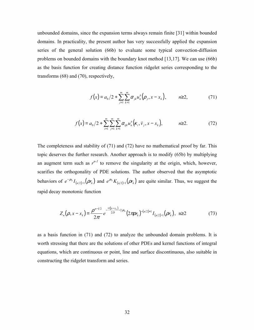
unbounded domains, since the expansion terms always remain finite [31] within bounded

domains. In practicality, the present author has very successfully applied the expansion

series of the general solution (66b) to evaluate some typical convection-diffusion

problems on bounded domains with the boundary knot method [13,17]. We can use (66b)

as the basis function for creating distance function ridgelet series corresponding to the

transforms (68) and (70), respectively,

( ) ( kjnj k

jk xxuaxf −+= ∑∑∞

=

∞

=

,2 #

1 10 ρα ), n≥2, (71)

( ) ( kjini j k

ijk xxvuaxf −+= ∑∑∑∞

=

∞

=

∞

=

,,2 #

1 1 10

vκα ), n≥2. (72)

The completeness and stability of (71) and (72) have no mathematical proof by far. This

topic deserves the further research. Another approach is to modify (65b) by multiplying

an augment term such as rn-1 to remove the singularity at the origin, which, however,

scarifies the orthogonality of PDE solutions. The author observed that the asymptotic

behaviors of ( ) ( knr rIe k ρρ

12 −− ) and ( ) ( kn

r rKe k ρρ12 − ) are quite similar. Thus, we suggest the

rapid decay monotonic function

( )( )

( ) ( )( ) ( kn

nk

rD

xxvn

kn rIrexxZ kk

ρπρπ

ρρρ

12122

221

22

, −+−−−⋅−−

=−v

) , n≥2 (73)

as a basis function in (71) and (72) to analyze the unbounded domain problems. It is

worth stressing that there are the solutions of other PDEs and kernel functions of integral

equations, which are continuous or point, line and surface discontinuous, also suitable in

constructing the ridgelet transform and series.

32

6. Some remarks

The present status of the DFW Helmholtz transforms resembles the immature Fourier’s

work in the early eighteen century. We are moving into an uncharted territory, where a

lot of basic and applied research issues remain yet to be explored. A few things are

uncertain for the DFW’s, among which are the fast algorithm for Helmholtz-Fourier

series and whether the DFW’s basis functions are unconditional [32] and lacking of a

solid mathematical underpinning.

Ref. 5 made a brief comment on the advances of the RBF wavelets, especially for the so-

called pre-wavelets. Very recently, Blu and Unser [33] presented an interesting concept

of central functions to connect the RBF and wavelets. These existing works mostly

follow the philosophy of developing RBF wavelets via a hierarchy multiresolution spline

construction approach, without relating to the solution of PDEs. In contrast, the distance

function wavelets using the kernel distance variable solutions of PDEs are not only

orthogonal but also infinitely differentiable. Some of them are very compactly supported

(e.g. the HLT and the high-dimensional or large scale HFT). Comparing the so-called

local trigonometric bases [34] with the Helmholtz Fourier series and transform, we can

find that the former is a tedious artificial construction of wavelet basis functions without

considering the dimensional effect, while the HF series and transform are a natural simple

PDE-based approach.

The DFW’s also have certain advantages over the standard spline wavelets such as the

popular Daubechies wavelets [21,34]. For instance, the DFW’s have a convenient closed

form expression, while the standard spline wavelets usually have no such formula (it is

defined implicitly through an infinite recursion) [33]. The DFW’s are ideally suited for a

non-uniform setting, while conventional wavelet theory is restricted to uniform grids

[33]. It is noted that the basis functions of DFW’s are non-stationary wavelets and not

dilates of each other. The DFW’s are also rotational (symmetric) or translation invariant,

while the standard spline wavelets are not even translation invariant [34]. As in the

standard wavelets, the proper thresholding will produce very spare matrix of the DFW’s,

33

which eliminates one of the perplexing issue of handling full matrix in the distance

function. Consequently, the DFW is also very promising in data compression and image

processing, especially for edge detection since the DFW’s link the wavelets to the

boundary integral equation method.

Some extended results and conjectures of the DFW are presented in the subsequent

reports II and III [1,2]. As Aslak and Winther [35] put it “The laws of nature are written

in the language of partial differential equations.” this study shows that the wavelets are

certainly not an exception.

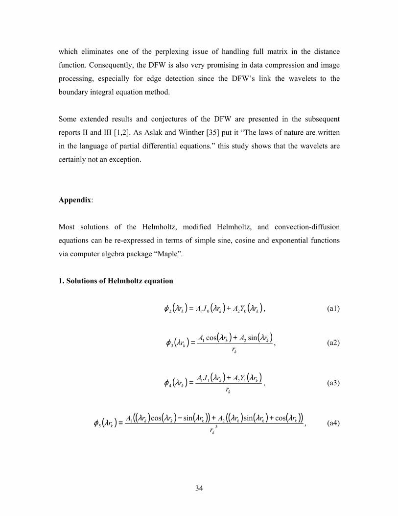
Appendix:

Most solutions of the Helmholtz, modified Helmholtz, and convection-diffusion

equations can be re-expressed in terms of simple sine, cosine and exponential functions

via computer algebra package “Maple”.

1. Solutions of Helmholtz equation

( ) ( ) ( kkk rYArJAr )λλλϕ 02012 += , (a1)

( ) ( ) ( )k

kkk r

rArAr λλλϕ sincos 213

+= , (a2)

( ) ( ) ( )k

kkk r

rYArJAr λλλϕ 12114

+= , (a3)

( ) ( ) ( ) ( )( ) ( ) ( ) ( )( )3

215

cossinsincos

k

kkkkkkk r

rrrArrrAr λλλλλλλϕ ++−= , (a4)

34

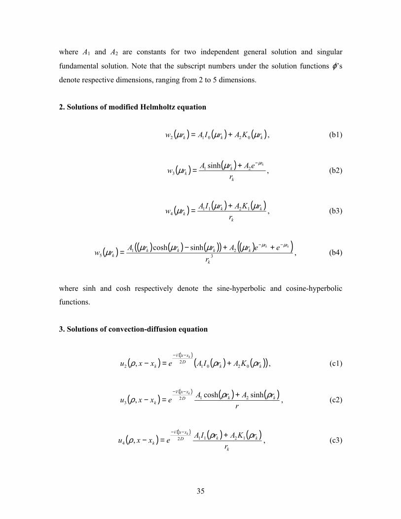
where A1 and A2 are constants for two independent general solution and singular

fundamental solution. Note that the subscript numbers under the solution functions ϕ’s

denote respective dimensions, ranging from 2 to 5 dimensions.

2. Solutions of modified Helmholtz equation

( ) ( ) ( kkk rKArIArw )µµµ 02012 += , (b1)

( ) ( )k

rk

k reArArw

kµµµ−+= 21

3sinh , (b2)

( ) ( ) ( )k

kkk r

rKArIArw µµµ 12114

+= , (b3)

( ) ( ) ( ) ( )( ) ( )( )3

215

sinhcosh

k

rrkkkk

k reerArrrArw

kk µµµµµµµ−− ++−= , (b4)

where sinh and cosh respectively denote the sine-hyperbolic and cosine-hyperbolic

functions.

3. Solutions of convection-diffusion equation

( )( )

( ) ( )( kkD

xxv

k rKArIAexxuk

ρρρ 02012

2 , +=−−⋅−

)v

, (c1)

( )( ) ( ) ( )

rrArAexxu kkD

xxv

k

k ρρρ sinhcosh, 2123

+=−−⋅−v

, (c2)

( )( ) ( ) ( )

k

kkDxxv

k rrKArIAexxu

k ρρρ 121124 , +=−

−⋅− v

, (c3)

35

( )( ) ( ) ( ) ( )( ) ( )( )

3212

5sinhcosh,

k

rrkkkkD

xxv

k reerArrrAexxu

kkk ρρρρρρρ−−−⋅− ++−=−

v

. (c4)

References

1. W. Chen, Distance function wavelets – Part II: Extended results and conjectures,

CoRR preprint, Research report of Simula Research Laboratory, May, 2002.

2. W. Chen, Distance function wavelets - Part III: “Exotic” transform and series, CoRR

preprint, Research report of Simula Research Laboratory, May, 2002.

3. E.A. Gonzalez-Velasco, Fourier Analysis and Boundary Value Problems, Academic

Press, 1995.

4. O. Erosy, Fourier-Related Transforms, Fast Algorithms and Applications, Prentice-

Hall, 1997.

5. W. Chen, Analytical solution of transient scalar wave and diffusion problems of

arbitrary dimensionality and geometry by RBF wavelet series,

http://xxx.lanl.gov/abs/cs.NA/0110055, (CoRR preprint), Research report in

Informatics Department of University of Oslo, 2001.

6. W. Chen, Orthonormal RBF Wavelet and Ridgelet-like Series and Transforms for

High-Dimensional Problem, Int. J. Nonlinear Sci. & Numer. Simulation, 2(2), 155-

160, 2001.

7. W. Chen, Errata and supplements to: Orthonormal RBF Wavelet and Ridgelet-like

Series and Transforms for High-Dimensional Problems, (CoRR preprint),

http://xxx.lanl.gov/abs/cs.NA/0105014, 2001.

8. J. Epperson and M. Frazier, An almost orthogonal radial wavelet expansion for radial

distributions, J. Fourier Anal. Appl., 1(3), 1995.

9. M.A. Mourou and K. Trimeche, Inversion of the Weyl integral transform and the

radon transform on Rn using generalized wavelets, C.R. Math. Rep. Acad. Sci.

Canada, XVIII(2-3), 80-84, 1996.

10. K. Trimeche, Generalized Harmonic Analysis and Wavelet Packets, Gordon &

Breach Sci. Publ., 2001.

36

11. M. Rosler, Radial wavelets and Bessel-Kingman Hypergroups, preprint.

12. P. Hornby, F. Boschetti and F.G. Horowitz, Analysis of Potential Field Data in the

Wavelet Domain, 59th EAGE Conference, Geneva, F35-36, 26-30 May, 1997.

13. W. Chen and M. Tanaka, Relationship between boundary integral equation and radial

basis function, in The 52th Symposium of JSCME on BEM (Tanaka, M. ed.), Tokyo,

2000.

14. M.D. Buhmann, Radial basis functions. Acta Numerica. 1-38. 2000.

15. G.E. Fasshauer and L.L. Schumaker, Scattered Data Fitting on the Sphere. In Math.

Methods for Curves and Surfaces II, pp. 117-166, M. Dæhlen, T. Lyche, and L.L.

Schumaker (eds.), 1998.

16. D. E. Myers, S. De Iaco, D. Posa AND L. De Cesare, Space-Time Radial Basis

Functions, Comput. Math. Appl. 43, 539-549, 2002.

17. W. Chen, New RBF collocation schemes and kernel RBF with applications, in Int.

Workshop for Meshfree Methods for PDEs, Bonn, Germany, 2001 (also see CoRR

preprint, http://xxx.lanl.gov/abs/cs.NA/0111063).

18. H. Wendland and R. Schaback, Characterization and construction of radial basis

functions, in N. Dyn, D. Leviatan, D. Levin and A. Pinkus (eds), Multivariate

Approximation and Applications , Cambridge University Press, Cambridge, 2001.

19. W. Light, Ridge functions, Sigmoidal functions and neural networks, Approximation

Theory VII, (E. W. Cheney, C.K. Chui and L.L. Schumaker eds.), pp. 163-206, 1992.

20. J. Levesley, Y. Xu, W. Light and W. Cheney, Convolution operators for radial basis

approximation, SIAM J. Math. Anal., 27(1), 286-304, 1996.

21. I. Daubechies and W. Sweldens, Factoring Wavelet Transforms into Lifting Steps, J.

Fourier Anal. Appl., 4(3), 247-269, 1998.

22. P.K. Kythe, Fundamental Solutions for Differential Operators and Applications,

Birkhauser, Boston, 1996.

23. W.A. Strauss, Partial Differential Equations, an Introduction, John Wiely & Sons,

1992.

24. N. Kamiya and E. Anoh, A note on multiple reciprocity integral formulation for the

Helmholtz equation, Comm. Numer. Methd. Engng. 9, 9-13, 1993.

37

38

25. M. Abramowitz and I.A. Stegun (ed.), Handbook of Mathematical Functions, Dover

Publ., inc., New York, 1974.

26. B. Davies, Integral Transforms and Their Applications, Springer-Verlag, 1978.

27. I.L. Brunton and A.J. Pullan, A semi-analytic boundary element method for parabolic

problems, Engng. Anal. Boundary Elements, 18, 253-264, 1997.

28. R. Franke, Scattered data interpolation: tests of some methods, Math. Comput. 48

181-200, 1982.

29. R.E. Carlson and T.A. Foley, Interpolation of track data with radial basis methods,

Comput. Math. Appl. 24, 27-34, 1992.

30. E. Candµes and D. Donoho, Ridgelets: the key to high-dimensional intermittency?,

Phil. Trans. R. Soc. Lond. A, 357, 2495-2509, 1999.

31. D.G. Duffy, Transform Methods for Solving Partial Differential Equations, CRC

Press, Florida, 1994.

32. D.L. Donoho, Unconditional bases are optimal bases for data compression and for

statistical estimation. Appl. Comput. Harmonic Anal., 1(1), 100-115, 1993.

33. T. Blu and M.Unser, Wavelets, fractals and radial basis functions, IEEE Trans. Signal

Processing, (to appear), 2002.

34. C.S. Burrus, R.A. Gopinath and H. Guo, Introduction to Wavelets and Wavelet

Transforms, A Primer, Prentice Hall, 1998.

35. A. Tveito and R. Winther, Introduction to Partial Differential Equations; A

Computational Approach, Springers TAM-series vol 29, 1998.