Heterodox Central Banking∗

Luis Felipe Cespedes

Central Bank of Chile

Roberto Chang

Rutgers University

Javier Garcıa-Cicco

Central Bank of Chile

November 2009

1 Introduction

In response to the current global crisis, the U.S. Federal Reserve and other central banks around the

world have implemented a number of diverse policy measures, including purchasing of a wide array

of securities, lending to financial institutions, exchange rate interventions, and paying interest on

reserves. Some central banks have also reduced monetary policy interest rates to minimum levels

(lower bound) and have announced an explicit commitment to keep interest rates at that level for a

prolonged period of time. This array of instruments contrasts with a conventional view, embedded

in dominant models of monetary policy, under which a central bank only controls a short term

interest rate, such as the Federal Funds rate.

Some of the previous actions may be classified as responses to increasing demand for liquidity

in the context of high financial uncertainty. An example of this liquidity provision by central

banks is repo operations to provide US dollar liquidity in many economies in the period around the

bankruptcy of Lehman Brothers. Other actions may be classified as actions implemented to deal

with malfunctioning of financial markets (insufficient lending to non financial firms or high lending

spreads), and actions implemented to deal with the need to enhance the monetary policy stimulus

under the lower bound constraint.

∗We thank Felipe Labbe and Yan Carrire-Swallow for excellent research assistance.

1

This paper discusses theoretical and practical aspects of heterodox policies. In terms of theory,

the paper focuses on the two alternative arguments that have been offered to rationalize such

policies: the desirability of further monetary stimulus when interest rates are already at zero, and

the need to unlock financially intermediated credit when it freezes in a crisis. On the first argument,

we provide a framework to analyze the theoretical mechanisms through which quantitative easing

may be effective to deal with the lower bound constraint. We then show that the effectiveness

of such unconventional policies depends crucially on the ability of the central bank to commit

to future policy, in line with Krugman (1998). Regarding the second argument, we present a

model that helps us to introduce a role for unconventional monetary policy in the context of non

trivial financial intermediation. We then argue that the introduction of financial intermediaries in

a standard models lead to results that challenge conventional wisdom regarding the effects of non

conventional policies.

In terms of recent practice, we provide evidence regarding recent experience of central banks

that have implemented inflation targets in the conduct of monetary policy. We associate the

different monetary policy actions with different phases of the recent financial crisis and with different

objectives. We concentrate our analysis in evaluating actions aimed at increasing the monetary

policy stimulus and dealing with disrupted financial markets.

The rest of the paper is organized as follows. Section 2 presents a theoretical discussion of

two relevant issues that have been at center stage in both policy and academic discussions about

unconventional policies during the current crisis: the role of credibility and the importance of

financial frictions and bank capital. Section 3, on the other hand, provides a more empirically

oriented account of recent events. We first discuss the timing and the type of unconventional

policies that have been implemented. We then compare several alternative measures that can be

used to assess the stance of monetary policy, particularly when the policy rate has reached its lower

bound. Finally, we provide descriptive evidence on the effects of these policies on the shape of the

yield curve and the lending-deposit spreads. Section 4 concludes.

2

2 Rationalizing Hetedorox Monetary Policy

2.1 Monetary Policy at the Edge: The Role of Credibility

One often mentioned justification for unconventional monetary policy is that the usual monetary

instrument, the control of an overnight interest rate in the interbank market, may have reached a

limit. In particular, this is the case when a monetary stimulus is deemed to be desirable but the

policy rate is a nominal one that cannot be pushed below zero (or a value slightly greater than

zero). If the policy rate is already at or close to the lower bound, the central bank is forced to look

for alternative ways to provide the monetary stimulus.

Clearly, the current crisis has brought several countries to a situation in which policy interest

rates are close to zero but expansionary policy appears warranted. Much less clear, however, is

whether that fact is sufficient to justify the kind of unconventional policies that we have observed

in practice. Can one appeal to the zero lower bound problem to rationalize, for example, the

striking expansion in the size of the Federal Reserve’s balance sheet as well as the changes in its

composition? Here we argue that the answer can be positive or negative, depending on the policy

environment and, especially, on the central bank’s ability to commit to future policy.

The starting point of our argument is the observation that currently accepted macroeconomic

theory implies that the zero bound on interest rates will rarely, if ever, be a truly binding constraint

for a central bank that can perfectly commit in advance to future policy. Current theories emphasize

that a central bank can affect current economic decisions not only through the current setting of its

policy instrument (e.g. today’s interest rate) but also, and perhaps much more effectively, through

its impact on the public’s expectations of the future settings of the instrument. The corollary is

that the central bank can always provide some stimulus to the economy, even if the policy rate is

at the zero bound, by committing to reducing future policy rates below levels previously expected

(which is itself feasible if the policy rate was expected to be positive at some point in the future).

Thus, for example, Bernanke and Reinhart (2004, page 85) argue that one of the available

strategies for ”stimulating the economy that do not involve changing the current value of the policy

rate...[is] providing assurance to financial investors that short rates will be lower in the future

3

than they currently expect”. The same argument has been embraced recently by the European

Central Bank (Bini Smaghi 2009), the Bank of Canada (Murray 2009), and others. In fact, even

Krugman’s (1998) pioneering discussion of Japan implied that the Bank of Japan could have escaped

the liquidity trap there by promising to keep interest rates sufficiently low for some period even

after inflation had become positive (see also Svensson 2003).

In short, the zero lower bound on interest rates is unlikely to be a serious constraint on a central

bank that can precommit policy. One could conjecture, however, that unconventional policies such

as ”quantitative easing” or ”credit easing” may be still be useful to complement conventional policy.

Somewhat surprising, however, is to realize that that conjecture is quite unlikely to hold.

This key point has been developed most convincingly by Eggertsson and Woodford (2003).

They show that, once a strategy for setting current and future policy rates is in place (for example,

by a rule of the Taylor type), real allocations and asset prices are independent of what the central

bank does with the composition or size of its balance sheet in periods in which the policy rate is

zero.

It may be worth expanding on the intuition behind this important result, if only to stress its

generality. Eggertsson and Woodford’s model is a variant of the canonical New Keynesian sticky

price model developed by Woodford (2003) and others. In that model, as well as many others,

all asset prices are determined once the equilibrium pricing kernel or stochastic discount factor is

given. Likewise, the stochastic discount factor determines the relevant budget constraint of the

household, and the pricing decisions of producers.

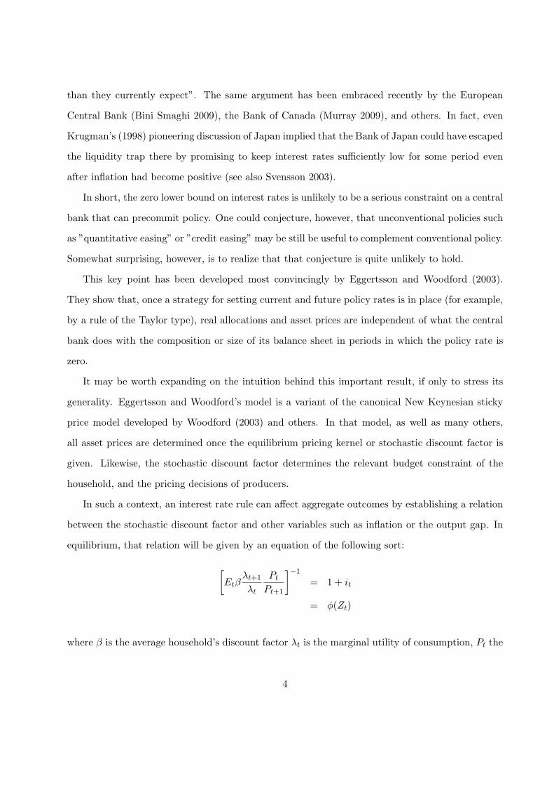
In such a context, an interest rate rule can affect aggregate outcomes by establishing a relation

between the stochastic discount factor and other variables such as inflation or the output gap. In

equilibrium, that relation will be given by an equation of the following sort:

[

Etβλt+1

λt

Pt

Pt+1

]

−1

= 1 + it

= φ(Zt)

where β is the average household’s discount factor λt is the marginal utility of consumption, Pt the

4

price of consumption, it the nominal interest rate for loans between periods t and t + 1, and φ is

a function of a vector of variables Zt, typically inflation and output. The first equality reflects the

household’s optimal portfolio decisions; here, the stochastic discount factor is given by the random

variable βλt+1/λt. The second equality says that the central bank sets the interest rate it as a

function φ of the vector of variables Zt. So, in equilibrium, interest rate policy (e.g. a choice of

the function φ as well as the vector Zt) implies a relation between the stochastic discount factor,

inflation, and the vector Zt. Indeed, this is the main (and often the only) way in which interest

rate policy affects aggregate outcomes.

If the zero bound on the policy rate it were not a binding constraint, a choice of an interest

rate rule φ(Zt) would leave no room for ”quantitative easing”, that is, independent control of the

monetary base. The quantity of money would be determined by its demand, with the central bank

adjusting the base as necessary to clear the market (this is indeed what an interest rate rule would

mean). In addition, under usual assumptions on fiscal policy, changes in the composition of the

central bank’s balance sheet (and, more generally, of the consolidated government) are irrelevant

for aggregate outcomes. This is because the latter can be shown to depend only on the present

value budget constraint of the government, which is given by its initial debt plus the appropriately

discounted value of (possibly state contingent) fiscal deficits.

Eggertsson and Woodford (2003) extend this logic to situations in which the interest rate policy

φ(Zt) may prescribe a zero interest rate under some circumstances (i.e. for some values of the

vector Zt). In those cases, they assume that the demand for money is indeterminate (the real

demand for money being only bounded below by some satiation level). This allows the central

bank to determine the quantity of money independently, in other words, to engage in ”quantitative

easing”. They show, however, that aggregate allocations are independent of the details of such

quantitative easing. The logic is simple: as we just discussed, quantitative easing might affect

aggregate outcomes if it had some impact on the stochastic discount factor. But the latter is

pinned down by the function φ, as in the absence of the lower bound problem.

The justification for the last assertion is illuminating. The assertion would be immediate if

the marginal utility of consumption, λt, were independent of real money balances. Eggertsson and

5

Woodford assume, however, that utility may depend on real balances in a nonseparable way, so λt

may depend on Mt/Pt. However, if the interest rate is driven to zero, real balances must exceed

the satiation level, which in turn means that the quantity of money has no longer any effect on

utility and, a fortiriori, on λt. (It is in this exact sense that money and bonds becoming perfect

substitutes at zero interest rates matters.)

Having established that quantitative easing is irrelevant at zero interest rates, the irrelevance

of altering the composition of the central bank’s balance sheet follows in the same way as before.

Our discussion (hopefully) stresses that the logic behind the Eggertsson-Woodford irrelevance

result is quite general and, hence, extends to a very wide class of models, including most currently

in fashion. The result, in particular, does not hinge on the absence of imperfectly substitutable

assets, which may have led some to suspect that changes in the size and composition of the central

bank balance sheets would have ”portfolio balance” effects. Indeed, the absence of portfolio balance

effects could be taken to be a significant flaw, and one could conjecture that models featuring such

effects may overturn the irrelevance argument. But a compelling portfolio balance model of the

effects of policies regarding the balance sheet of the central bank is yet to be developed. In addition,

the empirical evidence about portfolio balance effects provides little support for them, as stressed

by Bernanke and Reinhart (2004): ”the limited empirical evidence suggests that, withing broad

classes, assets are close substitutes, so that changes in relative supplies of the scale observed in U.S.

experience are unlikely to have a major impact on risk premiums or even term premiums (Reinhart

and Brian Sack, 2000)”.

Summarizing, we have argued that a central bank that can commit in advance to a conventional

interest rate policy will generally not find that the zero bound on interest rates is a binding restric-

tion and, in particular, can provide a monetary stimulus even in a liquidity trap by promising that

future settings of the policy rate will be lower than they would have been otherwise. In addition,

such a central bank will find that quantitative easing, portfolio management maneuvers, and other

strategies for altering the size and composition of its balance sheet at times of zero interest rates

are irrelevant.

This given, why is then the case that, often, central banks have been unable to come out of

6

deflationary liquidity traps by just promising expansionary policy in the future? The key conjecture

is that such promises may not be credible. Credibility as a crucial constraint in this situation has,

of course, been emphasized by several authors, starting with Krugman in his (1998) analysis of the

Japanese recession.

One implication of this observation is that the literature is full of warnings and admonitions

about the need for central banks to ensure that announcements of future policy are believable,

suggesting even that central banks can ”manage expectations” independently of interest rate policy.

For example, the Banque of France recently stated that one unconventional policy is ”influencing

the yield curve by guiding expectations” (Banque of France 2009, page 5). There is little guidance

in these statements, however, as to how precisely the central bank can independently manage

expectations. Bernanke and Reinhart (2004, p.86) acknowledged this fact, stating: ”Ultimately,

however, the central bank’s best strategy for building credibility is to build trust by ensuring that

its deeds match its words...the shaping of expectations is not an independent policy instrument in

the long run. ”

Others have responded to the credibility issue by emphasizing the need for improving ”trans-

parency” and ”clear communication ” of central bank policy intentions. Of course, it is hard to

argue with the view that transparency and clear communication are desirable aspects of central

bank policy. But, aside from the fact that it is not clear why the need for them is greater when

interest rates are close to zero than at other times, there is no generally accepted theory of how

more or less transparency affects monetary transmission channels.

A related claim, of particular relevance to our discussion, is that changes in the size and compo-

sition of the central bank balance sheet can help the credibility of the central bank’s announcements

about future policy. And, in fact, some authors have claimed that this is the main role of uncon-

ventional policies. For example, Bernanke and Reinhart (2004, p. 88) argue that a central bank

policy of setting a high target for bank reserves ”...is more visible, and hence may be more credible,

than a purely verbal promise about future short term interest rates. ” Likewise, Eggertsson and

Woodford (2003) conjectured that ”shifts in the portfolio of the central bank could be of some value

in making credible to the private sector the central bank’s own commitment to a particular kind of

7

future policy... ’Signalling ’ effects of this kind...might well provide a justification for open market

policy when the zero bound binds. ”

To date, however, attempts to make these claims more precise are lacking. But a long standing

theory of monetary policy under imperfect credibility suggests several ways to develop this view.

To illustrate, let us examine the implications of a simple model of monetary policy.

2.1.1 Unconventional Policy: An Illustrative Model

We shall extend the model of Jeanne and Svensson (2007, henceforth JS). Consider a small open

economy with a representative agent that maximizes the discounted expected utility of money

holdings and consumption of tradables and nontradables. The period utility of tradables is log Ct,

where Ct is a Cobb Douglass aggregate of home (h) nontradeables and foreign (f) tradables

Ct = C1−αht Cα

ft

Cht is, in turn, a conventional Dixit Stiglitz aggregate of domestic varieties. With the world

price of foreign tradables normalized at one, the price of consumption is, therefore

Pt = P 1−αht Sα

t

where Pht is the price of home nontradables and St the nominal exchange rate.

The representive agent chooses consumption and the holdings of money, a world noncontingent

bond, and domestic bonds. His sources of income in each period are wages, profits of domestic

firms, income from previous investments, and a transfer from the central bank (Z in JS). It turns

out that these transfers are not needed for our argument, but let us keep them in for now to preserve

the notation of JS.

There is a central bank that can print domestic currency freely to finance transfers and a

portfolio of securities. A bond of maturity k is a promise to pay one unit of consumption at time

t + k. For simplicity, assume that k can be either one or two, e.g. there are ”short” (one period)

8

bonds and ”long” (two period) bonds. 1

Let Qst denote the home currency price at t of a bond promising one unit of consumption at

t + s, s = 1, 2. Letting Bst be the central bank holdings at the end of period t of the corresponding

bond, the central bank’s budget constraint is

Zt + Q1t B

1t + Q2

t B2t = Mt − Mt−1 + B1

t−1 + Q1t B

2t−1

In contrast with JS, who examine the role of foreign exchange intervention, we assume that

the central bank keeps zero foreign exchange reserves. Instead, it holds a portfolio of short and

long bonds. This means that, in the central bank’s budget constraint, the crucial term will be the

last one in the RHS, which denotes the current value of long bonds purchased the previous period.

Hence, changes in the price of long bonds can be a source of gains or losses for the central bank.

JS prove two results. The first one is that a central bank that minimizes a conventional

expected discounted value of losses that depend only on inflation and the output gap may be

unable to implement an optimal policy to escape from a liquidity trap, if it cannot commit to

honor promises of future policy. The second result is that this commitment problem may be solved

if the central bank cares enough about its capital position. The mechanism described by JS is for

the central bank to initially acquire enough foreign exchange reserves, by either printing domestic

currency or reducing transfers to the Treasury. This results in a currency mismatch and implies

that, were the central bank subsequently deviate from a promise of high inflation, the concomitant

currency appreciation would, via the fall in the value of the central bank’s foreign reserves, result

in a capital loss. This would deter the central bank from reneging on a promise of high inflation,

if the central bank is assumed to care about its capital.

Here, we will describe a similar argument that relies on the management of the maturity of the

assets in the central bank’s portfolio. While the logic of the mechanism is essentially the same as

in JS, we will see that there are some interesting differences as well.

First, note that the capital of the central bank is, by definition, the value of its assets minus

1Notice that we assume that bonds are real promises. This is a nontrivial assumption that is discussed at lengthin the working paper version of JS.

9

liabilities:

Vt = Q1t B

1t + Q2

t B2t − Mt

which, using the budget constraint above, can be rewritten as:

Vt = −Mt−1 + B1t−1 + Q1

t B2t−1 − Zt

This expresses, in particular, that the capital position of the central bank improves if Q1t , the

price of short bonds, increases and the central bank had a long position in two period bonds at the

end of the previous period. This will prove to be crucial.

Before elaborating on that point, let us discuss competitive equilibria. JS make (usual) as-

sumptions that ensure that the current account is always zero and the consumption of tradables is

constant. On the other hand, the consumption of nontradables is equal to the output of nontrad-

ables:

Cht = Yt

Nontradables are produced with only labor with a linear technology, by monopolistically com-

petitive firms that choose prices one period in advance. As is well known, the typical firm (z)

chooses a price that is a constant markup over marginal cost:

Pht(z) =ε

ε − 1Et−1

Wt

At

where ε is the elasticity of substitution between varieties, Wt the wage, and At aggregate produc-

tivity. Now, optimal labor choice implies:

Wt

Pht

=Cht

1 − α=

Yt

1 − α

from which z’s relative price is

Pht(z)

Pht

= Et−1Yt

Y ∗

t

10

where

Y ∗

t =ε

ε − 1(1 − α) At

is the rate of natural output.

In equilibrium, Pht(z)Pht

= 1 because all firms are identical, so we arrive at the aggregate supply

equation:

1 = Et−1Yt

Y ∗

t

Here, the real exchange rate is defined as

Qt = St/Pht

which, in equilibrium, is given by

Qt =α/Cft

(1 − α)/Cht

=α

(1 − α)

Yt

Cf

where Cf is the constant equilibrium consumption of tradables. The real exchange rate, therefore,

depreciates if domestic output increases (this is one source of JS’s main results).

To allow for the posibility of a ”liquidity trap,” assume that there is a nominal bond. Then the

nominal interest rate must equal

e−it = δEtPht

Ph,t+1

Yt

Yt+1

from the household’s Euler condition. The real interest rate must then satisfy:

e−rt = δEt

(

Yt

Yt+1

)1−α

This is a key equation: it says that the real interest rate must fall if output is expected to

decline. JS consider a situation in which at t = 1 the log of productivity is equal to its previous

steady state, say a, but it becomes known that it will fall to b < a from period t = 2 on. This can

11

lead the economy to a liquidity trap, as we argue next.

Start by assuming that the central bank minimizes a conventional loss:E∑

δtLt, where

Lt =1

2[(πt − π)2 + λ(yt − yt)

2]

(Hereon, lowercase variables are logs of respective uppercase ones.) To see how a liquidity trap

may emerge, note that

πt = pt − pt−1 = pht + αqt − pt−1

Letting the ”natural” real exchange rate be defined in the obvious way,

Qt =α

(1 − α)

Yt

Cf

we obtain

πt = pht + αqt − pt−1 + α(yt − yt)

Under discretion, the policymaker would minimize Lt subject to the preceding equation, which

would yield

πt = π −λ

α(yt − yt)

Recalling, however, that there are no unexpected shocks in periods t = 2 on, in equilibrium

Yt = Yt for all t except possibly for t = 1. Therefore, πt = π, t = 2, 3, ... This is key, and it means

that inflation is at the target in all periods, expect possibly in period t = 1.

JS show that, if b is sufficiently low relative to a, the economy will fall in a liquidity trap in

period one, that is, a situation in which the interest rate i1 falls to zero, and output falls short of

the natural level. This results in lower welfare than under commitment. With commitment, the

central bank would promise to increase π2 over π to spread the cost of the productivity fall between

periods one and two. However, in the absence of a commitment device, this promise would not be

kept: in period 2, it would be optimal for the central bank to reduce π2 to the target π.

To see the role of debt management, let us focus on the pricing of bonds of different maturity.

12

Recall that there is no more uncertainty after period one. Hence, by arbitrage,

Pt+1

Q1t

= eit

This says that the return on one period bonds must be equal to the return on nominal bonds.

Now, recalling that πt = π for t ≥ 2,

Pt+1

Q1t

=Pt+1

Pt

Pt

Q1t

= eit = er∗+π

where r∗ is the natural real rate of interest. So

Q1t = e−r∗Pt (1)

Note that this says that the price of one period bonds is proportional to the price level from

period 2 on.

Also, under perfect foresight, arbitrage implies that the price of a two period bond equals the

product of the prices of one period bonds now and next period:

Q2t = Q1

t Q1t+1 (2)

These facts now lead us to our main result. Suppose that, at t = 1, after learning about the

future fall in productivity, the central bank sells x short bonds and buys an equivalent amount of

long bonds. Hence, the amount of long bonds purchased is such that Q11x + Q2

1B21 = 0, that is

B21 = −

Q11

Q21

x

By construction, this operation has no impact on either the budget constraint nor the capital

position of the central bank at t = 1.

If the central bank could commit to the optimal (under commitment) policy, the operation

would not affect its budget constraint nor its capital position in any subsequent periods either.

13

This is because the arbitrage condition (2) would then guarantee that the value of the inherited

portfolio would be zero:

B11 + Q1

2B21 = x + Q1

2(−Q1

1

Q21

x) = 0

Notably, this is an instance of Eggertsson and Woodford’s irrelevance result: under commitment,

open market operations are irrelevant.

But suppose that the central bank has no commitment and can contemplate a deviation from

the optimal plan. As shown in JS (and intuitively obvious), the central bank would then have

an incentive to lower inflation towards the target, hence lowering P2 from its optimal level to a

lower level, say P ′

2. But (since there are no incentives for further deviations) then the prices of

bonds maturing at t = 3 would fall, by (1), to some level (Q12)

′. Then the value of the central bank

portfolio would be:

B11 + (Q1

2)′

B21 = x[1 + (Q1

2)′

(−Q1

1

Q21

)]

= x(1 −(Q1

2)′

Q21

)

This is less than zero if x is negative and (Q12)

′ < Q12, that if, if the central bank surprisingly

changes policy in a way that results in lower prices. It follows that the deviation is not profitable

for the central bank if it cares about its capital position and x is negative and sufficiently large in

absolute value.

In words, the central bank can ensure the credibility of an inflationary policy by changing the

composition of its balance sheet, selling short term bonds and holding long term bonds. This is

crucial for the equilibrium not because such ”unconventional ” measure changes the equilibrium

outcome (which is the same as the outcome under commitment) but because the debt structure

can change the incentives for the central bank so as to deter it from deviating from the desired

equilibrium: a deflationary surprise would reduce the value of the latter, inflicting a punishment

on the central bank.

The argument here is, hence, related to the classic Lucas and Stokey (1983) study of optimal

14

policy under time inconsistency. As in that paper, debt maturity is irrelevant under commitment,

but can be crucial under discretion.

Our discussion also stresses that composition of the central bank’s balance sheet can be managed

in several alternative ways to provide the proper incentives for the central bank. As we have

mentioned, our argument here is similar but not the same as in JS, who focused on international

reserves management. Compared with their argument, the one here is cleaner because one does not

need to worry about central bank transfers (the Z ′s above), which figure somewhat prominently in

JS. In fact, we eliminated the transfers completely. On the other hand, and obviously, we depend

on having a rich enough menu of assets, in this case debts of different maturities.

Our analysis provides a concrete setting in which unconventional central bank policy not only

helps but is in fact crucial for the implementation of optimal monetary policy. What is the value

of such an exercise? For one thing, it clarifies the sense in which management of the central bank

balance sheet can indeed complement conventional interest rate policy, in a way in which vague

statements, such as ”the central bank’s open market operations should be chosen with a view to

signalling the nature of its policy commitments ”, do not. Indeed, our analysis has not relied on

the existence of asymmetric information of any sort, and therefore leaves no room for any kind of

signalling.

For another things, a formal analysis allows one to interpret and identify the validity (or lack

thereof) of many claims in the policy literature. To cite but one example, one principle that the

Bank of Canada has cited in conducting unconventional measures is ”prudence ”, meaning that the

Bank should ”mitigate financial risks to its balance sheet, which could arise from changes in yields

(valuation losses) or from the credit performance of private sector assets (credit losses) ” (Bank of

Canada 2009, p. 29). But in the analysis above it is precisely the possibility of such valuation losses

which lend credibility to the central bank’s promises to keep interest rates low even as inflation

overshoots its target.

Notably, our analysis explains why may justify why these operations have to be carried out by

the central bank, instead of, say, the Treasury. This is relevant, because often the reasons given

to justify altering the size and composition of the central bank’s balance sheet are really reasons

15

to change ”fiscal ” policy rather than central bank policy. Here, the open market operations in

play are designed to affect the central bank’s incentives, which would not happen if an alternative

agency were to carry out such operations.

2.1.2 Alternative Solutions to the Commitment Problem

Our discussion has emphasized that one fruitful way to rationalize unconventional policy may be to

see the management of the central bank’s portfolio as a commitment device. This perspective also

suggests to look for insights, more generally, in the rich literature on policy under time inconsistency

and lack of commitment.

Walsh (1995), for example, emphasized that one way to solve the classical time inconsistency

problem in monetary policy is to provide optimal contracts to central bankers, a view that has

been associated with the widespread acceptance of inflation targeting in a context of central bank

independence.

One can argue that Walsh’s view remains quite relevant to solve the credibility problem with

zero interest rates as well. In the context of the model of the preceding subsection (and the analysis

in JS ), we mentioned that a critical part of the ”solution” is the assumption that the central bank

cares about its capital. But, where does this concern come from? The problem arose because,

presumably, the central banker had been assigned (at some point before the start of the analysis) a

mandate to minimize a loss function with inflation and the output gap as arguments. A suggestion

echoing Walsh’s would then be to enlarge that loss function with a term inflicting a penalty to the

central banker if the capital of the bank fell below some value.

But if that is in fact the case, one could and should also ask the more general (Walsh’s) question

of what is the optimal contract to the central banker. This would recognize, in particular, that

the contract may not entail an inflation target, even if inflation targeting would be optimal under

commitment. This may not be just a theoretical issue but, in fact, may have been quite influential in

practice. Specifically, Svensson (2001) has advocated that one way to solve the credibility problem

in a liquidity trap may be to switch the objective of the central bank from inflation targeting

to price level targeting, and that strategy has actually been embraced by Sweden. Our analysis

16

suggests that this reform may be understood as a way to modify the loss function assigned to the

central banker to provide the correct incentives for implementing the optimal monetary policy.

2.2 Financial Frictions, Bank Capital, and Heterodox Policy

An alternative prima facie justification for central banks resorting to new policy instruments has

been that the recent crisis witnessed a combination of skyrocketing interest rate spreads, frozen

credit markets, and paralyzed financial institutions. In this context, it was observed that the

traditional weapon of monetary policy, the supply of bank reserves to target an overnight interbank

interest rate, seemed to have become completely ineffective. In particular, additional liquidity in the

interbank market was hoarded by the banks, apparently in some cases in an effort to reconstitute

their severely impaired capital levels. So, as we have already described, several central banks decided

to step into credit markets and started expanding the size and scope of rediscounting operations,

swapping questionable assets for safer government debt and, in some cases, lending directly to the

private sector.

These developments have stimulated a small but growing literature attempting to understand

the interaction of unconventional monetary policies with financial imperfections and the behavior

of the banking system. As the discussion suggests, significant progress on this front will require

not only analyzing the implications of endowing the monetary authorities with a policy arsenal

that includes more than interest rate control, but also introducing a nontrivial banking system into

current theory. This will demand, in turn, dropping the crucial assumption of frictionless financial

markets that pervades currently dominant models.2

Unfortunately, no current theory of banks exists yet that is both widely accepted and tractable

enough to be embedded into the stochastic dynamic models that characterize modern monetary

theory. As a result, recent attempts have been as much about this modeling issue as about the effects

of unconventional policy. For example, an influential study by Christiano, Motto, and Rostagno

(2007) models banks following what Freixas (2008) calls the ”industrial organization” approach.

In contrast, in Gertler and Karadi (2009) banks are agents that borrow from households and lend

2And needless to say, the analysis of the previous subsection may require significant changes if perfect financialmarkets are not assumed.

17

to firms subject to a moral hazard problem. Similarly, Curdia and Woodford (2009) modify the

basic New Keynesian model by assuming that households differ in their preferences which creates

a social function for financial intermediation.

Regarding the consequences for monetary policy of these studies, one initial conclusion is that

augmenting a standard Taylor rule to respond mechanically to changes in the spread between

lending rates and deposit rates may not be optimal. How effective this action is, it will depend

on the type of shock that generates the increase in the spread. Now, in terms of credit policy, i.e.

direct lending by the central bank to non financial firms, this policy would be optimal if private

financial markets are sufficiently impaired (Curdia and Woodford (2010) and Gertler and Karadi

(2009)).

However, the state of affairs is such that it may be premature to try to draw firm conclusions

from these studies, and indeed the papers just cited are still being refined and may still change

substantially. Nevertheless, they represent a change in perspective that is likely to stay and, hence,

worth discussing in more detail. To do that, we discuss next a related model of ours that is designed

to illustrate several of the issues involved.

2.2.1 An Illustrative Model

The model here is a stochastic, discrete time version of Edwards and Vegh (1997) with a crucial

modification: that bank’s lending is constrained by their capital. This change is not only warranted

by current events but also implies, as we will see, a substantial departure in terms of the solution

and dynamics of the model.

Consider an infinite horizon small open economy. There is only one good in each period, freely

traded and with a world price that we assume to be constant (at one) in terms of a world currency.

The economy is populated by a representative household that maximizes

E∑

t

βt(log ct + log(1 − lt))

where ct and lt denote consumption and labor effort.

18

To motivate a demand for bank deposits, we assume that deposits are necessary for transactions.

This results in a deposit in advance constraint

dt ≥ αct

where α is a fixed parameter. Deposits pay interest, which can be expressed in real terms by:

1 + rdt = (1 + idt )

Pt

Pt+1

The household owns domestic firms and banks, and receives transfers from or pays taxes to the

government. Hence its flow budget constraint is given by:

Ωft + Ωb

t + Tt + wtlt + (1 + rdt−1)dt−1 = dt + ct

where Ωbt and Ωf

t are profits from banks and firms, Tt government transfers (or taxes, if negative),

and wt is the real wage. For simplicity, we are assuming that the household cannot lend or borrow

in the world market. Our arguments extend easily if the household can lend but not borrow there,

as we shall see.

Let λtωt and λt be the Lagrange multipliers associated with the deposit in advance constraint

and the flow budget constraint respectively. Optimal household behavior is then given by the first

order conditions:

1

ct= λt[1 + αωt]

1

1 − lt= λtwt

λt = βEtλt+1(1 + rdt ) + λtωt

These have natural interpretations. In particular, the first condition emphasizes that the house-

hold equates the marginal utility of consumption to its shadow cost, inclusive of the cost of the

19

deposit in advance constraint. Likewise, the third condition emphasizes that the return to deposits

must include the benefit from relaxing the deposit in advance constraint.

We now turn to production. There is a continuum of identical domestic firms, each able to

produce tradables with a linear technology that employs only labor:

yt = Atlt

where At is an exogenous productivity shock.

The typical firm maximizes the appropriately discounted value of dividends:

E∑

t

βtλtΩft

where flow profits are given by:

Ωft = Atlt − wtlt + ht − (1 + rl

t−1)ht−1

Here, we assume that the firm must borrow from banks a fraction γ of the wage bill

ht ≥ γwtlt

This working capital assumption is introduced to motivate a demand for bank loans. So ht denotes

the amount that the firm must borrow, and the real loan rate is rlt, with:

1 + rlt = (1 + ilt)

Pt

Pt+1

In each period the firm chooses lt and ht.Letting φt be the multiplier on the finance constraint,

the first order conditions for the firm’s problem are

At = wt(1 + γφt)

(1 + φt) = Etβλt+1

λt(1 + rl

t)

20

Note that the first condition stresses that the cost of labor must include the financial cost

associated with the working capital constraint.

Next, turn to the banking sector. As in Edwards and Vegh (1997) banks are modeled following

an industrial organization approach. This is appealing because that approach implies that there

will be spreads between deposit and lending rates. But, as mentioned, we depart from Edwards

and Vegh (1997) by assuming that bank lending is constrained by bank capital.

Banks maximize

E∑

t

βtλtΩbt

where

Ωbt = (1 + rl

t−1)zt−1 + ft−1Pt−1

Pt+ dt + xt − (1 + rt−1)xt−1 − zt − ft − (1 + rd

t−1)dt−1 − ξtη(zt, dt)

where zt denotes credit to firms, ft required reserves, xt foreign borrowing, and rt cost of foreign

borrowing. We also assume a reserve requirement:

ft ≥ δdt

where δ is the required reserves coefficient. Finally, we assume that leverage is limited:

zt ≤ χnt

where the bank’s capital n is given by

nt = ft + zt − dt − xt

The leverage ratio χ, which could be time varying, is the key innovation of this model relative to

Edwards and Vegh (1997) and others (such as Catao and Rodriguez 2000). One could rationalize

the leverage constraint as a shortcut to modeling agency problems of the type emphasized by

Kiyotaki and Moore (1997) and, more recently, Gertler and Karadi (2009). We assume χ is greater

21

than one, and reflects either regulation or agency issues.

Finally, ξtη(zt, dt) is the resource cost of “producing” deposits and credit. We use the functional

form for η(.) proposed by Edwards & Vegh (1997), but introduce a parameter κ that determines

the weight of firm credit in the bank’s cost function:

η =√

κz2 + (1 − κ)d2. (3)

Assume that the reserve requirement holds with equality, and let θt be the multiplier of the leverage

requirement. The FOCs are

(1 − δ) − ξtη2(zt, dt) − θtχ(1 − δ) = βEtλt+1

λt(1 + rd

t − δPt

Pt+1)

1 − θtχ = βEtλt+1

λt(1 + rt) (4)

1 + ξtη1(zt, dt) − θt(χ − 1) = βEtλt+1

λt(1 + rl

t)

The model is closed by a specification of government policy. Clearly, we have set up the model

so that we can discuss the effects of ”unconventional” policy on allocations and prices, including

the volume of bank intermediation and credit spreads.

For now, assume the simplest: the government rebates to households the gains from imposing

reserve requirements. Also assume (as in Edwards and Vegh 1997) that ξtη(zt, dt) is paid to the

government, perhaps because it represents monitoring services. Then

Tt = ft − ft−1Pt−1

Pt+ ξtη(zt, dt)

To finish, we need a specification for inflation policy. Here the government controls Pt/Pt−1 =

Πt. It matters, in spite of flexible prices, because required reserves are paying the inflation tax.

22

Note that, with these assumption, in equilibrium, the economy’s overall constraint reduces to

(1 + rt−1)xt−1 = Atlt − ct + xt

whose interpretation is clear: the repayment on foreign borrowing is equal to the trade surplus plus

new borrowing.

Finally, we need to make an assumption about the world interest rate rt. For now, assume it

is constant at r∗. Also, we will assume β(1 + r∗) < 1. The need for this becomes apparent upon

examination of the nonstochastic steady state. In steady state, the bank’s optimality condition for

the amount to borrow in the world market, 4, reduces to

1 − β(1 + r∗) = θχ (5)

As we are about to solve for a linear approximation of the dynamics around the steady state,

we need to make a decision as to whether the leverage constraint binds in steady state. We will

assume that it does, which requires that θ be strictly positive in steady state. Hence β(1+r∗) must

be less than one.

The interpretation of the Lagrange multiplier θ is illuminating. θ is the shadow cost to banks

of the leverage requirement. Accordingly, if the leverage coefficient χ increases, θ must fall. This

is natural since a higher χ allows banks to increase leverage.

The model can be calibrated and solved in the usual way. Then one can examine the implications

of alternative policies of interest. For illustrative purposes, we assume a world interest rate equal to

two percent, a reserve requirement ratio (δ) equal to ten percent, and a leverage ratio (χ) equal to

3. The household’s deposit requirement (α) is assumed to be 0.2 while the fraction of the wage bill

that firms must borrow is assumed to equal 0.5. The remaining parameters are presented in table

1. Our parametrization implies that the steady state interest rate spread is equal to 7.7 percent.

In the steady state, the economy’s external debt corresponds to almost 30 percent of total lending

to firms, deposits corresponds to 41 percent, and the remainder is financed with the banks’ own

net worth.

23

Table 1: Model Parameter Values

Parameter Description Value

δ Reserve ratio requirement 0.1χ Leverage ratio 3α Household deposit requirement 0.2γ Fraction of wage bill firms must borrow 0.5β Discount factor 0.971rt World interest rate 0.02κ Weight on firm credit in bank’s costs 0.8 Policy rule parameter -2Π Inflation rate (Pt+1/Pt) 1ρA Persistence of shock to At 0.95ρξ Persistence of shock to ξ 0.95ρr Persistence of shock to rt 0.95

In order to evaluate the dynamics of the economy we study the impulse response functions

of the main variables of the model to world interest rate and banking costs shocks. Figures 1-2

display the impulse responses of the calibrated model to a one percent shock to the bank cost ξ.

As Edwards and Vegh (1997) stress, this shock can be interpreted as a domestic shock (change

in regulation or shocks to the underlying banking technology) or as an external shock (such as an

international financial crisis). A shock to the bank’s cost function is associated with an increase in

the real lending rate and a fall in the deposit rate (see Figure 1). The increase in banking costs

increases the marginal cost of extending credit. On the deposit side, the increase in producing

deposits reduces the deposit rate paid to consumers. This reduction in the deposit rate increases

the price of consumption. On the lending side, the increase in the marginal cost of producing loans

increases the lending rate. In equilibrium, the lending spread increases. This is in line with intuition

and agrees with Edwards and Vegh’s discussion. Figure 2 shows that the result is an aggregate

contraction expressed in a fall in credit and, concomitantly, labor employment and wages.

Figures 3-4 display impulse responses to an one hundred basis points increase in the world

interest rate. Figure 3 shows that both domestic rates, lending and deposit rates, increase as

a consequence. But interestingly, deposit rates increase more than lending rates, so the spread

between the two of them falls. The increase in the world interest rate increases the cost of external

24

Figure 1:

0 5 10 15 20 25 30 35 40−5

0

5

10

15

20x 10

−3 Adjustment path to shock in bank costs

Lending RateDeposit Rate

Figure 2:

0 5 10 15 20 25 30 35 40−0.014

−0.012

−0.01

−0.008

−0.006

−0.004

−0.002

0Adjustment path to shock in bank costs

WagesLabourCredit to Firms

25

borrowing. Banks will try to substitute this external lending by increasing the deposit rate. The

lending rate increases but less than the deposit rate as the higher world interest rate has a negative

wealth effect on the economy that reduces consumption and lending in equilibrium. Figure 4

shows that credit and consumption fall persistently. Aside from a small impact decrease, labor

employment is essentially not affected.

Figure 3:

0 5 10 15 20 25 30 35 400

0.002

0.004

0.006

0.008

0.01

0.012Adjustment path to shock in world interest rates

World RateDeposit RateLending Rate

In this model, we can examine the effects of different, ”unconventional” policies. For example,

one might conjecture that a policy of reducing reserve requirements when spreads increase might

be stabilizing. To analyze this conjecture in our model, we drop the assumption of a constant δ,

and assume that

δt = δ − (rlt − rd

t )

where δ is the steady state value of δt and governs the sensitivity of the reserve coefficient’s

response to the domestic spread.

Figure 5-6 and 7-8 display the impulse responses to the same shocks as in Figures 1-4, namely

shocks to the banking cost function and to the world interest rate. Figure 5 is quite similar to Figure

1, suggesting that reducing reserve requirements in response to increases in the domestic spread

may have little impact on deposit and lending rates. Comparing Figure 6 against Figure 2, however,

26

Figure 4:

0 5 10 15 20 25 30 35 40−3.5

−3

−2.5

−2

−1.5

−1

−0.5

0

0.5x 10

−3 Adjustment path to shock in world interest rates

LabourConsumptionCredit to Firms

shows that this policy has a significant stabilizing effect on credit and labor employment on impact,

although for this parametrization the stabilizing effect only lasts for one period. The reduction in

reserve requirement slightly mitigates the impact of higher marginal costs in the production of

deposit and loans.

Figure 7 shows that the reserve requirement policy has also negligible effects on the response of

domestic interest rates to an increase in the world rate. However, Figure 8 shows that the policy

has somewhat surprising real effects: credit falls by more and consumption by less than without

the policy (as depicted in Figure 4). The reason is that the policy rule makes δt increase, not fall,

in response to an increase in the world interest rate: such a shock makes domestic lending rates

and deposit rates increase, but their difference falls.

There are a number of lessons. The effect of an ”obvious policy ” is not obvious and depends

delicately on the details of the model and the policy. But our model clarifies and provides useful

information about the different channels. Here, for example, given our discussion, one could now

conjecture that the problem is that δt is responding to the domestic spread, but that it may be

27

Figure 5:

0 5 10 15 20 25 30 35 40−5

0

5

10

15

20x 10

−3 Adjustment path to shock in bank costs

Lending RateDeposit Rate

Figure 6:

0 5 10 15 20 25 30 35 40−12

−10

−8

−6

−4

−2

0

2x 10

−3 Adjustment path to shock in bank costs

WagesLabourCredit to Firms

28

Figure 7:

0 5 10 15 20 25 30 35 400

0.002

0.004

0.006

0.008

0.01

0.012Adjustment path to shock in world interest rates

World RateDeposit RateLending Rate

Figure 8:

0 5 10 15 20 25 30 35 40−4.5

−4

−3.5

−3

−2.5

−2

−1.5

−1

−0.5

0

0.5x 10

−3 Adjustment path to shock in world interest rates

LabourConsumptionCredit to Firms

29

better for δt to respond to the international spread, as in

δt = δ − (rlt − rt)

where rt is the world rate of interest. But here such a change is probably of little help, because

rlt increases by less than rt in response to a shock to the latter, and hence δt would also increase

(perversely) with the modified policy.

More generally, the model here is an example of the kind of theory that needs to be developed

in order to be able to discuss consistently the unconventional policies that have been implemented

in practice. Only with this kind of framework one can trace the effects of policies that respond

to interest rate spreads or prescriptions to inject equity into banks. In contrast, standard models

are simply silent about these issues because of their perfect financial markets assumption makes

financial intermediation a veil.

3 Heterodox Monetary Policy: Recent Experience and Evidence

From the previous section we have concluded that quantitative easing (outright purchases of assets

by the central bank and changes in the central bank portfolio) appears relevant only if it helps

to increase the credibility of a given monetary policy rate path. Regarding credit easing we have

discussed that it is still premature to conclude if this is useful as a policy itself or as commitment

device for a particular monetary policy trajectory. Nevertheless, credit policy may be seen as

necessary in case of disrupted financial markets or a complement to traditional monetary policy

actions in particular cases.

With this in mind we present some evidence regarding monetary policy actions in the recent

financial crisis, as some countries reached the (effective) lower bound. We restrict our analysis to

countries with some (quasi) formal inflation target in order to have a more adequate comparison.

30

3.1 Recent experience with unconventional monetary policy

Starting with the sub-prime mortgage crisis, we have witnessed an unprecedented period of mon-

etary policy activism. Even though the original trigger for the various kinds of interventions can

be traced to the international financial crisis, the objectives and immediate motivations are some-

how different. In a first period, the pre Lehman period, the setting of monetary policy rates in

most countries was aimed at controlling inflation, which was high due to high energy and other

commodity prices. At the same time, actions were taken to provide liquidity in foreign currency

markets. In the period post Lehman bankruptcy, things changed. Liquidity provision intensified

while the rapid fall in commodity prices opened the door for aggressive reductions in interest rates.

In this period some central banks also implemented policies to address malfunctioning financial

markets (credit policy). As interest rate cuts intensified, some countries reached a lower bound for

the monetary policy rate. At this point, we saw some central banks implementing additional non

conventional policies orientated to strength the credibility of the announcement that interest rates

were going to be kept low for a prolonged period of time.

3.1.1 The Pre-Lehman Bankruptcy Period

The outbreak of the mortgage backed security crisis was the beginning of a period of significant

tensions in financial markets around the world. These tensions were initially limited to the US and

England but expanded to other developed economies during the first half of 2008. In most cases

they led to the need to inject significant amounts of liquidity in foreign currency markets. The

basic objective of the liquidity provision actions was to reduce pressures on US dollar short term

funding markets. In particular, between September 2007 and September 2008, many central banks

implemented different varieties of US dollar repo transactions. These operations in some cases were

complemented by reciprocal swap agreements between the US Federal Reserve and some central

banks.

In the same period, monetary policy in most central banks was oriented towards dealing with

increasing inflation due to the commodity prices shock. In effect, many countries during this period

increased interest rate at the same time as they were implementing measures to inject liquidity in

31

domestic financial markets. Nevertheless, the most exposed countries to the sub-prime mortgages

crisis started reducing policy interest rates as credit conditions tightened and the macroeconomic

outlook worsened (USA, Canada and the UK).

3.1.2 The Post-Lehman Bankruptcy Period

The bankruptcy of Lehman Brothers in September 2008 started a different phase in monetary

policy implementation. After this event, the demand for liquidity intensified significantly which led

central banks around the world to either introduce or intensify previous liquidity provision actions.

This is also the period in which we started to observe a clear change towards an expansionary

monetary policy stance. With inflationary pressures moderating due to the marked decline in

energy and other commodity prices, and the intensification of the financial crisis which increased

the downside risks to growth and thus to price stability, some easing of global monetary conditions

was warranted. Consistently, a group of countries started in the fourth quarter of 2008 an aggressive

reduction of the monetary policy rate (see figure 9). Others ended the process of increasing interest

rates due to the worsening in the economic outlook (see figure 9). An additional signal of the

(potential) magnitude of the events that the world was facing was the unprecedented joint action

taken by a group of major central banks in October 8: a coordinated interest rate reduction. The

central banks involved in his reduction were the Bank of Canada, the Bank of England, the ECB,

the Federal Reserve, the Sveriges Riksbank and the Swiss National Bank. The Bank of Japan

expressed its strong support to these policy actions.

During this period, financial conditions deteriorated markedly. The combination of high un-

certainty, lower growth perspectives (and commodity prices) and the deterioration in international

financial conditions gave rise to very restrictive credit conditions. Lending spreads increased sig-

nificantly (see figure 10) and credit to firms became quite scarce. In this scenario, the possibility of

disruptions in the monetary policy transmission channel was contemplated by many central banks.

That explain why in some cases monetary policy was oriented initially to restore the functioning

of financial markets rather than to reduce interest rate. Also some countries did not reduce inter-

est rate until was clear than inflation pressures were mitigated. As commodity prices started to

32

Figure 9: Monetary Policy Rates Since Lehman

08.9 08.10 08.11 08.12 09.1 09.2 09.3 09.4 09.50

20

40

60

80

100

120Monetary Policy Rates, Sep−2009=100

AustraliaCanadaDenmarkUnited KingdomEuroJapanNew ZealandNorwaySwedenSwitzerlandUnited States

08.9 08.10 08.11 08.12 09.1 09.2 09.3 09.4 09.50

20

40

60

80

100

120

140Monetary Policy Rates, Sep−2009=100

BrazilChileColombiaCzech RepublicHungaryKoreaMexicoPeruSouth Africa

decrease along the last quarter of 2008, inflation started to decrease rapidly.

In the scenario of tight credit conditions, some countries implemented asset purchase programs

while others started lending to banks accepting commercial paper as collateral. The asset purchase

programs were orientated to push up the price of treasury bills. For countries with more severe

financial market disruptions, the asset purchase programs involved buying private assets directly

(US, England) or through special funds (Korea, Switzerland). Now, the most common action in

order to improve the supply of loans to the corporate sector was to expand the list of acceptable col-

lateral in operations with the central bank to include commercial paper, corporate securities, asset

backed securities, mortgage securities and securities with lower credit rating. The easing of collat-

eral requirements was in some cases complemented with the introduction of special credit facilities

to eligible financial institutions against selected collateral, mainly commercial papers. Additionally,

some central banks broadened eligible counterparties for liquidity provision operations.

Since January 2009 all central banks in our sample started to lower interest rates. At this point

it was clear that the deterioration in world activity, the reduction in commodity prices, and higher

output gaps was giving rise to deflation concerns. Many central banks did a significant downward

revision of inflation forecasts. As a consequence, actions to inject liquidity to financial markets

33

Figure 10: Lending-Deposit Spread and Monetary Policy Rates

08.6 08.9 08.12 09.2 09.5 09.811

11.4

11.8

12.2

12.6

13Australia

08.6 08.9 08.12 08.12 09.3 09.62

2.3

2.6

2.9

3.2

3.5Canada

08.6 08.9 08.12 09.2 09.5 09.81

1.4

1.8

2.2

2.6

3Switzerland

08.6 08.9 08.12 09.3 09.6 09.90

2

4

6

8

10Chile

08.6 08.9 08.12 09.2 09.5 09.85

5.6

6.2

6.8

7.4

8Colombia

08.6 08.9 08.12 09.2 09.5 09.84.6

4.66

4.72

4.78

4.84

4.9Czech Republic

08.6 08.9 08.12 09.2 09.5 09.80

2

4

6

8

10

08.6 08.9 08.12 08.12 09.3 09.60

0.6

1.2

1.8

2.4

3

08.6 08.9 08.12 09.2 09.5 09.80

0.8

1.6

2.4

3.2

4

08.6 08.9 08.12 09.3 09.6 09.90

2

4

6

8

10

08.6 08.9 08.12 09.2 09.5 09.84

5.2

6.4

7.6

8.8

10

08.6 08.9 08.12 09.2 09.5 09.81

1.6

2.2

2.8

3.4

4

08.6 08.9 08.12 09.2 09.5 09.8−5

−4

−3

−2

−1

0United Kingdom

08.6 08.9 08.11 09.2 09.4 09.71

1.12

1.24

1.36

1.48

1.6Japan

08.6 08.9 08.12 08.12 09.3 09.62.2

2.3

2.4

2.5

2.6

2.7Norway

08.6 08.9 08.12 09.2 09.5 09.84

4.7

5.4

6.1

6.8

7.5New Zealand

08.6 08.9 08.12 09.2 09.5 09.817

17.8

18.6

19.4

20.2

21Peru

08.6 08.9 08.12 09.2 09.5 09.80

0.8

1.6

2.4

3.2

4United States

08.6 08.9 08.12 09.2 09.5 09.80

1

2

3

4

5

08.6 08.9 08.11 09.2 09.4 09.70

0.12

0.24

0.36

0.48

0.6

08.6 08.9 08.12 08.12 09.3 09.61

2

3

4

5

6

08.6 08.9 08.12 09.2 09.5 09.82

3.4

4.8

6.2

7.6

9

08.6 08.9 08.12 09.2 09.5 09.80

1.6

3.2

4.8

6.4

8

08.6 08.9 08.12 09.2 09.5 09.80

0.4

0.8

1.2

1.6

2

Note: The left axes indicates the lending-deposit spread and the right axes plots the monetary

policy rate. The data for Canada and Norway is quarterly.

34

continued to be implemented but liquidity concerns subsided, and instead the focus of monetary

policy shifted towards the effects of the financial crisis on economic activity . Some countries also

hit the lower bound in this period and implemented measures to deal with this problem.

At this point, some countries engaged in exchange rate intervention. In particular, and in line

with the search for ways to deal with the lack of monetary policy stimulus at the lower bound,

developed countries started to buy dollars in order to avoid further appreciation of their currencies.

Additionally some central banks started to buy bonds issued by private sector borrowers. One

special feature of these interventions was that many central banks stated clearly that unconventional

measures did not compromise medium and long-term price stability.

Even though some central banks recognized that financial systems were well prepared to face

the turbulence, the effect of the financial crisis in the provision of credit was evident. As mentioned

before, that led some central banks to establish loan facilities to increase access to credit with

longer duration.

The tight credit conditions led many central banks to open new facilities to financial interme-

diaries to stimulate bank lending from them to non financial companies. Many central banks were

concerned about direct lending. The Riksbank stated in November 28 ”. . . the Riksbank should not

lend directly to non-financial companies because that would be a departure from the Riksbank’s

traditional role as the banks’ bank”. That position led the Riksbank to lend to financial inter-

mediaries instead of lending directly to non financial firms (they did it by offering loans to banks

against commercial paper as collateral).

For the group of countries that reached the lower bound, in addition to indicate that the

lower bound was reached, a new communication instrument was added to the monetary policy

announcement: central banks indicated that the interest rate was going to be kept at that level

for prolonged period of time. In addition to this announcement, some central banks opened credit

facilities at fixed rates with maturities consistent with the announcement of a prolonged period of

monetary policy rate at the lower bound. This was a clear indication that central banks were using

mechanisms to increase the credibility of their announcements.

Regarding the period of time during which interest rates were going to be kept constant, some

35

central banks were very explicit (beyond the ones that already published monetary policy rate

path). For example, the Bank of Canada announced in April of 2009 a reduction of its MPR to

0.25% and committed to hold that rate until the end of the second quarter of 2010. Other central

banks announced exchange rate interventions in order to prevent any appreciation of the exchange

rate or to restore the level of foreign currency reserves.

Finally, it is worth noticing that most of the aggressive policies implemented by central banks

were generally followed by important fiscal stimulus packages as well, as can be seen in figure 11

for a selected group of countries.

Figure 11: Fiscal Stimulus and Monetary Policy Rates

CAN

ARGGBR

ZAF

USA

BRA

DEUMEX

IDN

FRAINDITA

TUR

CHL

AUS

RUS

KOR

CHN

JPN

0.0

0.5

1.0

1.5

2.0

2.5

3.0

3.5

4.0

4.5

-1,200-1,000-800-600-400-2000

Reduction in MPR (Basis Points)

Fis

cal Sti

mulu

s (

% G

DP)

3.2 Alternative Measures of Monetary Conditions

As we have seen, central banks around the world have engaged in many unconventional operations

in recent times. Excluding those exclusively oriented to restore liquidity, we can associate the other

measures to the need to further the monetary policy stimulus to the economy, particularly in the

presence of the lower bound, and to the need of unlock financial markets, a key channel of the

monetary policy transmission process. In normal times, the evolution of the monetary policy rate

is generally used as a sufficient statistic to describe the stance of monetary policy. This practice

presents a challenge when this rate reaches its lower bound and it is of interest to analyze different

36

measures to account for the monetary conditions. In what follows we describe a number of exercises

trying to quantify the monetary policy stance after September 2008. In particular, we analyze the

size and composition of central bank balance sheets as well as a Monetary Conditions Index. This is

an initial step to later evaluate the effectiveness of unconventional monetary policy actions. Before

going into this exercise we will present estimations for the monetary policy interest rates implied

by Taylor rules. From this exercise we can evaluate the potential magnitude of the need to generate

additional monetary policy stimulus at the lower bound.

3.2.1 Taylor Rules

In order to evaluate the need for monetary policy stimulus we perform a simple exercise: we

compare the observed behavior of monetary policy rates against the path implied by a Taylor

rule. For countries that have reached the lower bound, the difference between these two paths can

indicate that a further monetary impulse is warranted. We proceed by estimating a rule where

the current value of the monetary policy rate responds to a three-month-lagged value of this rate,

the output gap (measured as a deviation from an HP trend) and the annual rate of inflation of

CPI inflation.3 Additionally, we also considered the possibility of the policy rate reacting to either

nominal (against the U.S. dollar) or real (multilateral) annual exchange rate depreciation. The

estimation was performed using data until 2007, using the resulting coefficients to compute the

implied paths for the Taylor rule from that date onwards.4

Columns three to five in table 2 display the percentage reduction in the policy rate implied by

different specifications of the Taylor rule between September 2008 and the last available observation,

while the second column reports the actual change for comparison. The results do not show a clear

pattern. Only for Japan, Sweden, Switzerland, the U.S. and, to less extent, the Euro Area, the

Taylor rule indicates a bigger reduction than actually observed.5 For the other countries, the

3The results are robust to using the deviations of observed inflation from the target, for those countries thatannounce an explicit target.

4We used iterative GMM for the estimation, using as instruments the lagged values of the regressors as well ascurrent and lagged values of oil prices and the CRB commodity price index. In an attempt to make results robustto the lag selection for the instruments, we estimated each equation using from two to twelve lags for monthly data(one to four for quarterly), and use the median across the different alternatives of each coefficients to make theout-of-sample forecast.

5Rudebusch (2009), for instance, finds a similar result for the U.S., although using forecasts from the FOMC

37

Table 2: Taylor Rules. Percentage reduction between Sep-08 and Aug-09.

Baseline Baseline Baseline Long runCountry Data No E.R. Real E.R. Nominal E.R. No E.R.

Australia 50 32 31 30 71Canada 92 90 84 84 171Chile 88 59 58 58 104Colombia 51 40 42 43 102Euro 67 81 67 68 288Japan 80 108 112 112 150Korea 62 55 55 55 30New Zealand 49 9 9 9 41Norway 72 50 51 54 17Sweden 89 126 127 124 260Switzerland 99 103 117 103 149England 90 85 85 81 101United States 88 128 128 – 347

Note: Except for the following countries, the data is monthly. For Australia, New Zealand and

Switzerland all results are based on quarterly data, and data ends in the first quarter of 2009.

For Canada, Japan, and Korea we used quarterly data in the case of rules including the real

exchange rate. Chile was estimated using data from 07-2001 onwards to account for the change

in the policy instrument. The long run Taylor rule is one in which the coefficients for output gap

and inflation were multiplied by 1/(1−ρi), with ρi being the estimated coefficient on the lagged

policy rate. The last two columns correspond to the specification without exchange rates.

38

predicted changes in these three columns are either close to the actual reductions or significantly

smaller.

A concern about the results based on a rule that contains a smoothing parameter is that this

backward looking component may not be appropriate to describe the behavior in a situation when

the lower bound is binding. One would expect this coefficient to change (probably becoming closer

to zero) as the rate approaches to the lower bound, particularly during a period of a sudden

financial distress, for the monetary authority will be less concerned about reducing the volatility

in the interest rates than in regular times. One way to control for this effect is to use a “long run”

Taylor rule, in which the interest rate depends only on inflation and output gap and the coefficients

for these variables are those estimated in the baseline case adjusted by (1 − ρi), with ρi being the

estimated coefficient on the lagged policy rate. This is, if the originally estimated rule is

it = ρiit−1 + ρππt + ρyyt,

the long run effect of a change in πt and yt are, respectively, ρπ/(1 − ρi) and ρy/(1 − ρi), provided

|ρi| < 1. In this way, this alternative assumes that the response to inflation and output gap is the

same as historically described, once we adjust for the usual reaction to lagged interest rates.

The sixth column in table 2 computes the implied reduction using the “long run” rule.6 With

a few exceptions, results appear more conclusive in this case: the long run rule recommends a

much lower rate than the observed one. For instance, if we compute the average reduction implied

by this rule for countries that have maintained a low policy rate we obtain a reduction of 140 %,

while this same statistic for the other countries (not shown in the table) is 46%. Additionally, it is

interesting to notice that for those countries that have decreased and maintained the rate to a low

level but at a value significantly greater than zero (Australia, Korea, New Zealand and Normay),

the Taylor rule implies, with the exception of Australia, that the policy rate should be above the

actual low level it had reached. In particular, the average observed reduction within this group

was 58% while the rule suggested an average reduction close to 40%. Moreover, these are the only

meetings to compute the predicted path instead of actual data as we do.6Results are similar if we included measures of exchange rates in the rule.

39

countries in this sample for which this long run rule would not have predicted a negative interest

rate. On the other hand, for those that have reached a bound close to zero, the mean observed

reduction was 83% while the Taylor rule suggested a drop of near 186% on average. In particular,

the biggest differences between the actual change in the policy rate and that implied by the rule

are for the U.S., the Euro Area and Sweden, while for Chile, Colombia and England the rule would

have recommended driving the rate to a value just below zero.

In order to check for the robustness of our results we do a simple exercise. We compute a

common-parameter Taylor rule for the countries under analysis. In particular we compute an

implicit monetary policy rate from the following Taylor rule: it = i + ρπ (πt − π) + ρyyt, where i

corresponds to the average rate in the last 10 years, and π corresponds to the inflation target. This

is equivalent to have a common central banker for these countries. We use quarterly data in order

to have a common measure of activity (output). In figure 12 we show the arguments of our Taylor

rule, the deviation of inflation from the target and the output gap. The output gap is computed

using the HP filter.

Figure 12: Deviation of Inflation from Target and Output Gap. Percentage pointsInflation Gap

-6.0

-4.0

-2.0

0.0

2.0

4.0

6.0

8.0

III-08 IV-08 I-09 II-09 III-09

Australia

Canada

Chile

Colombia

Euro

Japan

Korea

New Zealand

Norway

Sweden

Switzerland

England

United States

Output Gap

-6.0

-5.0

-4.0

-3.0

-2.0

-1.0

0.0

1.0

2.0

3.0

III-08 IV-08 I-09 II-09 III-09

Australia

Canada

Chile

Colombia

Euro

Japan

Korea

New Zealand

Norway

Sweden

Switzerland

England

United States

As can be seen, previous to September 2008, all of the countries in our sample had inflation

rates above the inflation target (in the case of the US and Euro Area we use (implicit) targets of

2% and 1.5% respectively). This is consistent with monetary policy rate management previous to

the Lehman bankruptcy. In some cases, this deviation persisted, at a lower intensity, in the last

40

quarter of 2008. Nevertheless, the general picture is that after the third quarter of 2008 there was

a rapid decrease in inflation which falls below the target, in most of the cases, between the fourth

quarter of 2008 and the third quarter of 2009. Regarding the output gap, by the first quarter of

2009, all of the countries in the sample were experiencing a negative output gap.

Figure 13: Monetary Policy Rate implied by common-parameter Taylor rule. Percentage pointsMPR Taylor Rule (Common Parameter)

!=1.75 y=0.5

-10.0

-5.0

0.0

5.0

10.0

15.0

20.0

III-08 IV-08 I-09 II-09 III-09

Australia

Canada

Chile

Colombia

Euro Zone

Japan

Korea

New Zealand

Norway

Sweden

Switzerland

United Kingdom

United States

MPR Taylor Rule (Common Parameter)

!=1.25 y=1.00

-10.0

-5.0

0.0

5.0

10.0

15.0

20.0

III-08 IV-08 I-09 II-09 III-09

Australia

Canada

Chile

Colombia

Euro Zone

Japan

Korea

New Zealand

Norway

Sweden

Switzerland

United Kingdom

United States

Next, we use the previous information to estimate monetary policy rates for two different

versions of Taylor rules, which are presented in figure 13. The results indicate that, for all the

countries that reached the lower bound, our common parameter monetary policy rate became

negative or just above zero at some point in time. Only the Euro Zone exhibits a negative estimated

monetary policy rate while the effective interest rate is significantly above zero.

Obviously the exercise just presented does not take into account the forward looking nature

of monetary policy. However, it is useful to indicate that the rapid deterioration in the economic

environment called for a rapid monetary policy reaction, as the one we observed, and that for those

countries that reached the lower bound there was the need of significant additional monetary policy

stimulus.

3.2.2 Balance Sheets

For those countries that reached the lower bound and, more generally, for those countries that

have implemented non conventional monetary policy actions, the interest rate is not the only, and

41

perhaps not the best, aggregate indicator of monetary policy actions. In principle, an alternative

to quantify monetary policy impulse is to look at the evolution of monetary aggregates. However,

given that most policies implemented during this current crisis entailed more that simply printing

money, it is probably more appropriate to look at the evolution and composition of the central

bank’s balance sheet. Moreover, we have argued that (at least from a theoretical point of view)

the size and composition of the central bank balance sheet can be relevant to deal with the lack of

credibility arising at the lower bound.

Table 3: Central Bank’s Assets and Liabilities. Percentage change.

Assets Liabilities CapitalMean-07 Aug-08 to Mean-07 Aug-08 to Mean-07 Aug-08 to

Country to Aug-08 Sep-2009 to Aug-08 Sep-2009 to Aug-08 Sep-2009

Australia -6.8 -2.9 -7.2 -3.5 0.0 5.5Canada 10.6 33.7 10.4 33.9 116.8 -11.3Chile 25.0 41.9 20.7 19.2 2.9 138.2Colombia 0.8 17.9 12.3 14.7 -28.3 30.8Euro 11.0 1.6 11.1 0.8 9.7 12.9Japan -2.7 6.4 -3.0 6.7 1.8 0.8Korea 10.2 19.3 -10.8 16.6 680.5 33.1New Zealand 12.8 18.6 -84.8 -6.3 793.5 22.0Norway 6.7 18.0 -6.5 2.4 11.9 23.2Sweden -0.1 240.9 -1.7 334.6 4.0 9.0Switzerland 17.7 50.2 43.9 84.6 -4.7 5.9England 2.7 142.8 4.0 146.1 -30.5 11.7United States 1.4 139.8 0.7 145.2 18.3 26.5

Note: Data was obtained from the webpage of the different central banks.

Table 3 shows, for those countries that reached a bound as they dropped policy rates, the

percentage change in total assets, liabilities and capital (i.e. assets minus liabilities), comparing

both the mean value in 2007 with that at August 2008, and the change from August 2008 to

September 2009. Except for Australia, all these countries have increased their asset positions

since August 2008. The mean and median of these changes are 56% and 20%, respectively. In

addition, it appears also that the growth in total assets has accelerated relative to the recent past

after September 2008, the only exception being the ECB which increased the size of their assets

42

proportionally more during early 2008. The most dramatic increases were in Sweden, England and

the U.S. A similar increasing pattern can be seen in terms of liabilities as well.

Another potentially useful measure is the central bank’s capital. On one hand, one can argue

that increasing the capital level may be useful in coping with a financial crisis, for it might, for

instance, reduce the likelihood of a run against the local currency. On the other hand, however, a

possible way to increase the expectations about future inflation to deal with a zero bound situation

is to increase the size of the bank’s liabilities proportionally more than the assets holdings: for

instance, if the bank is at some point concerned with its level of capital, it will have incentives

to produce inflation in the future. Therefore, it is in principle not clear what would the policy

recommendation be in this dimension during a crisis like the recent one. The evidence presented

on table 3 appears to indicate that the central banks decided to increase the value of their capital

since August, 2008. The only exception is Canada, whose capital has fallen by near 11%, although

the value of its capital had more than doubled in the first part of 2008. Also Japan presents a

mild increase in assets over liabilities by less than one percent since August, 2008. On the other

extreme, Chile increased its capital by more than 100%, breaking a negative trend that had been

experienced in previous years.

While the size of the bank’s balance sheet may be a good approximation to the stance of

monetary policy, another dimension to consider is the composition of their portfolio, given that

most unconventional policies entailed purchases of assets that were not part of the usual holdings.

Table 4 presents a simple decomposition of the asset side of the balance sheets. For most countries,

the table shows the shares of foreign assets, domestic credit to the government (mainly composed

by holdings of treasury bonds) and other domestic credit. On the other hand, we present a different

decomposition for England and the U.S.: for England, the columns are, respectively, Short term

repos, Long term repos, and Bonds and others, while for the U.S. they are Treasury securities,

Other securities held outright (including mortgage-backed securities), and All Liquidity Facilities.

To better understand the size of these changes, the table displays, for each country, the mean during

2007 as well as the composition in August 2008 and September 2009.

The evidence gathered does not show a clear pattern in the actions taken by these central

43

Table 4: Central Bank’s Asset Composition. Shares of total Assets.

Foreign Domestic Credit Foreign Domestic CreditCountry Assets Goverment Others Country Assets Goverment Others

Australia 59.2 0.0 39.5 New Zealand 77.7 20.2 1.847.5 0.0 51.1 67.0 17.9 0.059.8 0.0 38.8 61.9 12.1 25.7

Canada∗ 0.0 95.7 3.8 Norway 14.9 82.9 2.00.0 96.5 0.1 10.4 85.6 1.80.0 61.2 38.4 9.9 87.4 2.6

Chile 78.0 0.0 15.8 Sweden 94.8 0.0 3.280.5 0.0 11.3 97.5 0.0 0.669.7 0.0 9.9 50.5 0.0 48.5

Colombia 74.5 3.5 11.1 Switzerland 70.9 0.0 28.385.2 0.4 3.6 59.4 0.0 39.882.1 0.7 6.9 60.1 10.9 28.6

Euro 23.9 11.1 56.7 England∗∗ 26.3 20.9 52.823.4 10.4 57.3 36.5 23.6 39.820.0 11.9 57.7 0.0 17.4 82.6

Japan 4.6 65.5 28.8 United States∗∗∗ 87.0 0.0 4.15.0 60.9 32.9 53.6 0.0 29.14.8 58.5 35.6 35.9 38.4 21.9

Korea 93.5 4.3 2.293.6 4.6 1.783.9 10.0 6.1

Note: For each country the lines are, respectively, mean of 2007, August 2008, and September

2009. ∗ For Canada, Foreign assets is just foreign currency deposits. ∗∗ For England, the

columns are, respectively, Short term repos, Long term repos, and Bonds and Others. ∗∗∗ For

the U.S. they are Treasury securities, Other securities held outright, and All Liquidity Facilities.

44

banks. Some countries do not appear to have significantly changed the composition of their assets

during the sample. This is the case for Japan, the Euro area and, to a less extent, Australia

(which decreased their holdings of foreign assets in favor of other domestic credit in early 2008,

but reverted the change in the latter part of the sample). For others, the change has been more

dramatic. In most cases, the central banks have reduced the share of foreign assets in their portfolio,

with the exceptions of Canada (still having a negligible amount of foreign assets, and having

increased domestic credit to the private sector in detriment of their holding of government assets)

and Colombia (which increased this weight by almost ten percentage points since 2007, decreasing

both components of domestic credit). Korea and Switzerland have increased their holdings of

government assets proportionally more, while New Zealand, Norway and Sweden significantly raised

domestic credit to the private sector.

Finally, in terms of the countries with a different decomposition, both the Fed and the Bank

of England have drastically altered the composition of their assets holdings. For the former, the

shares of U.S. treasuries decreased by more than 50 percentage points, increasing instead the

portion devoted to other securities held overnight as well as the liquidity facilities, which by 2007

represented a negligible part of its portfolio. In the case of the Bank of England, it is striking

the reduction of short term repos –decreasing to almost zero– which was replaced by the rise in

holdings of bonds and other domestic credit.

3.2.3 Monetary Condition Indexes

An additional measure of monetary expansivity that we explore is the Monetary Condition Index

(MCI),7 which became popular on the mid 90’s for its use at the Bank of Canada and the Reserve

Bank of New Zealand, among others. The idea of this index is that the stance of monetary

policy cannot be properly captured by just looking at the monetary policy rate, particularly for a

small open economy, and that the real interest and exchange rates better summarize the monetary

7See, for instance, Freeman (1995).

45

conditions. In particular, the index is computed as

MCIt = ω(rt − r0) + (1 − ω)(qt − q0),

where rt is the interest rate, qt is the real exchange rate (an increase is an appreciation), r0 and q0

are the values in the base year, and ω is the relative weight on the real interest rate.8 Therefore,

a rise in the index implies a tighter monetary condition. Although the usefulness of this index has

been subject to a debate (see, for instance, Stevens, 1998, and Gerlach and Smets, 2000) most of

the arguments in favor and against were based on analyzing “normal” times, and then it is worth

to explore its virtues to account for monetary conditions during a zero bound period.

Table 5: Monetary Condition Index. Percentage.

HistoricalChange Annual Change ReductionMCI mean Median MPR

Australia -2.43 -0.03 -0.26 50Canada -1.23 -0.06 -0.11 92Chile -3.15 0.85 0.75 88Colombia -1.66 -0.45 0.20 51Euro -0.42 -0.05 -0.14 67Japan -0.04 -0.08 -0.12 80Korea -3.15 0.55 0.16 62New Zealand -2.26 0.01 0.04 36Norway -1.58 0.12 -0.01 72Sweden -0.87 -0.14 -0.30 89Switzerland -1.02 0.06 -0.05 99England -0.01 -0.01 -0.04 90United States 2.41 -0.12 -0.05 88

Note: Columns two and five are the percentage changes between September, 2008, and Septem-

ber, 2009.

Table 5 presents the percentage change in the MCI between September, 2008, and the same

month in 2009, for each of the countries that reached a bound in their policy rate. For comparison,

8These weights are a function of the importance of these variables in explaining fluctuations of output. We followedthe implementation suggested in Bundesbank (1999).

46

we also report the mean and median annual change observed historically, as well as the observed

reduction in the policy rate. In general, the index has significantly decreased since September

2008. The exceptions are the U.S., Japan, England and the Euro Area.9 Moreover, the size of the

drop seems to be significantly bigger that the average size of the annual historical change in this

coefficients. This seems to have been particularly the case for Chile, Korea, Australia and New

Zealand.

3.2.4 Comparing the Different Measures

These alternative measures allow us to have an account of the policy expansivity from different

relevant perspectives. A final issue that we try to assess is the extent to which they reflect the

same phenomena. To answer this question, table 6 shows the cross-country correlation between

the observed reduction in the monetary policy rate, the drop implied by the Taylor rule (both in

its baseline and long run specifications),10 the change in total assets and liabilities as well as the

change in the share of other domestic credit and foreign assets between the average of 2007 and

September 2009,11 and the difference between the percentage reduction in the policy rate implied

by the long run Taylor rule and the observed reduction in that rate.

The correlations between the observed drop in MPR, the changes implied by the Taylor rule, the

change in assets and liabilities as well as the compositions of assets have the expected sign, while

that is not the case with the MCI.12 In particular, we can see a high correlation of changes in both

assets and liabilities with the reductions implied by the Taylor rule, as well as with the difference

between the reduction implied by the rule and the observed reduction. Also, both indicators of the

change in the composition of the central bank’s portfolio seem to be related to the changes implied

by the Taylor rule, particularly with the change in Foreign assets,13 which has historically been the

most important part of the assets holding by central banks.

9That the index does not perform properly in these countries is, in principle, not necessarily an important concern.As commented before, the index was originally developed to represent the monetary stance of a small open economywhich is clearly not the case for these.

10These three are comparisons between September 2008 and the last available observation.11For England and the U.S. the items are those described in table 4.12This results for the MCI is robust if we exclude the U.S., Japan, England and the Euro Area.13Treasuries for the U.S. and short term repos for England.

47

Table 6: Correlations of different measures of monetary expansion.

Change inDrop in Drop in Drop in Rise in Rise in Change in Foreign ChangeMPR TR LR TR Assets Liabilities Share Others Assets MCI

MPR 1TR 0.83 1LR TR 0.46 0.78 1Assets 0.52 0.63 0.50 1Liabilities 0.53 0.67 0.52 0.98 1Share Others 0.28 0.41 0.32 0.72 0.70 1Foreign Assets -0.38 -0.57 -0.56 -0.87 -0.81 -0.61 1MCI 0.44 0.73 0.76 0.46 0.43 0.34 -0.57 1LR TR - MPR 0.48 0.89 0.84 0.56 0.62 0.40 -0.58 0.78

3.3 On the Effects of Heterodox Policies

As a final exercise, we present some descriptive evidence of the effects that the unconventional

policies described here have had on a set of variables that are relevant for the transmission of

monetary policy and were (and still are) at center stage in policy discussions during the current

crisis. In particular, we attempt to assess the changes generated after policy announcements in the

shape of the yield curve, and in the lending-deposit spreads.

We proceeded as follows. For a group of twelve central banks that reached a bound on their

policy rates,14 we analyzed their press releases since mid 2007, identifying 56 policy announcements

concerning unconventional measures. For each of these events,15 we computed the slope of the

yield curve (based on daily data of government bonds) for the available terms one week before

the announcement as well as one and two weeks after it, and calculated the change in the slope.16

For the lending-deposits spread our data is more limited,17 and we computed the difference in the

14Australia, Canada, Chile, Euro Area, Japan, Korea, New Zealand, Norway, Sweden, Switzerland, England, andthe United States.

15Two different announcements can be part of the same event if they have occurred within two business weeks.16While this is clearly not a rigorous econometric event study, given the limited size of our sample this exercise

would at least give us a rough idea of the impact of the announcement. A proper characterization of the causal effectsof these policies is beyond the scope of this paper, mainly because not enough time have passed to have a relevantsample to attempt to measure them.

17The data is the average monthly rate, and for some of the more recent dates we have missing observations.

48

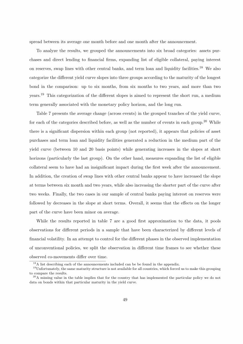
spread between its average one month before and one month after the announcement.

To analyze the results, we grouped the announcements into six broad categories: assets pur-

chases and direct lending to financial firms, expanding list of eligible collateral, paying interest

on reserves, swap lines with other central banks, and term loan and liquidity facilities.18 We also

categorize the different yield curve slopes into three groups according to the maturity of the longest

bond in the comparison: up to six months, from six months to two years, and more than two

years.19 This categorization of the different slopes is aimed to represent the short run, a medium

term generally associated with the monetary policy horizon, and the long run.

Table 7 presents the average change (across events) in the grouped tranches of the yield curve,

for each of the categories described before, as well as the number of events in each group.20 While

there is a significant dispersion within each group (not reported), it appears that policies of asset

purchases and term loan and liquidity facilities generated a reduction in the medium part of the

yield curve (between 10 and 20 basis points) while generating increases in the slopes at short

horizons (particularly the last group). On the other hand, measures expanding the list of eligible

collateral seem to have had an insignificant impact during the first week after the announcement.

In addition, the creation of swap lines with other central banks appear to have increased the slope

at terms between six month and two years, while also increasing the shorter part of the curve after

two weeks. Finally, the two cases in our sample of central banks paying interest on reserves were

followed by decreases in the slope at short terms. Overall, it seems that the effects on the longer

part of the curve have been minor on average.

While the results reported in table 7 are a good first approximation to the data, it pools

observations for different periods in a sample that have been characterized by different levels of

financial volatility. In an attempt to control for the different phases in the observed implementation

of unconventional policies, we split the observation in different time frames to see whether these

observed co-movements differ over time.

18A list describing each of the announcements included can be be found in the appendix.19Unfortunately, the same maturity structure is not available for all countries, which forced us to make this grouping

to compare the results.20A missing value in the table implies that for the country that has implemented the particular policy we do not

data on bonds within that particular maturity in the yield curve.

49

Table 7: Effects of Policies in the Yield Curve and Lending-Deposits spread. Average across events,change in basis points.

Weeks Term Structure Lend. -Measure Type Obs. After Up to 6M 6M to 2Y 2Y+ Dep.

Assets purchases and 12 1 7 -19 -5 4direct lending to financial firms 2 3 -11 -5Expand list of collateral 10 1 1 -1 3 5

2 39 2 1Interest on reserves 2 1 -4 6 20

2 -25 1Swap lines with other CB 6 1 -1 14 4 35

2 22 17 3Term Loan and liquidity 26 1 15 -12 2 12.7Facilities 2 25 -11 2

Note: For the terms structure (columns 4 to 6) the table shows the (average across observa-

tions of the) change in basis point in the slopes between the observation one week before the

announcement of the policy and either one or two weeks after. For the Lending-Deposits spread

(column 7), it is the change (in basis points) of the spread between its average one month before

and one after the announcement.

Table 8 reports the results for three different time frames: before September 2008, between

September and December of 2008, and after January 2009.21 In terms of asset purchases, the

minor reduction in the slope for the first part of the curve observed in the full sample contrasts

with the quite important rise characterizing the three events occurring between September and

December of 2008,22 but for the other nine events the impact on the short part of the curve was

mildly negative.

A similar pattern can be observed for policies that extend the list of eligible collateral. Before

September 2008, these type of announcements where associated with reductions in the slope of the

short part of the yield curve, while after that month this tranche of the slope increased after the

press release. In term of policies introducing term loans and liquidity facilities, it seems that the

21We do not show the results for policies in the group Interest on reserves because the two observations in oursample occurred in the same time frame (between September and December of 2008). The same is true for thecategories missing in the next table.

22These number are mainly driven by the announcement of the Canadian government that it will purchase up to$25 billion in National Housing Act Mortgage-Backed Securities.

50

flattening of the yield curve was more evident when these measures were implemented between

September and December 2008 than after that period.

Table 8: Effects of Policies in Yield Curve and Lending-Deposits spread. Average across events,different time frames, change in basis points.

Time Weeks Term Structure Lend. -Measure type Frame Obs. After Up to 6M 6M to 2Y 2Y+ Dep.

Assets purchases and Before 1 1 -6 4 -3direct lending to financial firms Sep-08 2 -9 5

Sep-08 to 3 1 115 -19 -2 28Dic-08 2 70 -11 0After 8 1 -2 -8 -5Jan-09 2 -1 -8

Expand list of collateral Before 2 1 -9 1 -1 -43Sep-08 2 -13 2 0

Sep-08 to 6 1 5 -6 4 25Dic-08 2 56 2 1After 2 1 3 2 3Jan-09 2 3 1

Swap lines with other CB Sep-08 to 4 1 -1 -6 7 7Dic-08 2 22 3 5After 2 1 33 1 77Jan-09 2 32 1

Term Loan and liquidity Before 1 1 15 6 61Facilities Sep-08 2 5 5

Sep-08 to 19 1 22 -14 3 7Dic-08 2 42 -13 2After 6 1 1 -5 1 29Jan-09 2 0 -6 -1

Another potentially useful split of the sample is based on whether these policies were associated

by different movements depending on whether the rate had already reached its lower bound or not,

which is reported in table 9. While we can see that unconventional policies were mainly implemented

before the central bank chose to drove the policy rate to a low value, some difference can still be

noticed. In terms of policies in the group of asset purchases, it appears that those implemented

after the lower bound was reached had been associated with stronger flattening effects on the yield

curve. On the other hand, the opposite seems to be the case for policies creating term loans and

liquidity facilities.

51

Finally, turning to the behavior of the lending-deposits spread, table 7 shows that, on average,

unconventional measures were followed by increases of this spread. However, looking at the different

time frame decompositions in tables 8 and 9 reveals some exceptions. In particular, assets purchases

seem to have been associated with increases in the spread only in the period between September

2008 and and December 2008. Moreover, there appears to be a marked difference in the observed

behavior of the spread depending on whether the rate was at its lower bound or not. Additionally,

the two announcements of expansions in the list of eligible collaterals implemented before September

2008 (both at the Bank of Canada), were apparently associated with reductions in this spread as

well. Nevertheless, it is worth to mention once again that the frequency of the data on these spreads

is probably not the most adequate to analyze the effects of these types of events.

Table 9: Effects of Policies in Yield Curve and Lending-Deposits spread. Average across events,different time frames, change in basis points.

MPR Weeks Term Structure Lend. -Measure type Bound Obs. After Up to 6M 6M to 2Y 2Y+ Dep.

Assets purchases and Before 4 1 -6 0 36direct lending to financial firms 2 -6 2

After 8 1 11 -19 -9 -142 7 -11 -9

Expand list of collateral Before 9 1 1 -1 3 52 39 2 1

After 1 1 3 02 3 -1

Term Loan and liquidity Before 22 1 21 -14 3 14Facilities 2 36 -14 2

After 4 1 1 7 0 -32 0 6 -2

Overall, it appears that announcements of Assets purchases and direct lending as well as of

Term Loan and liquidity facilities produced a reduction of the slope of the yield curve at medium

horizons; for the other types the evidence is less clear. These effects seem to have been more

marked between September and December 2008 for both of the aforementioned categories. On

the other hand, while the reduction in the slope generated by Assets purchases and direct lending

was apparently stronger after the policy rate reached the lower bound, the impact of Term Loan

52

and liquidity facilities was stronger before reaching the lower bound. In contrast, the effect on the

lending-deposits spread of both types of policies was more pronounced after the lower bound was

attained.

4 Conclusions

Motivated by the numerous unconventional monetary policies that have been implemented during

the current crisis, a new wave of research in monetary policy has been triggered devoted to analyze

the scope and desirability of this heterodox behavior of central banks. Moreover, the discussion

is far from being settled and it will probably keep both theorists and applied economists busy for

years to come.

In this context, the goals of this paper were twofold. On one hand, we provided a theoretical

analysis of the mechanisms that are relevant to understand the effects of these unconventional

policies, and that can be used as a ground for an ex-post evaluation of the measures implemented.

In particular, we first discussed the role of credibility in implementing inflationary goals once the

nominal interest rate is at its lower bound, paying particular attention to the importance of the

central bank’s balance sheet. Additionally, we presented a model which has at its core a financial

imperfection that highlights the role of bank’s capital as well as the relevance of alternative credit

policies that can be used to deal with a situation of financial distress.

On the other hand, we reviewed evidence regarding the recent experience of central banks that

implement inflation target regimes. We first described the timing and the type of unconventional

policies that have been implemented. Second, we explored several alternative measures to asses

the expansivity of monetary policy in a situation when the policy rate has reached its lower bound.

Finally, we presented some descriptive evidence on the effect that the policies implemented had

over two variables that are relevant for the propagation monetary policy: the shape of the yield

curve and the lending-deposit spread.

53

5 References

Banque of France, “Unconventional monetary policy measures,” Focus, April 2009.

Bernanke, B. and V. Reinhart, “Conducting Monetary Policy at Very Low Short-Term Interest

Rates,” American Economic Review, vol. 94(2), May, 2007, 85-90.

Bini Smaghi, L., “Conflicts of Interest and the Financial Crisis,” International Finance, 12:1,

2009, 93-106.

Bundesbank, “Taylor interest rate and Monetary Conditions Index,” Deutsche Bundesbank Monthly

Report, April, 1999.

Christiano, L., R. Motto, and M. Rostagno, “Two Reasons Why Money and Credit May be Useful

in Monetary Policy,” NBER Working Paper No. 13502, October, 2007.

Edwards, S. and C. Vegh, “Banks and macroeconomic disturbances under predetermined exchange

rates,” Journal of Monetary Economics 40(2), 239-278, October 1997.

Eggertsson, G. and M. Woodford, “The Zero Bound on Interest Rates and Optimal Monetary

Policy (with Discussion),” Brookings Papers on Economic Activity, 34(2003-1), 139-235.

Freeman, C., “The Role of Monetary Conditions and the Monetary Conditions Index in the

Conduct of Policy,” Bank of Canada Review Autumn, 1995, 53-60.

Gerlach, S. and F. Smets, “MCIs and monetary policy”, European Economic Review 44 (9),

October 2000, 1677-1700.

Gertler, M., and P. Karadi, “A Model of Unconventional Monetary Policy,” mimeo, 2009, New

York University.

Jeanne, O. and L. Svensson (2007), “Credible Commitment to Optimal Escape from a Liquidity

Trap: The Role of the Balance Sheet of an Independent Central Bank,” American Economic

Review, vol. 97(1), pages 474-490, March

54

Kiyotaki, N. and J. Moore, “Credit Cycles,” Journal of Political Economy 105(2), 211-48, April,

1997.

Krugman, P., “It’s Baaack: Japan’s Slump and the Return of the Liquidity Trap,” Brookings

Papers on Economic Activity 29(2), 1998, 137-206.

Reinhart, V. and B. Sack, “The Economic Consequences of Disappearing Government Debt,”

Brookings Papers on Economic Activity, 2, 2000, 163-220.

Rudebusch, G.D., “The Fed’s Monetary Policy Response to the Current Crisis,” FRBSF Economic

Letter 2009-17, May 22, 2009.

Stevens, G, “Pitfalls in the Use of Monetary Conditions Indexes,” Reserve Bank of Australia

Bulletin, August, 1998, 34-43.

Svensson, L., “The Zero Bound in an Open Economy: A Foolproof Way of Escaping from a

Liquidity Trap,” Monetary and Economic Studies, Institute for Monetary and Economic

Studies, Bank of Japan, vol. 19(S1), 277-312, February, 2001.

Walsh, C., “Optimal Contracts for Central Bankers,” American Economic Review 85 (1995),

150-67.

A Appendix

A.1 Data Sources

Monetary Policy Rates: Central Banks web pages and Bloomberg, daily observations from

Jan2007 to Sep2009 Monthly and quarterly averages were used for calculation purposes

Interest Rates and Yields: IFS, Bloomberg and Central Banks web pages. Lending and

borrowing rates correspond to a monthly average interest rate. Yields corresponds to daily Nominal

Government Bonds (GGR Bloomberg)

55

GDP, CPI and Indusatrial Production:23 The source of this data is the IFS. All sereis are

seasonally adjusted. CPI inflation corresponds to the quarterly annual percentage change in CPI.

GDP gap is a percentage deviation from an HP trend. WTI corresponds to the average West Texas

Intermediate oil price in current USD. RER is the real exchange rate provided by the IFS. NER is

the nominal exchange rate provided by the IFS. CRB is the Commodity Research Bureau/Reuters

US Spot all commodities.

23(*) For Australia, New Zealand and Swizterland we used quarterly data for estimation purposes. Quarterly dataset starts in 1980q1 for Autralia, Canada, Switzerland, Danmark, UK, Japan, Korea, Mexico, Norway, Sweden andUSA. For Brazil the data set starts in 1996q4, for Czech Republic the data set satarts in 1993q1, 1999q1 for the EuroArea, 1985q1 for Hungary, 1995q4 for Peru, 1996q1 for Chile and 1994q1 for Colombia. For all the countries of oursample the data set ends in 2009q1 except for Colombia whose data set ends in 2008q4. For monthly estimationsdata sets start in 1980m1 for: Brazil, Canada, Danemark, UK, Japan, Korea, Norway and USA. For Switzerland thedata set starts in 1995m1 and finishes in 2007m12, for Chile the data set starts in 1987m7, for Mexico in 1981m5,1989m12 for South Africa, 1993m1 for Czech Republic, 1995m3 for Colombia, 1995m10 for Peru, 1999m1 for theEuro Area and 1999m10 for Hungary. All the data sets ends between 2009m5 and 2009m8, except for Switzerlandwhose data set finishes in 2007m12.

56

Time Line of Policy Announcements I

Country Date Measure Type

Australia 24-Sep-08 Domestic term deposit facility Term Loan and/or liquidity Facilities

29-Sep-08 Swap Facility with US Federal Reserve Sawp lines with oher CB08-Oct-08 Expansion of Domestic Market Facilities Term Loan and/or liquidity Facilities06-Nov-08 Domestic Market Dealing Arrangements Term Loan and/or liquidity Facilities

04-Feb-09 Reserve Bank of Australia and US Federal Reserve Swap Facility Sawp lines with oher CB

02-Mar-09 Domestic Market Dealing Arrangements Term Loan and/or liquidity Facilities

Canada 15-Ago-07Temporarily Expands List of Collateral Eligible for SPRA Transactions

Expand/or list of collaterals

31-Mar-08Accepting Asset-backed Commercial Paper (ABCP) as Collateral for the Bank of Canada's Standing Liquidity Facility (SLF)

Expand/or list of collaterals

10-Oct-08The federal government announced that it will purchase up to $25 billion in National Housing Act Mortgage-Backed Securities

Assets purchase and/or Direct lending to financial firms

Chile 29-Sep-08Reserve accumulation program was terminated, USD repo 1 month operations announced (sales of USD spot + 1 month forward USD purchases, through competitive auctions)

Term Loan and/or liquidity Facilities

10-Oct-08Broadening of eligible collaterals for money market operations(now encompassing CDs), USD repo program extended to six months.

Expand/or list of collaterals

10-Dic-08 Extension of liquidity measures for all of 2009. Term Loan and/or liquidity FacilitiesEnhancement of liquidity facility through credit lines accepting a broader range of collateral for longer tenors.

Expand/or list of collaterals

09-Jul-09MPR at lower bound, short term liquidity facility, suspension of debt emision of long maturities

Term Loan and/or liquidity Facilities

Euro 26-Sep-08Measures designed to address elevated pressures in the short-term US dollar funding markets,

Term Loan and/or liquidity Facilities

29-Sep-08 Conduct of a special term refinancing operation Term Loan and/or liquidity Facilities07-Oct-08 US dollar liquidity-providing operations Term Loan and/or liquidity Facilities18-Dic-08 Tender procedures and the standing facilities corridor Term Loan and/or liquidity Facilities06-Abr-09 Central banks announce expanded swap arrangements Sawp lines with oher CB

07-May-09Longer-term refinancing operations. ECB decided to enhance its set of non-standard measures

Term Loan and/or liquidity Facilities

04-Jun-09 Coverded bonds Purchases of 60 billion Euro Others08-Jul-09 EIB(European Investment Bank) an elligible counterparty Expand/or list of collaterals

Japan 14-Oct-08Increase in the frequency and size of repo operations. Steps to Facilitate Corporate Financing

Others

31-Oct-08 Introduction of lending facilities Term Loan and/or liquidity FacilitiesKorea 27-Oct-08 Increased of agg credit. Remuneration of reserves Interest on reserves

08-Nov-08 Broadening eligible collaterals for OMOs Expand/or list of collateralsLiquidity provisions to financial institutions Term Loan and/or liquidity Facilities

New Zealand 12-Oct-08 Deposit guarantee scheme introduced Others29-Oct-08 RBNZ, Federal Reserve announce USD facility Term Loan and/or liquidity Facilities07-Nov-08 Reserve Bank announces new facilities Term Loan and/or liquidity Facilities12-Dic-08 Reserve Bank announces further liquidity measures Term Loan and/or liquidity Facilities

13-Ene-09 Tuesday OMO to accept Corporate and Asset Backed securities Expand/or list of collaterals

Norway 24-Sep-08Central banks announce expanded swap facilities with U.S. Federal Reserve

Sawp lines with oher CB

12-Oct-08 Two-year F-loan for small banks Term Loan and/or liquidity Facilities29-Oct-08 Easing collateral requirements Expand/or list of collaterals

57

Time Line of Policy Announcements II

Country Date Measure Type

Sweden 22-Sep-08 Press Release: Changed collateral requirements for credit in RIX Expand/or list of collaterals

24-Sep-08Central Banks Announce Swap Facilities with U.S. Federal Reserve

Sawp lines with oher CB

29-Sep-08 Riksbank announces new swap facility in US dollars Term Loan and/or liquidity Facilities02-Oct-08 Riksbank lends SEK 60 billion over three months Term Loan and/or liquidity Facilities06-Oct-08 Increased loans and longer maturity Term Loan and/or liquidity Facilities08-Oct-08 Changed collateral requirement for credit in RIX Expand/or list of collaterals

Switzerland 26-Sep-08Measures taken by central banks to calm the money markets 30 bn swap line with the FED to p´rovide USD in Swiss market

Sawp lines with oher CB

29-Sep-08USD swap line with the U.S. Federal Reserve increased, Swap line expanded to 60 bn and until April 2009

Sawp lines with oher CB

15-Oct-08Swiss National Bank and European Central Bank cooperate to provide Swiss franc liquidity

Term Loan and/or liquidity Facilities

16-Oct-08Steps to strengthen the Swiss financial system.SNB finances transfers of UBS illiquid assets

Assets purchase and/or Direct lending to financial firms

18-Dic-08 SNB StabFund acquires first tranche of assets from UBSAssets purchase and/or Direct lending to

financial firms

25-Jun-09Swiss National Bank continues to provide Swiss francs through EUR/CHF foreign exchange swaps

Term Loan and/or liquidity Facilities

England 19-Ene-09BoE announces GBP 50 billion in purchases of high-quality private sector assets

Assets purchase and/or Direct lending to financial firms

09-Abr-09BoE reduces bank rate to 0.5% and continues APF with £75 Billion

Assets purchase and/or Direct lending to financial firms

07-May-09BoE maintains Bank Rate at 0.5% and Increases Size of Asset Purchase Programme by £50 Billion to £125 Billion

Assets purchase and/or Direct lending to financial firms

04-Jun-09BoE Maintains Bank Rate at 0.5% and continues with £125 Billion Asset Purchase Programme

Assets purchase and/or Direct lending to financial firms

08-Jun-09Asset purchase to be expanded to includesecured commercial papers

Assets purchase and/or Direct lending to financial firms

09-Jul-09BoE Maintains Bank Rate at 0.5% and continues with £125 Billion Asset Purchase Programme

Assets purchase and/or Direct lending to financial firms

06-Ago-09BoE Maintains Bank Rate at 0.5% and Increases. Size of Asset Purchase Programme by £50 Billion to £175 Billion

Assets purchase and/or Direct lending to financial firms

10-Sep-09 BoE Maintains Bank Rate at 0.5% and continues, with £175 Billion Asset Purchase Programme

Assets purchase and/or Direct lending to financial firms

United States 21-Dic-07 Federal Reserve intends to continue TAF auctions as necessary Term Loan and/or liquidity Facilities

13-Jul-08Lending to Fannie Mae and Freddie Mac at the primary credit rate is autorized

Assets purchase and/or Direct lending to financial firms

19-Sep-08 AMFL or "the facility" established Term Loan and/or liquidity Facilities

06-Oct-08FED will begin to pay interest on depository institutions' required and excess reserve balances and Increase of TAF

Interest on reserves

02-Dic-08

Extension through April 30, 2009, of three liquidity facilities: the Primary Dealer Credit Facility (PDCF), the Asset-Backed Commercial Paper Money Market Fund Liquidity Facility (AMLF), and the Term Securities Lending Facility (TSLF)

Term Loan and/or liquidity Facilities

10-Feb-09Expanding TALF and accept wider set of collateral (FED states willingness to expand TALF to $1 trillion)

Term Loan and/or liquidity Facilities

18-Mar-09

FED increases balance sheets by purchasing further 750 billions of asset backet-securities from agencies bringing this year total purchases up to 1.25 trillions. Announcement of program to buy $300b worth of Treasury securities.

Assets purchase and/or Direct lending to financial firms

25-Jun-09 Extension of Liquidity Facilities and Swap lines Term Loan and/or liquidity Facilities

58