heterogeneous impacts of domestic outsourcing on wages ... · heterogeneous impacts of domestic...

Heterogeneous impacts of domestic outsourcing on wages

Carlos Alberto Belchior (PUC-Rio)

Geovana Lorena Bertussi (UnB)

Abstract: This paper assesses the consequences of domestic outsourcing on different groups of workers,

stemming from a theoretical model with heterogeneous individuals and firms. We find the wage gap

between outsourced workers and non-outsourced ones to be larger for more productive workers, as well

as for those who work at sectors where observation of their effort is harder. Furthermore, using Brazilian

micro-data and quantile regressions, we demonstrate that the effect of outsourcing on wages grows with

income, as suggested by the theoretical model.

Key words: outsourcing, efficiency wage, quantile regression.

JEL classifications: J31, C21.

Resumo: Este artigo avalia as consequências da terceirização doméstica sobre diferentes grupos de

trabalhadores a partir de um modelo teórico com indivíduos e firmas heterogêneos. Nossa análise teórica

indica que o gap salarial para trabalhadores terceirizados deve ser maior para os trabalhadores mais

produtivos, assim como para aqueles indivíduos que trabalham em setores em que é mais difícil observar

o seu esforço. Além disso, usando microdados brasileiros, nós evidenciamos por meio de um arcabouço

de regressão quantílica que os efeitos da terceirização sobre os salários tornam-se mais relevantes para os

indivíduos com maior salário, o que corrobora as conclusões do nosso modelo teórico.

Palavras-Chave: terceirização, salário eficiência, regressão quantílica.

Classificação JEL: J31, C21.

Área de submissão: Economia do trabalho

1. Introduction

Over the last two decades, the economic impacts of service outsourcing have generated ever-

increasing academic interest (MANKIW and SWAGEL, 2006). Amid these studies (carefully reviewed in

the next section), some seek to estimate outsourcing’s effects on wages, and overall conclude that

outsourced workers earn less than their non-outsourced counterparts.

Williamson (2008) suggests the outsourcing processes can be adopted under very distinct

circumstances and with equally distinguished objectives. Thus, workers from different sectors and levels

of human capital could be outsourced.

In this paper, we focus on domestic outsourcing – witch contrasts with offshoring

(GOLDSHIMIDT and SCHMIEDER, 2017). We evaluate whether the effects of outsourcing on workers’

wages are homogeneous or not. We therefore intend to build a highly stylized model that underlines how

disparities in the labor outsourcing sector and in the outsourced workers’ productivity can influence the

observed wage gap.

Moreover, an empirical analysis will be carried in order to test the conclusions of this theoretical

model. Data from the Annual Social Information Report (RAIS) for 2014 will be used, and so will a

methodology of quantile regression, to explore heterogeneous effects of outsourcing on wages.

This article consists of five sections, in addition to this introduction. Section 2 reviews literature

concerning outsourcing in relation to wages. Section 3 develops the theoretical model. Section 4 discusses

the database employed, as well as presents the empirical model and its results. Section 5 tests the

adjustment of the model when we control for selection of outsourced workers.

2. The impact of outsourcing on wages

As pointed out in the introduction, this paper focuses on domestic outsourcing processes and their

implications on the wages of the workers who have been outsourced. Berlinski (2008) is the first paper

with similar purpose. He assess the consequences of outsourcing for low human capital workers in the

United Kingdom.

The author builds a database for workers from 1995 to 2001 and conducts estimates of a

Mincerian equation, which includes a dummy variable for outsourced workers, through Generalized Least

Squares (GLS) and propensity score matching, and concludes that the evaluated workers are paid 17% to

19% less than non-outsourced similar employees. His outsourcing definition is somewhat limited, since

his database has fewer than sixty outsourced workers.

Dube and Kaplan (2010) also perform an empirical work to analyze the effect of outsourcing on

low-human capital workers, more specifically guards and janitors, in the U.S. An outsourcing indicating

variable, similar to the one used in this study, is created by the combination of information on the job

performed by each worker and the sector in which they work, using micro-data from the Current

Population Survey (CPS), between 1983 and 2000.

The authors construct a Mincerian equation and estimate it via the Generalized Least Squares

(GLS) method. In this first estimation, it is shown that outsourced janitors make about 5% less, while

guards earn about 20% less, when compared to non-outsourced workers in the same occupation.

Dube and Kaplan (2010) then examine if unobservable differences in productivity may explain the

wage gap. They build a two-period panel and individuals with the same occupation are observed on each

of the periods. Subsequently, a new wage equation is estimated through the first difference method. The

outsourcing wage penalties still remain though, around 7% for janitors and 12% for guards. This

methodology was, then, used in all subsequent papers on the topic.

Thereby, the authors find outsourced workers are paid less due to their contract type. They also

conclude that the penalty suffered by the workers is not explained by low rent pass-through or

compensating differentials, so it must be associated with some non-taken rent, like the one obtained

through unionization, for instance; since the persistent estimated difference is not compatible with the

hypothesis of a competitive market. Despite these considerations, Dube and Kaplan (2010) do not go

further in the outsourcing wage penalty theory.

Stein, Zylberstajn e Zylberstajn (2016) apply the previous methodology to Brazilian data. The

authors consider outsourced workers in the cleaning, security, technology of information (TI),

maintenance and research and development (R&D). The author show that almost all the raw outsourced

wage gap in their sample can be explained by different individual characteristics. Once they control for

variant observable and fixed unobservable characteristics through the first-difference method, they

conclude that the average wage gap is about only 3%.

They do not systematically analyze how the wage gap varies with different characteristics of the

workers, but, by estimating separate regressions for each sector, they point out that the gap tends to be

higher for low-skilled workers.

Belchior and Bertussi (2016) also utilize a Brazilian data, similar to the one in this paper, and

used the detailed available classifications on occupations and sectors in order to create broad

classification for outsourced workers1. A Mincerian equation is estimated, in order to conclude that

outsourced workers earn 7.2% to 10.5% less than non-outsourced ones. Furthermore, the authors examine

if unobservable fixed effects bias the estimate, in a similar manner as Dube and Kaplan (2010); then,

through a first difference model in panel data, come to the conclusion that a fixed bias does not

significantly alter the previous estimation. An extensive analysis is carried, looking to identify average

effects of outsourcing.

The authors argue that these wage disparities are motivated by differences in efficiency wage

payments for outsourced and non-outsourced workers. This suggestion provides an explanation for the

difference in rents uncovered by Dube and Kaplan (2010).

Goldshimidt e Schmieder (2017) also employed the previous methodology and estimated average

impacts of outsourcing on German workers of logistics, food, security and cleaning (LFSC) sectors. They

found that analyzed outsourced workers suffered a 9% wage penalty. These results are broadly consistent

with previous estimates.

Despite that, they argue that it is difficult to account for different job characteristics of outsourced

workers. The authors suggest using on-site outsourcing events as an identification strategy. They identify

several aggregate flows of workers from final to intermediate firms in the LFSC’s sectors. It is argued

that these outsourced workers were likely to perform the same activities as they were previously doing.

Their estimates show that the workers who passed through such an event received between 10%

and 15% less than similar workers who were not outsourced, ten years of the outsourcing event.

Goldshimidt e Schmieder (2017) also employ the decomposition methodology employed by Card,

Heining e Kline (2013) and conclude that differences in firm’s rents explained all the declining relative

wages of outsourced workers.

So, the previous studies consistently estimated negative average impacts of outsourcing on

workers’ wages and associated then with differences in non-competitive rents captured by those workers,

relying mostly on fixed-effect estimates. These conclusions are congruent with recent empirical findings,

derived from the works of Abowd, Kramarz and Margolis (1999), Card, Heining and Kline (2013) and

Song et al. (2016).

Song et al. (2016), in particular, decomposed the variance of income and concluded that the most

important fraction in the increased country inequality (more than two-thirds) is attributed to the increased

inequality between firms, and not between workers in the same firm. Further yet, they show this process

is mostly due to a larger segregation of workers in different companies.

They suggest outsourcing may be a relevant factor in explaining this process. However, they claim

that simply dividing workers into more and less productive would not alter income distribution if they

were paid in equivalence to their marginal productivity in both cases. In these terms, the uncovered

difference in rents by difference outsource workers may help explaining these patterns in wage inequality.

This paper further explores the previous insights in mainly two dimensions. First, we develop a

concrete theoretical explanation for the difference in rents appropriated by workers. Second, we

systematically explore how outsourcing effects varies both theoretically and empirically for different

workers.

1 The work considers as outsourcing any type of service related to production and transferred to a third party. Thus, the

database includes workers on different levels of human capital. For example, it considers consulting as a type of outsourcing.

3. Theoretical model

In this section, first Belchior and Bertussi (2016)’s model will be replicated, and then it will be

expanded in order to incorporate more than one individual, as well as different sectors.

3.1 Base model

The economy under consideration has n identical workers whose preferences are represented by

the utility function:

𝑢 = 𝑤 − 휀 (1)

where 𝑤 is the wage perceived by the workers and 휀 indicates their level of effort. We will assume that

the worker can perform on two levels of effort – high and low. The variable 휀 will assume value 1 if the

worker performs on high effort, and value 0 if they perform on low effort.

Workers receive unemployment insurance of value �̅� if they are not working, which acts as a

reservation wage. Their effort is not perfectly observable. In case the effort is not being made, the

employer observes this behavior with a probability of 𝑝. If the workers are caught shirking, they are fired.

The benefits are evaluated by the workers according to the expected utility theory. If they perform

with high effort, 휀 assumes value 1, so they will not be submitted to uncertainty and their utility will be:

𝑢𝑒 = 𝑤 − 1 (2)

Conversely, if they show low effort their utility will be:

𝑢𝑛 = 𝑤 ∗ 𝑝 + (1 − 𝑝) ∗ 𝑤 (3)

This way, it can be assured that the workers will exert effort if, and only if:

𝑤 ≥ 𝑤 +

1

𝑝

(4)

We shall assume the economy contains only one final good, produced by m identical firms

operating under perfect competition and with the objective function given by:

𝜋 = (1 + 𝛿휀) ∗ 𝑆(𝑛) − (𝐶 + 𝑤) ∗ 𝑛, 𝛿 > 0 (5)

where 𝑆(𝑛) is a strictly concave revenue function for the firms, 𝑛 is the amount of workers hired and 𝐶

represents costs associated to labor management (social charges, labor management costs, etc). It can be

noted that when the workers make an effort (so that 휀 assumes a value of 1) the firms’ revenue function is

moved up by a positive factor (1 + 𝛿), where 𝛿 is the increment factor of the revenue curve by effort.

It helps to define the derivative of the inverse revenue function as:

𝑆′(𝑛)−1 = 𝜑(𝑛) (6)

One can easily understand that firms can maximize their profits in distinct states of nature, paying

the efficiency wage or not. A firm may determine:

max𝑛

𝜋 = 𝑆(𝑛) − (𝐶 + 𝑤) ∗ 𝑛 (7)

𝑠. 𝑎 𝑤 ≥ �̅�

in such a way as to not encourage workers to make an effort. In this case, we have:

𝑛 = 𝜑(𝐶 + �̅�) (8)

When the firm pays high enough salaries to induce workers to exert effort (so that 휀 assumes the

value of 1), it will determine:

max𝑛𝑒

𝜋𝑒 = (1 + 𝛿) ∗ 𝑆(𝑛𝑒) − (𝐶 + 𝑤) ∗ 𝑛𝑒

(9)

𝑠. 𝑎 𝑤 ≥ �̅� +1

𝑝

Optimally, we have:

𝑛𝑒 = 𝜑 (𝐶 + �̅� +

1𝑝

1 + 𝛿)

(10)

If the shift in productivity is big enough, it will compensate the increase in wage costs, and firms will opt

for paying the efficiency wage.

Now, an additional firm2 that provides outsourced labor to the firms producing the final good is

introduced. It is assumed to be more efficient than others in executing labor management, without

incurring cost 𝐶. Additionally, said cost is supposed to be reduced to zero, in order to facilitate further

mathematical development on the model.

The outsourcing firm pays a high enough wage to attract the workforce, and then passes it on to

the other companies for a value 𝑤𝑜, in a similar outsourced labor supply model to the one proposed by

Holmes e Snider (2011). It will receive unitary profit:

𝑤𝑜 − 𝑤 > 0 (11)

An important point is that labor outsourcing firms have no incentive for paying the efficiency

wage, since they cannot benefit directly from the increase in labor productivity, and it raises costs.

Now, firms can maximize their profit in three different states of nature, including the one where

they hire outsourced labor:

max𝑛𝑡

𝜋 = 𝑆(𝑛𝑡) − 𝑤𝑜 ∗ 𝑛𝑡 (12)

which gives us, optimally,

𝑛𝑡 = 𝜑(𝑤𝑜) (13)

As with the efficiency wage case, the referred paper denotes that, for a sufficiently large cost

reduction, the contracting of outsourced labor increases the profitability of firms. It also reduces the wage

and productivity of workers, since they are not encouraged to deliver a high level of effort through the

efficiency wage payment.

2 The hypothesis that outsourcing firms operate as a monopoly is consistent with the work of Baccara (2007).

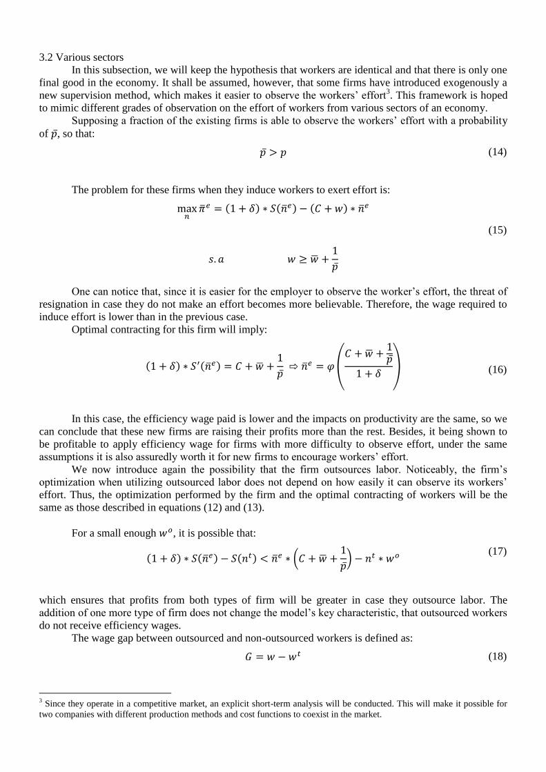
3.2 Various sectors

In this subsection, we will keep the hypothesis that workers are identical and that there is only one

final good in the economy. It shall be assumed, however, that some firms have introduced exogenously a

new supervision method, which makes it easier to observe the workers’ effort3. This framework is hoped

to mimic different grades of observation on the effort of workers from various sectors of an economy.

Supposing a fraction of the existing firms is able to observe the workers’ effort with a probability

of �̅�, so that:

�̅� > 𝑝 (14)

The problem for these firms when they induce workers to exert effort is:

max𝑛

�̅�𝑒 = (1 + 𝛿) ∗ 𝑆(�̅�𝑒) − (𝐶 + 𝑤) ∗ �̅�𝑒

(15)

𝑠. 𝑎 𝑤 ≥ �̅� +1

�̅�

One can notice that, since it is easier for the employer to observe the worker’s effort, the threat of

resignation in case they do not make an effort becomes more believable. Therefore, the wage required to

induce effort is lower than in the previous case.

Optimal contracting for this firm will imply:

(1 + 𝛿) ∗ 𝑆′(�̅�𝑒) = 𝐶 + �̅� +1

�̅� ⇨ �̅�𝑒 = 𝜑 (

𝐶 + �̅� +1�̅�

1 + 𝛿)

(16)

In this case, the efficiency wage paid is lower and the impacts on productivity are the same, so we

can conclude that these new firms are raising their profits more than the rest. Besides, it being shown to

be profitable to apply efficiency wage for firms with more difficulty to observe effort, under the same

assumptions it is also assuredly worth it for new firms to encourage workers’ effort.

We now introduce again the possibility that the firm outsources labor. Noticeably, the firm’s

optimization when utilizing outsourced labor does not depend on how easily it can observe its workers’

effort. Thus, the optimization performed by the firm and the optimal contracting of workers will be the

same as those described in equations (12) and (13).

For a small enough 𝑤𝑜, it is possible that:

(1 + 𝛿) ∗ 𝑆(�̅�𝑒) − 𝑆(𝑛𝑡) < �̅�𝑒 ∗ (𝐶 + �̅� +

1

�̅�) − 𝑛𝑡 ∗ 𝑤𝑜

(17)

which ensures that profits from both types of firm will be greater in case they outsource labor. The

addition of one more type of firm does not change the model’s key characteristic, that outsourced workers

do not receive efficiency wages.

The wage gap between outsourced and non-outsourced workers is defined as:

𝐺 = 𝑤 − 𝑤𝑡 (18)

3 Since they operate in a competitive market, an explicit short-term analysis will be conducted. This will make it possible for

two companies with different production methods and cost functions to coexist in the market.

where 𝑤𝑡 is the wage received by the outsourced workers. In the case of the original firms, the gap is:

𝐺 =

1

𝑝

(19)

As for the ones with the new supervision method, the wage gap is given by:

�̅� =

1

�̅�

(20)

From that, given the restriction imposed by equation (14), we can guarantee that:

1

�̅�<

1

𝑝 ⇨ �̅� < 𝐺

(21)

From this framework, one can observe a negative relationship between the increase in probability

of detecting lack of effort in a sector and the wage gap in that same sector.

3.3 Various individuals

In this subsection, we go back to envisioning only one type of firm in the economy. Additionally,

one more type of worker is brought in to the analysis. We shall now assume there is a fraction of high-

skilled workers in this economy. These workers, as well as the low-skilled ones, can execute a high or

low level of effort. Nevertheless, they will be assumed to be more productive and to bring a higher return

rate for the firm from their effort. This will be inserted in the model, and 휀 will now assume values 1 and

2.

Such modeling allows productivity disparities of workers to be added to the model. Note that the

individual incurs costs (in this case, higher effort) to increase their productivity, in a similar way to

investment in human capital by individuals4.

The firm is assumed to be capable of distinguishing high-skilled from low-skilled workers (those

able to execute higher effort and be more productive, and those less able to do that). Nonetheless, it still

cannot perfectly observe the level of effort achieved by individuals. So, it will observe with a probability

of p whether a high-skilled individual is showing low effort (so that 휀 = 1) and dismiss them if that is the

case.

When high-skilled individuals do not make an effort, their well-being is given by:

𝑢𝑞𝑛 = 𝑤 ∗ 𝑝 + (1 − 𝑝) ∗ (𝑤𝑞 − 1) (22)

and, when they do:

𝑢𝑞𝑒 = 𝑤𝑞 − 2 (23)

where subscript q indicates a reference to high-skilled workers.

Workers will exert effort if:

𝑢𝑞

𝑒 ≥ 𝑢𝑞𝑛 ⇨ 𝑤𝑞 ≥ �̅� +

1

𝑝+ 1

(24)

4 Despite the resemblance, we opted for not making the decision of investment in human capital endogenous, in order to keep

the simplicity of the model.

Evidently, the required wage for high-skilled workers to exert effort is higher than the one

required for the low-skilled, as stated in equation (4). This fits the empirical observation that high-skilled

workers have a higher reservation wage (KRUEGER and MUELLER, 2016).

The new objective function for the firms is:

𝜋 = (1 + 𝛿휀𝑛𝑞) ∗ 𝑆(𝑛𝑛𝑞) + (1 + 𝛿휀𝑞) ∗ 𝑆(𝑛𝑞) − (𝐶 + 𝑤𝑛𝑞) ∗ 𝑛𝑛𝑞 − (𝐶 + 𝑤𝑞) ∗ 𝑛𝑞 (25)

where subscript 𝑛𝑞 indicates a reference to low-skilled workers.

Supposing that

(1 + 2𝛿) ∗ 𝑆(𝑛𝑞

𝑒) − (1 + 𝛿) ∗ 𝑆(𝑛𝑞) > (𝐶 + �̅�) ∗ (𝑛𝑞𝑒 − 𝑛𝑞) + 𝑛𝑞

𝑒 +𝑛𝑞

𝑒

𝑝

(26)

is valid, it is ensured the firm will also pay efficiency wage to high-skilled workers. Therefore, the

problem for firms is:

max𝑛𝑞

𝑒 ,𝑛𝑛𝑞𝑒

𝜋 =(1 + 𝛿휀𝑛𝑞) ∗ 𝑆(𝑛𝑛𝑞) + (1 + 𝛿휀𝑞) ∗ 𝑆(𝑛𝑞) − (𝐶 + 𝑤𝑛𝑞) ∗ 𝑛𝑛𝑞 − (𝐶 + 𝑤𝑞) ∗ 𝑛𝑞

(27)

𝑠. 𝑎 𝑤𝑛𝑞 ≥ �̅� +1

𝑝

𝑤𝑞 ≥ �̅� +1

𝑝+ 1

The solving of the firm maximization problem yields:

𝑆′(𝑛𝑞𝑒) ∗ (1 + 2𝛿) = �̅� +

1

𝑝+ 1 ⇨ 𝑛𝑞

𝑒 = 𝜑 (𝐶 + �̅� +

1𝑝 + 1

1 + 2𝛿)

(28)

The optimal choice for low-skilled workers, in turn, is similar to the one obtained in equation (10).

More productive workers receive higher wages than their low-skilled peers. In the model, this occurs

because effort is more costly for productive individuals, and employers are willing to pay a higher wage

in exchange for a bigger effort from them.

Now, the possibility of labor outsourcing by the firms will be introduced one more time, under the

terms of the previous subsections. A firm that outsources labor has access both to high-skilled and low-

skilled labor. It pays reservation wages to every type of individual, but renders its services to the firm

producing the final good at distinct prices, so that high-skilled labor costs more than low-skilled labor.

Keeping the premises from previous subsections and assuming that

(1 + 2𝛿) ∗ 𝑆(𝑛𝑞

𝑒) − (1 + 𝛿) ∗ 𝑆(𝑛𝑞𝑡 ) < 𝑛𝑞

𝑒 ∗ (𝐶 + �̅� +1

𝑝+ 1)−𝑛𝑞

𝑡 ∗ 𝑤𝑞𝑜

(29)

where 𝑤𝑞𝑜 represents the price of rendering high-skilled service to firms that produce the final good, we

can assure the outsourcing of high-skilled workers is also efficient for firms.

Thus, the firm making the final good determines:

max𝑛𝑞

𝑡 ,𝑛𝑛𝑞𝑡

𝜋 = 𝑆(𝑛𝑛𝑞𝑡 ) + (1 + 𝛿) ∗ 𝑆(𝑛𝑞

𝑡 ) − 𝑤𝑞𝑜 ∗ 𝑛𝑞

𝑡 + 𝑤𝑛𝑞𝑜 𝑛𝑛𝑞

𝑡 (30)

which gives:

𝑆′(𝑛𝑞

𝑡 ) ∗ (1 + 𝛿) = 𝑤𝑞𝑜 ⇨ 𝑛𝑞

𝑡 = 𝜑 (𝑤𝑞

𝑜

1 + 𝛿)

(31)

The optimal amount of low-skilled outsourced workers hired is similar to that obtained in equation

(13).

By using the definition of wage gap, specified in equation (18), we find the gap for low-skilled

workers to be identical to the one shown in equation (19). On the other hand, for high-skilled workers,

𝐺𝑞 =

1

𝑝+ 1

(32)

infers that

1

𝑝+ 1 >

1

𝑝⇨ 𝐺𝑞 > 𝐺𝑛𝑞

(33)

We therefore conclude that the gap between outsourced and non-outsourced workers must be

larger for high-skilled individuals than for low-skilled individuals.

4. Empirical analysis

Our model yields two clear empirical predictions. First, we expect that the wage gap of outsourced

workers will be higher for more productive workers - witch contradicts some of the insights provided by

previous papers. Second, our model predicts that the gap will be greater in sectors where it is difficult to

observe effort.

In the following sections we will analyze only the first empirical prediction of our theoretical

model. As will be discussed in subsection 4.2, we can use occupation and sector detailed classifications to

identify which workers are outsourced, but we frequently cannot tell which final firms effectively employ

the worker. This prevents us from testing the second prediction above.

4.1 Econometric model

Seeking to test the model’s predictions, the following mincer equation will be estimated first:

ln(𝑤𝑖) = 𝛼𝑇𝑖 + 𝑿𝒊𝜷 + 𝑢𝑖 (34)

We take the natural logarithm of the wage of individual i (𝑤𝑖) as function of a variable that

indicates whether the worker is outsourced (𝑇𝑖) and a vector of control variables (𝑿𝒊). We wish to assess

whether outsourced workers earn less, once relevant cofactors are controlled, such as the previously

reviewed empirical studies did.

Next, the quantile regression framework will be used to examine wage distribution among

individuals, conditional to outsourcing and other cofactors in several quantiles of earning distribution.

Let:

ln(𝑤𝑖) = 𝑦𝑖 (35)

and

𝛼𝑇𝑖 + 𝜷𝑿𝒊 = 𝒛𝒊 (36)

Formally, the quantile regression will be estimated by:

min𝜷,𝜶

∑ 𝜃 ∗ |ln(𝑤𝑖) − 𝛼𝑇𝑖 − 𝜷𝑿𝒊| + ∑ (1 − 𝜃) ∗ |ln(𝑤𝑖) − 𝛼𝑇𝑖 − 𝜷𝑿𝒊|

𝑖:𝑦≤𝑧𝑖:𝑦≥𝑧

(37)

where 𝜃 indicates the quantile of analysis. We obtain a coefficient vector that minimizes the equation in

the desired quantiles and corresponds to the conditional mean of the variables of interest in the quantile 𝜃

(KOENKER and BASSET, 1978; KOENKER and HALLOCK, 2001). This analysis will allow a very

detailed decomposition of how outsourcing affects the wages of workers with different productivities.

This has not been achieved yet, in any Brazilian or international study.

4.2 Database

We will employ micro-data from the Annual Social Information Report (RAIS) for 2014. This

data is annually reported for nearly all formal firms in Brazil and used it is used for social security

purposes. The misreport of information is subject to penalty, so most firms use specialist accountants to

register the information (ALVAREZ et al, 2017).

RAIS contains information on several demographical characteristics of individuals and some

characteristics of the firm in which he is employed. Despite that, the database does not divide the

information for outsourced and non-outsourced workers. In order to overcome this issue, we use the

method suggested by Dube e Kaplan (2010) for the CPS in the U.S.

Said method has been proposed by Belchior e Bertussi (2016) and consists of cross-linking data

from the Brazilian Classification of Occupations (CBO) and the National Classification of Economic

Activity (CNAE). They take advantage of the specificity of those classifications and identify outsourced

workers in a very broad selection of sectors.

Also, we will use a identified version of the database, provided by the Work and Employment

Ministry (MTE) for the purpose of research. This particular version of the database contains information

that allow us to identify firms and individuals across time.

Thereby, we will initially be working with about 50 million observations in the database, the size

of the Brazilian formal sector. Nonetheless, we could not use it entirely, as the estimation of the quantile

regression (described in the last subsection) becomes computationally unfeasible with that number of

observations. In order to solve this problem, we created a random sub-sample with 250 thousand

observations5 from the original database. The process to attain this sub-sample is described in Appendix

II.

4.3 Description of the Variables

Our dependent variable is the natural logarithm of employee remuneration in December 20146. In

opposition to prior estimates, which used the average workers’ remuneration along the year, we chose to

use just the remuneration for the last month of the year. That is because the statements that compose the

database are given by employers, and they tend to fill in recent information more accurately (RAMOS,

2012).

5 Once it became evident that the quantile regression estimation would not be feasible with the full sample, we created several

random samples with reduced number of observations. Starting with one million, we progressively diminished the sample until

it became estimable, at a number of 250 thousand observations. We performed the regressions on Table 1 with our random

sub-sample, and results were very similar to those found using the entire database. Besides, as will be detailed in the next

section, this sub-sample is large enough to make sure all the estimated coefficients are significant to the level of 1% in any of

the quantiles. 6 Workers who were dismissed throughout the year were excluded from the sample.

The control vector is formed by the following variables: education; age (on level and squared);

experience in the firm the worker is employed at (on level and squared); geographic region they live in;

sector they work in; gender; ethnicity; and size of reported establishment.

The education variable, measured by the maximum level of instruction achieved, aims to control

the individuals’ difference in productivity7. According to human capital theory, prevalent in the

explanation of individuals’ varying remunerations, this should be a very relevant factor to the observed

wage variation (BECKER, 1975).

The adding of age and experience at current job variables, used as proxy for the individual’s

experience in the work market, seeks to identify the presence of specific human capital, acquired with

time in the job. A quadratic term was included to detect non-linear relationships within the experience-

wage relation, since the productivity gains generated are exhausted over time (ARROW, 1962). The

variables are measured in months and point to how long the individual has worked for the same company.

Binary variables are added to control regional segmentations in wage determination or

discrimination patterns against minorities. The Northeast region was taken as reference and dummy

variables were assigned for the other regions. The ethnicity binary variable assumes value 1 if the

individual is white, and value 0 if they belong to any other ethnic group. We also used a binary variable to

identify outsourced and non-outsourced workers, according to the classification discussed in the last

subsection.

At last, we added establishment size to the regression as an indicator for the propensity of the

individual to receive an efficiency wage (OI and IDSON, 1999). The size of the company is defined by

the number of workers, according to the rating recommended by SEBRAE (2013) when using data from

RAIS8.

4.4 Results

In Table 1, an estimation of equation (34) is performed. In model (1), we only perform the

regression of the wage logarithm’s variable as a function of the outsourcing dummy variable. In model

(2), are included in the regression controls of education, experience (on level and squared) and age –

consistent with human capital theory, without discrimination or segmentation in the labor market.

Ultimately, in model (3) all aforementioned variables are included.

Table 1 – Results of the Mincerian Regression (34) through GLS

Note: The statistic significance of the estimated coefficient is indicated by the number of asterisks: * indicates 10%

significance, ** indicates 5% significance and *** indicates 1% significance.

One can observe that, in all models, the control variable coefficient presents the sign expected by

literature. Moreover, all of them present statistic significance of 1%.

7 Levels of instruction are: incomplete primary school, complete primary school, incomplete secondary school, complete

secondary school, incomplete superior education, complete superior education, master’s degree, doctoral degree. 8 Our variable assumes four levels: Microenterprise (up to 9 employees), small enterprise (10 to 49 employees), medium

enterprise (50 to 99 employees) and big enterprise (more than 100 employees).

Variable Coefficient Standard Error Coefficient Standard Error Coefficient Standard Error

Outsourced -0.297*** 0.0004 -0.130*** 0.0003 -0.136*** 0.00042

Education - - 0.185*** 0.00005 0.165*** 0.00006

Experience - - 0.0039*** 0.00000 0.0033*** 0.00000

Experience2

- - -0.00004*** 0.00000 -0.00003*** 0.00000

Age - - -0.0084*** 0.00000 0.0089*** 0.00001

Firm size - - - - 0.116*** 0.00008

Male - - - - 0.250*** 0.00019

White - - - - 0.076*** 0.00019

Occupational dummy no - no - yes -

Regional dummy no - no - yes -

Model (1) Model (2) Model (3)

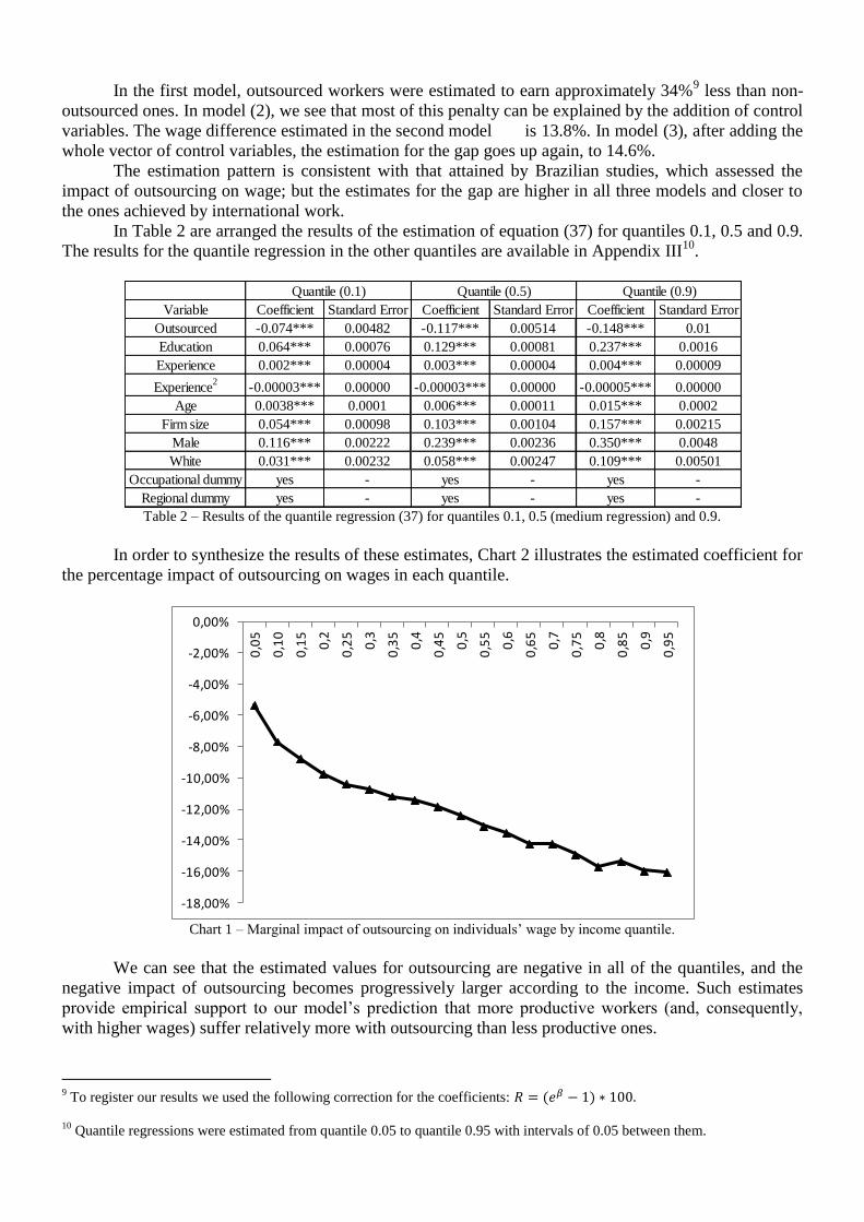
In the first model, outsourced workers were estimated to earn approximately 34%9 less than non-

outsourced ones. In model (2), we see that most of this penalty can be explained by the addition of control

variables. The wage difference estimated in the second model is 13.8%. In model (3), after adding the

whole vector of control variables, the estimation for the gap goes up again, to 14.6%.

The estimation pattern is consistent with that attained by Brazilian studies, which assessed the

impact of outsourcing on wage; but the estimates for the gap are higher in all three models and closer to

the ones achieved by international work.

In Table 2 are arranged the results of the estimation of equation (37) for quantiles 0.1, 0.5 and 0.9.

The results for the quantile regression in the other quantiles are available in Appendix III10

.

Table 2 – Results of the quantile regression (37) for quantiles 0.1, 0.5 (medium regression) and 0.9.

In order to synthesize the results of these estimates, Chart 2 illustrates the estimated coefficient for

the percentage impact of outsourcing on wages in each quantile.

Chart 1 – Marginal impact of outsourcing on individuals’ wage by income quantile.

We can see that the estimated values for outsourcing are negative in all of the quantiles, and the

negative impact of outsourcing becomes progressively larger according to the income. Such estimates

provide empirical support to our model’s prediction that more productive workers (and, consequently,

with higher wages) suffer relatively more with outsourcing than less productive ones.

9 To register our results we used the following correction for the coefficients: 𝑅 = (𝑒𝛽 − 1) ∗ 100.

10

Quantile regressions were estimated from quantile 0.05 to quantile 0.95 with intervals of 0.05 between them.


Outsourced -0.074*** 0.00482 -0.117*** 0.00514 -0.148*** 0.01

Education 0.064*** 0.00076 0.129*** 0.00081 0.237*** 0.0016

Experience 0.002*** 0.00004 0.003*** 0.00004 0.004*** 0.00009

Experience2

-0.00003*** 0.00000 -0.00003*** 0.00000 -0.00005*** 0.00000

Age 0.0038*** 0.0001 0.006*** 0.00011 0.015*** 0.0002

Firm size 0.054*** 0.00098 0.103*** 0.00104 0.157*** 0.00215

Male 0.116*** 0.00222 0.239*** 0.00236 0.350*** 0.0048

White 0.031*** 0.00232 0.058*** 0.00247 0.109*** 0.00501

Occupational dummy yes - yes - yes -

Regional dummy yes - yes - yes -

Quantile (0.1) Quantile (0.5) Quantile (0.9)

-18,00%

-16,00%

-14,00%

-12,00%

-10,00%

-8,00%

-6,00%

-4,00%

-2,00%

0,00%

0,0

5

0,1

0

0,1

5

0,2

0,2

5

0,3

0,3

5

0,4

0,4

5

0,5

0,5

5

0,6

0,6

5

0,7

0,7

5

0,8

0,8

5

0,9

0,9

5

5. Endogeneity bias

It is possible that there is some form of unobserved characteristics not orthogonal to the

occupational status that drove our previous results. This section tries to account for that.

5.1 New Database

In this section we use a confidential version of the RAIS database, described in subsection 4.2, for

the years of 2009 and 2010. Unlike the previous database, this version contains an individual unique

identifier for all workers, which allow us to follow each individual in time.

Instead of working with all individuals, we restrict the database in 2010 only to those individuals

who were outsourced (defined in the same way as described in section 4), obtaining approximately four

and a half million observations.

Then, we match those individuals with the database for the previous year. We have been able to

match a little less than four million individuals, approximately 86,7% of all outsourced workers in 201011

.

In this subsample, around one and a half million individuals were not outsourced in 2009.

Since all the workers in the new database were outsourced in 2010, we expect that all the

individuals in this subsample will have much similar characteristics and, therefore, the workers who were

outsourced in 2010 and were not in 2009 constitute a much better counter-factual than the one used in the

previous section. Next, we will re-estimate some of the previous equations with our new database.

5.2 Results

In table 3, we present the results for our estimates for equation (34), similar to those displayed in

table 1, for our new database:

Table 3 – Results of our GLS regression (34) using our new sample

We can see that the raw gap between outsourced workers is drastically smaller in model (1) of

table 3 than the estimated in table 1 – only -4,2%. Once we add additional control variables, the estimated

gap increases to approximately -7,9%, which is still smaller than the respective models in table 1. This

results points out that, in fact, unobserved characteristics seem to explain a large part of the outsourced

wage gap.

Next we re-estimate equation (37)12

for our database for quantiles 0.1, 0.5 and 0.9. The results are

presented in Table 4.

11

The non matched workers were not in the formal market in 2009. The rate of matched individuals achieved with this

procedure is very similar to the matching using all formal workers done by Belchior and Bertussi (2016). 12

Again, the estimation of the quantile regression was not computationally feasible even with the drastic reduction of the new

database size. Therefore, we applied the same method described in apendix II to obtain a new random subsample of our new

database.


Outsourced -0.041*** 0.0008 -0.074*** 0.0007 -0.076*** 0.0007

Education - - 0.181*** 0.00002 0.1754*** 0.0002

Experience - - 0.0041*** 0.00000 0.0044*** 0.00000

Experience2

- - -0.00004*** 0.00000 -0.00003*** 0.00000

Age - - -0.008*** 0.00000 0.0078*** 0.00001

Firm size - - - - 0.027*** 0.00008

Male - - - - 0.281*** 0.00019

White - - - - 0.091*** 0.00019

Occupational dummy no - no - yes -

Regional dummy no - no - yes -

Model (1) Model (2) Model (3)

Table 4 – Results of the quantile regression (37) for quantiles 0.1, 0.5 (medium regression) and 0.9 in our subsample.

First, we note that, when we control for selection bias, the wage gap is still negative and

statistically significant at the one percent level for the three quantiles. The magnitude of the wage gap,

however, is smaller than the previous in all three estimates – also indicating the importance of

unobservable effects. This effect seems to be relatively stronger for low productive workers as the

estimation for the (0.1) quantile got severely closer to zero and the estimation for the (0.9) quantile was

much closer to the original result.

In Chart 2, we present the estimates for the marginal impact of outsourcing on wages on each

quantile in order to summarize our results. Also, for comparative purposes, we plot the previous results

for the quantile regression displayed in Chart 2.

Chart 2 – Marginal impact of outsourcing on individuals’ wage by income quantile in the subsample (gray) and previous

quantile regression results as a baseline (black)

The graph confirms the previous conclusions drawn from Table 4. The entire distribution was

dragged up as we controlled for the unobservable characteristics. The effect, of course, is not the same for

different individuals. The coefficient for the poorest workers is slightly positive, despite not economically

or statistically significant, while for the richer individuals the coefficient is statistically indifferent for our

previous estimates. We argue that there must be unobservable individual characteristics, undesirable from

the viewpoint of the employer, that affect the occupational status of the workers. Although this

characteristics seem to be present in all distribution, they appear to be far more important for the less

productive individuals. The complete set of estimates for the quantile regression are displayed in

appendix III.


Outsourced -0.0150*** 0.0021 -0.0788*** 0.0025 -0.1208*** 0.0056

Education 0.0506*** 0.0006 0.1765*** 0.0007 0.2288*** 0.0017

Experience 0.0014** 0.00004 0.0044*** 0.00005 0.0066*** 0.0001

Experience2

-0.00003*** 0.00000 -0.00003*** 0.00000 -0.000009*** 0.00000

Age 0.0012*** 0.00009 0.0078*** 0.00011 0.0115*** 0.0002

Firm size 0.0043*** 0.0009 0.0288*** 0.0010 0.0514*** 0.0023

Male 0.0962*** 0.0019 0.2896*** 0.0022 0.3782*** 0.0050

White 0.0273*** 0.0017 0.0937*** 0.0021 0.1161*** 0.0046

Occupational dummy yes - yes - yes -

Regional dummy yes - yes - yes -

Quantile (0.1) Quantile (0.5) Quantile (0.9)

-18,00%

-16,00%

-14,00%

-12,00%

-10,00%

-8,00%

-6,00%

-4,00%

-2,00%

0,00%

2,00%

0,0

5

0,1

0

0,1

5

0,2

0,2

5

0,3

0,3

5

0,4

0,4

5

0,5

0,5

5

0,6

0,6

5

0,7

0,7

5

0,8

0,8

5

0,9

0,9

5

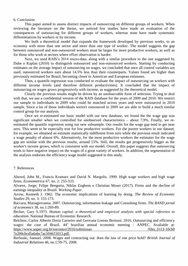
6. Conclusion

This paper aimed to assess distinct impacts of outsourcing on different groups of workers. When

reviewing the literature on the theme, we noticed few studies have made an evaluation of the

consequences of outsourcing for different groups of workers, whereas none have made systematic

differentiations by workers or by income.

We built a theoretical model that expands the framework developed by previous works, to an

economy with more than one sector and more than one type of worker. The model suggests the gap

between outsourced and non-outsourced workers must be larger for more productive workers, as well as

for those who work at sectors where effort observation is harder.

Next, we used RAIS’s 2014 micro-data, along with a similar procedure to the one suggested by

Dube e Kaplan (2010) to distinguish outsourced and non-outsourced workers. Starting by conducting

estimates on the average impact of outsourcing on wages, we concluded that once all control variables are

used, outsourced workers earn about 14.5% less than their counterparts. Values found are higher than

previously estimated for Brazil, becoming closer to American and European estimates.

Then, a quantile regression was conducted to evaluate the impact of outsourcing on workers with

different income levels (and therefore different productivities). It concluded that the impact of

outsourcing on wages grows progressively with income, as suggested by the theoretical model.

Clearly the previous results might be driven by an unobservable form of selection. Trying to deal

with that, we use a confidential version of the RAIS database for the years of 2009 and 2010. We restrict

our sample to individuals in 2009 who could be matched across years and were outsourced in 2010

sample. Since a lot of those individuals weren't outsourced in 2009 we are able to build a much similar

control group for our analysis.

Once we re-estimated our basic model with our new database, we found the the wage gap was

significant smaller when we controlled for unobserved characteristics – about 7,9%. Finally, we re-

estimated the quantile regression using our new subsample. Our results for the wage gap tend to get near

zero. This seem to be especially true for low productive workers. For the poorer workers in our dataset,

for example, we obtained an estimate statistically indifferent from zero while the previous result indicated

a wage penalty of almost 6%. Alternatively, for the most productive workers the estimates for the wage

gap are similar with the previous results, around 15%. Still, the results get progressively bigger as the

worker's income grows, which is consistent with our model. Overall, this paper suggests that outsourcing

tends to have negative impact on the wages of a great variety of workers. In addition, the segmentation of

the analysis endorses the efficiency wage model suggested in this study.

7. References

Abowd, John M., Francis Kramarz and David N. Margolis. 1999. High wage workers and high wage

firms. Econometrica 67, no. 2: 255-333.

Alvarez, Jorge; Felipe Benguria, Niklas Engbom e Christian Moser (2017). Firms and the decline of

earnings inequality in Brazil. Working Paper.

Arrow, Kenneth J. 1962. The economic implications of learning by doing. The Review of Economic

Studies 29, no. 3: 155-173.

Baccara, Mariagiovanna. 2007. Outsourcing, information leakage and Consulting firms. The RAND jornal

of economics 38, no.1:269-89.

Becker, Gary S.1975. Human capital: a theoretical and empirical analysis with special reference to

education. National Bureau of Economic Research.

Belchior, Carlos Alberto Doria Carneiro and Geovana Lorena Bertussi. 2016. Outsourcing and efficiency

wages: the case of Brazil. 44o

brazilian annual economic meeting - ANPEC. Avaliable at:

https://www.anpec.org.br/encontro/2016/submissao /files_I/i13-10cb0

7e200cbcd5a6abc7ac504615013.pdf.

Berlinski, Samuel. 2008. Wages and contracting out: does the law of one price hold? British Journal of

Industrial Relations 46, no.1:59-75, 2008.

Card, David, Jӧrg Heining and Patrick Kline. 2013. Workplace heterogeneity and the rise of West

German wage inequality. The Quarterly Journal of Economics 128, no.3:967-1015.

Dube, Arindrajit and Ethan Kaplan. 2010. Does outsourcing reduce the wages in low wages service

occupations? Evidence from janitors and guards. Industrial and Labour Relations Review 63, no.2: 287-

306.

Goldschmidt, Deborah e Johannes Schmieder. 2017. The rise of domestic outsourcing and the rise of

German wage structure. The Quarterly Journal of Economics, forthcoming.

Koenker, Roger, and Gilbert Basset Jr. 1978. Regression quantiles. Econometrica, 46, no.1: 33-50.

Koenker, Roger, and Kevin F. Hallock. 2001. Quantile regression. Journal of Economic Perspectives 15,

no.4: 143-156.

Krueger, Alan B., and Andreas I. Mueller. 2016. A contribution to the empirics of reservation wages.

American Economic Journal: Economic Policy, 8, no:1:142-79.

Mankiw, Gregory and Phillip Swagel. 2006. The politics and economics of offshore outsourcing. Journal

of monetary economics, 53, no.5, p.1027-56.

Oi, Walter Y., and Todd L. Idson. 1999. Firm size and wages. In Handbook of Labour Economics, ed.

David Card and Orley Ashenfelter. Elsevier.

Ramos, Carlos Alberto. 2012. Economia do Trabalho: modelos teóricos e o debate no Brasil. CRV,

Brasília.

SEBRAE. 2013. Anuário do trabalho na micro e pequena empresa. Avaliable at:

http://www.sebrae.com.br/Sebrae/Portal%20Sebrae/Anexos/Anuario%20do%20Trabalho%20Na%20Mic

ro%20e%20Pequena%20Empresa_2013.pdf.

Stein, Guilherme.; Eduardo Zylberstajn and Hélio Zylberstajn. Diferencial de salários da mão de obra

terceirizada no Brasil. São Paulo School of economics working paper, n.4, 2015.

Song, Jae, David J. Price, Fatih Guvenen, Nicholas Bloom and Till von Wachter. 2016. Firming up

inequality. National Bureau of Economic Research Working Paper, no.21199.

Williansom, Oilver. 2008. Outsourcing: transaction costs economics and supply chain management.

Journal of supply chain management, 44, no.2: 5-16.

7. Appendix I – Making of the database

The following table, developed by Belchior and Bertussi (2016), indicates the occupations

commonly considered as outsourced, as well as the sectors associated to them, implying the worker’s

occupational status.

CBO CNAE

CBO CNAE 513420 56201

1231 5135

1232 5136

1233

1234 CBO CNAE

1238 5141 81214

82113 5142

70204 5143

69117 5172

3511 82113 5173

252210 69206 81117

70204 81214

80111

CBO CNAE

1236 73114 CBO CNAE

1237 82113 9511

1425 631 7313

1426 620 7321

73203 7311

70204 7156

95118 7243

82202 7301

82113 8601

63119 9501

620 9502

631 9531

95118 9541

70204

620 CBO CNAE

631 7151

4223 7152

4222 7153

420135 7154

7155

CBO CNAE 7157

3141 43223 7161

28691 7162

3144 33147 7163

7164

33121 7165

33147 7166

61906 7170

43215 7201

7202

CBO CNAE 7211

5132 56201 7212

513425 81214 7241

513430 56201 7243

Professions

Professions

Professions

Profissões

Professions

71120

Security agent

5174Doorman

Eletricity Sector

Residencial sector

Elevator operator

Cleaner 81214

43991

Manual laborers and

builders

33210

Eletricity Sector

workers

Civil construction sector

80111

Cook

Server

61096

43215

951

952

63992

9151

9153

Mechanics and

maintenace specialists

Maintenance

technicians

3171Programmers

82202Telemarketing workers

Food Sector

IT and R&D

Professions

Directors of several

areas

Professions

Directors and workers

of R&D and IT

2123

Administrators and

network analysts

2410Lawyers

Professions

Food producer and

assistant56201

Barman

43215

Administrative Workers

82113

2124

Maintenance

Accountants

8. Appendix II – Creation of a Random Sub-sample

The random sub-sample was created using the pseudo-random number generator KISS, available

in the 13th

version of statistic software Stata. To carry out this procedure, first the seed s was established

in order to allow the replication of the randomization process. The seed used was 45002494 in the first

quantile regression and 98173938 for the second.

Next, we attributed a random value to each observation in the database, extracted from a uniform

distribution with extreme values 0 and 1:

𝑋~𝑈(0,1) Subsequently, the samples from the database were rearranged in ascending order according to the

value attributed to them, from the previous distribution. Finally, the random sub-sample was defined as

the first 250 thousand observations from the database after the rearrangement. The full sequence of

commands is:

set seed s

gen random=runiform()

sort random

gen insample=_n <= 250000

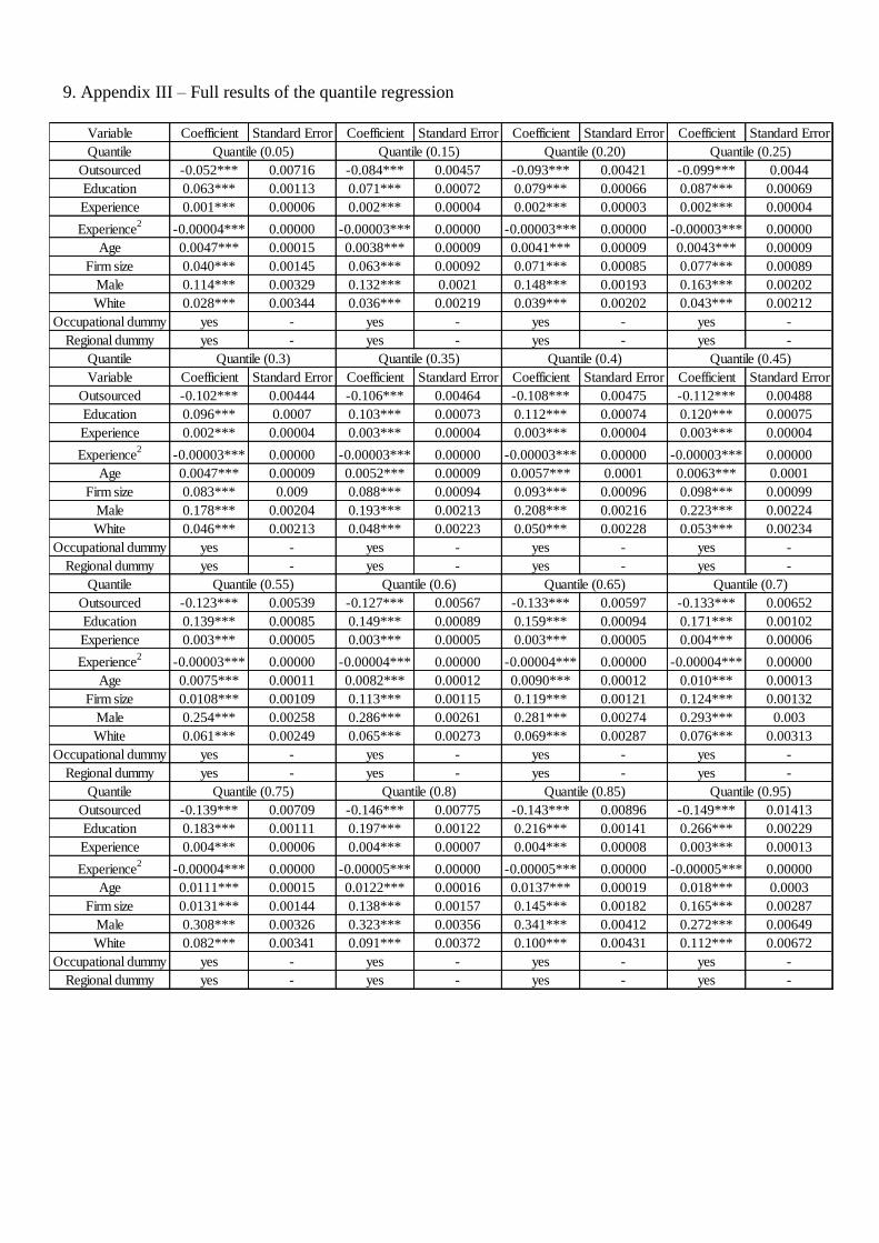
9. Appendix III – Full results of the quantile regression

Variable Coefficient Standard Error Coefficient Standard Error Coefficient Standard Error Coefficient Standard Error

Quantile

Outsourced -0.052*** 0.00716 -0.084*** 0.00457 -0.093*** 0.00421 -0.099*** 0.0044

Education 0.063*** 0.00113 0.071*** 0.00072 0.079*** 0.00066 0.087*** 0.00069

Experience 0.001*** 0.00006 0.002*** 0.00004 0.002*** 0.00003 0.002*** 0.00004

Experience2

-0.00004*** 0.00000 -0.00003*** 0.00000 -0.00003*** 0.00000 -0.00003*** 0.00000

Age 0.0047*** 0.00015 0.0038*** 0.00009 0.0041*** 0.00009 0.0043*** 0.00009

Firm size 0.040*** 0.00145 0.063*** 0.00092 0.071*** 0.00085 0.077*** 0.00089

Male 0.114*** 0.00329 0.132*** 0.0021 0.148*** 0.00193 0.163*** 0.00202

White 0.028*** 0.00344 0.036*** 0.00219 0.039*** 0.00202 0.043*** 0.00212

Occupational dummy yes - yes - yes - yes -

Regional dummy yes - yes - yes - yes -

Quantile


Outsourced -0.102*** 0.00444 -0.106*** 0.00464 -0.108*** 0.00475 -0.112*** 0.00488

Education 0.096*** 0.0007 0.103*** 0.00073 0.112*** 0.00074 0.120*** 0.00075

Experience 0.002*** 0.00004 0.003*** 0.00004 0.003*** 0.00004 0.003*** 0.00004

Experience2

-0.00003*** 0.00000 -0.00003*** 0.00000 -0.00003*** 0.00000 -0.00003*** 0.00000

Age 0.0047*** 0.00009 0.0052*** 0.00009 0.0057*** 0.0001 0.0063*** 0.0001

Firm size 0.083*** 0.009 0.088*** 0.00094 0.093*** 0.00096 0.098*** 0.00099

Male 0.178*** 0.00204 0.193*** 0.00213 0.208*** 0.00216 0.223*** 0.00224

White 0.046*** 0.00213 0.048*** 0.00223 0.050*** 0.00228 0.053*** 0.00234



Quantile

Outsourced -0.123*** 0.00539 -0.127*** 0.00567 -0.133*** 0.00597 -0.133*** 0.00652

Education 0.139*** 0.00085 0.149*** 0.00089 0.159*** 0.00094 0.171*** 0.00102

Experience 0.003*** 0.00005 0.003*** 0.00005 0.003*** 0.00005 0.004*** 0.00006

Experience2

-0.00003*** 0.00000 -0.00004*** 0.00000 -0.00004*** 0.00000 -0.00004*** 0.00000

Age 0.0075*** 0.00011 0.0082*** 0.00012 0.0090*** 0.00012 0.010*** 0.00013

Firm size 0.0108*** 0.00109 0.113*** 0.00115 0.119*** 0.00121 0.124*** 0.00132

Male 0.254*** 0.00258 0.286*** 0.00261 0.281*** 0.00274 0.293*** 0.003

White 0.061*** 0.00249 0.065*** 0.00273 0.069*** 0.00287 0.076*** 0.00313



Quantile

Outsourced -0.139*** 0.00709 -0.146*** 0.00775 -0.143*** 0.00896 -0.149*** 0.01413

Education 0.183*** 0.00111 0.197*** 0.00122 0.216*** 0.00141 0.266*** 0.00229

Experience 0.004*** 0.00006 0.004*** 0.00007 0.004*** 0.00008 0.003*** 0.00013

Experience2

-0.00004*** 0.00000 -0.00005*** 0.00000 -0.00005*** 0.00000 -0.00005*** 0.00000

Age 0.0111*** 0.00015 0.0122*** 0.00016 0.0137*** 0.00019 0.018*** 0.0003

Firm size 0.0131*** 0.00144 0.138*** 0.00157 0.145*** 0.00182 0.165*** 0.00287

Male 0.308*** 0.00326 0.323*** 0.00356 0.341*** 0.00412 0.272*** 0.00649

White 0.082*** 0.00341 0.091*** 0.00372 0.100*** 0.00431 0.112*** 0.00672



Quantile (0.05) Quantile (0.15) Quantile (0.20) Quantile (0.25)





Quantile

Outsourced 0.0064 0.0042 -0.0287*** 0.0020 -0.0395*** 0.0020 -0.0482*** 0.0020

Education 0.0606*** 0.0013 0.0567*** 0.0006 0.0667*** 0.00063 0.0754*** 0.00064

Experience 0.0017*** 0.00009 0.0016*** 0.00004 0.0019*** 0.00004 0.0021*** 0.00004

Experience2

-0.00002*** 0.00000 -0.00001*** 0.00000 -0.00001*** 0.00000 -0.00001*** 0.00000

Age 0.0018*** 0.0001 0.0011*** 0.00008 0.0013*** 0.00008 0.0017*** 0.00008

Firm size 0.000005 0.0017 0.0068*** 0.00085 0.0089*** 0.00085 0.077*** 0.00089

Male 0.1325*** 0.0037 0.1033*** 0.0018 0.1205*** 0.0018 0.163*** 0.00202

White 0.0291*** 0.0035 0.0339*** 0.0016 0.0406*** 0.0016 0.043*** 0.00212



Quantile


Outsourced -0.0557*** 0.0022 -0.0614*** 0.0021 -0.066*** 0.0022 -0.0714*** 0.0024

Education 0.0831*** 0.00068 0.0900*** 0.00066 0.0973*** 0.00071 0.1053*** 0.00075

Experience 0.0022*** 0.00004 0.0023*** 0.00004 0.0024*** 0.00004 0.0026*** 0.00005

Experience2

-0.00001*** 0.00000 -0.00004 0.0002 -0.00004* 0.00002 -0.00001*** 0.00000

Age 0.0020*** 0.00009 0.0022*** 0.00008 0.0026*** 0.00009 0.0031*** 0.0001

Firm size 0.0120*** 0.009 0.0142*** 0.00089 0.0148*** 0.00096 0.0162*** 0.0010

Male 0.157*** 0.0019 0.1742*** 0.0019 0.1916*** 0.0020 0.2083*** 0.0021

White 0.0499*** 0.0018 0.0542*** 0.0017 0.0566*** 0.0018 0.0612*** 0.0020



Quantile

Outsourced -0.772*** 0.0027 -0.0798*** 0.0029 -0.0825*** 0.0032 -0.0857*** 0.0036

Education 0.1237*** 0.00087 0.1334*** 0.0009 0.144*** 0.0010 0.1564*** 0.0011

Experience 0.003*** 0.00006 0.0033*** 0.00005 0.0037*** 0.00007 0.0042*** 0.00008

Experience2

-0.00002*** 0.00000 -0.00001*** 0.00000 -0.00009*** 0.00003 -0.00005 0.00003

Age 0.0042*** 0.00011 0.0048*** 0.00012 0.0055*** 0.0001 0.0063*** 0.00015

Firm size 0.0198*** 0.0011 0.0215*** 0.0012 0.0249*** 0.0013 0.0288*** 0.0015

Male 0.2437*** 0.0024 0.2631*** 0.0026 0.2827*** 0.0029 0.3022*** 0.0032

White 0.0688*** 0.0023 0.0741*** 0.0024 0.0799*** 0.0027 0.0848*** 0.0029



Quantile

Outsourced -0.0909*** 0.0039 -0.0963*** 0.0043 -0.1066*** 0.0049 -0.1453*** 0.0076

Education 0.1710*** 0.0012 0.1861*** 0.0013 0.2046*** 0.0015 0.2641*** 0.0023

Experience 0.0047*** 0.00008 0.0054*** 0.00009 0.006*** 0.0001 0.0069*** 0.00017

Experience2

-0.00002*** 0.00000 -0.00004*** 0.00000 -0.00007*** 0.00000 -0.00001*** 0.00000

Age 0.0074*** 0.00015 0.0083*** 0.00018 0.0098*** 0.0002 0.0145*** 0.0003

Firm size 0.0334*** 0.0016 0.0385*** 0.0018 0.0447*** 0.0020 0.0572*** 0.0032

Male 0.3241*** 0.0035 0.3444*** 0.0038 0.3616*** 0.0044 0.4036*** 0.0068

White 0.0910*** 0.0032 0.0984*** 0.0036 0.1069*** 0.0040 0.1215*** 0.0063







heterogeneous impacts of domestic outsourcing on wages ... · heterogeneous impacts of domestic...

Documents