hex-splines: a novel spline family for hexagonal latticesbig · a novel spline family for hexagonal...

ACCEPTED FOR PUBLICATION IN IEEE TRANSACTIONS ON IMAGE PROCESSING 1

Hex-splines:

A novel spline family for hexagonal lattices

Dimitri Van De Ville, Thierry Blu, Michael Unser,

Wilfried Philips, Ignace Lemahieu, Rik Van de Walle

D. Van De Ville, T. Blu, M. Unser are with the Biomedical Imaging Group (BIG), Swiss Federal Institute of Technology

Lausanne (EPFL), Switzerland. I. Lemahieu, R. Van de Walle are with ELIS, Ghent University, Ghent, Belgium. W. Philips

is with TELIN, Ghent University, Ghent, Belgium.

October 29, 2003 DRAFT


Abstract

This paper proposes a new family of bivariate, non-separable splines, called hex-splines, especially designed for hexagonal

lattices. The starting point of the construction is the indicator function of the Voronoi cell, which is used to define in a

natural way the first-order hex-spline. Higher order hex-splines are obtained by successive convolutions. A mathematical

analysis of this new bivariate spline family is presented. In particular, we derive a closed form for a hex-spline of arbitrary

order. We also discuss important properties, such as their Fourier transform and the fact they form a Riesz basis. We

also highlight the approximation order. For conventional rectangular lattices, hex-splines revert to classical separable tensor-

product B-splines. Finally, some prototypical applications and experimental results demonstrate the usefulness of hex-splines

for handling hexagonally sampled data.

Keywords

Bivariate splines, hexagonal lattices, approximation theory, sampling theory

I. Introduction

Digital image processing systems require a sampling strategy to represent two-dimensional data. The

common approach is to take the samples on a rectangular lattice. Another possibility is to use hexagonal

sampling, which provides several advantages [1, 2]. For instance, a hexagon has a twelve-fold symmetry

as compared to the eight-fold of a square. Due to the improved packing density, hexagonal lattices are

better suited for representing isotropically bandlimited signals. The higher degree of symmetry can also

be used to design more isotropic filters to be applied on hexagonal lattices [2–4]. The six neighbors of a

hexagonal cell and their connectivity is well-defined [5] and has been used for better edge detection [6, 7]

and pattern recognition [8–11].

An important issue in image processing is the link between the discrete and the continuous domain. A

discrete/continuous model is essential for computational tasks such as interpolation and resampling. B-

spline models are especially popular and have been succesfully applied to image processing on rectangular

lattices using tensor-product basis functions. This paper introduces a novel spline family, the so-called

hex-splines, which provide a discrete/continuous model suitable for hexagonally sampled data. These

new bivariate splines take into account the shape of the Voronoi cell and build up higher order splines

by successive convolutions. For rectangular lattices, these splines revert to the classical tensor-product

B-splines. The hex-splines were first introduced in our paper [12] from an application point of view

(without an analytical expression). This paper presents a mathematical analysis of the hex-splines which

contributes to a better understanding of their properties. Additionally, we discuss the algorithms that are

needed to use these splines in practice.

The presentation is organized as follows. In Sect. II, we review the fundamental properties of lattices,

cells, and one-dimensional B-splines. Next, we introduce and derive the hex-splines and discrete hex-

splines. In Sect. V, we present some basic applications of the hex-splines to image processing.

There are some notational conventions we apply throughout this paper. Vectors are denoted in bold

and lowercase, e.g., x = [x1 x2]T, while a matrix is bold and uppercase, e.g., A. The Fourier transform



of a function f(x) is defined as f(ωωω) =∫

f(x) exp(−j〈ωωω,x〉)dx. The complex conjugate is indicated by

f(x)?. The inner product of two functions f1 and f2 is denoted as 〈f1, f2〉 and the convolution as f1 ∗ f2.

II. Splines for hexagonal lattices

A. Lattices

Two-dimensional periodic lattices are characterized by two (linearly independant) vectors r1 and r2.

Any integer combination rk = k1r1 + k2r2 of these vectors points to a lattice site. It is often convenient

to group the lattice vectors r1 and r2 in a matrix

R = [r1 r2] , (1)

such that the lattice sites are given by Rk, where k = [k1 k2]T.

A well-defined and unique tiling cell is the Voronoi cell, which contains all points that are closer to their

lattice site than to any other site. The indicator function for the Voronoi cell of the origin is defined as:

χR(x) =

1, x ∈ Voronoi cell,

1/mx, x ∈ edge of the Voronoi cell,

0, x /∈ Voronoi cell,

(2)

where mx is the number of lattice points to which x is adjacent. Note that χR(x) tiles the plane by

definition.

The dual or reciprocal lattice is specified by R = [r1 r2] =(R−1

)T= R−T. The reciprocal lattice

vectors therefore satisfy the relation 〈rk, rl〉 = δk−l, where δk is the kronecker-delta sequence. We mention

two useful relationships where the dual lattice becomes important. Assume we have a function f(x) and

its Fourier transform f(ωωω). Let fM(x) = f(Mx). Then it is well known that

fM(ωωω) = f(M−Tωωω)/ |detM| . (3)

Likewise, the Poisson sum formula on a lattice R is (see App. A for the proof)

∑

k

f(x−Rk) =1

|det(R)|∑

k

f(2πRk) exp(j2π⟨RTk,x

⟩). (4)

The case of special interest in this article is the regular hexagonal lattice of the second type, which is

characterized by matrices

R =

√3

2 0

− 12 1

, R =

2√

33

√3

3

0 1

. (5)

Figure 1 shows the lattice vectors and the Voronoi cell of R and R. The reciprocal Voronoi cell can be

considered as the “natural Nyquist region”; in other words, the effect of sampling a signal on a lattice R

is to replicate its spectrum on the lattice sites 2πRk. For more details about lattices and cells, we refer

to [13, 14].



(a) (b)

r1

r2

r1

r2

Fig. 1. (a) The regular hexagonal lattice of the second type and its Voronoi cell. (b) The dual lattice.

B. Sinc-function for hexagonal lattices

In this section, we extend the sampling theorem for hexagonal lattices. For a given lattice characterized

by a matrix R, we define the sincH-function of the corresponding reciprocal lattice R as the Fourier

transform of the indicator function of the Voronoi cell:

χR(ωωω) = Ω sincHR

(ωωω/(2π)), (6)

where we introduce the normalization by the surface area of the Voronoi cell Ω , |det(R)|. By definition,

the function χR(x) tiles the plane when replicated on the lattice sites of R. So we have

∑

k

χR(x−Rk) = 1, ∀x. (7)

When we plug in this condition into the Poisson sum formula of Eq. (4), which holds for all x, we obtain

sincHR

(Rk) = δk, (8)

where we have used χR(ωωω) as defined in Eq. (6). This function takes the value 1 at the origin and 0 at

the reciprocal lattice sites, as we expect from a properly defined sinc-function. By duality, it follows that

the sincH-function corresponding to the lattice matrix R satisfies the interpolation property in the spatial

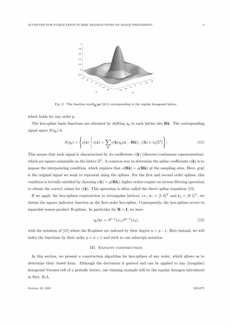
domain. An explicit formula for the sincH-function is derived in Sect. IV-A. This function is shown in

Fig. 2.

C. Hex-splines

We define the first-order hex-spline as η1(x) = χR(x). Hex-splines of higher orders are constructed by

successive convolutions:

ηp+1(x) =η1 ∗ ηp(x)

Ω, p ≥ 1. (9)

Some examples of hex-splines are shown in Fig. 3. An important property, which is satisfied automatically

due to Eq. (7) and the construction rule of Eq. (9), is the partition of unity:

∑

k

ηp(x−Rk) = 1, ∀x, (10)



−15−10

−50

510

15

−15−10

−50

510

15

−0.2

0

0.2

0.4

0.6

0.8

1

ω1

ω2

Fig. 2. The function sincHR

(ωωω/(2π)) corresponding to the regular hexagonal lattice.

which holds for any order p.

The hex-spline basis functions are obtained by shifting ηp to each lattice site Rk. The corresponding

signal space S(ηp) is

S(ηp) =

s(x)

∣∣∣∣∣ s(x) =∑

k

c(k)ηp(x−Rk); c(k) ∈ l2(Z2)

. (11)

This means that each signal is characterized by its coefficients c(k) (discrete/continuous representation),

which are square-summable on the lattice Z2. A common way to determine the spline coefficients c(k) is to

impose the interpolating condition, which requires that s(Rk) = g(Rk) at the sampling sites. Here, g(x)

is the original signal we want to represent using the splines. For the first and second order splines, this

condition is trivially satisfied by choosing c(k) = g(Rk); higher orders require an inverse filtering operation

to obtain the correct values for c(k). This operation is often called the direct spline transform [15].

If we apply the hex-splines construction to rectangular lattices, i.e., r1 = [1 0]T and r2 = [0 1]T, we

obtain the square indicator function as the first-order hex-spline. Consequently, the hex-splines revert to

separable tensor-product B-splines. In particular for R = I, we have

ηp(x) = βp−1(x1)βp−1(x2), (12)

with the notation of [15] where the B-splines are indexed by their degree n = p− 1. Here instead, we will

index the functions by their order p = n + 1 and stick to our subscript notation.

III. Explicit construction

In this section, we present a construction algorithm for hex-splines of any order, which allows us to

determine their closed form. Although the derivation is general and can be applied to any (irregular)

hexagonal Voronoi cell of a periodic lattice, our running example will be the regular hexagon introduced

in Sect. II-A.



(a) (b)

−2−1.5

−1−0.5

00.5

11.5

2

−2

−1

0

1

20

0.2

0.4

0.6

0.8

1

x1x2 −2

−1.5−1

−0.50

0.51

1.52

−2

−1.5

−1

−0.5

0

0.5

1

1.5

20

0.2

0.4

0.6

0.8

1

x1x2

(c) (d)

−2−1.5

−1−0.5

00.5

11.5

2

−2

−1.5

−1

−0.5

0

0.5

1

1.5

20

0.2

0.4

0.6

0.8

1

x1x2 −2

−1.5−1

−0.50

0.51

1.52

−2

−1.5

−1

−0.5

0

0.5

1

1.5

20

0.2

0.4

0.6

0.8

1

x1x2

Fig. 3. Hex-splines. (a) First order (p = 1). (b) Second order (p = 2). (c) Third order (p = 3). (d) Fourth order (p = 4).

A. B-spline refresher

Our construction is inspired by the properties of one-dimensional B-splines. It is well-known that B-

splines can be generated by using a suitable linear combination of shifted one-sided power functions. For

instance, the first-order B-spline can be expressed as

β0(x) = ∆ ∗ (x)0+ (13)

= (x + 1/2)0+ − (x − 1/2)0+, (14)

where ∆ denotes the central finite difference filter δ(x + 1/2) − δ(x − 1/2) and where (x)0+ is the unit

step function. The application of the finite difference to the step function, which is infinitely supported,

produces a compactly supported function. Figure 4 graphically illustrates the generation of β0. We

now examine the convolutional properties of the components ∆ and (x)0+. The n-fold convolution of the

localization operator results into the n-th order finite difference

∆ ∗∆n−1 = ∆n ←→ (exp(jω/2)− exp(−jω/2))n, (15)



(a)

β0(x)

1/2−1/2

x

1

(b)

(x)0+

x

1/2−1/2

1

1

Fig. 4. (a) The one-dimensional first-order B-spline β0(x). (b) Construction of β0(x) by the step function (x)0+ and the

finite difference ∆.

which is conveniently specified by its Fourier expression. Analogously, successive convolutions of the step

function yield the one-sided power functions:

(x)0+0!∗ (x)n−1

+

(n− 1)!=

(x)n+

n!=

max(0, x)n

n!, (16)

which are the generating functions of higher order splines.

Relations (15) and (16) are especially useful for deriving the following explicit formula, starting from

the convolutional definition of B-splines:

βn = β0 ∗ . . . ∗ β0

︸︷︷︸n+1 times

=(∆ ∗ (x)0+

)∗ . . . ∗

(∆ ∗ (x)0+

)

= ∆n+1 ∗ (x)n+

n!.

The corresponding two-dimensional B-splines on a rectangular lattice are obtained by simple application

of the tensor-product: βn(x) = βn(x1)βn(x2). Due to the separability, the generating function becomes

(x)n+ = (x1)

n+(x2)

n+ and the localization operator ∆x1

∗∆x2. So for n = 0, a generating function (which

fills the upper right quadrant of the plane) is placed on each corner of a square with an appropriate weight.

B. Construction of the first-order hex-spline

Now, we aim at a similar construction for hex-splines. Let us start by putting together the first-order

hex-spline η1 in a graphical way. We want the generating function to resemble (x)0+ but we also need



(x)0+

(x)0/

(x)0\

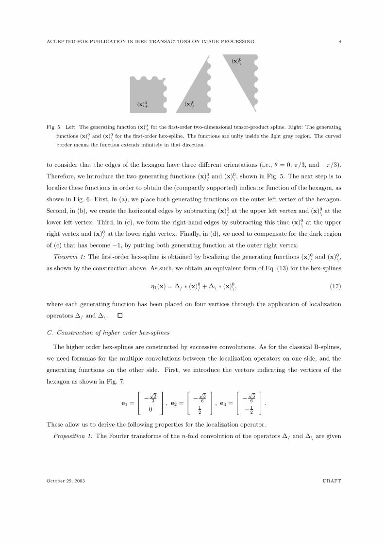
Fig. 5. Left: The generating function (x)0+ for the first-order two-dimensional tensor-product spline. Right: The generating

functions (x)0/

and (x)0\

for the first-order hex-spline. The functions are unity inside the light gray region. The curved

border means the function extends infinitely in that direction.

to consider that the edges of the hexagon have three different orientations (i.e., θ = 0, π/3, and −π/3).

Therefore, we introduce the two generating functions (x)0/ and (x)0\, shown in Fig. 5. The next step is to

localize these functions in order to obtain the (compactly supported) indicator function of the hexagon, as

shown in Fig. 6. First, in (a), we place both generating functions on the outer left vertex of the hexagon.

Second, in (b), we create the horizontal edges by subtracting (x)0/ at the upper left vertex and (x)0\ at the

lower left vertex. Third, in (c), we form the right-hand edges by subtracting this time (x)0\ at the upper

right vertex and (x)0/ at the lower right vertex. Finally, in (d), we need to compensate for the dark region

of (c) that has become −1, by putting both generating function at the outer right vertex.

Theorem 1: The first-order hex-spline is obtained by localizing the generating functions (x)0/ and (x)0\,

as shown by the construction above. As such, we obtain an equivalent form of Eq. (13) for the hex-splines

η1(x) = ∆/ ∗ (x)0/ + ∆\ ∗ (x)0\, (17)

where each generating function has been placed on four vertices through the application of localization

operators ∆/ and ∆\.

C. Construction of higher order hex-splines

The higher order hex-splines are constructed by successive convolutions. As for the classical B-splines,

we need formulas for the multiple convolutions between the localization operators on one side, and the

generating functions on the other side. First, we introduce the vectors indicating the vertices of the

hexagon as shown in Fig. 7:

e1 =

−

√3

3

0

, e2 =

−

√3

6

12

, e3 =

−

√3

6

− 12

.

These allow us to derive the following properties for the localization operator.

Proposition 1: The Fourier transforms of the n-fold convolution of the operators ∆/ and ∆\ are given



(a) (b)

+1/+1\

−1/

−1\

(c) (d)

−1/

−1\

+1/

+1\

Fig. 6. The construction of the first-order hex-spline step-by-step. The light gray and dark gray regions correspond

respectively to +1 and −1.

e1

e2

e3

−e1

−e2

−e3

+1/+1/

+1\+1\

−1/

−1/ −1\

−1\

Fig. 7. The vectors e1, e2, and e3 are introduced to indicate the vertices of the hexagon. In order to build up the first-order

hex-spline, the two generating functions need to be placed at four vertices each, with the weights indicated.

by

∆n/ ←→

(∆(〈e1 + e2,ωωω〉)∆(〈e1 − e2,ωωω〉)

)n

∆n\ ←→

(∆(〈e1 + e3,ωωω〉)∆(〈e1 − e3,ωωω〉)

)n

where ∆(ω) = exp(jω/2) − exp(−jω/2) is the classical one-dimensional B-spline localization operator.



For the generating functions, we first introduce a way to describe them more precisely. For instance,

consider the generating function (x)0/. If the vectors u1 and u2 are along the border of the support, we

can define this function as

(x)0/ =

1, when 〈u1,x〉 > 0 and 〈u2,x〉 > 0

0, otherwise.(18)

The vectors u1 and u2 are the reciprocal ones of u1 and u2 (i.e., 〈uk, ul〉 = δk,l), see Fig. 8. Now, a more

general generating function is proposed which builds up higher polynomial degrees along the reciprocal

directions:

(x)(n1,n2)(u1,u2)

=(〈u1,x〉)n1

+

n1!

(〈u2,x〉)n2

+

n2!(19)

We also use the shorthand notation (x)n(u1,u2)

for (x)(n,n)(u1,u2)

. Note that this generating function can be

derived from the orthogonal case by the coordinate transformation given by the matrix M = [u1 u2]T.

For convenience, we have included the normalization by n1!n2! inside the definition of the generating

function. Next we choose u1 = [1 0]T and u2 such that |det(M)| = 1; i.e., the vertical component of u2

needs to be ±1 due to initial choice of u1. That way, we can describe (x)0/ and (x)0\ as

(x)0/ = (x)0(u1,u2),

(x)0\ = (x)0(u1,u3),

where

u1 =

1

0

, u2 =

√3

3

1

, u3 =

√3

3

−1

.

These vectors may also be expressed in terms of e1, e2, and e3:

u1 = − e1

‖e1‖, u2 =

e2 − e1⟨e2 − e1, [0 1]

T⟩ , u3 =

e3 − e1⟨e3 − e1, [0 − 1]

T⟩ . (20)

Next, we give the convolution rules for these generating functions (cf. proof in Appendix B).

Proposition 2: The generating functions, as defined before, satisfy the following recurrence equation:

(x)0(u1,u2)∗ (x)n−1

(u1,u2)= (x)n

(u1,u2). (21)

Crossterms, such as

(x)n1

(u1,u2)∗ (x)n2

(u1,u3), (22)

are denoted as (x)(n1+n2+1,n1,n2)(u1,u2,u3)

. Although this notation has no direct (spatial) interpretation in the

sense of Eq. (19), it can be studied in the Fourier domain as we will show in Sect. IV-A. For now, we only

mention how they can be computed in a recursive way:

(x)(n1,n2,n3)(u1,u2,u3)

=1

2〈u1,u2〉((x)

(n1+1,n2−1,n3)(u1,u2,u3)

+ (x)(n1+1,n2,n3−1)(u1,u2,u3)

), n1, n2, n3 ≥ 0. (23)



u1 = [1 0]T

u2u2

u1

Fig. 8. The two-dimensional generating function. The vectors u1 and u2 make up the borders of the support. The

polynomial degree increases along the reciprocal vectors u1 and u2 for higher order generating functions.

This can be applied recursively until the second or third power of a generating function equals −1, in

particular (x)(n1,−1,n3)(u1,u2,u3)

= (x)(n1,n3)(u1,u3)

and (x)(n1,n2,−1)(u1,u2,u3)

= (x)(n1,n2)(u1,u2)

.

Notice that the generating functions (x)(n1,n2)(u1,u2)

and (x)(n1,n2)(u1,u3)

are homogeneous two-dimensional polyno-

mials of degree n1 + n2; i.e., they satisfy the equation f(λx) = λn1+n2f(x). Consequently, the crossterms

are homogeneous polynomials as well. For example,

(x)0(u1,u2)∗ (x)0(u1,u3)

= (x)(1,0,0)(u1,u2,u3)

=

√3

2

((x)

(2,0)(u1,u3)

+ (x)(2,0)(u1,u2)

)(24)

is a homogeneous polynomial of degree 2.

Theorem 2: The higher-order hex-spline is obtained by applying the construction rule of Eq. (9) to

Eq. (17):

ηp(x) =1

Ωp−1

p∑

k=0

(p

k

)∆k

/ ∗∆p−k\ ∗ (x)k−1

(u1,u2)∗ (x)p−1−k

(u1,u3)

=1

Ωp−1

p∑

k=0

(p

k

)∆k

/ ∗∆p−k\ ∗ (x)

(p−1,k−1,p−1−k)(u1,u2,u3)

,

for p ≥ 1, where generating functions to the power −1 “neutralize” the convolution, i.e., (x)−1(u1,u2)

=

(x)−1(u1,u3)

= δ(x).

To facilitate the computation of these formulas for any order p, we have made available on the web an

implementation for the Maple mathematical software package (see Appendix D).

IV. Hex-spline properties

A. Fourier transform

From distribution theory, we know the Fourier transform of the one-sided power function:

(x)n+

n!←→ 1

(jω)n+1+

πjnδ(n)(ω)

n!, (25)

where δ(n) is the n-th derivative of the Dirac δ-function. There is also a “two-sided” generating function:

(x)nsign

n!=

xnsign(x)

2 n!=

(x)n+ + (−1)n+1(−x)n

+

2 n!←→ 1

(jω)n+1. (26)



Both generating functions are equivalent with respect to the localization operators (finite difference), i.e.,

the localization operator cancels the polynomial represented by the Dirac of the one-sided function, so

leaving the two-sided version. This mechanism is well-known in 1D and it is often used to allow simpler

Fourier domain manipulations.

For the two-dimensional extension by the tensor-product we obtain

(x1)n1

sign

n1!

(x2)n2

sign

n2!←→ 1

(jω1)n1+1(jω2)n2+1. (27)

The sign-version of (x)(n1,n2)(u1,u2)

can be defined by considering

|x|(n1,n2)(u1,u2)

=(〈x, u1〉)n1

sign

n1!

(〈x, u2〉)n2

sign

n2!, (28)

which corresponds to a coordinate transformation of the left-hand side of Eq. (27) by the matrix

M = [u1 u2]T

= [u1 u2]−1

(29)

Therefore, the Fourier transform of such a generating function is given by

|x|(n1,n2)(u1,u2)

←→ 1

(j〈u1,ωωω〉)n1+1(j〈u2,ωωω〉)n2+1, (30)

since |det(M)| = 1 due to the proper choice of u1 and u2. We refer to appendix C for a precise explanation

of how the sign-version of the generating function gets localized in two dimensions.

The localization process is a convolution which corresponds to a product in the Fourier domain. Putting

the pieces together, we get the Fourier transform of the first-order regular hex-spline

η1(ωωω) = ∆/ (x)0/ + ∆\ (x)0\

=2√

3

ω1

(cos(−ω1/(2

√3) + ω2/2)− cos(ω1/

√3)

ω1 +√

3ω2

+

cos(ω1/(2√

3) + ω2/2)− cos(ω1/√

3)

ω1 −√

3ω2

)(31)

= Ω sincHR

(ωωω/(2π)),

where we have used

∆/ = 2 cos(〈e1,ωωω〉)− 2 cos(〈e2,ωωω〉) = 2 cos(ω1/√

3)− 2 cos(−ω1/(2√

3) + ω2/2),

(x)0/ = − 1

〈u1,ωωω〉〈u2,ωωω〉= − 1

ω1(ω1/√

3 + ω2).

Equation (31) also provides us with an explicit expression for the sincH-function introduced in Sect. II-B.

Due to the simple recipe of Eq. (9), the Fourier transform for a hex-spline of order p can be derived

from η1(ωωω) as

ηp(ωωω) =(η1(ωωω))

p

Ωp−1= Ω sincH

R(ωωω/(2π))p. (32)



B. Riesz basis property

An important condition for the hex-splines to provide a sensible continuous/discrete model is to be stable

(i.e., a small variation of the coefficients results into a small variation of the function) and unambiguous

(i.e., each set of coefficients represents a unique function). Therefore, the basis functions should form a

Riesz basis, which requires the existence of two strictly positive constants 0 < A0 and A1 < +∞ such

that

A0 ||c||2 ≤∣∣∣∣∣

∣∣∣∣∣∑

k

c(k)ηp(x −Rk)

∣∣∣∣∣

∣∣∣∣∣

2

≤ A1 ||c||2 , (33)

using the Euclidean norm. This expression is equivalent to

ΩA0 ≤∑

k

∣∣∣ηp(ωωω + 2πRk)∣∣∣2

≤ ΩA1, (34)

where the central term is the Fourier transform of the sampled autocorrelation function

aηp(k) = 〈ηp(x −Rk), ηp(x)〉 = Ω η2p(Rk), (35)

and can be rewritten as aηp(ωωω) =

∑k

aηp(k) exp(−j〈ωωω,Rk〉).

Next, we explicitly demonstrate that such constants A0, A1 can be found for the case of a regular

hexagon. The upper bound is obtained from

aηp(ωωω) =

∑

k

ηp ∗ ηp(Rk) exp(−j〈ωωω,Rk〉)

≤∑

k

|ηp ∗ ηp(Rk)|

≤ Ω∑

k

|η2p(Rk)|

≤ Ω∑

k

η2p(Rk) = Ω =

√3

2= ΩA1,

where we have used the positivity of the hex-splines, the partition of unity of Eq. (10) and Eq. (9).

The derivation of the lower bound is slightly more involved. First, since aηp(ωωω) is periodic on 2πR,

we can concentrate our attention on the reciprocal tiling cell (i.e., the Nyquist region, characterized by



χ2πR

(ωωω) = 1). As such, we obtain

aηp(ωωω) =

∑

k

∣∣∣ηp(ωωω + 2πRk)∣∣∣2

=∑

k

∣∣∣η1(ωωω + 2πRk)∣∣∣2p

/Ω2(p−1)

≥ |η1(ωωω)|2p/Ω2(p−1)

= Ω2∣∣sincH

R(ωωω/(2π))

∣∣2p

≥ Ω2

∣∣∣∣ infχ2πR

(ωωω)=1sincH

R(ωωω/(2π))

∣∣∣∣2p

=3

4

(9 + 2

√3π

4π2

)2p

= ΩA0.

Indeed, the sincH-function decreases monotonically from the origin to the border of the Nyquist region

(see also Fig. 2). At the outer vertices it reaches its minimum, e.g., at ωωω = [0 4π/3]T, which yields A0.

C. Relation to other spline families

To the best knowledge of the authors, the hex-splines have not been proposed before. Nevertheless,

there is a connection with bivariate box-splines [16].

Two-dimensional box-splines are a family of bivariate splines. They are composed out of basic elements

that can be regarded as a causal B-spline along a vector; i.e., in Fourier, a basic element along a vector u

can be expressed as

M[u](ωωω) =1− exp(j〈ωωω,u〉)

j〈ωωω,u〉 . (36)

In the spatial domain, such an element corresponds to

M[u](x) = δ(〈u⊥,x〉)β0 (〈u,x〉 − 1/2) ,

for normalized u and u⊥ perpendicular to u. For example, for u = [1 0]T we obtain δ(x2)β0(x1− 1/2). A

general box-spline can be obtained by performing convolutions of these basic elements (so multiplications

of Eq. (36) in the Fourier domain). For instance, the box-spline M[e1 e2] (where e1 and e2 are linearly

independant) corresponds to the indicator function of the rhomboid spanned by e1 and e2, scaled by the

reciprocal of its surface area. Adding any direction by introducing a third vector, creates a “slope” (i.e.,

linearly increasing/decreasing) in that particular direction. It is therefore not possible to construct the

first-order hex-spline in this way. Nevertheless, the hex-spline can be constructed as the sum of three

box-splines using vectors along the borders of the hexagon:

η1(x) = |det [v1 v2]|M[v1 v2](x) + |det [v2 v3]|M[v2 v3](x) + |det [v1 v3]|M[v1 e3](x), (37)

where v1 = −e3 − e2, v2 = −e3 + e1, v3 = −e2 + e1. Figure 9 shows how the box-splines, each one

corresponding to the indicator function of a gray rhomboid, sum up to the regular hexagon, a case where

v1 = −e1, v2 = e2, and v3 = e3.



e2

e3

−e1

Fig. 9. Construction of the regular first-order hex-spline by the sum of three box-splines.

Fig. 10. Triangular mesh for the second-order hex-spline. There is one polynomial expression inside each triangle. Due to

the twelve-fold symmetry, the computation can be restricted to three triangles.

For the regular case, the box-spline equivalence automatically implies that the function is a polynomial

within each triangle inside the triangular mesh spanned by e1, e2, and e3 [17]. This property tells us that

we only need to determine the analytical form of the hex-splines in a limited number of regions. Figure 10

shows the triangular mesh for the second-order hex-spline, which separates the piecewise polynomial

regions.

Sablonniere et al. [18] introduced other families of splines, one of them with a hexagonal support.

Higher order splines were also constructed by repeated convolutions. However, our first-order hex-spline

is excluded from their definition since their elementary building blocks are required to be continuous in

the first place.

D. Discrete hex-splines

Most generally, a spline signal model is specified by the spline coefficients as

s(x) =∑

k

c(k)ηp(x−Rk), (38)



where the coefficients c(k) are determined by

c(k) =

∫g(x)ϕ(x−Rk)dx. (39)

Here, g is the original function in the continuous domain and ϕ the so-called prefilter. A common way to

select the prefilter is by imposing the interpolation condition, i.e., we require the signal model to coincide

with the original function at the lattice sites:

s(Rl) = g(Rl) =∑

k

c(k)ηp(R(l− k)). (40)

We can derive the equivalent prefilter ϕ in the Fourier domain as

ˆϕ(ωωω) =Ω∑

kηp(ωωω − 2πRk)?

=1∑

kηp(Rk) exp(j〈k,RTωωω〉) . (41)

A convenient way to present this prefilter operation is by using the discrete hex-splines. Discrete

hex-splines are made out of the values of the hex-splines at the lattices sites:

hp(k) = ηp(Rk). (42)

Table I shows the coefficients of hp(k) up to sixth order for the regular case. Now, Eq. (40) is rewritten

as

g(Rl) =∑

k

c(k)hp(l− k), (43)

which can be interpreted as a discrete convolution between hp(k) = ηp(Rk) and the coefficients c(k); i.e.,

hp corresponds to a digital filter. Clearly, c(k) can be obtained by filtering with h−1p . It is convenient

to specify these filters in the Z-transform domain. As an example, we provide the Z-transform of the

fourth-order discrete hex-spline

h4(z) =∑

k

z−kη4(Rk) =

37

81+

29

324

(z1 + z2 + z−1

1 + z−12 + z1z2 + z−1

1 z−12

)+

1

972

(z−11 z2 + z1z

−12 + z1z

22 + z−1

1 z−22 + z2

1z2 + z−21 z−1

2

),

where we have the notation zk = zk1

1 zk2

2 . The Fourier transform of hp is given by

hp(ωωω) = hp(exp(jRTωωω)). (44)

Appendix E explains how this inverse filtering operation is performed in practice.

E. Approximation properties

Approximation theory is useful to quantify to what extent we can expect a given function g(x) to be

approximated by a signal model s(x). If we consider the (hypothetical) function g(x) to be known in the

continuous domain, and the model s(x) to be the spline interpolation of the sample values on the lattice

RT = TR, T ∈ R+, (45)



TABLE I

Coefficients of the discrete hex-splines. The lattice sites are indicated in Fig. 11.

order p I II III IV V

1 1 0 0 0 0

2 1 0 0 0 0

3 42/72 5/72 0 0 0

4 37/81 29/324 1/972 0 0

5 40373/108864 32567/326592 1481/326592 395/653184 0

6 182393/583200 60353/583200 3881/437400 7583/3499200 29/3499200

p = 1

p = 2

p = 3

p = 4

p = 5

p = 6

I

II

II

II

II

II

II

III

III

III

III

III

III

IV

IV

IVIV

IV

IV

V

V

V

V V

V

V

V

VV

VV

Fig. 11. As the order of the hex-splines increases, the support can be easily determined. Lattice sites are indicated and

numbered. The hex-spline value at those sites are listed in Table I.



(with T a scaling factor enabling to refine the lattice), then we can examine how s(x) approaches g(x)

as we make T smaller and smaller. The order of approximation is the power L of the sampling step T

according to which the approximation error decreases:

||s(x) − g(x)||2 ∝ T 2L. (46)

Note that this is a purely theoretical question, since in practice g(x) is not known.

A simple, yet powerful way to quantify the approximation error is to use the following formula in the

Fourier domain: [19]

||s(x)− g(x)||2 =

∫|g(ωωω)|2 E(ωωω)dωωω,

where E(ωωω) is the so-called error kernel. In our case, the extended form of the error kernel for a periodic

lattice with matrix R is:

E(ωωω) =

∣∣∣∣1− ˆϕ(ωωω)? ϕ(ωωω)

Ω

∣∣∣∣2

+∣∣∣ ˆϕ(ωωω)

∣∣∣2 ∑

n 6=0

∣∣∣∣∣ϕ(ωωω − 2πRn)

Ω

∣∣∣∣∣

2

, (47)

where ϕ is the reconstruction function (i.e., the hex-spline ηp) and ϕ the prefilter (e.g., the interpolation

prefilter h−1p ). By approximating E(ωωω) around 000 (thus, for T → 0), we can determine the order approxi-

mation L; i.e., E(ωωω) = O(||ωωω||2L) around the origin. The interpolation prefilter is given in Eq. (41). Next,

we can make use of the Fourier expression of the reconstruction function

ϕ(ωωω)

Ω=

ηp(ωωω)

Ω= sincH

R(ωωω/(2π))p, (48)

which has zeros of order p at the reciprocal lattice sites; more precisely we have sincHR

((ωωω−2πRn)/(2π))p =

O(||ωωω||p), for n 6= 0 (see also Eq. (8)). As such, we obtain the following approximation for E(ωωω):

∣∣∣∣1−ϕ(ωωω)

ϕ(ωωω) + O(||ωωω||p)

∣∣∣∣2

+∣∣∣ ˆϕ(ωωω)

∣∣∣O(||ωωω||2p) = O(||ωωω||2p

), as ωωω → 000,

with ϕ(ωωω) = Ω + O(||ωωω||). This proves that the hex-spline indexing does indeed correspond to the order

of approximation: p for ηp.

V. Applications

In this section, we apply the hex-splines to some prototypical image processing tasks.

A. Representation

Most naturally, the hex-splines provide a valuable tool to construct a continuously-defined function

that interpolates sample values available on a hexagonal lattice. For demonstration purposes, we first

resampled the “Lena” test image on a regular hexagonal lattice, and next used the hex-splines to represent

the hexagonally sampled data. The direct spline transform (for its computation see Appendix E was used

to compute the hex-spline coefficients. The hex-spline signal model, specified by these coefficients, can



(a) (b)

(c) (d)

Fig. 12. The eye of “Lena”, magnified using hex-splines. (a) First order. (b) Second order. (c) Third order. (d) Fourth

order.

be evaluated using (11) at arbitrary locations, e.g., to zoom on the eye of “Lena”. Figure 12 shows the

results for first to fourth order. Clearly, as the order increases, the image appearance improves. Notice

the small difference between third and fourth order.

B. Resampling

For image data acquired directly on hexagonal lattices, the representation by hex-splines can be of

direct use. Using the hex-splines, new sample values can be computed on any new lattice, e.g., to obtain

an image representation on a classical cartesian lattice. Possible applications include imaging from sensors

that acquire data on a hexagonal capture grid [20, 21].



(a) (b)

−1 −0.5 0 0.5 1

−1

−0.5

0

0.5

1

−1

−0.5

0

0.5

1

x1

x2

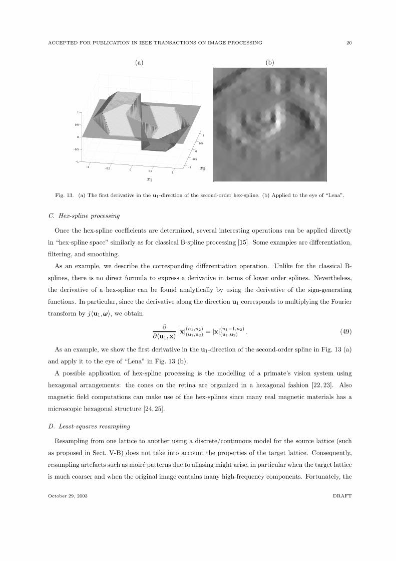
Fig. 13. (a) The first derivative in the u1-direction of the second-order hex-spline. (b) Applied to the eye of “Lena”.

C. Hex-spline processing

Once the hex-spline coefficients are determined, several interesting operations can be applied directly

in “hex-spline space” similarly as for classical B-spline processing [15]. Some examples are differentiation,

filtering, and smoothing.

As an example, we describe the corresponding differentiation operation. Unlike for the classical B-

splines, there is no direct formula to express a derivative in terms of lower order splines. Nevertheless,

the derivative of a hex-spline can be found analytically by using the derivative of the sign-generating

functions. In particular, since the derivative along the direction u1 corresponds to multiplying the Fourier

transform by j〈u1,ωωω〉, we obtain

∂

∂〈u1,x〉|x|(n1,n2)

(u1,u2)= |x|(n1−1,n2)

(u1,u2). (49)

As an example, we show the first derivative in the u1-direction of the second-order spline in Fig. 13 (a)

and apply it to the eye of “Lena” in Fig. 13 (b).

A possible application of hex-spline processing is the modelling of a primate’s vision system using

hexagonal arrangements: the cones on the retina are organized in a hexagonal fashion [22, 23]. Also

magnetic field computations can make use of the hex-splines since many real magnetic materials has a

microscopic hexagonal structure [24, 25].

D. Least-squares resampling

Resampling from one lattice to another using a discrete/continuous model for the source lattice (such

as proposed in Sect. V-B) does not take into account the properties of the target lattice. Consequently,

resampling artefacts such as moire patterns due to aliasing might arise, in particular when the target lattice

is much coarser and when the original image contains many high-frequency components. Fortunately, the



Fig. 14. To demonstrate the principle of resampling by the least-squares approach, consider the rectangular source lattice

(Voronoi cell on the left) and the coarser hexagonal target lattice (Voronoi cell on the right).

use of spline models allows to elegantly incorporate information of the target lattice as proposed in [26].

We briefly describe here how this procedure can be extended to resample between two-dimensional periodic

lattices in general.

Suppose that we have appropriate spline models, both for the source and the target lattice (which might

be either orthogonal or hexagonal). We denote quantities related to the target lattice by an accent:

S(ηp) =

s(x)

∣∣∣∣∣ s(x) =∑

k

c(k)ηp(x−Rk)

,

S(ηp) =

s(x)

∣∣∣∣∣ s(x) =∑

k

c(k)ηp(x− Rk)

.

Now, we want to determine the spline coefficients c(k) on the target lattice, such that the squared error

between both signal representations s(x) and s(x) (in the continuous domain) becomes minimal. This

can be accomplished with the following algorithm, which is an adaptation of the algorithm in [26] for a

hexagonal lattice.

• Determine the spline coefficients c(k) on the source lattice by the direct spline transform, i.e., prefiltering

by (hp)−1.

• Resample the spline coefficients c(k) to

d(k) =∑

l

c(l)ξ(Rk−Rl), (50)

with ξ(x) = ηp ∗ ηp(x)/ det(R).

• Obtain the spline coefficients c(k) on the target lattice by post-filtering with (h2p)−1.

This algorithm can be used to resample between hexagonal lattices or to/from hexagonal and rectangular

lattices. In general, the function ξ(x) can be quite cumbersome to determine analytically, but in practice

it can be approximated numerically. For example, consider resampling from a rectangular lattice to a

much coarser hexagonal lattice. The corresponding Voronoi cells are shown in Fig. 14. Figures 15 (a)

and (b) depict the functions ξ(x) for first and second order. For the first order (p = 1), no pre- or

post-filters are required. For the second order (p = 2), only the post-filter is required and is identical



(a) (b)

−2

−1

0

1

2

−2

−1

0

1

20

0.1

0.2

x1x2 −3

−2−1

01

23

−3

−2

−1

0

1

2

30

0.1

0.2

x1x2

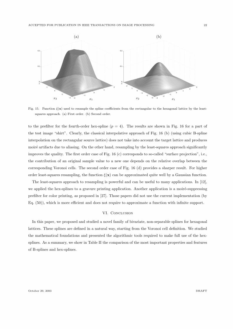
Fig. 15. Function ξ(x) used to resample the spline coefficients from the rectangular to the hexagonal lattice by the least-

squares approach. (a) First order. (b) Second order.

to the prefilter for the fourth-order hex-spline (p = 4). The results are shown in Fig. 16 for a part of

the test image “shirt”. Clearly, the classical interpolative approach of Fig. 16 (b) (using cubic B-spline

interpolation on the rectangular source lattice) does not take into account the target lattice and produces

moire artifacts due to aliasing. On the other hand, resampling by the least-squares approach significantly

improves the quality. The first order case of Fig. 16 (c) corresponds to so-called “surface projection”, i.e.,

the contribution of an original sample value to a new one depends on the relative overlap between the

corresponding Voronoi cells. The second order case of Fig. 16 (d) provides a sharper result. For higher

order least-squares resampling, the function ξ(x) can be approximated quite well by a Gaussian function.

The least-squares approach to resampling is powerful and can be useful to many applications. In [12],

we applied the hex-splines to a gravure printing application. Another application is a moire-suppressing

prefilter for color printing, as proposed in [27]. Those papers did not use the current implementation (by

Eq. (50)), which is more efficient and does not require to approximate a function with infinite support.

VI. Conclusion

In this paper, we proposed and studied a novel family of bivariate, non-separable splines for hexagonal

lattices. These splines are defined in a natural way, starting from the Voronoi cell definition. We studied

the mathematical foundations and presented the algorithmic tools required to make full use of the hex-

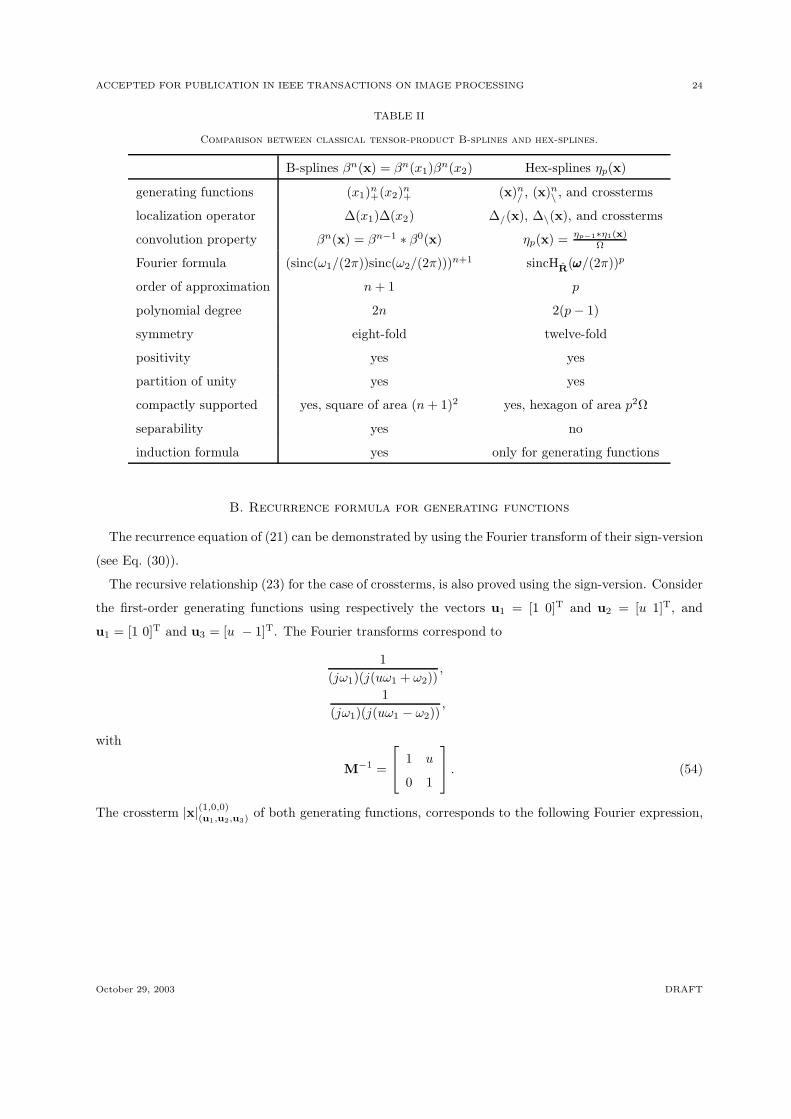
splines. As a summary, we show in Table II the comparison of the most important properties and features

of B-splines and hex-splines.



(a) (b)

(c) (d)

Fig. 16. (a) Part of the test image “shirt”. (b) Result after resampling using the interpolative approach (cubic B-spline

interpolation on the source lattice). (c) Results after resampling using the least-squares approach, first order (p = 1).

(d) Results after resampling using the least-squares approach, second order (p = 2).

Appendices

A. Poisson sum formula

To derive the Poisson sum formula for a hexagonal lattice, we start with the classical formula for an

orthogonal lattice with k ∈ Z2:

∑

k

f(x− k) =∑

k

f(2πk) exp(j2π〈k,x〉). (51)

Introducing the function f(x) = g(Rx), we obtain

∑

k

g(Rx−Rk) =1

|det(R)|∑

k

g(2πRk) exp(j2π〈k,x〉). (52)

Finally, we substitute Rx = y, which yields the Poisson sum formula for an hexagonal lattice:

∑

k

g(y −Rk) =1

|det(R)|∑

k

g(2πRk) exp(j2π⟨RTk,y

⟩). (53)



TABLE II

Comparison between classical tensor-product B-splines and hex-splines.

B-splines βn(x) = βn(x1)βn(x2) Hex-splines ηp(x)

generating functions (x1)n+(x2)

n+ (x)n

/ , (x)n\ , and crossterms

localization operator ∆(x1)∆(x2) ∆/(x), ∆\(x), and crossterms

convolution property βn(x) = βn−1 ∗ β0(x) ηp(x) =ηp−1∗η1(x)

Ω

Fourier formula (sinc(ω1/(2π))sinc(ω2/(2π)))n+1 sincHR

(ωωω/(2π))p

order of approximation n + 1 p

polynomial degree 2n 2(p− 1)

symmetry eight-fold twelve-fold

positivity yes yes

partition of unity yes yes

compactly supported yes, square of area (n + 1)2 yes, hexagon of area p2Ω

separability yes no

induction formula yes only for generating functions

B. Recurrence formula for generating functions

The recurrence equation of (21) can be demonstrated by using the Fourier transform of their sign-version

(see Eq. (30)).

The recursive relationship (23) for the case of crossterms, is also proved using the sign-version. Consider

the first-order generating functions using respectively the vectors u1 = [1 0]T and u2 = [u 1]T, and

u1 = [1 0]T and u3 = [u − 1]T. The Fourier transforms correspond to

1

(jω1)(j(uω1 + ω2)),

1

(jω1)(j(uω1 − ω2)),

with

M−1 =

1 u

0 1

. (54)

The crossterm |x|(1,0,0)(u1,u2,u3)

of both generating functions, corresponds to the following Fourier expression,



which can be separated using partial fractions and ζ = ω2/uω1:

1

(jω1)2(j(uω1 + ω2))(j(uω1 − ω2))

=1

(jω1)2(juω1)2(1 + ζ)(1 − ζ)

=1

2(jω1)2(juω1)2

(1

1 + ζ+

1

1− ζ

)

=1

2〈u1,u2〉(jω1)3

(1

(j(uω1 + ω2))+

1

(j(uω1 − ω2))

),

which gives us

|x|(1,0,0)(u1,u2,u3)

=1

2〈u1,u2〉(|x|(2,0)

(u1,u2)+ |x|(2,0)

(u1,u3)

).

Applying this equation to a general crossterm results in Eq. (23).

This recursive equation can also be used to compute some derivative generating functions. For example,

when computing the derivative in the direction of u2, the Fourier transform of one of the generating

functions can get a (j〈u2,ωωω〉) in the nominator. This can be undone by applying

(x)(n1+1,n2−1,n3)(u1,u2,u3)

= 2〈u1,u2〉(x)(n1,n2,n3)(u1,u2,u3)

− (x)(n1+1,n2,n3−1)(u1,u2,u3)

.

C. Localization of two-sided generating functions

We briefly show how the sign-version of |x|0(u1,u2)= |x|0/ gets localized by ∆/. We start with the

following lemma.

Lemma 1: Given a one-sided generating function (x)0(u1,u2)and the corresponding ∆/, we have:

∆/ ∗ (x)0(−u1,u2)= −∆/ ∗ (−x)0(u1,u2)

, (55)

∆/ ∗ (x)0(u1,−u2)= −∆/ ∗ (x)0(u1,u2)

. (56)

Proof: The Fourier transforms of the one-sided generating functions (x)0(−u1,u2)and −(−x)0(u1,u2)

are

respectively

(x)0(−u1,u2)←→

( −1

j〈ωωω,u1〉+ πδ(〈ωωω,u1〉)

)(1

j〈ωωω,u2〉+ πδ(〈ωωω,u2〉)

)

=1

〈ωωω,u1〉〈ωωω,u2〉− πδ(〈ωωω,u2〉)

j〈ωωω,u1〉+

πδ(〈ωωω,u1〉)j〈ωωω,u2〉

+ π2δ(〈ωωω,u1〉)δ(〈ωωω,u2〉),

−(−x)0(u1,u2)←→ 1

〈ωωω,u1〉〈ωωω,u2〉+

πδ(〈ωωω,u2〉)j〈ωωω,u1〉

+πδ(〈ωωω,u1〉)

j〈ωωω,u2〉− π2δ(〈ωωω,u1〉)δ(〈ωωω,u2〉).

Using this result, the remaining terms of the difference between the right and left hand side of Eq. (55)

can be “neutralized” using the localization of δ(〈ωωω,u2〉), which equals zero:

∆/(ωωω)δ(〈ωωω,u2〉) = ∆(〈ωωω, e1 + e2〉)∆(〈ωωω, e1 − e2〉)δ(〈ωωω,u2〉)

= ∆(〈ωωω, e1 + e2〉) ∆(〈ωωω, λu2〉)δ(〈ωωω,u2〉)︸︷︷︸0

= 0,



where λ = −⟨e2 − e1, [0 1]T

⟩, according to the definition of u2.

Next, we write the two-sided generating function |x|0/ in terms of one-sided generating functions using

Eq. (26) and applying Eqs. (55) and (56):

∆/ ∗ |x|0/ =∆/

4∗((x)0(u1,u2)

− (x)0(u1,−u2)+ (x)0(−u1,−u2)

− (x)0(−u1,u2)

)

=∆/

2∗((x)0(u1,u2)

+ (−x)0(u1,u2)

)

=∆/

2∗((x)0/ + (−x)0/

). (57)

This corresponds to a symmetrized version of the “intermediate” part of the hex-spline (this can easily

checked by applying the construction algorithm of Sect. III-B to (−x)0/). Analogously we can obtain

∆\ ∗ |x|0\ =∆\2∗((x)0\ + (−x)0\

). (58)

Adding up both parts, i.e., Eqs. (57) and (58), results into the first-order hex-spline.

D. Implementation: the analytical form

To obtain the analytical expression of the hex-splines it is safer to rely on a mathematical soft-

ware package for symbolic manipulations. We have made an implementation available for Maple at

http://bigwww.epfl.ch/demo/hexsplines/. This software is also able to obtain the analytical form of

irregular hex-splines, using the same construction technique as explained in this article. In particular,

we assume the following lattice matrix R is given, corresponding to the general class of semi-regular

hexagonal lattices of the second type [14]:

R =

b 0

−a2 a

, (59)

with 2b > a > 0. The values a and b can be passed to the program. Hexagonal lattices of the first type

can easily be obtained by exchanging x1 and x2.

The package makes use of two auxiliary functions:

• hexlocalization: Computes the localization operator given the vectors e1, e2, e3. The arguments k1

and k2 indicate the power to which both localization operators are raised.

• hexbuilding: Computes a generating function given the vectors u1, u2, u3. The argument pow is a

vector containing the powers (n1, n2, n3) of a general term. In the implementation, the powers correspond

to the powers of the Fourier terms. The coordinates xc1 and xc2 are used for the Heaviside terms which

delineate the support of the generating functions. This allows us to compute the analytical form inside a

triangular patch of the hex-splines.

These auxiliary functions are called by the main routine diffhexspline that composes a general hex-

spline with lattice parameters a and b, a given order, and eventually derivatives in one of the three



(a) (b) (c)

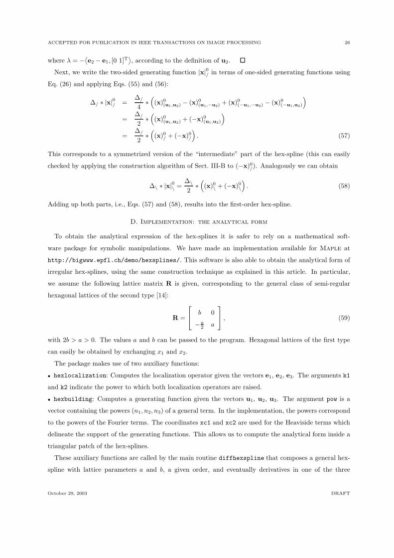
Fig. 17. (a) A square image, sampled on a hexagonal lattice, is embedded by a rectangular support. The light gray regions

are redundant. (b) An example for the test image “Lena”, mirror boundary conditions are applied. (c) The test image

“Lena” in the integer coordinate system (k1, k2).

main directions. The other functions initialize some parameters for common cases: hexspline omits the

derivative, diffrhexspline is for a regular hex-spline, and rhexspline computes the regular hex-spline

without derivatives.

E. Implementation: the direct spline transform

The direct spline transform computes the spline coefficients for a hex-spline representation given the

sample values. As shown in Sect. IV-D, this corresponds to the inverse filter operation of the corresponding

discrete hex-spline. For one-dimensional B-splines (and higher-dimensional versions by the tensor-product

extension), a fast recursive algorithm exists [28]. Unfortunately, the discrete hex-splines cannot be sep-

arated in a series of causal and anti-causal recursive filters. In this paper, we propose an equivalent

implementation of the inverse filter in Fourier domain by 1/hp(ωωω).

There are two approaches to compute the Fourier coefficients of samples taken on a hexagonal grid.

First, one can make use of a true hexagonal discrete Fourier transform [29,30]. Second, the hexagonal data

is embedded in a rectangular support spanned by the lattice vectors, i.e., the index [k1k2]T (0 ≤ k1 < N1,

0 ≤ k2 < N2) relates to k1r1 + k2r2. Here, we have preferred the second approach which can make use of

widely available FFT-algorithms on a rectangular lattice. First, the data is embedded as shown in Fig. 17.

Regions outside the support of the original image is extended by mirror boundary conditions. The result,

i.e., the image of Fig. 17 (c), is indexed as gR(k) = g(Rk). Next, the Fourier coefficients is computed by



a regular FFT-algorithm. Taking into account Eqs. (3) and (44), filtering needs to be done by

|det(R)|hp(R−Tn)

, (60)

where n = [n1/N1 n2/N2]T, 0 ≤ n1 < N1, 0 ≤ n2 < N2. Finally, the inverse FFT provides the spline

coefficients.

Acknowledgments

The authors would like to express their gratitude to the anonymous reviewers for their valuable remarks

that have contributed to the final quality of this paper.

This work was partially supported by the FWO (Fund for Scientific Research - Flanders, Belgium),

through a mandate of Research Assistant (Dimitri Van De Ville).

References

[1] D.P. Petersen and D. Middleton, “Sampling and reconstruction of wave-number-limited functions in N-dimensional

Euclidean spaces,” Information and control, vol. 5, pp. 279–323, 1962.

[2] R.M. Mersereau, “The processing of hexagonally sampled two-dimensional signals,” Proceedings of the IEEE, vol. 67,

no. 6, pp. 930–949, June 1979.

[3] R.M. Mersereau, “Two-Dimensional Nonrecursive Filter Design,” Topics in Applied Physics: Two-Dimensional Digital

Signal Processing I, vol. 42, 1981.

[4] Wenzhe Li and Alfred Fettweis, “Interpolation filters for 2-D hexagonally sampled signals,” International Journal of

Circuit Theory and Applications, vol. 25, pp. 259–277, 1997.

[5] M. J. E. Golay, “Hexagonal parallel pattern transformations,” IEEE Transactions on Computers, vol. C-18, no. 8, pp.

733–740, Aug. 1969.

[6] Richard C. Staunton, “The design of hexagonal sampling structures for image digitisation and their use with local

operators,” Image and Vision Computing, vol. 7, no. 3, pp. 162–166, 1989.

[7] Lee Middleton and Jayanthi Sivaswamy, “Edge detection in a hexagonal-image processing framework,” Image and

Vision Computing, vol. 19, no. 14, pp. 1071–1081, Dec. 2001.

[8] A. Laine and S. Schuler, “Mammographic feature enhancement by multiscale analysis,” IEEE Transactions on Medical

Imaging, vol. 13, no. 4, pp. 725–740, Dec. 1994.

[9] A. P. Fitz and R. J. Green, “Fingerprint classification using a hexagonal fast fourier transform,” Pattern Recognition,

vol. 29, no. 10, pp. 1587–1597, 1996.

[10] Senthil Periaswamy, “Detection of microcalcifications in mammograms using hexagonal wavelets,” M.S. thesis, Univer-

sity of South Carolina, 1996.

[11] R. C. Staunton, “One-pass parallel hexagonal thinning algorithm,” IEE Proc. Vision, Image and Signal Processing,

vol. 148, no. 1, pp. 45–53, 2001.

[12] Dimitri Van De Ville, Wilfried Philips, and Ignace Lemahieu, “Least-squares spline resampling to a hexagonal lattice,”

Signal Processing: Image Communication, vol. 17, no. 5, pp. 393–408, May 2002.

[13] Eric Dubois, “The sampling and reconstruction of time-varying imagery with application in video systems,” Proceedings

of the IEEE, vol. 73, no. 4, pp. 502–522, Apr. 1985.

[14] Robert A. Ulichney, Digital Halftoning, MIT Press, 1987.

[15] Michael Unser, Akram Aldroubi, and Murray Eden, “B-spline signal processing,” IEEE Transactions on Signal

Processing, vol. 41, no. 2, pp. 821–848, Feb. 1993.

[16] C. de Boor, K. Hollig, and S. Riemenschneider, Box splines, vol. 98 of Applied Mathematical Sciences, Springer-Verlag,

1993.



[17] C. de Boor and K. Hollig, “B-splines from parallelepipeds,” J. Analyse Math., , no. 42, pp. 99–115, 1982.

[18] Paul Sablonniere and Driss Sbibih, “B-splines with hexagonal support on a uniform three-direction mesh of plane,” C.

R. Acad. Sci. Paris, vol. 319, no. I, pp. 277–282, 1994.

[19] Thierry Blu and Michael Unser, “Quantitative Fourier analysis of approximation techniques: Part I—interpolators and

projectors,” IEEE Transactions on Signal Processing, vol. 47, no. 10, pp. 2783–2795, Oct. 1999.

[20] Marc Tremblay, Stephane Dallaire, and Denis Poussart, “Low level segmentation using CMOS smart hexagonal image

sensor,” in Proceedings of the Conference on Computer Architectures for Machine Perception. 1995, pp. 21–28, IEEE.

[21] Stefan Jung, Roland Thewes, Thomas Scheiter, Karl F. Goser, and Werner Weber, “Low-power and high-performance

CMOS fingerprint sensing and encoding architecture,” IEEE Journal of Solid State Circuits, vol. 34, no. 7, pp. 978–984,

July 1999.

[22] D.H. Mugler and M. D. Ross, “Vestibular receptor cells and signal detection: Bioaccelerometers and the hexagonal

sampling of two-dimensional signal,” Mathematical and Computer Modelling, vol. 13, no. 2, pp. 85–92, 1990.

[23] Brian A. Wandell, Foundations of Vision, Sinauer Associates, 1995.

[24] M. Mansuripur and R. Giles, “Demagnetizing fields computation for dynamic simulation of the magnetization reversal

process,” IEEE Transactions on Magnetics, vol. 24, no. 1, pp. 23–27, Jan. 1988.

[25] R. Giles, P. R. Kotiuga, and M. Mansuripur, “Parallel micromagnetic simulations using fourier methods on a regular

hexagonal lattice,” IEEE Transactions on Magnetics, vol. 27, no. 9, pp. 3815–3818, Sept. 1991.

[26] M. Unser, A. Aldroubi, and M. Eden, “Enlargement or reduction of digital images with minimum loss of information,”

IEEE Transactions on Image Processing, vol. 4, no. 3, pp. 247–258, Mar. 1995.

[27] Dimitri Van De Ville, Wilfried Philips, Ignace Lemahieu, and Rik Van de Walle, “Suppression of sampling moire in

color printing by spline-based least-squares prefiltering,” Pattern Recognition Letters, vol. 24, no. 11, pp. 1787–1794,

July 2002.

[28] M. Unser, “Fast B-spline transforms for continuous image representation and interpolation,” IEEE Transactions on

Pattern Analysis and Machine Intelligence, vol. 13, no. 3, pp. 277–285, Mar. 1991.

[29] James C. Ehrhardt, “Hexagonal fast fourier transform with rectangular output,” IEEE Transactions on Signal Pro-

cessing, vol. 41, no. 3, pp. 1469–1472, Mar. 1993.

[30] A. M. Grigoryan, “Efficient algorithms for computing the 2-D hexagonal fourier transforms,” IEEE Transactions on

Signal Processing, vol. 50, no. 6, pp. 1438–1448, June 2002.


hex-splines: a novel spline family for hexagonal latticesbig · a novel spline family for hexagonal...

Documents