Hi-Stat

Discussion Paper Series

No.132

Real GDP in Pre-War East Asia: A 1934-36 Benchmark Purchasing

Power Parity Comparison with the U.S.

Kyoji Fukao, Debin Ma and Tangjun Yuan

January 2006

Hitotsubashi University Research Unit for Statistical Analysis in Social Sciences

A 21st-Century COE Program

Institute of Economic Research

Hitotsubashi University Kunitachi, Tokyo, 186-8603 Japan

http://hi-stat.ier.hit-u.ac.jp/

Real GDP in Pre-War East Asia: A 1934-36 Benchmark Purchasing Power Parity Comparison with the U.S.

Kyoji Fukao Institute of Economic Research

Hitotsubashi University

*Debin Ma (corresponding author) Economic History Department, London School of Economics, U.K;

and National Graduate Institute for Policy Studies, Tokyo, Japan.

Tangjun Yuan

Institute of Economic Research Hitotsubashi University

Jan. 2006

Abstract This article provides estimates of purchasing power parity (PPP) converters for expenditure side GDP of Japan/China and Japan/U.S through a detailed matching of prices for more than 50 types of goods and services in private consumption and about 20 items or sectors for investment and government expenditure. Based on our finding and linking with the earlier studies on the relative price levels of Taiwan and Korea, we derive the mid-1930s benchmark PPP adjusted per capita income of Japan, China, Taiwan and Korea at 31%, 10%, 23%, and 12% of the U.S. level respectively for the mid-1930s. These estimates corrected the consistent downward bias in East Asian income levels based on market exchange rate conversions. While confirming Angus Maddison’s estimates for China and Taiwan based on the 1990 benchmark back-projection method, they do point to a 23% and 85% overestimate in his comparable figures for Japan and Korea respectively for the mid-1930s period. This article develops a preliminary theoretical and empirical framework to demonstrate the possible source of the biases in the back-projection method. We briefly discuss the implications of our findings on the initial conditions and long-term growth dynamics in East Asia and beyond. *Please direct all correspondence to Debin Ma, Economic History Department, London School of Economics, Houghton Street, London, WC2A, 2AE. Email: d.ma1@lse.ac.uk or debinma@hotmail.com. We are grateful for Paul Rhode and John Devereux for pointing to us useful data sources. We thank Angus Maddison, Hak Kil Pyo, Jean Pascal Bassino, Prema-Chandra Athukorala, Konosuke Odaka and the participants of the UC Davis workshop “Estimating Production and Income Across Nations and over Time” held on May 31 – June 1, 2005. This paper is partly funded by the NSF “Global Prices and Income 1350-1950” project headed by Peter Lindert at UC Davis and the Ministry of Education 21st Century COE Program, “Research Unit for Statistical Analysis in Social Sciences,” headed by Osamu Saito at Hitotsubashi University. All errors are the responsibility of the authors.

2

Real GDP in Pre-War East Asia:

a 1934-36 Benchmark Purchasing Power Parity Comparison with the U.S.

Abstract: This article provides estimates of purchasing power parity (PPP) converters for expenditure side GDP of Japan/China and Japan/U.S through a detailed matching of prices for more than 50 types of goods and services in private consumption and about 20 items or sectors for investment and government expenditure. Based on our finding and linking with the earlier studies on the relative price levels of Taiwan and Korea, we derive the mid-1930s benchmark PPP adjusted per capita income of Japan, China, Taiwan and Korea at 31%, 10%, 23%, and 12% of the U.S. level respectively for the mid-1930s. These estimates corrected the consistent downward bias in East Asian income levels based on market exchange rate conversions. While confirming Angus Maddison’s estimates for China and Taiwan based on the 1990 benchmark back-projection method, they do point to a 23% and 85% overestimate in his comparable figures for Japan and Korea respectively for the mid-1930s period. This article develops a preliminary theoretical and empirical framework to demonstrate the possible source of the biases in the back-projection method. We briefly discuss the implications of our findings on the initial conditions and long-term growth dynamics in East Asia and beyond.

In the world history of modern economic growth, the East Asian miracle is a relatively recent

phenomenon. The catch-up of Japan, Taiwan and Korea with the world’s leading economies is a 20th century –

or to be more precise – a post-WWII affair, while the economic surge of China is even more recent, occurring

during the last two decades. However, as revealed by the burgeoning literature on economic growth, long-term

or historical factors provide us with crucial insights into both the causal determinants and the mechanism of

modern economic growth. What were the initial conditions of East Asian economies prior to their take-off?

Were there shared vital historical factors behind their miracles?

These questions cannot be properly answered without long-term series of national accounts. Among the

East Asian economies, the most consistent and reliable long-term GDP series going back to the late-19th

century are available only for Japan, partly thanks to the efforts of the Long-Term Economic Statistics (LTES)

project under the leadership of Kazushi Ohkawa at the Institute of Economic Research of Hitotsubashi

University in Japan.1 The Hitotsubashi group extended this line of research to two former Japanese colonies,

Taiwan and Korea, with the 1988 publication of a statistical volume compiled by Mizoguchi and Umemura.

The volume provides annual estimates of GDP and its various components for these two economies during the

period of Japanese occupation based on the detailed economic statistics of the colonial administrations.

Compared with these countries, historical macroeconomic statistics for China remain sketchy. The earliest set

of economic statistics approaching standard national accounts data are for the 1930s, laying the foundation for

1 For Japan, there is the 14 volume LTES publication in Japanese. For an abridged English version, see the volume by Kazushi Ohkawa and Miyohei Shinohara.

3

the pioneering reconstruction of China’s GDP for the period 1931-36 carried out by Ou et al. (1947), Liu

(1947), and Liu and Yeh (1965).

These pre-war GDP series are all based on their respective currencies, making cross-country

comparisons difficult. Conversion using market exchange rates tends to systematically underestimate the real

per capita income level of lower income countries since it fails to incorporate differences in the price level for

non-tradable goods (Balassa, 1964; Samuelson, 1964). Yet research on the construction of purchasing power

parity (PPP) converters for GDP for the pre-war period, especially for developing countries such as those in

East Asia, is still at a very early stage. The national accounts datasets based on PPP conversion by the

renowned Penn World Table group only cover the post-War period. Angus Maddison is possibly the only

scholar to have attempted a systematic reconstruction of long-term national accounts for most countries around

the world.

To arrive at globally comparable series for the pre-war period, Maddison relied on the use of 1990

benchmark PPPs to project GDP values backward using domestic real GDP growth rates. This methodology,

adopted due to the absence of historical PPP converters, has its inherent index number problems associated

with factors such as long-term relative shifts in a country’s terms of trade and economic structure. Based on a

full-fledged reconstruction of 1934-36 expenditure PPP for Japan, Taiwan and Korea, a recent study by Fukao,

Ma and Yuan (2004) revealed inconsistencies in Maddison’s pre-war per capita GDP estimates for Taiwan and

Korea.

The present paper follows the Fukao, Ma, and Yuan (2006) study on the PPPs of Japan, Taiwan and

Korea and develops a PPP convert first for Japan and China and then for Japan and the U.S. We conduct a

detailed matching of the prices of more than 50 types of goods and services for private consumption and about

20 expenditure items for private investment and government expenditure. We find that average consumer

prices in China in 1934–36 were about 75% of Japan’s, while the average GDP price level in Japan was 44%

that of the U.S. Linking with the Fukao, Ma and Yuan study on the relative price levels of Taiwan and Korea

and using Japan as the bridge country, we derive the mid-1930s benchmark PPP-adjusted per capita income of

Japan, China, Taiwan, and Korea at 31%, 10%, 23%, and 12% of that of the U.S respectively. These figures are

consistently higher than their corresponding per capita GDP estimates based on current market exchange rates,

which are 14%, 3.6%, 9%, and 5.2% of the U.S level respectively.

4

Our results for Taiwan and China are similar to Maddison’s back-projected estimates in 1990 dollars. On

the other hand, our estimate for Korea’s per capita income level is only about half the level estimated by

Maddison. But the differences in our results are most important for our bridge country, Japan. Our current-price

PPP benchmark estimate gives a Japanese per capita income 19% lower than that of Maddison (Maddison 2003,

p.182). In fact, comparing our estimate with the data for other countries provided in Maddison (2003) suggests

that Japan’s per capita income during this period was only marginally higher than those of Malaysia or the

Philippines. Thus, it is interesting to note that Japan launched her full military venture on the Asian continent

with a per-capita income roughly comparable to some of the resource-rich Asian countries, most of which were

still Western colonies. If we project backward or forward from our benchmark PPP estimates, our study sheds

new light on the initial conditions of Japan and East Asia both around the mid-19th century and the post-WWII

period. We offer some explorations on the growth implications of our estimates.

The remainder of this paper is divided into three sections followed by a conclusion. The first section

provides a detailed explanation of our PPP estimation procedure. We also report our findings on current-price

PPP estimates in 1934–36. In Section II we present our new estimates of per capita incomes in the four East

Asian economies with the U.S. We also compare our current price PPP based per capita income estimates with

those based on current market exchange rates as well as the backward projection estimates. Section III

discusses the index number biases embedded in the back-projection method. The concluding section provides a

brief discussion of our reassessment of initial conditions and long-term growth dynamics in East Asia based on

our new findings.

I. Current-Price PPP Estimates for 1934–36

PPP Converter for Private Consumption: Japan and China

We adopt the methodology used by several rounds of the International Comparison Program (ICP) for

the post-WWII benchmark periods.2 We choose the 1934–36 period as our benchmark for several reasons.

First, this period has been consistently used as the benchmark in the LTES project. Second, for Japan and her

two former colonies, 1934–36 was a period of relative economic and price stability, falling between the severe

deflation that lead to Japan’s banning of gold exports in 1931–32 and the economic dislocation of the late

2 For the ICP study, see Heston and Summers 1993 and Maddison 1995

5

1930s brought about by the outbreak of the Sino-Japanese War. In China, there was a major monetary reform

by the Nationalist government in 1933 which succeeded in replacing the traditional silver-based monetary

system with a modern unified currency under the control of a Central Bank. More importantly, for the 1931–36

period, we have the first reasonably reliable benchmark GDP estimate. Finally, for East Asia in general, it was

only during the 1930s that urban and rural household surveys became much more plentiful and reliable.

Our computation of relative price levels employs the standard binary matching of two countries. We

derived the Fisher geometric mean as follows. For N number of goods and services, the price level in yen of the

numeraire country (sub- or superscripted as J here) relative to the price level in Japanese yen of country i is

calculated as follows:

where pin denotes absolute price level of commodity (or service) n in country i in Japanese yen in the period of

1934-36. The summation sign is summed across all the types of goods and services. We use the average market

exchange rate in 1934-36 for conversion of absolute price levels between coutry i’s currency and Japanese yen.

The formula using the consumption weight of country i is:

iJiP ,

∑∑∑

∑∑ ===

ini

n

Jni

nini

n

Jn

in

in

in

Jn

in

in

ppqp

pp

qpqpqp

ω

1

Finally, the geometric average of the two price indices (the Fisher index) JJi

iJiJi PPP ,,, ×= gives us country

i’s absolute price level relative to that of Japan.

The information on prices and expenditure weights for Japan is based on the earlier PPP studies on Japan,

Taiwan and Korea (Yuan and Fukao, 2002; Fukao, Ma, and Yuan, 2004). Prices for each item in Japan in most

cases are calculated as the simple average of the retail price in 12 to 14 major cities.

Our current-price PPP estimate for China and Japan draws on Yuan (2005). For China, we rely on more

than 60 volumes of detailed retail price statistics compiled in 1955 by the Communist government. The

∑∑∑

∑∑ === J

nJn

in

Jn

Jn

Jn

JnJ

n

in

Jn

Jn

Jn

inJ

Ji pp

qp

qppp

qpqp

P ω,

6

volumes are titled “Gongnongye Shangping Bijia Wenti Diaocha Yanjiu Ziliaoji (Archive Materials for Studies

of Industrial and Agricultural Commodity Prices).” The retail price information in these volumes is mostly

culled from the account books of major stores in urban cities. The price statistics were published and circulated

internally within the Chinese government and were intended for studying changes in relative prices between

agriculture and industry between the 1930s the 1950s. Our retail prices used are the simple averages of the

cities of Shanghai, Chongqing, Wuhan, Guangzhou, Beijing, Nanjing, Haerbin, Xining, Shijiazhuang

Zhengzhou, Erjiazhen and Tianjin. For some of the services, such as electricity, movies, and so on, Yuan

(2005) gathered information from local surveys and newspapers such as “Sichuan Jingji Cankao Ziliao” and

“Dakong News.”

We employ three levels of consumption weights. The consumption weights at the aggregate level come

from Zhang Donggang (2001, pp.375-6), with some adjustments. For medium and detailed level weights, we

use various local surveys divided into an urban and a rural group, with urban and rural weights derived by their

respective population figures. In the case of food consumption, we use urban consumption surveys for

Shanghai, Tianjin, Nanjing, Wuxi and rural surveys for Beijing, Dingxian, Jiangning, Wuxing, Yuliangzhuang,

Shangxiawuzhen, Xianghu and Wujiang.

The details of the matching and data sources for China-Japan PPP converter for consumption are

presented in Appendix Table I which shows a matching of 51 items. Table 1 shows the summary information

that gives an overall relative price level of China at 75% that of Japan. Among the five categories, Chinese

food prices were the lowest of all. Another notable feature from the table is the large discrepancy between the

relative price levels of lighting and heat based on Chinese expenditure weights and Japanese expenditure

weight (0.411 versus 1.363, also see Appendix Table I). The disparity is a reflection of China’s very low rates

of electrification and relatively high cost of electric power in comparison to that of Japan, a powerful indicator

of the differential degree of economic modernization between these two countries for the period.3

Insert Table 1

PPP Converter for Private Consumption: Japan and the United States

3 Total electric power generated in Japan is more than 10 times of that in China (excluding Japanese-controlled Manchuria) in the 1930s. For total electric power generated in Japan and China in the 1930s, see Minami Ryoshin (1965) and Wang Qingyi (1988) respectively.

7

Price data for the U.S. in the mid-1930s are fairly abundant and reliable. For most of the food items, we

rely on the Bureaus of Labor Statistics Bulletin No. 635 which provides weighted averages of retail prices in 51

cities in the U.S. For the retail prices of fuel and utilities as well as wage rates, we used the Handbook of Labor

Statistics (1941). Other sources include the Statistical Abstract of the United States (1938) for wholesale prices

for a few items such as clothing and utilities, and micro data from a comprehensive national urban household

survey of consumer purchases in 1935–36. This household-based dataset can now be accessed through the

ICPSR website hosted by the University of Michigan (http://www.icpsr.umich.edu).

The Historical Statistics of the U.S (bicentennial edition) provide us with the upper and medium

consumption expenditure weights. The detailed item weights in the mid-1930s largely draw from the cost of

living survey in Bureau of Labor Statistics publication (Bulletin no. 699).

Details of the matching are presented in Appendix Table II. Table 2 summarizes our U.S-Japan binary

matching of 53 items of goods and services altogether. It shows that around the mid-1930s the average cost of

food in Japan was about half of that in the United States. On the other hand, the average cost of miscellaneous

items in Japan, consisting mostly of services such as transportation, communication, education and

entertainment, was only 37% of the U.S. level. In the case of lighting and heating which are mostly energy

items, the Japanese price level was identical to the U.S level. Housing expenses, which include the rent of land

– a scarce factor in Japan – were about 63% of the U.S level. The overall relative price level of Japan relative to

the U.S. turns out to be 46% for the mid-1930s benchmark.

Insert Table 2

It is also instructive to look at the relative price structures of the U.S and Japan shown in Table 2 and

Appendix Table II. For example, Appendix Table II suggests that Japanese nominal wage rates in most sectors

were only about 10% the U.S. level based on mid-1930s exchange rates. The low wages and high energy and

housing prices in Japan reflect differences in resource endowments and possibly productivity levels during this

period.

The study by Fukao, Ma and Yuan (2006) matched 61 types of goods and services for the Japan-Korea

comparison and 58 items for the Japan-Taiwan comparison. We can combine the consumption PPPs from that

study with our current result on China/Japan and Japan/US to convert all our relative price levels to the basis of

the U.S by using Japan as the bridge country. Again, Fisher averages are applied across the five upper level

8

consumption weights over the binary-matching of these four East Asian economies with the U.S. The results

are presented in Table 3 which indicates that the price levels of China, Taiwan, Korea and Japan relative to the

United States stood at 34%, 39%, 44%, and 46% respectively. Overall, price levels in East Asia were far lower

in comparison with the U.S than within the region. Within East Asia, price levels within the Japanese colonial

empire were closer to each other than with China, a fact consistent with Japan’s colonial policy which forged a

“free trade” zone within the empire by the 1930s.4

Insert Table 3

Table 3 also shows that overall price gaps for non-tradables between East Asia and the U.S are larger

than those for tradables. This is a clear confirmation of the theoretical predictions of the productivity and factor

proportion differential models that posit lower price levels for non-tradables in relatively underdeveloped

countries. As is well known, using market exchange rates ignores the lower prices – particularly of non-

tradables – and thus underestimates the per capita income levels of less developed countries. The ranking of

relative price levels presented in Table 3 is consistent with their per capita income rankings relative to the

United States, which we will show later.

In Table 4, we present the aggregate five-item upper level consumption expenditure weights. The table

shows that the consumption expenditure patterns of China and Korea during that period were roughly

comparable, while those of Taiwan and Japan, exhibiting the most “advanced” pattern with the lowest share in

food items, had much in common with the U.S.

Insert Table 4

PPP Converter for Private Investment and Government Expenditures: Japan and the United States

Expenditure side GDP consists of private consumption, investment, government expenditure, and net

exports. In this section, we follow the standard practice of the International Comparison Projects (ICP) to

estimate the other two components of GDP, private investment and government expenditure.5 For China,

4 Taiwan and Korea became Japanese colonies in 1895 and 1910, respectively. By the 1910s, both Korea and Taiwan were set on a de-facto “Japanese yen exchange standard,” – the two Central banks, the Bank of Korea and the Bank of Taiwan, issued their bank notes as circulating currency convertible to the Bank of Japan notes which served as the de-facto reserve currency. The currencies of Taiwan and Korea were also yen. The currencies of the three countries were convertible at the 1:1 exchange rate. By the 1930s, Taiwan, Korea and Japan had moved towards a free trade bloc protected by a common external tariff (Yamamoto 2000). 5 As consistent with ICP and other international comparison studies, we do not separately estimate PPP for net exports partly because their share are likely to be small as a per cent of total GDP (especially for large countries) and partly because prices of traded goods are already included in other GDP components.

9

relevant data for investment and government expenditure are unavailable. Liu and Yeh (1965, p. 68) indicated

that private consumption accounted for 91% of Chinese GDP during the benchmark period. We therefore feel

reasonably comfortable to use our consumption PPP as a proxy for our GDP PPP in this study.

Due to data limitation, our estimates of PPP converters for private investment and government

expenditures for Japan-U.S have to rely on somewhat crude assumptions. For estimation of PPP converter for

private investment, we examine relative price levels of two main categories of private investment: equipment

and construction investment in Japan and the United States. In the case of equipment investment, we use the

relative price level calculated by Pilat (1993) for machinery and equipment for 1939. In the case of construction

investment, we derive the price levels in Japan and the United States as weighted averages of price for

construction materials and wages for construction laborers. The results are presented in Table 5 suggesting that

the price level for private investment is 51% of the U.S. level, higher than the price level for private

consumption.

Insert Table 5

For government expenditure for Japan and the U.S., we divide them into two categories: labor and

material costs. Labor costs are measured as the ratio of the average salary per government employee in Japan

and U.S. Table 6 shows that the average Japanese government employees’ pay was only 7% of their U.S

counterparts’ in nominal terms. The second category, material cost, consists of government purchases from

various sectors of the economy. Table 6 provides relative price levels and expenditure weights of ten materials.

Their relative price level (of Japan over U.S) in weighted average turns out to be 60%, higher than that for

private consumption. This seems plausible as government purchase draws a substantial share from the

investment sector of which Japanese price levels were closer to that in the U.S. Overall, thanks to the much

lower remuneration paid to employees in Japan, the Japanese government expenditure price level overall was

only 30% of that of the U.S.

Insert Table 6

Using the current-price PPP converters for private consumption, private investment, and government

expenditures for Korea and Taiwan (relative to Japan) from Fukao, Ma, and Yuan (2004), and using Japan as

the bridge country, we derive a full set of current-price PPP converters for GDP for the four East Asian

10

economies for the mid-1930s, all converted to the base of the U.S, using the Fisher average. The detail of the

calculation procedures and the results are reported in Table 7.

Insert Table 7

II. East Asian GDPs in the 1930s: an International Comparison

Comparing GDP at PPP and Market Exchange Rates

Table 8 presents the per capita GDP of the four East Asian economies in 1934-36 U.S dollars. The first

data row shows GDP estimates for the different countries in 1934-36 current prices and converted at market

exchange rates. Not surprisingly, GDP at exchange rates gives very low income estimates for East Asia in the

mid-1930s: Japan’s per capita income, according to this method, was only 14% of that of the U.S. while that of

China was a mere 3.6% of the U.S. level. The second row of Table 8 presents the price levels of the four East

Asian economies relative to the U.S derived with Japan as the bridge country.

Insert Table 8

Dividing the exchange rate-based per capita income estimates by the relative price levels, we can derive

our 1934-36 benchmark PPP adjusted estimates, presented in the third row of Table 8. In comparison with the

exchange rate conversion, our PPP converter more than doubles the per capita income of Japan, Korea and

Taiwan and more than triples the per capita income of Taiwan and China. Undoubtedly, our PPP conversion is

a major correction of the downward exchange rate bias.

Existing studies on PPP for the pre-war East Asia are few. The study by Colin Clark published in 1940

(p. 41) gave Japanese per capita income in 1925-34 at about 26% of the U.S level, quite close to our result.

However, since both the GDP estimates and price levels used by Clark were long outdated, his study should not

be viewed as a direct confirmation of our estimates. Nonetheless his results may well reveal the perception of

the time. The more systematic Japan-U.S PPP study was carried out by Pilat (1993, 1994) with 1939 as the

benchmark year and using an output PPP approach by matching the unit value ratios of comparable goods and

services. His study (Pilat 1994, p.24) gives a price level for the overall Japanese economy relative to that of the

U.S at 60.7%, somewhat higher than our 46% figure based on the expenditure approach. The discrepancy

seems reasonable as the output based PPP matching weights more heavily towards the tradable items whose

prices are likely to be closer across countries.

11

A crude attempt at calculating purchasing power parities for China and the U.S was done by Liu Ta-

chung, a pioneer in the reconstruction of the 1931-36 Chinese per capita GDP. His market exchange rate

conversion, like ours, gave the 1931-36 Chinese per capita GDP at 3.8% of the U.S level (Liu 1947, p. 72). To

correct for the possible downward bias of 1930s Chinese per capita incomes, he compared Chinese and

American prices for five categories of agricultural crops and arrived at a Chinese price level of 63% of the U.S.

level.6 Liu’s current-price PPP conversion based on these data on relative price levels gave the 1931-36

Chinese per capita GDP at 5.7% of the U.S level (Liu 1947, p. 76). But recognizing that the price level

differences in agricultural products were possibly the least of the cause of the downward bias, Liu went on to

adjust for other structural differences between the U.S and Chinese economies, a concept that was not clearly

spelled out in his study. His final adjustment raised the Chinese per capita income to 9% of the U.S level, a

level fairly close to our PPP estimate for China relative to the U.S as shown in Table 8.

Current-Price PPP versus 1990 Backward Projection

It is very instructive to compare our estimates with the massive dataset compiled by Angus Maddison.

In Figure 1, we follow Maddison and convert all per capita GDP estimates into 1990 dollars. Maddison’s latest

2003 series provide a back-projected U.S per capita GDP for 1934-36 of 5,590 dollar in 1990 prices. We use

this U.S. figure as the basis and apply our relative price levels to derive the per capita incomes of the four East

Asian economies in 1990 dollars. Figure 1 compares our 1934-36 benchmark PPP estimates with Maddison’s

1990 back-projected estimates, both in 1990 prices.

Insert Figure 1

Figure 1 shows that Maddison’s Taiwan and China estimate happens to be fairly close to ours. These

results are quite striking in view of the index number issues inherent in the back-projection method. However,

his Korean estimate does become about twice the level of ours and his Japanese figure is 23% higher.

Maddison’s Japanese per capita income of 2,154 dollars (in 1990 dollars) would make the Japanese level at

about 39% of the U.S level for 1934-36 in comparison with our estimate of 1,745 dollars, at 31% of the U.S

level.

6 Calculated using figures from Liu (1947 p. 73) which is based on simple averages.

12

Maddison’s upward adjustment of Japanese per capita income from 14% (as implied by exchange rate

conversion) to 39% of the U.S. level would imply a Japanese price level at only about 36% of the U.S level,

lower than the 44% derived from our study. Likewise, while the per capita income gap between China and

Japan according to Maddison is about 1 to 4, our current price PPP estimate reveals it to be about 1 to 3 for the

mid-1930s period. Similarly, his adjustment of Korean per capita income from 5.2% to 26% of the U.S level

would indicate a Korean price level at only 26% of the U.S level, much lower than the 44% derived from our

study. The anomalous case of Korea in the Maddison dataset has been explored in full in Fukao, Ma, and Yuan

(2006). Our discussion here focuses on our discrepancy on Japan.

Table 9 presents our relative GDP price levels against a number of other PPP benchmark studies for both

the pre- and the post-war period. As indicated earlier, Pilat’s production-based PPP study for 1939 arrives at a

PPP converted Japanese per capita income at 27% of that of the U.S, much closer to our 31% level than the

39% given by Maddison for the mid-1930s.7 For the post-War period, the PPP study by Watanabe and Komiya

(1958) is clearly less thorough than the ICP studies by Kravis and his colleagues (Kravis, Heston, and Summers,

1975, 78, 82). The study did not include, for example, expenditure on energy and housing, the relatively high-

priced items in Japan. Still, it shows that the Japanese price level for private consumption was already 52% of

the U.S level at a time when Japan’s per capita income was only 18% of that of the U.S. By the 1970s, with

relative per capita income rising, Japan’s price levels rapidly converged to the U.S level. In sum, it seems that

poor or rich, prices in Japan have not been cheap.

Insert Table 9

III. Index Number Issues in Backward Projection: a Theoretical and Empirical Diversion

Our finding of a significant discrepancy between GDP figures based on current price PPP and back-

projected PPP have been well documented by various existing research such as the numerous rounds of post-

War ICP studies (Kravis, Heston and Summers 1982, Heston and Summers 1993, Maddison 1998). By

comparing past ICP results of every five years from 1970 and backward projected per capita GDP based on

7 Pilat (1994) used the labor force as the denominator for his calculation of per capita incomes. Since the labor force participation rate in the U.S and Japan were very close, at 41% and 45%, respectively, during the mid-1930s, his labor productivity estimate is thus comparable to our per capita income estimate. Labor force estimates for U.S and Japan are from Historical Statistics, p. 126, and Ohkawa and Shinohara, p.392 respectively.

13

1990 benchmark PPP, their studies reveal quite substantial gaps between the two values for many countries.

Recent studies on long-term historical data of U.S and Europe also confirmed similar discrepancies (Ward and

Devereux 2003, 2005). However, both the theoretical and empirical issues this well-documented problem is far

from being resolved. Below, we present a preliminary exploration.

In this study, we base our comparison on the use of Fisher average which is different from the

multilaterial Geary Khamis comparison adopted by Maddison. It is known that GK comparison yields

consistently higher estimates of real GDP in poor countries than the Fisher comparisons because the weight of

the country’s own price structure is much bigger in the latter. This difference, however, according to Maddison

(1996, Table C-6, p.172), is 6% for Japan-U.S comparison in 1990. If back-projected using the Fisher average

benchmark rather than the GK price benchmark, an upward adjustment of 6% in the Japanese per capita income

explains only a fraction of the 23% overestimate in Maddison’s Japanese figure.8

Secondly, the real GDP series used for backward projection for a period of 60 years between 1930 and

1990 rarely come from a single continuous series. Often, Maddison linked disparate series with different

benchmark prices or definitions and coverages. In many countries, the coverage and the definition of GDP

statistics have been occasionally revised, for example, in the transition from the 1968 SNA to the 1993 SNA.

Although not rigorous, the linking procedure adopted by Maddison is one way of updating the past series of

real GDP based on the old definition to the most recent definition.9 Thus, it is important to check whether or

not our pre-War nominal GDP series are comparable to Maddison’s series.

The U.S case is the most straightforward as Maddison’s entire series from 1929 onward is from the

official Department of Commerce, Bureau of Economic Analysis (BEA) statistics from which we also derive

the mid-1930s benchmark current price estimate (Maddison 2003, p.79-80). Discrepancies, if any, between the

8 The deviation between GK and Fisher average is much larger for poorer countries as shown in Maddison, 1996, p.172. However, as the spread between average prices using Japanese weights and US weights does not seem to be significant, we have reasons to believe that these two average prices would not significantly diverge from each other even for the mid-1930s period. 9 Maddison’s link procedure is as follows: Let yi

R* (t, T) denote the most recent series of real GDP statistics based on year T prices, and let yi

R**(t, S) denote the older series of real GDP statistics based on year S (S<T) prices. Then, the year t real GDP based on year T prices of the link approach is yi

R**(t, S) yiR*(S, T)/ yi

R**(S, S).

14

old and new versions of the BEA series are mostly for the post-War period rather than the 1930s figures and

they are usually in the range of 5-6%.10

The Japanese case is somewhat more complicated. Even though Maddison used the same Ohkawa and

Shinohara GDP series for the pre-War period as we did, the series stopped in 1940 and the post-War series

began only after 1952. Maddison’s most recent study filled the War period gap by utilizing an independent

study on War time GDP by Mizoguchi and Nojima (1996). We traced and compared the nominal GDP figures

for the three different linking periods at 1940, 1952 and 1960. We find the discrepancies between the nominal

figures in different series at each linking periods are relatively minor, and overall the linking procedure by

Maddison might lead to a 5.45% upward revision of the original Ohkawa and Shinohara series for the pre-War

period. 11 Since both the Japanese and US series seem to be raised by about 5-6% in this process, updating the

real GDP series of both U.S and Japan based on the late series is not likely to impact greatly the levels of their

nominal GDP in the 1930s. In light of the above discussion, we turn to the more fundamental index number

issues embedded in the back-projection method that might account for the discrepancies between our current

price PPP estimates and the back-projected PPP estimates.12

We can express the 1990 benchmark backward projected real per capita GDP in benchmark year t (t is

equal to the 1934-36 in this study) as in equation (1):

∑∑

∑=

=

==N

n

in

GnN

n

in

in

N

n

in

in

Ei qp

qtp

tqtpty

1

1

1 )90()90()90()(

)()()90,( (1)

where qin(t) denotes country i’s real per-capita net output (total output minus intermediate input) of the nth

good or service at time t; pin(t) stands for country i’s price of the nth good or service at time t, and pG

n(t) is the

10 See Historical Statistics vol.1, p.224 for the old version and http://www.bea.doc.gov/bea/dn/gdplev.xls for the new version). 11 The nominal GDP figures for 1940 used by Mizoguchi and Nojima come from Japanese government publication (Keizai Shingi-cho (1953) and Keizai Kikaku-cho (1963)). It is equal to 99% of the nominal GDP figures in the Ohkawa and Shinohara series at 1940. Nominal GDP figures used by Maddison to link 1952 and 1960 come from the OECD National Income Statistics (1976 and 1999) are both equal to about 1.03 of the old series. Overall, the linking of the three series in total revised upward the level of real GDP series by 5.45%. 12 The Penn World Table data (including the most recent 6.1 version) also relies on backward projection based on the 1996 benchmark year. Thus the issue discussed below is much more general.

15

reference price [Geary-Khamis (GK) international price used in Maddison’s study] of the nth good or service in

country i in year t.

The first term in the right-hand side of the above equation is the ratio of country i’s real GDP at time t over

that in 1990 measured in year t price. The second term is country i’s 1990 real GDP in 1999 GK price. The

product of the two terms gives us yiE(t,90), the Maddison style 1990 back-projected real GDP of country i at

time t. These estimates are roughly equivalent to the “Maddison’s estimate” for East Asia in figures 1.

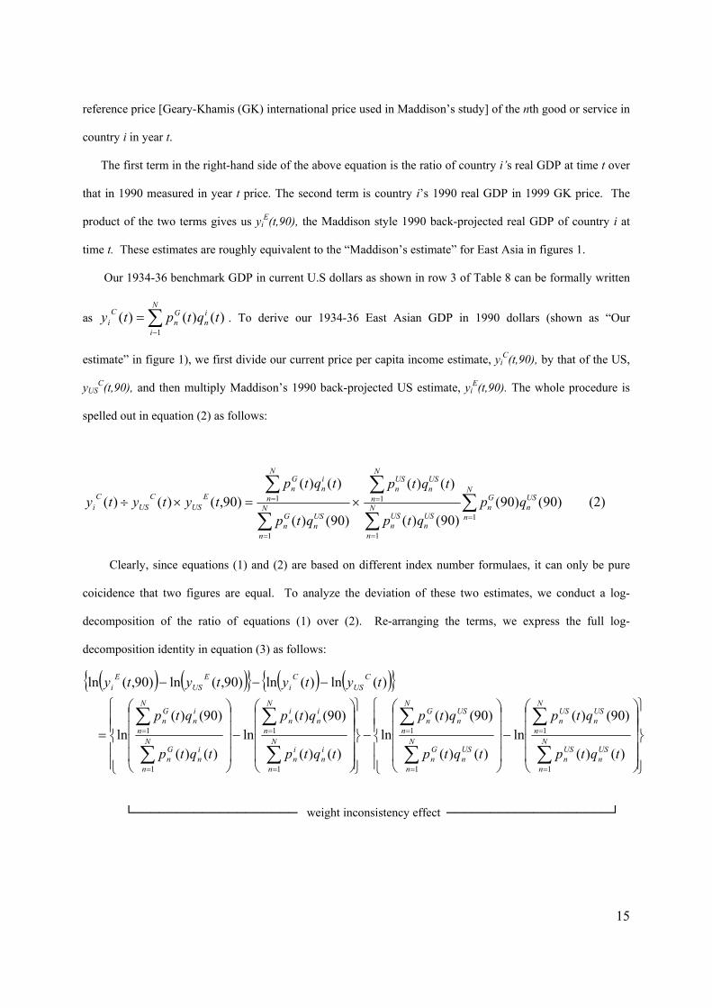
Our 1934-36 benchmark GDP in current U.S dollars as shown in row 3 of Table 8 can be formally written

as ∑−

=N

i

in

Gn

Ci tqtpty

1

)()()( . To derive our 1934-36 East Asian GDP in 1990 dollars (shown as “Our

estimate” in figure 1), we first divide our current price per capita income estimate, yiC(t,90), by that of the US,

yUSC(t,90), and then multiply Maddison’s 1990 back-projected US estimate, yi

E(t,90). The whole procedure is

spelled out in equation (2) as follows:

×=×÷

∑

∑

=

=N

n

USn

Gn

N

n

in

Gn

EUS

CUS

Ci

qtp

tqtptytyty

1

1

)90()(

)()()90,()()( ∑

∑

∑=

=

=N

n

USn

GnN

n

USn

USn

N

n

USn

USn

qpqtp

tqtp

1

1

1 )90()90()90()(

)()( (2)

Clearly, since equations (1) and (2) are based on different index number formulaes, it can only be pure

coicidence that two figures are equal. To analyze the deviation of these two estimates, we conduct a log-

decomposition of the ratio of equations (1) over (2). Re-arranging the terms, we express the full log-

decomposition identity in equation (3) as follows:

( ) ( ){ } ( ) ( ){ }

⎪⎪⎭

⎪⎪⎬

⎫

⎪⎪⎩

⎪⎪⎨

⎧

⎟⎟⎟⎟

⎠

⎞

⎜⎜⎜⎜

⎝

⎛

−⎟⎟⎟⎟

⎠

⎞

⎜⎜⎜⎜

⎝

⎛

−

⎪⎪⎭

⎪⎪⎬

⎫

⎪⎪⎩

⎪⎪⎨

⎧

⎟⎟⎟⎟

⎠

⎞

⎜⎜⎜⎜

⎝

⎛

−⎟⎟⎟⎟

⎠

⎞

⎜⎜⎜⎜

⎝

⎛

=

−−−

∑

∑

∑

∑

∑

∑

∑

∑

=

=

=

=

=

=

=

=N

n

USn

USn

N

n

USn

USn

N

n

USn

Gn

N

n

USn

Gn

N

n

in

in

N

n

in

in

N

n

in

Gn

N

n

in

Gn

CUS

Ci

EUS

Ei

tqtp

qtp

tqtp

qtp

tqtp

qtp

tqtp

qtp

tytytyty

1

1

1

1

1

1

1

1

)()(

)90()(ln

)()(

)90()(ln

)()(

)90()(ln

)()(

)90()(ln

)(ln)(ln)90,(ln)90,(ln

└─────────────────── weight inconsistency effect ───────────────────┘

16

⎟⎟⎟⎟

⎠

⎞

⎜⎜⎜⎜

⎝

⎛

−⎟⎟⎟⎟

⎠

⎞

⎜⎜⎜⎜

⎝

⎛

+

∑

∑

∑

∑

=

=

=

=N

n

USn

Gn

N

n

USn

Gn

N

n

in

Gn

N

n

in

Gn

qtp

qp

qtp

qp

1

1

1

1

)90()(

)90()90(ln

)90()(

)90()90(ln (3)

└────────terms of trade effect────────┘ Equation (3), as cumbersome as it appears, has nice interpretative properties: a positive (or negative)

value implies an over-estimate (or under-estimate) of the t period per capita income using the 1990 back-

projection method. We summarize the first four terms in equation 3 as “weight inconsistency” effect defined

earlier in Szilágyi (1984). The first two terms in this component are the log-difference between country i’s real

GDP growth rates from t to 1990 measured using the t period international price and that based on the t period

domestic price. The next two terms is this same log-difference but for the U.S, our reference country. Since

international price for the 1930s in our study is expressed as the average of US and country i’s price, the weight

inconsistency effect for the U.S is negligible. We can focus on the first two terms for country i.

In this case, the weight inconsistency effect stems from the divergence between international price and

domestic price in the t period. As partly shown in our matched price items for the mid-1930s, prices in East

Asia relative to the U.S tended to be relatively lower in the primary and service sectors but higher in

manufacturing and industrial goods. With rapid economic growth, structural transformation and increasing

integration of East Asian economies with the world economies during the post-War period, their domestic price

structure is converging to the world price structure with a rise in the share of manufacturing sectors and service

sectors at the expense of agricultural sectors. International price at time t assigns relatively lower price weights

than domestic price to the expanding manufacturing sector but higher price weights to the slow-growing

primary sector and expanding service sectors. Thus, whether or not real GDP growth rates measured using the

1930s international price would be higher or lower than those measured using the 1930s domestic price, or

whether or not backward extrapolation would under- or over-estimate past per-capita GDP of countries which

experienced rapid industrialization and globalization would depend on the relative magnitude of these mutually

offsetting forces.

Unfortunately, this theoretical issue is particularly difficult to test given the way that long-term real GDP

series are constructed using multiple benchmarks or chain-indexing, which, in fact, aims to mitigate this weight

inconsistency biases. Since the choice of benchmark periods or price deflators are rarely uniform for different

17

countries compared, it becomes hard to disentangle all these effects in order to test for either the direction or

magnitude of backward bias.

The second component is captured by the last two terms in Equation (3). The two terms are an index of

international GK price between t and 1990 for country i and US, each measured by the weight of their output

respectively at 1990. Independently, these two terms take a positive (or negative) value if international price

from year t to 1990 rises (or falls) for their output at 1990. With certain assumptions, this price index is

equivalent to a country’s Paasche terms of trade index. The log-difference between these two terms, defined as

the “terms of trade” effect, indicates if improvement (or deterioration) in country i’s Paasche terms of trade is

greater than that for the U.S, backward projection will over-estimate (or under-estimate) country i’s output at

time t. Intuitively, this can be understood by the following hypothetical example. Suppose there are two open

economies A and B. Country A is a producer of primary goods and country B is a producer of manufacturing

goods. Suppose two countries’ total GDP are equal measured at the international prices in 1930. By 1990,

both countries have doubled their output but international prices for primary goods have also doubled while

those for manufacturing goods have remained constant. This would imply country A’s GDP is twice that of

country B based on 1990 price due to the terms of trade improvement. If we project backward based on the

1990 international price, we will overestimate the relative standing between countries A and B in comparison to

that based on the 1930 international price.

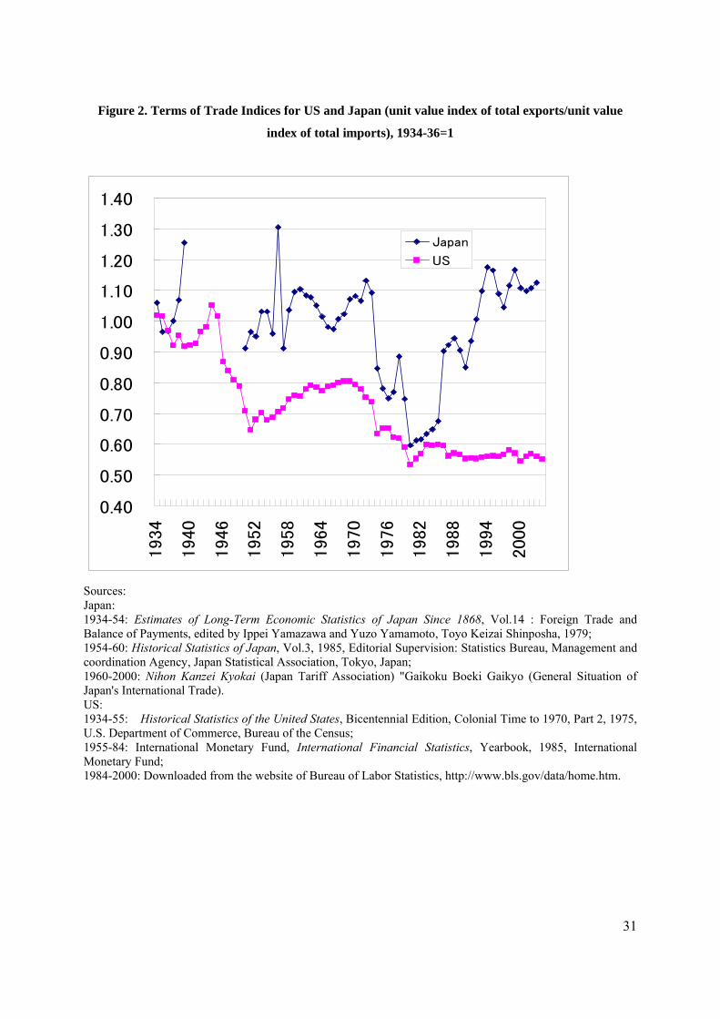
As regards the terms of trade (TOT) effect, we manage to gather some preliminary data for an empirical test.

Figure 2 presents our terms of trade indices for Japan and US linked from 1935 to 1990. It shows that the US

terms of trade deteriorated by 54 percent compared with that of Japan. This would imply, according to our

decomposition, an upward bias in the 1930s Japanese per capita income based on the 1990 back-projection, a

result consistent with our earlier empirical findings. In the Appendix, we develop an empirical test based on

the European Union data on an interval of 5 years in the several rounds of post-War ICP studies. There, we

show that the quantitative magnitude of this upward bias can be measured by a cross-term of terms of trade

change and trade dependency ratio. Since trade dependency ratio (the average of exports and imports over

GDP) was 10% for Japan and only 8% for US in 1990 respectively, the terms of trade improvement for Japan

18

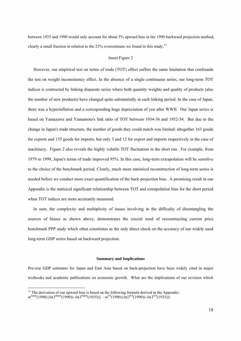
between 1935 and 1990 would only account for about 3% upward bias in the 1990 backward projection method,

clearly a small fraction in relation to the 23% overestimate we found in this study.13

Insert Figure 2

However, our empirical test on terms of trade (TOT) effect suffers the same limitation that confounds

the test on weight inconsistency effect. In the absence of a single continuous series, our long-term TOT

indices is contructed by linking disparate series where both quantity weights and quality of products (also

the number of new products) have changed quite substantially at each linking period. In the case of Japan,

there was a hyperinflation and a corresponding huge depreciation of yen after WWII. Our Japan series is

based on Yamazawa and Yamamoto's link ratio of TOT between 1934-36 and 1952-54. But due to the

change in Japan's trade structure, the number of goods they could match was limited: altogether 163 goods

for exports and 135 goods for imports, but only 3 and 12 for export and imports respectively in the case of

machinery. Figure 2 also reveals the highly volatile TOT fluctuation in the short run. For example, from

1979 to 1999, Japan's terms of trade improved 95%. In this case, long-term extrapolation will be sensitive

to the choice of the benchmark period. Clearly, much more statistical reconstruction of long-term series is

needed before we conduct more exact quantification of the back-projection bias. A promising result in our

Appendix is the statisical significant relationship between TOT and extrapolation bias for the short period

when TOT indices are more accurately measured.

In sum, the complexity and multiplicity of issues involving in the difficulty of disentangling the

sources of biases as shown above, demonstrates the crucial need of reconstructing current price

benchmark PPP study which often constitutes as the only direct check on the accuracy of our widely used

long-term GDP series based on backward projection.

Summary and Implications

Pre-war GDP estimates for Japan and East Asia based on back-projection have been widely cited in major

textbooks and academic publications on economic growth. What are the implications of our revision which

13 The derivation of our upward bias is based on the following formula derived in the Appendix: mJapan(1990){ln(TJapan(1990))–ln(TJapan(1935))} – mUS(1990){ln(TUS(1990))–ln(TUS(1935))}

19

reduces the per capita income estimate for the mid-1930s from 2,154 dollars to 1,745 dollars (in 1990 prices)?

If we compare this value with those for other countries in Maddison’s latest data set, it would be lower than

those of almost all other Western European countries, including Spain, Italy and Greece, only comparable to

USSR. Clearly, if possible, it is advisable to conduct similar pre-War PPP studies as carried out in a recent

preliminary study by Ward and Devereux (2005) to check the consistency of other back-projected estimates in

Maddison’s data set.

If we compare our estimate for Japan into Maddison’s data set for Asian countries, Japanese per capita

income would end up being only marginally higher that of Malaysia or the Philippines. Backward and forward

projection of our mid-1930s PPP adjusted income estimate sheds new light on Japan’s initial conditions in early

Meiji period. For example, projecting backward from the level of 1,745 dollars (in 1990 prices) in the mid-

1930s - rather than Maddison’s 2,154 dollars (in 1990 prices) – gives an 1880s Japanese per capita income of

about 600 dollars (in 1990 prices), only marginally higher than those in China and India but lower than in

Philippines and Thailand. In other words, on the eve of the first wave of industrialization in the 1880s, the

Japanese economy was near subsistence, no richer than those of its Asian neighbors, whom Japan was to

overtake or even colonize in the following few decades.

This is clearly quite a reassessment of prevailing view on both the initial conditions and the dynamics of

long-term economic growth for Japan and Asia in general. However, recent studies based on the comparison of

real wages seem to lend tentative support to this reassessment. For example, Bassino and Ma (2005) and Allen

et al. (2005) show that Japanese real wages in the 18th century were close to those in China and low-income

European countries such as Italy. Real wages only consistently rose above the Chinese level after the 1890s and

reached more than twice China’s level by the 1920s, a result consistent with the per capita GDP differences

indicated in this PPP study for the mid-1930s. Studies by Bassino and Eng (2002) and Bassino (2005) also

reveal that daily nominal wages for unskilled laborers and carpenters in Tokyo in 1935 were not much higher

than those in Bangkok, Singapore, or Penang in British Malaya. As consumer price levels, particularly food

prices, were much lower in those Southeast Asian cities, their studies suggest that real wages in Tokyo were

lower than in those cities.

=0.1*{ln(0.85) – ln(1)} – 0.08*{ln(0.55) – ln(1)}=0.032; where mi(t) and T i(t) denote coutrry i’s trade dependency ratio and terms of trade.

20

It is long recognized that pre-War economic growth in Japan was respectable but nothing nearly as

spectacular as in the high-growth era of the Post-War period. Considering the huge per-capita income gap

between Japan the world leaders in the late 19th century, pre-War Japanese economic growth is more of

keeping-up rather than catching-up. The pre-War catch-up (or even overtaking) seems to be more with the

resource rich Southeast Asia. Japan’s economic convergence with the world income leaders is truly a post-war

phenomenon. This is particularly striking if one compares the pre- and post-war income gaps within East Asia.

Income differentials of Japan, Taiwan, Korea versus China in the 1980s were multiples of those in the 1930s.

In this regard, China’s rapid economic growth since the 1980s, particularly in some of her coastal regions, is

partly a making-up for her missed opportunities.

Of course, the big question is: why was it Japan - rather than Malaysia or Thailand – that caught up so

quickly in the post-War period despite their possibly common starting points? We can provide some

conjectures. Bassino (2005)’s wage data shows that the skill premium for carpenters vis-à-vis unskilled

laborers in Tokyo was smaller than in any of the Southeast Asian cities, indicating the existence of a large pool

of skilled workers in Japan in comparison with Southeast Asia. A recent study by Godo and Hayami (2003)

reveal that in the 1930s, average years of schooling in Japan were already over 60% of the U.S. level despite

the much greater lag in per capita income. Japan then already had some of the world’s most dynamic industries,

a sizable entrepreneurial class, a competent bureaucracy and, of course, a nation state. Was Japan already on a

course of convergence in the pre-war era but was thrown off course by the war? This PPP study provides new

answers and raises new questions.

In sum, our study provides a set of pre-war benchmark PPP converters that allow us to carry out

comparisons of income, consumption, and other monetary indicators for East Asia in a global context. Our pre-

war PPP converters confirm that market exchange rate conversion consistently under-estimated per capita

incomes of East Asia. Our PPP results also reveal biases associated with the 1990 backward projection method.

Our preliminary theoretical and empirical analysis pointed out the direction of such bias and set out a

framework for future research which will enable us to quantify the magnitude of this bias and to eventually

“consistentize” our new levels with growth trend in the long-term GDP series for East Asia and beyond.

21

Our finding that Japanese per capita income in the mid-1930s or the entire pre-war period was much

lower than widely believed is a major revision of our existing interpretation of long-term economic growth in

Japan and East Asia. It may also have further reverberations on our interpretation of the determinants of long-

term economic growth. The fact that that Japan, or East Asia in general, were historically very poor, may even

a message of blessing for developing countries today: initial poverty itself is no curse to a nation’s aspirations

for prosperity.

References

Allen, Bob, Jean-Pascal Bassino, Debin Ma, Christine Moll-Murata, and Jan Luiten van Zanden (2005) “Wages,

Prices and Living Standards in China, Japan and Europe” downloadable at http://gpih.ucdavis.edu/Papers.htm.

Balassa, Bela (1964) “The Purchasing Power Parity Doctrine: A Reappraisal,” Journal of Political Economy,

vol. 72, pp. 584-596. Bassino, Jean-Pascal, and Pierre van der Eng (2002) “Economic Divergence in East Asia: New Benchmark

Estimates of Levels of Wages and GDP, 1913-1970,” paper presented at the XIII Economic History Congress, July 22-26, 2002, Buenos Aires.

Bassino, Jean-Pascal, and Debin Ma (2005) “Japanese Wages for Unskilled Laborers in 1730-1910: an

International Perspective,” forthcoming in Research in Economic History. Bassino, Jean-Pascal (2005) “How Poor Was Asia before the Industrialization?” unpublished manuscript,

Tokyo: Maison Franco-Japonaise. Bureau of the Census (1939), Census of Manufactures, 1939, Washington D.C.: Bureau of the Census. Clark, Conlin (1940, 1957) Conditions of Economic Progress, London: St. Martins’s Press. Emi, Koichi and Shionoya, Yuichi (1966) Estimates of Long-Term Economic Statistics of Japan since 1868

(LTES) vol. 7, Government Expenditure, Tokyo: Toyo Keizai Shinposha. Emi, Koichi (1971) Estimates of Long-Term Economic Statistics of Japan since 1868 (LTES) vol. 4, Capital

Formation. Tokyo: Toyo Keizai Shinposha. Fukao, K., Ma, D., and Yuan, T. (2006) “International Comparison in Historical Perspective: Reconstructing

the 1934-36 Benchmark Purchasing Power Parity for Japan, Korea and Taiwan,” Discussion Paper Series A, no. 442, Tokyo: the Institute of Economic Research, Hitotsubashi University, forthcoming in Explorations in Economic History.

Godo, Yoshihisa, and Yujiro Hayami (2002) “Catching Up in Education in the Economic Catch-up of Japan

with the United States, 1890 1990” Economic Development and Cultural Change, vol. 50, no. 4, pp. 961-78.

22

Heston, Alan and Robert Summers (1993) “What Can Be Learned from Successive ICP Benchmark Estimates?” A. Szirmai, B. Van Ark, and D. Pilat eds. Explaining Economic Growth, Amsterdam: North Holland.

Kravis, Irving B., Alan Heston, and Robert Summers (1975) A System of International Comparisons of Gross

Product and Purchasing Power, Baltimore: Johns Hopkins University Press. Kravis, Irving B., Alan Heston, and Robert Summers (1978) International Comparisons of Real Product and

Purchasing Power, Baltimore: Johns Hopkins University Press. Kravis, Irving B., Alan Heston, and Robert Summers (1982) World Product and Income, International

Comparisons of Real Gross Product,. Baltimore: Johns Hopkins University Press. Liu, Ta-chung (1946) China’s National Income 1931-36, An Exploratory Study, Washington, D.C.: the

Brookings Institution. Liu, Ta-chung, and Kung-chia Yeh (1965) The Economy of the Chinese Mainland: National Income and

Economic Development, 1933-1959, Princeton, New Jersey, Princeton University Press, 1965. Maddison, Angus (1995) Monitoring the World Economy 1820-1992, Paris, France: OECD. _______________(1998) Chinese Economic Performance in the Long Run, Paris, France: OECD. _______________ (2001) The World Economy: a Millennial Perspective, Paris, France: OECD. _______________ (2003) The World Economy: Historical Statistics, Paris, France: OECD. Minami, Ryoshin (1965). Railroads And Electric Utilities. Kazushi Ohkawa and others eds. Estimates of Long-

Term Economic Statistics of Japan since 1868 (LTES) vol. 12. Tokyo: Toyo Keizai Shinposha. Ministry of Commerce and Industry, Statistics Department, Japanese Government (1938) Koujyou Toukei

(Factory Statistics) 1938. Mizoguchi, Toshiyuki (1975) Taiwan, Chosen no Keizai Seicho: Bukka Tokei wo Chushin to shite (Economic

Growth of Taiwan and Korea: a Study of Prices). Tokyo: Iwanami Shoten. Mizoguchi, Toshiyuki, and Umemura, Mataji, eds. (1988), Kyu Nihon Shokuminchi Keizai Tokei: Suikei to

Bunseki (Basic Economic Statistics of Former Japanese Colonies 1895-1938), Tokyo: Toyo Keizai Shinposha.

Mizoguchi, Toshiyuki, and Nojima, Noriyuki (1993) “194-55 Nen ni Okeru Kokumin Keizai Keisan no Ginmi

(Nominal and Real GDP of Japan: 1940-55),” Nippon Tokei Gakkaishi (Journal of the Japan Statistical Society). Vol. 23, No. 1, pp. 91-107.

Mizoguchi, Toshiyuki, and Nojima, Noriyuki (1996) “Taiwan, Kankoku no Kokumin Keizai Keisan Choki

Keiretsu no Suikei” (Estimation of the Long Term National Accounts of Taiwan and Korea) Asian Historical Economic Statistics Project Discussion Paper: R96-6, Tokyo: Institute of Economic Research, Hitotsubashi University.

OECD, Department of Economics and Statistics, OECD (1976) National Accounts of OECD Countries, OECD. OECD, Department of Economics and Statistics, OECD (1999) National Accounts of OECD Countries, OECD. Keizai Kikaku-cho (Economic Planning Agency), Japanese Government (1963) Showa 37 Nendo Kokumin

Shotoku Hakusho (White Paper on National Income 1962 C.Y.), Tokyo: Printing Office, Ministry of Finance.

23

Keizai Shingi-cho (Economic Counsel Board) Japanese Government (1953) Showa 27 Rekinen Kokumin

Shotoku Hokoku（Report on National Income Statistics 1952 C.Y.） , Tokyo: Keizai Shingi-cho (Economic Counsel Board).

Keizai Shingi-cho, Chosabu Tokeika (Stiatistical Division, Economic Counsel Board) Japanese Government

(1953) Senzen Kijun Shohi Suijun—Tokyo SanSyutsu Hoho１ Tukei Siryo No.78.（Pre-War Standard Consumption Level – Method of Calculation for Tokyo (1), Statistical Materials No. 78）, Tokyo: Keizai Shingi-cho (Economic Counsel Board).

Ohkawa, Kiyoshi, and Shinohara Miyohei (1979) Patterns of Japanese Development: A Quantitative Appraisal,

New Haven, CT.: Yale University Press. Ou, Baosan, ed. (1947) Zhongguo Guomin Soude (National Income of China), vols. 1 and 2, Shanghai:

Zhonghua sujui. Perkins, Dwight H. (1975) “Growth and Changing Structure of China’s Twentieth-Century Economy,” in

Dwight H. Perkins, ed., China’s Modern Economy in Historical Perspective. Stanford: Stanford University Press.

Pilat, Dirk (1994) The Economics of Rapid Growth: The Experience of Japan and Korea, Aldershot UK and

Brookfield US: Edward Elgar. Samuelson, Paul (1964) “Theoretical Notes on Trade Problems,” Review of Economics and Statistics, vol. 46:

pp. 145-154. Szilagyi, Gyorgy (1984) “Updating Procedures of International Comparisons Results” Review of Income and

Wealth, vol. 30, pp. 153-65. Summers, Robert, and Alan Heston (1991) “The Penn World Table (Mark 5): An Expanded Set of International

Comparisons, 1950-88,”Quarterly Journal of Economics, vol. 106, no. 2, pp. 327-68. U.S. Department of Labor, Bureau of Labor Statistics, Department of Agriculture. Bureau of Home Economics

Micro data of Study of Consumer Purchases in the United States, 1935-1936, ICPSR 8908, http://www.icpsr.umich.edu/.

U.S. Department of Labor, Bureau of Labor Statistics (1938) “Retail Prices of Food 1923-36,” Bulletin, no. 635.

Washington D.C.: Bureau of Labor Statistics. ___________________________________________ (1941) “Changes in Cost of Living in Large Cities in the

United States, 1914-41,” Bulletin, no. 699, Washington D.C.: Bureau of Labor Statistics. ___________________________________________ (1941) Handbook of Labor Statistics Bulletin No. 694,

vols. I and II. Washington D.C.: Bureau of Labor Statistics. U.S. Department of Commerce, Bureau of the Census (1975) Historical Statistics of the United States, Parts 1

and 2 (Bicentennial Edition), Washington D.C.: Bureau of the Census. ____________________________________________ (1939) Statistical Abstract of the United States 1938,

Washington D.C.: Government Printing Office. U.S. Department of Commerce, Bureau of Economic Analysis (1998), “GDP AND OTHER MAJOR

NIPA SERIES, 1929-97” Survey of Current Business, Aug 98, Vol. 78, Issue 8. Yamamoto, Yuzou (2000), Nihon Shokuminchi Keizai Shi Kenkyu (Studies on the Economic History of

Japanese Colonies), Nagoya: Nagoya University Publishing House.

24

Yuan Tangjun and Kyoji Fukao (2002) “1930 Nendai Niokeru Nippon, Chosen, Taiwan Kanno Kobairyoku

Heika: Jissitsu Shohi Suijun no Kokusai Hikaku (The Purchasing Power Parity of Japan, Korea and Taiwan in the 1930s: An International Comparison of Real Consumption),” Keizai Kenkyu (the Economic Review), vol.53, no. 3, pp. 322-336.

Yuan Tangjun (2005) “Cyugoku no Keizai Hatten no Shoki Jokyo: 1930 Nendai Niokeru Jissitsu Shohi Suijun

no Kokusai Hikaku (The Initial Condition of China’s Economic Growth: An International Comparison of Per Capita Real Consumption Level in the 1930s),” Chapter 1 in T. Yuan, Chugoku no Keizai Hatten to Bumonkan Shigen Haibun (China’s Economic Growth and the Resource Reallocation among Sectors), Ph.D. Dissertation, Graduate School of Economics, Hitotsubashi University.

Wang, Qingyi (1988) Zhongguo Nenyuan (Chinese Energy). Beijing: China Metallic Industry Press. Ward, Marianne, and John Devereux (2003) “Measuring British Decline: Direct Versus Long-Span Income

Measures.” Journal of Economic History. Vol. 63, no. 3, 826-51. Ward, Marianne, and John Devereux (2005) “International Comparisons of Incomes, Labor Productivity and

Capital Stocks for Developed Economies: 1870-1950,” paper presented at UC Davis workshop, Estimating Production and Income Across Nations and over Time, May 31-June 1, 2005, Davis, CA: UC Davis, Institute of Governmental Affairs.

Watanabe, Tsunehiko, and Komiya, Ryutaro (1958) “Findings from Price Comparisons Principally Japan vs.

the United States” Zeitschrift des Instituts für Weltwirtschaft an der Universität Kiel, vol. 81, no. 1, pp. 81-96.

25

Table 1. Consumption Price Levels of China Relative to Japan (1934-36 Japan =1)

Chinese expenditure

weight

Japanese expenditure

weight

Fisher average

Total 0.65 0.86 0.75

Food 0.66 0.78 0.72

Lighting and heat 0.41 1.36 0.75

Clothing and bedding 0.86 0.93 0.89

Housing expenses 0.70 0.57 0.63

Miscellaneous 0.81 0.99 0.90

Source: See text.

Table 2. Consumption Price Levels of Japan Relative to the U.S (1934-36 U.S =1)

Japanese expenditure

weight

U.S. expenditure

weight

Fisher average

Total 0.35 0.61 0.46 Food 0.38 0.64 0.50

Lighting and heat 1.09 0.91 1.00 Clothing and bedding 0.25 0.51 0.36

Housing expenses 0.59 0.69 0.63 Miscellaneous 0.28 0.50 0.37

Source: See text.

26

Table 3. Consumption Price Levels of East Asian Countries Relative to the U.S. (Fisher Average)

1934-36 U.S. =1

China Taiwan Korea Japan

Total 0.34 0.39 0.44 0.46

Food 0.35 0.43 0.46 0.49 Lighting and heat 0.75 0.79 0.82 1.00

Clothing and bedding

0.32 0.34 0.34 0.36

Housing expenses 0.40 0.46 0.56 0.63 Miscellaneous 0.33 0.30 0.26 0.37

Tradable* 0.79 0.88 0.93 0.57 Non-tradable* 0.71 0.78 0.71 0.40

*Relative price levels for tradable and non-tradable for Japan are calculated relative to the U.S. The rest three economies are computed relative to Japan. Notes:

1. Tradable goods for Korea and Taiwan can be found in Fukao, Ma and Yuan (2006). 2. Tradable goods for China: food, clothing and bedding, firewood, coal, matches, lamp oil, wooden boards,

wash basins, hygiene products, soap, toothbrushes, medical alcohol. 3. Tradable goods for Japan are items marked with “1” in Appendix Table II. 4. For the Japan-China comparison, the weights used for tradables are 63 percent for Japan and 89 percent for

China. For the Japan-U.S. comparison, the weights used for tradables are 47 percent for Japan and 42 percent for the U.S.

Table 4. Aggregate Consumption Expenditure Weights for 1934-36

China Taiwan Korea Japan U.S.

Food 68.65 47.99 65.82 41.3 33.2 Lighting and heat 8.32 5.84 9.75 4.8 5.8

Clothing and bedding 8.48 6.87 7.15 10.6 13.3

Housing expenses 5.29 7.67 5.57 10.2 21.0

Miscellaneous 9.25 31.63 11.71 32.2 26.7

Sources: For details on the weights and data sources for Japan, Taiwan, and Korea, see Fukao, Ma, and Yuan (2006). The weights for China are largely based on Zhang Donggan (2001, p.375-6). The rural share of the population in Taiwan and Korea are 52 and 75 per cent, respectively, based on data from Mizoguchi and Umemura (1988), pp. 235, 237, 263 and 268.

27

Table 5. Relative Price Levels for Private Investment for Japan and the U.S in 1935

Japan U.S. Japan/U.S. Japaneseweight

U.S.weight

Fisheraverage

Equipment (Machinery and equipment) 0.5 0.5 0.88 0.88 0.88 0.88Construction 0.24 0.51 0.35

Cement 0.0625 0.075 0.68Pig iron 0.0625 0.075 0.78Nails 0.0625 0.075 0.72Tin plate 0.0625 0.075 0.87Wages 0.25 0.2 0.14

1.0 1.0 0.68 0.38 0.70 0.51

Weight

Total

Japanese price level (U.S.=1)

Sources: 1. The Japan/U.S. relative price for equipment (metals and machinery) is from Pilat (1994), Table 2.5, p. 27.

construction wages are from Appendix Table II. Relative prices for the rest are from wholesale price statistics of both U.S. and Japan.

2. The weights for Japanese equipment and construction investment are based on Emi (1971), p. 10; for the U.S. the weights are based on Historical Statistics, Part I, p. 283 for 1947. The shares of raw materials and labor for construction investment for U.S. are from Historical Statistics, Part I, p. 282; for Japan, they are from Fukao, Ma, and Yuan (2006).

28

Table 6. Relative Price Levels for Government Expenditure for Japan and the U.S. in 1935

Japan U.S. Japan/U.S. Japaneseweight

U.S.weight

Fisheraverage

Labor costs 0.24 0.45 0.07 0.07 0.07 0.07Material costs 0.57 0.63 0.60

Food 0.03 0.02 0.53Textiles 0.03 0.01 0.51Wood products 0.03 0.06 0.40Medical costs 0.14 0.06 0.37Chemical Products 0.11 0.09 1.33Metals & machinery 0.06 0.02 0.88Construction 0.08 0.24 0.48Transportation and communication 0.21 0.04 0.54Coal 0.02 0.01 0.89

Electricity 0.05 0.01 0.96Total 1.01 1.00 0.23 0.38 0.30

Weights Japanese price level (U.S.=1)

Sources: 1. Labor costs for Japan are based on the salaries of government employees taken from Emi and Shionoya (1966),

pp. 222-3. Labor costs for U.S. are from Historical Statistics, Part II, pp. 1100-1. Data on chemical products, metals & machinery, transportation and communication are from Pilat (1994), p. 24. The remaining figures are from Appendix Table II.

2. The weight for labor and material costs for Japan is based on Emi and Shionoya (1966), pp.31-2; the equivalent weight for the U.S. is based on Historical Statistics, pp. 282-3. (The share of material costs is assumed to be equal to the share of total intermediate inputs in government purchases, while value added is assumed to be equal to labor costs. The U.S. shares used are for the 1950s and 60s). The weights for materials for Japan are based on Fukao, Ma, and Yuan (2006), Table 5. The weights for materials for the U.S. are based on Historical Statistics, pp. 282-3.

Table 7. East Asian Price Levels Relative to the U.S. (1934-36)

Source Note: In the case of Taiwan and Korea, the relative price level for each expenditure category (the five consumption categories, private investment, and government expenditure) is calculated multiplying the Fisher average price level of these countries relative to Japan by the Fisher average price level of Japan relative to the U.S. The price levels for the total GDP of Taiwan, Korea and Japan relative to the U.S. are calculated as Fisher averages based on each country’s expenditure weights and U.S. expenditure weights for the five consumption categories, private investment and government expenditure. Price levels and weights for Korea and Taiwan are based on Fukao, Ma, and Yuan (2006). US weights are based on U.S. Department of Commerce (1998), “GDP AND OTHER MAJOR NIPA SERIES, 1929-97” Survey of Current Business, Aug 1998, p.147.

Taiwan Korea Japan U.S. Taiwan Korea Japan

Consumption 0.73 0.84 0.70 0.77 0.40 0.44 0.46

Private investment 0.20 0.11 0.18 0.08 0.48 0.50 0.51

Government expenditure 0.07 0.05 0.12 0.15 0.26 0.27 0.30

GDP 1.00 1.00 1.00 1.00 0.39 0.44 0.44

Expenditure weight Price level (Fisher average, U.S.=1)

29

Table 8. 1934-36 East Asian Per Capita GDPs in 1934-36 U.S. Dollars and Relative to the U.S. U.S. Japan Taiwan Korea China 1. Exchange rate converted estimate 574.7 79.4

(14%) 50.7 (9%)

29.9 (5.2%)

20.7 (3.6%)

2. Relative GDP price levels 1 0.44 0.39 0.44 0.37

3. PPP adjusted estimate = 1÷2

574.7 179.2 (31%)

130 (23%)

68 (12%)

55.8 (10%)

Sources: 1. GDP for China from Liu and Yeh, p. 68, Table 10; for Japan from Ohkawa and Shinohara (1979), for Taiwan

and Korea from Mizoguchi and Umemura (1988); for the U.S. from the Historical Statistics of the U.S. (the Bicentennial Edition, 1975).

2. 1934-36 exchanges rates: 1 U.S. dollar = 3.33 yen, 1 Chinese yuan = 1.1 yen. Table 9. Relative GDP Price Levels and Relative GDP per capita (U.S. = 100) Relative GDP price

levels Relative GDP per capita Sources

1934-36 44 31 This study 1939 60.7* 27 Pilat 1994, p.24. 1952 52** 18 Watanabe and Komiya 1958 1970 68 59 Kravis et al. 1982, p.13 & 21 1973 95 64 Kravis et al. 1982, p.13 & 21 1975 90 68 Kravis et al. 1982, p.13 & 21

* The Watanabe and Komiya study did not calculate relative per capita GDP for 1952. We recalculate it with the exchange rate at 1 U.S. dollar = 360 yen and the 52% relative price levels. The per capita GDP estimates for Japan and the U.S. in 1938 and 1952 current prices are from Ohkawa and Shinohara (1979, p.283) and Historical Statistics of the United States (1975, p. F10-30).

30

Figure 1. Comparison of Our Current Price PPP Per Capita GDP with Maddison’s Back-Projected Estimate (in 1990 U.S. Dollars)

543662

1266

1745

2154

562

12241212

0

500

1000

1500

2000

2500

Japan Taiwan Korea China

1990 U

.S. D

ollars

Our estimate

Maddison's estimate

31

Figure 2. Terms of Trade Indices for US and Japan (unit value index of total exports/unit value

index of total imports), 1934-36=1

0.40

0.50

0.60

0.70

0.80

0.90

1.00

1.10

1.20

1.30

1.40

1934

1940

1946

1952

1958

1964

1970

1976

1982

1988

1994

2000

Japan

US

Sources: Japan: 1934-54: Estimates of Long-Term Economic Statistics of Japan Since 1868, Vol.14 : Foreign Trade and Balance of Payments, edited by Ippei Yamazawa and Yuzo Yamamoto, Toyo Keizai Shinposha, 1979; 1954-60: Historical Statistics of Japan, Vol.3, 1985, Editorial Supervision: Statistics Bureau, Management and coordination Agency, Japan Statistical Association, Tokyo, Japan; 1960-2000: Nihon Kanzei Kyokai (Japan Tariff Association) "Gaikoku Boeki Gaikyo (General Situation of Japan's International Trade). US: 1934-55: Historical Statistics of the United States, Bicentennial Edition, Colonial Time to 1970, Part 2, 1975, U.S. Department of Commerce, Bureau of the Census; 1955-84: International Monetary Fund, International Financial Statistics, Yearbook, 1985, International Monetary Fund; 1984-2000: Downloaded from the website of Bureau of Labor Statistics, http://www.bls.gov/data/home.htm.

32

U M L U M L Japan China China/Japan. in PPP

Chineseweight

Japanese weight

Fisheraverage

Total Exchange rate Yen Yuan Yuan/Yen 1Yen=0.88Yuan 0.65 0.86 0.75

Food 68.7 40.9 0.66 0.78 0.72Grain 68.5 100.0 35.3 100.0 0.69 0.68 0.68

Rice 69.9 93.3 1 kg 0.24 0.14 0.59 0.67Wheat 30.1 6.7 1 kg 0.21 0.13 0.63 0.72

Vegetables 8.8 100.0 8.9 100.0 0.70 0.77 0.74Soybeans 1.7 13.9 1 kg 0.23 0.11 0.45 0.52Other beans 7.3 9.8 1 kg 0.19 0.06 0.35 0.40Potatoes 5.9 2.9 1 kg 0.07 0.03 0.38 0.43Cabbages 63.0 43.7 1 kg 0.08 0.06 0.66 0.76

2.3 9.9 1 kg 0.08 0.03 0.39 0.44Fresh vegetables 9.0 9.9 10 monme (37.5 0.18 0.12 0.66 0.75Apples 0.1 2.5 100 monme (375 0.15 0.30 1.99 2.26Oranges 0.3 2.5 100 monme (375 0.08 0.14 1.78 2.03Bananas 0.1 2.5 1 kg 0.20 0.40 2.03 2.32Other fruits 10.1 2.5 100 monme (375 0.1 0.14 1.37 1.57

Ingredients 7.4 100.0 8.5 100.0 1.00 1.32 1.15Soysauce 18.0 27.0 1 litter 0.27 0.47 1.74 1.98Miso 8.0 17.7 1 kg 0.22 0.18 0.82 0.94Sugar 11.6 11.5 1 kg 0.40 0.62 1.57 1.79Salt 8.3 3.5 1 kg 0.07 0.20 2.79 3.18Oil 54.2 40.4 1 litter 1.03 0.67 0.65 0.74

Meat and Fish 5.9 100.0 13.5 100.0 0.37 0.82 0.55Pork 38.1 5.3 100 g 0.14 0.04 0.32 0.36Beef 27.0 12.8 100 g 0.16 0.04 0.23 0.26Chicken 2.5 2.0 100 g 0.21 0.07 0.34 0.39Fresh fish 14.9 20.5 1 kg 0.71 0.44 0.62 0.70Salty fish 3.8 20.5 1 kg 1.15 1.85 1.62 1.84Other seafood 6.3 20.5 1 kg 0.75 0.20 0.26 0.30Eggs 5.9 14.3 1 kg 0.62 0.37 0.59 0.68Milk 1.4 4.3 1 bottle 0.37 0.62 1.67 1.90

Others 1.0 100.0 23.8 100.0 0.77 0.81 0.79Sweets 11.7 25.0 1 kg 0.16 0.12 0.76 0.87Preserved vegetables 21.6 25.0 1 kg 0.16 0.12 0.76 0.87Tofu 25.1 25.0 1 cake 0.07 0.03 0.45 0.52Other processed food 41.6 25.0 100 monme (375 0.07 0.06 0.86 0.98

Drinks and 8.4 100.0 9.9 100.0 0.60 0.72 0.65Tobacco 51.4 39.1 1 package 0.15 0.16 1.06 1.21Alcohol 20.9 48.7 1 litter 0.85 0.15 0.18 0.21Tea 27.7 12.1 100 g 0.19 0.19 1.03 1.17

Lighting and 8.3 4.8 0.41 1.36 0.75Electricity 0.3 100.0 47.6 100.0 １kwh 0.14 0.17 1.26 1.87 1.87 1.87 1.87Fuel 97.0 100.0 48.9 100.0 0.40 0.90 0.60

Coal 6.0 11.8 10 kg 0.27 0.22 0.83 0.94Firewood 77.0 38.8 10 kg 0.26 0.08 0.30 0.35Charcoal 1.7 40.8 10 kg 0.81 1.00 1.24 1.41Lamp oil 15.3 8.6 1 kg 0.26 0.28 1.09 0.88

Others Matches 2.7 100.0 3.5 100.0 1packet 0.06 0.05 0.82 0.94 0.94 0.94 0.94Clothing and 8.5 10.7 0.86 0.93 0.89Clothing 80.3 100.0 72.8 100.0 0.85 0.95 0.90

Bleached cotton 79.4 49.8 1 roll 0.59 1.84 3.12 0.83White men's shirt 11.3 49.8 1 piece 2.13 2.00 0.94 1.07Cotton 9.2 0.5 1 kg 0.98 0.71 0.72 0.83

Personal items 19.7 100.0 27.2 100.0 0.90 1.42 1.13Sports shoes 50.0 69.7 1 pair 0.70 1.09 1.56 1.78Umbrella 50.0 30.3 1 piece 0.89 0.47 0.53 0.60

Housing 5.3 10.7 0.70 0.57 0.63Rent 61.6 100.0 97.3 100.0 0.55 0.55 0.55

Monthly housing rent 50.0 50.0 1 room (7.43 sq. 5.09 2.40 0.47 0.54Carpenter's wage 50.0 50.0 daily 1.97 0.96 0.49 0.55

Furniture 38.4 100.0 2.7 100.0 1.29 1.39 1.34Wooden board 50.0 50.0 3.3 sq. m. 1.98 1.77 0.89 1.02Wash basin 50.0 50.0 1 piece 0.31 0.49 1.56 1.77

Miscellaneous 9.2 32.9 0.81 0.99 0.90Trans. Rickshaw pullers' 4.9 100.0 6.2 100.0 daily 2.67 0.54 0.20 0.23 0.23 0.23 0.23Education 1.5 100.0 5.8 0.69 0.63 0.66

Teachers' wage 100.0 100.0 monthly 65.91 40.00 0.61 0.69Hygience 9.9 100.0 10.4 100.0 2.22 2.36 2.29

Soap 50.0 50.0 1 piece 0.09 0.24 2.57 2.93Toothbrush (Tokyo) 50.0 50.0 1 piece 0.15 0.23 1.56 1.78

Medicine Alcohol 5.8 100.0 12.8 100.0 1 bottle 0.83 0.73 0.88 1.00 1.00 1.00 1.00Entertainment Movie 19.2 100.0 21.3 100.0 once 0.30 0.20 0.67 0.76 0.76 0.76 0.76Other Newspapers 58.7 100.0 43.5 100.0 1 set 0.05 0.04 0.80 0.91 0.91 0.91 0.91Source: Yuan (2005).

Vegetables and fruits

Appendix Table I.　Chinese Price Level Relative to Japan (1934-36: Japan=1)

PriceUnit

Chinese price levelItems

Chinese weight Japanese weight Ratio toexchange

rates

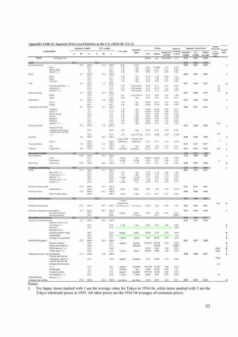
33

Notes: 1. For Japan, items marked with 1 are the average value for Tokyo in 1934-36, while items marked with 2 are the

Tokyo wholesale prices in 1935. All other prices are the 1934-36 averages of consumer prices.

Total Exchange rate dollars yen Yen/dollar 3.33 0.35 0.61 0.46

Food 41.3 33.2 0.38 0.64 0.50 Grain and bread 39.7 100.0 12.0 100.0 Unit Unit 0.40 0.61 0.49 1

Rice 92.9 3.1 1 lb 1 kg 0.08 0.2380 1.30 0.39 Wheat flour 5.8 16.7 1 lb 1 kg 0.05 0.23 2.11 0.64 Bread 1 , a 1.2 80.6 1 lb 1 lb 0.08 0.17 2.05 0.62

Meat 2.7 100.0 19.8 100.0 0.94 0.97 0.95 1Beef 63.9 51.7 1 lb 1 kg 0.14 1.28 4.04 1.21 Pork 26.8 34.1 1 lb 1 kg 0.32 1.40 2.01 0.60 Chicken 9.4 14.2 1 lb 1 kg 0.29 2.08 3.21 0.96

Fish 8.3 100.0 1.3 100.0 0.27 0.26 0.27 0Flounder/Halibut 1 , a 54.4 52.3 1 lb 100 monme 0.24 0.15 0.77 0.23 43Mackerel a 43.0 16.5 1 lb 100 monme 0.12 0.113 1.19 0.36 24Salmon 1 , a 2.5 31.1 1 lb 100 monme 0.24 0.17 0.85 0.25 24

Milk and Eggs 2.5 100.0 18.9 100.0 0.37 0.89 0.57 0Milk 23.0 77.6 1 qt. 1 go (180cc) 0.12 0.08 3.52 1.06 Eggs 77.0 22.4 1 doz 1 kg 0.36 0.62 1.03 0.31

Ingredients 8.5 100.0 3.0 100.0 0.75 0.84 0.79 1Salt a 10.3 10.3 1 lb 1 kg 0.053 0.117 1.01 0.30 Sugar 89.7 89.7 1 lb 1 kg 0.056 0.370 3.00 0.90

Vegetables and fruits 9.2 100.0 12.7 100.0 0.30 0.37 0.33 1Cabbage 6.7 7.2 1 lb 1 kg 0.040 0.080 0.90 0.27 Onion 1 5.4 11.3 1 lb 1 kg 0.044 0.104 1.06 0.32 Sweet potato 20.4 4.1 1 lb 1 kg 0.04 0.08 0.87 0.26 Potato 18.5 33.0 1 lb 1 kg 0.02 0.08 1.47 0.44 Spinach 12.1 8.2 1 lb 1 kan 0.076 0.30 0.48 0.14 Bananas 18.5 14.4 1 lb 1 kg 0.06 0.20 1.41 0.42 Apples 1 , a 18.5 21.6 1 lb 1 kg 0.054 0.15 1.26 0.38 545

Processed food 19.1 100.0 7.0 100.0 0.35 0.36 0.36 1Peanut oil and vegetable shortening 50.0 50.0 1 lb 1 kg 0.20 0.62 1.38 0.42 Canned pink salmon 1 , a 50.0 50.0 1 lb 1 can (235 g) 0.151 0.080 1.027 0.308 120

Alcohol 4.8 100.0 14.5 100.0 0.49 0.49 0.49 1

Beer a 100.0 100.0 1 quart (946 milliliters)

１bottle (720 milliliters) 0.27 0.33 1.63 0.49 3

Tea and drinks 1.2 100.0 2.6 100.0 0.37 0.37 0.37 1Tea 100.0 100.0 1 lb 1 kg 0.68 1.86 1.24 0.37

Tobacco Cigarettes a 3.9 100.0 8.1 100.0 1 package 1 package 0.135 0.15 1.11 0.33 0.33 0.33 0.33 704 1

Household Utilities 4.8 5.8 1.09 0.91 1.00 Fuel expenses 52.4 100.0 75.6 100.0 1.24 0.90 1.06 1

Coal 12.9 97.1 10 Kg 1 kg 0.0042 0.0272 2.96 0.89 Firewood a 87.1 2.9 10 Kg 10 Kg 0.06 0.27 4.40 1.32 6

Electricity Electricity 47.6 100.0 24.4 100.0 1 kwh 1 kwh 0.05 0.16 3.20 0.96 0.96 0.96 0.96 0

10.6 13.3 0.25 0.51 0.36 1Cloth 33.3 100.0 33.3 100.0 0.67 0.75 0.71

Raw silk 2 , b 20.0 20.0 1 lb 1 kg 1.50 11.23 3.40 1.02 Cotton yarn 2 , b 20.0 20.0 1 lb 1 kg 0.30 1.19 1.78 0.53 Muslin 2 , b 20.0 20.0 1 yard 1 yard 0.15 0.49 3.22 0.97 Woolen yarn 2 , b 20.0 20.0 1 lb 500 g 1.64 2.71 1.48 0.45 Serge 2 , b 20.0 20.0 1 yard I m 1.075 3.01 2.55 0.77

Wages for processing 33.3 100.0 33.3 100.0 0.11 0.11 0.11 embroiderers 100.0 100.0 daily daily 0.60 1.80 0.38 0.113

Personal Items 33.3 100.0 33.3 100.0 0.66 0.66 0.66 Men's leather shoes 100.0 100.0 1 pair 1 pair 3.73 8.25 2.21 0.66

10.2 21.0 0.59 0.69 0.63

Monthly housing rent 85.3 100.0 69.5 100.0

1 room (assumed to be 20 sq. m.) 1.65 sq. m. 4.768 1.06 2.69 0.81 0.81 0.81 0.81

664 0

14.7 100.0 30.5 100.0 0.22 0.40 0.30 1Furniture makers' 50.0 50.0 hourly daily 0.50 1.80 0.45 0.14 Wooden boards 50.0 50.0 3.3 sq.m 0.17 0.67

33.2 26.7 0.28 0.50 0.37 6.2 100.0 43.8 100.0 0.41 0.67 0.53

Subway (New York and Tokyo) 1 20.2 22.9 1 ride 1 ride 0.05 0.10 2.00 0.60 0Gasoline 20.2 22.9 0.89 1

Housing and Furniture

U.S.M U M

Sample size of the

U.S. ICPSR

data

Fisher average

Clothing and Bedding

Ratio to exchange rates

Japanese units Japan Japan/U.S

. in PPPJapanese

weight

Appendix Table II. Japanese Price Level Relative to the U.S. (1934-36: US=1)

CommoditiesJapanese weight U.S. weight

U.S. unitsPrices Japanese price level

L LU

Tradables

Furniture, equipment and supplies

Transp. & communicationM iscellaneous Expenses

U.S. weight

Bus drivers' or rickshaw pullers' wage 20.2 22.9 hourly daily 0.584 2.70 0.54 0.16 0Automobile 20.2 22.9 1.12 1Postage for a postcard 19.4 8.3 1 piece 1 piece 0.01 0.015 1.50 0.45 0

Health and Hygiene 23.2 100.0 23.3 100.0 0.21 0.37 0.28 Doctors' salaries 28.0 37.1 annual annual 2196.50 633.00 0.29 0.09 0Drugs and madicine 28.0 37.1 300 pills 160.00 0.67 1Men's haircut 1 , a 21.6 14.0 0.385 0.40 1.04 0.31 2886 0Toilet soap 1 , a 22.4 11.8 1 piece 1piece 0.0657 0.093 1.42 0.43 2838 1

11.3 100.0 8.8 100.0 0.30 0.46 0.37 0Tuition and fees for elementary school 1 , 23.6 22.8 annual monthly 2.19 0.400 2.19 0.66 1828Tuition and fees for college and university 1 , a 23.5 22.7 annual monthly 138.500 12.478 1.08 0.32

137

Wood pulp 5.3 5.5 100 lbs 1 kg 2.004 0.180 4.04 1.21 Teachers' salary 5.3 5.4 annual monthly 1974.50 65.91 0.40 0.12 Newspapers 1 , a 42.3 43.6 1 issue 1 issue 0.063 0.05 0.79 0.24 74

Entertainment, religious and welfare

Movies 1 , a59.3 100.0 24.1 100.0 per show per show 0.29 0.30 1.03 0.31 0.31 0.31 0.31 0

Education, books, and newspapers

34

2. For U.S., items marked with “a” are based on micro-data from the Study of Consumer Purchases in the United States (ICPSR 8908), while items marked with “b” are the wholesale prices for the U.S. in 1935.

3. Barbers' wages are from the Handbook of Labor Statistics (HLS), vol. II, p.38. 4. Bus drivers' wages are from the HLS, vol. 1, p. 980. In the case of Japan we used rickshaw wages. 5. Doctors' salaries for the U.S. is the average of dentists and chiropodists (HLS, vol. II p. 298-300) 6. Teachers' salaries for the U.S. are from Table 12, p. 311 in HLS vol. ll, p. 311. 7. Electricity prices for the U.S. are from the HLS, vol. 1, p.666-667. 8. Embroiderers' wages for the U.S. are from the HLS, vol. ll, p.94. 9. 1 lb=453.6 grams; 1 momme=375 grams. 10. Wholesale prices for the U.S. are from the Statistical Abstract 1938. Wholesale prices for Japan are for Tokyo

and are from the Historical Statistics of Japan (CD-ROM). 11. U.S. rent data are based on the micro-data of households in two metropolises (New York and Chicago) and six

big cities (Providence, RI; Columbus, OH; Atlanta, GA; Omaha-Council Bluffs, NE-IA; Denver, CO; and Portland, OR). The rent includes neither heating nor furnishing.

12. Rent data for Japan are the weighted average of rents in Tokyo and six other big cities (Osaka, Kyoto, Nagoya, Kyoto, Kobe, and Yokohama). As weights, we used the number of households in each city in 1935 (taken from Nihon Teikoku Toukei Nenkan (Statistical Annals of the Japanese Empire), 1938).

13. The average rent per 1.65 sq.m. in Tokyo is from Toukei Shiryou Dai 78 Go (Pre-War Standard Consumption Level – Method of Calculation for Tokyo (1), Statistical Materials No. 78) by Keizai Shingicho Chosabu Tokeika (Statistical Survey Department of the Economic Council) (1953). We calculated rent in other cities using information of rent per house (apartment) in Tokyo and the other six cities reported in Clark (1940, 1957).

14. In the case of wooden boards and medicine, the Japanese price levels are assumed to be two-thirds of the U.S. price levels.

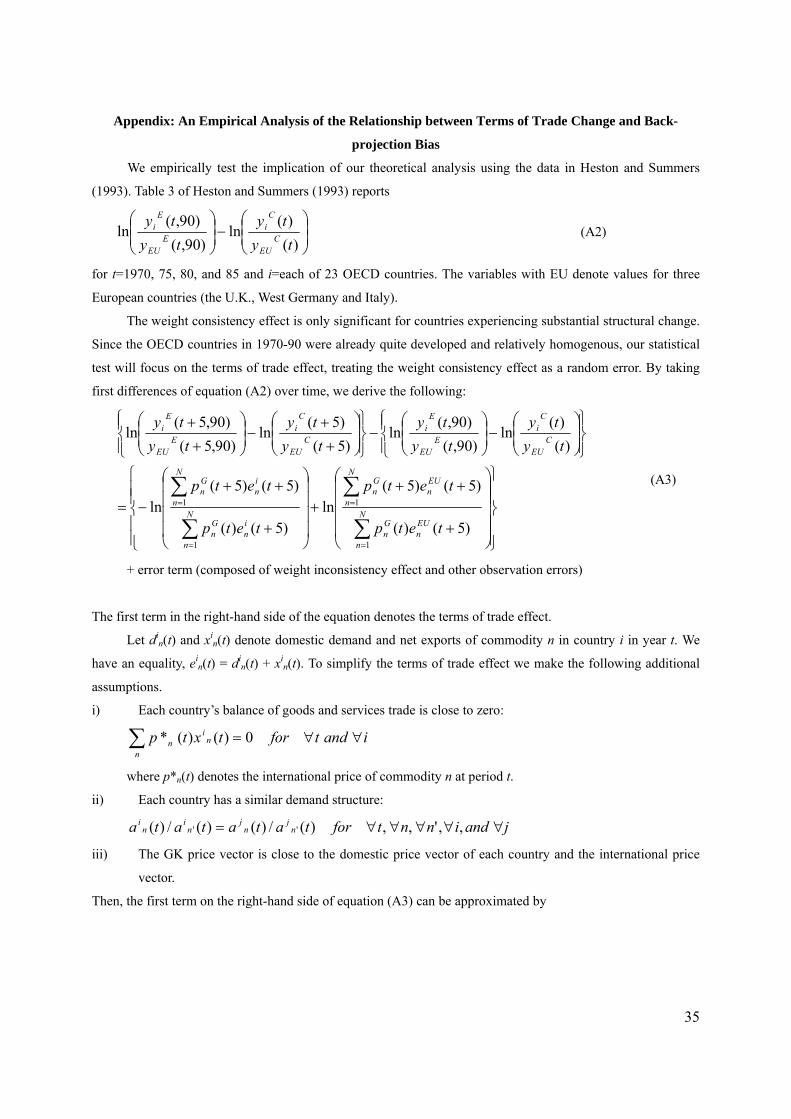
35

Appendix: An Empirical Analysis of the Relationship between Terms of Trade Change and Back-

projection Bias

We empirically test the implication of our theoretical analysis using the data in Heston and Summers

(1993). Table 3 of Heston and Summers (1993) reports

⎟⎟⎠

⎞⎜⎜⎝

⎛−⎟

⎟⎠

⎞⎜⎜⎝

⎛

)()(

ln)90,(

)90,(ln

tyty

tyty

CEU

Ci

EEU

Ei (A2)

for t=1970, 75, 80, and 85 and i=each of 23 OECD countries. The variables with EU denote values for three

European countries (the U.K., West Germany and Italy).

The weight consistency effect is only significant for countries experiencing substantial structural change.

Since the OECD countries in 1970-90 were already quite developed and relatively homogenous, our statistical

test will focus on the terms of trade effect, treating the weight consistency effect as a random error. By taking

first differences of equation (A2) over time, we derive the following:

⎪⎪⎭

⎪⎪⎬

⎫

⎪⎪⎩

⎪⎪⎨

⎧

⎟⎟⎟⎟

⎠

⎞

⎜⎜⎜⎜

⎝

⎛

+

+++

⎟⎟⎟⎟

⎠

⎞

⎜⎜⎜⎜

⎝

⎛

+

++−=

⎪⎭

⎪⎬⎫

⎪⎩

⎪⎨⎧

⎟⎟⎠

⎞⎜⎜⎝

⎛−⎟

⎟⎠

⎞⎜⎜⎝

⎛−

⎪⎭

⎪⎬⎫

⎪⎩

⎪⎨⎧

⎟⎟⎠

⎞⎜⎜⎝

⎛

+

+−⎟

⎟⎠

⎞⎜⎜⎝

⎛

+

+

∑

∑

∑

∑

=

=

=

=N

n

EUn

Gn

N

n

EUn

Gn

N

n

in

Gn

N

n

in

Gn

CEU

Ci

EEU

Ei

CEU

Ci

EEU

Ei

tetp

tetp

tetp

tetp

tyty

tyty

tyty

tyty

1

1

1

1

)5()(

)5()5(ln

)5()(

)5()5(ln

)()(

ln)90,(

)90,(ln

)5()5(

ln)90,5(

)90,5(ln

(A3)

+ error term (composed of weight inconsistency effect and other observation errors)

The first term in the right-hand side of the equation denotes the terms of trade effect.

Let din(t) and xi

n(t) denote domestic demand and net exports of commodity n in country i in year t. We

have an equality, ein(t) = di

n(t) + xin(t). To simplify the terms of trade effect we make the following additional

assumptions.

i) Each country’s balance of goods and services trade is close to zero:

iandtfortxtpn

ni

n ∀∀=∑ 0)()(*

where p*n(t) denotes the international price of commodity n at period t.

ii) Each country has a similar demand structure:

jandinntfortatatata nj

nj

ni

ni ∀∀∀∀∀= ,,',,)(/)()(/)( ''

iii) The GK price vector is close to the domestic price vector of each country and the international price

vector.

Then, the first term on the right-hand side of equation (A3) can be approximated by

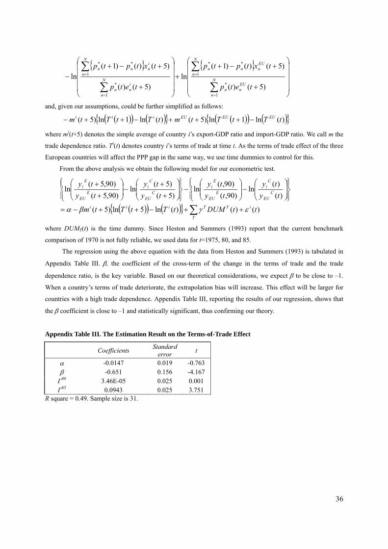
36

{ } { }

⎟⎟⎟⎟

⎠

⎞

⎜⎜⎜⎜

⎝

⎛

+

+−++

⎟⎟⎟⎟

⎠

⎞

⎜⎜⎜⎜

⎝

⎛

+

+−+−

∑

∑

∑

∑

=

=

=

=N

n

EUnn

N

n

EUnnn

N

n

inn

N

n

innn

tetp

txtptp

tetp

txtptp

1

*

1

**

1

*

1

**

)5()(

)5()()1(ln

)5()(

)5()()1(ln

and, given our assumptions, could be further simplified as follows:

( )( ) ( ){ } ( )( ) ( ){ })(ln1ln)5()(ln1ln)5( tTtTtmtTtTtm EUEUEUiii −+++−++−

where mi(t+5) denotes the simple average of country i’s export-GDP ratio and import-GDP ratio. We call m the

trade dependence ratio. Ti(t) denotes country i’s terms of trade at time t. As the terms of trade effect of the three

European countries will affect the PPP gap in the same way, we use time dummies to control for this.

From the above analysis we obtain the following model for our econometric test.

( )( ) ( ){ } )()()(ln5ln)5(

)()(

ln)90,(

)90,(ln

)5()5(

ln)90,5(

)90,5(ln

ttDUMtTtTtm

tyty

tyty

tyty

tyty

iT

T

Tiii

CEU

Ci

EEU

Ei

CEU

Ci

EEU

Ei

εγβα ++−++−=

⎪⎭

⎪⎬⎫

⎪⎩

⎪⎨⎧

⎟⎟⎠

⎞⎜⎜⎝

⎛−⎟

⎟⎠

⎞⎜⎜⎝

⎛−

⎪⎭

⎪⎬⎫

⎪⎩

⎪⎨⎧

⎟⎟⎠

⎞⎜⎜⎝

⎛

+

+−⎟

⎟⎠

⎞⎜⎜⎝

⎛

+

+

∑

where DUMT(t) is the time dummy. Since Heston and Summers (1993) report that the current benchmark

comparison of 1970 is not fully reliable, we used data for t=1975, 80, and 85.

The regression using the above equation with the data from Heston and Summers (1993) is tabulated in

Appendix Table III. β, the coefficient of the cross-term of the change in the terms of trade and the trade

dependence ratio, is the key variable. Based on our theoretical considerations, we expect β to be close to –1.

When a country’s terms of trade deteriorate, the extrapolation bias will increase. This effect will be larger for

countries with a high trade dependence. Appendix Table III, reporting the results of our regression, shows that

the β coefficient is close to –1 and statistically significant, thus confirming our theory.

Appendix Table III. The Estimation Result on the Terms-of-Trade Effect

Coefficients Standard error t

α -0.0147 0.019 -0.763β -0.651 0.156 -4.167Γ80 3.46E-05 0.025 0.001 Γ85 0.0943 0.025 3.751

R square = 0.49. Sample size is 31.