Hidden Markov models

Stat 518

Sp08

A Markov chain model

January data from Snoqualmie Falls, Washington, 1948-1983

325 dry and 791 wet days

Today wet Today dry

Yesterday wet 643 (543) 128 (223) 771

Yesterday dry 123 (223) 186 (91) 309

766 314 1080

€

(Rt | Rt −1,...,R1) ~ pRt −1,Rt

0 5 10 15

Dry period length (days)

1.00

0.10

0.01

Survival function

S(t) = 1 – Pr(Dry period ≤ t)

Dry period ~ Geom(1/(1-p00))

A spatial Markov model

Three sites, A, B and C, each observing 0 or 1. Notation: AB = (A=1,B=1,C=0)

Markov model:

Great Plains data1949-1984 (Jan-Feb)

€

P(Xt ≡ (XA,t ,XB,t ,XC,t ) = (i, j,k) | Xt −1 = (l,m,n),...,X1)

= plmn,ijk

Dry A B C AB AC BC ABC

Obs 718 1020 1154 957 866 752 728 657

MC 722 942 1076 1031 789 750 727 655

A hidden weather state

Two-stage model

Ct Markov chain, c states

(Rt|Ct,Rt-1,Ct-1,...,C1,R1) = (Rt|Ct)=t(Ct)

We observe only R1,...,RT.

C clusters similar rainfall patterns. In atmospheric science called a weather state

Likelihood

|C|=3, T=100, |CT| = 5.2 x 1047

Forward algorithm: unravel sum recursively

€

L(θ) = Lc∈CT

∑ p(ri | ci;θ)p(ci;θ)i=1

T∏∑

€

α t (j) = Pr(R1,...,Rt ,Ct = j)

= α t −1(i)i=1

|C|∑ πt (j)pi,j

€

L(θ) = αTj=1

|C|∑ (j)

Computational algorithm

Lystig (2001): Write

€

L(θ) = Pr(R1,...,RT;θ) = Pr(Rt | Rt −1t =1

T∏ ,...,R1;θ)

€

λ t (j) = Pr(Rt ,Ct = j | Rt −1,...,R1)

=λt −1(i)πt (j)pi,j

Λ t −1i=1

|C|

∑

€

Λt = λt (j)j=1

|C|∑ = Pr(Rt | Rt −1,...,R1)

€

l (θ) = logL(θ) = log Λ tt =1

T∑

Estimating standard errors

The Lystig recursions enable easy calculation of first and second derivatives of the log likelihood, which can be used to estimate standard errors of maximum likelihood estimates of .

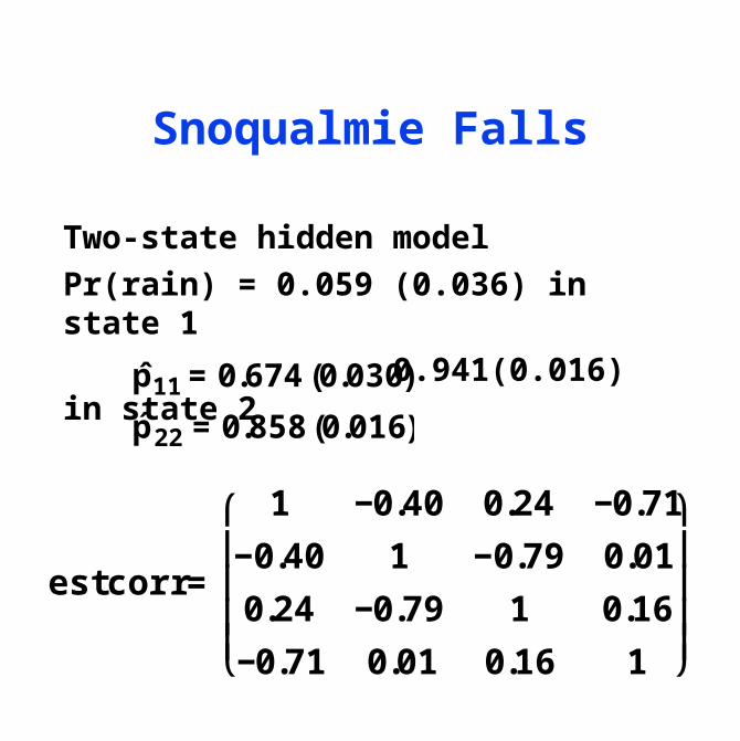
Snoqualmie Falls

Two-state hidden model

Pr(rain) = 0.059 (0.036) in state 1

0.941(0.016) in state 2

€

ˆ p 11 = 0.674 (0.030)

ˆ p 22 = 0.858 (0.016)

€

est corr =

1 −0.40 0.24 −0.71

−0.40 1 −0.79 0.01

0.24 −0.79 1 0.16

−0.71 0.01 0.16 1

⎛

⎝

⎜ ⎜ ⎜ ⎜

⎞

⎠

⎟ ⎟ ⎟ ⎟

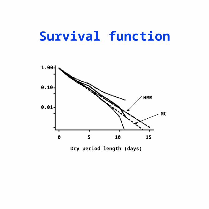
Survival function

0 5 10 15

Dry period length (days)

1.00

0.10

0.01MC

HMM

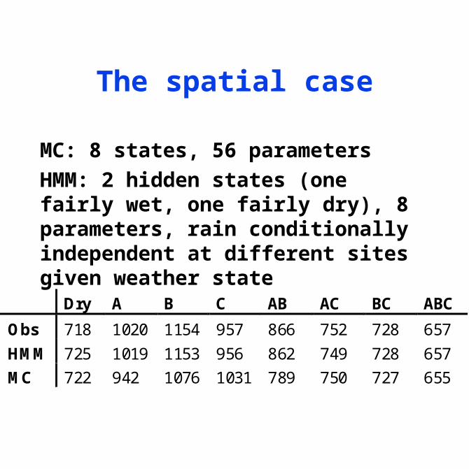
The spatial case

MC: 8 states, 56 parameters

HMM: 2 hidden states (one fairly wet, one fairly dry), 8 parameters, rain conditionally independent at different sites given weather state

Dry A B C AB AC BC ABC

Obs 718 1020 1154 957 866 752 728 657

HMM 725 1019 1153 956 862 749 728 657

MC 722 942 1076 1031 789 750 727 655

Nonstationary transition probabilities

Meteorological conditions may affect transition probabilities

At-1 At

Ct-2 Ct-1 Ct

Rt-2 Rt-1 Rt

€

logpij (t)

1− pij (t)

⎛

⎝ ⎜

⎞

⎠ ⎟ = α ij + βj

TAt

A model for Western Australia rainfall

1978–1987 (1992) winter (May– Oct) daily rainfall at 30 stations

Atmospheric variables in model: E-W gradient in 850 hPa geopotential height, mean sea level pressure, N-S gradient in sea-level pressure

Final model has six weather states (BIC and other diagnostics)

Rain probabilities

Spatial dependence