high-dimensional brain: a tool for encoding and rapid
TRANSCRIPT

Bull Math Biolhttps://doi.org/10.1007/s11538-018-0415-5
SPECIAL ISSUE: MODELLING BIOLOGICAL EVOLUTION: DEVELOPING NOVEL APPROACHES
High-Dimensional Brain: A Tool for Encoding andRapid Learning of Memories by Single Neurons
Ivan Tyukin1,2 · Alexander N. Gorban1 · Carlos Calvo3 ·Julia Makarova4,5 · Valeri A. Makarov3,5
Received: 16 October 2017 / Accepted: 4 March 2018© The Author(s) 2018
Abstract Codifying memories is one of the fundamental problems of modern Neuro-science. The functionalmechanismsbehind this phenomenon remain largely unknown.Experimental evidence suggests that some of the memory functions are performed bystratified brain structures such as the hippocampus. In this particular case, single neu-rons in the CA1 region receive a highly multidimensional input from the CA3 area,which is a hub for information processing. We thus assess the implication of the abun-dance of neuronal signalling routes converging onto single cells on the informationprocessing. We show that single neurons can selectively detect and learn arbitraryinformation items, given that they operate in high dimensions. The argument is basedon stochastic separation theorems and the concentration of measure phenomena. Wedemonstrate that a simple enough functional neuronal model is capable of explaining:(i) the extreme selectivity of single neurons to the information content, (ii) simultane-ous separation of several uncorrelated stimuli or informational items from a large set,and (iii) dynamic learning of new items by associating them with already “known”ones. These results constitute a basis for organization of complex memories in ensem-bles of single neurons. Moreover, they show that no a priori assumptions on the
B Ivan [email protected]
1 Department of Mathematics, University of Leicester, University Road, Leicester LE1 7RH, UK
2 Saint-Petersburg State Electrotechnical University, Prof. Popova Str. 5, Saint Petersburg, Russia
3 Instituto de Matemática Interdisciplinar, Faculty of Mathematics, Universidad Complutense deMadrid, Avda Complutense s/n, 28040 Madrid, Spain
4 Department of Translational Neuroscience, Cajal Institute, CSIC, Madrid, Spain
5 Lobachevsky State University of Nizhny Novgorod, Gagarin Ave. 23, Nizhny Novgorod,Russia 603950
123

I. Tyukin et al.
structural organization of neuronal ensembles are necessary for explaining basic con-cepts of static and dynamic memories.
Keywords Neural memories · Single-neuron learning · Perceptron · Stochasticseparation theorems
1 Introduction
The human brain is arguably among the most sophisticated and enigmatic naturecreations. Over millions of years it has evolved to amass billions of neurons, featuringon average 86×109 cells (Herculano-Houzel 2012). This remarkable figure is severalorders of magnitude higher than that of the most mammals and several times largerthan in primates (Herculano-Houzel 2011). While measuring roughly 2% of the bodymass, the human brain consumes about 20% of the total energy (Clark and Sokoloff1999).
The significant metabolic cost associated with a larger brain in humans, as opposedto mere body size—a path that great apes might have evolved (Herculano-Houzel2011), must be justified by evolutionary advantages. Some of the benefits may berelated to the development of a remarkably important social life in humans. This, inparticular, requires extensive abilities in the formationof complexmemories. Indirectlythis hypothesis is supported by the significant difference among species in the numberof neurons in the cortex (Herculano-Houzel 2009) and the hippocampus (Andersenet al. 2007). For example, in the CA1 area of the hippocampus there are 0.39 × 10⁶
pyramidal neurons in rats, 1.3 × 10⁶ in monkeys, and 14 × 106 in humans.Evolutionary implications in relation to cognitive functions have been widely dis-
cussed in the literature (see, e.g., Platek et al. 2007; Sherwood et al. 2012; Sousa et al.2017). Recently, it has been shown that in humans new memories can be learnt veryrapidly by supposedly individual neurons from a limited number of experiences (Isonet al. 2015). Moreover, some neurons can exhibit remarkable selectivity to complexstimuli, the evidence that has led to debates around the existence of the so-called “grandmother” and “concept” cells (Quiroga et al. 2005;Viskontas et al. 2009;Quiroga 2012),and their role as elements of a declarative memory. These findings suggest that notonly the brain can learn rapidly but also it can respond selectively to “rare” individualstimuli. Moreover, experimental evidence indicates that such a cognitive functionalitycan be delivered by single neurons (Ison et al. 2015; Quiroga et al. 2005; Viskontaset al. 2009). The fundamental questions, hence, are: How is this possible? and Whatcould be the underlying functional mechanisms?
Recent theoretical advances achieved within the Blue Brain Project show that thebrain can operate in many dimensions (Reimann et al. 2017). It is claimed that thebrain has structures operating in up to eleven dimensions. Groups of neurons canform the so-called cliques, i.e., networks of specially interconnected neurons thatgenerate precise representations of geometric objects. Then the dimension growswith the number of neurons in the clique. Multidimensional representation of spa-tiotemporal information in the brain is also implied in the concept of generalizedcognitive maps (see, e.g., Villacorta-Atienza et al. 2015; Calvo et al. 2016; Villacorta-
123

High-Dimensional Brain: A Tool for. . .
Atienza et al. 2017). Within this theory, spatiotemporal relations between objects inthe environment are encoded as static (cognitive) maps and represented as elementsof an n-dimensional space (n � 1). The cognitive maps as information items can belearnt, classified, and retrieved on demand (Villacorta-Atienza and Makarov 2013).However, the questions concerning how the brain or individual neurons can distin-guish among a huge number of different maps and select an appropriate one remainunknown.
In this work we propose that brain areas with a predominant laminar topologyand abundant signalling routes simultaneously converging on individual cells (e.g.,the hippocampus) are propitious for a high-dimensional processing and learning ofcomplex information items. We show that a canonical neuronal model, the percep-tron Rosenblatt (1962), in combination with a Hebbian-type of learning may provideanswers to the above-mentioned fundamental questions. In particular, starting fromstochastic separation theorems (Gorban and Tyukin 2017, 2018) we demonstrate thatindividual neurons gathering multidimensional stimuli through a sufficiently largenumber of synaptic inputs can exhibit extreme selectivity either to individual infor-mation items or to groups of items. Moreover, neurons are capable of associating andlearning uncorrelated information items. Thus, a large number of signalling routessimultaneously converging on a large number of single cells, as it is widely observedin laminar brain structures, translates into a natural environment for rapid formationand maintenance of extensive memories. This is vital for social life and hence mayconstitute a significant evolutionary advantage, albeit, at the cost of high metabolicexpenditure.
2 Fundamental Problems of Encoding Memories
Different brain structures, such as the hippocampus, have a pronounced laminar orga-nization. For example, the CA1 region of the hippocampus is constituted by a palisadeof morphologically similar pyramidal cells oriented with their main axis in paralleland forming a monolayer (Fig. 1a). The major excitatory input to these neurons comesthrough Schaffer collaterals from the CA3 region (Amaral and Witter 1989; Ishizukaet al. 1990; Wittner et al. 2007), which is a hub routing information among manybrain structures. Each CA3 pyramidal neuron sends an axon that bifurcates and leavesmultiple collaterals in theCA1with dominant parallel orientation (Fig. 1b). This topol-ogy allows multiple parallel axons conveying multidimensional “spatial” informationfrom one area (CA3) simultaneously leave synaptic contacts on multiple neurons inanother area (CA1). Thus, we have simultaneous convergence and divergence of theinformation content (Fig. 1b, right).
Experimental findings show that multiple CA1 pyramidal cells distributed in therostro-caudal direction are activated near-synchronously by assemblies of simultane-ously firing CA3 pyramidal cells (Ishizuka et al. 1990; Li et al. 1994; Benito et al.2014). Thus, an ensemble of single neurons in the CA1 can receive simultaneously thesame synaptic input (Fig. 1b, left). Since these neurons have different topology andfunctional connectivity (Finnerty and Jefferys 1993), their response to the same inputcan be different. Moreover, experimental in vivo results show that long-term poten-
123

I. Tyukin et al.
C
A B
1 2 3
stim
ulus
response
CA3
CA1
output
Sch. input
CA3Schaffer collaterals
one item learning retrieval
Fig. 1 General principles of encodingmemories by single neurons in laminar structures. a Laminar organi-zation of the CA3 and CA1 areas in the hippocampus facilitates multiple parallel synaptic contacts betweenneurons in these areas bymeans of Schaffer collaterals. bAxons fromCA3 pyramidal neurons bifurcate andpass through the CA1 area in parallel (left panel) giving rise to the convergence–divergence of the informa-tion content (right panel). Multiple CA1 neurons receive multiple synaptic contacts from CA3 neurons. cSchematic representation of three memory encoding schemes. (1) Selectivity. A neuron (shown in yellow)receives inputs frommultiple presynaptic cells that code different information items. It detects (responds to)only one stimulus (purple trace), whereas rejecting the others. (2) Clustering. Similar to 1, but now a neuron(shown in pink) detects a group of stimuli (purple and blue traces) and ignores the others. (3) Acquiringmemories. A neuron (shown in green) learns dynamically a new memory item (blue trace) by associatingit with a know one (purple trace) (Color figure online)
tiation can significantly increase the spike transfer rate in the CA3–CA1 pathway(Fernandez-Ruiz et al. 2012). This suggests that the efficiency of individual synapticcontacts can be increased selectively.
In this work we will follow conventional and rather general functional representa-tion of signalling in the neuronal pathways. We assume that upon receiving an input, aneuron can either generate a response or remain silent. Forms of the neuronal responsesas well as the definitions of synaptic inputs vary from onemodel to another. Therefore,here we adopt a rather general functional approach. Under a stimulus we understand
123

High-Dimensional Brain: A Tool for. . .
a number of excitations simultaneously (or within a short time window) arriving to aneuron through several axones and thus transmitting some “spatially coded” informa-tion items (Benito et al. 2016). If a neuron responds to a stimulus (e.g., generates outputspikes or increases its firing rate), we then say that the neuron detects the informationalcontent of the given stimulus.
We follow the standard machine learning assumptions (Vapnik and Chapelle 2000;Cucker and Smale 2002). The stimuli are generated in accordance with some dis-tribution or a set of distributions (“Outer World Models”). All stimuli that a neuronmay receive are samples from this distribution. The sampling itself may be a com-plicated process, and for simplicity we assume that all samples are identically andindependently distributed (i.i.d.). Once a sample is generated, a stimuli sub-sample isindependently selected for testing purposes. If more than one neuron is considered,we will assume that a rule (or a set of rules) is in place that determines how a neuronis selected from the set. The rules can be both deterministic and randomized. In thelatter case we will specify this process.
Let us now pose the following fundamental questions related to the informationencoding and formation of memories by single neurons and their ensembles in lami-nated brain structures:
1. Selectivity: detection of one stimulus from a set (Fig. 1C.1) Pick an arbitrarystimulus from a reasonably large set such that a single neuron from a neuronalensemble detects this stimulus. Then what is the probability that this neuron isstimulus-specific, i.e., it rejects all the other stimuli from the set?
2. Clustering: detection of a group of stimuli from a set (Fig. 1C.2) Within a setof stimuli we select a smaller subset, i.e., a group of stimuli. Then what is theprobability that a neuron detecting all stimuli from this subset stays silent for allremaining stimuli in the set?
3. Acquiring memories: learning new stimulus by associating it with one alreadyknown (Fig. 1C.3) Let us consider two different stimuli s1 and s2 such that fort ≤ t0 they do not overlap in time and a neuron detects s1, but not s2. In the nextinterval (t0, t1], t1 > t0 the stimuli start to overlap in time (i.e., they stimulate theneuron together). For t > t1 the neuron receives only stimulus s2. Then what isthe probability that for some t2 ≥ t1 the neuron detects s2?
These questions are in the core of a broad range of puzzling phenomena reported inIson et al. (2015), Quiroga et al. (2005), Viskontas et al. (2009). Inwhat followswewillshow that, remarkably, these three non-trivial fundamental questions can be answeredwithin a simple classical modeling framework, whereby a neuron is represented by amere perceptron equipped with a Hebbian-type of learning.
3 Formal Statement of the Problem
In this sectionwe specify the information content to be processed by neurons and definea mathematical model of a generic neuron equipped with synaptic plasticity. Beforegoing any further, let us first introduce notational agreements used throughout the text.Given two vectors x, y ∈ R
n , their inner product 〈x, y〉 is: 〈x, y〉 = ∑ni=1 xi yi . If
x ∈ Rn then ‖x‖ stands for the usual Euclidean norm of x: ‖x‖ = 〈x, x〉1/2. By
123

I. Tyukin et al.
time
s1 s2 sMx1 =
x2 =..
.
xM =
S(t) =M
i=1
si(t, xi)
. . .
ΔT
τij + ΔTτij
f
Fig. 2 Codification of high-dimensional information by a neuron. Each of M stimuli comprises of the“spatial” information, xi ∈ R
n , (e.g., M images) conducted through n axons (in yellow) and the temporalpart, c(t − τi, j ), reflecting the times of stimuli presentation. A neuron (in blue) receives the stimuli andgenerates responses determined by some transfer function f (Color figure online)
Bn(1) = {x ∈ Rn| ‖x‖ ≤ 1} we denote a unit n-ball centered at the origin; V(�) is
the Lebesgue volume of� ⊂ Rn , and |M| is the cardinality of a finite setM. Symbol
C(D), D ⊆ Rm stands for the space of continuous real-valued functions on D.
3.1 Information Content and Classes of Stimuli
Weassume that a neuron receives and processes a large but finite set of different stimulicodifying different information items:
S = {si }. (1)
Figure 2 illustrates schematically the information flow. Each individual stimulus iis modeled by a function s : R × R
n → Rn :
s(t, xi ) = xi∑
j
c(t − τi, j ), (2)
where xi ∈ Rn \{0} is the stimulus content codifying the information to be transmitted
over n individual “axons”. An example of an information item could be an l×k image(see Fig. 2). In this case the dimension of each information item is n = l × k.
123

High-Dimensional Brain: A Tool for. . .
In Eq. (2) the function c(·) defines the stimulus context, i.e., the time window whenthe stimulus arrives to the neuron. For the sake of simplicity we use a rectangularwindow:
c(t) ={1, if t ∈ [0,ΔT ]0, otherwise,
(3)
where ΔT > 0 is the window length. The time instants of the stimulus presentations,τi, j , are ordered and satisfy:
τi, j+1 > τi, j + ΔT, ∀ j. (4)
Different stimuli arriving to the neuron are added linearly on the neuronal mem-brane. Thus, the overall neuronal input S can be written as:
S(t) =∑
i, j
xi c(t − τi, j ). (5)
We assume that the information content of stimuli (5) and (2), i.e., vectors xi aredrawn i.i.d. from some distribution. For convenience, we partition all informationitems into two sets:
M = {x1, . . . , xM }, Y = {xM+1, . . . , xM+m}, (6)
whereM is large but finite andm ≥ 1 is in general smaller thanM . The setM containsa background content for a given neuron, whereas the set Y models the informationalcontent relevant to the task at hand. In other words, to accomplish a static memorytask the neuron should be able to detect all elements from Y and to reject all elementsfromM.
The setsM and Y give rise to the corresponding subsets of stimuli:
S(M) = {si ∈ S | si (·) = s(·, xi ), xi ∈ M},S(Y) = {si ∈ S | si (·) = s(·, xi ), xi ∈ Y}. (7)
3.2 Neuronal Model
To stay within functional description of the information processing let us considerthe most basic class of model neurons, a perceptron (Rosenblatt 1962). A singleneuron receives a stimulus s(t, x) through n synaptic inputs (Fig. 2) and its membranepotential, y ∈ R, is given by
y(s,w) = 〈w, s〉, (8)
where w ∈ Rn is a vector of the synaptic weights. The neuron generates a response,
v ∈ R, according to:v(s,w, θ) = f (y(s,w) − θ), (9)
123

I. Tyukin et al.
where θ ∈ R is the “firing” threshold and f : R → R is the transfer function (Fig. 2):f ∈ C(R), f is locally Lipschitz, f (u) = 0 for u ∈ (−∞, 0], and f (u) > 0 foru ∈ (0,∞).
Model (8), (9) captures the summation of postsynaptic potentials and the thresholdnature of the neuronal activation but disregards the specific dynamics accounted forin other more advanced models. Nevertheless, as we will show in Sect. 4, this phe-nomenological model is already sufficient to explain the fundamental properties ofinformation processing discussed in Sect. 2.
3.3 Synaptic Plasticity
In addition to the basic neuronal response mechanism (Sect. 3.2), we also model thesynaptic plasticity. The description adopted here relies on the neuronal firing rate andHebbian learning. Such a learning rule implies that the dynamics of w should dependon the product of the input signal, s, and the neuronal output, v. We thus arrive to amodified classical Oja rule (Oja 1982):
w = αv(s,w, θ)y(s,w) (s − wy(s,w)) ,
w(t0) =w0 ∈ Rn, w0 �= 0,
(10)
where α > 0 defines the relaxation time. The multiplicative term v in (10) ensures thatplastic changes of w occur only when an input stimulus evokes a nonzero neuronalresponse. The fact thatw0 �= 0 reflects the assumption that synaptic connections havealready been established, albeit their efficacy could be subjected to plastic changes.In addition to capturing general principle of the classical Hebbian rule, model (10)guarantees that synaptic weights w are bounded in forward time (see “Appendix A”)and hence conforms with physiological plausibility.
4 Formation of Memories in High Dimensions
In Sect. 2 we formulated three fundamental problems of organization of memories inlaminar brain structures. Let us now show how they can be treated given that pyramidalneurons operate in high dimensions.
To formalize the analysis let U be a subset of the stimulus set S. A neuron (8), (9)parameterized by (w, θ) partitions the set U into the following subsets:
Activated(U , (w, θ)) ={si ∈ U | ∃ t≥t0 : v(si (t),w, θ) > 0},Silent(U , (w, θ)) ={si ∈ U | v(si (t),w, θ) = 0 ∀ t ≥ t0}. (11)
The first set corresponds to the stimuli detected by the neuron, while the second onecollects background stimuli.
123
High-Dimensional Brain: A Tool for. . .
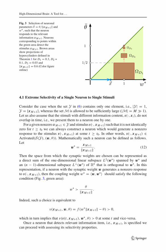
Fig. 3 Selection of neuronalparameters θ = θ/‖xM+1‖ andw∗, such that the neuronresponds to the relevantinformation xM+1. Neuronscorresponding to points withinthe green area detect thestimulus xM+1. Brown areasshow projections ofhypercylinders defined inTheorem 1 for D1 = 0.3, D2 =0.1, D3 = 0.03 and‖xM+1‖ = 0.6 (Color figureonline)
ΩD2
ΩD1
1/2
1
1
ΩD3
θ
x w∗
4.1 Extreme Selectivity of a Single Neuron to Single Stimuli
Consider the case when the set Y in (6) contains only one element, i.e., |Y| = 1,Y = {xM+1}, whereas the setM is allowed to be sufficiently large (|M| = M � 1).Let us also assume that the stimuli with different information content, s(·, xi ), do notoverlap in time, i.e., we present them to a neuron one by one.
For a given nonzero xM+1 ∈ Y and stimulus s(·, xM+1) such that it is not identicallyzero for t ≥ t0 we can always construct a neuron which would generate a nonzeroresponse to the stimulus s(·, xM+1) at some t ≥ t0. In other words, s(·, xM+1) ∈Activated(S(Y), (w, θ)). Mathematically such a neuron can be defined as follows.Let
w∗ = xM+1
‖xM+1‖ . (12)
Then the space from which the synaptic weights are chosen can be represented asa direct sum of the one-dimensional linear subspace L‖(w∗) spanned by w∗ andan (n − 1)-dimensional subspace L⊥(w∗) of R
n that is orthogonal to w∗. In thisrepresentation, if a neuron with the synaptic weight w generates a nonzero responseto s(·, xM+1), then the coupling weight w∗ = 〈w,w∗〉 should satisfy the followingcondition (Fig. 3, green area):
w∗ >θ
‖xM+1‖ .
Indeed, such a choice is equivalent to
v(xM+1,w, θ) = f (w∗‖xM+1‖ − θ) > 0,
which in turn implies that v(s(t, xM+1),w∗, θ) > 0 at some t and vice-versa.
Once a neuron that detects relevant information item, i.e., xM+1, is specified wecan proceed with assessing its selectivity properties.
123

I. Tyukin et al.
t
y3(t)
y2(t)
y1(t)θ1
θ3
θ2
S(t)
t
t
t
Fig. 4 Example of selective neuronal responses to stimulation with different (30×38)-pixels images (onlyfirst few stimulus are shown in the time line). Each neuron responds to its own (relevant) stimulus only andrejects the other (background) stimuli
Definition 1 (Neuronal Selectivity)We say that a neuron is selective to the informationcontent Y iff it detects the relevant stimuli from the set S(Y) and ignores all the othersfrom the set S(M).
The notion of selectivity, as stated in Definition 1, could be relaxed to account forpartial detection and rejection of information content fromY andM, respectively. Thisnaturally gives rise to various levels of neuronal selectivity determined, for instance, bythe proportion of elements fromM that correspond to stimuli that have been rejected.As we will see below, different admissible pairs (w, θ) (Fig. 3) produce differentselectivity levels. The closer to the bisector, the higher the selectivity. One can pickan arbitrary firing threshold θ ≥ 0 and select the synaptic efficiency at t = t0 as:
w(t0) = θ + ε
‖xM+1‖w∗ + w⊥, ε > 0, w⊥ ∈ L⊥. (13)
It can be shown (see “Appendix A”) that if the stimulus s(·, xM+1) is persistent overtime and w(t0) satisfies (13) then synaptic efficiency w(t,w0) converges asymptoti-cally (as t → ∞) to:
w∞ ={w∗, if θ < ‖xM+1‖
θ‖xM+1‖w∗ + w⊥∞, if θ ≥ ‖xM+1‖, (14)
where w⊥∞ is an element of L⊥.Figure 4 shows typical responses of neurons parameterized by different pairs (w, θ)
and subjected to stimulation by different information items xi . Here xi correspond to(30×38)-pixels color images (i.e., xi ∈ R
3420). Firing thresholds θ have been chosenat random, and weights w have been set in accordance with (13) with the first three
123

High-Dimensional Brain: A Tool for. . .
images serving as the relevant information items for the three corresponding neurons.No plastic changes inw were allowed. The neurons detect their own (relevant) stimuli,as expected. Moreover, they do not respond to the stimulation by other backgroundinformation items (4 out of 103 images are shown in Fig. 4). Thus, the neurons indeedexhibit high stimulus selectivity.
The following theorem provides theoretical justification for these observations.
Theorem 1 Let elements of the sets M and Y be i.i.d. random vectors drawn fromthe equidistribution in Bn(1). Consider the sets of stimuli S(M) and S(Y) specifiedby (7). Let (w, θ) be the neuron parameters such that
sM+1 ∈ Activated(S(Y), (w, θ)) and 0 < θ < ‖w‖.
Then:
1. The probability that the neuron is silent for all background stimuli si ∈ S(M) isbounded from below by:
P(si ∈ Silent(S(M), (w, θ)) ∀si ∈ S(M)∣∣ w, θ) ≥
≥[
1 − 1
2
(
1 − θ2
‖w‖2) n
2]M
.(15)
2. There is a family of sets parametrized by D (0 < D < min{ 12 , ‖xM+1‖}):
ΩD ={(w, θ)
∣∣ ‖w − w∗‖ < D, D ≤ ‖xM+1‖ − θ ≤ 2D
}, (16)
where w∗ = xM+1/‖xM+1‖, such that sM+1 ∈ Activated(S(Y), (w, θ)), for(w, θ) ∈ ΩD and
P(si ∈ Silent(S(M), (w, θ)) ∀si ∈ S(M)
∣∣ ∀(w, θ) ∈ ΩD
) ≥
≥ maxε∈(0,1−2D)
(1 − (1 − ε)n)
[
1 − 1
2ρ(ε, D)
n2
]M (17)
where
ρ(ε, D) = 1 −(1 − ε − 2D
1 + D
)2
.
The proof is provided in “Appendix B”.
Remark 1 For an admissible fixed D > 0, the volume V(ΩD) > 0. Therefore, theestimate provided by Theorem 1 is robust to small perturbations of (w, θ), and slightfluctuations of neuronal characteristics are not expected to affect neuronal functional-ity.
123

I. Tyukin et al.
A Bse
lect
ivity
(%)
neuron dimension, n neuron dimension, n
mem
ory
capa
city
101
102
103
104
105
4 8 12 16 2010 20 300
20
40
60
80
100hypercubeunit ball
100.33n
100.14n
hypercube
theoreticalunit ball
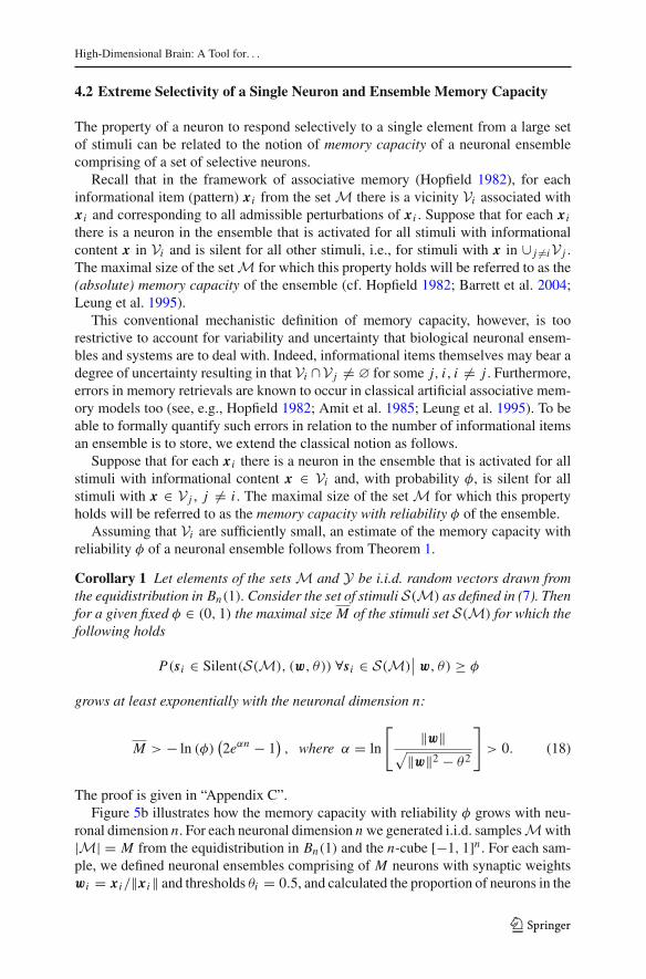
Fig. 5 Extreme selectivity to stimuli and memory capacity of single neurons. a Stimulus selectivity vsthe neuron dimension. The selectivity index steeply increases for n ∈ [10, 20]. For n > 20 practicallyall neurons become selective to a set of 103 random stimuli. b Memory capacity with reliability 0.95 ofa neuronal ensemble versus the neuron dimension. For both types of stimuli the memory capacity growsexponentially (straight lines show regressions)
Remark 2 Theorem 1 (part 2) specifies a non-iterative procedure for constructing setsof selective neurons. Such neurons detect given stimuli and reject the others, withhigh probability. Figure 3 (in brown) shows examples of three projections of thehypercylinders (16) ensuring robust selective stimulus detection. The smaller is thecylinder, the higher is the selectivity.
To illustrateTheorem1numericallywefixed the neuronal dimensionality parametern and generated two random sets of information items comprising of 103 elementseach, i.e., {xi }103i=1. One set was sampled from the equidistribution in a unit ball Bn(1)centered at the origin (i.e., ‖xi‖2 ≤ 1), and the other from the equidistribution in thehypercube ‖xi‖∞ ≤ 1 (a product distribution). For each set of informational items, aneuronal ensemble of 103 single neurons parameterized by (wi , θi ) was created. Eachneuron was assigned fixed firing threshold θi = 0.5, i = 1, . . . , 103, whereas thesynaptic efficiencies were set as wi = (θi + ε)xi/‖xi‖, ε = 0.05. For these neuronalensembles and their corresponding stimuli sets we evaluated output of each neuronand assessed the neuronal selectivity (see Def. 1). The procedure was repeated 10times. This was followed by evaluation of the frequencies of selective neurons in thepool for each n.
Figure 5a shows frequencies of selective neurons in an ensemble, for 103 stimulitaken from: i) a unit ball (red), ii) a hypercube (blue), and iii) the estimate providedby Theorem 1 (dashed). For n small (n < 6) neurons exhibit no selectivity, i.e.,they confuse different stimuli and generate nonspecific responses. As expected, whenneuronal dimensionality, n, increases, the neuronal selectivity increases rapidly; andat around n = 20 it approaches 100%.
123
High-Dimensional Brain: A Tool for. . .
4.2 Extreme Selectivity of a Single Neuron and Ensemble Memory Capacity
The property of a neuron to respond selectively to a single element from a large setof stimuli can be related to the notion of memory capacity of a neuronal ensemblecomprising of a set of selective neurons.
Recall that in the framework of associative memory (Hopfield 1982), for eachinformational item (pattern) xi from the set M there is a vicinity Vi associated withxi and corresponding to all admissible perturbations of xi . Suppose that for each xithere is a neuron in the ensemble that is activated for all stimuli with informationalcontent x in Vi and is silent for all other stimuli, i.e., for stimuli with x in ∪ j �=iV j .The maximal size of the setM for which this property holds will be referred to as the(absolute) memory capacity of the ensemble (cf. Hopfield 1982; Barrett et al. 2004;Leung et al. 1995).
This conventional mechanistic definition of memory capacity, however, is toorestrictive to account for variability and uncertainty that biological neuronal ensem-bles and systems are to deal with. Indeed, informational items themselves may bear adegree of uncertainty resulting in that Vi ∩V j �= ∅ for some j, i , i �= j . Furthermore,errors in memory retrievals are known to occur in classical artificial associative mem-ory models too (see, e.g., Hopfield 1982; Amit et al. 1985; Leung et al. 1995). To beable to formally quantify such errors in relation to the number of informational itemsan ensemble is to store, we extend the classical notion as follows.
Suppose that for each xi there is a neuron in the ensemble that is activated for allstimuli with informational content x ∈ Vi and, with probability φ, is silent for allstimuli with x ∈ V j , j �= i . The maximal size of the set M for which this propertyholds will be referred to as the memory capacity with reliability φ of the ensemble.
Assuming that Vi are sufficiently small, an estimate of the memory capacity withreliability φ of a neuronal ensemble follows from Theorem 1.
Corollary 1 Let elements of the sets M and Y be i.i.d. random vectors drawn fromthe equidistribution in Bn(1). Consider the set of stimuli S(M) as defined in (7). Thenfor a given fixed φ ∈ (0, 1) the maximal size M of the stimuli set S(M) for which thefollowing holds
P(si ∈ Silent(S(M), (w, θ)) ∀si ∈ S(M)∣∣ w, θ) ≥ φ
grows at least exponentially with the neuronal dimension n:
M > − ln (φ)(2eαn − 1
), where α = ln
[‖w‖
√‖w‖2 − θ2
]
> 0. (18)
The proof is given in “Appendix C”.Figure 5b illustrates how the memory capacity with reliability φ grows with neu-
ronal dimension n. For each neuronal dimension n we generated i.i.d. samplesMwith|M| = M from the equidistribution in Bn(1) and the n-cube [−1, 1]n . For each sam-ple, we defined neuronal ensembles comprising of M neurons with synaptic weightswi = xi/‖xi‖ and thresholds θi = 0.5, and calculated the proportion of neurons in the
123

I. Tyukin et al.
ensemble that are activated by each stimulus. If the proportionwas smaller than 0.05 ofthe total number of neurons, we incremented the value of M , generated a new sampleM with increased cardinality M , and repeated the experiment. The values of M cor-responding to samples at which the process stopped have been recorded and retained.These constituted empirical estimates of the maximal number of stimuli for which theproportion of neurons responding to a single stimulus is at most 0.05 = 1−φ. Figure5b shows empirical means of such numbers for the unit ball and in the hypercube.As follows from these observations, memory capacity grows exponentially with theneuron dimension in both cases. Such a fast growth can easily cover quite exigentmemory necessities.
4.3 Selectivity of a Single Neuron to Multiple Stimuli
To organize memories, the ability to associate different information items is essential(Fig. 1C2). To determine if such associations are feasible at the level of single neuronswe assess neuronal selectivity to multiple stimuli. In particular, we consider the setY [Eq. (6)] containing m > 1 random vectors: Y = {xM+1, . . . , xM+m}. As in Sect.4.1, here we assume that all stimuli do not overlap in time and arrive to the neuronseparately. The question of interest is: Can we find a neuron [i.e., parameters (w, θ)],such that it would generate a nonzero response to all si ∈ S(Y) and, with high enoughprobability, would be silent to all si ∈ S(M)?
Below we will show that this is indeed possible, provided that the neuronal dimen-sionality, n, is large enough. Moreover, the separation can be achieved by a neuronwith the vector of synaptic weights, w = w∗, closely aligned with the mean vector ofthe stimulus set Y:
x = 1
m
m∑
i=1
xM+i , w∗ = x‖x‖ . (19)
This vector points to the center of the group to be separated from the set M. In lowdimensions, e.g., when n = 2, such functionality appears to be extremely unlikely.However, high-dimensional neurons can accomplish this task with probability closeto one. Formal statement of this property is provided in Theorem 2.
Theorem 2 Let elements of the sets M and Y be i.i.d. random vectors drawn fromthe equidistribution in Bn(1). Consider the sets of stimuli S(M) and S(Y) specifiedby (7) and let D, ε, δ ∈ (0, 1) be chosen such that
θ∗ = (1 − ε)3 − δ(m − 1)√m(1 − ε)[1 − ε + δ(m − 1)] ∈ (D, 1). (20)
Let w∗ = x/‖x‖ and consider the set:
ΩD ={(w, θ)
∣∣ ‖w − w∗‖ < D, θ ∈ (0, θ∗ − D]
}.
123
High-Dimensional Brain: A Tool for. . .
Then
P([si ∈ Activated(S(Y),w, θ) ∀ si ∈ S(Y)] &
[si ∈ Silent(S(M),w, θ) ∀ si ∈ S(M)]∣∣∣ (w, θ) ∈ ΩD
)≥ p(ε, δ, D,m),
(21)
where
p(ε, δ, D,m) =(1 − (1 − ε)n)mm−1∏
d=1
(
1 − d(1 − δ2
) n2)[
1 − 1
2Δ
n2
]M,
Δ =1 − θ2
(1 + D)2.
The proof is provided in “Appendix D”. The theorem admits the following corollary.
Corollary 2 Suppose that the conditions of Theorem 2 hold. Let θ∗ > 2D and con-sider the set:
Ω∗D =
{(w, θ)
∣∣ ‖w − w∗‖ < D, θ ∈ [θ∗ − 2D, θ∗ − D]
}.
ThenP([si ∈ Activated(S(Y),w, θ) ∀ si ∈ S(Y)] &
[si ∈ Silent(S(M),w, θ) ∀ si ∈ S(M)]∣∣∣(w, θ) ∈ Ω∗
D
)≥
(1 − (1 − ε)n)mm−1∏
d=1
(
1 − d(1 − δ2
) n2)[
1 − 1
2Δ
n2
]M,
Δ = 1 −(
θ∗ − 2D
1 + D
)2
.
(22)
Remark 3 Estimates (21), (22) hold for all feasible values of ε and δ. Maximizingthe r.h.s of (21), (22) over feasible domain of ε, δ provides lower-bound “optimistic”estimates of the neuron performance.
Remark 4 The term θ∗ in Theorem 2 and Corollary 2 is an upper bound for the firingthreshold θ . The larger is the value of θ , the higher is the neuronal selectivity tomultiple stimuli. The value of θ∗, however, decays with the number of stimuli m.
The extent to which the decay mentioned in Remark 4 affects neuronal selectivityto a group of stimuli depends largely on the neuronal dimension, n. Note also thatthe probability of neuronal selective response to multiple stimuli, as provided byTheorem 2, can be much larger if elements of the set Y are spatially close to eachother or positively correlated (Tyukin et al. 2017) (see also Lemma 4 in “AppendixF”).
123

I. Tyukin et al.
100 300 400
neuron dimension, n
0
20
40
60
80
100
100 200 300 400 2000
20
40
60
80
100m = 2m = 5m = 8
m = 2m = 5m = 8
sele
ctiv
ity in
bal
l, (%
)
sele
ctiv
ity in
cub
e, (
%)
neuron dimension, n
A B
Fig. 6 Selectivity of a single neuron to multiple stimuli. a Corresponds to the case when the informationalcontent vectors, xi , are sampled from the equidistribution in the unit ball Bn(1), and b corresponds to theequidistribution in the n-cube centered in the origin. In both cases the neuronal selectivity approaches 100%when the dimension n grows. In (a) dashed curves show the estimates provided by Theorem 2. Parametervalues: ε = 0.01, D = 0.001, δ = (1 − ε)/2(m − 1), θ = θ∗ − D
Remark 5 Similarly to the case considered in Corollary 1, the maximal size of thestimuli set S(M) for which selective response is ensured, with some fixed probability,grows exponentially with dimension n. Indeed, denoting φ = (1 − z)M , letting z =1/2Δn/2 (with Δ defined in Theorem 2) and invoking (34), (35) from the proof ofCorollary 1, we observe that
M > − ln(φ)(z−1 − 1) = − ln(φ)(2eβn − 1), β = ln1 + D
√(1 + D)2 − θ2
.
Thus, for M = |S(M)| ≤ M , the r.h.s. of (21) is bounded from below by
(1 − (1 − ε)n)mm−1∏
d=1
(
1 − d(1 − δ2
) n2)
φ.
Similar estimate can be provided for the case considered in Corollary 2.
To illustrate Theorem2we conducted several numerical experiments. For each nwegenerated M = 103 of background information items xi (the setM) and m = 2, 5, 8relevant vectors (the sets Y). In the first group of experiments all M +m i.i.d. randomvectors were chosen from the equidistribution in Bn(1). Neuronal parameters were setin accordance with Theorem 2 (i.e., Eqs. 19–21). Figure 6a illustrates the results.
Similarly to the case of neuronal selectivity to a single item (Fig. 5a), we observe asteep growth of the selectivity index with the neuronal dimension. The sharp increase
123

High-Dimensional Brain: A Tool for. . .
occurs, however, at significantly higher dimensions. The number of random anduncorrelated stimuli, m, to which a neuron should be able to respond selectivelyis fundamentally linked to the neuron dimensionality. For example, the probabilitythat a neuron is selective to m = 5 random stimuli becomes sufficiently high only atn > 400. This contrasts sharply with n = 120 for m = 2.
Our numerical experiments also show that the firing threshold specified in Theorem2 for arbitrarily chosen fixed values of δ and ε is not optimal in the sense of providingthe best possible probability estimates. Playing with θ one can observe that the valuesof n at which neuronal selectivity to multiple stimuli starts to emerge are in factsignificantly lower than those predicted by Eq. (22). This is not surprising. First, sinceestimate (22) holds for all admissible values of δ and ε, it should also hold for themaximizer of p(ε, δ, D,m). Second, the estimate is conservative in the sense that it isbased on conservative estimates of the volume of spherical cups Cn (see, e.g., proof ofTheorem 1). Deriving more accurate numerical expressions for the latter is possible,although at the expense of simplicity.
To demonstrate that dependence of the selectivity index on the firing threshold islikely to hold qualitatively for broader classes of distributions from which the setsM and Y are drawn, we repeated the simulation for the equidistribution in an n-cube centered at the origin. In this case, Theorem 2 does not formally apply. Yet, anequivalent statement can still be produced (cf. Gorban and Tyukin 2017). In theseexperiments synaptic weights were set to w = x/‖x‖ and θ = 0.5‖x‖. The resultsare shown in Fig. 6b. The neuron’s performance in the cube is markedly better thanthat of in Bn(1). Interestingly, this is somewhat contrary to expectations that mighthave been induced by our earlier experiments (shown in Fig. 5) in which neuronalselectivity to a single stimulus was more pronounced for Bn(1).
Overall, these results suggest that single neurons can indeed separate randomuncor-related information items from a large set of background items with probability closeto one. This gives rise to a possibility for a neuron to respond selectively to variousarbitrary uncorrelated information items simultaneously. The latter property providesa natural mechanism for accurate and precise grouping of stimuli in single neurons.
4.4 Dynamic Memory: Learning New Information Items by Association
In the previous sections we dealt with a static model of neuronal functions, i.e., whenthe synaptic efficiency w either did not change at all or the changes were negligiblysmall over large intervals of stimuli presentation. In the presence of synaptic plasticity(10), the latter case corresponds to 0 ≤ α � 1 in (10). In this section we explicitlyaccount for the time evolution of the synaptic efficiency, w(t,w0) [Eq. (10)]. As wewill see below, this may give rise to dynamic memories in single neurons.
As before, we will deal with two sets of stimuli, the relevant one, S(Y), and thebackground one, S(M). We will consider two time epochs: (i) Learning phase and(ii) Retrieval phase. Within the learning phase we assume that all stimuli from the setS(Y) arrive to a neuron completely synchronized, i.e.,:
τM+1, j = τM+2, j = · · · = τM+m, j , ∀ j. (23)
123

I. Tyukin et al.
Such a synchronization could be interpreted as a mechanism for associating or group-ing different uncorrelated information items for the purposes of memorizing them ata later stage.
The dynamics of the synaptic weights for t ≥ t0 is given Eq. (10) with the inputsignal s replaced with:
s(t) =m∑
i=1
sM+i (t). (24)
Let w0 = w(t0) and θ satisfy the following condition:
∃ sk ∈ S(Y) such that sk ∈ Activated(S(Y),w0, θ)
si ∈ Silent(S,w0, θ) for all si ∈ S \ {sk}. (25)
Thus, at t = t0 only one information item is “known” to the neuron. All other relevantitems from the set Y are “new” in the sense that the neuron rejects them at t = t0.Theorem 1 specifies the sets of neuronal parameters w0, θ for which condition (25)holds with probability close to one if n is large enough.
The question is: What is the probability that, during the learning phase the synapticweightsw(t,w0) evolve in time so that the neuron becomes responsive to all si ∈ S(Y)
while remaining silent to all si ∈ S(M) (Fig. 1C.3)? In other words, the neuron learnsnew items and recognizes them in the retrieval phase. The following theorem providesan answer to this question.
Theorem 3 Let elements of the sets M and Y be i.i.d. random vectors drawn fromthe equidistribution in Bn(1). Consider the sets of stimuli S(M) and S(Y) specifiedby (7). Let (23) hold, the dynamics of neuronal synaptic weights satisfy (10), (24), and(w0, θ) be chosen such that condition (25) is satisfied. Pick ε, δ ∈ (0, 1) such that
(1 − ε)3 > δ(m − 1).
Moreover, suppose that
1. There exist L , κ > 0 such that
∫ t+L
tv(s(τ ),w(τ,w0), θ)〈s(τ ),w(τ,w0)〉2dτ > κ, ∀ t ≥ t0.
2. The firing threshold, θ , satisfies
0 < θ <(1 − ε)3 − δ(m − 1)√
m(1 − ε)[(1 − ε) + δ(m − 1)] = θ∗.
Then for, any 0 < D ≤ θ∗ − θ , there is t1(D) > t0 such that
P([S(Y) ∈ Activated(S,w(t,w0), θ)] & [S(M) ∈ Silent(S,w(t,w0), θ)]) ≥
(1 − (1 − ε)n)mm−1∏
d=1
(
1 − d(1 − δ2
) n2)[
1 − 1
2
(
1 − θ2
(1 + D)2
) n2]M
123

High-Dimensional Brain: A Tool for. . .
0 1 3 42
0
−0.2
0.2
0.4
0.6 learningstimuli
retrieval
m = 2
0 1 3 42
0
−0.2
0.2
0.4
0.6 m = 12
y(t
)
0
−0.2
0.2
0.4
0.6
1 3 420
y(t
)
m = 4
time (a.u.) time (a.u.)
mem
bran
e po
tent
ial (
a.u.
)
response thresholdrelevant stimuli
A B
Fig. 7 Dynamic memory: Learning new information items by association. a Example of the dynamicassociation of a known stimulus (neuron’s response to the known stimulus is shown by green curve) anda new one (neuron’s response shown by orange curve). Two relevant stimuli out of 502 are learnt by theneuron. At t ≈ 2 (red circle) the orange curve crosses the threshold (red dashed line) and stays above it fort > 2. Thus the neuron detects the corresponding stimulus for t > 2. b Same as in A but for m = 4 andm = 12. Parameter values: ε = 0.01, D = 0.001, δ = (1− ε)3/2(m − 1), α = 1, M = 500, θ = θ∗ − D,n = 400 (Color figure online)
for all t ≥ t1(D).
The proof is provided in “Appendix E”.Figure 7 illustrates the theoremnumerically. First we assumed that the relevant setY
consists ofm = 2 items. One of them is considered as “known” to the neuron (Fig. 7a,green). Its informational content, xM+1, satisfies the condition 〈w0, xM+1〉 > θ , i.e.,this stimulus evokes membrane potential above the threshold at t = t0. Consequently,the neuron detects this stimulus selectively as described in Sect. 4.1. For the secondrelevant stimulus (Fig. 7a, orange), however, we have 〈w0, xM+2〉 < θ . Therefore,the neuron cannot detect such a stimulus alone. The background stimuli from the setS(M) are also sub-threshold (Fig. 7a, back curves).
During the learning phase, the neuron receives M = 500 background and m = 2relevant stimuli. The relevant stimuli from the set S(Y) appear simultaneously, i.e.,they are temporarily associated. The synaptic efficiency changes during the learningphase by action of the relevant stimuli. Therefore, the membrane potential, y(t) =〈w(t,w0), s(t)〉, progressively increases when the relevant stimuli arrive (Fig. 7a,green area). These neuronal adjustments give rise to a new functionality.
At some time instant (markedby red circle inFig. 7a) the neuronbecomes responsiveto the new relevant stimulus (Fig. 7a, orange), which is synchronizedwith the “known”one. Note that all other background stimuli that show no temporal associativity remainbelow the threshold (Fig. 7a, black traces). Thus, after a transient period, the neuron
123

I. Tyukin et al.
learns new stimulus. Once the learning is over, the neuron detects selectively either ofthe two relevant stimuli.
The procedure just described can be used to associate together more than tworelevant stimuli. Figure 7b shows examples for m = 4 and m = 12. In both casesthe neuron was able to learn all relevant stimuli, while rejecting all background ones.We observed, however, that increasing the number of uncorrelated information itemsto be learnt, i.e., the value of m, reduces the gap between firing thresholds and themembrane potentials evoked by background stimuli. In other words, the neuron doesdetect the assigned group of new stimuli, but with lower accuracy. This behavior isconsistent with the theoretical bound on θ prescribed in the statement of Theorem 3.
5 Discussion
Theorems 1–3 and our numerical simulations demonstrate that the extreme neuronalselectivity to single and multiple stimuli, and the capability to learn uncorrelatedstimuli observed in a range of empirical studies Quiroga et al. (2005), Viskontaset al. (2009), Ison et al. (2015) can be explained by simple functional mechanismsimplemented in single neurons. The following basic phenomenological propertieshave been used to arrive to this conclusion: (i) the dimensionality n of the informationcontent and neurons is sufficiently large, (ii) a perceptron neuronal model, Eq. (9), isan adequate representation of the neuronal response to stimuli, and (iii) plasticity ofthe synaptic efficiency is governed by Hebbian rule (10). A crucial consequence ofour study is that no a priori assumptions on the structural organization of neuronalensembles are necessary for explaining basic concepts of static and dynamicmemories.
Our approach does not take into account more advanced neuronal behaviors repro-duced by, e.g., models of spike-timing-dependent plasticity (Markram et al. 1997)and firing threshold adaptation (Fontaine et al. 2014). Nevertheless, our model cap-tures essential properties of neuronal dynamics and as such is generic enough for thepurpose of functional description of memories.
Firing threshold adaption, as reported in Fontaine et al. (2014), steers firing activityof a stimulated neuron to a homeostatic state. In this state, the value of the thresholdis just large/small enough to maintain reasonable firing rate without over/under-excitation. In our model, such a mechanism could be achieved by setting the value ofθ sufficiently close to the highest feasible values specified in Theorems 1 and 2.
In addition to rather general model of neuronal behavior, another major theoreticalassumption of our work was the presumption that stimuli informational content isdrawn from an equidistribution in a unit ball Bn(1). This assumption, however, can berelaxed, and results of Theorems 1–3 generalized to productmeasures. Key ingredientsof such generalizations are provided in Gorban and Tyukin (2017), and their practicalfeasibility is illustrated by numerical simulations with information items randomlydrawn from a hypercube (Figs. 5, 6, 7).
Our theoretical and numerical analysis revealed an interesting hierarchy of cogni-tive functionality implementable at the level of single neurons. We have shown thatcognitive functionality develops with the dimensionality or connectivity parametern of single neurons. This reveals explicit relationships between levels of the neural
123

High-Dimensional Brain: A Tool for. . .
connectivity in living organisms and different cognitive behaviors such organisms canexhibit (cf. Lobov et al. 2017). As we can see from Theorems 1, 2 and Figs. 5 and 6,the ability to form static memories increases monotonically with n. The increase incognitive functionality, however, occurs in steps.
For n small (n ∈ [1, 10]), neuronal selectivity to a single stimulus does not form. Itemerges rapidly when the dimension parameter n exceeds some critical value, aroundn = 10 ÷ 20 (see Fig. 5a). This constitutes the first critical transition. Single neuronsbecome selective to single information items. The second critical transition occursat significantly larger dimensions, around n = 100−400 (see Fig. 6). At this secondstage the neuronal selectivity to multiple uncorrelated stimuli develops. The abilityto respond selectively to a given set of multiple uncorrelated information items isapparently crucial for rapid learning “by temporal association” in such neuronal sys-tems. This learning ability as well as formation of dynamic memories are justified byTheorem 3 and illustrated in Fig. 7.
In the core of our mathematical arguments are the concentration of measure phe-nomena exemplified in Gorban et al. (2016), Gorban and Tyukin (2018) and stochasticseparation theorems (Gorban and Tyukin 2017; Gorban et al. 2016). Some of theseresults, which have been central in the proofs of Theorem 2 and 3, namely, the state-ments that random i.i.d. vectors from equidistributions in Bn(1) and product measuresare almost orthogonal with probability close to one, are tightly related to the notion ofeffective dimensionality of spaces based on ε-quasiorthogonality introduced inHecht-Nielsen (1994), Kainen and Kurkova (1993). In these works the authors demonstratedthat in high dimensions there exist exponentially large sets of quasiorthogonal vec-tors. Gorban et al. (2016), however, as well as in our current work (see Lemma 3) wedemonstrated that not only such sets exist, but also that they are typical.
Finally, we note that the number of multiple stimuli that can be selectively detectedby single neurons is not extraordinarily large. In fact, as we have shown in Figs. 6 and7, memorizing 8 information items at the level of single neurons requires more than400 connections. This suggests that not only new memories are naturally packed inquanta, but also that there is a limit on this number that is associated with the cost ofimplementation of such a functionality. This cost is the number of individual functionalsynapses. Balancing the costs in living beings is of course a subject of selection andevolution. Nevertheless, as our study has shown, there is a clear functional gain thatthese costs may be paid for.
6 Conclusion
In this work we analyzed the striking consequences of the abundance of signallingroutes for functionality of neural systems. We demonstrated that complex cognitivefunctionality derived from extreme selectivity to external stimuli and rapid learningof new memories at the level of single neurons can be explained by the presence ofmultiple signalling routes and simple physiological mechanisms. At the basic level,these mechanisms can be reduced to a mere perceptron-like behavior of neurons inresponse to stimulation and aHebbian-type learning governing changes of the synapticefficiency.
123
I. Tyukin et al.
The observed phenomenon is robust. Remarkably, a simple generic model offersa clear-cut mathematical explanation of a wealth of empirical evidence related to invivo recordings of “Grandmother” cells, “concept” cells, and rapid learning at the levelof individual neurons (Quiroga et al. 2005; Viskontas et al. 2009; Ison et al. 2015).The results can also shed light on the question why Hebbian learning may give rise toneuronal selectivity in prefrontal cortex (Lindsay et al. 2017) and explain why addingsingle neurons to deep layers of artificial neural networks is an efficient way to acquirenovel information while preserving previously trained data representations (Draeloset al. 2016).
Finding simple laws explaining complex behaviors has always been the driver ofprogress in Mathematical Biology and Neuroscience. Numerous examples of suchsimple laws can be found in the literature (see, e.g., Roberts et al. 2014; Jurica et al.2013; Gorban et al. 2016; Perlovsky 2006). Our results not only provide a simpleexplanation of the reported empirical evidence but also suggest that such a behaviormight be inherent to neuronal systems and hence organisms that operate with high-dimensional informational content. In such systems, complex cognitive functionalityat the level of elementary units, i.e., single neurons, occurs naturally. The higher thedimensionality, the stronger the effect. In particular, we have shown that the memorycapacity in ensembles of single neurons grows exponentially with the neuronal dimen-sion. Therefore, from the evolutionary point of view, accommodating large number ofsignalling routes converging onto single neurons is advantageous despite the increasedmetabolic costs.
The considered class of neuronal models, being generic, is of course a simplifica-tion. It does not capture spontaneous firing, signal propagation in dendritic trees, andmany other physiologically relevant features of real neurons. Moreover, in our theo-retical assessments we assumed that the informational content processed by neuronsis sampled from an equidistribution in a unit ball. The results, however, can alreadybe generalized to product measure distributions (see, e.g., Gorban and Tyukin 2017).Generalizing the findings to models offering better physiological realism is the focusof our future works.
Acknowledgements This work has been supported by Innovate UK Grants KTP009890 and KTP010522,by the Spanish Ministry of Economy and Competitiveness under Grant FIS2014-57090-P, the RussianFederation Ministry of Education state assignment (No. 8.2080.2017/4.6), “Initiative scientific project” ofthe main part of the state plan of the Ministry of Education and Science of Russian Federation (Task No.2.6553.2017/BCH Basic Part), and by the Russian Science Foundation Project 15-12-10018 (numericalassessment and results). Alexander N. Gorban was supported by the Ministry of Education and Science ofRussian Federation (Project No. 14.Y26.31.0022).
Open Access This article is distributed under the terms of the Creative Commons Attribution 4.0 Interna-tional License (http://creativecommons.org/licenses/by/4.0/), which permits unrestricted use, distribution,and reproduction in any medium, provided you give appropriate credit to the original author(s) and thesource, provide a link to the Creative Commons license, and indicate if changes were made.
123

High-Dimensional Brain: A Tool for. . .
A Dynamics of Coupling Weights
The following results demonstrate that the neuronal model provided in Sect. 3 iswell-posed.
Lemma 1 Consider (9), (10) with the function s(·, x), x ∈ Rn defined as in (2). Then
(1) solutions w(·,w0) of (10) are defined for all t ≥ t0 and are unique and boundedin forward time.
If, in addition, θ ≥ 0 and there exist numbers L , δ > 0 such that:
∫ t+L
tv(s(τ, x),w(τ,w0), θ)〈s(τ, x),w(τ,w0)〉2 dτ > δ, ∀t ≥ t0, (26)
then
(2) x/‖x‖ is an attractor, that is:
limt→∞w(t,w0) = x
‖x‖ . (27)
Proof of Lemma 1 (1) The right-hand side of (10) is continuous in w and piece-wisecontinuous in t with finite number of discontinuities of the first kind in any finiteinterval containing t0, independently on the values of w. Hence, in accordancewith Peano Theorem, solutions of (10) are defined on some non-empty intervalcontaining t0. Let T be the maximal interval of this solution’s definition (to theright of t0). Since the right-hand side of (10) is locally Lipschitz inw, the solutionw(·,w0) is uniquely defined on T .To show that T = [t0,∞) consider
V (w) = 1 − ‖w‖2.
In the interval T we have:
V = −2αvy2V .
Given that vy2 ≥ 0, the above expression implies that
|1 − ‖w0‖2| ≥ |1 − ‖w(t,w0)‖2| ≥ ‖w(t,w0)‖2 − 1.
Consequently,
‖w(t,w0)‖ ≤(1 + |1 − ‖w0‖2|
) 12
(28)
for all t ≥ t0, t ∈ T . Let t1 be an arbitrary point in the interval T . Recall thatthe right-hand side of (10) is continuous and locally Lipschitz with respect to w
(uniformly in t). Thus (28) implies existence of someΔ(w0, x) > 0, independenton t1, such that the solutionw(·,w0) is defined on the interval [t0, t1+Δ(w0, x)].
123

I. Tyukin et al.
Given that t1 was chosen arbitrarily in T , we can conclude that T = [t0,∞) (cf.Theorem 3.3 Khalil 2002).
(2) For the sake of convenience, we denote
p(t) = v(s(t, x),w(t,w0), θ)〈s(t, x),w(t,w0)〉2.
Condition (26) assures that both x �= 0, w0 �= 0. Moreover, since V (w(t,w0)) isdefined for all t ≥ t0, we can conclude that
|V (t)| =∣∣∣∣V0e
−2α∫ tt0
p(τ )dτ∣∣∣∣ ≤ |V0|e−2αδ
⌊t−t0L
⌋
.
Hencelimt→∞ ‖w(t,w0)‖ = 1. (29)
Consider:
w(t,w0) = e−α∫ tt0
p(τ )dτw0
+α
[∫ t
t0e−α
∫ tτ p(s)dsv(s(τ, x),w(τ,w0), θ)〈s(τ, x),w(τ,w0)〉
∑
j
c(τ − τ j ) dτ
⎤
⎦ x.
Observe that the first term decays exponentially to 0, whereas the second term isproportional to x.Moreover, since θ ≥ 0, the termv(s(τ, x),w(τ,w0), θ)〈s(τ, x),
w(τ,w0)〉 ≥ 0 for all τ ≥ t0. Hence the coefficient in front of x is non-negative.This, combined with (29), implies that (27) holds. ��
Note that Lemma 1 applies to stimuli classes that are broader than the one definedby (2), (3). The results hold, e.g., for the functions c(·) in (2) that are non-negative,piece-wise continuous, and bounded. On the other hand, to determine convergence andasymptotic properties of w(·,w0) for t ≥ t0 (part 2 of the lemma) one needs to checkthat condition (26) holds. A drawback of this condition is that it requires availabilityof signals v(s(t, x),w(t,w0), θ), 〈s(t, x),w(t,w0)〉 for all t ≥ t0.
For c(·) specified by (2) this latter condition can be drastically simplified. To seethis, let us get a somewhat deeper geometrical insight into the dynamics ofw governedby (10). In order to bring the discussion in linewith the question of neuronal selectivity,consider the stimuli sets (6), (7) with Y = {xM+1}, and suppose that stimuli s(·, xi ),i = 1, . . . , M do not evoke any neuronal responses, i.e., v(s(·, xi ),w(·,w0), θ) = 0for all i = 1, . . . , M . Hence no changes in w occur if the stimulus s in (10) is any ofs(·, xi ), i = 1, . . . , M .
Consider system (10) with s(·, xM+1). The variablew may change only over thoseintervals of t when s(·, xM+1) �= 0. Between these intervals w(t,w0) is constant.Let the stimulus be persistent in the sense that for any t ′ ≥ t0 there is a t ′′ such thats(t ′′, xM+1) �= 0. Thus, without loss of generality and for the purposes of assessing
123

High-Dimensional Brain: A Tool for. . .
10 θ
xM+1
10
θ
xM+1
w∗
w∗
w∗
w∗
Fig. 8 Sketch of the dynamics of w∗. Thick black curve shows the r.h.s. of (30) as a function of w∗ fortwo cases: θ < ‖xM+1‖ (left) and θ > ‖xM+1‖ (right). Blue (red) dots correspond to stable (unstable)equilibria. Green arrows mark trajectories. In the first case (left)w∗ tends to 1, whereas in the second (right)it goes asymptotically to θ/‖xM+1‖ (Color figure online)
asymptotic behavior of w(t,w0) at t → ∞ variable s(t, xM+1) in (8)–(10) may bereplaced with xM+1.
Recall that w(t,w0) can be represented as a sum
w(t,w0) = w∗(t,w0)w∗ + w⊥(t,w0), w∗(t,w0) = 〈w(t,w0),w
∗〉,
where w∗ is defined in (12) and w⊥ ∈ L⊥. In this representation,
w = w∗w∗ + w⊥ = α f (〈xM+1, w∗w∗ + w⊥〉 − θ)〈xM+1, w
∗w∗ + w⊥〉(xM+1−〈xM+1, w
∗w∗ + w⊥〉[w∗w∗ + w⊥]) =[α f (w∗‖xM+1‖ − θ)‖xM+1‖2(1 − w∗2)
]
w∗w∗ −[α f (w∗‖xM+1‖ − θ)‖xM+1‖2w∗2]w⊥
or, equivalently,
w∗ = α‖xM+1‖2 f (w∗‖xM+1‖ − θ)(1 − w∗2)w∗ (30)
w⊥ = −[α f (w∗‖xM+1‖ − θ)‖xM+1‖2w∗2]w⊥. (31)
Obviously, L‖, L⊥, and the set
W(xM+1, θ) = {(w∗,w⊥), w∗ ∈ R,w⊥ ∈ L⊥ |w∗‖xM+1‖ − θ ≤ 0}
are invariant with respect to (10). Let xM+1 �= 0, θ ≥ 0, and w0 /∈ W(xM+1, θ).Then two non-trivial alternatives (Fig. 8) are possible:
A: If θ < ‖xM+1‖ then w∗(t,w0) → 1 and, according to (31), w⊥(t,w0) → 0as t → ∞. Thus,
limt→∞w(t) = xM+1
‖xM+1‖ = w∗.
123

I. Tyukin et al.
B: If θ ≥ ‖xM+1‖ thenw∗(t,w0) → θ/‖xM+1‖ as t → ∞. There is no guarantee,however, that w⊥(t,w0) converges to the origin asymptotically. Thus, there is aw⊥∞ ∈ L⊥:
limt→∞w(t) = θ
‖xM+1‖w∗ + w⊥∞.
The above result can now be formalized as
Lemma 2 Consider (9), (10) with the function s(·, x), x ∈ Rn defined as in (2). Let
θ ≥ 0 and 〈w0, x〉 > θ . Furthermore, let the stimulus s(·, x) be persistent in thesense that for any t ′ ≥ t0 there is a t ′′ > t ′ such that s(t ′′, x) �= 0. Then the followingalternatives hold:
1) If θ < ‖x‖ then limt→∞ w(t,w0) = x/‖x‖.2) If θ ≥ ‖x‖ then limt→∞〈w(t,w0), x/‖x‖〉 = θ/‖x‖.Note that alternative 1) in Lemma 2 is equivalent to the second statement of Lemma
1. Alternative 2) corresponds to the case when condition (26) of Lemma 1 is notsatisfied. ��
B Proof of Theorem 1
1. Let us first assume that ‖w‖ = 1. Notice that the condition
〈w, xi 〉 ≤ θ ∀xi ∈ M, (32)
assures that v = 0 and hence si ∈ Silent(S(M), (w, θ)) ∀si ∈ S(M).In this case the neuron is silent for all stimuli except sM+1 that does evoke aresponse by construction. Therefore, it is sufficient to estimate the probability that(32) holds.Let Cn(w, θ) be the spherical cap:
Cn(w, θ) = {x ∈ Bn(1) | 〈w, x〉 > θ}.
Then the ratio of volumes V(Cn(w, θ))/V(Bn(1)) is the probability that a randomvector xi ∈ Cn(w, θ). Observe that
V(Cn(w, θ))
V(Bn(1))≤ 1
2(1 − θ2)
n2 .
Thus, the probability that all xi ∈ M are outside the cap Cn(w, θ) is boundedfrom below:
P =[
1 − V(Cn(w, θ))
V(Bn(1))
]M≥[
1 − 1
2(1 − θ2)
n2
]M, (33)
123
High-Dimensional Brain: A Tool for. . .
which is equivalent to (15), given that ‖w‖ = 1.Let ‖w‖ �= 1. Noticing that, for ‖w‖ > 0
〈w, xi 〉 ≤ θ ∀xi ∈ M ⇔ 〈w/‖w‖, xi 〉 ≤ θ/‖w‖ ∀xi ∈ M,
and substituting θ/‖w‖ in place of θ in (33) results in (15).2. Let us show that for (w, θ) ∈ ΩD the neuron detects the relevant stimulus sM+1,
i.e., v > 0. Using (16) we observe that
〈w, xM+1〉 − θ = 〈w − w∗, xM+1〉 + ‖xM+1‖ − θ ≥ 〈w − w∗, xM+1〉 + D ≥≥ −‖w − w∗‖‖xM+1‖ + D > D(1 − ‖xM+1‖) ≥ 0,
implying that sM+1 ∈ Activated(Y, (w, θ)).Let us evaluate the probability that the neuron rejects all background stimuli forall (w, θ) ∈ ΩD . According to (16) the following holds:
θ
‖w‖ ≥ ‖xM+1‖ − 2D
1 + D, ∀(w, θ) ∈ ΩD.
Moreover, ‖xM+1‖ ≥ 1 − ε with probability p = 1 − (1 − ε)n . Therefore, withprobability larger or equal to p, the ratio θ
‖w‖ is bounded from below as:
θ
‖w‖ ≥ 1 − ε − 2D
1 + D.
Finally, since the value of ε can be chosen arbitrarily in the interval (0, 1−2D) andtaking into account that the right-hand side of (33) is a monotone and increasingfunction with respect to θ in the interval [0, 1], estimate (17) immediately followsfrom (33) and (15).
��
C Proof of Corollary 1
Consider (15) and denote
z = 1
2
[
1 − θ2
‖w‖2] n
2
, φ = (1 − z)M . (34)
According to (34), (1− z)M ≥ φ for all 0 < M ≤ M . Given that z ∈ (0, 1), from Eq.(34) we get ln(φ) = M ln(1 − z). Recall that ln(1 − z) > −z/(1 − z), ∀z ∈ (0, 1).Thus, we can conclude that
M > − ln(φ)1 − z
z= − ln(φ)(z−1 − 1) = − ln(φ)
(2eαn − 1
), (35)
123

I. Tyukin et al.
where α is given by (18). Thus, according to (35), for 0 < M ≤ − ln(φ) (2ean − 1) <
M the following holds
P(si ∈ Silent(S(M), (w, θ)) ∀si ∈ S(M)∣∣ w, θ) ≥ φ.
��
D Proof of Theorem 2
The proof of the Theorem is essentially contained in Lemmas 3 and 4 (Sect. F).Consider the set Y . With probability (1− (1− ε)n)m , all elements xi ∈ Y satisfy thecondition ‖xi‖ ≥ 1−ε. Hence, using Lemma 3 we have that the following inequality
|〈xi , x j 〉| ≤ δ
1 − ε, ∀xi , x j ∈ Y, i �= j
holds with probability
p0 ≥ (1 − (1 − ε)n)mm−1∏
d=1
(1 − d(1 − δ2)
n2
).
This implies that, with probability p0, the following conditions are met
‖xi‖ ≥ 1 − ε, − (m − 1)δ
1 − ε≤
m∑
j=1, j �=i
〈xi , x j 〉 ≤ (m − 1)δ
1 − ε, ∀ xi ∈ Y .
Consider �(x) = 〈w∗, x〉 − θ∗ + D. Invoking Lemma 4 and setting β1 = δ/(1 − ε),β2 = −δ/(1 − ε), we can conclude that, with probability p0,
�(x) ≥ D, ∀x ∈ Y .
In fact, we can conclude that with probability p0
�0(x) = 〈w, x〉 − θ = �(x) + 〈w − w∗, x〉 − θ
+(θ∗ − D) > 0, ∀ (w, θ) ∈ ΩD, x ∈ Y .
Thus, the probability that �0(x) > 0 for all x ∈ Y and that �0(x) ≤ 0 for all x ∈ Mis bounded from below by
(1 − (1 − ε)n)mm−1∏
d=1
(1 − d(1 − δ2)
n2
)[
1 − 1
2
(
1 − θ2
‖w‖2) n
2]M
.
Noticing that ‖w‖ ≤ 1 + D, we can conclude that (21) holds. ��
123

High-Dimensional Brain: A Tool for. . .
E Proof of Theorem 3
According to Lemma 1, solutions w(t,w0) are defined for all t ≥ t0. Moreover,condition 1 of the theorem and Lemma 1 imply that
limt→∞w(t,w0) =
∑mi=1 xM+i
‖∑mi=1 xM+i‖ = x/‖x‖ = w∗. (36)
Let D > 0 be chosen so that
0 < θ + D ≤ θ∗.
Given that 0 < θ < θ∗, such Ds always exist. Equation (36) implies that there is at1(D) > t0 such that
‖w(t,w0) − w∗‖ < D, θ ∈ (0, θ∗ − D] ∀ t ≥ t1(D). (37)
The theorem now follows immediately from Theorem 2. ��
F Auxiliary Results
Lemma 3 (cf.Gorban et al. 2016) LetY = {x1, x2, . . . , xk} be a set of k i.i.d. randomvectors from the equidistribution in the unit ball Bn(1). Let δ, r ∈ (0, 1), and supposethat ‖xi‖ ≥ r , for all i ∈ {1, . . . , k}.
Then the probability that the elements of Y are pair-wise δ/r-orthogonal, that is
| cos( � (xi , x j ))| ≤ δ
rfor all i �= j i, j ∈ {1, . . . , k},
is bonded from below as
P(
| cos(� (xi , x j ))| ≤ δ
r∀ i, j ∈ {1, . . . , k}, i �= j | ‖xi‖ ≥ r, 1 ≤ i ≤ k
)
≥k−1∏
d=1
(
1 − d(1 − δ2
) n2)
.
Proof of Lemma 3 Let xi , i = 1, . . . , k be random vectors satisfying conditions ofthe lemma. Let Eδ(xi ) be the delta-thickening of the largest equator of Bn(1) that isorthogonal to xi . There is only one such equator, and it is uniquely determined by xi .
123

I. Tyukin et al.
Consider the following probabilities:
P(x2 ∈ Eδ(x1))
P([x3 ∈ Eδ(x2)]&[x3 ∈ Eδ(x1)])P([x4 ∈ Eδ(x3)]&[x4 ∈ Eδ(x2)]&[x4 ∈ Eδ(x1)])· · ·P([xk ∈ Eδ(xk−1)]& · · ·&[xk ∈ Eδ(x1)]).
Pick xi , x j ∈ Y , i �= j . Recall that, for any random events A1, . . . , Ak , the probability
P(A1&A2& · · ·&Ak) ≥ 1 −k∑
i=1
(1 − P(Ai )). (38)
According to (38), the probability that xi ∈ Eδ(x j ) is bounded from below by 1 −(1 − δ2
) n2 (cf. Gorban et al. 2016, Proposition 3; see also Fig. 1 in Gorban et al. 2016
for illustration). Then
P(x2 ∈ Eδ(x1)) ≥ 1 −(1 − δ2
) n2
P([x3 ∈ Eδ(x2)]&[x3 ∈ Eδ(x1)]) ≥ 1 − 2(1 − δ2
) n2
P([x4 ∈ Eδ(x3)]&[x4 ∈ Eδ(x2)]&[x4 ∈ Eδ(x1)]) ≥ 1 − 3(1 − δ2
) n2
· · ·P([xk ∈ Eδ(xk−1)]& · · ·&[xk ∈ Eδ(x1)]) ≥ 1 − (k − 1)
(1 − δ2
) n2.
(39)
The fact that xi ∈ Eδ(x j ) combined with the condition that ‖xi‖ ≥ r , ‖x j‖ ≥ rimply:
| cos( � (xi , x j ))| ≤ δ
r.
Finally, given that x1, . . . , xk are drawn independently and that the distribution isrotationally invariant, the probability that all vectors in Y are pair-wise orthogonal isthe product of all probabilities in the left-hand side of (39). Thus the statement follows.
��Lemma 4 Let Y = {x1, . . . , xm} be a finite set from Bn(1). Let ‖xi‖ ≥ 1 − ε,ε ∈ (0, 1) for all xi ∈ Y , and β1, β2 ∈ R be such that the following condition holds:
β2(m − 1) ≤∑
j∈{1,...,m}, j �=i
〈xi , x j 〉 ≤ β1(m − 1) for all i = 1, . . . ,m. (40)
123

High-Dimensional Brain: A Tool for. . .
Consider
�(x) =⟨
y‖ y‖ , x
⟩
− 1√m
((1 − ε)2 + β2(m − 1)√
1 + (m − 1)β1
)
, y = 1
m
m∑
i=1
xi ,
and suppose that parameters β1, β2 satisfy:
(1 − ε)2 + β2(m − 1) > 0, 1 + (m − 1)β1 > 0.
Then�(xi ) ≥ 0 for all xi ∈ Y . (41)
Proof of Lemma 4 Consider the set Y . According to the lemma assumptions, ‖xi‖ ≥1 − ε for some given ε ∈ (0, 1) and all i = 1, . . . ,m. Consider now the mean vectory
y = 1
m
m∑
i=1
xi ,
and evaluate the following inner products
⟨y
‖ y‖ , xi
⟩
= 1
m‖ y‖
⎛
⎝‖xi‖2 +∑
j∈{1,...,m}, j �=i
〈xi , x j 〉⎞
⎠ , i = 1, . . . ,m.
According to assumption (40), the following holds
⟨y
‖ y‖ , xi
⟩
≥ 1
m‖ y‖((1 − ε)2 + β2(m − 1)
),
and, respectively,
1
m(1 + (m − 1)β1) ≥ 〈 y, y〉 = ‖ y‖2 ≥ 1
m
((1 − ε)2 + β2(m − 1)
)
Let (1− ε)2 + β2(m − 1) > 0 and 1+ β1(m − 1) > 0. It is clear that for �, as definedby (41), the following holds for all i = 1, . . . ,m: �(xi ) ≥ 0. ��
References
Andersen P,Morris R, Amaral D, Bliss T, O’Keefe J (eds) (2007) The hippocampus book. OxfordUniversityPress, Oxford
Amaral DG, Witter MP (1989) The three-dimensional organization of the hippocampal formation: a reviewof anatomical data. Neuroscience 31:571–591
Amit DJ, Gutfreund H, Sompolinsky H (1985) Storing infinite numbers of patterns in a spin-glass modelof neural networks. Phys Rev Lett 55:1530–1533
123

I. Tyukin et al.
Barrett Lisa Feldman, Tugade Michele M, Engle Randall W (2004) Individual differences in workingmemory capacity and dual-process theories of the mind. Psychol Bull 130(4):553
Benito N, Fernandez-Ruiz A,MakarovVA,Makarova J, KorovaichukA, Herreras O (2014) Spatial modulesof coherent activity in pathway-specific lfps in the hippocampus reflect topology and different modesof presynaptic synchronization. Cereb Cortex 11(7):1738–1752
Benito N, Martin-Vazquez G, Makarova J, Makarov VA, Herreras O (2016) The right hippocampus leadsthe bilateral integration of gamma-parsed lateralized information. eLife 5:e16658. https://doi.org/10.7554/eLife.16658
Calvo C, Villacorta-Atienza JA, Mironov VI, Gallego V, Makarov VA (2016) Waves in isotropic totalisticcellular automata: application to real-time robot navigation. Adv Complex Syst 19(4):1650012–18
Clark DD, Sokoloff L (1999) Circulation and energy metabolism of the brain. In: Siegel GJ, AgranoffBW, Albers RW, Fisher SK, Uhler MD (eds) Basic neurochemistry: molecular. Cellular and medicalaspects. Lippincott, Philadelphia, pp 637–670
Cucker F, Smale S (2002) On the mathematical foundations of learning. Bull Am Math Soc 39(1):1–49Draelos TJ, Miner NE, Lamb CC, Vineyard CM, Carlson KD, James CD, Aimone JB (2016) Neurogenesis
deep learning. arXiv preprint arXiv:1612.03770Fernandez-Ruiz A, Makarov VA, Herreras O (2012) Sustained increase of spontaneous input and spike
transfer in the ca3-ca1 pathway following long term potentiation in vivo. Front Neural Circuits 6:71Finnerty CT, Jefferys JGR (1993) Functional connectivity from ca3 to the ipsilateral and contralateral ca1
in the rat dorsal hippocampus. Neuroscience 56(1):101Fontaine B, Peña JL, Brette R (2014) Spike-threshold adaptation predicted bymembrane potential dynamics
in vivo. PLoS Comput Biol 10(4):e1003560Gorban AN, Tyukin IY, Romanenko I (2016) The blessing of dimensionality: Separation theorems in the
thermodynamic limit. IFAC-PapersOnLine 49(24):64–69, 2016. 2th IFAC Workshop on Thermody-namic Foundations for a Mathematical Systems Theory TFMST 2016
Gorban AN, Tyukin IY (2018) Blessing of dimensionality: mathematical foundations of the statisticalphysics of data. Phiolosphical Trans R Soc A. https://doi.org/10.1098/rsta.2017.0237
Gorban AN, Tyukin IY (2017) Stochastic separation theorems. Neural Netw 94:255–259Gorban AN, Tyukin IYu, Prokhorov DV, Sofeikov KI (2016) Approximation with random bases: pro et
contra. Inf Sci 364–365:129–145Gorban AN, Tyukina TA, Smirnova EV, Pokidysheva LI (2016) Evolution of adaptation mechanisms:
adaptation energy, stress, and oscillating death. J Theor Biol 405:127–139Hecht-Nielsen R (1994) Context vectors: general-purpose approximate meaning representations self-
organized from raw data. In: Zurada J, Marks R, Robinson C (eds) Computational intelligence:imitating life. IEEE Press, London
Herculano-Houzel S (2009) The human brain in numbers: a linearly scaled-up primate brain. Front HumNeurosci 3:31
Herculano-Houzel S (2011) Gorilla and orangutan brains conform to the primate cellular scaling rules:implications for human evolution. Brain Behav Evol 77:33–44
Herculano-Houzel S (2012) The remarkable, yet not extraordinary, human brain as a scaled-up primatebrain and its associated cost. Proc Nat Acad Sci 109:10661–10668
Hopfield JJ (1982) Neural networks and physical systems with emergent collective computational abilities.Proc Nat Acad Sci 79(8):2554–2558
Ishizuka N, Weber J, Amaral DG (1990) Organization of intrahippocampal projections riginating from ca3pyramidal cells in the rat. J Comp Neurol 295(580–623):580
Ison MJ, Quiroga R Quian, Fried I (2015) Rapid encoding of new memories by individual neurons in thehuman brain. Neuron 87(1):220–230
Jurica P, Gepshtein S, Tyukin I, van Leeuwen C (2013) Sensory optimization by stochastic tuning. PsycholRev 120(4):798–816
Kainen PC, Kurkova V (1993) Quasiorthogonal dimension of euclidian spaces. Appl Math Lett 6(3):7–10Khalil H (2002) Nonlinear systems, 3rd edn. Prentice Hall, Upper Saddle RiverLeung Chi-Sing, Chan Lai-Wan, Lai Edmund (1995) Stability, capacity, and statistical dynamics of second-
order bidirectional associative memory. IEEE Trans Syst Man Cybernet 25(10):1414–1424Li XG, Somogyi P, Ylinen A, Buzsaki G (1994) The hippocampal ca3 network: an in vivo intracellular
labeling study. J Comp Neurol 339:181–208Lindsay GW, Rigotti M, Warden MR, Miller EK, Fusi S (2017) Hebbian learning in a random network
captures selectivity properties of prefrontal cortex. bioRxiv, p 133025
123

High-Dimensional Brain: A Tool for. . .
Lobov SA, Zhuravlev MO, Makarov VA, Kazantsev VB (2017) Noise enhanced signaling in stdp drivenspiking-neuron network. Math Model Nat Phenom 12(4):109–124
Markram H, Lubke J, Frotscher M, Sakmann B (1997) Regulation of synaptic efficacy by coincidence ofpostsynaptic aps and epsps. Science 275(5297):213–215
Oja E (1982) A simplified neuron model as a principal component analyzer. J Mathe Biol 15:267–273Perlovsky LI (2006) Toward physics of the mind: concepts, emotions, consciousness, and symbols. Phys
Life Rev 3(1):23–55Platek M, Keenan JP, Shackelford T K (2007) Evolutionary cognitive neuroscience. MIT Press, CambridgeQuiroga R Quian (2012) Concept cells: the building blocks of declarative memory functions. Nat Rev
Neurosci 13(8):587–597Quiroga R Quian, Reddy L, Kreiman G, Koch C, Fried I (2005) Invariant visual representation by single
neurons in the human brain. Nature 435(7045):1102–1107ReimannMW,NolteM, ScolamieroM, Turner K, Perin R, Chindemi G, Dlotko P, Levi R, Hess K,Markram
H (2017) Cliques of neurons bound into cavities provide amissing link between structure and function.Front Comput Neurosci 11:48
Roberts A, Conte D, Hull M, Merrison-Hort R, al Azad AK, Buhl E, Borisyuk R, Soffe SR (2014) Cansimple rules control development of a pioneer vertebrate neuronal network generating behavior? JNeurosci 34(2):608–621
Rosenblatt F (1962) Principles of neurodynamics: perceptrons and the theory of brain mechanisms. SpartanBooks, Sparta
Sherwood CC, Bauernfeind AL, Bianchi S, Raghanti MA, Hof PR (2012) Human brain evolution writ largeand small. Prog Brain Res 195:237–254
Sousa AM, Meyer KA, Santpere G, Gulden FO, Sestan N (2017) Evolution of the human nervous systemfunction, structure, and development. Cell 170(2):226–247
Tyukin IY, GorbanAN, SofeikovK, Romanenko I (2017) Knowledge transfer between artificial intelligencesystems. arXiv preprint arXiv:1709.01547
Vapnik V, Chapelle O (2000) Bounds on error expectation for support vector machines. Neural Comput12(9):2013–2036
Villacorta-Atienza JA,MakarovVA (2013) Neural network architecture for cognitive navigation in dynamicenvironments. IEEE Trans Neural Netw Learn Syst 24(12):2075–2087
Villacorta-Atienza JA, Calvo C, Makarov VA (2015) Prediction-for-compaction: navigation in social envi-ronments using generalized cognitive maps. Biol Cybernet 109(3):307–320
Villacorta-Atienza JA, Calvo C, Lobov S, Makarov VA (2017) Limbmovement in dynamic situations basedon generalized cognitive maps. Math Model Nat Phenom 12(4):15–29
Viskontas IV, Quiroga R Quian, Fried I (2009) Human medial temporal lobe neurons respond preferentiallyto personally relevant images. Proc Nat Acad Sci 106(50):21329–21334
Wittner L, Henze DA, Zaborszky L, Buzsaki G (2007) Three-dimensional reconstruction of the axon arborof a ca3 pyramidal cell recorded and filled in vivo. Brain Struct Funct 212(1):75–83
123