high-dimensional classification for brain decoding

High-Dimensional Classification for BrainDecoding

Nicole Croteau, Farouk S. Nathoo, Jiguo Cao, Ryan Budney

Abstract Brain decoding involves the determination of a subject’s cognitive state oran associated stimulus from functional neuroimaging data measuring brain activity.In this setting the cognitive state is typically characterized by an element of a finiteset, and the neuroimaging data comprise voluminous amounts of spatiotemporaldata measuring some aspect of the neural signal. The associated statistical problemis one of classification from high-dimensional data. We explore the use of func-tional principal component analysis, mutual information networks, and persistenthomology for examining the data through exploratory analysis and for constructingfeatures characterizing the neural signal for brain decoding. We review each ap-proach from this perspective, and we incorporate the features into a classifier basedon symmetric multinomial logistic regression with elastic net regularization. Theapproaches are illustrated in an application where the task is to infer, from brain ac-tivity measured with magnetoencephalography (MEG), the type of video stimulusshown to a subject.

1 Introduction

Recent advances in techniques for measuring brain activity through neuroimag-ing modalities such as functional magnetic resonance imaging (fMRI), electroen-cephalography (EEG), and magnetoencephalography (MEG) have demonstrated thepossibility of decoding a person’s conscious experience based only on non-invasivemeasurements of their brain signals (Hayens and Reese, 2006). Doing so involvesuncovering the relationship between the recorded signals and the conscious expe-rience that may then provide insight into the underlying mental process. Such de-coding tasks arise in a number of areas, for example, the area of brain-computer in-terfaces, where humans can be trained to use their brain activity to control artificial

Corresponding Author: Farouk S. Nathoo, Department of Mathematics and Statistics, Universityof Victoria, e-mail: [email protected]

1

arX

iv:1

504.

0280

0v1

[st

at.M

L]

10

Apr

201

5

[email protected]

2 Nicole Croteau, Farouk S. Nathoo, Jiguo Cao, Ryan Budney

devices. At the heart of this task is a classification problem where the neuroimag-ing data comprise voluminous amounts of spatiotemporal observations measuringsome aspect of the neural signal across an array of sensors outside the head (EEG,MEG) or voxels within the brain (fMRI). With neuroimaging data the classificationproblem can be challenging as the recorded brain signals have a low signal-to-noiseratio and the size of the data leads to a high-dimensional problem where it is easy tooverfit models to data when training a classifier. Overfitting will impact negativelyon the degree of generalization to new data and thus must be avoided in order forsolutions to be useful for practical application.

Neuroimaging classification problems have been studied extensively in recentyears primarily in efforts to develop biomarkers for neurodegenerative diseases andother brain disorders. A variety of techniques have been applied in this context,including support vector machines (Chapelle et al., 1999), Gaussian process clas-sification (Rasmussen, 2004), regularized logistic regression (Tomioka et al. 2009),and neural networks (Ripely, 1994; Neal and Zhang, 2006). Decoding of brain im-ages using Bayesian approaches is discussed by Friston et. al (2008). While a varietyof individual classifiers or an ensemble of classifiers may be applied in any givenapplication, the development of general approaches to constructing features thatsuccessfully characterize the signal in functional neuroimaging data is a key openproblem. In this article we explore the use of some recent approaches developed instatistics and computational topology as potential solutions to this problem. Morespecifically, we consider how the combination of functional principal componentanalysis (Ramsay and Silverman, 2005), persistent homology (Carlson, 2009), andnetwork measures of brain connectivity (Rubinov and Sporns, 2010) can be used to(i) explore large datasets of recorded brain activity and (ii) construct features for thebrain decoding problem.

The objectives of this article are threefold. First, we wish to introduce the braindecoding problem to researchers working in the area of high-dimensional data anal-ysis. This challenging problem serves as a rich arena for applying recent advancesin methodology. Moreover, the specific challenges associated with the brain decod-ing problem (e.g. low signal-to-noise ratio; spatiotemporal data) can help to furthermotivate the development of new methods. Our second objective is to describe howfunctional principal component analysis (FPCA), persistent homology, and networkmeasures of brain connectivity can be used to explore such data and construct fea-tures. To our knowledge, FPCA and persistent homology have not been previouslyconsidered as approaches for constructing features for brain decoding.

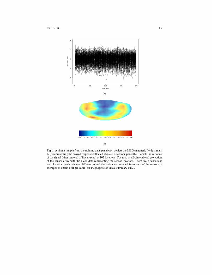
Our third and final objective is to illustrate these methods in a real applicationinvolving MEG data, where the goal is to explore variability in the brain data and touse the data to infer the type of video stimulus shown to a subject from a 1-secondrecording obtained from 204 MEG sensors with the signal at each channel sampledat a frequency of 200Hz. Each sample thus yields 204×200 = 40800 observationsof magnetic field measurements outside the head. The goal is to decode which offive possible video stimuli was shown to the subject during the recording from thesemeasurements. The data arising from a single sample are shown in Figure 1, wherepanel (a) depicts the brain signals recorded across all sensors during the 1-second

High-Dimensional Brain Decoding 3

recording, and panel (b) depicts the variance of the signal at each location. Frompanel (b) we see that in this particular sample the stimulus evoked activity in theregions associated with the temporal and occipital lobes of the brain. The entiredataset for the application includes a total of 1380 such samples (727 training; 653test) obtained from the same subject which together yield a dataset of roughly 6gigabytes in compressed format.

Functional principal component analysis (FPCA) is the extension of standardfinite-dimensional PCA to the setting where the response variables are functions,a setting referred to as functional data. For clarity, we note here that the use ofthe word ’functional’ in this context refers to functional data as just described, andis not to be confused with functional neuroimaging data which refers to imagingdata measuring the function of the brain. Given a sample of functional observations(e.g. brain signals) with each signal assumed a realization of a square-integrablestochastic process over a finite interval, FPCA involves the estimation of a set ofeigenvalue-eigenfunction pairs that describe the major vibrational components inthe data. These components can be used to define features for classification throughthe projection of each signal onto a set of estimated eigenfunctions characterizingmost of the variability in the data. This approach has been used recently for the clas-sification of genetic data by Leng and Muller (2005) who use FPCA in combinationwith logistic regression to develop a classifier for temporal gene expression data.

An alternative approach for exploring the patterns in brain signals is based onviewing each signal obtained at a voxel or sensor as a point in high-dimensional Eu-clidean space. The collection of signals across the brain then forms a point cloud inthis space, and the shape of this point cloud can be described using tools from topo-logical data analysis (Carlson, 2009). In this setting the data are assumed clusteredaround a familiar object like a manifold, algebraic variety or cell complex and theobjective is to describe (estimate some aspect of) the topology of this object fromthe data. The subject of persistent homology can be seen as a concrete manifesta-tion of this idea, and provides a novel method to discover non-linear features in data.With the same advances in modern computing technology that allow for the storageof large datasets, persistent homology and its variants can be implemented. Featuresderived from persistent homology have recently been found useful for classificationof hepatic lesions (Adcock et al., 2014) and persistent homology has been appliedfor the analysis of structural brain images (Chung et al., 2009; Pachauri et al., 2011).Outside the arena of medical applications, Sethares and Budney (2013) use persis-tent homology to study topological structures in musical data. Recent work in Heo etal. (2012) connects computational topology with the traditional analysis of varianceand combines these approaches for the analysis of multivariate orthodontic land-mark data derived from the maxillary complex. The use of persistent homology forexploring structure of spatiotemporal functional neuroimaging data does not appearto have been considered previously.

Another alternative for exploring patterns in the data is based on estimating andsummarizing the topology of an underlying network. Networks are commonly usedto explore patterns in both functional and structural neuroimaging data. With theformer, the nodes of the network correspond to the locations of sensors/voxels and


the links between nodes reflect some measure of dependence between the time se-ries collected at pairs of locations. To characterize dependence between time series,the mutual information, a measure of shared information between two time seriesis a useful quantity as it measures both linear and nonlinear dependence (Zhou etal., 2009), the latter being potentially important when characterizing dependencebetween brain signals (Stam et al., 2003). Given such a network, the correspond-ing topology can be summarized with a small number of meaningful measures suchas those representing the degree of small-world organization (Rubinov and Sporns,2010). These measures can then be explored to detect differences in the networkstructure of brain activity across differing stimuli and can be further used as fea-tures for brain decoding.

The remainder of the paper is structured as follows. Section 2 describes the classi-fier and discusses important considerations for defining features. Section 3 providesa review of FPCA from the perspective of exploring functional neuroimaging data.Sections 4 and 5 discuss persistent homology and mutual information networks,respectively, as approaches for characterizing the interaction of brain signals anddefining nonlinear features for classification. Section 6 presents an application tothe decoding of visual stimuli from MEG data, and Section 7 concludes with a briefdiscussion.

2 Decoding Cognitive States from Neuroimaging Data

Let us assume we have observed functional neuroimaging data Y = {yi(t), i =1, . . . ,n; t = 1, . . . ,T} where yi(t) denotes the signal of brain activity measuredat the ith sensor or voxel. We assume that there is a well-defined but unknowncognitive state corresponding to these data that can be represented by the labelC ∈ {1, . . . ,K}. The decoding problem is that of recovering C from Y . A solution tothis problem involves first summarizing Y through an m-dimensional vector of fea-tures Y f = (Yf1 , . . . ,Yfm)

′ and then applying a classification rule Rm→{1, . . . ,K} toobtain the predicted state. A solution must specify how to construct the features anddefine the classification rule, and we assume there exists a set of training samplesY l = {yli(t), i= 1, . . . ,n; t = 1, . . . ,T}, l = 1, . . . ,L with known labels Cl , l = 1, . . . ,Lfor doing this.

To define the classification rule we model the training labels with a multinomialdistribution where the class probabilities are related to features through a symmetricmultinomial logistic regression (Friedman et al., 2010) having form

Pr(C = j) =exp(β0 j +β ′jY f )

∑Kk=1 exp(β0k +β ′kY f )

, j = 1, . . . ,K (1)

with parameters θ = (β01,β′1, . . . ,β0K ,β

′K)′. As the dimension of the feature vec-

tor will be large relative to the number of training samples we estimate θ from thetraining data using regularized maximum likelihood. This involves maximizing a pe-


nalized log-likelihood where the likelihood is defined by the symmetric multinomiallogistic regression and we incorporate an elastic net penalty (Zou and Hastie, 2006).Optimization is carried using cyclical coordinate descent as implemented in the glm-net package (Friedman et al., 2010) in R. The two tuning parameters weighting thel1 and l2 components of the elastic net penalty are chosen using cross-validationover a grid of possible values. Given θ the classification of a new sample with un-known label is based on computing the estimated class probabilities from (1) andchoosing the state with the highest estimated value.

To define the feature vector Y f from Y we consider two aspects of the neuralsignal that are likely important for discriminating cognitive states. The first aspectinvolves the shape and power of the signal at each location. These are local featurescomputed at each voxel or sensor irrespective of the signal observed at other loca-tions. The variance of the signal computed over all time points is one such featurethat will often be useful for discriminating states, as different states may correspondto different locations of activation, and these locations will have higher variabilityin the signal. The second aspect is the functional connectivity representing how sig-nals at different locations interact. Rather than being location specific, such featuresare global and may help to resolve the cognitive state in the case where states cor-respond to differing patterns of interdependence among the signals across the brain.From this perspective we next briefly describe FPCA, persistent homology, and mu-tual information networks as approaches for exploring these aspects of functionalneuroimaging data, and further how these approaches can be used to define featuresfor classification.

3 Functional Principal Component Analysis

Let us fix a particular location i of the brain or sensor array. At this specific loca-tion we observe a sample of curves yli(t), l = 1, . . . ,L where the size of the samplecorresponds to that of the training set. We assume that each curve is an indepen-dent realization of a square-integrable stochastic process yi(t) on [0,T ] with meanE[yi(t)] = µi(t) and covariance Cov[yi(t),yi(s)] = Gi(s, t). The process can be writ-ten in terms of the Karhunen-Loeve representation (Leng and Muller, 2005)

yi(t) = µi(t)+∑m

εmiρmi(t) (2)

where {ρmi(t)} is a set of orthogonal functions referred to as the functional principalcomponents (FPCs) with corresponding coefficients

εmi =∫ T

0(yi(t)−µi(t))ρmi(t)dt (3)

with E[εmi] = 0, Var[εmi] = λmi and the variances are ordered so that λ1i ≥ λ2i ≥ ·· ·with ∑m λmi <∞. The total variability of process realizations about µi(t) is governed


by the random coefficients εmi and in particular by the corresponding variance λmi,with relatively higher values corresponding to FPCs that contribute more to this totalvariability.

Given the L sample realizations, the estimates of µi(t) and of the first few FPCscan be used to explore the dominant modes of variability in the observed brainsignals at location i. The mean curve is estimated simply as µi(t) = 1

L ∑Ll=1 yli(t)

and from this the covariance function Gi(s, t) is estimated Gi = ˆCov[yi(sk),yi(sl)]using the empirical covariance over a grid of points s1, . . . ,sS ∈ [0,T ]. The FPCsare then estimated through the spectral decomposition of Gi (see e.g. Ramsay andSilverman, 2005) with the eigenvectors yielding the estimated FPCs evaluated atthe grid points, ρ mi = (ρ mi(s1), . . . , ρ mi(sS))

′, and the corresponding eigenvaluesbeing the estimated variances λmi for the coefficients εmi in (2). The fraction of thesample variability explained by the first M estimated FPCs can then be expressed asFV E(M) = ∑

Mm=1 λmi/∑m λmi and this can be used to choose a nonnegative integer

Mi so that the predicted curves

yli(t) = µi(t)+Mi

∑m=1

εlmiρmi(t)

explain a specified fraction of the total sample variability. We note that in producingthe predicted curve a separate realization of the coefficients εmi from (2) is estimatedfrom each observed signal using (3) and, for a given m, the estimated coefficientsε mi = {εlmi, l = 1, . . . ,L} are referred to as the order-m FPC scores which representbetween subject variability in the particular mode of variation represented by ρmi(t).The scores are thus potentially useful as features for classification.

We compute the FPC scores ε mi, m = 1, . . . ,Mi separately at each location i =1, . . . ,n. For a given location the number of FPCs, Mi, is chosen to be the smallestinteger such that the FV E(Mi)≥ 0.9. Thus the number of FPCs, Mi, will vary acrosslocations but typically only a small number will be required. Locations requiringa relatively greater number of FPCs will likely correspond to locations where thesignal is more complex. The total number of features introduced by our applicationof FPCA for brain decoding is then ∑

ni=1 Mi. The FPCs and the associated FPC

scores are computed using the fda package in R (Ramsay and Silverman, 2005).

4 Persistent Homology

Let us now fix a particular sample l from the training set and consider the col-lection of signals, yli(t), observed over all locations i = 1, . . . ,n for that sam-ple. Each signal is observed over the same set of T equally-spaced time pointsY li = (yli(1), . . . ,yli(T ))′ and can thus be considered a point in RT . The sampleof signals across the brain/sensors then forms a point cloud in RT . For example, thesingle sample depicted in Figure 1, panel (a), represents a cloud of n = 204 pointsin R200. Using tools from topological data analysis we aim to identify topological


structures associated with this point cloud and to use such structures as features forbrain decoding.

As a metric inducing the topology we require a measure of statistical dependencethat will collate both correlated and anti-correlated signals. We therefore employ theabsolute Pearson correlation distance metric D(Y li,Y l j) = 1− ρ(Y li,Y l j)

2 whereρ(Y li,Y l j) is the sample correlation between signals at locations i and j. We focusspecifically on persistent homology, which attempts to identify the connected com-ponents, loops, and voids of an associated manifold that we assume the point cloudhas been sampled from. The general idea is to approximate the manifold using asimpler object, a simplicial complex, for which the homology (a characterization ofthe holes in the shape) may be calculated. A sequence of such approximations cov-ering a range of scales is considered and the features that persist over a large rangeare considered as intrinsic to the data. We provide here only a general descriptionthat emphasizes basic concepts and intuition for the construction of features forbrain decoding. A more detailed but still gentle introduction to persistent homologyincluding the required definitions and results from simplicial homology theory andgroup theory is provided by Zhu (2013).

Given the point cloud of n signals and the metric based on correlation distance,we consider a covering of the points by balls of radius ε , and for any such covering,we associate a simplicial complex for which the homology classes can be calcu-lated. The p-th Betti number, Bettip, can be thought of as representing the numberof p-dimensional holes, which for p = 0,1,2 corresponds to the number of con-nected components, loops and voids, respectively. The value of ε is then varied overmany possible values creating a filtration (an increasing sequence of simplicial com-plexes). The growing radius ε corresponds to allowing signals with smaller valuesof the squared-correlation to be linked together to form simplices in the simplicialcomplex. The homology classes are calculated at each value of ε to determine howthe system of holes changes. Persistent features remain over a relatively large rangeof ε values and are thus considered as signal in the data.

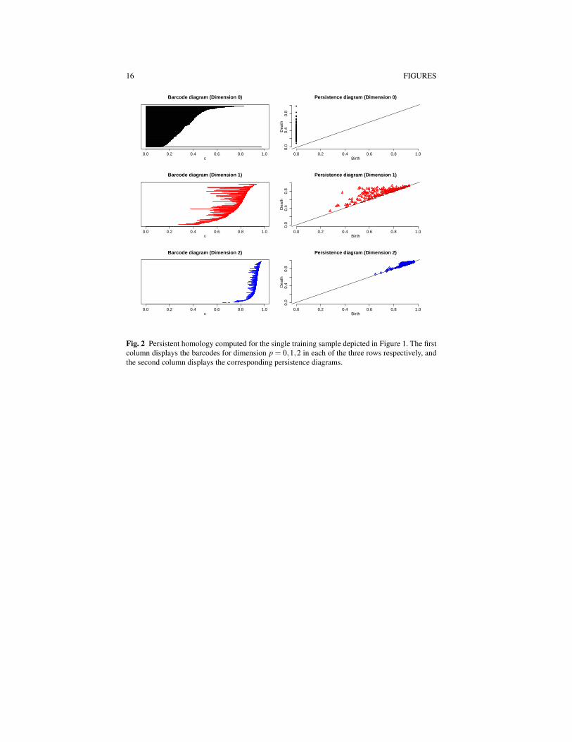
The nature of change with respect to each dimension p can be depicted graphi-cally using a barcode plot, a plot that tracks the birth and death of holes as ε varies.Features in the barcode that are born and then quickly die are considered topo-logical noise, while features that persist are considered indicative of signal in theunderlying topology. If the barcode plot of dimension p = 0 reveals signal and thehigher-dimensional barcodes do not, the data are clustered around a metric tree. Ifboth the p = 0 and p = 1 barcodes reveal signal and the p = 2 barcode plot does not,the data are clustered around a metric graph. A metric graph is indicative of multiplepathways for signals to get between two sensors/voxels. For barcodes of dimensionp > 1 the details can be rather subtle to sort through. For the sample consideredin Figure 1, panel (a), the barcodes for each dimension p = 0,1,2 are depicted inthe first column of Figure 2. For a given barcode plot, the Betti number for fixedε is computed as the number of bars above it. For p = 0 (Figure 2, first row andfirst column), Betti0 = 204 connected components are born at ε = 0 correspondingto each of the MEG sensors. Betti0 decreases rapidly as ε increases and it appearsthat between two to four connected components persist over a wide range of ε val-


ues. The barcode plot for dimension p = 1 (Figure 2, second row and first column)also appears to have features that are somewhat significant, but the p = 2 barcodesare relatively short, indicating noise. Taken together this can be interpreted as therebeing many loops in the point cloud. The data resemble a metric graph with somenoise added. An equivalent way to depict the persistence of features is through apersistence diagram, which is a scatter plot comparing the birth and death ε val-ues for each hole. The persistence diagrams corresponding to each barcode are aredepicted in the second column of Figure 2.

As for interpretation in the context of functional neuroimaging data, the numberof connected components (Betti0) represents a measure of the overall connectivityor synchronization between sensors, with smaller values of Betti0 corresponding toa greater degree of overall synchrony. We suspect that the number of loops (Betti1)corresponds to the density of ’information pathways’ with higher values correspond-ing to more complex structure having more pathways. The number of voids (Betti2)may be related to the degree of segregation of the connections. If a void was to per-sist through many values of ε , then we may have a collection of locations/sensorsthat are not communicating. Thus the larger the value of Betti2, the more of thesenon-communicative spaces there may be.

For each value of p, p = 0,1,2, we construct features for classification by ex-tracting information from the corresponding barcode by considering the persistenceof each hole appearing at some point in the barcode. This is defined as the differencebetween the corresponding death and birth ε values for a given hole. This yields asample of persistence values for each barcode. Summary statistics computed fromthis sample are then used as features for classification. In particular, we compute thetotal persistence, PMp, which is defined as one-half of the sum of all persistence val-ues, and we also compute the variance, skewness, and kurtosis of the sample leadingto additional features denoted as PVp, PSp, PKp, respectively. In total we obtain 12global features from persistent homology.

5 Mutual Information Networks

Let us again fix a particular sample l from the training set and consider the collec-tion of signals, yli(t), observed over all locations i = 1, . . . ,n for the given sam-ple. For the moment we will suppress dependence on training sample l and letY i = (Yi(1), . . . ,Yi(T ))′ denote the time series recorded at location i. We next con-sider a graph theoretic approach that aims to characterize the global connectivityin the brain with a small number of neurobiologically meaningful measures. Thisis achieved by estimating a weighted network from the time series where the sen-sors/voxels correspond to the nodes of the network and the links w = (wi j) representthe connectivity, where wi j is a measure of statistical dependence estimated from Y iand Y j.

As a measure of dependence we consider the mutual information which quan-tifies the shared information between two time series and measures both linear


and nonlinear dependence. The coherence between Y i and Y j at frequency λ is ameasure of correlation in frequency and is defined as cohi j(λ ) = | fi j(λ )|2/( fi(λ )∗f j(λ )) where fi j(λ ) is the cross-spectral density between Y i and Y j and fi(λ ), f j(λ )are the corresponding spectral densities for each process (see e.g. Shumway andStoffer, 2011). The mutual information within frequency band [λ1,λ2] is then

δi j =−1

2π

∫λ2

λ1

log(1− cohi j(λ ))dλ

and the network weights are defined as wi j =√

1− exp(−2δi j) which gives a mea-sure of dependence lying in the unit interval (Joe, 1989). The estimates w are basedon values λ1 = 0, λ2 = 0.5, and computed using the MATLAB toolbox for functionalconnectivity (Zhou et al., 2009). After computing the estimates of the network ma-trices we retained only the top 20% strongest connections and set the remainingweights to wi j = 0.

We summarize the topology of the network obtained from each sample withseven graph-theoretic measures, each of which can be expressed explicitly as afunction of w (see e.g. Rubinov and Sporns, 2010). In computing the measures,the distance between any two nodes is taken as w−1

i j :

1. Characteristic path length: the average shortest path between all pairs of nodes.2. Global efficiency: the average inverse shortest path length between all pairs of

nodes.3. Local efficiency: global efficiency computed over node neighbourhoods.4. Clustering coefficient: an average measure of the prevalence of clustered connec-

tivity around individual nodes.5. Transitivity: a robust variant of the clustering coefficient.6. Modularity: degree to which the network may be subdivided into clearly delin-

eated and non-overlapping groups.7. Assortativity coefficient: correlation coefficient between the degrees of all nodes

on two opposite ends of a link.

The seven measures are computed for each training sample and used as global fea-tures for brain decoding.

6 Example Application: Brain Decoding from MEG

In 2011 the International Conference on Artificial Neural Networks (ICANN) heldan MEG mind reading contest sponsored by the PASCAL2 Challenge Programme.The challenge task was to infer from brain activity, measured with MEG, the typeof a video stimulus shown to a subject. The experimental paradigm involved onemale subject who watched alternating video clips from five video types while MEGsignals were recorded at n = 204 sensor channels covering the scalp. The differentvideo types are:


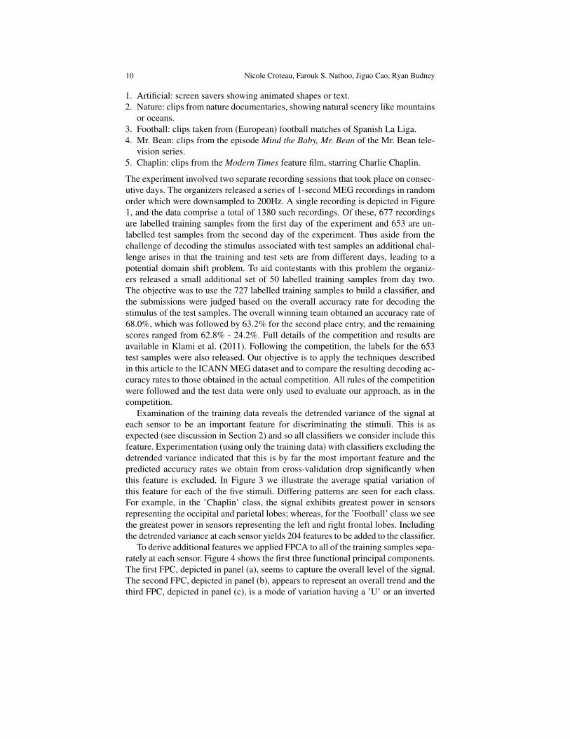
1. Artificial: screen savers showing animated shapes or text.2. Nature: clips from nature documentaries, showing natural scenery like mountains

or oceans.3. Football: clips taken from (European) football matches of Spanish La Liga.4. Mr. Bean: clips from the episode Mind the Baby, Mr. Bean of the Mr. Bean tele-

vision series.5. Chaplin: clips from the Modern Times feature film, starring Charlie Chaplin.

The experiment involved two separate recording sessions that took place on consec-utive days. The organizers released a series of 1-second MEG recordings in randomorder which were downsampled to 200Hz. A single recording is depicted in Figure1, and the data comprise a total of 1380 such recordings. Of these, 677 recordingsare labelled training samples from the first day of the experiment and 653 are un-labelled test samples from the second day of the experiment. Thus aside from thechallenge of decoding the stimulus associated with test samples an additional chal-lenge arises in that the training and test sets are from different days, leading to apotential domain shift problem. To aid contestants with this problem the organiz-ers released a small additional set of 50 labelled training samples from day two.The objective was to use the 727 labelled training samples to build a classifier, andthe submissions were judged based on the overall accuracy rate for decoding thestimulus of the test samples. The overall winning team obtained an accuracy rate of68.0%, which was followed by 63.2% for the second place entry, and the remainingscores ranged from 62.8% - 24.2%. Full details of the competition and results areavailable in Klami et al. (2011). Following the competition, the labels for the 653test samples were also released. Our objective is to apply the techniques describedin this article to the ICANN MEG dataset and to compare the resulting decoding ac-curacy rates to those obtained in the actual competition. All rules of the competitionwere followed and the test data were only used to evaluate our approach, as in thecompetition.

Examination of the training data reveals the detrended variance of the signal ateach sensor to be an important feature for discriminating the stimuli. This is asexpected (see discussion in Section 2) and so all classifiers we consider include thisfeature. Experimentation (using only the training data) with classifiers excluding thedetrended variance indicated that this is by far the most important feature and thepredicted accuracy rates we obtain from cross-validation drop significantly whenthis feature is excluded. In Figure 3 we illustrate the average spatial variation ofthis feature for each of the five stimuli. Differing patterns are seen for each class.For example, in the ’Chaplin’ class, the signal exhibits greatest power in sensorsrepresenting the occipital and parietal lobes; whereas, for the ’Football’ class we seethe greatest power in sensors representing the left and right frontal lobes. Includingthe detrended variance at each sensor yields 204 features to be added to the classifier.

To derive additional features we applied FPCA to all of the training samples sepa-rately at each sensor. Figure 4 shows the first three functional principal components.The first FPC, depicted in panel (a), seems to capture the overall level of the signal.The second FPC, depicted in panel (b), appears to represent an overall trend and thethird FPC, depicted in panel (c), is a mode of variation having a ’U’ or an inverted


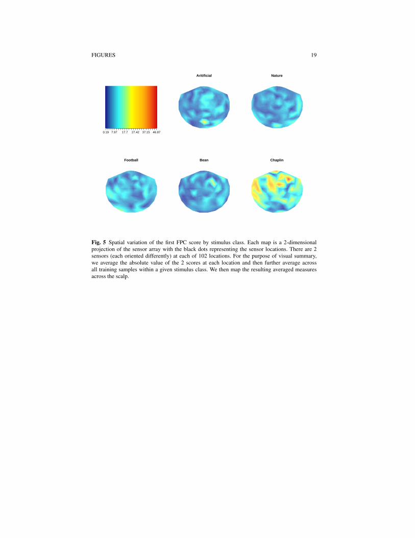
’U’ shape. At each sensor, we included as features the minimum number of FPCscores required to explain 90% of the variability at that sensor across the trainingsamples. The distribution of the number of scores used at each sensor is depicted inFigure 4, panel (d). At most sensors either Mi = 2 or Mi = 3 FPC scores are usedas features, and overall, FPCA introduces 452 features. The spatial variability of thefirst FPC score is depicted in Figure 5. Differing spatial patterns across all of thestimuli are visible, in particular for the ’Chaplin’ class, which tends to have elevatedfirst FPC scores at many sensors.

Persistent homology barcodes of dimension p = 0,1,2 were computed using theTDA package in R (Fasy et al., 2014) for all training samples and the 12 summaryfeatures PMp,PVp,PSp,PKp, p = 0,1,2 were extracted from the barcodes. To de-termine the potential usefulness for classification we compared the mean of each ofthese features across the five stimuli classes using one-way analysis of variance. Inmost cases the p-value corresponding to the null hypothesis of equality of the meanacross all groups was less than 0.05, with the exception of PK0 (p-value = .36) andPM1 (p-value = .34). Mutual information weighted networks were also computedfor each training sample and the seven graph theory measures discussed in Section5 were calculated. Analysis of variance comparing the mean of each graph mea-sure across stimuli classes resulted in p-values less than 0.001 for all seven features.This initial analysis indicates that both types of features, particularly the networkfeatures, may be useful for discriminating the stimuli for these data.

We considered a total of seven classifiers based on the setup described in Sec-tion 2 each differing with respect to the features included. The features included ineach of the classifiers are indicated in Table 1. The simplest classifier included onlythe detrended variance (204 features) and the most complex classifier included thedetrended variance, FPCA scores, persistent homology statistics, and graph theorymeasures (675 features). As discussed in Section 2, the regression parameters θ areestimated by maximizing the log-likelihood of the symmetric multinomial logisticregression subject to an elastic net penalty. The elastic net penalty is a mixture ofridge and lasso penalties and has two tuning parameters, λ ≥ 0 a complexity parame-ter, and 0≤α ≤ 1 a parameter balancing the ridge (α = 0) and lasso (α = 1) compo-nents. We choose values for these tuning parameters using cross-validation based ona nested cross-validation scheme similar to that proposed in Huttunen et al. (2011)that emphasizes the 50 labelled day two samples for obtaining error estimates. Weconsider a sequence of possible values for α lying in the set {0,0.1,0.2, . . . ,1.0}and fix α at one such value. With the given value of α fixed, we perform a 200-foldcross-validation. In each fold, the training data consists of all 677 samples from dayone and a random sample of 25 of the 50 labelled day two samples. The remaininglabelled day two samples are set aside as a validation set for the given fold. Withinthis fold, the 677+25 = 702 samples in the current training set are subjected to an-other 5-fold cross-validation over a sequence of λ values to obtain an optimal λ

value for the given α and training set. The resulting model is then used to classifythe 25 validation samples resulting in a performance estimate εα, j correspondingto the jth fold, j = 1, . . . ,200. The overall performance estimate for a given α isthen obtained as the mean over the 200 folds εα = 1

200 ∑200j=1 εα, j. This procedure is


repeated for all α in {0,0.1, ...,1.0}. The optimal value for the tuning parameter α

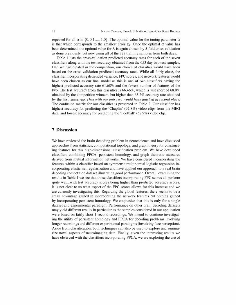
is that which corresponds to the smallest error εα . Once the optimal α value hasbeen determined, the optimal value for λ is again chosen by 5-fold cross-validationas done previously, but now using all of the 727 training samples from both days.

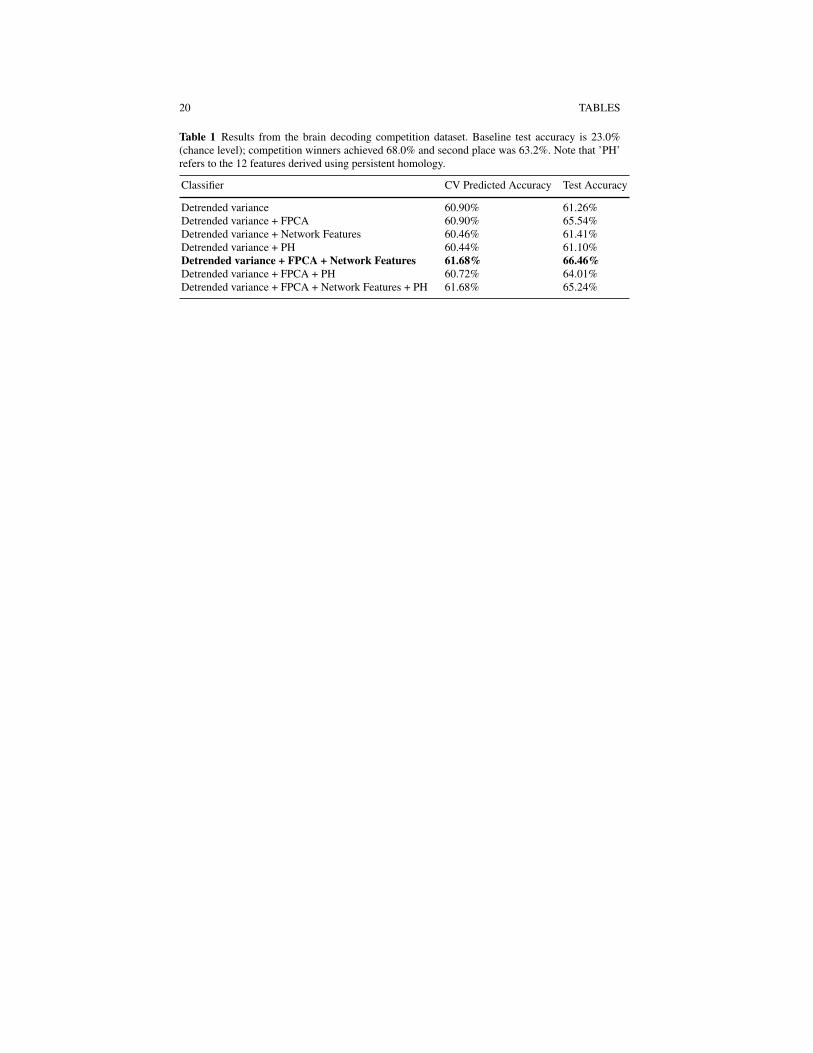
Table 1 lists the cross-validation predicted accuracy rates for each of the sevenclassifiers along with the test accuracy obtained from the 653 day two test samples.Had we participated in the competition, our choice of classifier would have beenbased on the cross-validation predicted accuracy rates. While all fairly close, theclassifier incorporating detrended variance, FPC scores, and network features wouldhave been chosen as our final model as this is one of two classifiers having thehighest predicted accuracy rate 61.68% and the fewest number of features of thetwo. The test accuracy from this classifier is 66.46%, which is just short of 68.0%obtained by the competition winners, but higher than 63.2% accuracy rate obtainedby the first runner-up. Thus with our entry we would have finished in second place.The confusion matrix for our classifier is presented in Table 2. Our classifier hashighest accuracy for predicting the ’Chaplin’ (92.8%) video clips from the MEGdata, and lowest accuracy for predicting the ’Football’ (52.9%) video clip.

7 Discussion

We have reviewed the brain decoding problem in neuroscience and have discussedapproaches from statistics, computational topology, and graph theory for construct-ing features for this high-dimensional classification problem. We have developedclassifiers combining FPCA, persistent homology, and graph theoretic measuresderived from mutual information networks. We have considered incorporating thefeatures within a classifier based on symmetric multinomial logistic regression in-corporating elastic net regularization and have applied our approach to a real braindecoding competition dataset illustrating good performance. Overall, examining theresults in Table 1 we see that those classifiers incorporating FPC scores all performquite well, with test accuracy scores being higher than predicted accuracy scores.It is not clear to us what aspect of the FPC scores allows for this increase and weare currently investigating this. Regarding the global features, there seems to be asmall advantage gained in incorporating the network features but nothing gainedby incorporating persistent homology. We emphasize that this is only for a singledataset and experimental paradigm. Performance on other brain decoding datasetsmay yield different results in particular as the samples considered in our applicationwere based on fairly short 1-second recordings. We intend to continue investigat-ing the utility of persistent homology and FPCA for decoding problems involvinglonger recordings and different experimental paradigms (involving face perception).Aside from classification, both techniques can also be used to explore and summa-rize novel aspects of neuroimaging data. Finally, given the interesting results wehave observed with the classifiers incorporating FPCA, we are exploring the use of


more general approaches based on nonlinear manifold representations for functionaldata such as those recently proposed by Chen and Muller (2012).

Acknowledgements This article is based on work from Nicole Croteau’s MSc thesis. F.S. Nathoois supported by an NSERC discovery grant and holds a Tier II Canada Research Chair in Biostatis-tics for Spatial and High-Dimensional Data.

References

1. Adcock, Aaron, Daniel Rubin, and Gunnar Carlsson. Classification of hepatic lesions usingthe matching metric. Computer vision and image understanding, 121, 36-42 (2014).

2. Carlsson, Gunnar. Topology and data. Bulletin of the American Mathematical Society, 46,255-308 (2009).

3. Chapelle, Olivier, Patrick Haffner, and Vladimir N. Vapnik. Support vector machines forhistogram-based image classification. Neural Networks, IEEE Transactions on, 10, 1055-1064 (1999).

4. Chen, Dong, and Hans-Georg Mller. Nonlinear manifold representations for functional data.The Annals of Statistics, 40, 1-29 (2012).

5. Chung, Moo K., Peter Bubenik, and Peter T. Kim. Persistence diagrams of cortical surfacedata. In Information Processing in Medical Imaging, 386-397. Springer Berlin, Heidelberg(2009).

6. Fasy, B. T., Kim, J., Lecci, F., and Maria, C. Introduction to the R package TDA. arXivpreprint arXiv:1411.1830. (2014).

7. Friedman, Jerome, Trevor Hastie, and Rob Tibshirani. Regularization paths for generalizedlinear models via coordinate descent. Journal of statistical software, 33, 1-22 (2010).

8. Friston, K., Chu, C., Mourao-Miranda, J., Hulme, O., Rees, G., Penny, W., and Ashburner, J.Bayesian decoding of brain images. Neuroimage, 39, 181-205 (2008).

9. Haynes, John-Dylan, and Geraint Rees. Decoding mental states from brain activity in humans.Nature Reviews Neuroscience 7, 523-534 (2006).

10. Heo, G., Gamble, J., and Kim, P. T. Topological Analysis of Variance and the MaxillaryComplex. Journal of the American Statistical Association,107, 477-492 (2012).

11. Huttunen, H., Manninen, T., Kauppi, J. P., and Tohka, J. Mind reading with regularized multi-nomial logistic regression. Machine vision and applications, 24, 1311-1325 (2013).

12. Joe, Harry. Relative entropy measures of multivariate dependence. Journal of the AmericanStatistical Association, 84, 157-164 (1989).

13. Klami, Arto, Ramkumar P., Virtanen S., Parkkonen L., Hari R., and Kaski, S.ICANN/PASCAL2 challenge: MEG mind readingoverview and results. Proceedings ofICANN/PASCAL2 Challenge: MEG Mind Reading (2011).

14. Leng, Xiaoyan, and Hans-Georg Muller. Classification using functional data analysis for tem-poral gene expression data. Bioinformatics, 22, 68-76 (2006).

15. Neal, Radford M., and Jianguo Zhang. High dimensional classification with Bayesian neuralnetworks and Dirichlet diffusion trees. Feature Extraction. Springer Berlin Heidelberg, 265-296 (2006).

16. Pachauri, Deepti, Chris Hinrichs, Moo K. Chung, Sterling C. Johnson, and Vikas Singh.Topology-Based Kernels With Application to Inference Problems in Alzheimer’s Disease.Medical Imaging, IEEE Transactions on, 30, 1760-1770 (2011).

17. Silverman, B. W., and J. O. Ramsay. Functional Data Analysis. Springer, (2005).18. Rasmussen, Carl Edward. Gaussian processes in machine learning. Advanced lectures on

machine learning. Springer Berlin Heidelberg, 63-71 (2004).19. Ripley, Brian D. Neural networks and related methods for classification. Journal of the Royal

Statistical Society. Series B (Methodological), 56, 409-456 (1994).


20. Rubinov, M., Sporns, O. Complex network measures of brain connectivity: uses and interpre-tations. Neuroimage, 52, 1059-1069 (2010).

21. Sethares, William A., and Ryan Budney. Topology of musical data. Journal of Mathematicsand Music 8, 73-92 (2014).

22. Shumway, Robert H., and David S. Stoffer. Spectral analysis and filtering. Time Series Anal-ysis and Its Applications. Springer New York, (2011).

23. Stam, C. J., Breakspear, M., van Walsum, A. M. V. C., and van Dijk, B. W. Nonlinear synchro-nization in EEG and whole?head MEG recordings of healthy subjects. Human brain mapping,19, 63-78 (2003).

24. Tomioka, Ryota, Kazuyuki Aihara, and Klaus-Robert Muller. Logistic regression for singletrial EEG classification. Advances in neural information processing systems, 19, 1377-1384(2007).

25. Zhou, Dongli, Wesley K. Thompson, and Greg Siegle. MATLAB toolbox for functional con-nectivity. Neuroimage, 47, 1590-1607 (2009).

26. Zhu, Xiaojin. Persistent homology: An introduction and a new text representation for naturallanguage processing. In Proceedings of the Twenty-Third international joint conference onArtificial Intelligence. AAAI Press, 2013.

27. Zou, Hui, and Trevor Hastie. Regularization and variable selection via the elastic net. Journalof the Royal Statistical Society: Series B (Statistical Methodology), 67, 301-320 (2005).

FIGURES 15

0 50 100 150 200

−4

−2

02

4

Time point

Obs

erve

d da

ta

(a)

0.08 0.11 0.14 0.17 0.2 0.23 0.26 0.29 0.32 0.35 0.38 0.41 0.44

(b)

Fig. 1 A single sample from the training data: panel (a) - depicts the MEG (magnetic field) signalsYli(t) representing the evoked response collected at n= 204 sensors; panel (b) - depicts the varianceof the signal (after removal of linear trend) at 102 locations. The map is a 2-dimensional projectionof the sensor array with the black dots representing the sensor locations. There are 2 sensors ateach location (each oriented differently) and the variance computed from each of the sensors isaveraged to obtain a single value (for the purpose of visual summary only).

16 FIGURES

Barcode diagram (Dimension 0)

0.0 0.2 0.4 0.6 0.8 1.0ε

Persistence diagram (Dimension 0)

0.0 0.2 0.4 0.6 0.8 1.0

0.0

0.4

0.8

Birth

Dea

th


0.0 0.2 0.4 0.6 0.8 1.0ε


0.0 0.2 0.4 0.6 0.8 1.0

0.0

0.4

0.8

Birth

Dea

th


0.0 0.2 0.4 0.6 0.8 1.0ε


0.0 0.2 0.4 0.6 0.8 1.0

0.0

0.4

0.8

Birth

Dea

th

Fig. 2 Persistent homology computed for the single training sample depicted in Figure 1. The firstcolumn displays the barcodes for dimension p = 0,1,2 in each of the three rows respectively, andthe second column displays the corresponding persistence diagrams.

FIGURES 17

0.11 0.2 0.3 0.4 0.49 0.59 0.68

Aritificial Nature

Football Bean Chaplin

Fig. 3 Spatial variation of the detrended variance by stimulus class. Each map is a 2-dimensionalprojection of the sensor array with the black dots representing the sensors. At each sensor we fit alinear regression on time point and compute the variance of the residuals as the feature. There are2 sensors (each oriented differently) at each of 102 locations. For the purpose of visual summary,we average the two variance measures for each location and then further average across all trainingsamples within a given stimulus class. We then map the resulting averaged measures across thescalp.

18 FIGURES

0 50 100 150 200

−0.

15−

0.10

−0.

050.

000.

050.

100.

15

First FPC

Time point

W(t

)

0 50 100 150 200

−0.

15−

0.10

−0.

050.

000.

050.

100.

15

Second FPC

Time point

W(t

)

(a) (b)

0 50 100 150 200

−0.

15−

0.10

−0.

050.

000.

050.

100.

15

Third FPC

Time point

W(t

)

1 2 3 4

Number of FPC Scores at Sensor

Fre

quen

cy

020

4060

8010

012

0

(c) (d)

Fig. 4 FPCA applied to the training data: panel (a) - the first FPC at each sensor; panel (b) - thesecond FPC at each sensor; panel (c) - the third FPC at each sensor; (d) - the distribution of thesmallest number of FPCs required to explain at least 90% of the variance at each sensor.

FIGURES 19

0.19 7.97 17.7 27.42 37.15 46.87

Aritificial Nature

Football Bean Chaplin

Fig. 5 Spatial variation of the first FPC score by stimulus class. Each map is a 2-dimensionalprojection of the sensor array with the black dots representing the sensor locations. There are 2sensors (each oriented differently) at each of 102 locations. For the purpose of visual summary,we average the absolute value of the 2 scores at each location and then further average acrossall training samples within a given stimulus class. We then map the resulting averaged measuresacross the scalp.

20 TABLES

Table 1 Results from the brain decoding competition dataset. Baseline test accuracy is 23.0%(chance level); competition winners achieved 68.0% and second place was 63.2%. Note that ’PH’refers to the 12 features derived using persistent homology.

Classifier CV Predicted Accuracy Test Accuracy

Detrended variance 60.90% 61.26%Detrended variance + FPCA 60.90% 65.54%Detrended variance + Network Features 60.46% 61.41%Detrended variance + PH 60.44% 61.10%Detrended variance + FPCA + Network Features 61.68% 66.46%Detrended variance + FPCA + PH 60.72% 64.01%Detrended variance + FPCA + Network Features + PH 61.68% 65.24%

TABLES 21

Table 2 Confusion matrix summarizing the performance on the test data for the classifier incor-porating detrended variance, FPCA, and network features.

Predicted Stimulus \\ True Stimulus Artificial Nature Football Mr. Bean ChaplinArtificial 90 27 28 6 3Nature 39 98 16 6 0Football 14 12 54 12 4Mr. Bean 5 11 4 76 2Chaplin 2 3 0 25 116

high-dimensional classification for brain decoding

Documents