high-speed railroad and economic geography: evidence … · adb economics working paper series...

ASIAN DEVELOPMENT BANK

AsiAn Development BAnk6 ADB Avenue, Mandaluyong City1550 Metro Manila, Philippineswww.adb.org

High-Speed Railroad and Economic Geography: Evidence from Japan

We study whether high-speed railroad (HSR) polarizes or balances economic geography using the 1982 opening of two major HSRs in Japan (Shinkansen). We find that both agglomeration and decentralization could occur. While service industry tends to agglomerate toward the core city, manufacturing industry may decentralize toward peripheral cities. We estimate that in noncore areas of Japan, service employment decreased by 7%, while manufacturing employment increased by 21%. Moreover, proximity between peripheral and core cities also matter. Cities within approximately 100 kilometers of Tokyo expanded, while more distant cities shrank. The net result is that Tokyo metropolitan area agglomerates because of HSR.

About the Asian Development Bank

ADB’s vision is an Asia and Pacific region free of poverty. Its mission is to help its developing member countries reduce poverty and improve the quality of life of their people. Despite the region’s many successes, it remains home to the majority of the world’s poor. ADB is committed to reducing poverty through inclusive economic growth, environmentally sustainable growth, and regional integration.

Based in Manila, ADB is owned by 67 members, including 48 from the region. Its main instruments for helping its developing member countries are policy dialogue, loans, equity investments, guarantees, grants, and technical assistance.

adb economicsworking paper series

NO. 485

may 2016

HiGH-SpEED RAilROAD AND EcONOmic GEOGRApHy: EviDENcE fROm JApANZhigang Li and Hangtian Xu

ADB Economics Working Paper Series

High-Speed Railroad and Economic Geography: Evidence from Japan Zhigang Li and Hangtian Xu

No. 485 | May 2016

Zhigang Li ([email protected]) is economist at the Economic Research and Cooperation Department, Asian Development Bank. Hangtian Xu ([email protected]) is assistant professor at the School of Economics and Trade, Hunan University, Changsha, People’s Republic of China. The authors thank Shangjin Wei, Zhiyuan Li, Kentaro Nakajima, Dao-Zhi Zeng, Ching-mu Chen, Tomoya Mori, Se-il Mun, Miwa Matsuo, Rana Hasan, and the participants of seminars at Asian Development Bank, Tohoku University, and Kyoto University for their comments. They are also grateful to Tetsuya Suzuki for the support in collecting the historical train timetables of Japan. This research was conducted when Hangtian Xu was a Japan Society for the Promotion of Science (JSPS) research fellow at Tohoku University. Professor Xu is also grateful for the financial support of JSPS (#26–4705).

Asian Development Bank 6 ADB Avenue, Mandaluyong City 1550 Metro Manila, Philippines www.adb.org

© 2016 by Asian Development Bank May 2016 ISSN 2313-6537 (Print), 2313-6545 (e-ISSN) Publication Stock No. WPS168070-2

The views expressed in this paper are those of the authors and do not necessarily reflect the views and policies of the Asian Development Bank (ADB) or its Board of Governors or the governments they represent.

ADB does not guarantee the accuracy of the data included in this publication and accepts no responsibility for any consequence of their use.

By making any designation of or reference to a particular territory or geographic area, or by using the term “country” in this document, ADB does not intend to make any judgments as to the legal or other status of any territory or area.

Note: In this publication, “$” refers to US dollars.

The ADB Economics Working Paper Series is a forum for stimulating discussion and eliciting feedback on ongoing and recently completed research and policy studies undertaken by the Asian Development Bank (ADB) staff, consultants, or resource persons. The series deals with key economic and development problems, particularly those facing the Asia and Pacific region; as well as conceptual, analytical, or methodological issues relating to project/program economic analysis, and statistical data and measurement. The series aims to enhance the knowledge on Asia’s development and policy challenges; strengthen analytical rigor and quality of ADB’s country partnership strategies, and its subregional and country operations; and improve the quality and availability of statistical data and development indicators for monitoring development effectiveness.

The ADB Economics Working Paper Series is a quick-disseminating, informal publication whose titles could subsequently be revised for publication as articles in professional journals or chapters in books. The series is maintained by the Economic Research and Regional Cooperation Department.

CONTENTS TABLES AND FIGURES iv ABSTRACT v I. INTRODUCTION 1 II. HYPOTHESES 5 III. EMPIRICAL SETTING 9 A. High-Speed Railroad Development in Japan 9 B. Macroeconomic Environment 13 IV. EMPIRICAL STRATEGY 15 A. Data 15 B. Empirical Specification 16 V. EMPIRICAL EVIDENCE 18 A. Agglomeration or Dispersion: Effect by Distance 18 B. Impact by Sector 23 C. Robustness Checks 24 VI. CONCLUSION 29 REFERENCES 31

TABLES AND FIGURES TABLES 1 High-Speed Railroads in Selected Economies 1 2 Employment Share by Industry in Japan, 1980–2005 14 3 Descriptive Summary of Dataset 16 4 Average Impact of TJL 18 5 Impact of TJL by Distance to Tokyo 21 6 Heterogeneity of the HSR Effects in Terms of Age 22 7 Impact of TJL by Service and Manufacturing Industries 24 8 Estimates with Alternative Control Groups 26 9 Control for the Effect of the National Highway 27 10 Baseline Results: Excluding Osaka 28 11 Robustness Check: Prefecture-Level Data 29 FIGURES 1 Total High-Speed Rail Mileage of the World 2 2 Japan High-Speed Rail Network 4 3 Spatial Effect of High-Speed Railroad (Equation 3) 8 4 Sampled Regions 10 5 Shortest Travel Time by Rail 11 6 Transport Mode Choice of Passengers in Japan, early 1990s 12 7 High-Speed Railroad Passenger Traffic 13 8 Population of Japan, 1960–2010 14 9 Population Growth in Treatment and Control Municipalities (TJL versus TL) 20 10 The Estimated Coefficients of Equations (R.1) and (R.2) with Different Sample Periods 22 11 Employment Growth in Treated and Control Municipalities (TJL versus TL) 23 12 Impact of Joetsu Line: Taking the Planned Hokuriku Line as the Control 25 13 Population Growth in Treatment and Control Municipalities (JL versus HL) 26

ABSTRACT This study addresses the debate on whether high-speed railroad (HSR) polarizes or balances economic geography. We find that both can occur: while the service sector tends to agglomerate, the manufacturing sector may decentralize; moreover, economic activities may agglomerate from distant areas to the core, while dispersing from the core toward its periphery at the same time. The service sector is crucial in this process because, unlike other land transport infrastructure, HSR mainly saves transport time for people, but not cargo. Incorporating this feature to the model of Ottaviano et al. (2002), we show that HSR can lead to either polarization or diffusion depending on sector and distance between cities. This is supported by empirical evidence from the 1982 opening of two major HSRs in Japan (Shinkansen), which saved intercity travel time by as much as half. We find that in noncore areas service employment decreased by 7%, while manufacturing employment increased by 21%; cities within approximately 100 kilometers of Tokyo expanded, while more distant cities shrank. In net, Tokyo metropolitan area agglomerates as a result of HSR. Keywords: economic corridor, high-speed rail, inclusive growth JEL codes: H54, O18, R12

“There is a big debate about the economic benefits of high-speed rail. Bizarrely it has been suggested that HS2 might disadvantage the regions by sucking more economic activity into the south-east than it

generates in the regions.”1

Lord Adonis, former Secretary of State for Transport, UK, 2011

I. INTRODUCTION Almost 4 decades after the first wave of high-speed rail (HSR) investment in advanced economies, a new wave of investment is taking place globally, especially in developing countries such as the People’s Republic of China (PRC), Russian Federation, and Brazil (Table 1). The total operating length of HSR networks globally has grown from 4,864 kilometers (km) in 2000 to 22,954 km by 2014, with 12,754 km under construction and another 18,841 km planned to be constructed before 2025 (Figure 1). The significant travel time saving greatly improves population mobility, which will likely have profound impact on economic geography. Due to limited research on HSR, there is still a lack of consensus regarding the spatial impacts of HSR investment. One major policy debate is on whether HSR can help the growth of lagging economies by improving their connection to core cities, which is commonly considered a major positive externality underlying government initiatives to support HSR development, e.g., in the United Kingdom (UK).

Table 1: High-Speed Railroads in Selected Economies

Economy Start Year Max. Operating

Speed (km/h) Mileage by2014 (km)

Mileage to Be Constructedby 2025 (km)

Japan 1964 320 2,664 958 France 1981 320 2,036 3,164 Italy 1981 300 923 346 Germany 1988 300 1,352 787 Spain 1992 300 2,515 3,010 United States 2000 240 362 777 Republic of Korea 2004 300 412 296 Taipei,China 2007 300 345 9 People’s Republic of China 2008 350 11,132 11,348 Turkey 2009 250 688 2,227 Russian Federation – – 0 3,150 Portugal – – 0 1,006 Sweden – – 0 750 Poland – – 0 712 Brazil – – 0 511

km/h = kilometer per hour. Source: US High Speed Rail Association. 2014. High Speed Lines in The World. http://www.uic.org/IMG/pdf/ 20140901_high_speed_lines_in_the_world.pdf

1 HS2 refers to a high-speed rail proposal in the UK which is under preparatory work. Expected to be completed by 2026–

2033, it is for a new, dedicated “Y”-shaped high-speed rail network, initially between London and the West Midlands (Phase I) and then with “legs” to Manchester and Leeds (Phase II) (House of Commons 2011).

2 | ADB Economics Working Paper Series No. 485

Figure 1: Total High-Speed Rail Mileage of the World

Note: Dashed line refers to the length under construction or planned. Source: US High Speed Rail Association. 2014. High Speed Lines in the World. http://www.uic.org/IMG/pdf/ 20140901_high_speed_lines_in_the_world.pdf

Compared with other land transport modes, a distinctive feature of HSR is reducing the travel

time for interregional passengers, but not for goods or for intraregional commuters. This feature has been rarely explored so far.2 To understand the spatial impact of HSR, we extend the model of Ottaviano, Tabuchi, and Thisse (2002) to account for the passenger time saving feature of HSR.3 This model implies that the impact of HSR on economic geography varies by sector and the distance between core and noncore cities. If the distance is long, HSR may make the service sector agglomerate toward the core area; in contrast, manufacturing sector may move out of the core city due to its rising urban costs (i.e., living and commuting costs). If the distance between core and noncore cities is short, the service sector may decentralize toward the noncore city. These implications are consistent with patterns scattered in the empirical literature, although systematic econometric evidence testing them is highly limited.4 Below, we first summarize our empirical strategy and findings, we then compare them with the empirical literature.

2 Existing theories analyzing the spatial impact of transport costs largely focus on the manufacturing sector (trade theory)

and on the location choices of residents (urban theory), and these are motivated by traditional transport modes, especially trains and automobiles. Trade theory typically suggests that lower transport costs may lead to agglomeration (Krugman 1991; Fujita, Krugman, and Venables 1999), while urban theory often finds a decentralization effect within transport cost reduction, such as the monocentric urban models of Alonso (1964) and Fujita (1989). More recent theoretical studies have jointly considered both within-region commuting costs (for passengers) and interregional transport cost (for goods), such as Tabuchi (1998), Murata and Thisse (2005), and Tabuchi and Thisse (2006). In these models, the decrease in both within-region and interregional transport costs tends to induce agglomeration across regions. A series of empirical studies provide evidence on both theories (Baum-Snow 2007, Baum-Snow et al. 2014, Faber 2014).

3 Note that this HSR model may not apply to expressways. Although expressway is similar to HSR networks in significantly reducing the time costs for passengers, it is also a major transport mode for goods.

4 By describing the time patterns of various economic indicators, Chen and Hall (2011) examined the effect of HSRs on jurisdictions with different distances to London, and they also examine the impact on the service sector.

0

10,000

20,000

30,000

40,000

50,000

60,000

1960 1970 1980 1990 2000 2010 2020

Kilo

met

er

High-Speed Railroad and Economic Geography: Evidence from Japan | 3

We provide empirical evidence using data from Japan. Japan was the first country to build HSR, completing the Tokaido line in 1964 to connect Tokyo and the major cities to its south.5 In 1982, two new HSRs, Tohoku and Joetsu lines (TJL), were completed to connect Tokyo and a number of major cities to its north and northwest (Figure 2). This development process of HSR provides a quasi-experimental setting to identify the causal effect of HSR on the economy. Studying Japan’s HSR networks has several additional advantages. First, given the relatively small geographical scope of Japan (comparable with the size of Germany, but with only 11% of area developable), the three HSR lines cover the majority of the Japanese population. Hence, population flows into and out of our sample area should be limited, simplifying the empirical analysis. Second, despite its relatively small geographical scope, the population and number of municipalities of Japan are large (127 million population and more than 3,000 municipalities nationwide), thereby offering a sufficiently large number of observations for econometric estimation. Third, as our sample period (1980–2003) is after the “golden era” of Japan and no major reform events occurred, the confounding effects of simultaneous economic cycles are mitigated.6 Fourth, high-quality data on the population and employment in Japan are available at prefecture or municipality levels before and after the construction of HSRs in 1982.

We apply a standard difference-in-difference (DID) estimation on the panel dataset of Japan on population and employment, which are disaggregated at the municipality and sector levels. In our baseline exercise, the treatment group includes municipalities along the TJL in northern Japan, while the control group includes those along the Tokaido line (TL), which is in southern Japan. In our augmented model, we test the nonlinear distance effect of HSR on agglomeration/dispersion by allowing the effect to differ by between noncore municipalities and Tokyo. In addition, we also test the theoretical implication that HSR has differential impact on service and manufacturing sectors. Our findings strongly support theoretical implications. Specifically, we find that the establishment of HSR in Japan has induced a significant agglomeration in the service sector toward the Tokyo metropolitan area (MA) as well as its peripheral area (within approximately 30 minutes of core Tokyo via HSR). In contrast, the manufacturing sector diffused toward more distant noncore areas. In net, Tokyo MA population increased by as much as 10.5% due to the TJL. Moreover, the estimated impact of HSR is significant for working-age population, but insignificant for the youth and aged population. 5 For example, the one-way trip of 550 km between Tokyo and Osaka requires more than 7 hours by expressway or regular

train. In contrast, it takes 2.5 hours by HSR. 6 The annual gross domestic product (GDP) growth of Japan (at constant prices) reached more than 8% during the period

of 1955–1980 (the post-World War II “golden era”). It slowed down to less than 4% in the following 2 decades (Japan Statistical Yearbook).


Figure 2: Japan High-Speed Rail Network

(a) 1980 (b) 1982

(c) 2003

Source: Constructed by the authors.


Our findings are qualitatively consistent with a number of studies on HSRs in Europe, the PRC and Japan, even though they provide seemingly contradictory findings.7 Some studies, such as Qin (2014), find that noncore jurisdictions are weakened by HSR, while some others, such as Ahlfeldt and Feddersen (2010), find the reverse. They may be reconciled when we account for the distances between the noncore jurisdictions and core cities: when they are close, HSRs may lead to diffusion; when they are far away, HSRs can lead to agglomeration. For example, the German HSR studied by Ahlfeldt and Feddersen (2010) is approximately 200 km (Frankfurt–Cologne HSR), while the studies on Japan and the PRC are commonly above 500 km.8 Besides distance, service sector is also understudied in the literature. Some descriptive studies, including Chen and Hall (2011, 2012) and Murakami and Cervero (2012), examine the service sector and find evidence for the agglomeration of knowledge-intensive service in major node cities of HSR. Nevertheless, they do not study the spatial reallocation of service sector due to HSR.

The rest of this paper is organized as follows. In section II, we present our hypotheses based on a theoretical framework. Section III describes the economic background in Japan. Section IV presents the empirical strategy and describes the dataset. Section V reports the baseline results and robustness checks. Section VI concludes.

II. HYPOTHESES Regarding the spatial impact of HSRs, the empirical literature has documented a series of patterns on agglomeration or diffusion. The majority of studies, though, are based on models that focus on the reduction of cargo transport costs or of workers’ commuting time. In this study we emphasize a distinctive feature of HSR: it mainly affect passengers who travel between cities but not for daily commuting. The key implication we draw from this feature is that HSR can help people to travel across regions to consume services. Incorporating this to the model of Ottaviano, Tabuchi, and Thisse (2002) leads to the following testable hypothesis:

7 There are extensive studies on how traditional transport infrastructure affects economic geography. On the one hand,

Baum-Snow (2007) provides evidence on the decentralization of the population from the central cities of metropolitan statistical areas in the United States after the opening of interstate highways. Baum-Snow (2014) further exploits the different impacts of decentralization on residents and employment and on sectors. By focusing on manufacturing, Rothenberg (2011) finds that manufacturing activities have relocated along the new highways next to existing urban centers in Indonesia. On the other hand, some evidence supports the agglomeration effect of transport infrastructure. For example, Tang (2014) and Faber (2014) find that manufacturing firms tend to agglomerate in large markets after the creation of new transport infrastructures in Japan and the PRC, respectively.

8 Econometric studies on the effect of Shinkansen on the distribution of economic activities in Japan are rare. Sasaki, Ohashi, and Ando (1997) use simulation analysis to show that HSR will not necessarily contribute to regional dispersion. Mori (2012) observes that as the Tokaido line halved the Osaka–Tokyo travel time from 8 hours to 4 hours in 1964, the size of Tokyo relative to that of Osaka increased from 2.0 times in 1964 to 2.7 times in 2005. Case studies in Okada (1994) show that service industries such as tourism, conferences, and exhibitions benefit significantly from nearby HSR stations.


Hypothesis. If the distance between the core and the noncore cities is sufficiently long, transport cost reduction for passengers makes the service sector with increasing returns to scale (IRS) agglomerate toward the core city. If the distance is sufficiently short, the cost reduction for passengers makes the service sector with IRS diffuse toward the noncore city. In contrast, the spatial redistribution of manufacturing sector shows a contrasting pattern.

Patterns consistent with this hypothesis scattered in existing empirical literature, although they have not been examined systematically. An alternative model on HSR is discussed in Ahlfeldt and Feddersen (2010), which also pay explicit attention to the propassenger feature of HSR. This study focuses on the manufacturing sector, though, and the argument is that HSRs may also affect the marketing and distribution costs of manufactured goods. Moreover, Ahlfeldt and Feddersen (2010) allow HSRs to affect the commuting costs of residents. In our model, we explicitly assume that HSRs do not affect the commuting costs, which is the case in Japan (see section III for details).9 As we are essentially using the model of Ottaviano, Tabuchi, and Thisse (2002) and just give it a new interpretation, we do not repeat the full model here. Below, we summarize major features of the model, as well as key results that are relevant to our empirical work. Two-Sector Model The economy consists of two regions, H and F. There are farmers as well as workers. Farmers are evenly distributed across regions and spatially immobile. Workers are mobile between the two regions, and their share in region H is . The economy produces and consumes only two goods. One good (food) is homogeneous and tradable without trade costs. It is produced by farmers under constant returns to scale and perfect competition. We treat it as the numéraire of the economy. The second good (services) is nontradable, horizontally differentiated, and produced by workers under IRS and imperfect competition. Although services are not tradable, people can travel across regional boundaries to consume services. Here we assume that each individual consumes only one service variety on his/her trip to the other region and that the travel cost is .10 In equilibrium, each individual consumes all varieties of the service goods. His/her budget consists of the wage income and a fixed endowment. As there is a one-to-one relationship between firms and varieties in the economy, the number of firms is the number of varieties. Each firm sets its price to maximize its profit. The model assumes identical preferences across individuals represented by a quasi-linear utility function with a quadratic subutility:

9 The model of Bernard, Moxnes, and Saito (2015) also takes into account the feature that HSRs mainly affect the transport

of people but not goods. The focus of Bernard, Moxnes, and Saito (2015) is specifically on the spatial distribution of suppliers of intermediate goods.

10 In Ottaviano, Tabuchi, and Thisse (2002), the second good is a manufactured good, which can be traded at an additive cost of τ per unit of the good transported from one region to the other. Given our assumption for interregional consumption of service, our case is mathematically the same as that in Ottaviano, Tabuchi, and Thisse (2002). Moreover, we follow the original model to assume that service providers can charge different prices on local and nonlocal customers. An example of this is that, in Japan, people who live outside of Tokyo MA can enjoy discounted ticket prices for Tokyo’s Disneyland Park by purchasing travel package including accommodation, Disneyland ticket, and high-speed rail ticket.


0

2

0

2

000 )(2

)(2

)(),0 ),(;( qdiiqdiiqdiiqNiiqqUNNN

, (1)

where )(iq is the quantity of variety Ni ,0 , and 0q the quantity of the numéraire. N is the number of varieties. The parameters are such that 0 and 0 . With the price and consumption determined, firms’ profits and workers’ wage levels are pinned down.

In this model transport cost is a key determinant of the consumption of service goods as well as the size of the regional economy in equilibrium. Without urban costs, it can be shown that the economy agglomerates when interregional transport costs become sufficiently low.11 As shown in Equation (2), * corresponds to the threshold of transport cost and determines whether dispersion or agglomeration exist in equilibrium. Without loss of generality, assume that region H was originally greater than F, i.e., 1/2 . We refer to H as the core area. When transport cost is higher than * , cross-regional consumption of service goods is insufficient to sustain agglomeration at the city region. People would migrate from the core region H to the noncore region F, resulting in dispersion ( 1/2 ) in equilibrium. In contrast, when is less than * , firms in the core region enjoy higher profit than the noncore region due to the large size of the core region. Hence, the economy agglomerates toward H:

*

*

dispersion ( =1/2) Equilibrium

agglomeration ( =1)

. (2)

When urban costs are incorporated to the model, the effect of transport cost is more

complicated:

Equilibrium

dispersion ( 1/ 2) 2*

agglomeration ( 1) 1*

2*

dispersion ( 1/ 2) 1*

. (3)

Here, 1

*, 2* (0, *) . It suggests that dispersion is also possible when transport cost is low.

The intuition is the following: when interregional passenger travel cost decreases relatively to the commuting cost and land rent in the core city, it becomes more attractive for workers to live and work in “cheaper” noncore area and travel to the core area for service needs. This leads to a rise of interregional service trade.

11 This is proved in the Proposition 1 of Ottaviano, Tabuchi, and Thisse (2002).


Figure 3: Spatial Effect of High-Speed Railroad (Equation 3)

Sources: Ottaviano,Tabuchi, and Thisse 2002; Authors’ calculation and construction.

Three-Sector Model It is desirable to have manufacturing industry in the model in addition to service industry as manufacturing industry is typically sizable in an economy. Even though an HSR does not directly affect the transport costs of manufactured goods, there may be an indirect effect. For example, changing urban costs in the core area may crowd out manufacturing industries. As shown by Tabuchi and Thisse (2006), however, adding one more industry to the current model significantly complicates the analysis. This is mainly because HSR not only affects the urban cost in each area, but also changes the relative size of service and manufacturing industries through intersector migration of workers. This may result in multiple equilibria. To address this issue, Tabuchi and Thisse (2006) consider several special cases, one of which is particularly relevant in our case. Below we present this case.

The utility function now includes products from all three industries (agriculture, manufacturing, and service). The specification of the utility function encapsulates both the preference for diversity between the service and manufacturing industries, and a preference for variety of goods within each sector. As workers can choose which industry to work in, the size of an industry is now


endogenous, depending on the sectoral mobility of workers. Given the setup of Tabuchi and Thisse (2006), wages are equalized across regions.

Consider a special case in which the transport cost is positive for the service industry, but is zero for the manufacturing industry. This simplifies the problem as the price of a manufactured good is equal in the two regions. Given the higher urban costs in the core area, it is clearly more beneficial for manufacturers to move from the core area to the noncore area. It can be shown that the unique stable equilibrium for a certain range of commuting cost is that the service industry (industry 2 in their case) is fully concentrated in the core area, while the manufacturing industry (industry 1 in their case) exists in both regions.12

III. EMPIRICAL SETTING Our quasi-experimental exercise critically depends on the development timing of the HSR network in Japan, which we detail in this section. Moreover, we also examine the macroeconomic environment, including the evolution of industry structure and population dynamics, which are potential confounding factors. A. High-Speed Railroad Development in Japan Japan has 47 prefecture-level jurisdictions and more than 3,000 municipalities during most of our sample period.13 Its capital city, Tokyo, is located near the country’s geographic center and close to the east coast. Tokyo and 33 other prefectures are located in Honshu, the largest and most populous island of Japan (Figure 4). With a length of 1,300 km and width not more than 230 km, Honshu’s population in 2014 was 103 million, approximately 80% of Japan’s total population.

12 Proposition 3 of Tabuchi and Thisse (2006). 13 This refers to our study period during 1980–2003. After 2003, the number of municipality-level jurisdictions greatly

decreased because of mergers.


Figure 4: Sampled Regions

Notes: Prefectures connected by Tohoku and Joetsu lines (TJL) are Tochigi, Niigata, Gunma, Fukushima, Miyagi, Iwate, Aomori; Prefectures connected by Tokaido line (TL) are Shizuoka, Aichi, Gifu, Shiga, Kyoto, Osaka. Source: Constructed by the authors.

There was no plan for HSR network development until after the success of the first HSR, the

Tokaido line, which was completed in 1964 to connect Tokyo and the second largest city, Osaka, 515 km south of the capital. The Tokaido line halved the travel time between these two cities from 8 hours on a conventional train to 4 hours. The travel time was further shortened to 2.5 hours by 1992 due to improved HSR technology (Figure 5). Although the Tokaido line was controversial, it turned out to be highly successfully financially. The first 3 months alone witnessed 11 million passengers (Japan Times 1965). Despite the high profitability, the fare of Tokaido line is reasonable considering the dramatic saving of time. In 2009, a one-way ticket between Tokyo and Osaka was ¥14,000 (approximately $155) by Shinkansen and ¥8,500 ($94) by conventional train.14

14 For the evolution of railway fares, see http://www6.plala.or.jp/orchidplace/fare_tokyo_osaka.html (in Japanese).


Figure 5: Shortest Travel Time by Rail

km = kilometer. Source: Authors’ computations based on Miyawaki (1998), Shozawa (2011) and Shinkansen Time Table in 2001. Tokyo–Osaka: Tokaido line; Tokyo–Morioka: Tohoku line; Tokyo–Niigata: Joetsu line.

With the success of the Tokaido line, on March 1965 a plan to extend Tokaido line toward

southern Japan through Sanyo line was unveiled (Japan Times 1965). The construction of Sanyo line began in 1967 and its commercial service started from 1972. A more ambitious nationwide HSR network plan was announced in 1967, including two major lines, Tohoku and Joetsu lines, which connect Tokyo with major cities in northwestern and northern Japan, respectively (Japan Times 1967).15 Ministerial approval for these two lines came through on January 1971 (Leclerc 2002), and the construction began several months later (Japan Times 1971). For the major parts of the lines, Omiya–Niigata (Joetsu line) and Omiya–Morioka (Tohoku line), commercial service began in 1982. Measured by traffic volume, HSR has become the favorite transport mode in Japan for a distance range of 400–1,000 km (Figure 6). 15 The cost of constructing the HSR (Shinkansen) was raised in the form of government loans, railway bonds, and low-

interest loans from the World Bank (Smith 2003).

0

50

100

150

200

250

300

350

400

450

1980 1983 1986 1989 1992 1995 1998 2001Tokyo–Osaka (515 km) Tokyo–Morioka (497 km)Tokyo–Niigata (301 km)

Trav

el ti

me

in m

inut

es


Figure 6: Transport Mode Choice of Passengers in Japan, early 1990s

Source: Okada, H. 1994. Features and Economic and Social Effects of the Shinkansen. Japan Railway and Transport Review. 10. pp. 9–16.

In contrast to the rapid development in HSR network, conventional railroads in Japan,

especially railroad lines in our sample regions (Tohoku main line, Shin-etsu main line, Joetsu line, and Tokaido main line), have seen little additional investment after the 1960s. Moreover, highway investment was also slow during our study period. The highway length in the study regions increased from 11,776 to 16,217 km from 1980 to 2003 (with an annual growth rate of 1.4%).16

Our empirical exercises focus on the Tokaido, Tohoku, and Joetsu lines (the Sanyo and Hokuriku lines will be examined as additional control group in the robustness check). These three lines share a common end city in Tokyo, which is the core area of Japan. They accounted for 69% of Japan’s HSR network in 1982 and 75%–80% of the HSR passenger traffic of Japan during 1980–2003 (Figure 7). The Tokaido line covers seven prefectures in southern Honshu (not including Tokyo). By 1980, passenger traffic on this line has stabilized at around 83 million people per year. The Joetsu line (270 km) covers three prefectures, while the Tohoku line (466 km) covers six.17 These two lines carried over 100 million passengers annually by 2000 (Figure 7). Although some new HSR lines were completed in the 3 decades following 1982, they were short distance routes, accounting for less than 6% of total HSR traffic.

16 Source: Authors’ calculation based on official statistics of Japan. The study area refers to 13 prefectures as mentioned in

section IV.B. 17 The Joetsu line was further extended to 301 km in 1985. The Tohoku line was further extended to 497 km in 1985, 593 km

in 2002, and 675 km in 2010.

0

100

80

60

40

20

0200 400 600

kilometer

%

800 1,000 1,200


Figure 7: High-Speed Railroad Passenger Traffic

Source: Authors’ computation based on Japan High Speed Rail Passenger Traffic Statistics 2010.

The high population density and simple spatial structure of the HSR network in Japan provide

a favorable empirical setting to test the economic impact of HSR. The cities along the southern lines (Tokaido line) offer a natural control group, while those along the northern part (Joetsu and Tohoku lines) are the treatment group. The geographic scope of Japan conforms well with the competitiveness range of HSR: with Tokyo in the middle of Honshu, the majority of cities are within 600 km of Tokyo. Also importantly, Tokyo MA, including four prefectures Tokyo, Kanagawa, Chiba, and Saitama, is the largest MA of Japan, with population accounting for 24.5% of Japan’s population in 1980 and 27.8% by 2010 (Japan Statistical Yearbook).18 This gives us a mono-center setting, which helps test the implication of the model. B. Macroeconomic Environment In this section, we examine macroeconomic factors that could confound our empirical estimates, including economic cycles, spatial population movement due to non-HSR factors, and the evolving economic structure. After the Second World War, the annual growth domestic product (GDP) of Japan first grew rapidly, averaging 10% during 1961–1970, but then moderated to less than 5% between 1971 and 1990 (Japan Statistics Bureau). During 1985–1990, commercial land prices in large cities surged by 400%, but dropped abruptly and sharply in 1991 and fell by 80% in total in the following decade (Japan Real Estate Institute).19 After 1991, the economic growth of Japan stagnated, with annual GDP growth averaging around 1%. The economic structure of Japan shifted gradually toward service during the study period. The employment share of agriculture, forestry, and manufacturing 18 The second largest MA is Kyoto–Osaka–Kobe MA (14.8% share of the total population in 1980, and down to 14.4% in

2010, including four prefectures Kyoto, Osaka, Hyogo, and Nara). 19 Fluctuations in residential land prices were less strong but still remarkable.

0

20

40

60

80

100

120

140

160

1970 1980 1990 2000 2008Tokaido line Tohoku, Joetsu linesRest of the lines

Mill

ion

pers

ons


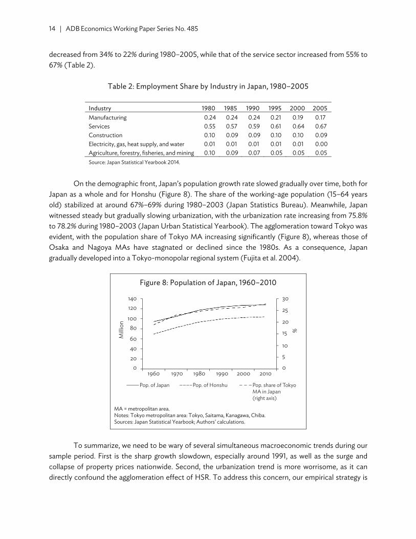
decreased from 34% to 22% during 1980–2005, while that of the service sector increased from 55% to 67% (Table 2).

Table 2: Employment Share by Industry in Japan, 1980–2005

Industry 1980 1985 1990 1995 2000 2005 Manufacturing 0.24 0.24 0.24 0.21 0.19 0.17 Services 0.55 0.57 0.59 0.61 0.64 0.67 Construction 0.10 0.09 0.09 0.10 0.10 0.09 Electricity, gas, heat supply, and water 0.01 0.01 0.01 0.01 0.01 0.00 Agriculture, forestry, fisheries, and mining 0.10 0.09 0.07 0.05 0.05 0.05 Source: Japan Statistical Yearbook 2014.

On the demographic front, Japan’s population growth rate slowed gradually over time, both for Japan as a whole and for Honshu (Figure 8). The share of the working-age population (15–64 years old) stabilized at around 67%–69% during 1980–2003 (Japan Statistics Bureau). Meanwhile, Japan witnessed steady but gradually slowing urbanization, with the urbanization rate increasing from 75.8% to 78.2% during 1980–2003 (Japan Urban Statistical Yearbook). The agglomeration toward Tokyo was evident, with the population share of Tokyo MA increasing significantly (Figure 8), whereas those of Osaka and Nagoya MAs have stagnated or declined since the 1980s. As a consequence, Japan gradually developed into a Tokyo-monopolar regional system (Fujita et al. 2004).

Figure 8: Population of Japan, 1960–2010

MA = metropolitan area. Notes: Tokyo metropolitan area: Tokyo, Saitama, Kanagawa, Chiba. Sources: Japan Statistical Yearbook; Authors’ calculations.

To summarize, we need to be wary of several simultaneous macroeconomic trends during our

sample period. First is the sharp growth slowdown, especially around 1991, as well as the surge and collapse of property prices nationwide. Second, the urbanization trend is more worrisome, as it can directly confound the agglomeration effect of HSR. To address this concern, our empirical strategy is

140

1960 1970 1980 1990 2000 2010

30

25

20

15 %

10

5

0

120

10080

60Milli

on

4020

0

Pop. of Japan Pop. of Honshu Pop. share of TokyoMA in Japan(right axis)


to use the DID estimation method, which is detailed in the following section. Moreover, we shall also conduct a number of robustness checks, including estimation using alternative control groups and different subsample periods, as well as controlling for pre-existing trends.

IV. EMPIRICAL STRATEGY Utilizing the empirical setting of Japan and its comprehensive data on demographics and employment, we propose to test the theoretical implications in section II with a DID methodology. We first present the dataset, and then discuss in detail our model specification and identification strategy. A. Data Our database is compiled from several sources. It includes annual residential population from 1980 to 2003 at the municipality level, from 1950 to 2003 at the prefecture level, and employment from 1980 to 2000 at a 5-year frequency at the municipality level.20 In addition, we also obtain information on the longitude and latitude information of municipalities to calculate their geographic distances to central Tokyo.21 The timing of HSR construction and operation, as well as the location of HSR stations, are based on publicly available reports.

As discussed in section III, our main regression sample covers 13 prefectures. The treatment group includes seven prefectures along TJL, namely Tochigi, Fukushima, Miyagi, Iwate, Aomori, Gunma, and Niigata, consisting of 515 municipalities in total. Our control group includes six prefectures along the Tokaido line, namely Shizuoka, Gifu, Shiga, Aichi, Osaka, and Kyoto, including 450 municipalities altogether. Table 3 provides summary statistics on the main variables. Jurisdictions along TJL are similar to those along Tokaido line in terms of average distance to Tokyo. In terms of local population and employment sizes, those along Tokaido line are larger than the treatment group on average. Population has grown slowly in the control group, while shrinking modestly in the treatment group. The pattern of change in industrial structure conforms well with the theoretical implication: in jurisdictions along TJL, the growth in service employment is slower but the growth in manufacturing employment is higher than in the control group. In fact, manufacturing employment in the control group shrunk during 1980–2003, while that in the treatment group grew.

20 Municipalities are identified by the five-digit administrative division code. Japan imposed a policy called the Great Heisei

Mergers (heisei-no-daigappei) in 1999 to merge the municipalities and decrease the number of municipality. Nevertheless, large-scale mergers did not start until 2004. During 1999–2003, the number of municipalities remained stable (3,232 in 1999 and 3,212 in 2003).

21 Data of residential population are from Residential Population Survey conducted by Local Administration Bureau, Ministry of Internal Affairs and Communications annually from 1980–2003. Data on employment by industry are from Population Census of Japan by Statistics Bureau, Ministry of Internal Affairs and Communications. Longitude and latitude data for each municipality are obtained from the Center for Spatial Information Science, The University of Tokyo (CSV Address Matching Service), by which we calculate municipality’s distance to core Tokyo.


Table 3: Descriptive Summary of Dataset

Tohoku and Joetsu Lines(treatment)

Tokaido Line(control)

No. of prefectures 7 6 No. of municipalities 515 450 Obs. Mean Std. Dev. Obs. Mean Std. Dev.

Distance to Tokyo (kilometer) 515 280 158 450 287 86 Population (pref. level, thousand) 168 1,845 407 144 4,091 2,585 Highway density (pref. level, kilometer/thousand people) 168 0.77 0.33 144 0.34 0.20 Population (muni. level, thousand) 12,181 24.7 47.4 10,443 55.8 86.1 # Age 15–64 (% of population) 8,086 62.4 4.8 6,489 65.7 5.7 # Age >64 (% of population) 8,086 19.3 6.1 6,489 16.0 6.3 # Age <15 (% of population) 8,086 17.1 3.2 6,391 18.0 3.5 Employment-service (% of total employment) 2,538 39.4 12.8 2,176 46.9 14.3 Employment-manufacturing (% of total employment) 2,538 21.9 11.3 2,176 31.2 13.5 Population growth(%, annual) 11,666 –0.28 1.22 9,993 0.15 1.34 Employment growth-service (%, 5-year) 2,027 5.80 10.10 1,735 7.94 9.83 Employment growth-manufacturing (%, 5-year) 2,027 3.64 23.00 1,735 –2.20 16.72 Service-manufacturing employment ratio 2,538 3.04 5.51 2,176 2.32 3.22

Notes: Municipality level population data are at annual frequency during 1980–2003 (1981–2003 for annual population growth data); municipality level employment data are at 5-year frequency, 1980, 1985, 1990, 1995, 2000 (1985, 1990, 1995, 2000 for employment growth data). Sources: 1) Data of residential population are from “Residential Population Survey” conducted by Local Administration Bureau, Ministry of Internal Affairs and Communications annually from 1980–2003; 2) Data on employment by industry are from “Population Census of Japan” by Statistics Bureau, Ministry of Internal Affairs and Communications; 3) Longitude and latitude data for each municipality are obtained from the Center for Spatial Information Science, The University of Tokyo (CSV Address Matching Service), by which we calculate municipality’s distance to core Tokyo; and 4) Data on highways are from Japan Statistical Yearbook 1982–2006.

B. Empirical Specification Our baseline model estimates the impact of HSR on the economic activities in noncore areas:

ittiittiit XDTJLY 198210)ln( . (R.1)

The dependent variable is the logarithm of economic activity indicators, such as residential

population and employment, for municipality i at time t. On the right-hand side of the model, the variable TJLi is a dummy variable that is equal to 1 if municipality i is in a prefecture with stations on the Tohoku or Joetsu lines and equal to 0 for prefectures along the Tokaido line. Another dummy variable Dt

1982 indicates whether the observation is after 1982 (1 for years later than 1982 and 0 otherwise), as this is the year in which the Tohoku and Joetsu lines opened (on November 15, 1982). The coefficient of the interaction of TJLi and Dt

1982, 1 , measures the average treatment effect of the Tohoku and


Joetsu lines on local economic activities. 1 has a negative sign if lower transport cost drives economic activities to agglomerate from noncore areas toward the core, Tokyo MA in our case. By contrast, a positive 1 indicates a dispersion effect. Note that Tokyo MA is automatically dropped from the data sample as it is covered by both the Tokaido line and the Tohoku/Joetsu lines. Hence, the DID operation will eliminate all observations in Tokyo MA.

In this empirical model, we control for municipality and year fixed effects, represented by and , respectively. We acknowledge that, despite the control of year-specific fixed effects, there could still be region specific unobserved time-varying factors, which can bias our estimates. We use a set of variables Xit, such as highway investment, to control for some time-varying factors. As to the remaining unobserved heterogeneity, such as macroeconomic shocks or policies, they would be eliminated under the DID framework given the assumption that their effects are similar on both the control and the treatment groups. To address the concern that this assumption may be violated in reality, we shall provide additional evidence on the theory-based hypotheses discussed in section II. One implication is that the spatial impact of travel cost reduction depends on the distance between noncore and the core areas (Figure 3). For a municipality along TJL, if it is far from Tokyo, its economy may shrink as the service sector agglomerates toward Tokyo MA. By contrast, for the peripheral of Tokyo MA, its economic scale may grow, as the spillover from the Tokyo MA dominates the agglomeration effect. Based on this theoretical implication, we propose the following specification by augmenting model (R.1) with the distance between a jurisdiction i and the core area Tokyo (DSTi):

1982 1982 19820 1 2 3ln( ) ln( ) ln( )it i i t i t i t i t itY DST TJL D TJL D DST D . (R.2)

The main coefficient of interest is . We expect to have a negative sign, as the economic

scale of a municipality is more likely to be negatively impacted by the HSR if the municipality is further away from Tokyo. Moreover, we expect to be positive. In this case, the time-saving effect of TJL will have a positive effect on the local economic scale if the municipality is sufficiently near to Tokyo (i.e., DST is small).

Another implication is that the impact of HSR differs for service and manufacturing sectors: while service sector agglomerate toward the core city and its periphery, manufacturing sector may decentralize toward distant cities. We can test this hypothesis by applying model (R.2) to service and manufacturing sectors, respectively.

it

1 1

2


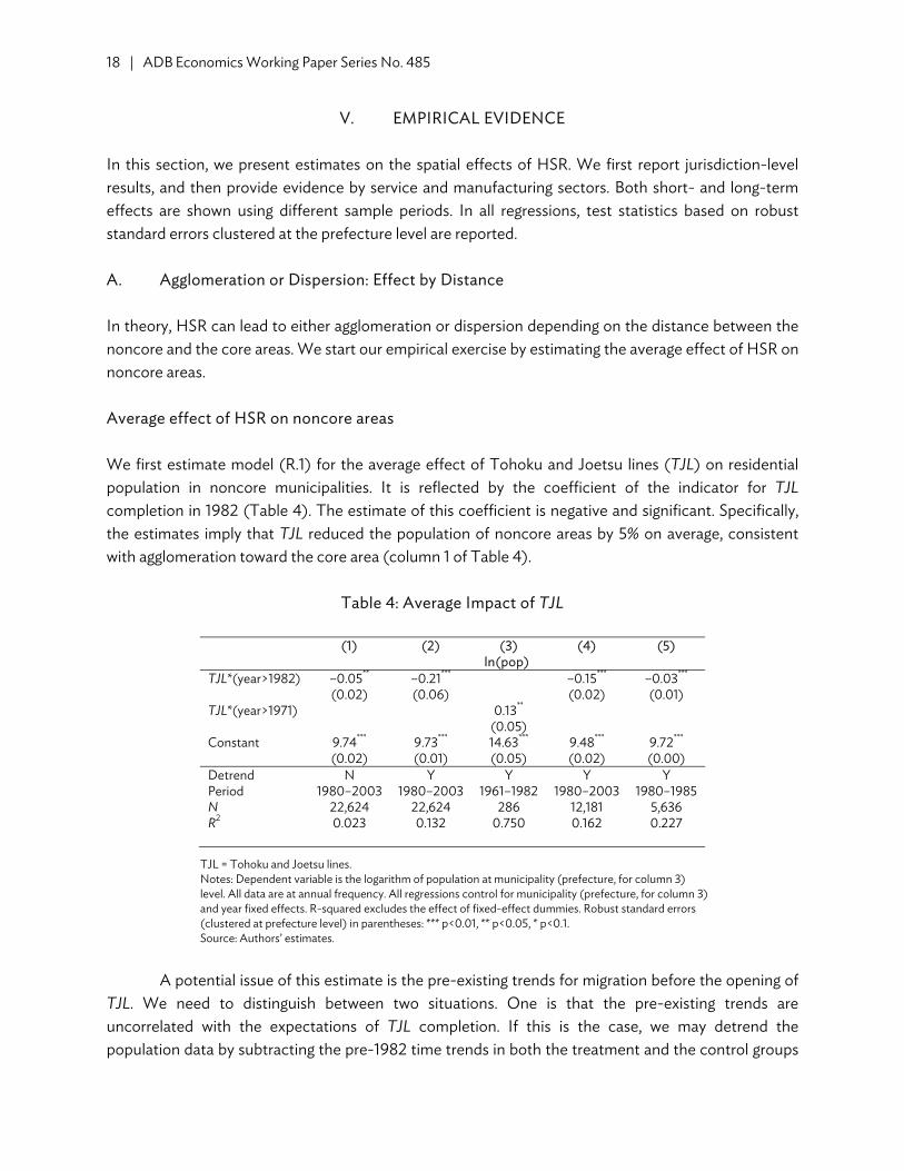
V. EMPIRICAL EVIDENCE In this section, we present estimates on the spatial effects of HSR. We first report jurisdiction-level results, and then provide evidence by service and manufacturing sectors. Both short- and long-term effects are shown using different sample periods. In all regressions, test statistics based on robust standard errors clustered at the prefecture level are reported. A. Agglomeration or Dispersion: Effect by Distance In theory, HSR can lead to either agglomeration or dispersion depending on the distance between the noncore and the core areas. We start our empirical exercise by estimating the average effect of HSR on noncore areas. Average effect of HSR on noncore areas We first estimate model (R.1) for the average effect of Tohoku and Joetsu lines (TJL) on residential population in noncore municipalities. It is reflected by the coefficient of the indicator for TJL completion in 1982 (Table 4). The estimate of this coefficient is negative and significant. Specifically, the estimates imply that TJL reduced the population of noncore areas by 5% on average, consistent with agglomeration toward the core area (column 1 of Table 4).

Table 4: Average Impact of TJL

(1) (2) (3) (4) (5) ln(pop)TJL*(year>1982) –0.05**

(0.02) –0.21***

(0.06) –0.15***

(0.02) –0.03*** (0.01)

TJL*(year>1971) 0.13**

(0.05)

Constant 9.74***

(0.02) 9.73***

(0.01) 14.63***

(0.05) 9.48***

(0.02) 9.72*** (0.00)

Detrend N Y Y Y Y Period 1980–2003 1980–2003 1961–1982 1980–2003 1980–1985 N 22,624 22,624 286 12,181 5,636 R2 0.023 0.132 0.750 0.162 0.227

TJL = Tohoku and Joetsu lines. Notes: Dependent variable is the logarithm of population at municipality (prefecture, for column 3) level. All data are at annual frequency. All regressions control for municipality (prefecture, for column 3) and year fixed effects. R-squared excludes the effect of fixed-effect dummies. Robust standard errors (clustered at prefecture level) in parentheses: *** p<0.01, ** p<0.05, * p<0.1. Source: Authors’ estimates.

A potential issue of this estimate is the pre-existing trends for migration before the opening of

TJL. We need to distinguish between two situations. One is that the pre-existing trends are uncorrelated with the expectations of TJL completion. If this is the case, we may detrend the population data by subtracting the pre-1982 time trends in both the treatment and the control groups


(column 2).22 With this approach, the estimated effect of TJL on the population increases to 0.21. This estimate implies that approximately three million residents in treated regions have migrated to Tokyo MA due to TJL, increasing the population of Tokyo MA by 10.5% and accounting for 44% of Tokyo MA population increase from 1982 to 2003.23

As another situation, the pre-existing migration trend of people might have been driven by the expectation of TJL. With the ministerial approval of TJL construction in 1971, people in noncore areas along TJL might expect population outflow and falling property prices. As a result, they could migrate to the core city even before the line was completed. To address this concern, we reestimate model (R.1) using prefecture population data, which cover 1961–1982 (data are detrended using data of 1950–1960). Instead of using 1982 as the start year of TJL, we use 1971, the year of approval. This estimate is to test whether the population agglomeration to Tokyo MA has already started after the approval of TJL project. The estimated coefficient of HSR is positive (column 3), contrasting our previous estimation. This is inconsistent with the hypothesized “approval effect” as discussed.

In column 4, we estimate the standard OLS model for comparison, without using the control

group. In this approach, the residential population is estimated to decline by 16% due to the TJL operation, which is slightly less than the DID estimate. Therefore, omitting the control group would bias our estimate of the TJL effect downward.

Previous estimates are for long-term effect over 2 decades following the completion of TJL. A

typical concern is that some other confounding factors arising during this long time period may bias our estimates, such as the housing price collapse. To address this concern, we conduct a series of estimates for different sample time periods. We find that the effect of TJL remained negative and gradually strengthened as time period lengthens (Figure 10). To illustrate, column 5 reports the estimate for 1980–1985, covering 3 years after the completion of TJL. The average impact on the population was estimated to be one-seventh of the estimate during 1980–2003, but remains statistically significant. Effects by Distance An important implication of theory is that the effect of HSR on a noncore area varies by its distance to the core area. When distance is long, HSR leads to agglomeration toward the core city; when distance is short, rising urban costs due to congestion effect dominate the agglomeration force, leading to decentralization.

22 As the municipality-level data series have only 2 years of observations before 1982, we construct the pre-1982 trend by

using prefecture-level data. We first use the prefecture-level data from 1970 to 1980 to construct a (linear) projection of the population growth rate during 1980–2003 for each prefecture. We then detrend the original municipality population data by subtracting them by the prefecture-level population increase implied by pre-1982 trend.

23 During 1982–2003, population size of Tokyo MA increased from 28.7 to 35.5 million.


To have a first-pass check of the hypothesis, we plot the municipality-level population growth rates during 1982–2003 against the distances between municipalities and Tokyo (Figure 9). The population growth of municipalities in the treated group shows a negative relation with the distance to Tokyo, while there is a flat (or slightly positive) relationship for the control group. Next we examine the relationship more rigorously by estimating model (R.2) using detrended municipality-level data for 1980–2003. The coefficient of the three-way interaction between TJL, the D1982 indicators, and the distance to Tokyo is –0.19, meaning that the negative effect of TJL on the population of a noncore city becomes larger if it is further away from Tokyo (column 1 of Table 5). Together with the coefficient of the interaction of the TJL and post-1982 indicators, 0.86, the model suggests that municipalities near Tokyo (within 92 km (=e(0.86/0.19)) of central Tokyo) experienced a population increase as a consequence of TJL. By contrast, the population of more distant municipalities shrank. This finding is consistent with the model implication: the peripheral of the core area may benefit from its spillover because of the rising urban costs in the core city. As a robustness check, we conduct a regression using original municipality data without detrending (column 2). The estimates are smaller in magnitude, but show similar patterns to that of the previous regression. The implied “boundary” of the peripheral that benefit from the spillover effect in Tokyo MA is approximately 130 km from central Tokyo.

Figure 9: Population Growth in Treatment and Control Municipalities (TJL versus TL)

km = kilometer, TJL = Tohoku and Joetsu lines, TL = Tokaido line. Source: Authors’ calculations.

As shown in Figure 9, municipalities in the treatment group tend to be more remote to Tokyo.

We estimate (R.2) using municipalities with a common support, namely, with similar distances to Tokyo. Results presented in column 3 are essentially unchanged. Moreover, as some municipalities in the control group (mostly in regions around Nagoya and Osaka) experienced rapid population growth in the study period, they might have a significant influence on our results. Column 4 gives the estimates by excluding these outliers (population growth during 1982–2003 exceeds 50% or –50%), and we find

TJL population growth

Distance_Tokyo (km)

ln(p

op. 2

003)

-ln(p

op. 1

982)

ln(p

op. 2

003)

-ln(p

op. 1

982)

–1

–.5

0

.5

1

–1

–.5

0

.5

1

100 200 300 400 5000 200 400 600 800

Distance_Tokyo (km)

TL population growth


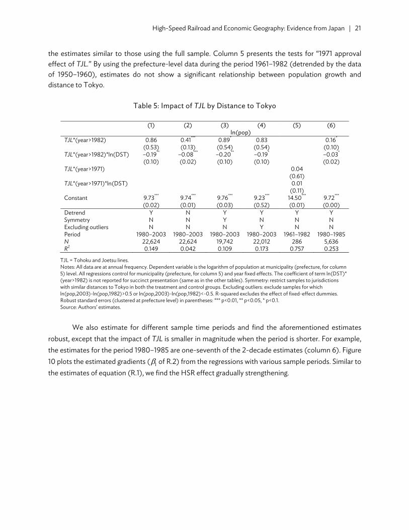
the estimates similar to those using the full sample. Column 5 presents the tests for “1971 approval effect of TJL.” By using the prefecture-level data during the period 1961–1982 (detrended by the data of 1950–1960), estimates do not show a significant relationship between population growth and distance to Tokyo.

Table 5: Impact of TJL by Distance to Tokyo

(1) (2) (3) (4) (5) (6) ln(pop)TJL*(year>1982) 0.86

(0.53) 0.41***

(0.13) 0.89*

(0.54) 0.83

(0.54) 0.16*

(0.10) TJL*(year>1982)*ln(DST) –0.19**

(0.10) –0.08***

(0.02) –0.20**

(0.10) –0.19*

(0.10) –0.03*

(0.02) TJL*(year>1971) 0.04

(0.61) TJL*(year>1971)*ln(DST) 0.01

(0.11) Constant 9.73***

(0.02) 9.74***

(0.01) 9.76***

(0.03) 9.23***

(0.52) 14.50*** (0.01)

9.72***

(0.00) Detrend Y N Y Y Y YSymmetry N N Y N N NExcluding outliers N N N Y N NPeriod 1980–2003 1980–2003 1980–2003 1980–2003 1961–1982 1980–1985N 22,624 22,624 19,742 22,012 286 5,636R2 0.149 0.042 0.109 0.173 0.757 0.253

TJL = Tohoku and Joetsu lines. Notes: All data are at annual frequency. Dependent variable is the logarithm of population at municipality (prefecture, for column 5) level. All regressions control for municipality (prefecture, for column 5) and year fixed effects. The coefficient of term ln(DST)* (year>1982) is not reported for succinct presentation (same as in the other tables). Symmetry: restrict samples to jurisdictions with similar distances to Tokyo in both the treatment and control groups. Excluding outliers: exclude samples for which ln(pop,2003)-ln(pop,1982)>0.5 or ln(pop,2003)-ln(pop,1982)<-0.5. R-squared excludes the effect of fixed-effect dummies. Robust standard errors (clustered at prefecture level) in parentheses: *** p<0.01, ** p<0.05, * p<0.1. Source: Authors’ estimates.

We also estimate for different sample time periods and find the aforementioned estimates

robust, except that the impact of TJL is smaller in magnitude when the period is shorter. For example, the estimates for the period 1980–1985 are one-seventh of the 2-decade estimates (column 6). Figure 10 plots the estimated gradients ( 1 of R.2) from the regressions with various sample periods. Similar to the estimates of equation (R.1), we find the HSR effect gradually strengthening.


Figure 10: The Estimated Coefficients of Equations (R.1) and (R.2) with Different Sample Periods

Note: The coefficients are based on the estimations with detrended data. Source: Authors’ calculations.

In the foregoing exercises, we assume that the effects of HSR on different people are the same.

Nevertheless, the working-age population should be much more responsive to HSR than the youth and the aged. To test this implications, we group the population as the youth (<15 years old), the aged (>64 years old), and the working age (15–64 years old), and run the baseline regressions on each group separately (Table 6). Consistent with the expectation, we find that the estimate for the working-age population is the most significant in terms of magnitude, doubling that for the full sample (column 1 of Table 6). The estimated gradient of agglomeration is also steeper for the working-age group (column 2 of Table 6). For the aged group, we find the HSR effects highly insignificant (columns 5–6 of Table 6). Interestingly, for the youth, we find smaller but qualitatively similar effects as the working-age population (columns 3–4 of Table 6). This could be because children follow their parents when they migrate, while the elderly stay behind. These findings by different age groups suggest that the patterns we find are likely to be job related, but not due to the change of general living amenities.

Table 6: Heterogeneity of the HSR Effects in Terms of Age

(1) (2) (3) (4) (5) (6) ln(pop): Age 15–64 ln(pop): Age <15 ln(pop): Age >64 TJL*(year>1982) –0.10**

(0.05) 2.19***

(0.57) –0.03(0.02)

1.28*

(0.78) –0.01

(0.03) –0.07 (0.42)

TJL*(year>1982)*ln(DST)

–0.41***

(0.10) –0.24*

(0.14) 0.01

(0.08) Constant 9.20***

(0.02) 9.22***

(0.02) 8.10***

(0.01) 8.14***

(0.00) 7.47*** (0.02)

7.47*** (0.02)

N 14,575 14,575 14,477 14,477 14,575 14,575 R2 0.091 0.107 0.728 0.729 0.929 0.929

HSR = High-Speed Railroad, TJL = Tohoku and Joetsu lines. Notes: Data are not detrended. Time coverage: 1980–2003 at annual frequency. All regressions control for municipality and year fixed effects. R-squared excludes the effect of fixed-effect dummies. Robust standard errors (clustered at prefecture level) in parentheses: *p< 0.1, **p< 0.05, ***p< 0.01. Source: Authors’ estimates.

–0.25

–0.20

–0.15

–0.10

–0.05

0.00

1980–1985 1980–1991 1980–1997 1980–2003

α1 of (R.1) β1 of (R.2)


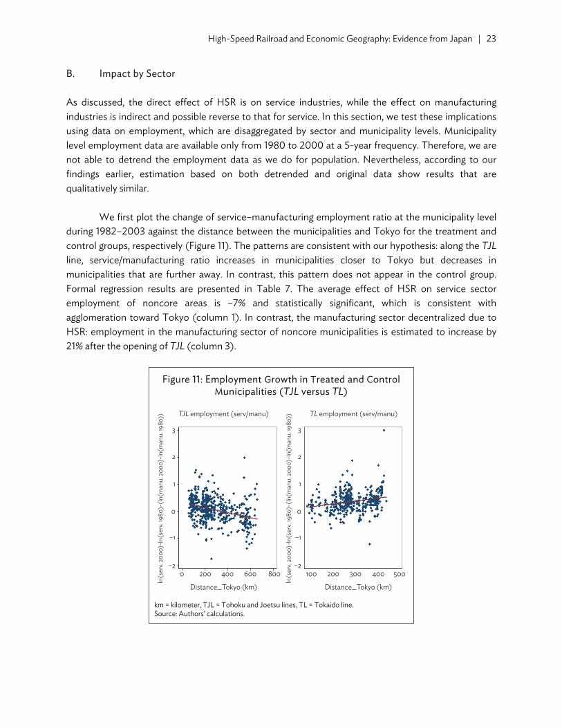
B. Impact by Sector As discussed, the direct effect of HSR is on service industries, while the effect on manufacturing industries is indirect and possible reverse to that for service. In this section, we test these implications using data on employment, which are disaggregated by sector and municipality levels. Municipality level employment data are available only from 1980 to 2000 at a 5-year frequency. Therefore, we are not able to detrend the employment data as we do for population. Nevertheless, according to our findings earlier, estimation based on both detrended and original data show results that are qualitatively similar.

We first plot the change of service–manufacturing employment ratio at the municipality level during 1982–2003 against the distance between the municipalities and Tokyo for the treatment and control groups, respectively (Figure 11). The patterns are consistent with our hypothesis: along the TJL line, service/manufacturing ratio increases in municipalities closer to Tokyo but decreases in municipalities that are further away. In contrast, this pattern does not appear in the control group. Formal regression results are presented in Table 7. The average effect of HSR on service sector employment of noncore areas is –7% and statistically significant, which is consistent with agglomeration toward Tokyo (column 1). In contrast, the manufacturing sector decentralized due to HSR: employment in the manufacturing sector of noncore municipalities is estimated to increase by 21% after the opening of TJL (column 3).

Figure 11: Employment Growth in Treated and Control Municipalities (TJL versus TL)

km = kilometer, TJL = Tohoku and Joetsu lines, TL = Tokaido line. Source: Authors’ calculations.

TJL employment (serv/manu) TL employment (serv/manu)

Distance_Tokyo (km)

ln(s

erv.

2000

)-ln

(ser

v. 19

80)-

(ln(m

anu.

200

0)-ln

(man

u. 19

80))

ln(s

erv.

2000

)-ln

(ser

v. 19

80)-

(ln(m

anu.

200

0)-ln

(man

u. 19

80))

0 100 200 300 400 500200–2

–1

0

1

2

3

–2

–1

0

1

2

3

400 600 800

Distance_Tokyo (km)


Table 7: Impact of TJL by Service and Manufacturing Industries

(1) (2) (3) (4) ln(service employ) ln(manu. employ) TJL*(year>1982) –0.07**

(0.03) 0.72***

(0.18) 0.19***

(0.05) –0.99** (0.38)

TJL*(year>1982)*ln(DST)

–0.14***

(0.03) 0.21*** (0.07)

Constant 7.92***

(0.01) 7.92***

(0.01) 7.35***

(0.02) 7.35*** (0.02)

N 4,714 4,714 4,714 4,714 R2 0.472 0.487 0.188 0.198

TJL = Tohoku and Joetsu lines. Notes: Data is not detrended. Time period is 1980–2000 at 5-year frequency. All regressions control for municipality and year fixed effects. “service employ” contains the aggregated employment of finance, insurance, real estate, transportation and telecom, public service, wholesale and retail, and the other unclassified services. R-squared excludes the effect of fixed-effect dummies. Robust standard errors (clustered at prefecture level) in parentheses: *** p<0.01, ** p<0.05, * p<0.1. Source: Authors’ estimates.

We then estimate the effect of TJL on municipalities with different distances to Tokyo (columns 2 and 4). The estimates for the service sector confirm the downward “gradients” in the TJL effect. Service employment increased in regions within 171 km (=e0.72/0.14) of Tokyo according to the estimate, but shrunk in those beyond. In contrast, the manufacturing sector demonstrates economic downsizing in the areas within 111 km (=e0.99/0.21) of Tokyo and economic upsizing for areas beyond.24 C. Robustness Checks Alternative Control Groups Following a common empirical strategy in the literature, we also further examine the impact of HSR on municipalities with different distances to a TJL station (column 1 of Table 8). Dummy variables indicating whether a municipality is within 60 km from an HSR station or greater than 60 km from an HSR station are interacted with the indicator of HSR completion and TJL dummy. We find that municipalities within 60 km suffer the most from the impact of HSR, while municipalities that are 60 km or further away from TJL show insignificant impact.

The control group of our baseline regressions includes prefectures along the Tokaido line. As a robustness check, we consider an alternative control group, which includes jurisdictions along the Hokuriku line (Ishikawa, Nagano, and Toyama prefectures). Hokuriku line, connecting three prefectures in the western region to Tokyo, was partly operated since 1997 with a length of 117 km

24 For the estimates using employment data to be comparable with those using population data, we repeat the regression for

population, using observations in the same years as those for the employment data. We find that the estimate for this subsample of population is almost the same as that for the full sample (results are available upon request).


(blue line in Figure 12[b]); the completed route is 345 km and has been in full operation since 2015.25 Both the regions covered by the Hokuriku line (circled HL in Figure 12 [a]) and the Joetsu line (circled JL in Figure 12 [a]) are in inland Japan and are mountainous.26 Moreover, the Hokuriku line does not involve large cities, which could affect the estimates. The disadvantage is that Hokuriku line did not open until 1997. Hence, between 1982 and 1997, economic shocks to the Tokyo economy may have different spillover effects on jurisdictions along the Joetsu line and the Hokuriku line. In this case, the DID approach is not able to eliminate these confounding spillover effects.

Figure 12: Impact of Joetsu Line: Taking the Planned Hokuriku Line as the Control

(a) (b)

Notes: Joetsu line (red line in Figure [b]); Hokuriku line (blue line in Figure [b]); In our robustness tests, we consider only the part of Joetsu line between Niigata and Takasaki as the treated area, because the Joetsu line overlaps with the Hokuriku line between Takasaki and Tokyo. Source: Constructed by the authors.

Figure 13 presents the population growth dynamics by distance to Tokyo during 1982–1996

(before the opening of the Hokuriku line in 1997), we find similar trends as those in the original treated and control groups. The estimates using data from 1980 to 1996 are reported in Table 8. These estimates are all consistent with our baseline results. After the opening of the Joetsu line in 1982, municipalities along this line experienced a significant population loss compared with that in regions along the planned Hokuriku line (column 2). We also examine the effects of HSR by service and manufacturing sectors in columns 3–4. Service employment agglomerates to areas close to Tokyo, which is in line with our baseline results. For manufacturing, we find the estimates under this specification become insignificant.

25 Hokuriku line shares the same route with Joetsu line for the part of Takasaki–Tokyo, as shown in Figure 12. 26 Note that we keep only the prefectures along Joetsu line as the treatment group in this exercise for comparability.


Figure 13: Population Growth in Treatment and Control Municipalities (JL versus HL)

HL = Hokuriku line, JL = Joetsu line, km = kilometer. Source: Authors’ calculations.

Table 8: Estimates with Alternative Control Groups

(1) (2) (3) (4) ln(pop) ln(pop) ln(service employ) ln(manu. employ)

JL*(year>1982) 0.33***

(0.09) 0.63***

(0.09) 0.53

(0.52) JL*(year>1982)*ln(DST) –0.07***

(0.02) –0.12***

(0.02) –0.08(0.10)

TJL*(year>1982)*HSR station(<60km) –0.06***

(0.02)

TJL*(year>1982)*HSR station(≥60km) –0.03(0.04)

(year>1982)*HSR station(<60km) 0.02(0.02)

(year>1982)*HSR station(≥60km) –0.01(0.04)

Constant 9.74***

(0.01) 9.28***

(0.00) 7.42***

(0.00) 6.89***

(0.01) Samples: Treated & Control TJL&TL JL&HL JL&HL JL&HLPeriod 1980–2003 1980–1996 1980–1995 1980–1995Data frequency annual annual 5-year 5-yearN 22,624 6,290 1,480 1,480 R2 0.025 0.048 0.466 0.150

HL = Hokuriku line, HSR = High-Speed Railroad, JL = Joetsu line, km = kilometer, TJL = Tohoku and Joetsu lines. Notes: All regressions control for municipality and year fixed effects. JL: Niigata and Gumma prefectures, which are along the Joetsu line; HL: Toyama, Nagano and Ishikawa prefectures, which are along the Hokuriku line. R-squared excludes the effect of fixed-effect dummies. Robust standard errors (clustered at prefecture level) in parentheses: *** p<0.01, ** p<0.05, * p<0.1. Source: Authors’ estimates.

JL population growth HL population growth

Distance_Tokyo (km)

ln(p

op. 1

996)

-ln(p

op. 1

982)

ln(p

op. 1

996)

-ln(p

op. 1

982)

50–.6

–.3

0

.3

.6

–.6

–.3

0

.3

.6

100 150 200 250 300100 150 200 250 300

Distance_Tokyo (km)


Controlling for Highway Investment During our sample period, the highway length of treated prefectures grew from 7,266 to 10,052 km, and that of control prefectures increased from 4,510 to 6,165 km. To address the concern that these highway investments could bias our estimates due to simultaneity, we augment the baseline regressions by further controlling for highway investments. Specifically, we use the data from Japan Statistical Yearbook 1982–2006 on national highway length at prefecture level (1980–2003) as a proxy of highway stock. As shown in Table 9, the estimates of highway control are positive and significant, contrasting sharply with the HSR effect. Moreover, the key coefficients are essentially unchanged compared with the baseline estimates.

Due to data constraint, we are not able to examine the confounding effect of conventional railroad. Nevertheless, as discussed earlier, they have changed little during our sample period at the national level, so their confounding effect should be limited.

Table 9: Control for the Effect of the National Highway

(1) (2) (3) ln(pop) ln(service employ) ln(manu. employ) TJL*(year>1982) –0.05**

(0.02) –0.07**

(0.04) 0.20***

(0.05) ln(HWY) 0.24*

(0.14) 0.35*

(0.21) –0.39(0.41)

Constant 8.11***

(0.95) 5.25***

(1.41) 10.02***

(2.76) Period 1980–2003 1980–2000 1980–2000 Data frequency annual 5-year 5-yearN 22,624 4,714 4,714R2 0.028 0.474 0.189

TJL = Tohoku and Joetsu lines. Notes: ln(HWY): logarithm of the stock of national highway length (km) at prefecture level. Data are not detrended. Time period: 1980–2003 at annual frequency for population and 1980–2000 at 5-year frequency for employment. All regressions control for municipality and year fixed effects. R-squared excludes the effect of fixed-effect dummies. Robust standard errors (clustered at prefecture level) in parentheses: *** p<0.01, ** p<0.05, * p<0.1. Source: Authors’ estimates.

Osaka Effect As our major control group includes Osaka, the second largest city in Japan, our estimates could be affected for two reasons. First, given the size of Osaka, it could have significant economic linkage with its nearby areas. This is inconsistent with the setup of our model, in which we assume noncore areas trade with Tokyo MA only. Second, the Sanyo line was completed in 1972 to extend the Tokaido line from Osaka toward the further south of Japan (Fukuoka). Osaka being the largest city on this line could also experience the agglomeration from jurisdictions along the Sanyo line.


To address the potential confounding effects of Osaka, we first check the robustness of our estimates by excluding Osaka (Table 10). The estimates are generally consistent with our baseline results. Alternatively, we provide direct evidence on the effect of the Sanyo line on Osaka. The regression is similar to those in previous exercises (regression models R.1 and R.2), except that our treatment group is now prefectures along the Sanyo line, while the control group is prefectures along the Tokaido line (excluding Tokyo MA and Osaka). Our sample period is from 1960 to 2000 (prefecture level).

We find that the Sanyo line led to a population decline of 8% in non-Osaka areas (column 1 of Table 11); however, we do not find significant effect of the distance to Osaka (column 2). We also test with shorter (1960–1980, 1960–1990) time periods and find similar results.27 These findings suggest that the Sanyo line did induce a population loss in areas to the south of Osaka, although it is unclear whether the lost population moved to Osaka. This could be because Osaka was not a core area, while Tokyo was. This is in line with the descriptive evidence presented by Mori (2012): after the opening of the Tokaido and Sanyo lines, Osaka MA shrunk because of greater agglomeration to Tokyo MA.

Table 10: Baseline Results: Excluding Osaka

(1) (2) (3) ln(pop) ln(service employ) ln(manu. employ) TJL*(year>1982) 0.36**

(0.15) 0.71***

(0.23) –0.78* (0.47)

TJL*(year>1982)*ln(DST) –0.07***

(0.03) –0.14***

(0.04) 0.17*

(0.09) Constant 9.62***

(0.01) 7.78***

(0.01) 7.21*** (0.02)

Period 1980–2003 1980–2000 1980–2000 Data frequency annual 5-year 5-year N 21,042 4,385 4,385 R2 0.045 0.487 0.196

TJL = Tohoku and Joetsu lines. Notes: Data are not detrended. All regressions control for municipality and year fixed effects. R-squared excludes the effect of fixed-effect dummies. Robust standard errors (clustered at prefecture level) in parentheses: *** p<0.01, ** p<0.05, * p<0.1. Source: Authors’ estimates.

27 As we use prefecture-level data here, which is different from our main estimations (municipality-level data), we also

repeat our baseline exercises using prefecture-level data to ensure the comparability of the estimates. We find that the regression results with prefectures are highly consistent with our results based on the municipality-level data (see columns 3 and 4 of Table 11).


Table 11: Robustness Check: Prefecture-Level Data

(1) (2) (3) (4) ln(pop_pref)SL*(year>1975) –0.08**

(0.04) –0.04(0.22)

SL*(year>1975)*ln(DST_Osaka)

–0.01(0.04)

TJL*(year>1982)

–0.09**

(0.04) 0.45*

(0.25) TJL*(year>1982)*ln(DST)

–0.10** (0.05)

Constant 14.77***

(0.01) 14.74***

(0.01) 14.69***

(0.01) 14.66*** (0.24)

Samples: Treated & Control SL&TL SL&TL TJL&TL TJL&TL N 410 410 533 533 R2 0.841 0.851 0.741 0.777

SL = Sanyo line, TJL = Tohoku and Joetsu lines, TL = Tokaido line. Notes: Dependent variable is the logarithm of population at prefecture level. Time period: 1960–2000 at annual frequency. All regressions control for prefecture and year fixed effects. TJL: Tohoku and Joetsu lines; TL: Tokaido line; SL: Sanyo line. Sanyo line (SL) between Osaka and Fukuoka opened up in 1975; Columns 1–2 contain samples of TL (Shizuoka, Shiga, Gifu, Aichi, Kyoto) and SL (Hyogo, Okayama, Yamaguchi, Hiroshima, Fukuoka), by excluding Osaka, since both TL and SL are connected to Osaka; Columns 3–4 contain samples of TJL (Aomori, Iwate, Miyagi, Fukushima, Tochigi, Niigata, Gumma) and TL (Shizuoka, Shiga, Gifu, Aichi, Kyoto, Osaka), by excluding Tokyo MA, since both TJL and TL are connected to Tokyo MA. Distance measure is based on the distance between Tokyo/Osaka downtown and core city of each prefecture. Robust standard errors (clustered at prefecture level) in parentheses: *** p<0.01, ** p<0.05, * p<0.1. Source: Authors’ estimates.

VI. CONCLUSION

This study shows that the spatial impact of HSR is not a simple polarization or diffusion relationship, but depends on the nature of industries and the distance between cities. We first illustrate this utilizing a core-periphery model, in which passengers can travel across regions to purchase service goods. As HSR reduces the interregional travel costs for passengers, the service sector with increasing returns to scale may agglomerate toward the core city if its distance with the noncore city is large; if the distance is sufficiently small, HSR leads to decentralization of the service sector. The impact of HSR on the manufacturing sector may be the reverse, even though it is not directly affected by HSR. Specifically, when urban costs are present, HSR may push the manufacturing sector out of the core region toward distant noncore areas.

These hypotheses are supported by our empirical evidence based on the municipality (or prefecture) residential and employment data from Japan. Utilizing the completion of HSR in Japan in 1982 as a quasi-experiment, we conduct DID estimation with jurisdictions along new HSR as a treatment group, and those along the existing HSR as a control group. We find significant agglomeration of service industries toward Tokyo MA and its peripheral cities following the completion of HSR. Due to the impact of the new HSR, the total scale of Tokyo MA increased by as much as


10.5%. The outskirt of Tokyo MA benefited even more than the Tokyo core. In contrast, manufacturing industries decentralize toward distant noncore areas. These effects are consistent with theory implications. They persist in both short and long terms.

These findings reconcile contrasting findings in the literature: while some researchers find that

HSR leads to agglomeration, some other show evidence on decentralization, depending on the sector and spatial scope examined by researchers. Moreover, this study also has implications regarding growth strategies. One concerns the inclusive growth. A common hypothesis by governments investing in high-speed railroad is to help improve the growth of distant regions (e.g., DFT 2011, for the UK). Although HSR may improve people’s mobility and choices of service products, we find no evidence that employment increases in distant areas. In fact, more distant noncore cities are likely to lose jobs in the service sector, and this is only partly offset by the decentralization of manufacturing sector. Moreover, the urbanization strategy of developing countries may also be affected by HSR: the surging HSR investments may generate significant economic agglomeration and formation of mega cities due to further agglomeration in service industries. This can have profound implications for urban policies on society, demographics, and environment in the face of the rising wave of high-speed railroad investment around the globe, especially in developing countries.

REFERENCES Ahlfeldt, G., and A. Feddersen. 2010. From Peripheral to Core: Economic Adjustment to High Speed

Rail. London School of Economics. Mimeo. Alonso, W. 1964. Location and Land Use. Cambridge: Harvard University Press. Baum-Snow, N. 2007. Did Highways Cause Suburbanization? Quarterly Journal of Economics. 122 (2).

pp. 775–805. ————. 2014. Urban Transport Expansions, Employment Decentralization, and the Spatial Scope of

Agglomeration Economies. Brown University. Mimeo. Baum-Snow, N., L. Brandt, J. V. Henderson, M. A. Turner, and Q. Zhang. 2014. Roads, Railways and

Decentralization of Chinese Cities. Brown University. Mimeo. Bernard, A. B., A. Moxnes, Y. U. Saito. 2015. Production Networks, Geography and Firm Performance.

NBER Working Paper No. 21082. Center for Spatial Information Science, The University of Tokyo (Geocoding Tools & Utilities).

http://newspat.csis.u-tokyo.ac.jp/geocode (accessed 11 November 2014).

Chen, C.-L., and P. Hall. 2011. The Impacts of High-Speed Trains on British Economic Geography: A Study of the UK’s InterCity 125/225 and Its Effects. Journal of Transport Geography. 19 (4). pp. 689–704.

————. 2012. The Wider Spatial-Economic Impacts of High-Speed Trains: A Comparative Case Study

of Manchester and Lille Sub-Regions. Journal of Transport Geography. 24. pp. 89–110. Department for Transport (DFT). 2011. High Speed Rail: Investing in Britain’s Future Consultation.

London, United Kingdom. Faber, B. 2014. Trade Integration, Market Size, and Industrialization: Evidence from China’s National

Trunk Highway System. Review of Economic Studies. 81 (3). pp. 1046–70. Fujita, M. 1989. Urban Economic Theory: Land Use and City Size. Cambridge: Cambridge University

Press. Fujita, M., P. Krugman, and A. J. Venables. 1999. The Spatial Economy: Cities, Regions, and

International Trade. Cambridge: The MIT Press. ADB recognizes “China” as the People’s Republic of China.

32 | References

Fujita, M., T. Mori, J. V. Henderson, and Y. Kanemoto. 2004. Spatial Distribution of Economic

Activities in Japan and China. In J. V. Henderson, and J. F. Thisse, eds. Handbook of Regional and Urban Economics, edition 1, volume 4, chapter 65, pp. 2911–2977.

House of Commons. 2011. High Speed Rail: Tenth Report of Session 2010–12. London. Japan Railway Company. 2001. Shinkansen Time Table in 2001. Japan. ————. 2010. Japan High Speed Rail Passenger Traffic Statistics. Japan.

Japan Times. 1965. New Tokaidowill Reach Hakata in '75. March 20, 1965: 4. ————. 1967. JNR Reveals 20-Yr. Plan for more “Bullet Trains”. 1 September: 4. ————. 1971. Move on New Tohoku Line Seen Soon. 2 October: 3. Krugman, P. 1991. Increasing Returns and Economic Geography. Journal of Political Economy. 99 (31):

483–99. Leclerc, R. 2002. A Geographical Study of the Emergence of the High-Speed Train and His Effects on

Land Management and Regional Economic Development in Japan: http://www.ebc.qc.ca/ documents/shinkansen.pdf

Miyawaki, S. 1998. The History of Railways Followed by Time Table (in Japanese) (Jikokuhyou de

tadoruTetsudoushi). Tokyo: JTB Press. Mori, T. 2012. Increasing Returns in Transportation and the Formation of Hubs. Journal of Economic

Geography. 12 (4). pp. 877–97. Murakami, J., and R. Cervero. 2012. High-speed Rail and Economic Development: Business

Agglomeration and Policy Implications. UC Berkeley. Mimeo. Murata, Y., and J.-F. Thisse. 2005. A Simple Model of Economic Geography à la Helpman-Tabuchi.

Journal of Urban Economics. 58 (1). pp. 137–55. Okada, H. 1994. Features and Economic and Social Effects of the Shinkansen. Japan Railway and

Transport Review. 10. pp. 9–16. Ottaviano, G. I. P., T. Tabuchi, and J.-F. Thisse. 2002. Agglomeration and Trade Revisited. International

Economic Review. 43 (2). pp. 409–435.

References | 33

Qin, Y. 2014. “No County Left Behind?” The Distributional Impact of High-Speed Rail Upgrade in

China. National University of Singapore. Mimeo. Rothenberg, A. 2011. Transport Infrastructure and Firm Location Choice in Equilibrium: Evidence from

Indonesia’s Highways. UC Berkeley. Mimeo. Sasaki, K., T. Ohashi, and A. Ando. 1997. High-Speed Rail Transit Impact on Regional Systems: Does

the Shinkansen Contribute to Dispersion? Annals of Regional Science. 31 (1). pp. 77–98. Shozawa, H. 2011. Essential Knowledge of Japanese National Railways: 1945–1987 (in Japanese)

(Kokutetsu no Kisochishiki). Osaka: Sogensha. Smith, R. A. 2003. The Japanese Shinkansen: Catalyst for the Renaissance of Rail. Journal of Transport

History. 24 (2). pp. 222–37. Statistics Bureau, Ministry of Internal Affairs and Communication. Various years. Japan Statistical

Yearbook. Japan. ————. Various years. Japan Urban Statistical Yearbook. Japan. ————. Various years. Population Census of Japan. Japan. Tabuchi, T. 1998. Urban Agglomeration and Dispersion: A Synthesis of Alonso and Krugman. Journal of

Urban Economics. 44 (3). pp. 333–51. Tabuchi, T., and J.-F. Thisse. 2006. Regional Specialization, Urban Hierarchy, and Commuting Costs.

International Economic Review. 47 (4). pp. 1295–1317. Tang, J. P. 2014. Railroad Expansion and Industrialization: Evidence from Meiji Japan. Journal of

Economic History. 74 (3). pp. 863–86. US High Speed Rail Association. 2014. High Speed Lines in the World. http://www.uic.org/IMG/pdf/

20140901_high_speed_lines_in_the_world.pdf

ASIAN DEVELOPMENT BANK

AsiAn Development BAnk6 ADB Avenue, Mandaluyong City1550 Metro Manila, Philippineswww.adb.org

High-Speed Railroad and Economic Geography: Evidence from Japan

We study whether high-speed railroad (HSR) polarizes or balances economic geography using the 1982 opening of two major HSRs in Japan (Shinkansen). We find that both agglomeration and decentralization could occur. While service industry tends to agglomerate toward the core city, manufacturing industry may decentralize toward peripheral cities. We estimate that in noncore areas of Japan, service employment decreased by 7%, while manufacturing employment increased by 21%. Moreover, proximity between peripheral and core cities also matter. Cities within approximately 100 kilometers of Tokyo expanded, while more distant cities shrank. The net result is that Tokyo metropolitan area agglomerates because of HSR.

About the Asian Development Bank

ADB’s vision is an Asia and Pacific region free of poverty. Its mission is to help its developing member countries reduce poverty and improve the quality of life of their people. Despite the region’s many successes, it remains home to the majority of the world’s poor. ADB is committed to reducing poverty through inclusive economic growth, environmentally sustainable growth, and regional integration.

Based in Manila, ADB is owned by 67 members, including 48 from the region. Its main instruments for helping its developing member countries are policy dialogue, loans, equity investments, guarantees, grants, and technical assistance.

adb economicsworking paper series

NO. 485

may 2016

HiGH-SpEED RAilROAD AND EcONOmic GEOGRApHy: EviDENcE fROm JApANZhigang Li and Hangtian Xu

high-speed railroad and economic geography: evidence … · adb economics working paper series...

Documents