HIGHER ORDER SYMPLECTIC METHODS FORSEPARABLE HAMILTONIAN EQUATIONS

A Thesis Submitted tothe Graduate School of Engineering and Sciences of

Izmir Institute of Technologyin Partial Fulfillment of the Requirements for the Degree of

MASTER OF SCIENCE

in Mathematics

byHakan GUNDUZ

July 2010IZMIR

We approve the thesis of Hakan GUNDUZ

Assoc. Prof. Dr. Gamze TANOGLUSupervisor

Assoc. Prof. Dr. Ali Ihsan NESLITURKCommittee Member

Assist. Prof. Dr. H. Secil ARTEMCommittee Member

5 July 2010

Prof. Dr. Oguz YILMAZ Assoc. Prof. Dr. Talat YALCINHead of the Department of Dean of the Graduate School ofMathematics Engineering and Sciences

ACKNOWLEDGMENTS

This thesis is the consequence of a three-year study evolved by the contribution

of many people and now I would like to express my gratitude to all the people supporting

me from all the aspects for the period of my thesis.

Firstly, I would like to thank and express my deepest gratitude to Assoc. Prof. Dr.

Gamze TANOGLU, my advisor, for her help, guidance, understanding, encouragement

and patience during my studies and preparation of this thesis.

Secondly, thanks to Nurcan GUCUYENEN and Duygu DEMIR for their supports.

I am also thankful to Barıs CICEK, for his help whenever I needed. And finally I am

grateful to my family for their confidence to me and for their endless supports.

ABSTRACT

HIGHER ORDER SYMPLECTIC METHODS FOR SEPARABLE HAMILTONIANEQUATIONS

The higher order, geometric structure preserving numerical integrators based on

the modified vector fields are used to construct discretizations of separable Hamiltonian

systems. This new approach is called as modifying integrators. Modified vector fields

can be used to construct high-order structure-preserving numerical integrators for both

ordinary and partial differential equations. In this thesis, the modifying vector field idea is

applied to Lobatto IIIA-IIIB methods for linear and nonlinear ODE problems. In addition,

modified symplectic Euler method is applied to separable Hamiltonian PDEs. Stability

and consistency analysis are also studied for these new higher order numerical methods.

Von Neumann stability analysis is studied for linear and nonlinear PDEs by using modi-

fied symplectic Euler method. The proposed new numerical schemes were applied to the

separable Hamiltonian systems.

iv

OZET

AYRILABILIR HAMILTON DENKLEMLER ICIN YUKSEK MERTEBEDENSIMPLEKTIK METODLAR

Yuksek mertebeden, modifiye edilmis vektor alanını esas alan geometrik yapıyı

koruyan numerik integratorler, ayrılabilir Hamilton sistemlerin diskritizasyonu icin kulla-

nılmıstır. Bu yeni yaklasım modifiye edilmis integrator olarak adlandırılır. Modifiye

vektor alanları tum adi ve kısmi diferansiyel denklemler icin yuksek mertebeden yapıyı

koruyan numerik integratorlerin olusturulmasında kullanılabilir. Bu tezde, linear ve lin-

ear olmayan adi diferansiyel denklemler icin Lobatto IIIA-IIIB metodlarına modifiye

edilmis vektor alanı uygulanmıstır. Ek olarak, modifiye edilmis simplektik Euler metodu

ayrılabilir Hamilton kısmi diferansiyel denklemlerine uygulandı. Ayrıca bu yeni yuksek

mertebeden numerik metodlar icin kararlılık ve tutarlılık analizleri uzerine calısıldı. Von

Neumann kararlılık analizi linear ve linear olmayan Hamilton kısmi diferansiyel den-

klemlerine modifiye edilmis simplektik Euler metodu kullanılarak calısıldı. Sunulan yeni

numerik semalar ayrılabilir hamilton sistemlerine uygulandı.

v

5.2. Von-Neumann Stability Analysis Applied to Hamiltonian PDEs

37

2.1.1. Modified Equations for Backward Error Analysis

TABLE OF CONTENTS

LIST OF FIGURES . . . . . . . . . . . . . . . . . . . . . . . . . . . . . . . . . . . . . . . . . . . . . . . . . . . . . . . . . . . . . . . . . . . . . . . viii

LIST OF TABLES . . . . . . . . . . . . . . . . . . . . . . . . . . . . . . . . . . . . . . . . . . . . . . . . . . . . . . . . . . . . . . . . . . . . . . . . x

CHAPTER 1. INTRODUCTION . . . . . . . . . . . . . . . . . . . . . . . . . . . . . . . . . . . . . . . . . . . . . . . . . . . . . . . 1

CHAPTER 2. BACKGROUND . . . . . . . . . . . . . . . . . . . . . . . . . . . . . . . . . . . . . . . . . . . . . . . . . . . . . . . . 3

2.1. Backward Error Analysis . . . . . . . . . . . . . . . . . . . . . . . . . . . . . . . . . . . . . . . . . . . . . 3

. . . . . . . . . . . . . . 3

2.2. Modifying Numerical Integrators . . . . . . . . . . . . . . . . . . . . . . . . . . . . . . . . . . . . 7

2.3. Symplectic Integrators . . . . . . . . . . . . . . . . . . . . . . . . . . . . . . . . . . . . . . . . . . . . . . . . 11

2.3.1. Examples of the Symplectic Methods . . . . . . . . . . . . . . . . . . . . . . . . . . . . 14

2.4. Geometric Properties . . . . . . . . . . . . . . . . . . . . . . . . . . . . . . . . . . . . . . . . . . . . . . . . . . 17

CHAPTER 3. CONSTRUCTION OF LOBATTO METHOD . . . . . . . . . . . . . . . . . . . . . . . . 19

3.1. Partitioned Runge-Kutta Methods . . . . . . . . . . . . . . . . . . . . . . . . . . . . . . . . . . . . 20

3.2. Lobatto IIIA - IIIB Pairs . . . . . . . . . . . . . . . . . . . . . . . . . . . . . . . . . . . . . . . . . . . . . . 22

3.3. Modified Lobatto Methods . . . . . . . . . . . . . . . . . . . . . . . . . . . . . . . . . . . . . . . . . . . . 23

CHAPTER 4. CONVERGENCE ANALYSIS . . . . . . . . . . . . . . . . . . . . . . . . . . . . . . . . . . . . . . . . . 31

4.1. Stability Analysis . . . . . . . . . . . . . . . . . . . . . . . . . . . . . . . . . . . . . . . . . . . . . . . . . . . . . .

4.1.1. The Behaviour of Stability of Modified Lobatto Method . . . . . . . 42

CHAPTER 5. MODIFIED SYMPLECTIC EULER METHOD FOR PDE

PROBLEMS . . . . . . . . . . . . . . . . . . . . . . . . . . . . . . . . . . . . . . . . . . . . . . . . . . . . . . . . . . . . . 44

5.1. Criteria of Linear Stability of Symplectic Algorithm . . . . . . . . . . . . . . . . 45

. . . . 46

5.2.1. Linear Wave Equation . . . . . . . . . . . . . . . . . . . . . . . . . . . . . . . . . . . . . . . . . . . . . 47

5.2.2. Sine-Gordon Equation . . . . . . . . . . . . . . . . . . . . . . . . . . . . . . . . . . . . . . . . . . . . 54

5.2.3. Schrodinger Equation . . . . . . . . . . . . . . . . . . . . . . . . . . . . . . . . . . . . . . . . . . . . . 56

vi

6.3. Numerical Results of Hamiltonian PDE Problems

in Hamiltonian and CPU Time

6.1.3.1. Comparison of the Norm of Global Error, Norm of Error

6.1. Numerical Results of Hamiltonian ODE Problems

CHAPTER 6. NUMERICAL EXPERIMENT . . . . . . . . . . . . . . . . . . . . . . . . . . . . . . . . . . . . . . . . . 60

. . . . . . . . . . . . . . . . . . 60

6.1.1. Applications to Harmonic Oscillator System . . . . . . . . . . . . . . . . . . . . 60

6.1.2. Modified Equations Based on Lobatto IIIA-IIIB Methods . . . . . . 60

6.1.3. Numerical Implementation for Harmonic Oscillation . . . . . . . . . . . 61

. . . . . . . . . . . . . . . . . . . . . . . . . . . . . 65

6.2. Applications to Double Well System . . . . . . . . . . . . . . . . . . . . . . . . . . . . . . . . . 66

6.2.1. Numerical Implementation for Double Well . . . . . . . . . . . . . . . . . . . . . 67

. . . . . . . . . . . . . . . . . . 70

6.3.1. Linear Wave Equation . . . . . . . . . . . . . . . . . . . . . . . . . . . . . . . . . . . . . . . . . . . . . 70

6.3.2. Sine-Gordon Equation . . . . . . . . . . . . . . . . . . . . . . . . . . . . . . . . . . . . . . . . . . . . 73

CHAPTER 7. CONCLUSION . . . . . . . . . . . . . . . . . . . . . . . . . . . . . . . . . . . . . . . . . . . . . . . . . . . . . . . . . . 80

REFERENCES . . . . . . . . . . . . . . . . . . . . . . . . . . . . . . . . . . . . . . . . . . . . . . . . . . . . . . . . . . . . . . . . . . . . . . . . . . . 82

APPENDIX A. MATLAB CODES FOR NUMERICAL EXPERIMENTS . . . . . . . . . . 84

vii

LIST OF FIGURES

Figure Page

Figure 2.1. Idea of Backward Error Analysis. . . . . . . . . . . . . . . . . . . . . . . . . . . . . . . . . . . . . . . . . . . 4

Figure 2.2. Exact, forward Euler and 1-term modified equation solutions to

y = y2, y(0) = 1. . . . . . . . . . . . . . . . . . . . . . . . . . . . . . . . . . . . . . . . . . . . . . . . . . . . . . . . . . . 5

Figure 2.3. Exact, forward Euler and m-term modified equation solutions to

y = y2, y(0) = 1 with step-size h = 2.10−2. . . . . . . . . . . . . . . . . . . . . . . . . . . . . . 6

Figure 2.4. Idea of Modified Differential Equations. . . . . . . . . . . . . . . . . . . . . . . . . . . . . . . . . . . 8

Figure 4.1. The relation between the parameter h and Tr(W ) for modified Lobatto

method applied to Harmonic oscillation problem. . . . . . . . . . . . . . . . . . . . . . . . . 43

Figure 5.1. The graph of y(α) = 2− α− α1−α

and y = 2. . . . . . . . . . . . . . . . . . . . . . . . . . . . . 52

Figure 6.1. Error in Hamiltonian and global error in Hamiltonian by Lobatto

IIIA-IIIB method of order 2. . . . . . . . . . . . . . . . . . . . . . . . . . . . . . . . . . . . . . . . . . . . . . . . 62

Figure 6.2. Error in Hamiltonian and global error in Hamiltonian by Lobatto

IIIA-IIIB method of order 4. . . . . . . . . . . . . . . . . . . . . . . . . . . . . . . . . . . . . . . . . . . . . . . . 63

Figure 6.3. Error in Hamiltonian and global error in Hamiltonian by Runge Kutta

method of order 4. . . . . . . . . . . . . . . . . . . . . . . . . . . . . . . . . . . . . . . . . . . . . . . . . . . . . . . . . . . 63

Figure 6.4. Error in Hamiltonian and global error in Hamiltonian by modified

Midpoint method of order 4. . . . . . . . . . . . . . . . . . . . . . . . . . . . . . . . . . . . . . . . . . . . . . . . 64

Figure 6.5. Error in Hamiltonian and global error in Hamiltonian by Gauss

collocation method of order 4. . . . . . . . . . . . . . . . . . . . . . . . . . . . . . . . . . . . . . . . . . . . . . 64

Figure 6.6. Error in Hamiltonian and global error in Hamiltonian by the proposed

method (ML4). . . . . . . . . . . . . . . . . . . . . . . . . . . . . . . . . . . . . . . . . . . . . . . . . . . . . . . . . . . . . . 65

Figure 6.7. Trajectory of motion and error in Hamiltonian by 4th order Gauss

collocation method. . . . . . . . . . . . . . . . . . . . . . . . . . . . . . . . . . . . . . . . . . . . . . . . . . . . . . . . . 68

Figure 6.8. Trajectory of motion and error in Hamiltonian by 2nd order Lobatto

IIIA-IIIB method. . . . . . . . . . . . . . . . . . . . . . . . . . . . . . . . . . . . . . . . . . . . . . . . . . . . . . . . . . . 68

Figure 6.9. Trajectory of motion and error in Hamiltonian by 4th order modified

Lobatto method. . . . . . . . . . . . . . . . . . . . . . . . . . . . . . . . . . . . . . . . . . . . . . . . . . . . . . . . . . . . . 69

Figure 6.10. Trajectory of motion and error in Hamiltonian by ODE45. . . . . . . . . . . . . . . . 69

Figure 6.11. Numerical solution of (6.24), calculated with given schemes for the

case of the kink solitons, moving with the velocity c = 0.2. Space-time

information is shown. . . . . . . . . . . . . . . . . . . . . . . . . . . . . . . . . . . . . . . . . . . . . . . . . . . . . . . 76

viii

Figure 6.12. Numerical solution of (6.24), calculated with given schemes for the

case of the antikink solitons, moving with the velocity c = 0.2.

Space-time information is shown. . . . . . . . . . . . . . . . . . . . . . . . . . . . . . . . . . . . . . . . . . 77

Figure 6.13. Space-time representation of the numerical solution of (6.24) for

kink-kink collision. . . . . . . . . . . . . . . . . . . . . . . . . . . . . . . . . . . . . . . . . . . . . . . . . . . . . . . . . . 78

Figure 6.14. Space-time representation of the numerical solution of (6.24) for

kink-antikink collision. . . . . . . . . . . . . . . . . . . . . . . . . . . . . . . . . . . . . . . . . . . . . . . . . . . . . . 78

Figure 6.15. Space-time representation of the numerical solution of (6.24) for

breather solution. . . . . . . . . . . . . . . . . . . . . . . . . . . . . . . . . . . . . . . . . . . . . . . . . . . . . . . . . . . . 79

ix

LIST OF TABLES

Table Page

Table 4.1. The results for the modified Lobatto IIIA-IIIB method applied to

Harmonic oscillation problem. The expected local order is 4. . . . . . . . . . . . . 36

Table 6.1. Comparison of the norm of global errors in Hamiltonian. . . . . . . . . . . . . . . . . 65

Table 6.2. Comparison of the norm of errors in Hamiltonian. . . . . . . . . . . . . . . . . . . . . . . . . 66

Table 6.3. Comparison of CPU times (seconds) in Hamiltonian. . . . . . . . . . . . . . . . . . . . . 66

Table 6.4. Comparison of errors in linear wave problem measured by L∞ norm

and L1 norm after applying symplectic Euler method (SE), Stormer

Verlet method of order 2 (SV2), modified symplectic method of order

2 (MSE2) in implicit and explicit form respectively. . . . . . . . . . . . . . . . . . . . . . . 73

x

CHAPTER 1

INTRODUCTION

During the past decade there has been an increasing interest in studying numerical

methods that preserve certain properties of some differential equations (Budd & Piggott,

2000). In recent years, geometric numerical integration methods have come to the fore,

partly as an alternative to traditional methods such as Runge-Kutta methods. A numeri-

cal method is called geometric integrator if it preserves one or more physical/geometric

properties of the system exactly (i.e up to round-off error). Examples of such geometric

properties that can be preserved are (first) integrals, symplectic structure, symmetries and

reversing-symmetries, phase-space volume, Lyapunov functions, foliations, e.t.c. Geo-

metric methods have applications in many areas of physics, including celestial mechan-

ics, particle accelerators, molecular dynamics, fluid dynamics, pattern formation, plasma

physics, reaction-diffusion equations, and meteorology (Chartier et al., 2006).

The name symplectic integrator is usually attached to a numerical scheme that

intends to solve such a hamiltonian system approximately, while preserving its underlying

symplectic structure. Symplectic integrators tend to preserve qualitative properties of

phase space trajectories: Trajectories do not cross, and although energy is not exactly

conserved, energy fluctuations are bounded. Partitioned Euler method, Midpoint method

are examples of symplectic integrators if they apply to the Hamiltonian system.

Symplectic integration technique have attracted more and more attention during

the recent years. During numerical computations for Hamiltonian systems, the most stan-

dard numerical methods cannot produce excellent results simply because these methods

usually neglect the important features of the dynamics in the Hamiltonian system and fail

to preserve the symplectic property of the solution. The symplectic integration scheme

has lots of advantages over these standard numerical methods. It can approximate the

map of the exact dynamics in time direction to any desired order and still maintain the

symplectic property for numerical solutions.

In the literature symplectic methods are generally constructed using generating

functions, Runge Kutta methods, splitting methods and variational methods. One of the

methods for constructing higher order symplectic integrators is developed by using modi-

fied vector fields. The primary work on this approach was developed by Philippe Chartier,

Ernst Hairer and Gilles Vilmart (Hairer et al., 2002) and illustrated by the implicit mid-

1

point rule applied to the full dynamics of the rigid body. The modified vector field is also

used for the Kepler problem (Kozlov, 2007). This approach is developed by using the idea

in backward error analysis while constructing modified equations by inverting the roles

of the exact and numerical flows. In this case, we construct new higher order symplec-

tic methods based on symplectic Euler method inspired by the theory of modified vector

fields in combination with backward error analysis. Symplecticity is preserved by new

higher order symplectic method which preserve structural properties of the differential

equations was recently developed in (Hairer et al., 2002).

The outline of this thesis can be given as follows: After giving the idea of modi-

fied equations in combination with backward error analysis in Chapter 1, we explain the

connection between backward error analysis and modifying integrators in Chapter 2, then

we construct a new higher order symplectic numerical method in Chapter 3. In Chapter

4, the convergence properties of the modified fourth order Lobatto IIIA-IIIB method are

analyzed using the concepts of stability, consistency and order. In Chapter 5, we study

the analysis of modified symplectic Euler method for separable Hamiltonian PDE prob-

lems, as well. In Chapter 6, theoretical results and new numerical algorithms based on

the modified vector field idea are verified on numerical test problems.

2

CHAPTER 2

BACKGROUND

In this section, for the sake of clarity of our thesis we have mainly explained the

connection between backward error analysis and modifying numerical integrators. The

concept of symplecticity is also explained and examples of symplectic integrators are

given.

2.1. Backward Error Analysis

Modified differential equations in combination with backward error analysis, the

monographs (Hairer, 1984), (Hairer & Stoffer, 1997) form an important tool for studying

the long-time behaviour of numerical integrators for ordinary differential equations. The

main idea of this theory is sketched in the following section. The detailed information

related to the backward error analysis can be found in the book (Hairer et al., 2002).

2.1.1. Modified Equations for Backward Error Analysis

Consider an initial value problem

y = f(y), y(0) = y0 (2.1)

with sufficiently smooth vector field f(y), and a numerical one-step integrator yn+1 =

Φf,h(yn). The idea of backward error analysis is to search for a modified differential

equation

z = fh(z) = f(z) + hf2(z) + h2f3(z) + . . . , z(0) = y0, (2.2)

3

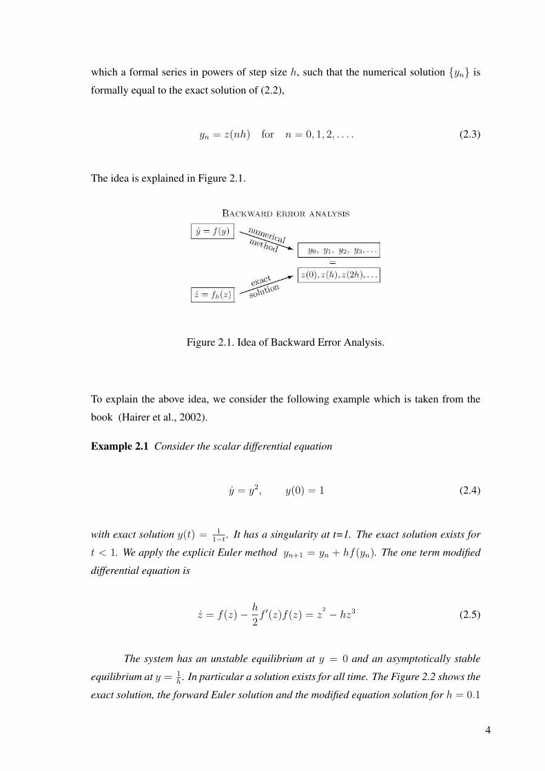
which a formal series in powers of step size h, such that the numerical solution {yn} is

formally equal to the exact solution of (2.2),

yn = z(nh) for n = 0, 1, 2, . . . . (2.3)

The idea is explained in Figure 2.1.

Figure 2.1. Idea of Backward Error Analysis.

To explain the above idea, we consider the following example which is taken from the

book (Hairer et al., 2002).

Example 2.1 Consider the scalar differential equation

y = y2, y(0) = 1 (2.4)

with exact solution y(t) = 11−t

. It has a singularity at t=1. The exact solution exists for

t < 1. We apply the explicit Euler method yn+1 = yn + hf(yn). The one term modified

differential equation is

z = f(z)− h

2f ′(z)f(z) = z

2 − hz3 (2.5)

The system has an unstable equilibrium at y = 0 and an asymptotically stable

equilibrium at y = 1h

. In particular a solution exists for all time. The Figure 2.2 shows the

exact solution, the forward Euler solution and the modified equation solution for h = 0.1

4

The modified equation is not much closer to the numerical solution than the exact solution

is, but it does exist for all time.

Figure 2.2. Exact, forward Euler and 1-term modified equation solutions to y =y2, y(0) = 1.

Continuing the procedure outlined above to determine higher order terms (and

making use of symbolic mathematics software) gives the five term modified equation. Its

output is

z = z2 − hz3 +3

2h2z4 − 8

3h3z5 +

31

6h4z6 − 157

15h5z7 ∓ .... (2.6)

The Figure 2.3 presents the exact solution, the forward Euler method and m-term modified

equations for m = 1, ..., 5 plotted for h = 2.10−2. We see that the modified equation

solutions ’converge’ to the numerical solution very quickly as h become smaller. We

observe an excellent agreement of the numerical solution with the exact solution of the

modified equation.

By the similar way the modified equation with respect to midpoint rule can be

obtained given as below

z = z2 +1

4h2z4 +

1

8h4z6 +

11

192h6z8 +

3

128h8z10 + .... (2.7)

5

Figure 2.3. Exact, forward Euler and m-term modified equation solutions to y =y2, y(0) = 1 with step-size h = 2.10−2.

For the classical Runge-Kutta method of order 4

z = z2 − 1

24h4z6 +

65

576h6z8 − 17

96h7z9 +

19

144h8z10 ∓ .... (2.8)

We observe that the perturbation terms in modified equation are of size O(hp), where p is

the order of the method. This is true in general.

The error estimation committed by backward error analysis is stated in the following

theorem.

Theorem 2.1 Let f(y) be analytic in a complex neighborhood of y0 and that ||f(y)|| ≤M for ||y − y0|| ≤ 2R i.e., for all y of B2R(y0) := {y ∈ Cd; ||y − y0|| ≤ 2R}, let the

coefficients dj(y) of the method be analytic and bounded in BR(y0). If h < h0/4 where

h0 = R/M then there exists N = N(h) (namely N equal to the largest integer satisfying

hN ≤ h0) such that the difference between the numerical solution y1 = φh(y0) and the

6

exact solution ϕN,t(y0) of the truncated modified equation (2.28) satisfies

||φh(y0)− ϕN,h(y0)|| ≤ hγMe−h0/h. (2.9)

Proof See (Hairer et al., 2002). ¤

Note that the local error does not grow exponentially with the time interval as like the

forward error analysis.

2.2. Modifying Numerical Integrators

Backward error analysis is a purely theoretical tool that gives much insight into the

long-term integration with geometric numerical methods. We shall show that by simply

exchanging the roles of the numerical method and the exact solution, it can be turned into

a means for constructing high order integrators that conserve geometric properties over

long times. Let us be more precise: As before, we consider an initial value problem (2.1)

and a numerical integrator. But now we search for a modified differential equation, again

of the form (2.2), such that the numerical solution {zn} of the method applied with step

size h to (2.2) yields formally the exact solution of the original differential equation (2.1),

i.e.,

zn = y(nh) for n = 0, 1, 2, . . . . (2.10)

The idea is explained in Figure 2.4.

7

Figure 2.4. Idea of Modified Differential Equations.

Notice that this modified equation is different from the one considered before.

However, due to the close connection with backward error analysis, all theoretical and

practical results have their analogue in this new context. The modified differential equa-

tion is again an asymptotic series that usually diverges, and its truncation inherits ge-

ometric properties of the exact flow if a suitable integrator is applied. The coefficient

functions fj(z) can be computed recursively by using a formula manipulation program

like MAPLE. This can be done by developing both sides of z(t + h) = Φfh,h(z(t)) into

a series in powers of h, and by comparing their coefficients. Once a few functions fj(z)

are known, the following algorithm suggests itself:

Consider the truncation

z = f[r]h (z) = f(z) + hf2(z) + . . . + hr−1fr(z) (2.11)

of the modified differential equation corresponding to Φf,h(y). Then,

zn+1 = Ψf,h(zn) := Φf[r]h ,h

(zn) (2.12)

defines a numerical method of order r that approximates the solution of (2.1). We call it

modifying integrator, because the vector field f(y) of (2.1) is modified into f[r]h before the

basic integrator is applied.

This is an alternative approach for constructing high order numerical integrators

for ordinary differential equations (classical approaches are multistep, Runge Kutta, Tay-

lor series, extrapolation, composition, and splitting methods). It is particularly interesting

8

in the context of geometric integration because, as known from backward error analy-

sis, the modified differential equation inherits the same structural properties as (2.1) if a

suitable integrator is applied. This basic idea is explained in the following example.

Example 2.2 For the numerical integration of (2.1) considering the midpoint rule

yn+1 = yn + h f

(yn + yn+1

2

). (2.13)

We find the functions fj(y) of the truncated modified vector field with respect to implicit

midpoint rule.

Consider the truncated modified differential equation (2.11)

˙y = f[r]h (y) = f(y) + hf2(y) + ... + hr−1fr(y)︸ ︷︷ ︸

F

(2.14)

and the Taylor expansion of exact solution y(t) for h

y(t + h) = y(t) + hy(t) +h2

2!y(t) +

h3

3!y3(t) + ..., (2.15)

where y = f ′f , y(3) = f ′f ′f + f ′′(f, f) and yn+1 = φf[r]h ,h

(yn) where the method here

is midpoint rule

yn+1 = yn + hF

(yn + yn+1

2

)(2.16)

yn+1 = yn + hF

(yn + yn + hF ( yn+yn+1

2)

2

)(2.17)

yn+1 = yn + hF

(yn +

h

2F

(yn + yn+1

2

))(2.18)

yn+1 = yn + h

[F (yn) +

h

2F

(yn + yn+1

2

)F ′(yn)

+h2

8F 2

(yn + yn+1

2

)F ′′(yn) + ...

](2.19)

yn+1 = yn + hf + h2

[f2 +

1

2ff ′

]

+h3

[f3 +

1

2f2f

′ +1

4f ′f ′f +

1

8f ′′(f, f)

]+ ... (2.20)

9

Now equating the terms of (2.20) to the terms of the exact solution (2.15) and expanding

by Taylor series we get

f2 = 0 (2.21)

f3 =1

12

(− f ′f ′f +

1

2f ′′(f, f)

)(2.22)

f4 = 0 (2.23)

f5 =h4

120

(f ′f ′f ′f ′f − f ′′(f, f ′f ′f) +

1

2f ′′(f ′f, f ′f)

)

+h4

120

(− 1

2f ′f ′f ′′(f, f) + f ′f ′′(f, f ′f)

+1

2f ′′(f, f ′′(f, f))− 1

2f (3)(f, f, f ′f)

)

+h4

80

(− 1

6f ′f (3)(f, f, f) +

1

24f (4)(f, f, f, f)

)(2.24)

Theorem 2.2 Suppose that the method yn+1 = φf,h(yn) is of order p, i.e.,

φf,h(yn) = ϕh(y) + hp+1δp+1(y) + O(hp+2) (2.25)

where ϕt(y) denotes the exact flow of y = f(y), and hp+1δp+1(y) the leading term of the

local truncation error. The modified equation then satisfies

˙y = f(y) + hpfp+1(y) + hp+1fp+2(y) + ..., y(0) = y0 (2.26)

with fp+1(y) = δp+1(y).

Proof The construction of the functions fj(y) (see the beginning of this section) shows

that fj(y) = 0 for 2 ≤ j ≤ p if and only if φf,h(y)− ϕh(y) = O(hp+1).

A first application of the modified equation (2.2) is the existence of an asymptotic

expansion of the global error. Indeed by the nonlinear variation of constants formula, the

difference between its solution y(t) and the solution y(t) of y = f(y) satisfies

y(t)− y(t) = hpep(t) + hp+1(t) + ... (2.27)

10

Since yn = y(nh) + O(hN) for the solution of a truncated modified equation, this proves

the existence of an asymptotic expansion in powers of h for the global error yn − y(nh).

In general, the series (2.2) diverges and the infinite order modified equation does

not exist. Nonetheless, taking a finite number of terms of the series (2.2) yields a trun-

cated modified equation that can still provide a good approximation to the behavior of the

discrete dynamical system.

Consider the truncated modified differential equation

˙y = FN(y), FN(y) = f(y) + hf2(y) + ... + hN−1(y) (2.28)

There exists an optimal value of m, dependent on h and denoted by N for which

the difference between the m-term modified equation and the numerical solution is mini-

mized. N increases like 1/h as h tends to zero, and usually much larger than the order p

of the numerical method. In other words, the modified equations are indeed a useful tool

in understanding numerical methods. ¤

Next, we explain briefly symplecticity and the related theorems, in the next sec-

tion.

2.3. Symplectic Integrators

A first property of Hamiltonian systems is that the Hamiltonian H(q, p) is a first

integral of the system qi = ∂H∂pi

and pi = −∂H∂qi

where H is the Hamiltonian function

(or just the Hamiltonian) of the system. In this section we shall study another important

property: the symplecticity of its flow.

The basic objects to be studied are two-dimensional parallelograms lying in R2d.

We suppose the parallelogram to be spanned by two vectors

ξ =

(ξq

ξp

), η =

(ηq

ηp

)(2.29)

in the (p, q) space (ξq, ξp, ηq, ηp are in Rd) as

P = {tξ + sη | 0 ≤ t ≤ 1, 0 ≤ s ≤ 1}. (2.30)

11

In the case d = 1 we consider the oriented area

Area(P ) = det

(ξq ηq

ξp ηp

)= ξqηp − ξpηq. (2.31)

In higher dimensions, we replace this by the sum of the oriented areas of the projections

of P onto the coordinate planes (pi, qi), i.e., by

ω(ξ, η) :=d∑

i=1

det

(ξqi ηq

i

ξpi ηp

i

)=

d∑i=1

(ξqi η

pi − ξp

i ηqi ). (2.32)

This defines a bilinear map acting on vectors of R2d, which will play a central role for

Hamiltonian system. In matrix notation, this map has the form

ω(ξ, η) = ξT Jη with J =

(0 I

−I 0

)(2.33)

where I is the identity matrix of dimension d (Hairer et al., 2002).

Definition 2.1 A linear mapping A : R2d → R2d is called symplectic if

AT JA = J (2.34)

or, equivalently, if ω(Aξ,Aη) = ω(ξ, η) for all ξ, η ∈ R2d.

We can find it

ω(Aξ, Aη) = (Aξ)T J(Aη) = ξT AT JA︸ ︷︷ ︸ η (since AT JA = J) (2.35)

= ξT Jη = ω(ξ, η) (2.36)

Definition 2.2 A differentiable map g : U → R2d (where U ⊂ R2d is an open set) is

12

called symplectic if the Jacobian matrix g′(q, p) is everywhere symplectic, i.e., if

g′(q, p)T Jg′(q, p) = J or ω(g′(q, p)ξ, g′(q, p)η) = ω(ξ, η). (2.37)

Lemma 2.1 If ψ and ϕ are symplectic maps then ψ ◦ ϕ is symplectic.

Proof Since ψ is symplectic

(ψ′)T Jψ′ = J , similarly (ϕ′)T Jϕ′ = J, (2.38)

by using the equation (2.38), we get

[(ψoϕ)′

]TJ(ψoϕ)′ = (ψ′oϕ′)T J(ψ′oϕ′) = (ϕ′)T o(ψ′)T Jψ′oϕ′ = J. (2.39)

It gives the symplecticity of two maps. ¤

Theorem 2.3 (Poincare 1899). Let H(q, p) be a twice continuously differentiable func-

tion on U ⊂ R2d. Then, for each fixed t, the flow ϕt is a symplectic transformation

wherever it is defined.

Proof Let ϕt be flow of the Hamiltonian system. ϕ′t is a Jacobian matrix of the flow,

then ϕ′t satisfies the variational equation i.e.

d

dtϕ′t = J−1H ′′ϕ′t where H ′′ =

(Hpp Hpq

Hqp Hqq

)is symmetric. (2.40)

Hence

d

dt(ϕ′Tt Jϕ′t) = [J−1H ′′ϕ′t]

T Jϕ′t + ϕ′Tt JJ−1︸ ︷︷ ︸I

H ′′ϕ′t (2.41)

since JJ−1 = I , we get

d

dt(ϕ′Tt Jϕ′t) = ϕ′Tt H ′′T (J−1)T Jϕ′t + ϕ′Tt H ′′ϕ′t (2.42)

13

now, we will use (H ′′)T = H ′′ and (J−1)T J = −I , let us prove it.

JT = −J. (2.43)

By using the equation (2.43), we get

[(J−1)T J

]T= JT · J−1 = −J · J−1 = −I, (2.44)

then we finally find (J−1)T J = −I . We put (J−1)T J = −I in the last equation

d

dt(ϕ′Tt Jϕ′t) = −ϕ′Tt H ′′ϕ′t + ϕ′Tt H ′′ϕ′t = 0. (2.45)

Since ddt

(ϕ′Tt Jϕ′t) = 0 then ϕ′Tt Jϕ′t = C. When t = 0, we have ϕ′t(t0) = I ⇒ C = J . ¤

Theorem 2.4 Let f : U → R2d be continuously differentiable. Then, y = f(y) is locally

Hamiltonian if and only if its flow ϕt(y) is symplectic for all y ∈ U and for all sufficiently

small t.

Proof Assume that the flow ϕt is symplectic, and we have to prove the local existence

of a function H(y) such that f(y) = J−1∇H(y). Using the fact that ∂ϕt

∂y0is a solution of

the variational equation Ψ = f ′(ϕt(y0))Ψ, we obtain

d

dt

((∂ϕt

∂y0

)T

J(∂ϕt

∂y0

))=

(∂ϕt

∂y0

)(f ′(ϕt(y0))

T J + Jf ′(ϕt(y0))(∂ϕt

∂y0

)= 0. (2.46)

Putting t = 0, it follows from J = −JT that Jf ′(y0) is a symmetric matrix for all y0. ¤

Definition 2.3 A numerical one-step method is called symplectic if the one-step map y1 =

Φh(y0) is symplectic whenever it is applied to a smooth Hamiltonian system. If the method

is symplectic, we have

Φ′h(y)T J Φ′

h(y) = J (2.47)

14

where J =

(0 I

−I 0

).

2.3.1. Examples of the Symplectic Methods

One of the example of symplectic method is implicit midpoint method.

Example 2.3 The implicit midpoint rule is symplectic.

Proof The second order implicit midpoint rule is given as

Un+1 = Un + hf(Un + Un+1

2

). (2.48)

Consider the Hamiltonian problem of the form

y = J−1∇H(y) (2.49)

The application of the midpoint rule to the Hamiltonian system in (Hairer et al., 2002)

yields

Un+1 = Un + hJ−1∇H(Un + Un+1

2

)(2.50)

Suppose Un+1 = ψn(Un), then we need to show

ψ′Tn Jψ′n = J. (2.51)

First compute ψ′n as follows

ψ′n =∂Un+1

∂Un

= I + hJ−1H ′′(Un + Un+1

2

)(1

2

)(∂Un+1

∂Un

+ I)

(2.52)

=(I − h

2J−1H ′′

)−1(I +

h

2J−1H ′′

)(2.53)

15

Next, the symplecticity condition (2.51) can be written as

(I +

h

2J−1H ′′

)J(I +

h

2J−1H ′′

)T

=(I − h

2J−1H ′′

)J(I − h

2J−1H ′′

)T

. (2.54)

By using the equalities (H ′′)T = H ′′ (since H is symmetric) and (J−1)T = −J−1 = J ,

we get

(I +

h

2J−1H ′′

)T

= I − h

2H ′′J−1,

(I − h

2J−1H ′′

)T

= I +h

2H ′′J−1. (2.55)

Inserting this into the equation (2.54), we get

(IJ +

h

2J−1H ′′J

)(I − h

2H ′′J−1

)=

(IJ − h

2J−1H ′′J

)(I +

h

2H ′′J−1

). (2.56)

After some manipulations of equation (2.56), we have

J +h

2J−1H ′′J − h

2JH ′′J−1 − h2

4J−1H ′′JH ′′J−1 = J +

h

2JH ′′J−1

−h

2J−1H ′′J − h2

4J−1H ′′JH ′′J−1 (2.57)

Finally, equation (2.57) implies the following result

hJH ′′J−1 = hJ−1H ′′J (2.58)

Since J−1 = −J then −JH ′′J = −JH ′′J completes the proof. ¤

The next example of symplectic method of order 1 is so-called symplectic method. If the

partitioned Euler method is applied to the Hamiltonian system, the obtained method is

called symplectic Euler method. Next example proves that symplectic euler method is a

symplectic method.

16

Example 2.4 The so-called symplectic Euler method

un+1 = un − h∂H

∂v(un+1, vn), vn+1 = vn + h

∂H

∂u(un+1, vn) (2.59)

is a symplectic method of order 1.

Proof Differentiation of (2.59) with respect to (un, vn) yields

(I + hHT

vu 0

−hHuu I

)(∂(un+1, vn+1)

∂(un, vn)

)=

(I −hHvv

0 I + hHvu

)(2.60)

where the matrices Hvu, Huu, . . . of partial derivatives are all evaluated at (un+1, vn). This

relation allows us to compute ∂(un+1,vn+1)∂(un,vn)

and to check in a straightforward way the sym-

plecticity condition

∂(un+1, vn+1)

∂(un, vn)

T

J∂(un+1, vn+1)

∂(un, vn)= J. (2.61)

The same proof shows that the adjoint method of (2.59),

un+1 = un − h∂H

∂v(un, vn+1), vn+1 = vn + h

∂H

∂u(un, vn+1) (2.62)

is also symplectic. ¤

In the next section, we briefly explain the geometric properties which preserve by this

construction.

2.4. Geometric Properties

The importance of backward error analysis in the context of geometric numerical

integration lies in the fact that properties of numerical integrators are transferred to cor-

responding properties of modified equations.Because of the close relationship between

backward error analysis and the approach of modifying integrators, it is not a surprise

that most results can be extended to our situation. The most important properties of the

17

modified equation can be collected given as below:

• If the numerical integrator Φf,h(y) has order p, i.e., the local error satisfies Φf,h(y)−ϕf,h(y) = O(hp+1), then we have fj = 0 for j = 2, ..., p.

• If the numerical integrator Φf,h(y) is symmetric, i.e, Φf,−h(y) = Φ−1f,h(y), then the

modified differential equation has an expansion in even powers of h, i.e., f2j = 0

for all j, and modifying integrator is symmetric.

• If the basic method Φf,h(y) exactly conserves a first integral I(y) of (2.1), then the

modified differential equation has I(y) as first integral, and the modifying integrator

exactly conserves I(y).

• If the basic method is symplectic for Hamiltonian systems of the form

y = J−1∇H(y), (2.63)

the modifying integrator is also symplectic.

• If the basic method is reversible for reversible differential equations then the modi-

fied differential equation and the modifying integrator are reversible.

The proofs of these properties can be found in (Hairer et al., 2002). Here we are

not concerned with these proofs.

In the next chapter, after giving a brief introduction about the symplecticity and

examples of symplectic methods, we will construct a higher order symplectic methods by

using modified vector field idea based on the Lobatto IIIA-IIIB method of order 2.

18

CHAPTER 3

CONSTRUCTION OF LOBATTO METHOD

We consider the initial value problem

y = f(y), y(0) = y0 (3.1)

and a numerical one-step integrator yn+1 = Φf,h(yn). We search for a modified differen-

tial equation

z = fh(z) = f(z) + hf2(z) + h2f3(z) + ..., z(0) = y0 (3.2)

such that the numerical solution {zn} of the method applied with step size h to (3.2) yields

formally the exact solution of the original differential equation (3.1), i.e. zn = y(nh) for

n = 0, 1, 2, ... The coefficient functions fj(z) can be computed recursively.

Having found first functions fj(z), one can use the truncation

z = f[r]h (z) = f(z) + hf2(z) + ... + hr−1fr(z) (3.3)

of the modified differential equation corresponding to Φf,h(y). A numerical method

zn+1 = Φf[r]h ,h

(zn) approximates the solution of (3.1) with order r. It is called a mod-

ifying integrator because it applies to the modified vector field f[r]h instead of f(y).

We will consider partitioned systems

{y′ = f(y, z)

z′ = g(y, z)(3.4)

19

and separable systems

{y′ = f(z)

z′ = g(y)(3.5)

In particular, we will be interested in canonical Hamiltonian equations, which are

generated by a Hamiltonian function H(y, z):

f(y, z) = Hz(y, z), g(y, z) = −Hy(y, z). (3.6)

Compact form of Hamiltonian system is given by where such system often arise in me-

chanical systems described by a Hamiltonian function

H =p2

2+ V (q) (3.7)

which provides us

{q′ = p

p′ = −Vq(q).(3.8)

with the Hamiltonian equations of motion.

3.1. Partitioned Runge-Kutta Methods

In this section we consider differential equations in the partitioned form

y = f(y, z), z = g(y, z), (3.9)

where the variables y and z may be vectors of different dimensions.

The idea is to take two different Runge-Kutta methods, and to treat the y-variables

with the first method (aij, bi), and the z-variables with the second method (aij, bi).

20

Definition 3.1 Let bi,aij and bi,aij be the coefficients of two Runge-Kutta methods. A

partitioned Runge-Kutta method for the solution of y = f(y, z) and z = g(y, z) are given

by

ki = f

(y0 + h

s∑j=1

aijkj, z0 + h

s∑j=1

aijlj

), (3.10)

li = g

(y0 + h

s∑j=1

aijkj, z0 + h

s∑j=1

aijlj

), (3.11)

y1 = y0 + h

s∑i=1

biki, z1 = z0 + h

s∑i=1

bili. (3.12)

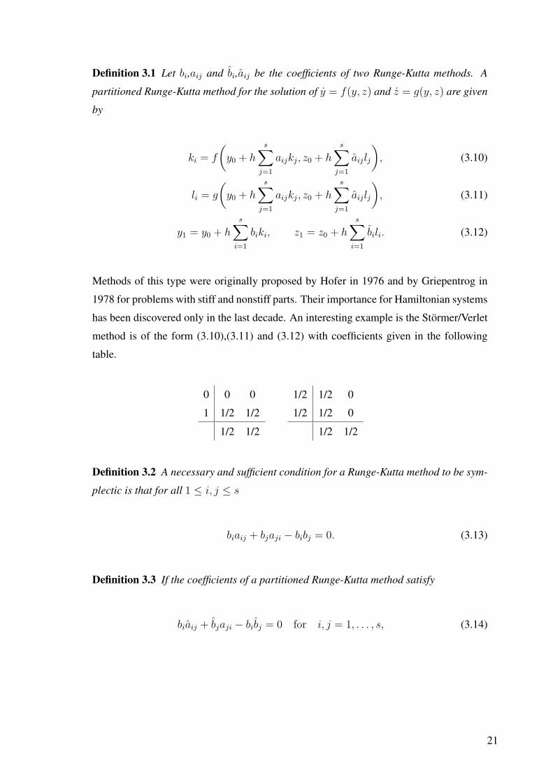
Methods of this type were originally proposed by Hofer in 1976 and by Griepentrog in

1978 for problems with stiff and nonstiff parts. Their importance for Hamiltonian systems

has been discovered only in the last decade. An interesting example is the Stormer/Verlet

method is of the form (3.10),(3.11) and (3.12) with coefficients given in the following

table.

0 0 0

1 1/2 1/2

1/2 1/2

1/2 1/2 0

1/2 1/2 0

1/2 1/2

Definition 3.2 A necessary and sufficient condition for a Runge-Kutta method to be sym-

plectic is that for all 1 ≤ i, j ≤ s

biaij + bjaji − bibj = 0. (3.13)

Definition 3.3 If the coefficients of a partitioned Runge-Kutta method satisfy

biaij + bjaji − bibj = 0 for i, j = 1, . . . , s, (3.14)

21

and the following condition

bi = bi for i = 1, . . . , s, (3.15)

then it is symplectic.

If the Hamiltonian is of the form H(p, q) = T (p) + U(q), i.e., it is separable, then

the condition (3.14) alone implies the symplecticity of the numerical flow.

3.2. Lobatto IIIA - IIIB Pairs

In this part of thesis we will construct higher order method corresponding to Lo-

batto IIIA-IIIB pair of method.

Definition 3.4 The partitioned Runge-Kutta method composed of the s-stage Lobatto IIIA

and the s-stage Lobatto IIIB method, is of order 2s-2.

Lobatto IIIA - IIIB pair of order 2 is given as follows:

k1 = f

(y0, z0 +

h

2l1

), k2 = f

(y0 +

h

2(k1 + k2), z0 +

h

2l1

), (3.16)

l1 = g

(y0, z0 +

h

2l1

), l2 = g

(y0 +

h

2(k1 + k2), z0 +

h

2l1

), (3.17)

y1 = y0 +h

2(k1 + k2), (3.18)

z1 = z0 +h

2(l1 + l2). (3.19)

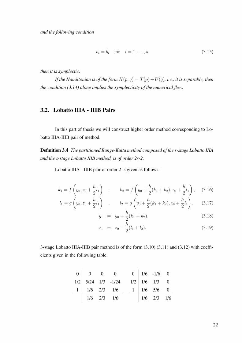
3-stage Lobatto IIIA-IIIB pair method is of the form (3.10),(3.11) and (3.12) with coeffi-

cients given in the following table.

0 0 0 0

1/2 5/24 1/3 -1/24

1 1/6 2/3 1/6

1/6 2/3 1/6

0 1/6 -1/6 0

1/2 1/6 1/3 0

1 1/6 5/6 0

1/6 2/3 1/6

22

The Definition (3.1) together with the coefficients of 3-stage Lobatto IIIA-IIIB pair method

given in the above table yields the Lobatto IIIA-IIIB method of order 4 are given by

k1 = f(y0, z0 +h

6(l1 − l2)), (3.20)

k2 = f(y0 +h

24(5k1 + 8k2 − k3), z0 +

h

6(l1 + 2l2)), (3.21)

k3 = f(y0 +h

6(k1 + 4k2 + k3), z0 +

h

6(l1 + 5l2)), (3.22)

l1 = g(y0, z0 +h

6(l1 − l2)), (3.23)

l2 = g(y0 +h

24(5k1 + 8k2 − k3), z0 +

h

6(l1 + 2l2)), (3.24)

l3 = g(y0 +h

6(k1 + 4k2 + k3), z0 +

h

6(l1 + 5l2)), (3.25)

y1 = y0 +h

6(k1 + 4k2 + k3), z1 = z0 +

h

6(l1 + 4l2 + l3). (3.26)

In the next section, we will construct a new fourth order modified Lobatto method. We

will compare the method given in (3.26) with the new proposed method in the computa-

tional part.

3.3. Modified Lobatto Methods

We consider the modified differential equations which have the perturbated form

given by

{y′ = f(y, z) + h2a(y, z),

z′ = g(y, z) + h2b(y, z).(3.27)

Our aim is to determine the functions a(y, z) and b(y, z). We simply follow the below

procedures. The Taylor expansion of the exact solution of y for a fixed t is

y1 = y(t + h) = y(t) + hy′(t) +h2

2!y′′(t) +

h3

3!y′′′(t) +

h4

4!y′′′′(t) + . . . . (3.28)

23

Derivatives in the equation (3.28) for equation (3.4) are given by

y′ = f (3.29)

y′′ = fyf + fzg (3.30)

y′′′ =(fyyf + fyzg

)f + fy

(fyf + fzg

)

+(fyzf + fzzg

)g + fz

(gyf + gzg

)(3.31)

= 2fyz(f, g) + fyy(f, f) + fyfyf + fyfzg + fzz(g, g)

+fzgyf + fzgzg (3.32)

y′′′′ =[(fyyyf + fyyzg)f + fyy(fyf + fzg) + (fyyzf + fyzzg)g + fyz(gyf + gzg)

]f

+2(fyf + fzg)(fyyf + fyzg) +[(fyyf + fyzg)f + (fyf + fzg)fy

+(fyzf + fzzg)g + fz(gyf + gzg)]fy + . . . (3.33)

Using Taylor series expansion and substituting (3.33) into (3.28), in equation (3.18), y1

can be found as

y1 = y(t + h) = y + hf +h2

2(fyf + fzg) +

h3

6

(2fyz(f, g)

+fyy(f, f) + fyfyf + fyfzg + fzz(g, g) + fzgyf + fzgzg)

+h4

24y′′′′. (3.34)

Next, the Lobatto method of order 2 to modified differential equation leads to below

equation

y0 +h

2(k1 + k2) = y +

h

2

[2f + h

(fyf + fz(g + h2b)

)+

(h

2

)2

(fzz(g, g) + 2(fyz(f, g) + fyy(f, f) + fyfyf

+fyfzg + fzgzg))

+ . . . + h2[2a + ayhf + azhg]

]. (3.35)

24

Finally, we compare the terms of (3.34) and (3.35) with respect to the powers of h,

1

6

(2fyz(f, g) + fyy(f, f) + fyfyf + fyfzg + fzz(g, g) + fzgyf + fzgzg

)=

1

4

(fyz(f, g) + fyy(f, f) + fyfyf + fyfzg +

1

2fzz(g, g) + fzgzg

)+ a(y, z) (3.36)

we get

a(y, z) =1

12

(− fyy(f, f) + fyz(f, g) +

1

2fzz(g, g)

−fyfyf − fyfzg + 2fzgyf − fzgzg

)(3.37)

By the same procedure we can obtain the function b(y, z) given by

b(y, z) =1

12

(− gyy(f, f) + gyz(f, g) +

1

2gzz(g, g)

−gyfyf − gyfzg + 2gzgyf − gzgzg

)(3.38)

If the original equations are Hamiltonian, then the modified differential equations (3.27)

are generated by the Hamiltonian function

H [3] = H +h2

12

(−Hyy(f, f) + Hyz(f, g) +

1

2Hzz(g, g)

), (3.39)

where f and g are given by (3.6).

So far the calculations of the coefficient functions for the modified equations are

more complex for the systems introduced in equation (3.27). So we choose separable

systems after this section since the calculations of the coefficient functions become more

easier. For separable systems the modified differential equations are

{y′ = f(z) + h2a(y, z),

z′ = g(y) + h2b(y, z),(3.40)

25

where fy ≡ 0 and gz ≡ 0. Taking the derivatives of original system, for y we get

y′ = f(z) (3.41)

y′′ = fzg (3.42)

y′′′ = fzz(g, g) + fzgyf (3.43)

y′′′′ =(fzzz(g, g, g) + 2fzz(gyf, g)

)

+(fzz(gyf, g) + fzgyy(f, f) + fzgyfzg

)(3.44)

for z we get

z′ = g(y) (3.45)

z′′ = gyf (3.46)

z′′′ = gyy(f, f) + gyfzg (3.47)

z′′′′ =(gyyy(f, f, f) + 2gyy(fzg, f)

)

+(gyy(fzg, f) + gyfzz(g, g) + gyfzgyf

). (3.48)

Applying the third order approximation to k1, k2, l1 and l2, we have

k1 = f +h

2fz(g + h2b) +

1

2

(h

2

)2

fzz(g, g)

+1

6

(h

2

)3

(g, g, g) + h2[a + az

h

2g]

+O(h4) (3.49)

and k2 as follows

k2 = f +h

2fz(g + h2b) +

1

2

(h

2

)2

fzz(g, g)

+1

6

(h

2

)3

(g, g, g) + h2[a + ayhf + az

h

2g]

+O(h4) (3.50)

l1 = g + h2[b + bz

h

2g]

+O(h4) (3.51)

26

and l2 as follows

l2 = g +h

2gy

[2f + hfzg +

(h

2

)2

fzz(g, g) + h2a]

+1

2

(h

2

)2

gyy(2f + hfzg, 2f + hfzg)

+1

6

(h

2

)3

gyyy(2f, 2f, 2f) + h2[b + byhf + bz

h

2g]

+O(h4) (3.52)

Putting k1 and k2 into (3.18),

y0 +h

2(k1 + k2) = y +

h

2

[2f + 2

(h

2

)fz(g + h2b) +

(h

2

)2

fzz(g, g)

+1

3

(h

2

)3

fzzz(g, g, g) + h2(2a + ayhf + azhg)]

+O(h5) (3.53)

and (3.41) into y1,

y1 = y + hf +1

2h2fzg +

1

6h3[fzz(g, g) + fzgyf ] +

1

24h4

[fzzz(g, g, g) + 3fzz(gyf, g) + fzgyy(f, f) + fzgyfzg] (3.54)

Since (3.53) is equal to (3.54), a(y, z) can be found easily.

a(y, z) =1

12

(1

2fzz(g, g) + 2fzgyf

). (3.55)

Secondly, we put l1 and l2 into (3.19),

z0 +h

2(l1 + l2) = z +

h

2

[2g + 2

(h

2

)gy2f +

(h

2

)gyhfzg

+(h

2

)3

gyfzz(g, g) +(h

2

)gyah2 +

h2

2gyy(f, f) +

h3

2gyy(f, fzg)

+h3

6gy,y,y(f, f, f) + h2(2b + byhf + bzhg)

]+O(h5) (3.56)

27

and (3.45) into z1,

z1 = z + hg +1

2h2gyf +

1

6h3[gyy(f, f) + gyfzg] +

1

24h4

[gyyy(f, f, f) + 3gyy(fzg, f) + gyfzz(g, g) + gyfzgyf ] (3.57)

Since (3.56) is equal to (3.57), b(y, z) can be found easily as follows;

b(y, z) = − 1

12(gyy(f, f) + gyfzg). (3.58)

If the original equations are Hamiltonian, the modified differential equations are generated

by

H [3] = H +h2

12

(−Hyy(f, f) +

1

2Hzz(g, g)

). (3.59)

For mechanical system, equation (3.8) can read as

H [3] = H +h2

12

(−Vqq(p, p) +

1

2(Vq, Vq)

). (3.60)

Applying (3.55) and (3.58) into mechanical system

H =1

2p2 + V (q) (3.61)

where q = f(p) = p, p = g(q) = −V (q), we get

a =1

6gqp, b = − 1

12gqq(p, p)− 1

12gqg. (3.62)

The modified differential equations for separable systems are

{q′ = f(p) + h2a(q, p),

p′ = g(q) + h2b(q, p),(3.63)

28

so the modified equations then take the following form

q′ = p +h2

6gqp =

(I − h2

6Vqq

)p

p′ = −Vq(q)− h2

12(gqq(p, p) + gqg).

(3.64)

After applying Lobatto IIIA - IIIB pair method of order 2 to (3.64), k1, k2, l1 and l2 can

be given as follows

k1 =

(I +

h2

6gq(q0)

)(p0 +

h

2l1

), (3.65)

k2 =

(I +

h2

6gq(q1)

)(p0 +

h

2l1

), (3.66)

l1 = g(q0)− h2

12

(gqq(q0)

(p0 +

h

2l1, p0 +

h

2l1

)+ gq(q0)g(q0)

), (3.67)

l2 = g(q1)− h2

12

(gqq(q1)

(p0 +

h

2l1, p0 +

h

2l1

)+ gq(q1)g(q1)

). (3.68)

Combining the above equations with (3.18) and (3.19), we have

q1 = q0 + h

(I +

h2

12(gq(q0) + gq(q1))

)(p0 +

h

2l1

), (3.69)

p1 = p0 +h

2

(g(q0) + g(q1)− h2

12

[gqq(q0)(p0 +

h

2l1, p0 +

h

2l1)

+gqq(q1)(p0 +h

2l1, p0 +

h

2l1) + gq(q0)g(q0) + gq(q1)g(q1)

]). (3.70)

these equations leads to a scheme which can be split into three stages:

p1/2 = p0 +h

2

(g(q0)− h2

12

(gqq(q0)(p1/2, p1/2) + gq(q0)g(q0)

)), (3.71)

q1 = q0 + h

(I +

h2

12(gq(q0) + gq(q1))

)p1/2, (3.72)

p1 = p1/2 +h

2

(g(q1)− h2

12

(gqq(q1)(p1/2, p1/2) + gq(q1)g(q1)

)), (3.73)

29

where we introduced an intermediate variable

p1/2 = p0 +h

2l1. (3.74)

The equations (3.71) and (3.72) are implicit, the equation (3.73) is explicit.

30

CHAPTER 4

CONVERGENCE ANALYSIS

In this chapter after presenting the new numerical method, its convergence proper-

ties are analyzed using concepts familiar from numerical analysis of stability, consistency

and order.

Definition 4.1 Consistency and order: Suppose the numerical method is

yn+k = φ(tn+k; yn, yn+1, ..., yn+k−1; h). (4.1)

The local error of the method is the error committed by one step of the method. That is, it

is the difference between the result given by the method, assuming that no error is made

in earlier steps, and the exact solution:

δhn+k = φ(tn+k; y(tn), y(tn+1), ..., y(tn+k−1); h)− y(tn+k). (4.2)

The method is said to be consistent if

limh→0

δhn+k

h= 0. (4.3)

The method has order p if

δhn+k = O(hp+1) as h → 0. (4.4)

Hence a method is consistent if it has an order greater than 0. Most methods being used

in practice attain higher order. Consistency is a necessary condition for convergence, but

not sufficient; for a method to be convergent, it must be both consistent and stable.

A related concept is the global error, the error sustained in all the steps one needs

to reach a fixed time t. Explicitly, the global error at time t is yN−y(t) with N = (t−t0)/h

31

where N is the number of the discretization points and yN , y(t) represents the numerical

solution and exact solution, respectively. The global error of a pth order one-step method

isO(hp); in particular, such a method is convergent. This statement is not necessarily true

for multi-step methods.

Proposition 4.1 Application of the Lobatto IIIA - IIIB pair of the second order to the

modified differential equations gives a numerical method of order 4.

Proof For simplicity, we prove the theorem for mechanical system given by

q = p (4.5)

p = −Vq(q). (4.6)

The application of Lobatto IIIA-IIIB pair method given in (3.16),(3.17),(3.18) and (3.19)

to the above mechanical system yields

q′ = p +h2

6gqp =

(I − h2

6Vqq

)p

p′ = −Vq(q)− h2

12(gqq(p, p) + gqg).

(4.7)

Traditionally, local error analysis is done by comparing the Taylor expansions of exact

solution and the numerical solution.

For one-step method it is useful to write these expansions in the form. The Taylor

expansion of k1, k2, l1, l2 around the (q0, p0) are given in the below equations. For k1, we

have

k1 = f(q0, p0) +h

2l1

∂f

∂p(q0, p0) +

h2

2!l21

∂2f

∂p2(q0, p0) + ... (4.8)

= (p0 +h

2l1)(1− h2

6gq) +

h

2l1fp +

h2

4l21

∂2f

∂p2(q0, p0)

︸ ︷︷ ︸0

+... (4.9)

= p0 − h2

6gqp0 +

h

2l1 − h3

12l1gq +

h

2l1(1− h2

6gq) (4.10)

= p0 − h2

6gqp0 + hl1 − h3

6l1gq (4.11)

32

For l1, we have

l1 = g(q0, p0 +h

2l1) = g(q0, p0) +

h

2l1gq +

h2

4l21gqq + ... (4.12)

= −Vq(q0)− h2

12(gqq(p0, p0) + gqg) +

h

2l1[−Vqq(q0)

−h2

12(gqqq(p0, p0) + gqqg + g2

q )] + ... (4.13)

Since we will use the below equation which q1 and q0 are related in the next step

q1 = q0 +h

2(k1 + k2). (4.14)

Inserting k1 and k2 (k1 = k2) into (4.14), we get

q1 = q0 +h

2(k1 + k2) = q0 + hp0 − h3

6gqp0 + h2l1 − h4

6l1gq. (4.15)

= q0 + hp0 − h3

6gqp0 + h2(−Vq(q0)− h2

12gqq(p0, p0)− h2

12gqg + ...)

−h4

6(−Vq(q0)− h2

12gqq(p0, p0)− h2

12gqg + ...)gq. (4.16)

The Taylor expansion of the exact solution around the point t0 is

q(t0 + h) = q(t0) + hq(t0) +h2

2!q(t0) +

h3

3!q(3)(t0) +

h4

4!q(4)(t0) + ... (4.17)

Next, we compute the derivatives of q in the Taylor expansion and substitute these deriva-

tives into the equation (4.17), then the exact solution of

q = p +h2

6gqp (4.18)

33

is

q(t0 + h) = q0 + h(p0 − h2

6gqp0) +

h2

2!(−Vq(q0)− h2

6gqq − h2

6gqg)

+h3

3!(−h2

6gqqq − ...) +

h4

4!(Vq(q0) +

h2

3gqqgq +

h2

3g2

qg) + ... (4.19)

Substracting q1 from q(t0 + h), we get

h3

3!(−h2

6gqqq − ...) = C1h

5 (4.20)

This completes first part of proof.

For the second part of proof, we expand l1 around (q0, p0),

l1 = g(q0, p0 +h

2l1) = g(q0, p0) +

h

2l1gq +

h2

4l21gqq + ... (4.21)

= −Vq(q0)− h2

12(gqq(p0, p0) + gqg) +

h

2l1[−Vqq(q0)

−h2

12(gqqq(p0, p0) + gqqg + g2

q )] + ... ∼= g (4.22)

= −Vq(q0)− h2

12(gqq(p0, p0) + gqg) +

h

2g[−Vqq(q0)

−h2

12(gqqq(p0, p0) + gqqg + g2

q )] +h2

4g2gqq + ... (4.23)

= −Vq(q0)− h2

12gqq(p0, p0)− h2

12gqg − h

2gVqq(q0)

−h3

24gqqqg − h3

24gqqg

2 − h3

24g2

qg +h2

4g2gqq + ... (4.24)

and

l2 = g(q0 +h

2(k1 + k2), p0 +

h

2l1) (4.25)

= −Vq(q0 + hp0 − h3

6gqp0 + h2g − h4

6gqg)− h2

12(gqq(p0, p0) + gqg)

+h

2ggq +

h2

4g2gqq + ... (4.26)

34

Since we will use the relation in the next step where q1 and q0 related with the below

equation

p1 = p0 +h

2(l1 + l2) (4.27)

Inserting l1 and l2 into (4.27), we get

= p0 − hVq(q0)− h3

12gqq(p0, p0)− h3

12gqg − h2

2Vqq(q0)

−h4

24gqqq(p0, p0)− h4

24gqqg − h4

24g2

q −h3

6Vqqq + ... (4.28)

Next, we compute the derivatives of p in the (4.17) and substitute these derivatives into

the equation (4.17). The exact solution of

p = −Vq(q)− h2

12(gqq(p, p) + gqg) (4.29)

is

p(t0 + h) = p0 + h(−Vq(q0)− h2

12gqq(p0, p0)− h2

12gqg)

+h2

2!(−Vqq(q0)− h2

12gqqq(p0, p0)− h2

12gqqg − h2

12g2

q )

+h3

3!(−Vqqq(q0, q0)− h2

12gqqqq − h2

12gqqqg − h2

12gqqgq − ...)

+h4

4!... (4.30)

Substracting p1 from p(t0 + h), we get

h3

3!(−h2

12gqqqq − h2

12gqqqg − h2

12gqqgq − ...) = C2h

5, (4.31)

and this completes second part of proof.

35

Therefore the difference between exact and numerical solution are estimated by

‖q(t0 + h)− q1‖ ≤ C1h5 (4.32)

and

‖p(t0 + h)− p1‖ ≤ C2h5. (4.33)

This inequality shows that the method is order four. Above inequality leads to the follow-

ing corollary. ¤

Corollary 4.1 The modified Lobatto method is consistent.

Proof The consistency of the method is obvious since limh→0Tn+1

h= 0 where Tn+1 is

truncation error of the method. ¤

Next, the theoretical findings are proven by the numerical test problem.

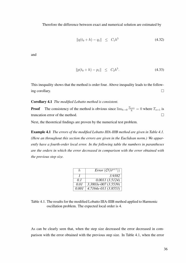
Example 4.1 The errors of the modified Lobatto IIIA-IIIB method are given in Table 4.1.

(Here an throughout this section the errors are given in the Euclidean norm.) We appar-

ently have a fourth-order local error. In the following table the numbers in parantheses

are the orders in which the error decreased in comparison with the error obtained with

the previous step size.

h Error (O(hp+1))

1 3.93820.1 0.0011 (3.5124)

0.01 3.3803e-007 (3.5539)0.001 4.7164e-011 (3.8553)

Table 4.1. The results for the modified Lobatto IIIA-IIIB method applied to Harmonicoscillation problem. The expected local order is 4.

As can be clearly seen that, when the step size decreased the error decreased in com-

parison with the error obtained with the previous step size. In Table 4.1, when the error

36

decreased we got more regular results about the order of the modified Lobatto IIIA-IIIB

method.

4.1. Stability Analysis

In this section we present the stability analysis for the new higher order symplectic

methods which where constructed in the previous chapter.

So far we have examined stability theory only in the context of a scalar differential

equation y′(t) = f(y(t)) for a scalar function y(t). In this section we will look at how

this stability theory carries over to systems of m differential equations where y(t) ∈ Rm.

For a linear system y′ = Ay, where A is m × m matrix, the solution can be written as

y(t) = eAty(0) and the behavior is largely governed by the eigenvalues of A. A necessary

condition for stability is that hλ be in the stability region for each eigenvalue of A. For

general nonlinear systems y′ = f(y), the theory is more complicated, but a good rule

of thumb is that hλ should be in the stability region for each eigenvalue of the Jacobian

matrix f ′(y). This may not be true if the Jacobian is rapidly changing with time, or even

for constant coefficient linear problems in some highly nonnormal cases, but most of the

time eigenanalysis is surprisingly effective.

Clearly the one-dimensional test equation

y′(t) = λy(t), λ ∈ C, Re(λ) < 0, t ∈ [0,∞) (4.34)

is not suitable for the study of absolute stability of partitioned discretization methods as

we emphasized in the previous subsection. Since we study mainly on separable systems

we have to determine the stability condition of the new proposed methods applied to such

systems.

Proposition 4.2 The new symplectic methods applied to the separable systems given in

(3.5) with test equations

q = αp (4.35)

p = βq (4.36)

37

that leads to the mapping yn+1 = R(h)yn said to be stable if |Tr(R)| < 2 where R(h) is

the linear stability matrix depending on the coefficients α,β and the time-step h.

Proof We have the equation in the form

d

dty = Ay, (4.37)

where

A =

(0 α

β 0

). (4.38)

The application of the new method leads to the mapping

yn+1 = R(h)yn. (4.39)

Consider the 2× 2 matrix R(h) such that

R(h) =

(a11 a12

a21 a22

). (4.40)

A sufficient condition for stability is that the eigenvalues of method are (i) in the unit disc

in the complex plane, and (ii) simple (not repeated) if on the unit circle. Since R(h) is a

symplectic map one of its properties is that its determinant is equal to 1.

The eigenvalues of the transformation are given by the characteristic equation

det

(a11 − λ a12

a21 a22 − λ

)= ((a11 − λ)(a22 − λ))− a12a21 = 0 (4.41)

= λ2 − (a11 + a22)︸ ︷︷ ︸Tr(R)

λ + a11a22 − a12a21︸ ︷︷ ︸det(R)=1

= 0 (4.42)

= λ2 − Tr(R)λ + 1 = 0. (4.43)

The eigenvalues of R are solutions of λ2 − Tr(R)λ + 1 = 0.

38

Following Arnold’s treatment of the stability of symplectic maps ( Olver, 1993),

if the two roots λ1 and λ2, of this equation are complex conjugates then

λ =Tr(R)

2± i

√1− (Tr(R)

2

)2. (4.44)

For stability λ < 1, hence |Tr(R)| < 2 is required. Because the norms of the eigenvalues

given in the equation (4.39) are 1 it means that the roots are on the unit circle. For the

stability condition the roots can not be multiple if they are on the unit circle. Since R

depends explicitly on the step-size h, it is necessary to take the least positive solution of

|Tr(R)| = 2 with respect to h in the calculation of stability criteria. ¤Since the general form of the Hamiltonian system is

q = αp (4.45)

p = βq. (4.46)

Applying (4.45) and (4.46) to mechanical system given by the equations (3.16),(3.17),(3.18)

and (3.19),

q′ = p +h2

6gqp =

(I − h2

6Vqq

)p

p′ = −Vq(q)− h2

12(gqq(p, p) + gqg),

(4.47)

we obtain the modified differential equations of the system (4.45) and (4.46) in the form

q′ = αp

(1− h2

6

)(4.48)

p′ = βq

(1 +

h2

12

). (4.49)

Next proposition asserts the stability condition for the mechanical system.

Proposition 4.3 The modified Lobatto method applied to the system (4.48) and (4.49) is

stable for∣∣∣∣2 + h2αβ − h4

8αβ − h6

72αβ

∣∣∣∣ < 2.

39

Proof Applying (4.45) and (4.46) to the mechanical system, we get (4.48) and (4.49).

Taking h = h2

12, the modified system given in equations (4.48),(4.49) takes the form

q′ = αp(1− 2h), p′ = βq(1 + h). (4.50)

The application of the Lobatto IIIA-IIIB given in (3.16),(3.17),(3.18) and (3.19) yields

expressions k1,k2,

k1 = k2 = f(q0, p0 +h

2l1) =

[α(p0 +

h

2(βq0(1 + h))

)](1− 2h

)(4.51)

and l1,l2 below

l1 = βq0(1 + h), l2 =

{β

[q0 + h

(α(p0 +

h

2(βq0(1 + h)))

)(1− 2h

)]}

(1 + h

)(4.52)

Since

qn+1 = qn +h

2(k1 + k2), pn+1 = pn +

h

2(l1 + l2), (4.53)

then

qn+1 = qn + h

[(α(pn +

h

2(βqn(1 + h)))

)(1− 2h)

], (4.54)

pn+1 = pn +h

2

{βqn(1 + h) +

[β(qn + h(α(pn

+h

2(βqn(1 + h))))(1− 2h)

)(1 + h

)]}

. (4.55)

40

As a result,

qn+1 = qn

(1 +

h2

2αβ − h2h

2αβ − h2h2αβ

)+ pn

(hα− 2hhα

), (4.56)

pn+1 = pn

(1 +

h2

2αβ − h2hαβ − h2h2αβ

)

+qn

(hβ − 3

4h3h2αβ2 + hhβ +

h3

4αβ2 +

h2h

2αβ − h3h3

2αβ2

)(4.57)

Matrix form of our modified system is in the form Xn+1 = WXn:

[qn+1

pn+1

]=

[1 + h2

2αβ − h2h

2αβ − h2h2αβ A

B 1 + h2

2αβ − h2hαβ − h2h2αβ

]

︸ ︷︷ ︸W

[qn

pn

](4.58)

where A = hα− 2hhα, B = hβ − 34h3h2αβ2 + hhβ + h3

4αβ2 + h2h

2αβ − h3h3

2αβ2.

By using Proposition 4.2, we get

Tr(W ) = 2 + h2αβ − 3

2h2hαβ − 2h2h2αβ = 2 + h2αβ − h4

8αβ − h6

72αβ. (4.59)

from the relation h = h2

12. Since the characteristic polynomial for the 2x2 symplectic

transformation is given by

P (λ) = λ2 − (Tr(W ))λ + 1 = 0. (4.60)

The roots, λ1 and λ2, of this equation are complex conjugates then

λ1,2 =Tr(W )

2± i

√1−

(Tr(W )

2

)2

, (4.61)

=2 + h2αβ − h4

8αβ − h6

72αβ

2

±i

√1−

(2 + h2αβ − h4

8αβ − h6

72αβ

2

)2

(4.62)

41

With the trace of the matrix W satisfies |Tr(W )| < 2, so

∣∣∣∣2 + h2αβ − h4

8αβ − h6

72αβ

∣∣∣∣ < 2, (4.63)

and

−2 < 2 + f(h)αβ < 2 (4.64)

where f(h) = h2 − h4

8− h6

72and αβ < 0. Then

0 <f(h)

|αβ| < 4, (4.65)

the method is stable (λ < 1) if the following conditions are satisfied

• αβ < 0

• f(h) < 4|αβ|.¤

4.1.1. The Behaviour of Stability of Modified Lobatto Method

We can obtain the stability conditions for Harmonic oscillation problem with dif-

ferent time-step h.

The following Figure 4.1 illustrates the stability conditions for the modified Lo-

batto method applied to Harmonic oscillation problem. The trace of the matrix W for the

modified Lobatto method is |Tr(W )| =∣∣∣∣2− h2 + h4

8+ h6

72

∣∣∣∣.

42

0 5 10 15 20 251

1.5

2

0<h<1

Tr(

W)

0 5 10 15 20 250

0.5

1

1.5

1<h<2

Tr(

W)

0 5 10 15 20 250

5

10

15

2<h<3

Tr(

W)

Figure 4.1. The relation between the parameter h and Tr(W ) for modified Lobattomethod applied to Harmonic oscillation problem.

43

CHAPTER 5

MODIFIED SYMPLECTIC EULER METHOD FOR PDE

PROBLEMS

The modified symplectic Euler method of order 2 and 3 were constructed in the

thesis (Duygu Demir, 2009) by using the modified vector field idea. In this chapter, we

apply these methods to linear and nonlinear PDE problems. In addition we present the

Von-Neumann stability analysis of the differential equations we considered. The modified

vector differential equations of 1-term modified symplectic Euler method are

q = a(q, p) + hc(q, p) = F (q, p), (5.1)

p = b(q, p) + hd(q, p) = G(q, p). (5.2)

where the functions c = 12(apb − aqa) and d = 1

2(bpb − bqa), and 2-term modified sym-

plectic Euler method are

q = a(q, p) + hc(q, p) + h2e(q, p) = F (q, p) (5.3)

p = b(q, p) + hd(q, p) + h2f(q, p) = G(q, p) (5.4)

where

c =1

2(apb− aqa), d =

1

2(bpb− bqa), (5.5)

e =1

6(aqq(a, a)− aqp(a, b) + app(b, b) + aqaqa− 2aqapb

−2apbqa + apbpb), (5.6)

f =1

6(bqq(a, a)− bqp(a, b) + bpp(b, b) + bqaqa− 2bqapb

−2bpbqa + bpbpb). (5.7)

We choose separable systems since the calculations of the coefficient functions

become more easier. For separable systems the coefficient functions can be given as

44

follows

c =1

2apb, d = −1

2bqa, (5.8)

e =1

6(app(b, b)− 2apbqa), f =

1

6(bqq(a, a)− 2bqapa). (5.9)

If the original equations are Hamiltonian, we get

H [3] = H +h

2(a, b) +

h2

6(Hqq(a, a) + Hpp(b, b)). (5.10)

for separable systems.

5.1. Criteria of Linear Stability of Symplectic Algorithm

Here we will investigate the stability of the partial differential equations with Von

Neumann approach (James E., Howard ,Holger R., & Dullin, 1998). In the approach

taken here, it is not necessary to specify a spatial discretisation method. It suffices to

know that there exist a spatial discretisation technique that can be applied to the resultant

system of equation.

Let us consider the linear system of equation,

(∂u∂t

∂v∂t

)=

(L1(u)

L2(v)

)(5.11)

where L1 and L2 are linear and bounded operators u = u(x, t) and v = v(x, t). Suppose

that we have a linear map resulting from the application of the 2nd order midpoint rule to

the system (5.11) over one time step such that,

(u′(x)

v′(x)

)=

(L11 L12

L21 L22

)(u0(x)

v0(x)

)= A

′(

u0(x)

v0(x)

)(5.12)

where A′ is a matrix of linear operators, u0(x) = u(x, t0), v0(x) = v(x, t0) are the

45

temporal initial conditions, and u′(x) and v

′(x) are the approximations of u and v in

function space at time t = t0 + τ .

The stability criterion for the linear map we need to check the eigenvalues of

the matrix A′ . The eigenvalues of the A

′ are solutions of λ2 − Tr(A′) + det(A′) = 0.

Following the stability of the linear maps, if the roots λ1 and λ2 of the equation are

complex conjugates then,

λ =Tr(A′)

2± i

√det(A′)−

(Tr(A′)

2

)2

(5.13)

with | Tr(A′) |< 2√

det(A′) and λ < 1. In order to apply stability theory A′ must be

manipulated into a matrix of scalars. This is done by taking Fourier transforms of (5.12)

as would be done in a Von-Neumann stability analysis. We will restrict this discussion to

linear operators that are either spatial derivatives of at least first order or the identity mul-

tiplied by real or complex scalars. Given this restriction, applying a continuous Fourier

transform to (5.12) according to the formula,

u(w) =1√2π

∫

R

e−iwxu(x)dx (5.14)

we will yield,

(u′(w)

v′(w)

)=

(z11(w) z12(w)

z21(w) z22(w)

)(u0(w)

v0(w)

)= A

(u0(w)

v0(w)

)(5.15)

where zij(w) are complex scalars involving the frequency w ∈ R (Strehmel & Weiner,

1984), (Regan, 2000). This gives stability criteria in terms of the spectral variable w.

5.2. Von-Neumann Stability Analysis Applied to Hamiltonian PDEs

In this section, we briefly present Von-Neumann stability analysis for the linear

PDE. The general PDE equation can be put into the matrix differential equation form

46

with the help of the method of lines

u = Bv (5.16)

v = Au (5.17)

where A,B are constant matrices. The application of the modified symplectic Euler

method of order 2 to the equation (5.16),(5.17) yields

un+1 = un + h

[vn+1 +

h

2BAun

](5.18)

vn+1 = vn + h

[Aun − h

2ABvn+1

]. (5.19)

The application of the modified symplectic Euler method of order 3 to the equation

(5.16),(5.17) yields

un+1 = un + h

[vn+1 +

h

2BAun − h2

3BABvn+1

](5.20)

vn+1 = vn + h

[Aun − h

2ABvn+1 − h2

3ABAun

]. (5.21)

where u, v ∈ Rn and A, B ∈ Rn × Rn. Next, we consider the following particular PDE

problems.

5.2.1. Linear Wave Equation

Linear wave equation can be described as

utt − uxx = 0 (5.22)

for all (x, t) ∈ R× (0,∞).

Equation (5.22) can be written as an infinite dimensional Hamiltonian system by

47

letting ut = v and vt = uxx,

ut = −δH

δv(u, v), vt =

δH

δu(u, v) (5.23)

with Hamiltonian functional

H(u, v) =1

2

∫

R

(u2x + v2) dx. (5.24)

The solution (u(x, t), v(x, t)), as a time-t map in the phase space, is symplectic. The equa-

tion (5.24) is discretized using central difference approximation for ux with the Hamilto-

nian

H(u, v) =1

2

n∑i=1

[(ui+1 − ui−1

2∆x

)2+ v2

i

]. (5.25)

From the general form of separable Hamiltonian PDEs (5.16) and (5.17), we take B = I

for linear wave equation

u = q = a(q, p) = v (5.26)

v = p = b(q, p) = ∂xxu = Au (5.27)

where A is a linear operator. Application of 2nd order modified symplectic Euler method

to linear wave equation yields

un+1 = un + h[vn+1 +h

2Aun] (5.28)

vn+1 = vn + h[Aun − h

2Avn+1]. (5.29)

The equations (5.28) and (5.29) may be put into the matrix equation as below

(I −hI

0 I + h2

2A

)(un+1

vn+1

)=

(I + h2

2A 0

hA I

)(un

vn

). (5.30)

48

We take a fourier transform of (5.30) by using the Fourier transform formula

u(ω) =1√2π

∫

R

e−iωxu(x)dx (5.31)

and Fourier transform formula gives

(1 −h

0 1− h2

2ω2

)

︸ ︷︷ ︸D

(un+1(ω)

vn+1(ω)

)=

(1− h2

2ω2 0

−hω2 1

)(un(ω)

vn(ω)

). (5.32)

We take the inverse of D,

(un+1(ω)

vn+1(ω)

)=

1− h2

2ω2 − h2ω2

1−h2

2ω2

h

1−h2

2ω2

− hω2

1−h2

2ω2

1

1−h2

2ω2

︸ ︷︷ ︸D′

(un(ω)

vn(ω)

)(5.33)

Note that det(D′) = 1 in (5.33) which gives the symplecticity condition. For stability we

require

|Tr(D)| < 2 ⇒∣∣∣∣2−

h2

2ω2 −

h2

2ω2

1− h2

2ω2

∣∣∣∣ < 2 (5.34)

Now, we can find the stability condition for linear wave equation by using well-

known Fourier method. Namely, we specify spatial discretisation method to see the value

of ω and we see the stability condition more specifically. Application of the modified

sypmlectic Euler method of order 2 to linear wave equation yields

un+1m = un

m + hvn+1m +

h2

2

[un

m+1 − 2unm + un

m−1

(∆x)2

](5.35)

vn+1m = vn

m + h

[un

m+1 − 2unm + un

m−1

(∆x)2

]− h2

2

[vn+1

m+1 − 2vn+1m + vn+1

m−1

(∆x)2

](5.36)

We can take unm = gn

1 eimθ and vnm = gn

2 eimθ and insert them in the equations (5.35) and

49

(5.36) respectively. The above equations become

gn+11 eimθ = gn

1 eimθ + hgn+12 eimθ

+h2

2

[gn1 ei(m+1)θ − 2gn

1 eimθ + gn1 ei(m−1)θ

(∆x)2

](5.37)

gn+12 eimθ = gn

2 eimθ + h

[gn1 ei(m+1)θ − 2gn

1 eimθ + gn1 ei(m−1)θ

(∆x)2

]

−h2

2

[gn+12 ei(m+1)θ − 2gn+1

2 eimθ + gn+12 ei(m−1)θ

(∆x)2

](5.38)

Dividing both sides by eimθ, we have

gn+11 = gn

1 + hgn+12 +

h2

2

[gn1 eiθ − 2gn

1 + gn1 e−iθ

(∆x)2

](5.39)

gn+12 = gn

2 + h

[gn1 eiθ − 2gn

1 + gn1 e−iθ

(∆x)2

]

−h2

2

[gn+12 eiθ − 2gn+1

2 + gn+12 e−iθ

(∆x)2

](5.40)

With the aid of eiθ = cos θ + i sin θ, the above equations can be rewritten as

gn+11 = gn

1

[1− 2h2 λ

1− h2λ− h2λ

]+ gn

2

h

1− h2λ(5.41)

gn+12 = gn

1

[− 2hλ

1− h2λ

]+ gn

2

1

1− h2λ(5.42)

where λ =sin2 θ

2

(∆x)2. One can put the equation (5.41) and (5.42) into the matrix form

(gn+11

gn+12

)=

(1− h2λ− 2h2λ

1−h2λh

1−h2λ

− 2hλ1−h2λ

11−h2λ

)(gn1

gn2

). (5.43)

Note that the determinant of the above matrix is 1 which gives the symplecticity. Trace of

50

the matrix gives the stability condition,

∣∣∣∣2− h2λ− h2λ

1− h2λ

∣∣∣∣ < 2. (5.44)

Comparing (5.33) and (5.43) we observe that

ω2

2= λ ⇒ ω2 = 2λ =

2 sin2 θ2

(∆x)2. (5.45)

By setting α = h2

2ω2, the equation (5.43) can be written in terms of ω.

∣∣∣∣2−h2

2ω2 −

h2

2ω2

1− h2

2ω2

∣∣∣∣ < 2. (5.46)

Next, we define the following function in terms of α and we have

y(α) = 2− α− α

1− α. (5.47)

In Figure 5.1, we exhibit the graph of the y(α) and y = 2, the inequality y(α) < 2 holds

for 0 < α < 12.

51

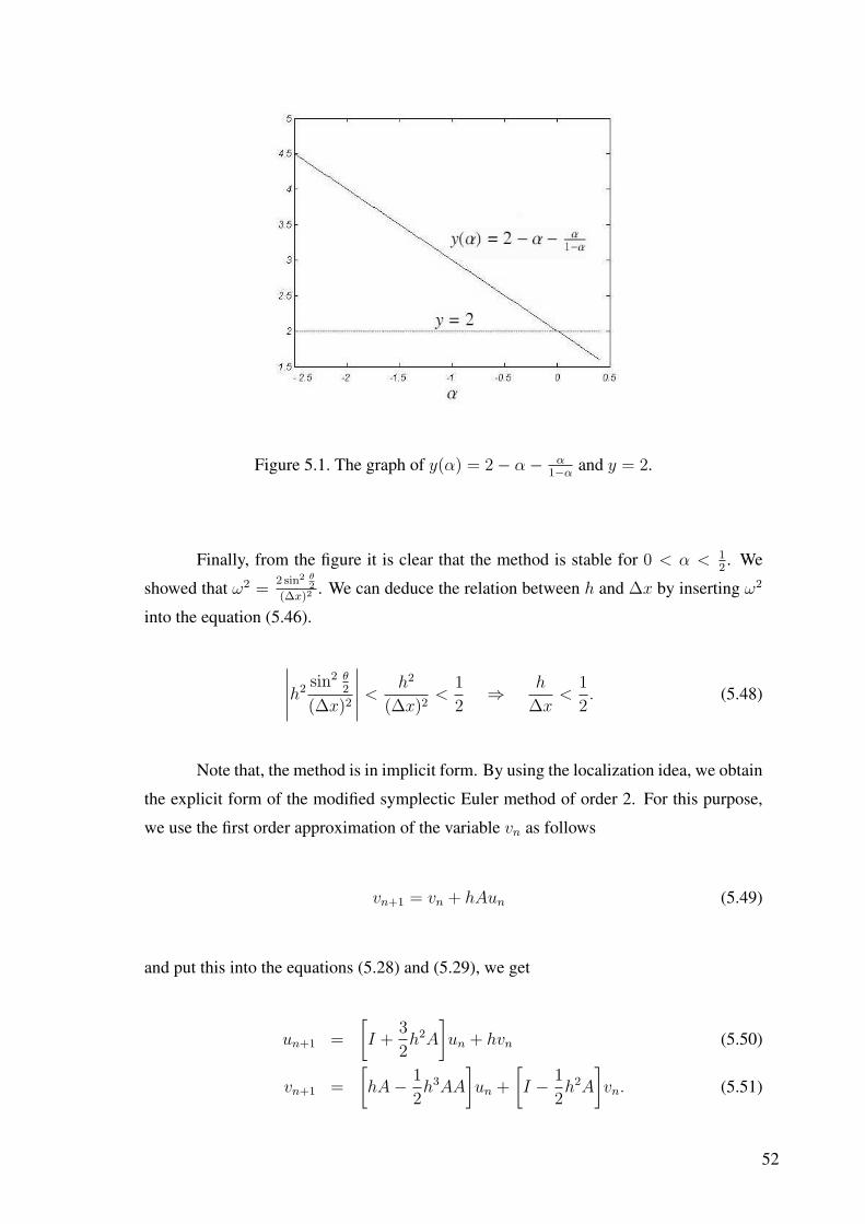
Figure 5.1. The graph of y(α) = 2− α− α1−α

and y = 2.

Finally, from the figure it is clear that the method is stable for 0 < α < 12. We

showed that ω2 =2 sin2 θ

2

(∆x)2. We can deduce the relation between h and ∆x by inserting ω2

into the equation (5.46).

∣∣∣∣∣h2 sin2 θ

2

(∆x)2

∣∣∣∣∣ <h2

(∆x)2<

1

2⇒ h

∆x<

1

2. (5.48)

Note that, the method is in implicit form. By using the localization idea, we obtain

the explicit form of the modified symplectic Euler method of order 2. For this purpose,

we use the first order approximation of the variable vn as follows

vn+1 = vn + hAun (5.49)

and put this into the equations (5.28) and (5.29), we get

un+1 =

[I +

3

2h2A

]un + hvn (5.50)

vn+1 =

[hA− 1

2h3AA

]un +

[I − 1

2h2A

]vn. (5.51)

52

The equations (5.50) and (5.51) may be put into the matrix equation as below

(un+1

vn+1

)=

(I + 3

2h2A h

hA− 12h3AA I − 1

2h2A

)(un

vn

). (5.52)

We take a fourier transform of (5.52),

(un+1(ω)

vn+1(ω)

)=

(1− 3

2h2ω2 h

−hω2 − 12h3ω4 1 + 1

2h2ω2

)(un(ω)

vn(ω)

)(5.53)

Determinant of the above matrix gives the symplecticity of the explicit form of modified

symplectic Euler method. Trace of the above matrix is |2− h2ω2|. By setting 2α = h2ω2,

we get |2 − 2α| < 2. The method is stable for 0 < α < 12. We can deduce the relation

between h and ∆x by inserting ω2 into the equation (5.46).

∣∣∣∣∣h2 sin2 θ

2

(∆x)2

∣∣∣∣∣ <h2

(∆x)2<

1

2⇒ h

∆x<

1√2. (5.54)

Application of 3rd order modified symplectic Euler method to linear wave equa-

tion yields

un+1 = un + h[vn+1 +h

2Aun − h2

3Avn+1] (5.55)

vn+1 = vn + h[Aun − h

2Avn+1 − h2

3AAun]. (5.56)

The equations (5.55) and (5.56) may be put into the matrix equation as below

(I −hI + h3

3A

0 I + h2

2A

)(un+1

vn+1

)=

(I + h2

2A 0

hA− h3

3AA I

)(un

vn

). (5.57)

53

Taking a fourier transform of (5.57), we have

(un+1(ω)

vn+1(ω)

)=

1− h2

2ω2 − ω2(h+h3

3ω2)2

1−h2

2ω2

h+h3

3ω2

1−h2

2ω2

−ω2 h+h3

3ω2

1−h2

2ω2

1

1−h2

2ω2

︸ ︷︷ ︸C

(un(ω)

vn(ω)

)(5.58)

det(C) = 1 gives the symplecticity. For stability, we require

|Tr(C)| < 2 ⇒∣∣∣∣2− 2h2ω2 − 5

12h4ω4 − 1

9h6ω6

1− 12h2ω2

∣∣∣∣ < 2. (5.59)

with the above inequality.

5.2.2. Sine-Gordon Equation

Sine-Gordon equation can be described as

utt − uxx + sin u = 0 (5.60)

for all (x, t) ∈ R× (0,∞).

Equation (5.60) can be written as an infinite dimensional Hamiltonian system by

letting ut = v and vt = uxx − sin u,

ut = −δH

δv(u, v), vt =

δH

δu(u, v) (5.61)

with Hamiltonian functional

H(u, v) =

∫

R

[1

2(−u2

x − v2) + cos u] dx (5.62)

where sin u is a smooth function of u. The solution (u(x, t), v(x, t)), as a time-t map in

the phase space, is symplectic. The equation (5.62) is discretized using central difference

54

approximation for ux with the Hamiltonian

H(u, v) =1

2

n∑i=1

[− 1

2

(ui+1 − ui−1

2∆x

)2 − 1

2v2

i + cos ui

]. (5.63)

Hamilton’s equations for the Sine-Gordon equation in 1 space dimension are

∂

∂tu(x, t) = v(x, t),

∂

∂tv(x, t) =

∂2

∂x2u(x, t)− sin(u(x, t)). (5.64)

A linearisation about the steady state u = 0 gives the equations

∂

∂tu(x, t) = v(x, t),

∂

∂tv(x, t) =

∂2

∂x2u(x, t)− (u(x, t)) = Au (5.65)

where A = ∂xx − I is a linear operator.

Application of 2nd order modified symplectic Euler method to Sine-Gordon equa-

tion yields the same result with linear wave equation. The only difference between linear

wave equation and Sine-Gordon equation is the linear operator. We have the matrix (5.30)

and take the fourier transform of (5.30) with A = ∂xx − I,

(un+1(ω)

vn+1(ω)

)=

1− h2

2(ω2 + 1)− h2(ω2+1)

1−h2

2(ω2+1)

h

1−h2

2(ω2+1)

− h(ω2+1)

1−h2

2(ω2+1)

1

1−h2

2(ω2+1)

(un(ω)

vn(ω)

)(5.66)

and trace of the matrix satisfies the stability with the following condition

∣∣∣∣2−h2

2(ω2 + 1)−

h2

2(ω2 + 1)

1− h2

2(ω2 + 1)

∣∣∣∣ < 2. (5.67)

Application of 3rd order modified symplectic Euler method to Sine-Gordon equation

yields the same result with linear wave equation. The only difference between (5.22)

and (5.60) is the linear operator. We have the matrix (5.57) and take the fourier transform

55

of (5.57) with A = ∂xx − I,

1− h2

2(ω2 + 1)− (ω2+1)(h+h3

3(ω2+1))2

1−h2

2(ω2+1)

h+h3

3(ω2+1)

1−h2

2(ω2+1)

−(ω2 + 1)h+h3

3(ω2+1)

1−h2

2(ω2+1)

1

1−h2

2(ω2+1)

(5.68)

and trace of the above matrix satisfies the stability

∣∣∣∣2− 2h2(ω2 + 1)− 5

12h4(ω2 + 1)2 − 1

9h6(ω2 + 1)3

1− 12h2(ω2 + 1)

∣∣∣∣ < 2. (5.69)

with the above condition.

5.2.3. Schrodinger Equation

Consider the linear time dependent Scrodinger equation

i∂

∂tψ(x, t) =

(− 1

2µ

∂2

∂t2+ V (x)

)ψ(x, t) (5.70)

with V (x) = D(1− e−αx)2. It is separable in its kinetic and potential parts. The solution

of the discretised equation is given by

id

dtc(t) = Hc(t) ⇒ c(t) = e−itHc(0) (5.71)

Consider c = q + ip then i ddt

(q + ip) = H(q + ip), then the Hamiltonian system is

H =1

2pTHp +

1

2qTHq (5.72)

and we have the separable system of Scrodinger equation

q = Hp and p = −Hq (5.73)

56

with formal solution

O(t) =

(cos(tH) sin(tH)

− sin(tH) cos(tH)

)(5.74)

It is an orthogonal and symplectic operator.

Equation (5.70) can be written as an infinite dimensional Hamiltonian system by

letting ut = (−vxx + V (x))v and vt = (uxx − V (x))u.

The Hamiltonian functional

H(u, v) =1

2

∫

R

[u2x + v2

x + V (x)(u2 + v2)] dx. (5.75)

Hamilton’s equations for the Schrodinger equation are

∂

∂tu(x, t) =

(− ∂2

∂x2+ D(1− e−αx)2

)v(x, t), (5.76)

∂

∂tv(x, t) =

( ∂2

∂x2−D(1− e−αx)2

)u(x, t). (5.77)

Since |V (x)| = |D(1 − e−αx)2| ≤ 1 then V (x) = 1. Hamilton’s equations can be taken

as

∂

∂tu(x, t) =

(− ∂2

∂x2+ 1

)v(x, t),

∂

∂tv(x, t) =

( ∂2

∂x2− 1

)u(x, t). (5.78)

where H = −∂xx + 1 is a linear operator.

q = u =(− ∂2

∂x2+ D(1− e−αx)2

)v = Hv (5.79)

p = v =( ∂2

∂x2−D(1− e−αx)2

)u = −Hu (5.80)

Application of 2nd order modified symplectic Euler method to Schrodinger equation

57

yields

un+1 = un + h[Hvn+1 − h

2H2un] (5.81)

vn+1 = vn + h[−Hun +h

2H2vn+1]. (5.82)

The equations (5.81) and (5.82) may be put into the matrix equation as below

(I −hH

0 I − h2

2H2

)(un+1

vn+1

)=

(I − h2

2H2 0

−hH I

)(un

vn

). (5.83)

Fourier transform of (5.83) gives

(1 −h(ω2 + 1)

0 1− h2

2(ω2 + 1)2

)

︸ ︷︷ ︸B

(un+1(ω)

vn+1(ω)

)=

(1− h2

2(ω2 + 1)2 0

−h(ω2 + 1) 1

)(un(ω)

vn(ω)

)(5.84)

We take the inverse of B,

(un+1(ω)

vn+1(ω)

)=

1− h2

2(ω2 + 1)2 − h2(ω2+1)2

1−h2

2(ω2+1)2

h(ω2+1)

1−h2

2(ω2+1)2

− h(ω2+1)

1−h2

2(ω2+1)2

1

1−h2

2(ω2+1)2

(un(ω)

vn(ω)

)(5.85)

Since determinant of the above matrix is 1, it gives the symplecticity. For stability we

require

∣∣∣∣2−h2

2(ω2 + 1)2 −

h2

2(ω2 + 1)2

1− h2

2(ω2 + 1)2

∣∣∣∣ < 2 (5.86)

Application of 3rd order modified symplectic Euler method to linear wave equation yields

un+1 = un + h[Hvn+1 − h

2H2un +

h2

3H3vn+1] (5.87)

vn+1 = vn + h[−Hun +h

2H2vn+1 − h2

3H3un]. (5.88)

58

The equations (5.87) and (5.88) may be put into the matrix equation as below

(I −hH− h3

3H3

0 I − h2

2H2

)(un+1

vn+1

)=

(I − h2

2H2 0

−hH− h3

3H3 I

)(un

vn

). (5.89)

Taking a fourier transform of (5.89), we have the following matrix

1− h2

2(ω2 + 1)2 − (h(ω2+1)+h3

3(ω2+1)3)2

1−h2

2(ω2+1)2

h(ω2+1)+h3

3(ω2+1)3

1−h2

2(ω2+1)2

−h(ω2+1)+h3

3(ω2+1)3

1−h2

2(ω2+1)2

1

1−h2

2(ω2+1)2

(5.90)

For stability, we require

∣∣∣∣2− 2h2(ω2 + 1)2 − 5

12h4(ω2 + 1)4 − 1

9h6(ω2 + 1)6

1− 12h2(ω2 + 1)2

∣∣∣∣ < 2. (5.91)

59

CHAPTER 6

NUMERICAL EXPERIMENT

In this chapter, we make qualitative comparisons of fixed step symplectic integra-

tors of separable Hamiltonian systems.

6.1. Numerical Results of Hamiltonian ODE Problems

In this section the modified Lobatto IIIA-IIIB pair method of order 4 (ML4) is

applied to both linear and nonlinear Hamiltonian systems. The numerical results are

compared with the classical method. For this purpose, Harmonic oscillation is chosen

as linear test problem and Double Well is chosen as nonlinear test problem in order to

show performance of the proposed method.

6.1.1. Applications to Harmonic Oscillator System

In this section we apply the modified differential equations based on the midpoint

method and Lobatto IIIA-IIIB methods for the linear Hamiltonian system, particularly,

Harmonic Oscillator system. Furthermore, the trajectory of motion (phase space), error

in Hamiltonian and global error in the Hamiltonian |H(q, p)−H(q0, p0)| are illustrated.

The Hamiltonian of this system can be given by

H(q, p) =1

2p2 +

1

2q2 (6.1)

so that the equations of motion become

q = Hp(q, p) = p (6.2)

p = Hq(q, p) = −q (6.3)

60

6.1.2. Modified Equations Based on Lobatto IIIA-IIIB Methods

In this section we apply the modified differential equations of the system

q = p = f(p) (6.4)

p = −q = −Vq(q) = g(q) (6.5)

based on Lobatto IIIA-IIIB methods. Applying (6.4) and (6.5) to the modified equations

q′ = p +h2

6gqp =

(I − h2

6Vqq

)p

p′ = −Vq(q)− h2

12(gqq(p, p) + gqg).

(6.6)

we obtain the modified differential equations of the system (6.4) and (6.5) in the following

form

q′ =

(1− h2

6

)p (6.7)

p′ = −q

(1 +

h2

12

). (6.8)

and we apply the methods in the following section.

6.1.3. Numerical Implementation for Harmonic Oscillation

In this section numerical methods are applied to the Harmonic oscillator system.

We apply Lobatto IIIA-IIIB pair of order 2, Lobatto IIIA-IIIB pair of order 4, Runge Kutta

method (order 4), modified Midpoint method (order 4), Gauss collocation method (order

4) to the system (6.4) and (6.5) and modified Lobatto method of order 4 to the system

(6.7) and (6.8). We compare the methods for (p0, q0) = (1, 0) with the step h = 10−2 on

the interval [0, 1].

The Figures (6.1-6.6) illustrate errors in Hamiltonian and global errors in Hamil-

61

tonian (conservation of energy) obtained by Lobatto IIIA-IIIB pair of order 2, Lobatto

IIIA-IIIB pair of order 4, Runge Kutta method (order 4), modified Midpoint method (or-

der 4), Gauss collocation method (order 4) and proposed method (ML4) respectively.

Since all of these methods are symplectic geometric integrators the shape of the trajectory

preserved by these methods. Modified Lobatto method conserves the energy better than

the other methods except Gauss collocation method.

0 2000 4000 6000 8000 10000 120000

0.5

1

1.5x 10

−5 Energy Error

Time t

|H(q

,p)−

H(q

0,p0

)|

0 2000 4000 6000 8000 10000 120000

2

4

6x 10

−4 Global Error

Time t

Figure 6.1. Error in Hamiltonian and global error in Hamiltonian by Lobatto IIIA-IIIBmethod of order 2.

62

0 2000 4000 6000 8000 10000 120000

2

4

6x 10

−6 Energy Error

Time t|H

(q,p

)−H

(q0,

p0)|

0 2000 4000 6000 8000 10000 120000

2

4

6x 10

−4 Global Error

Time t

Figure 6.2. Error in Hamiltonian and global error in Hamiltonian by Lobatto IIIA-IIIBmethod of order 4.

0 2000 4000 6000 8000 10000 120000

2

4

6

8x 10

−11 Energy Error

Time t

|H(q

,p)−

H(q

0,p0

)|

0 2000 4000 6000 8000 10000 120000

0.2

0.4

0.6

0.8

1x 10

−8 Global Error

Time t

Figure 6.3. Error in Hamiltonian and global error in Hamiltonian by Runge Kuttamethod of order 4.

63

0 2000 4000 6000 8000 10000 120000

2

4

6

8x 10

−13 Energy Error

Time t|H

(q,p

)−H

(q0,

p0)|

0 2000 4000 6000 8000 10000 120000

0.2

0.4

0.6

0.8

1x 10

−8 Global Error

Time t

Figure 6.4. Error in Hamiltonian and global error in Hamiltonian by modified Mid-point method of order 4.

0 2000 4000 6000 8000 10000 120000

1

2

3

4x 10

−15 Energy Error

Time t

|H(q

,p)−

H(q

0,p0

)|

0 2000 4000 6000 8000 10000 120000

0.002

0.004

0.006

0.008

0.01Global Error

Time t

Figure 6.5. Error in Hamiltonian and global error in Hamiltonian by Gauss collocationmethod of order 4.

64

0 2000 4000 6000 8000 10000 120000

2

4

6x 10

−15 Energy Error

Time t

|H(q

,p)−

H(q

0,p0

)|

0 2000 4000 6000 8000 10000 120000

0.2

0.4

0.6

0.8

1x 10

−8 Global Error

Time t

Figure 6.6. Error in Hamiltonian and global error in Hamiltonian by the proposedmethod (ML4).

6.1.3.1. Comparison of the Norm of Global Error, Norm of Error in

Hamiltonian and CPU Time

In this section norm of global error, norm of error in Hamiltonian and CPU time

are verified.

The Tables (6.1-6.3) illustrate the norm of global error, norm of error in Hamil-

tonian and CPU time (seconds) in Hamiltonian (conservation of energy) obtained by Lo-

batto IIIA-IIIB pair of order 2, Lobatto IIIA-IIIB pair of order 4, Runge Kutta method

(order 4), modified Midpoint method (order 4), Gauss collocation method (order 4) and

modified Lobatto method of order 4 respectively.

Norm of global errorLobatto method of order 2 0.0169Lobatto method of order 4 0.0225

Runge Kutta method of order 4 3.4242e-007Modified Midpoint of order 4 3.4245e-007

Gauss Collocation method of order 4 0.7056Modified Lobatto method of order 4 3.3803e-007

Table 6.1. Comparison of the norm of global errors in Hamiltonian.

65

Norm of error in HamiltonianLobatto method of order 2 7.6744e-004Lobatto method of order 4 2.5342e-004

Runge Kutta method of order 4 4.0099e-009Modified Midpoint of order 4 2.2983e-011

Gauss Collocation method of order 4 1.6687e-013Modified Lobatto method of order 4 1.6428e-013

Table 6.2. Comparison of the norm of errors in Hamiltonian.

CPU time (seconds)Lobatto method of order 2 0.874Lobatto method of order 4 1.085

Runge Kutta method of order 4 0.577Modified Midpoint of order 4 0.733

Gauss Collocation method of order 4 2.366Modified Lobatto method of order 4 0.589

Table 6.3. Comparison of CPU times (seconds) in Hamiltonian.

The comparison of these six methods reveal that the proposed method (ML4) gives

better performance with respect to the norm of global error, norm of error in Hamiltonian

and CPU time.

6.2. Applications to Double Well System

In this section we determine the modified differential equations based on the Lo-

batto IIIA-IIIB, Gauss collocation methods for the nonlinear Hamiltonian system which

is called Double Well system and illustrate the trajectory of motion (phase space) and the

errors in Hamiltonian |H(q, p)−H(q0, p0)|. The Hamiltonian of this system can be given

by

H(q, p) =1

2p2 +

1

2(q2 − 1)2, (6.9)

66

so that the equations of motion become

q = Hp(q, p) = p (6.10)

p = Hq(q, p) = −2q(q2 − 1) (6.11)

We derive only the modified differential equations of the system (6.10) and (6.11) based

on Lobatto IIIA-IIIB methods. Applying (6.10) and (6.11) to the modified equations

q′ = p +h2

6gqp =

(I − h2

6Vqq

)p

p′ = −Vq(q)− h2

12(gqq(p, p) + gqg).

(6.12)

we obtain the modified differential equations of the system (6.10) and (6.11) in the form

q′ =

[1 +

h2

6

(− 6q2 + 2)]

p (6.13)

p′ = −2q3 + 2q + h2

(qp2 − q5 +

4

3q3 − q

3

). (6.14)

then we apply the methods in the below section.

6.2.1. Numerical Implementation for Double Well

In this part of thesis, numerical methods are applied to the Double Well system.

We apply Gauss collocation method (order 4), Lobatto IIIA-IIIB pair of order 2, ODE

45 to the system (6.10) and (6.11), Lobatto IIIA-IIIB pair of order 4 to the system (6.13)

and (6.14). We compare the methods for (p0, q0) = (1, 0) with the step h = 10−2 on the

interval [0, 1].

The Figures (6.7-6.10) illustrate the trajectory of motion and errors in Hamiltonian

(conservation of energy) obtained by Gauss collocation method (order 4), Lobatto IIIA-

IIIB pair of order 2, Lobatto IIIA-IIIB pair of order 4 and ODE 45 respectively. Since all

of these methods are symplectic the shape of the trajectory preserved by these methods.

ML4 method conserves the energy better than ODE 45 except Gauss collocation method.

67

−2 −1.5 −1 −0.5 0 0.5 1 1.5 2−1.5

−1

−0.5

0

0.5

1

1.5Phase Plane

q

p

0 2000 4000 6000 8000 10000 120000

0.5

1

1.5

2x 10

−9 Energy Error

Time t

|H(q

,p)−

H(q

0,p0

)|

Figure 6.7. Trajectory of motion and error in Hamiltonian by 4th order Gauss colloca-tion method.

−2 −1.5 −1 −0.5 0 0.5 1 1.5 2−1.5

−1

−0.5

0

0.5

1

1.5Phase Plane

q

p

0 2000 4000 6000 8000 10000 120000

0.2

0.4

0.6

0.8

1

1.2x 10

−4 Energy Error

Time t

|H(q

,p)−

H(q

0,p0

)|

Figure 6.8. Trajectory of motion and error in Hamiltonian by 2nd order Lobatto IIIA-IIIB method.

68

−2 −1.5 −1 −0.5 0 0.5 1 1.5 2−1.5

−1

−0.5

0

0.5

1

1.5Phase Plane

q

p

0 2000 4000 6000 8000 10000 120000

1

2

3

4

5

6

7x 10

−5 Energy Error

Time t

|H(q

,p)−

H(q

0,p0

)|

Figure 6.9. Trajectory of motion and error in Hamiltonian by 4th order modified Lo-batto method.

−2 −1.5 −1 −0.5 0 0.5 1 1.5 2−1.5

−1

−0.5

0

0.5

1

1.5Phase Plane

q

p

0 2000 4000 6000 8000 10000 120000

0.1

0.2

0.3

0.4

0.5

0.6

0.7Energy Error

Time t

|H(q

,p)−

H(q

0,p0

)|

Figure 6.10. Trajectory of motion and error in Hamiltonian by ODE45.

69

The comparison of the four method reveals that proposed method conserves the

energy better than ODE 45 except Gauss collocation method.

6.3. Numerical Results of Hamiltonian PDE Problems

In this section, modified symplectic Euler method is applied to PDE problems.

Linear wave equation and Sine-Gordon equation are chosen as test problems.

6.3.1. Linear Wave Equation

Hamiltonian’s equation for the 1-dimensional linear wave equation

utt − uxx = 0 (6.15)

in separable form,

∂u(x, t)

∂t= v(x, t) (6.16)

∂v(x, t)

∂t=

∂2u(x, t)

∂x2= Au = F(u) (6.17)

with the initial conditions

u(x, 0) = sin πx, ut(x, 0) = 0 (6.18)

and boundary conditions

u(0, t) = 0, u(1, t) = 0, (6.19)

70

at x = 0 and x = 1.

We apply modified symplectic Euler method of order 2 to (6.16) and (6.17),

un+1 = un + hvn+1 +h2

2Aun (6.20)

vn+1 = vn + hAun − h2

2

[∂F(u)

∂uvn+1

](6.21)

where h is step size.

We apply central difference method to (6.17) and the linear wave equations given

in (6.16), (6.17) get this form,

ui = vi and vi =ui+1 − 2ui + ui−1

(∆x)2= Au (6.22)

where A is a tridiagonal square matrix of the form

−2 1 0 0 · · · 0

1 −2 1 0 · · · 0

0 1 −2 1 · · · 0... . . . . . . . . . · · · ...

0 0 0 1 −2 1

0 0 · · · 0 1 −2

, (6.23)

i = 1, . . . , n and ∆x is mesh size.

Modified symplectic Euler method of order 2 for the separable system (6.22) can

be written in implicit form as

un+1i = un

i + hvn+1i +

h2

2

[un

i+1 − 2uni + un

i−1

(∆x)2

](6.24)

vn+1i = vn

i + h

[un

i+1 − 2uni + un

i−1

(∆x)2

]− h2

2

[vn+1

i+1 − 2vn+1i + vn+1

i−1

(∆x)2

](6.25)

71

and explicit form as

un+1i = un

i + hvni +

3

2h2

[un

i+1 − 2uni + un

i−1

(∆x)2

](6.26)

vn+1i = h

uni+1 − 2un

i + uni−1

(∆x)2− 1

2h3

[un

i+1 − 2uni + un

i−1

(∆x)2

]2

+vni −

h2

2

vni+1 − 2vn

i + vni−1

(∆x)2(6.27)

where u = (u0, u1, . . . , un)T ,v = (v0, v1, . . . , vn)T are n + 1 dimensional vectors, A is a

tridiagonal n + 1× n + 1 dimensional matrix, h is step size and ∆x is mesh size.

Now we can apply modified symplectic Euler method with given above equations

on the space interval [0, 1] with boundary conditions u(0, t) = 0, u(1, t) = 0, at x = 0

and x = 1 using the following parameters set:

Space interval x = [0, 1]

Space discretization step ∆x = 0.01/0.02/0.04

Time discretization step ∆t = 0.001

Amount of time steps T = 1000

We start with comparison of errors in linear wave problem after applying explicit and

implicit form of modified symplectic Euler method with space discretization step ∆x =

0.01, 0.02 and 0.04 and time discretization step ∆t = 0.001 respectively.

The comparison of errors measured by L∞ and L1 are given in Table 6.4. The

errors used in our computations are calculated by the following equations,

errL∞ := max(max(|u(xi, tn − uanaly(xi, t

n)|)) (6.28)

errL1 :=m∑

i=1

∆x|u(xi, tn − uanaly(xi, t

n)| (6.29)

with respect to given parameters.

72

Nx=100, Nt=1000 errL∞ errL1

SE 0.5001 0.2509SV2 0.0392 0.0192

MSE2-IMP 0.0388 0.0192MSE2-EXP 0.0315 0.0184

Nx=50, Nt=1000 errL∞ errL1

SE 0.5149 0.2535SV2 0.0756 0.0372

MSE2-IMP 0.0744 0.0371MSE2-EXP 0.0660 0.0355

Nx=25, Nt=1000 errL∞ errL1

SE 0.5310 0.2554SV2 0.1522 0.0695

MSE2-IMP 0.1519 0.0695MSE2-EXP 0.1383 0.0645

Table 6.4. Comparison of errors in linear wave problem measured by L∞ norm and L1

norm after applying symplectic Euler method (SE), Stormer Verlet methodof order 2 (SV2), modified symplectic method of order 2 (MSE2) in im-plicit and explicit form respectively.

From the Table 6.4 we conclude that the number of space discretization point

decreases, the accuracy of the solution obtained by the new proposed method increases.

In other words, when the size of the matrix to be solved decreases, the accuracy of the

solution obtained by the proposed increases. The accuracy of the solution obtained by

the proposed and Stormer Verlet method are nearly equal. On the other hand, the explicit

form of modified symplectic Euler method is more accurant for the small system than the

methods we compared with.

6.3.2. Sine-Gordon Equation

Consider an IVP for the Sine-Gordon equation:

utt − uxx + sin(u) = 0 (6.30)

73

on the interval x ∈ [a, b] with initial conditions

u(x, 0) = f(x), ut(x, 0) = g(x), (6.31)

and with, e.g., no-flux boundary conditions

∂u

∂x

∣∣∣∣x=a,b

= 0. (6.32)

Hamiltonian’s equations for Sine-Gordon equation are

∂u(x, t)

∂t= v(x, t) (6.33)

∂v(x, t)

∂t=

∂2u(x, t)

∂x2− sin(u(x, t)) = Au− sin u = F(u). (6.34)

We apply modified symplectic Euler method of order 2 to (6.33) and (6.34),

un+1 = un + hvn+1 +h2

2F(un) (6.35)

vn+1 = vn + hF(un)− h2

2

[∂F

∂uvn+1

]. (6.36)

We apply central difference method to (6.34) and Sine-Gordon equations get this form,

ui = vi and vi =ui+1 − 2ui + ui−1

(∆x)2− sin ui = Au− β (6.37)

74

where A is a tridiagonal n + 1× n + 1 square matrix of the form

−2 1 0 0 · · · 0

1 −2 1 0 · · · 0

0 1 −2 1 · · · 0... . . . . . . . . . · · · ...

0 0 0 1 −2 1

0 0 · · · 0 1 −2

, (6.38)

β = (sin(u0), sin(u1), . . . , sin(un))T is a n + 1-dimensional vector, and ∆x is mesh size.

Modified symplectic Euler method of order 2 for the separable system (6.37) can

be written as

un+1i = un

i + hvn+1i +

h2

2

[un

i+1 − 2uni + un

i−1

(∆x)2− sin(un

i )

](6.39)

vn+1i = vn

i + h

[un

i+1 − 2uni + un

i−1

(∆x)2− sin(un

i )

]

−h2

2

[vn+1

i+1 − 2vn+1i + vn+1

i−1

(∆x)2− vn+1

i cos(uni )

](6.40)

where h is step size and ∆x is mesh size.

Now we can apply the given schemes (6.39) and (6.40) described above to eq.

(6.31). Let us solve it on the interval [−L,L] with no-flux boundary conditions using the

following parameters set:

Space interval L = 20

Space discretization step ∆x = 0.1

Time discretization step ∆t = 0.05

Velocity of the kink c = 0.2

We use the different initial conditions for Sine-Gordon equation to simulate by using

modified symplectic Euler method of order 2 and start with the numerical representation

75

of kink and antikink solutions. The initial condition for the kink soliton is

f(x) = 4 arctan

(exp

(x√

1− c2

)), (6.41)

g(x) = −2c√

1− c2sec h

(x√

1− c2

). (6.42)

Figure (6.11) shows the space-time plot of the numerical kink solution.

−20 −15 −10 −5 0 5 10 15 20−1

0

1

2

3

4

5

6

7

x

u(x,

t)

−20−10

010

20

0

0.5

1−2

0

2

4

6

8

xt

u(x,

t)

Figure 6.11. Numerical solution of (6.31), calculated with given schemes for the case ofthe kink solitons, moving with the velocity c = 0.2. Space-time informationis shown.

For the antikink soliton, the initial condition reads

f(x) = 4 arctan

(exp

(− x√

1− c2

)), (6.43)

g(x) = −2c√

1− c2sec h

(x√

1− c2

). (6.44)

Numerical solutions is shown on Figure (6.12).

76

−20 −15 −10 −5 0 5 10 15 20−1

0

1

2

3

4

5

6

7

x

u(x,

t)

−20−10

010

200

0.20.4

0.60.8

1

−2

0

2

4

6

8

tx

u(x,

t)

Figure 6.12. Numerical solution of (6.31), calculated with given schemes for the caseof the antikink solitons, moving with the velocity c = 0.2. Space-timeinformation is shown.

Now we are in position to find numerical solutions, corresponding to kink-kink

and kink-antikink collisions. For the kink-kink collision we choose

f(x) = 4 arctan

(exp

(x + L/2√

1− c2

))+ 4 arctan

(exp

(x− L/2√

1− c2

)), (6.45)

g(x) = −2c√

1− c2sec h

(x + L/2√

1− c2

)+ 2

c√1− c2

sec h

(x− L/2√

1− c2

), (6.46)

whereas for the kink-antikink collision the initial conditions are

f(x) = 4 arctan

(exp

(x + L/2√

1− c2

))+ 4 arctan

(exp

(− x− L/2√

1− c2

)),(6.47)

g(x) = −2c√

1− c2sec h

(x + L/2√

1− c2

)− 2

c√1− c2

sec h

(x− L/2√

1− c2

). (6.48)

Numerical solutions, corresponding to both cases is presented on Figure (6.13) and (6.14),

respectively.

77

−20 −15 −10 −5 0 5 10 15 200

2

4

6

8

10

12

14

x

u(x,

t)

−20

−10

0

10

20

00.20.40.60.81

0

5

10

15

x

t

u(x,

t)Figure 6.13. Space-time representation of the numerical solution of (6.31) for kink-kink

collision.

−20 −15 −10 −5 0 5 10 15 206

7

8

9

10

11

12

13

x

u(x,

t)

−20−10

010

20

0

0.5

1

6

8

10

12

14

xt

u(x,

t)

Figure 6.14. Space-time representation of the numerical solution of (6.31) for kink-antikink collision.

78

Finally, for the case of breather solution we choose

f(x) = 0, (6.49)

g(x) = 4√

1− c2 sec h(x√

1− c2). (6.50)

Corresponding numerical solution is presented on Figure (6.15).

−20 −15 −10 −5 0 5 10 15 200

0.5

1

1.5

2

2.5

3

3.5

x

u(x,

t)

−20

0

200 0.2 0.4 0.6 0.8 1

0

0.5

1

1.5

2

2.5

3

3.5

x

t

u(x,

t)

Figure 6.15. Space-time representation of the numerical solution of (6.31) for breathersolution.

Modified symplectic Euler method is applied to Sine-Gordon equation with soliton so-

lutions for various combinations of parameters under no-flux boundary conditions. We

have different simulations for various combinations of parameters.

79

CHAPTER 7

CONCLUSION

Throughout this thesis we have used an approach that was developed by using

the idea in backward error analysis while constructing modified equations by inverting

the roles of the exact and numerical flows. In this case, we have constructed 4th order

modified Lobatto IIIA-IIIB pair method (ML4) by using modified vector field idea.

After presenting this new method, its convergence properties are analyzed using

concepts familiar from numerical analysis of stability, consistency and order.

In the next chapter, the modified symplectic Euler method of order 2 and 3 that

were constructed by using the modified vector field idea are applied to linear and non-

linear PDE problems. In addition we present the Von-Neumann stability analysis of the

differential equations we considered.

In the numerical experiment section, first harmonic oscillation problem is exam-

ined as a first test problem. In particular error in Hamiltonian, global error and phase

plane are investigated with respect to the six different algorithms for Harmonic oscilla-

tion problem. In our investigation of accuracy and efficiency of these algorithms we found

the followings:

• The shape of the trajectories are preserved by these methods.

• Comparisons of the 4th order methods showed that ML4 method is more efficient

with respect to the errors in Hamiltonian, global errors and computational times.

In addition, the Double Well problem is examined as a second test problem. Similar con-

clusions were drawn for the nonlinear ODE problem using ML4 method. ML4 method

conserves the energy better than ODE45, except Gauss collocation method. The numer-

ical results for this part show that not only linear ODE problem, but also nonlinear ODE

problem can be high quality and efficient schemes for the long time behavior by using

ML4 method.

Next, we make qualitative comparisons of fixed step symplectic integrators of sep-

arable Hamiltonian systems. We consider linear wave equation problem as a test problem,

we presented the errors obtained by symplectic Euler method, Stormer-Verlet method of

order 2, modified symplectic method of order 2 in implicit and explicit form measured by

L∞ and L1. The numerical results indicate that

80

• The number of space discretization point decreases, the accuracy of the solution

obtained by the new proposed method increases.

• The explicit form of modified symplectic Euler method is more accurant for the

small system than the methods we compared with.

Finally, modified symplectic Euler method is applied to Sine-Gordon equation with soli-

ton solutions for various combinations of parameters under no-flux boundary conditions.

We have different simulations for various combinations of parameters.

Our computational results reveal that new proposed modified symplectic Euler

and modified Lobatto method are efficient for whole linear ODE and PDE problems.

Using the modified vector field idea, one can apply these symplectic methods for different

Hamiltonian ODE and PDE systems as a future work.

81

REFERENCES

Hairer E., Lubich C., & Wanner G., 2002: Geometric Numerical Integration.Structure-preserving algorithms for ordinary differential equations. Volume 31 ofSpringer Series in Computational Mathematics.

Chartier P., Hairer E., & Vilmart G., 2006: Modified Equations. ESAIM: Proceedings,16-20.

Ahmed M.O. and Corless R.M., 1997: The method of modified equations in Maple.Electronic Proceedings of the 3rd International IMACS Conference on Applica-tions of Computer Algebra., 1-21.

Kozlov R., 2007: Conservative Discritizations of the Kepler Problem. Journal ofPhysics A: Mathematical and Theoretical., 4529-4539.

Strehmel K. & Weiner R., 1984: Partitioned Adaptive Runge-Kutta Methods and TheirStability. Numer. Math., 283-300.

Marsden J.E. & West M., 2001: Discrete mechanics and variational integrators. ActaNumerica., 357-514.

Budd C.J. & Piggott M.D., 2000: Geometric Integration and Its Applications. In hand-book of Numerical Analysis, Vol XI., 35-139.

Wilkinson J.H, 1963: Rounding Errors In Algebraic Process. New Jersey: Prentice-Hall.

Wilkinson J.H, 1965: The Algebraic Eigenvalue Problem. USA: Oxford UniversityPress.

Wilkinson J.H, 1961: Error Analysis of Direct Methods of Matrix Inversion. Journalof the ACM., 8, 281-330.

Olver P.J, 1993: Applications of Lie groups to differential equations. New York:Springer-Verlag.

Hairer E., 1984: Backward Analysis of Numerical Integrators and Symplectic Meth-ods. Annals of Numerical Mathematics., 1, 107-132.

Hairer E., 2005: Important Aspects of Geometric Numerical Integration. Journal ofScientific Computing., 8, 67-81.

82

Hairer E. and Stoffer D., 1997: Reversible Long-Term Integration with Variable Step-Sizes. SIAM J. Sci. Comput., 18, 257-269.

Hairer E. and Wanner G., 1974: On the butcher group and general multivalue methods.Computing., 13, 1-15.

Lambert J., 1991: Numerical Methods for Ordinary Differential Systems. New York:John Wiley and Sons.

Reich S., 1999: Backward Error Analysis for Numerical Integrators. SIAM J. Numer.Anal., 36, 1549-1570.

Moser J. and Veselov A.P, 1991: Discrete versions of some classical integrable systemsand factorization of matrix polynomials. Comm. Math. Phys., 139, 217-243.

McLachlan R.I., 2007: A new implementation of symplectic Runge-Kutta methods.SIAM Journal on Scientific Computing., 1637-1649.

Budd C.J. & Piggott M.D., 2000: Geometric Integration and Its Applications. In hand-book of Numerical Analysis, Vol XI., 35-139.

James E, Howard ,Holger R., & Dullin, 1998: Linear Stability of natural symplecticmaps. Physics Letters A., 246, 273-283.

Regan, Helen, M. 2000: Von Neumann Stability Analaysis of Symplectic IntegratorsApplied to Hamiltonian PDEs. Vol.20., 60 pp.

Lu X. and Schmid R., 1998: Symplectic Integration of Sine-Gordon Type systems.IMACS 1998.

Fausett L.V., 2008: Applied Numerical Analysis Using MATLAB. Texas A.M.University-Commerce.

Demir D., 2009: Higher Order Symplectic Methods Based on Modified Vector Fields.IYTE, Thesis 2009.

83

APPENDIX A

MATLAB CODES FOR NUMERICAL EXPERIMENTS

HIGHER ORDER SYMPLECTIC METHODS MATLAB CODE FOR

HARMONIC OSCILLATION PROBLEM

%%%%% 2nd order Lobatto for harm. osc. problem %%%%%

clear all;

p4(1)= 1;

q4(1)= 0;

h=.01;

t=0:h:100;

n=100/h+1;

for i=1:n

ye(i)=sin(t(i));

end

tic

for i=1:n

H4(i)=.5*(p4(i).ˆ2+q4(i).ˆ2);

L1s(i)=-q4(i);

Ks(i)=p4(i)+h/2*L1s(i);

L2s(i)=-(q4(i)+h*(Ks(i)));

q4(i+1)=q4(i)+h*(Ks(i));

p4(i+1)=p4(i)+(h/2)*(L1s(i)+L2s(i));

e4(i)=abs(H4(i)-H4(1));

er(i)=abs(ye(i)-q4(i));

end

norm(er)

norm(e4)

toc

subplot(211);plot(e4,’r’);

title(’Energy Error’);

xlabel(’Time t’);ylabel(’|H(q,p)-H(q0,p0)|’);

subplot(212);plot(t,er,’m’);

84

title(’Global Error’);

xlabel(’Time t’);

%%%%% 4th order Lobatto for Harm. Osc. problem %%%%%

clear all;

p2(1)=1;

q2(1)=0;

h=.01;

t=0:h:100;

n=100/h+1;

for i=1:n

ye(i)=sin(t(i)); end

tic

for i=1:n

H2(i)=.5*(p2(i).ˆ2+q2(i).ˆ2);

L1(i)=-q2(i);

L2(i)=(-q2(i)-(h/2)*p2(i)-((h.ˆ2)/12)*L1(i))

/(1+((h.ˆ2)/24));

L3(i)=-q2(i)-(h/6)*(6*p2(i)+h*L1(i)-2*h*L2(i));

K1(i)=p2(i)+(h/6)*(L1(i)-L2(i));

K2(i)=p2(i)+(h/6)*(L1(i)+2*L2(i));

K3(i)=p2(i)+(h/6)*(L1(i)+5*L2(i));

q2(i+1)=q2(i)+(h/6)*(K1(i)+4*K2(i)+K3(i));

p2(i+1)=p2(i)+(h/6)*(L1(i)+4*L2(i)+L3(i));

e2(i)=abs(H2(i)-H2(1));

er2(i)=abs(ye(i)-q2(i));

end

norm(er2)

norm(e2)

toc

subplot(211);plot(e2,’r’);

title(’Energy Error’);

xlabel(’Time t’);ylabel(’|H(q,p)-H(q0,p0)|’);

subplot(212);plot(t,er2,’m’);

title(’Global Error’);

xlabel(’Time t’);

85

%%%%% Runge Kutta method of order 4 for Harm.

Osc. problem %%%%%

clear all;

Y=[1;0];

h=.01;

t=0:h:100;

n=100/h+1;

for i=1:n

ye(i)=cos(t(i));

end

tic

for i=1:n

p(i)=Y(1,1);

q(i)=Y(2,1);

H(i)=.5*(p(i).ˆ2+q(i).ˆ2);

C=[0 1;-1 0];

k1=C*Y;

Y1=Y+(1/3)*h*k1;

k2=C*Y1;

Y2=Y+(-1/3)*h*k1+h*k2;

k3=C*Y2;

Y3=Y+h*k1-h*k2+h*k3;

k4=C*Y3;

Y=Y+(1/8)*h*(k1+3*k2+3*k3+k4);

e(i)=abs(H(i)-H(1));

er(i)=abs(ye(i)-p(i));

end

norm(er)

norm(e)

toc

subplot(211);plot(e,’r’);

title(’Energy Error’);

xlabel(’Time t’);ylabel(’|H(q,p)-H(q0,p0)|’);

subplot(212);plot(t,er,’m’);

title(’Global Error’);

86

xlabel(’Time t’);

%%%%% Modified Midpoint of order 4 for harm. osc.

problem %%%%%

clear all;

p3(1)=1;

q3(1)=0;

h=.01;

t=0:h:100;

n=100/h+1;

K=(1+(hˆ2)/12);

A=((1-((h.ˆ2)*K.ˆ2)/4)/(1+((h.ˆ2)*K.ˆ2)/4));

B=((h*K)/(1+((h.ˆ2)*K.ˆ2)/4));

for i=1:n

ye(i)=cos(t(i));

end

tic

for i=1:n

H3(i)=(p3(i).ˆ2+q3(i).ˆ2);

e3(i)=(abs(H3(i)-H3(1)));

p3(i+1)=A*p3(i)+B*q3(i);

q3(i+1)=A*q3(i)-B*p3(i);

er3(i)=abs(ye(i)-p3(i));

end

norm(er3)

norm(e3)

toc

subplot(211);plot(e3,’r’);

title(’Energy Error’);

xlabel(’Time t’);ylabel(’|H(q,p)-H(q0,p0)|’);

subplot(212);plot(t,er3,’m’);

title(’Global Error’);

xlabel(’Time t’);

clear all;

%%%%% Gauss Collocation Method for Harm. Osc. problem %%%%%

p0= 1;

87

q0= 0;

h=.01;

t=0:h:100;

n=100/h+1;

a11=1/4;

a12=1/4-(sqrt(3)/6);

a21=1/4+(sqrt(3)/6);

a22=1/4;

q=q0;

p=p0;

k12p=feval(’qpd’,q,p,h);

k22p=feval(’qpd’,q,p,h);

H0 = .5*(p.ˆ2 + q.ˆ2);

for i=1:n

ye(i)=sin(t(i));

end

tic

for i=1:n

H=.5*(p.ˆ2+q.ˆ2);

for j=1:5

k11=p+h*(a11*k12p+a12*k22p);

k21=p+h*(a21*k12p+a22*k22p);

k12=feval(’qpd’,q+h*(a11*k11+a12*k21),p,h);

k22=feval(’qpd’,q+h*(a21*k11+a22*k21),p,h);

k12p=k12;

k22p=k22;

end

q1=q+h/2*(k11+k21);

p1=p+h/2*(k12+k22);

Q(:,i) = q1;

P(:,i) = p1;

q= q1;

p= p1;

er(i)=abs(ye(i)-q);

H(i)= .5*(p.ˆ2+q.ˆ2) ;

88

error_H(i)= abs(H(i)-H0) ;

end

norm(er)

norm(error_H)

toc

subplot(211);plot(error_H,’r’);

title(’Energy Error’);

xlabel(’Time t’);ylabel(’|H(q,p)-H(q0,p0)|’);

subplot(212);plot(t,er,’m’);

title(’Global Error’);

xlabel(’Time t’);

%%%%% Modified Lobatto method of order 4 for

Harm. Osc. problem %%%%%

p1(1)= 1;

q1(1)= 0;

h=.01;

t=0:h:100;

n=100/h+1;

for i=1:n

ye(i)=sin(t(i));

end

tic

for i=1:n

H1(i)=.5*(p1(i).ˆ2+q1(i).ˆ2);

L11(i)=-q1(i)*(1+(h.ˆ2)/12);

K(i)=(1-(h.ˆ2)/6)*(p1(i)+(h/2)*L11(i));

L22(i)=-(1+(h.ˆ2)/12)*(q1(i)+h*K(i));

q1(i+1)=q1(i)+h*(K(i));

p1(i+1)=p1(i)+(h/2)*(L11(i)+L22(i));

e1(i)=abs(H1(i)-H1(1));

er1(i)=abs(ye(i)-q1(i));

end

norm(er1)

norm(e1)

toc

89

subplot(211);plot(e1,’r’);

title(’Energy Error’);

xlabel(’Time t’);ylabel(’|H(q,p)-H(q0,p0)|’);

subplot(212);plot(t,er1,’m’);

title(’Global Error’);

xlabel(’Time t’);

HIGHER ORDER SYMPLECTIC METHODS MATLAB

CODE FOR DOUBLE WELL PROBLEM

%%%%% Gauss Collocation Method for Double Well %%%%%

clear all;

p0= 1;

q0= 0;

h=.01;

t=0:h:100;

n=100/h+1;

a11=1/4;

a12=1/4-(sqrt(3)/6);

a21=1/4+(sqrt(3)/6);

a22=1/4;

q=q0;

p=p0;

k12p=feval(’qpdd’,q,p,h);

k22p=feval(’qpdd’,q,p,h);

H0 = .5*(p.ˆ2 + (q.ˆ2-1).ˆ2);

tic

for i=1:n

for j=1:10

k11=p+h*(a11*k12p+a12*k22p);

k21=p+h*(a21*k12p+a22*k22p);

k12=feval(’qpdd’,q+h*(a11*k11+a12*k21),p,h);

k22=feval(’qpdd’,q+h*(a21*k11+a22*k21),p,h);

k12p=k12;

k22p=k22;

end

90

q1=q+h/2*(k11+k21);

p1=p+h/2*(k12+k22);

Q(:,i) = q1;

P(:,i) = p1;

q= q1;

p= p1;

H(i)= .5*(p.ˆ2+(q.ˆ2-1).ˆ2) ;

error_H(i)= abs(H(i)-H0) ;

end

toc

subplot(111);plot(error_H,’r’);

title(’Energy Error’);

xlabel(’Time t’);ylabel(’|H(q,p)-H(q0,p0)|’);

%%%%% 2nd order Lobatto method for Double Well %%%%%

clear all;

p0= 1;

q0= 0;

h=.01;

t=0:h:100;

n=100/h+1;

q=q0;

p=p0;

H0 = .5*(p.ˆ2 + (q.ˆ2-1).ˆ2);

L1p=feval(’ppm’,q,p,h);

tic

for i=1:n

% calculation of L1 implicitly

for j=1:5

L1=feval(’ppm’,q, p+h/2*L1p,h);

L1p=L1;

end

k2p=feval(’qpm’,q,p+(h/2)*L1,h);

k1=feval(’qpm’,q,p+h/2*L1,h);

% calculation of k2 implicitly

for j=1:5

91

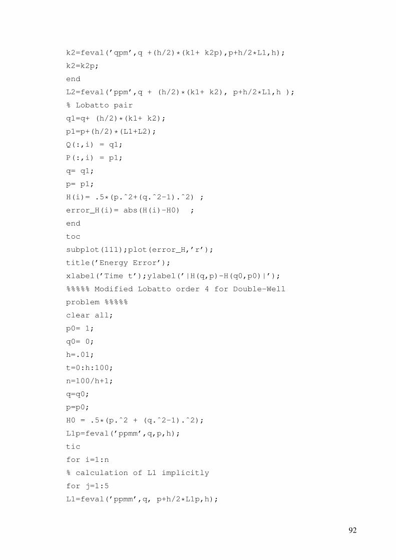
k2=feval(’qpm’,q +(h/2)*(k1+ k2p),p+h/2*L1,h);

k2=k2p;

end

L2=feval(’ppm’,q + (h/2)*(k1+ k2), p+h/2*L1,h );

% Lobatto pair

q1=q+ (h/2)*(k1+ k2);

p1=p+(h/2)*(L1+L2);

Q(:,i) = q1;

P(:,i) = p1;

q= q1;

p= p1;

H(i)= .5*(p.ˆ2+(q.ˆ2-1).ˆ2) ;

error_H(i)= abs(H(i)-H0) ;

end

toc

subplot(111);plot(error_H,’r’);

title(’Energy Error’);

xlabel(’Time t’);ylabel(’|H(q,p)-H(q0,p0)|’);

%%%%% Modified Lobatto order 4 for Double-Well

problem %%%%%

clear all;

p0= 1;

q0= 0;

h=.01;

t=0:h:100;

n=100/h+1;

q=q0;

p=p0;

H0 = .5*(p.ˆ2 + (q.ˆ2-1).ˆ2);

L1p=feval(’ppmm’,q,p,h);

tic

for i=1:n

% calculation of L1 implicitly

for j=1:5

L1=feval(’ppmm’,q, p+h/2*L1p,h);

92

L1p=L1;

end

k2p=feval(’qpmm’,q,p+(h/2)*L1,h);

k1=feval(’qpmm’,q,p+h/2*L1,h);

% calculation of k2 implicitly

for j=1:5

k2=feval(’qpmm’,q +(h/2)*(k1+ k2p),p+h/2*L1,h);

k2=k2p;

end

L2=feval(’ppmm’,q + (h/2)*(k1+ k2), p+h/2*L1,h );

% Lobatto pair

q1=q+ (h/2)*(k1+ k2);

p1=p+(h/2)*(L1+L2);

Q(:,i) = q1;

P(:,i) = p1;

q= q1;

p= p1;

H(i)= .5*(p.ˆ2+(q.ˆ2-1).ˆ2) ;

error_H(i)= abs(H(i)-H0) ;

end

toc

subplot(111);plot(error_H,’r’);

title(’Energy Error’);

xlabel(’Time t’);ylabel(’|H(q,p)-H(q0,p0)|’);

%%%%% ODE 45 for Double-Well problem %%%%%

options = odeset(’RelTol’,1e-4,’AbsTol’,[1e-4 1e-4]);

[t,Y] = ode45(@rigid,[0 870],[-1 1.000001 ],options);

% plot(t,Y(:,1),’-’,t,Y(:,2),’-.’);

q0=-1;

p0=1.000001;

q=Y(:,1);

p=Y(:,2);

n=size(p)

H0= 0.5* (p0.ˆ2) - 0.5* (q0.ˆ2- 1).ˆ2;

tic

93

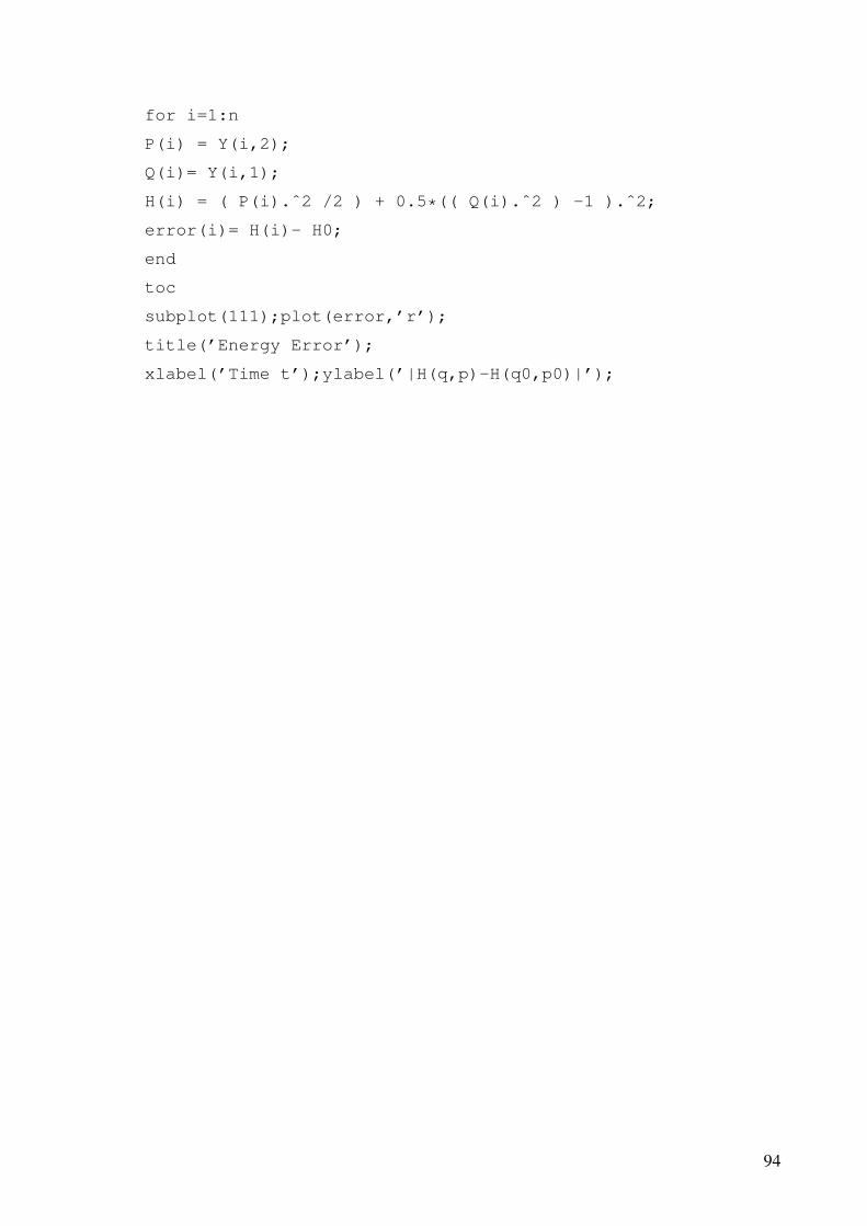
for i=1:n

P(i) = Y(i,2);

Q(i)= Y(i,1);

H(i) = ( P(i).ˆ2 /2 ) + 0.5*(( Q(i).ˆ2 ) -1 ).ˆ2;

error(i)= H(i)- H0;

end

toc

subplot(111);plot(error,’r’);

title(’Energy Error’);

xlabel(’Time t’);ylabel(’|H(q,p)-H(q0,p0)|’);

94