second order conformal symplectic schemes for … · second order conformal symplectic schemes for...

Noname manuscript No.(will be inserted by the editor)

Second Order Conformal Symplectic Schemes forDamped Hamiltonian Systems

Ashish Bhatt · Dwayne Floyd · Brian E. Moore

Received: date / Accepted: date

Abstract Numerical methods for solving weakly damped Hamiltonian sys-tems are constructed using the popular Stormer-Verlet and implicit midpointmethods. Each method is shown to preserve dissipation of symplecticity anddissipation of angular momentum of an N -body system with pairwise dis-tance dependent interactions. Necessary and sufficient conditions for secondorder accuracy are derived. Analysis for linear equations gives explicit rela-tionships between the damping parameter and the step size to reveal whenthe methods are most advantageous; essentially, the damping rate of the nu-merical solution is exactly preserved under these conditions. The methods areapplied to several model problems, both ODEs and PDEs. Additional struc-ture preservation is discovered for the discretized PDEs, in one case dissipationin total linear momentum and in another dissipation in mass are preserved bythe methods. The numerical results, along with comparisons to a higher ordermethod and another structure-preserving method, demonstrate the usefulnessand strengths of the methods.

Keywords conformal symplectic · Rayleigh damping · Birkhoffian method ·structure-preserving algorithm · dissipation preservation

A. BhattDepartment of Mathematics, University of Central Florida, Orlando, Florida, USAE-mail: [email protected]

D. FloydDepartment of Mathematics, University of Central Florida, Orlando, Florida, USAE-mail: floyd dwayne [email protected]

B.E. MooreDepartment of Mathematics, University of Central Florida, Orlando, Florida, USAE-mail: [email protected]

2 A. Bhatt, D. Floyd, B.E. Moore

1 Introduction

Consider a conformal Hamiltonian system [9] with separable HamiltonianH(q, p) = T (p) + V (q)

qt = ∇pT (p), pt = −∇qV (q)− 2γp

where q, p ∈ Rd and γ > 0. In matrix-vector form, with z = [q, p]T , theequation can be stated

Jzt = ∇zH(z) + Dz, (1)

with

z =

[qp

], J =

[0 −II 0

], D =

[0 2γI0 0

],

where I is the d×d identity matrix. By defining Hγ(z) = T (p) +V (q) + γqT p,the equation can also be stated

Jzt = ∇zHγ(z)− γJz, (2)

Dynamical systems of the form (2) arise in many applications, especially formodels of Newtonian mechanics that include frictional forces. Thus, numericalmethods for solving these systems are important, and it is well known that theperformance of numerical schemes commonly used for Hamiltonian systems isnegatively impacted by including a damping term. Nevertheless, numericalsimulations that correctly approximate losses in energy, momentum, phasespace area, etc., are important.

In fact, there have been multiple studies on structure-preserving numericalintegrators for systems with weak dissipation. Variational methods have beenapplied to weakly dissipative systems showing excellent numerical rates ofenergy dissipation compared to other methods [6]. Energy-momentum schemeshave been shown to preserve the relative equilibria [1,2]. There are also finitedifference schemes that preserve dissipative properties of PDEs [5,8].

Prior work most related to the present study includes the use of splittingmethods to exactly preserve the conformal symplectic structure of the sys-tem [10,11]; we use this technique for constructing methods. Other work thatapplies this approach includes methods based on the Stormer-Verlet scheme,which are analyzed using backward error analysis to show that the rate of en-ergy dissipation is asymptotically correct up to an exponentially small error,and the relative equilibria are nearly conserved [13]. Those results depend upondamping coefficients and step-sizes that are sufficiently small. From a practicalstandpoint, we prove that methods of this type preserve several properties ofthe governing equations, and we derive necessary conditions for linear stabil-ity, giving a first look at how small damping coefficients and step-sizes arerequired to be.

Other work that is closely related to the present study is focused on al-gorithms that preserve the structure of Birkhoffian systems, with special em-phasis on implicit midpoint type methods and a damped harmonic oscillator

Second Order Conformal Symplectic Schemes 3

[7,17]. Results of these works show how methods that preserve the symplecticstructure of Birkhoffian systems can be constructed. Backward error analysiswas also performed to show the modified equations are Brikhoffian and there-by possess the same qualitative properties, such as symplecticity. We considera similar implicit midpoint type method, but prove that it is uncondition-ally stable for linear equations and derive conditions that are required for themethod to be second order. We also show that the method exactly preservesproperties of the governing equations, other than the symplectic property.

To be precise about properties of the governing equations that are preservedby the methods we consider, observe the variational equation associated with(2),

Jdzt = ∂zzHγ(z)dz − γJdz.

Taking the wedge product with dz, and using the symmetry of the HessianMatrix ∂zzHγ(z), gives

dz ∧ Jdzt = −γdz ∧ Jdz, =⇒ ∂t(dz ∧ Jdz) = −2γ(dz ∧ Jdz),

i.e. symplectic two form dz ∧ Jdz decays exponentially along the solution ofODE (2). This leads us to introduce the following Definition which is adaptedfrom [9] to our purpose.

Definition 1 A differential equation zt = g(z) is called conformal symplecticif the relation

∂tω = −2γω or equivalently ω(t) = e−2γtω(0)

is satisfied for ω = dz ∧ Jdz and γ ∈ R.

A numerical method zi+1 = ψ∆t(zi) for (1) or (2) is said to preserve conformal

symplecticity, or more simply we call the method conformal symplectic, if itsatisfies

ωi+1 = e−2γ∆tωi

for ωi = ω(zi) = dzi ∧ Jdzi and ∆t = ti+1 − ti.A function P (e.g. energy, momentum, 2-norm of the solution, mass etc.)

of the solution of a differential equation that satisfies

∂tP = −2γP or equivalently P (t) = e−2γtP (0) (3)

is called a conformal property of the differential equation. Since it is desirableto preserve as much of the exact solution behavior as possible, it is desirable forthe numerical method approximating the equation to preserve the conformalproperty P by satisfying

P i+1 = e−2γ∆tP i

for some discrete approximation P i of P (ti). As an example, consider ODE(1) with N-body pairwise distance dependent Hamiltonian

H(q, p) =

N∑n=1

‖pn‖2

2mn+

N−1∑n=1

N∑j=n+1

φnj(‖qn − qj‖) (4)


where mn is mass of the nth particle and φnj(‖qn−qj‖) is interaction potential(pair-potential) between particles n and j at the distance (‖qn−qj‖). Equation(1) gives the following equations of motion for this Hamiltonian

∂tqn =1

mnpn, (5)

∂tpn = −∑j 6=n

τn,j(qn − qj)− 2γpn (6)

for n = 1, 2, . . . , N ; where we define

τn,j =φ′nj(‖qn − qj‖)‖qn − qj‖

.

Taking the cross product of (5) and (6) with pn and qn, respectively, we have

∂tqn × pn = 0,

∂tpn × qn = −∑j 6=n

τn,j(−qj × qn)− 2γpn × qn.

Now, summing the second equation over n gives∑n

∂tpn × qn = −∑n

∑j 6=n

τn,j(−qj × qn)− 2γ∑n

pn × qn

= −2γ∑n

pn × qn,

which implies a special case of (3), given by

∂t

(∑n

pn × qn

)= −2γ

∑n

pn × qn.

Similarly summing equation (6) over n we arrive at∑n

∂tpn = −2γ∑n

pn, ⇐⇒∑n

pn(t) = e−2γt∑n

pn(0).

Therefore, total angular momentum∑n pn(t)× qn(t) and total linear momen-

tum∑n pn(t) are conformal properties for the system of equations (5)-(6).

In addition, to our results on methods for ODEs, we apply the time-stepping schemes to discretize damped Hamiltonian PDEs, showing (analyt-ically and numerically) how the methods are advantageous. Similar relatedwork includes extension of symplectic integrators for Birkhoffian ODEs tomulti-symplectic Birkhoffian PDEs [16], showing how to construct structure-preserving methods through a discrete variational principle, and applying onesuch methods to a damped linear wave equation. Other work, also using amulti-symplectic approach to construct integrators that preserve damping ofsymplecticity of wave equations, in addition to other dissipation properties [14,15], generalizes conformal symplecticity to damped multi-symplectic PDEs in


[14], and an implicit midpoint type discretization was analyzed in [15]. Themethods of both articles are first order time integrators, but we build on thoseresults to present second-order structure-preserving methods, and show theadvantages for some particular nonlinear equations.

Our main contributions include:

– Consideration of how the problem formulation ((1) or (2)) effects the nu-merical results.

– Comparison (analytic and numerical) of popular and competitive methodsfor solving conformal Hamiltonian systems.

– Derivation of stability thresholds relates the damping coefficient to otherparameters, so that the exact rate of damping for linear equations is re-produced by the method.

– Proof that the methods exactly preserve conformal properties, such as an-gular momentum, linear momentum, and mass, in addition to the confor-mal symplecticity.

– Proof that the time-stepping schemes are second order.

Our presentation of the results is outlined as follows. Numerical methodsbased on the implicit midpoint scheme and the Stormer-Verlet scheme arepresented in sections 2 and 3, respectively. It is shown in these sections thateach of the methods is second order, that they preserve conformal symplec-ticity and angular momentum, and an analysis for linear equations providesstability requirements, as well as clear comparison of the numerical and exacteigenvalues. The methods are then compared and analyzed through numericalexperiments in section 4, and in section 5 we apply the time-stepping schemesto finite difference discretizations of some examples of weakly damped Hamil-tonian PDEs. In particular, we compare the conformal symplectic methods toother competitive schemes (one higher order and one structure-preserving) fordamped versions of harmonic oscillators, pendulums, wave equations, and amodified Burgers’ equation.

2 Implicit Midpoint Type Methods

We will denote time by t and time step size by ∆t. Also, ti = t1 +(i−1)∆t, fori = 1, 2, 3, . . . , N , where t1 and tN are initial and final times respectively. Thus,we define following non-standard finite difference operators. These operatorsspread out the dissipation over the stencil more evenly as compared with someof the operators used in previous works [15,17].

Definition 2 Define the following difference and averaging operators for zi.

γ1Dγ2ζ z

i =eγ1∆ζzi+1 − e−γ2∆ζzi

∆ζand γ1Aγ2ζ z

i =eγ1∆ζzi+1 + e−γ2∆ζzi

2.

In general, we drop the superscript on zi when using these operators for thesake of simplicity, and we use the following short hand Dγ

ζ z = 0Dγζ z,

γDζz =γD0

ζz, Aγζ z = 0Aγζ z,

γAζz = γA0ζz, Dζz = 0D0

ζzi, and Aζz = 0A0

ζz.


We thus discretize the ODE (2) with

J(γ1Dγ2t z) = ∇Hγ(γ1Aγ2t z) where γ1 + γ2 = γ, (7)

which is henceforth referred to as the conformal implicit midpoint method(CIMP). We choose the splitting, γ1+γ2 = γ, in order to put this method in thecontext of past work. In fact, the special case γ1 = γ and γ2 = 0 has been calleda Birkhoffian symplectic method and has been presented in [7,17]. (We usethe term conformal symplectic, as opposed to Birkhoffian symplectic, becauseour approach is most in line with previous work on conformal Hamiltoniansystems [9–11].) On the other hand, the special case γ1 = 0 and γ2 = γ hasbeen applied as a time-stepper for PDEs in [15]. Both of these special casesare better understood through the following results, and they are improvedwith a better choice for the values of γ1 and γ2.

2.1 Structure Preservation

In this section we prove that method (7) is conformal symplectic and preservesthe conformal property of angular momentum. To prove these results, we usesome properties of the operators in Definition 2, which are given in followingLemmas.

Lemma 1 The operators in Definition 2 commute, such that α1Dα2

ζβ1Aβ2

η z =β1Aβ2

ηα1Dα2

ζ z, α1Dα2

ζβ1Dβ2

η z = β1Dβ2η

α1Dα2

ζ z, and α1Aα2

ζβ1Aβ2

η z = β1Aβ2η

α1Aα2

ζ z.

Proof Proof follows immediately from Lemma 1 of [15] by noticing that γ1Dγ2ζ z =

eγ1∆tDγ1+γ2ζ z and γ1Aγ2ζ z = eγ1∆tAγ1+γ2ζ z.

Lemma 2 The operators in Definition 2 satisfy the following discrete productrules.

βDαζ 〈φ, ψ〉 =

⟨β/2D

α/2ζ φ, β/2A

α/2ζ ψ

⟩+⟨β/2A

α/2ζ φ, β/2D

α/2ζ ψ

⟩,

βDαζ (Φ× Ψ) = β/2D

α/2ζ Φ× β/2A

α/2ζ Ψ + β/2A

α/2ζ Φ× β/2D

α/2ζ Ψ.

Where 〈., .〉 stands for the usual inner product, Φ, Ψ ∈ R3 and × denotes theusual cross product.

Proof The discrete inner product rule was essentially proved in Lemma 2 of[15]. For the cross product rule, using Definition (2),

β/2Dα/2ζ Φ× β/2A

α/2ζ Ψ + β/2A

α/2ζ Φ× β/2D

α/2ζ Ψ

=eβ∆ζ/2Φi+1 − e−α∆ζ/2Φi

∆ζ× eβ∆ζ/2Ψ i+1 + e−α∆ζ/2Φi

2

+eβ∆ζ/2Φi+1 + e−α∆ζ/2Φi

2× eβ∆ζ/2Ψ i+1 − e−α∆ζ/2Φi

∆ζ

=eβ∆ζΦi+1 × Ψ i+1 − e−α∆ζΦi × Ψ i

∆ζ

= βDαζ (Φ× Ψ).


Now, consider the following structure-preserving properties of the CIMPmethod.

Theorem 1 The CIMP discretization (7) is conformal symplectic.

Proof The variational equations are given by

J(γ1Dγ2t dz) = ∂zzHγ(γ1Aγ2t z)

γ1Aγ2t dz

where ∂zzHγ denotes the Hessian matrix. Thus,

0 = γ1Aγ2t dz ∧ J(γ1Dγ2t dz)

=1

2∆t

(eγ1∆tdzi+1 ∧ Jeγ1∆tdzi+1 − e−γ2∆tdzi ∧ Je−γ2∆tdzi

)which implies

dzi+1 ∧ Jdzi+1 = e−2(γ1+γ2)∆t(dzi ∧ Jdzi

)= e−2γ∆t

(dzi ∧ Jdzi

),

and this completes the proof.

Theorem 2 The CIMP discretization (7) preserves total conformal angularmomentum but does not preserve total conformal linear momentum for theHamiltonian (4).

Proof Writing method (7) for Hamiltonian (4)

γ1Dγ2t qn =

1

mn

γ1Aγ2t pn + γ γ1Aγ2t qn,

γ1Dγ2t pn = −

∑j 6=n

τn,j(γ1Aγ2t (qn − qj))− γ γ1Aγ2t pn,

(8)

where we define

τn,j =φ′

n,j(‖γ1Aγ2t (qn − qj)‖)

‖ γ1Aγ2t (qn − qj)‖.

Now taking the cross product of the first equation with γ1Aγ2t pn, second equa-tion with γ1Aγ2t qn and using Lemma 2 we get

γ1Dγ2t qn × γ1Aγ2t pn = γ γ1Aγ2t qn × γ1Aγ2t pn,

γ1Aγ2t qn × γ1Dγ2t pn =

∑j 6=n

τn,j(γ1Aγ2t qn × γ1Aγ2t qj)− γ γ1A

γ2t qn × γ1Aγ2t pn.

Thus, combining gives

γ1Aγ2t qn × γ1Dγ2t pn =

∑j 6=n

τn,j(γ1Aγ2t qn × γ1Aγ2t qj)− γ1Dγ2

t qn × γ1Aγ2t pn,

which can be written as

2γ1D2γ2t (qn × pn) =

∑j 6=n

τn,j(γ1Aγ2t qn × γ1Aγ2t qj),


and this reduces to

2γ1D2γ2t

∑n

qn × pn = 0, =⇒∑n

qi+1n × pi+1

n = e−2γ∆t∑n

qin × pin.

Therefore method (7) preserves total conformal angular momentum.Now summing the second equation of the method over n,∑

n

γ1Dγ2t pn = −γ

∑n

γ1Aγ2t pn, =⇒∑n

pi+1n = e−2γ∆t

∑n

pin+O((γ∆t)3)

This completes the proof.

2.2 Order of Accuracy

The previously considered special cases of this method [7,15,17] are first orderin general, but the following theorem provides the conditions under whichCIMP is second order.

Theorem 3 Method (7) is second order if, and only if, γ1 = γ2 or ∇Hγ(z) =∂zzHγ(z)z.

Proof A Taylor series expansion reveals

eγ∆tz(t+∆t) = z(t)+∆t(∂t+γ)z(t)+∆t2

2(∂t+γ)2z(t)+

∆t3

6(∂t+γ)3z(t)+. . . ,

which implies, pretending zi = z(ti) for all i,

J(γ1Dγ2

t zi)

= J

(1

∆t(eγ1∆tzi+1 − e−γ2∆tzi)

)= J

(1

∆t(eγ1∆tz(ti +∆t)− e−γ2∆tz(ti))

)= J

((∂t + γ1)z(ti) +

∆t

2(∂t + γ1)2z(ti) + γ2z(ti)−

∆t

2γ22z(ti)

)+O(∆t2)

= J

((∂t + γ)z(ti) +

∆t

2(∂2t + 2γ1∂t + γ21 − γ22)z(ti)

)+O(∆t2)

and

∇Hγ

(γ1Aγ2t z

i)

= ∇Hγ

(1

2(eγ1∆tzi+1 + e−γ2∆tzi)

)= ∇Hγ

(1

2(eγ1∆tz(ti +∆t) + e−γ2∆tz(ti))

)= ∇Hγ(z(ti)) +

∆t

2∂zzHγ(z(ti)) (∂t + γ1 − γ2) z(ti) +O(∆t2).


Substituting into (7), we get

Jzt(ti) = ∇Hγ(z(ti))− γJz(ti)−∆t

2(J (ztt(ti) + 2γ1zt(ti))− ∂zzHγ(z(ti))zt(ti))

+∆t

2(γ1 − γ2)(−∂zzHγ(z(ti)) + γJ)z(ti) +O(∆t2)

= ∇Hγ(z(ti))− γJz(ti)−∆t

2(γ1 − γ2) (Jzt(ti)− ∂zzHγ(z(ti))z(ti) + γJz(ti)) +O(∆t2)

= ∇Hγ(z(ti))− γJz(ti)−∆t

2(γ1 − γ2) (∇Hγ(z(ti))− ∂zzHγ(z(ti))z(ti)) +O(∆t2).

Thus, the method is second order iff (γ1 − γ2) (∇Hγ(z)− ∂zzHγ(z)z) = 0.

Remark 1 Method (7) is second order if γ1 = γ2 = γ2 . On the other hand, if

γ1 6= γ2, then the method is second order only if ∇Hγ(z) − ∂zzHγ(z)z = 0,which is true for quadratic Hγ e.g.

Hγ(q, p) =1

2

(pT p+ ω2qT q

)+ γqT p, (9)

where ω is a constant. If these condition are not satisfied, then method (7) isO(γ∆t) accurate.

2.3 Linear Stability Analysis

Consider the damped harmonic oscillator

qt = p, pt = −ω2q − 2γp. (10)

Using β =√ω2 − γ2, the exact solution is given by

[q(t)p(t)

]= e−γt

[cos(βt) + γ

β sin(βt) 1β sin(βt)

−ω2

β sin(βt) cos(βt)− γβ sin(βt)

] [q0p0

], (11)

and the transition matrix has eigenvalues

λ± = e−γt(µ±

√µ2 − 1

), (12)

where µ = cos(βt). Notice, the dissipative part of the solution is completelydescribed by the exponential e−γt, and the conservative part is completelydescribed by the complex conjugate pairs µ±

√µ2 − 1, which lie on the unit

circle because |µ| ≤ 1.

It is desirable that our numerical methods reproduce this behavior. In fact,each method has eigenvalues of the form (12), and we consider the method


stable if |µ| ≤ 1. Specifically consider the CIMP method (7) with γ1 = 0, γ2 =γ and Hamiltonian (9), which gives

qi+1 − e−γ∆tqi =γ∆t

2

(qi+1 + e−γ∆tqi

)+∆t

2

(pi+1 + e−γ∆tpi

)pi+1 − e−γ∆tpi =

−γ∆t2

(pi+1 + e−γ∆tpi

)− ω2∆t

2

(qi+1 + e−γ∆tqi

),

and implies

[qi+1

pi+1

]=

e−γ∆t

1 + β2∆t2

4

(

1 + γ∆t2

)2− ω2∆t2

4 ∆t

−ω2∆t(

1− γ∆t2

)2− ω2∆t2

4

[qipi].

In this case, the transition matrix has eigenvalues of the form (12) with

µ =4− β2∆t2

4 + β2∆t2.

Since ω > γ, we always have 4 − β2∆t2 < 4 + β2∆t2, which means method(7) is unconditionally stable, and the rate of dissipation is exactly preservedby the discretization.

3 Stormer-Verlet Type Methods

As suggested in [10,11], we split equation (1) into a Hamiltonian part, qt =∇pT (p), pt = −∇qV (q), and a non-Hamiltonian part, qt = 0, pt = −2γp.We then approximate the Hamiltonian part by a symplectic method zi+1 =Ψ∆t(z

i), z = [q, p]T and Ψ∆t being the flow map of the symplectic integrator,and the non-Hamiltonian part by the exact time τ flow map

Φτ (q, p) =

[q

e−2γτp

].

One way to compose the two maps, among several other, is φ∆t = Φ∆t/2 Ψ∆t Φ∆t/2 which implies

pi+1/2 = e−γ∆tpi − ∆t

2∇qV (qi),

qi+1 = qi +∆t∇pT (pi+1/2), (13)

pi+1 = e−γ∆t[pi+1/2 − ∆t

2∇qV (qi+1)

]if we take Ψ∆t to be the Stormer-Verlet method. We will refer to this methodas CSV1.


If we discretize formulation (2) similarly, taking Ψ∆t to be the general-ized Stormer-Verlet method and Φ∆t to be the exact solution of the non-Hamiltonian part, as above, we get a first order method. Based on this firstorder method, we propose

(1 + γ∆t/2)pi+1/2 = e−γ∆t/2pi − ∆t

2∇qV (qi),

(1− γ∆t/2)qi+1 = e−γ∆t/2[(1 + γ∆t/2)e−γ∆t/2qi +∆t∇pT (pi+1/2)

]pi+1 = e−γ∆t/2

[(1− γ∆t/2)pi+1/2 − ∆t

2∇qV (qi+1)

],

(14)

which is second-order. We refer to this method as CSV2.These methods, (13) and (14), are explicit one-step methods, so they are

naturally more efficient than the implicit method (7), but they also requirestep-size restrictions for the sake of stability. Otherwise, these three methodspreserve many of the same properties and behave similarly, as discussed in thefollowing sections.

3.1 Structure Preservation

We prove conformal symplecticness and some conformal properties of Stormer-Verlet type methods in this section. Notice that the method

(1 + γ1∆t/2)pi+1/2 = e−γ3∆t/2pi − ∆t

2∇qV (qi),

(1− γ1∆t/2)qi+1 = e−γ1∆t/2[(1 + γ1∆t/2)e−γ1∆t/2qi +∆t∇pT (pi+1/2)

]eγ2∆t/2pi+1 = e−γ1∆t/2

[(1− γ1∆t/2)pi+1/2 − ∆t

2∇qV (qi+1)

](15)

gives method (13) on setting γ1 = 0, γ2 = 2γ, γ3 = 2γ, and method (14) onsetting γ1 = γ, γ2 = 0, γ3 = γ.

Theorem 4 The discretizations (13) and (14) are conformal symplectic.

Proof Writing variational equations for (15) we get,

(1 + γ1∆t/2)dpi+1/2 = e−γ3∆t/2dpi − ∆t

2Vqq(q

i)dqi,

(1− γ1∆t/2)dqi+1 = e−γ1∆t/2[(1 + γ1∆t/2)e−γ1∆t/2dqi +∆tTpp(p

i+1/2)dpi+1/2]

eγ2∆t/2dpi+1 = e−γ1∆t/2[(1− γ1∆t/2)dpi+1/2 − ∆t

2Vqq(q

i+1)dqi+1

]


Then, using above equations,

dqi+1 ∧ dpi+1 = e−(γ1+γ2)∆t/2(1− γ1∆t/2)dqi+1 ∧ dpi+1/2

= e−(3γ1+γ2)∆t/2(1 + γ1∆t/2)dqi ∧ dpi+1/2

= e−(3γ1+γ2+γ3)∆t/2dqi ∧ dpi

= e−2γ∆tdqi ∧ dpi

because 3γ1 + γ2 + γ3 = 4γ for both methods (13) and (14), where we haveused the fact that da ∧Ada = 0 for any symmetric matrix A and da ∈ Rd.

Theorem 5 Method (13) preserves total conformal angular momentum andtotal conformal linear momentum for the Hamiltonian (4). Whereas method(14) preserves total conformal angular momentum and does not preserve totalconformal linear momentum for Hamiltonian (4).

Proof Method (15) can be written as

(1 + γ1∆t/2)pi+1/2n = e−γ3∆t/2pin −

∆t

2

∑j 6=n

τ in,j(qin − qij),

(1− γ1∆t/2)qi+1n = e−γ1∆t/2

((1 + γ1∆t/2)e−γ1∆t/2qin +

∆t

mnpi+1/2n

),

eγ2∆t/2pi+1n = e−γ1∆t/2

(1− γ1∆t/2)pi+1/2n − ∆t

2

∑j 6=n

τ i+1n,j (qi+1

n − qi+1j )

(16)

where τ in,j =φ′n,j(‖q

in−q

ij‖)

‖qin−qij‖. Then the total angular momentum is given by

N∑n=1

qi+1n × pi+1

n

=

N∑n=1

qi+1n × e−(γ1+γ2)∆t/2

(1− γ1∆t/2)pi+1/2n − ∆t

2

∑j 6=n

τ i+1n,j (qi+1

n − qi+1j )

= e−(γ1+γ2)∆t/2

N∑n=1

(1− γ1∆t/2)qi+1n × pi+1/2

n

= e−(3γ1+γ2)∆t/2N∑n=1

(1 + γ1∆t/2)qin × pi+1/2n

= e−(3γ1+γ2+γ3)∆t/2N∑n=1

qin × pin

= e−2γ∆tN∑n=1

qin × pin.


Similarly total linear momentum is given by

N∑n=1

pi+1n = e−(γ1+γ2)∆t/2

N∑n=1

(1− γ1∆t/2)pi+1/2n

= e−(γ1+γ2+γ3)∆t/21− γ1∆t/21 + γ1∆t/2

N∑n=1

pin

= e−(3γ1+γ2+γ3)∆t/2N∑n=1

pin +O((γ1∆t)3)

if γ1∆t < 2. Then

N∑n=1

pi+1n =

e−2γ∆t∑Nn=1 p

in for method (13)

e−2γ∆t∑Nn=1 p

in +O((γ∆t)3) for method (14)

.

This completes the proof.

3.2 Order of Accuracy

We prove that the methods are second order in this section.

Theorem 6 The discretizations (13) and (14) are second order.

Proof Pretending qi = q(ti), pi = p(ti) for all i and expanding first equation

of method (15) in its Taylor series about ∆t = 0

pt(ti) = −∇qV (q(ti))− (γ1 + γ3)p(ti) +O(∆t).

Now rewriting the second equation of method (15)

1

∆t

[(1− γ1∆t/2)eγ1∆t/2qi+1 − (1 + γ1∆t/2)e−γ1∆t/2qi

]= ∇pT

(pi+1/2

),

replacing pi+1/2 by its definition in this last equation and doing Taylor expan-sions about ∆t = 0 we get

qt(ti) = ∇pT (p(ti))−∆t

2(Tpp(p(ti)) · ((γ1 + γ3)p(ti) +∇qV (q(ti))) + qtt(ti)) +O(∆t2).

Now using pt obtained above and qtt = Tpp(p) ·pt+O(∆t) in the last equationwe get

qt(ti) = ∇pT (p(ti)) +O(∆t2).

Now rewriting third equation of method (15)

2

∆t

[e(γ1+γ2)∆t/2pi+1 − (1− γ1∆t/2)pi+1/2

]= −∇qV (qi+1),


replacing pi+1/2 and qi+1 by their definitions in this last equation and expand-ing about ∆t = 0 we get

pt(ti) = −∇qV (q(ti))− 12 (3γ1 + γ2 + γ3)p(ti)

− ∆t

2

(ptt(ti) + (γ1 + γ2) pt(ti) + Vqq(q(ti)) · ∇pT (p(ti))

− 1

4(γ1 − γ2 + γ3) (3γ1 + γ2 + γ3) p(ti)− γ1∇qV (q(ti))

)+O(∆t2).

Now substituting ptt = −Vqq(q).qt− 12 (3γ1+γ2+γ3)pt+O(∆t), pt = −∇qV (q)−

12 (3γ1 +γ2 +γ3)p+O(∆t) and qt = ∇pT (p)+O(∆t2) in the last equation andsimplifying we get

pt(ti) = −∇qV (q(ti))− 12 (3γ1 + γ2 + γ3)p(ti) +

∆t

4(γ1 + γ2 − γ3)∇qV (q(ti)) +O(∆t2)

= −∇qV (q(ti))− 2γp(ti) +O(∆t2)

because γ1 + γ2 − γ3 = 0 for both methods (13) and (14).

3.3 Linear Stability Analysis

First, apply (13) to the damped harmonic oscillator (i.e. ODE (1) with Hamil-tonian (9)), and eliminate pi+1/2 to obtain[

qi+1

pi+1

]=

[1− ω2∆t2

2 ∆te−γ∆t

∆tω2e−γ∆t(ω2∆t2

4 − 1)

e−2γ∆t(

1− ω2∆t2

2

)][qipi

].

Hence, the eigenvalues of the transition matrix are (12) with

µ =

(1− ω2∆t2

2

)cosh(γ∆t).

Thus, requiring |µ| ≤ 1 to ensure stability implies the stability condition

1− sech(γh) ≤ ω2h2

2≤ 1 + sech(γh).

Similarly, applying (14) to the damped harmonic oscillator and eliminatingpi+1/2 gives a transition matrix that has eigenvalues of the form (12) with

µ =4 + γ2∆t2

4− γ2∆t2− 2ω2∆t2

4− γ2∆t2cosh

(γ∆t

2

).

Thus, the stability condition for the method is

γ2∆t2

2sech

(γ∆t

2

)≤ ω2∆t2

2≤ 2sech

(γ∆t

2

).


0 0.2 0.4 0.6 0.8 10

0.5

1

1.5

2

2.5

∆ t

(∆ t2 ω2)/2

1 + sech(γ ∆ t)

1 − sech(γ ∆ t)

γ = 3.5

0 0.2 0.4 0.6 0.8 10

0.5

1

1.5

2

2.5

∆ t

(γ2 ∆ t2 sech((γ ∆ t)/2) ) /2

γ = 3.5

2 sech((γ ∆ t)/2)

(∆ t2 ω2)/2

Fig. 1 Stability relations for ω = 3.51 and γ = k/4 for k = 0, 1, 2, . . . , 14. Left: CSV1.Right: CSV2.

4 Numerical Experiments

To demonstrate the structure-preserving capabilities and the advantages of thethree second-order methods (CSV1, CSV2 and CIMP), we apply the schemesto a damped harmonic oscillator, a damped pendulum equation, N-body ODEsystem (5)-(6) and a damped driven pendulum. We also juxtapose the schemeswith explicit Runge-Kutta methods that are not structure-preserving.

0 100 200 300 400 500 600 700 800 900 100010

−16

10−14

10−12

10−10

10−8

10−6

10−4

t

Hex

act(q

,p)

− H

num

(q,p

)

CSV1

CSV2

CIMP

RK3

Fig. 2 Hamiltonian residual with ∆t = .0125, ω = 1, and γ = .0001

4.1 Damped Harmonic Oscillator

First consider the damped harmonic oscillator (10), so that the numerical re-sults may be checked against the exact solution (11). In Figure 2 we compareHamiltonian residual (Hexact(q, p)−Hnum(q, p)), Hexact(q, p) being the Hamil-tonian evaluated along the exact solution and Hnum(q, p) begin the Hamilto-nian evaluated along the numerical solution for each method, and we includea comparison with a third-order Runge-Kutta method (RK3). RK3 does not


preserve the dissipative properties of the governing equations and does notproduce good results despite being a higher order method. The graph showsa clear drift in the total energy H(q, p) for RK3 when γ > 0 that is not seenin the second-order conformal symplectic methods.

0 100 200 300 400 500 600 700 800 900 1000−14

−12

−10

−8

−6

−4

−2

0

2

t

d(t)

Exact

CSV1

CSV2

CIMP

RK3

Fig. 3 Drift in rate of energy dissipation d(ti) with ∆t = .5 and γ = .005.

Next, consider the dissipation rate

d(ti) = ln(ui)

+ γti, (17)

where ui denotes the numerical solution at time ti. In Figure 3 we see the plotsof d(ti) for CIMP (7), CSV1 (13), CSV2 (14) and RK3. It is noted in Figure 3that no drift is present in the conformal symplectic methods, while there is aclear drift in the dissipation rate for RK3. This is an important result as theconformal symplectic methods are all second order methods but demonstrateclear advantages over a higher order method that is not structure-preserving.We conclude from the these results that methods with higher order truncationerror are not necessarily more accurate, and numerical structure-preservationis an important consideration for dissipative systems.

4.2 Damped Pendulum

Now consider application to a nonlinear damped pendulum equation

qt = p, pt = − sin q − 2γp.

Figure 4 shows the numerical solutions using CIMP, CSV1 and CSV2 in phasespace in comparison to the exact solution. All three methods remain close tothe exact orbit for the duration of the simulation, which is worth mentioning


−2 −1 0 1 2−2

−1

0

1

2

p(t)

q(t)

EXACTCSV1CSV2CIMP

−0.18 −0.16 −0.14 −0.121.5428

1.5429

1.543

1.5431

p(t)

q(t)

EXACTCSV1CSV2CIMP

Fig. 4 Damped pendulum phase portrait with ∆t = 0.025 and γ = 0.05. The right handplot shows a zoomed view of a section of the phase portrait.

because only a few of the dissipative properties of the equation are preservedexactly. The rate of energy dissipation, for example, is not exactly preservedby the discretizations, but the conformal symplectic methods do reproducethis rate relatively well. This fact is emphasized in Figure 5, which shows thatthe residual in the Hamiltonian for CIMP, CSV1 and CSV2 experiences littleor no drift over 4000 time steps.

10−2

10−1

100

101

10210

−9

10−8

10−7

10−6

10−5

10−4

10−3

t

Hex

act −

Hap

prox

CIMP

CSV1

CSV2

Fig. 5 Hamiltonian residual for the damped pendulum with ∆t = 0.025 and γ = 0.02.

Overall, we observe practically the same behavior from all three methods,but one obvious difference stems from the fact that CIMP is implicit whileCSV1 and CSV2 are explicit. Table 1 shows the number of function calls for asimulation with 4000 time steps. As expected, the explicit methods are clearlymore efficient, but it is interesting to note that the advantages of an explicitmethod in this case are less pronounced as the damping coefficient γ increases.


γ 0 .00005 .0005 .005 .05 .5

CIMP 15325 15351 15353 14753 14155 11119CSV1 8000 8000 8000 8000 8000 8000CSV2 8000 8000 8000 8000 8000 8000

Table 1 Number of function calls varying the damping coefficient γ and ∆t = .025.

4.3 N-body ODE

In this section, we use the discretizations (8) and (16) of the system (5)-(6)with

φn,j(r) = −Gmnmj

rto simulate outer solar system (Sun, Jupiter, Saturn, Uranus, Neptune andPluto) and graphically illustrate momentum preserving properties of thesemethods that were proved in theorems (2) and (5) respectively. Followingtable encapsulates the said properties of the three methods.

Method∑n p

i+1n =

∑n q

i+1n × pi+1

n =

CSV1∑n p

in e−2γ∆t

∑n q

in × pin

CSV2 2−γ∆t2+γ∆t

e−γ∆t∑n p

in e−2γ∆t

∑n q

in × pin

CIMP 2−γ∆t2+γ∆t

e−γ∆t∑n p

in e−2γ∆t

∑n q

in × pin

Table 2 Total linear momentum and total angular momentum for the three methods

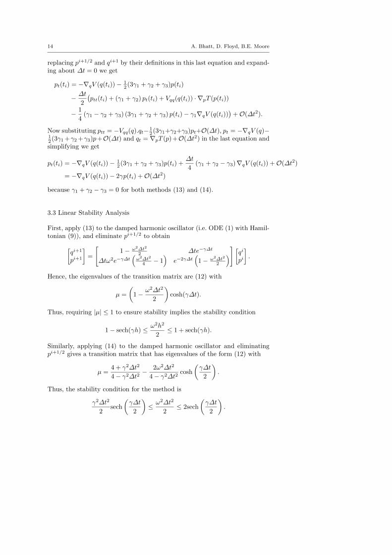
Figure 6 shows the norm of the difference between headings and corre-sponding entries of the table 2. This difference is less than the machine preci-sion as expected. Innermost planets (Jupitar ans Saturn) spiral into the Sunand the rest of the planets are in orbits which are fast converging toward theSun.

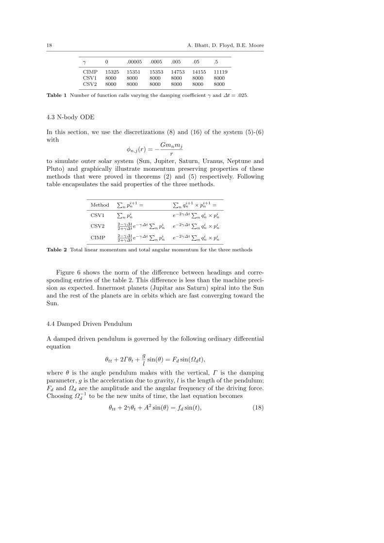
4.4 Damped Driven Pendulum

A damped driven pendulum is governed by the following ordinary differentialequation

θtt + 2Γθt +g

lsin(θ) = Fd sin(Ωdt),

where θ is the angle pendulum makes with the vertical, Γ is the dampingparameter, g is the acceleration due to gravity, l is the length of the pendulum;Fd and Ωd are the amplitude and the angular frequency of the driving force.Choosing Ω−1d to be the new units of time, the last equation becomes

θtt + 2γθt +A2 sin(θ) = fd sin(t), (18)


0 2000 4000

12345

x 10−21

t0 2000 4000

0

1

2x 10

−20

t

∆t = 10, γ = 0.0001, T = 5000

−10 0 10−20

−100

−10

−5

0

0 2000 4000

2

4

6

8

10

x 10−21

t0 2000 4000

0

1

2x 10

−20

t

−10 0 10−20

−100

−10

−5

0

0 2000 4000

12345

x 10−21

t0 2000 4000

0

2

4x 10

−20

t

−10 0 10−20

−100

−10

−5

0

CSV1

CSV2

CIMP

Fig. 6 Left to right: Error in linear momentum, error in angular momentum and corre-sponding planetary orbits.

with

γ = Ω−1d Γ, A2 = Ω−2dg

l, fd = Ω−2d Fd.

The sinusoidal term A2 sin(θ) in this equation is the one responsible for chaosin the system. In the numerical experiments that follow in this section, wewill discretize equation (18) with the numerical methods developed in earliersections and a second order RK (Heun’s) method and compare the numericalresults.

To this end, let us write equation (18) as a first order system

θt = ω,

ωt = −A2 sin(θ) + fd sin(t)− 2γω.(19)

Then a CIMP (7) based (implicit) method for this system is

γ/2Dγ/2t θ = γ/2A

γ/2t ω + γ γ/2A

γ/2t θ,

γ/2Dγ/2t ω = −A2 sin(γ/2A

γ/2t θ) + fd sin(Att)− γ γ/2Aγ/2t ω.

(20)


A CSV (15) based (explicit) method for this system is

(1 + γ1∆t/2)ωi+1/2 = e−γ3∆t/2ωi +∆t

2

(−A2 sin(θi) + fd sin(ti)

),

(1− γ1∆t/2)θi+1 = e−γ1∆t/2[(1 + γ1∆t/2)e−γ1∆t/2θi +∆tωi+1/2

],

eγ2∆t/2ωi+1 = e−γ1∆t/2[(1− γ1∆t/2)ωi+1/2 +

∆t

2

(−A2 sin(θi+1) + fd sin(ti+1)

)](21)

which gives a CSV1 based method on setting γ1 = 0, γ2 = 2γ, γ3 = 2γ and aCSV2 based method on setting γ1 = γ, γ2 = 0, γ3 = γ. Finally Heun’s methodfor this system is

ωi+1/2 = ωi +∆t(−A2 sin(θi) + fd sin(ti)− 2γωi

),

θi+1 = θi +∆t

2(ωi + ωi+1/2),

ωi+1 = 12 (ωi + ωi+1/2) +

∆t

2

(−A2 sin(θi +∆tωi) + fd sin(ti+1)− 2γωi+1/2

).

(22)

Figure (7) gives an example of a bounded orbit which is neither periodic norconvergent. In figure (8), we try to reproduce chaotic behavior of the systemas in figure (7) with a smaller ∆t. This figure shows the failure of Heun’smethod to reproduce the chaotic orbit as in figure (7) whereas other methodssuccessfully do so.

5 Time-Stepping Schemes for PDEs

To further analyze the methods discussed thus far, we apply them to PDEs,derive conformal properties that are preserved by the methods, and comparetheir performance numerically. Define space grid size by ∆x and xn = x1 +(n − 1)∆x, n = 1, 2, 3, . . . ,M , where x1 = −L, xM = L for x ∈ [−L,L]. Letzn,i denote the numerical approximation of z(xn, ti).

5.1 A damped Klein-Gordon equation

Consider a damped Klein-Gordon equation

utt = uxx − cu− 2γut, (23)

on the interval [−π, π] with periodic boundary conditions, whose exact solutionis taken to be

u(x, t) = e−γt cos(Kx−Wt), W =√K2 + c− γ2 (24)


0 500 1000−5

0

5

10

t

θ

−5 0 5 10−5

0

5

θ

ω

A = 1.5, γ = 0.375, ∆t = 2π/100, T = 1000, f = 4.7

−2 −1 0 1 2 3−4

−3

−2

−1

θ

ω

0 500 1000−5

0

5

10

t

θ

−5 0 5 10−5

0

5

θ

ω

−1 0 1 2 3−4

−3

−2

−1

θ

ω

0 500 1000−5

0

5

10

t

θ

−5 0 5 10−5

0

5

θ

ω

−1 0 1 2 3−4

−3

−2

−1

θ

ω

0 500 1000−5

0

5

10

t

θ

−5 0 5 10−5

0

5

θ

ω

−1 0 1 2 3−4

−3

−2

−1

θ

ω

CIMP

Heun’s

CSV2

CSV1

Fig. 7 Left to right: time series, phase space and Poincare sections of damped drivenpendulum (18) with the parameter values mentioned in the title. T is the final time.

0 500 1000−10

0

10

t

θ

−5 0 5 10−5

0

5

θ

ω

A = 1.5, γ = 0.375, ∆t = 2π/22, T = 1000, f = 4.7

−2 −1 0 1 2 3−4

−2

0

θ

ω

0 500 1000−10

0

10

t

θ

−5 0 5 10−5

0

5

θ

ω

−2 −1 0 1 2 3−4

−2

0

θ

ω

0 500 1000−10

0

10

t

θ

−5 0 5 10−5

0

5

θ

ω

−2 −1 0 1 2 3−4

−2

0

θ

ω

0 500 1000−10

0

10

t

θ

−5 0 5 10−5

0

5

θ

ω

−2 −1 0 1 2 3−4

−2

0

θ

ω

CIMP

Heun’s

CSV1

CSV2

Fig. 8 Left to right: time series, phase space and Poincare sections of damped drivenpendulum (18) with the parameter values mentioned in the title. T is the final time. Acomparison with figure (7) shows that Heun’s method cannot predict chaos with smaller∆t.


where K is the wavenumber and W is called the frequency of the wave. Thedissipation in the solution is −γ. This equation arises in relativistic mechanicsand has been discussed extensively in research literature, including [4,15].

One can rewrite equation (23) in conformal Hamiltonian form as

ut = v, vt = −(cu− uxx)− 2γv. (25)

We can also write the PDE (23) in conformal multi-symplectic form [15]

−vt − wx = cu+ 2γv

ut − px = v

−pt + ux = −w + 2γp

wt + vx = −cp

which can be written in short as

Kzt + Lzx = ∇Sγ(z)− γKz (26)

with

K =

0 −1 0 01 0 0 00 0 0 −10 0 1 0

, L =

0 0 −1 00 0 0 −11 0 0 00 1 0 0

, z =

uvwp

,where Sγ(z) = 1

2

(2γ(uv + wp) + v2 − w2 + cu2 − cp2

).

5.1.1 Numerical Solutions

Using the central finite difference operator

δ2un,i =un+1,i − 2un,i + un−1,i

∆x2,

we discretize the PDE (25) using (13) and (14) to get

vn,i+1/2 = e−γ∆tvn,i +∆t

2

(δ2 − c

)un,i,

un,i+1 = un,i +∆tvn,i+1/2,

vn,i+1 = e−γ∆t[vn,i+1/2 +

∆t

2

(δ2 − c

)un,i+1

],

(27)

and

(1 + γ∆t/2)vn,i+1/2 = e−γ∆t/2vn,i +∆t

2

(δ2 − c

)un,i,

(1− γ∆t/2)un,i+1 = e−γ∆t/2(

(1 + γ∆t/2)e−γ∆t/2un,i +∆tvn,i+1/2),

vn,i+1 = e−γ∆t/2(

(1− γ∆t/2)vn,i+1/2 +∆t

2

(δ2 − c

)un,i+1

),

(28)


respectively. Discretizing the PDE (26) in space with the implicit midpointmethod and in time with CIMP (7) gives the following scheme:

K(γ/2Dγ/2t Axz) + L(γ/2A

γ/2t Dxz) = ∇Sγ(Ax

γ/2Aγ/2t z). (29)

Figure 9 shows the absolute error in numerical solutions produced by (27),(28) and (29), where the exact solution is propagated with numerical fre-quency. Notice that the three numerical solutions are slightly out of phasewith each other due to their different numerical frequencies. Notice also thatthe error decreases for all three methods as time increases, primarily becausethe solution is dissipating to zero, but the relative error remains close to 10−2.

−3 −2 −1 0 1 2 3

1

2

3

x 10−11

x

Abs

olut

e E

rror

∆t = 0.025, ∆x = π/40, T = 50, γ = 0.375, c = 1, K = 8

−3 −2 −1 0 1 2 3

2468

x 10−9

x

Abs

olut

e E

rror

∆t = 0.025, ∆x = π/40, T = 40, γ = 0.375, c = 1, K = 8

−3 −2 −1 0 1 2 3

0.51

1.52

2.5

x 10−7

x

Abs

olut

e E

rror

∆t = 0.025, ∆x = π/40, T = 30, γ = 0.375, c = 1, K = 8

CSV1CSV2CIMP

Fig. 9 Error in the solution of (23) due to (27), (28) and (29). Parameter values are givenin the figure title. The maximum value of the exact solution at time T = 50 is approximately7 × 10−9.

Following the approach of [15] consider the function

d(t) = ln

(max

x∈[−π,π]u(x, t)

)+ γt (30)

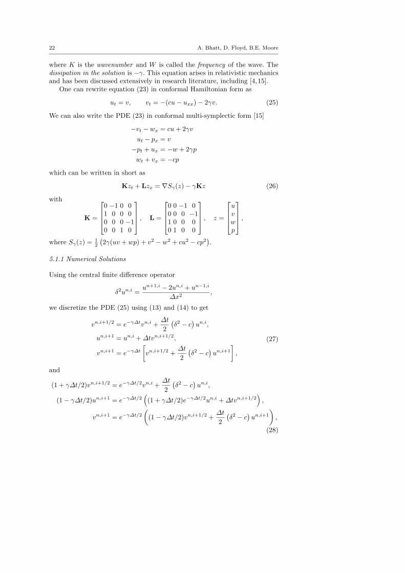
for measuring the drift in the rate of dissipation for the Klein-Gordon equation.Figure 10 shows no drift in the rate of dissipation (30) for the three methods.


0 5 10 15 20 25 30 35 40 45

−0.08

−0.07

−0.06

−0.05

−0.04

−0.03

−0.02

−0.01

0

∆t = 0.025, ∆x = π/40, γ = 0.375, c = 1, K = 8

t

Drift

CIMPCSV2CSV1

Fig. 10 Drift in the rate of dissipation for the three methods (27), (28) and (29) with theparameter values mentioned in the figure title. Only every sixth drift vector component isplotted for clarity and CSV1 eclipses CSV2.

5.1.2 Structure-Preservation

Consistent with the theme of this article, these methods preserve more thanconformal symplecticity, which helps explain the practical advantages of themethods. To be specific, define the momentum for the Klein-Gordon equation(25) by

I(t) =

∫ π

−πutux dx. (31)

Under appropriate boundary conditions, it can be shown that the PDE satisfiesthe conformal property

I(t) = e−2γtI(0). (32)

In fact, all three methods preserve this property.

Theorem 7 The numerical methods (27), (28) and (29) each preserve (32).

Proof Notice that

(1 + γ1∆t/2)vn,i+1/2 = e−γ3∆t/2vn,i − ∆t

2(cun,i − δ2un,i),

(1− γ1∆t/2)un,i+1 = e−γ1∆t/2[(1 + γ1∆t/2)e−γ1∆t/2un,i +∆tvn,i+1/2

],

eγ2∆t/2vn,i+1 = e−γ1∆t/2[(1− γ1∆t/2)vn,i+1/2 − ∆t

2(cun,i+1 − δ2un,i+1)

],

gives method (27) on setting γ1 = 0, γ2 = 2γ, γ3 = 2γ and method (28) onsetting γ1 = γ, γ2 = 0, γ3 = γ. Using these equations,

∑fnδgn = −

∑δfngn

and∑δ2fnδfn = 0 for any periodic sequences fn and gn, where

δfn =fn+1 − fn−1

2∆x,


we see that∑vn,i+1δun,i+1 = e−(γ1+γ2)∆t/2(1− γ1∆t/2)

∑vn,i+1/2δun,i+1

= e−(3γ1+γ2)∆t/2(1 + γ1∆t/2)∑

vn,i+1/2δun,i

= e−(3γ1+γ2+γ3)∆t/2∑

vn,iδun,i

= e−2γ∆t∑

vn,iδun,i

for both methods.Also notice that the equation (29) can be re-written as

(γ/2Dγ/2t )2A2

xu−D2x(γ/2A

γ/2t )2u = (γ2 − c)A2

x(γ/2Aγ/2t )2u

where A2xu = AxAxu etc. Now observe that, using Lemmas 1 and 2,

0 = γDγt

∑γ/2D

γ/2t A2

xu · δγ/2A

γ/2t A2

xu

=∑

(γ/2Dγ/2t )2A2

xu · δ(γ/2A

γ/2t )2A2

xu

+∑

γ/2Dγ/2t

γ/2Aγ/2t A2

xu · δγ/2D

γ/2t

γ/2Aγ/2t A2

xu

=∑(

D2x(γ/2A

γ/2t )2u+ (γ2 − c)A2

x(γ/2Aγ/2t )2u

)δ(γ/2A

γ/2t )2A2

xu

=∑(

D2x(γ/2A

γ/2t )2u

)δ(γ/2A

γ/2t )2A2

xu

because∑D2xU · δA2

xU =1

4∆x2

∑(Un+2 − 2Un+1 + Un) · δ(Un+2 + 2Un+1 + Un)

=1

2∆x2

∑Un+2δUn+1 +

1

4∆x2

∑Un+2δUn

− 1

2∆x2

∑Un+1δUn+2 − 1

2∆x2

∑Un+1δUn

+1

4∆x2

∑UnδUn+2 +

1

2∆x2

∑UnδUn+1

=1

∆x2

∑Un+2δUn+1 − 1

∆x2

∑Un+1δUn = 0

where we have used∑fnδgn = −

∑δfngn for any periodic sequences fn and

gn. Therefore, P i+1 = e−2γ∆tP i for

P i =∑

γ/2Dγ/2t A2

xun,i · δ γ/2Aγ/2t A2

xun,i.

We define the residual ri as

ri = ln

(Ii+1

Ii

)+ 2γ∆t,


0 10 20 30 40 50

−100

−10−5

−10−10

t

Ii

∆t = 0.025, ∆x = π/40, γ = 0.375, c = 1, K = 8

0 10 20 30 40

−1.5

−1

−0.5

0

0.5

1

1.5

2

2.5

x 10−15

t

ri

CIMPCSV1CSV2

CIMPCSV1CSV2

Fig. 11 Total conformal momentum Ii and residual ri due to (27), (28) and (29) with theparameters mentioned in the figure title

where

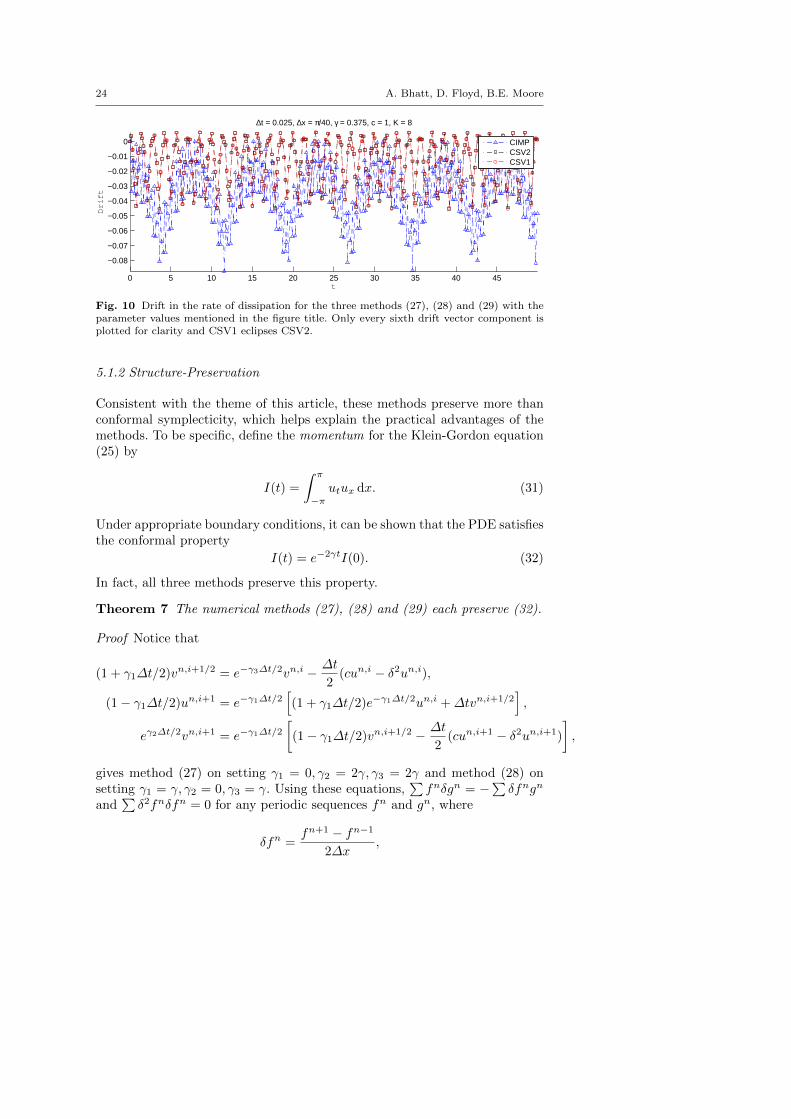
Ii =∑n

vn,iδun,i and Ii =∑

γ/2Dγ/2t A2

xun,i · δ γ/2Aγ/2t A2

xun,i,

for Stormer-Verlet type methods (27), (28) and implicit midpoint type method(29) respectively. Upon plotting Ii alongside respective residuals ri for thethree methods (27), (28) and (29), one obtains Figure 11, verifying momentumconservation properties of the methods. (Only some of the vector componentsare plotted to prevent overcrowding.)

5.2 A Modified Burgers’ Equation

Finally, consider application of the methods to a nonlinear equation, which werefer to as a modified Burgers’ equation, given by

ut + uux = −2γu, (33)

on the interval [−π, π] with periodic boundary conditions.

5.2.1 Numerical Solutions

To test our methods on this nonlinear problem, we discretize the space x ∈[−L,L], L = π, by introducing a uniform spatial grid [x1, x2, . . . , xM ] withgridsize ∆x such that x1 = −L, xM = L and M is even. Then we approximateu by un = u(xn), n = 1, 2, . . . ,M , with periodic boundary conditions un+M =un, and define the following vectors.

v = [u1, u3, u5, . . . , uM−1]T and w = [u2, u4, u6, . . . , uM ]T .


Discretizing equation (33) in space gives the following system of ODEs

dwn

dt= −∂+x ((vn)2/2)− 2γwn,

dvn

dt= −∂−x ((wn)2/2)− 2γvn,

(34)

where ∂+x and ∂−x are one-half of standard forward and backward difference op-erators, respectively, with periodic boundary conditions, for n = 1, 2, . . . ,M/2.Even-odd splitting of the dependent variable u was suggested in [3], andthis is the approach used here. Notice that the system is in the form znt =D∇znH(zn)− 2γzn with

D =

[0 ∂−x∂+x 0

],

which is constant and skew-symmetric, zn = [vn, wn]T andH(zn) = − 16 ((un)3+

(vn)3). Using method (14) to discretize time in system (34) we get the followingmethod

wn,i+12 = e−γ∆twn,i − ∆t

2∂+x

(vn,i)2

2,

vn,i+1 = e−γ∆t

e−γ∆tvn,i −∆t∂−x(wn,i+

12

)2

2

,

wn,i+1 = e−γ∆t(wn,i+

12 − ∆t

2∂+x

(vn,i+1)2

2

).

(35)

Equation (33) can also be put in multi-symplectic form

Kzt + Lzx = ∇S(z)− 2γKz

with

K =

0 0 −10 0 01 0 0

, L =

0 0 00 0 −10 1 0

, z =

uvw

and S(z) = −uv + u3

3 . If we now discretize this system in space with implicitmidpoint scheme and in time with (7) we get the following method

K(γDγtAxz) + L(γAγtDxz) = ∇S(Ax

γAγt z), (36)

which is equivalent to a two-step method

γAγtγDγ

tA2xu+ 1

2γAγtDx (Ax

γAγt u)2

= 0.

An equivalent one-step method is

γDγtAxu+ 1

2Dx (γAγt u)2

= 0. (37)


Another discrete model that can approximate solutions of (33) is the fol-lowing non-standard finite difference method (NFDM) (cf. [12])

un,i+1 − un,i(1−e−2γ∆t

2γ

) + un,i(un,i+1 − un−1,i+1

∆x

)= −2γun,i (38)

which is able to exactly reproduce certain solutions of the equation. Since thismethod is, in some way, also structure-preserving, it provides an interestingcomparison to the comformal symplectic methods.

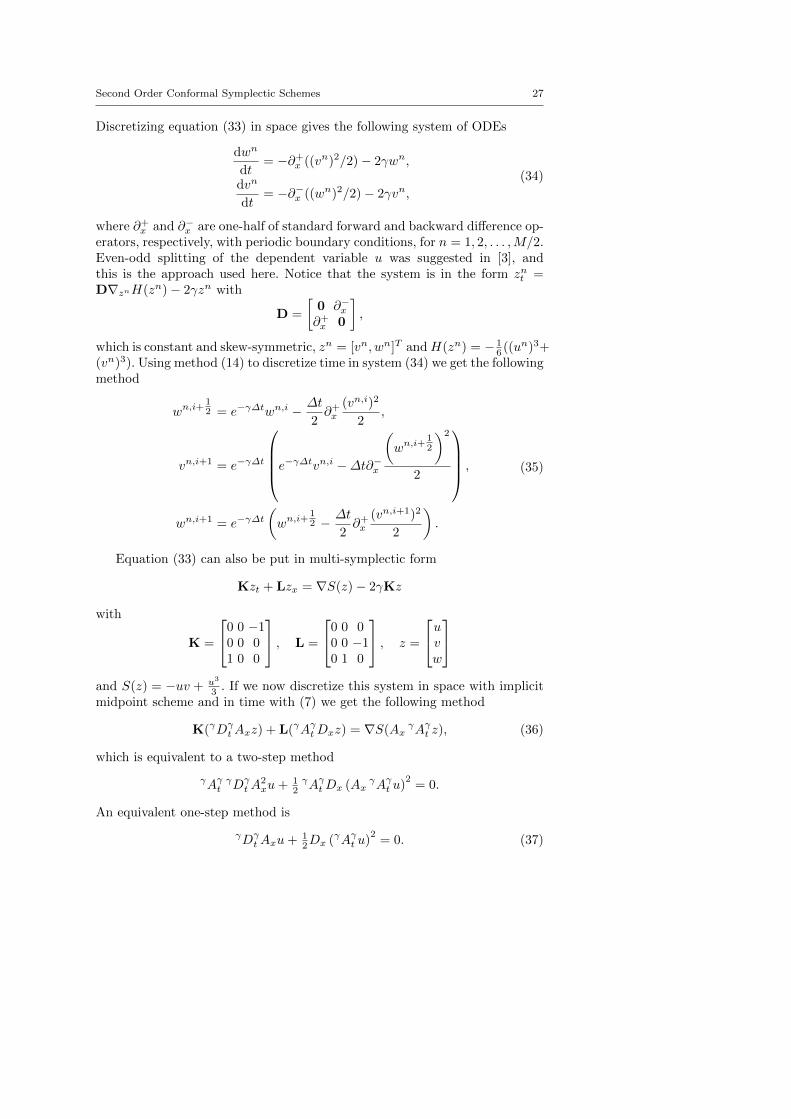
Numerical solutions of (33) at different times are given in Figure 12. Theinitial condition is taken to be a normal probability distribution function withmean 0 and standard deviation 1. As time progresses, the waveform becomessteeper, and the NFDM solution is damping at a different rate than the othertwo methods. In fact, the methods (35) and (37) are more accurate in thiscase, and the results of the following subsection explain how.

−3 −2 −1 0 1 2 3

0.1

0.2

0.3

∆t = 0.009, ∆x = 2π/79, γ = 0.25, T = 0

−3 −2 −1 0 1 2 3

2

4x 10

−3 ∆t = 0.009, ∆x = 2π/79, γ = 0.25, T = 8.991

−3 −2 −1 0 1 2 3

12345

x 10−12 ∆t = 0.009, ∆x = 2π/79, γ = 0.25, T = 49.995

un,i

1

x

CSV2CIMPNFDM

Fig. 12 Snapshots of the numerical solution of (33) using (35), (37) and (38) at differenttimes.

5.2.2 Structure-Preservation

Consider the Casimir

C[u] =

∫udx (39)

which corresponds to mass of the wave at time t and is an integral of motionfor the equation (33) with γ = 0. Differentiating (39) with respect to t, we


havedC

dt=

∫utdx = −

∫uuxdx− 2γ

∫udx.

Now using integration by parts and periodic boundary conditions we get∫ π

−πuuxdx = uu

∣∣∣∣π−π−∫ π

−πuxudx, =⇒

∫ π

−πuuxdx = 0.

ThereforedC

dt= −2γC ⇐⇒ C(t) = C(t0)e−2γ(t−t0), (40)

which is a conformal property of (33).

Theorem 8 Methods (35) and (37) preserve (40), but (38) does not.

Proof Casimir function (39) can be approximated by Ci =∑n u

n,i. Formethod (35), we get

Ci+1 =

M∑n=1

un,i+1 =

M/2∑n=1

(vn,i+1 + wn,i+1

)=

M/2∑n=1

e−2γ∆t(vn,i + wn,i

)= e−2γ∆tCi,

i.e. method (35) preserves (40). Summing equation (37) over the spatial indexn, we get∑

n

γDγtAxu = 0, =⇒

∑n

Axun,i+1 = e−2γ∆t

∑n

Axun,i,

=⇒∑n

un,i+1 = e−2γ∆t∑n

un,i,

i.e. method (37) also preserves (40). Similarly, summing (38) over the spatialindex n we get

2γ

1− e−2γ∆t∑n

un,i+1 =2γ

1− e−2γ∆t∑n

un,i − 2λ∑n

un,i

− 1

∆x

∑n

(un,iun,i+1 − un,iun−1,i+1),

which implies∑n

un,i+1 = e−2γ∆t∑n

un,i − 1− e−2γ∆t

2γ∆x

∑n

(un,iun,i+1 − un,iun−1,i+1).

Therefore, method (38) does not preserve (40).


To measure the error in (40) we define the residual ri

ri = ln

(Ci+1

Ci

)+ 2γ∆t, (41)

which is plotted in Figure 13, verifying that the conformal symplectic methodspreserve dissipation of mass, but NFDM does not.

0 20 40

10−8

10−6

10−4

10−2

100

Ci

∆t = 0.009, ∆x =2π/79, γ = 0.25

t0 20 40

−1

−0.5

0

0.5

1

x 10−15

ri

t0 20 40

−5

−4.5

−4

−3.5

−3

−2.5

−2

−1.5

−1

−0.5

x 10−5

ri

t

CSV2CIMPNFDM

Fig. 13 Left: Dissipation in total mass Ci. Middle: Residual (41) for the conformal sym-plectic methods (35) and (37). Right: Residual (41) for NFDM (38).

6 Conclusion

Numerical methods for solving damped Hamiltonian systems have been con-sidered in detail. The methods are based on Stormer-Verlet and implicit mid-point methods, which are commonly used for solving conservative equations.The methods have been constructed in a way that maintains second orderaccuracy, and they are called conformal symplectic, because they preserve theconformal symplectic structure of the systems. The fact that these conformalsymplectic methods also preserve many other dissipative properties of the gov-erning equations is a major theme of this work. To be specific, we have foundthat the methods preserve the rate of dissipation in the solution for linearequations; in the case of explicit schemes this result requires that the stepsize is sufficiently small relative to the damping coefficient. In addition, themethods preserve dissipation in momentum and mass for some special cases ofODEs and PDEs. Applying the methods to several model problems, in addi-tion to numerical comparisons to a higher order method and another structurepreserving method, demonstrate the strengths and advantages offered by con-formal symplectic methods.


References

1. F. Armero, I. Romero, On the formulation of high-frequency dissipative time-steppingalgorithms for nonlinear dynamics. I. Low-order methods for two model problems andnonlinear elastodynamics, Comput. Methods Appl. Mech. Eng. 190:2603-2649 (2001).

2. F. Armero, I. Romero, On the formulation of high-frequency dissipative time-stepping algorithms for nonlinear dynamics. II. Second-order methods, Comput. MethodsAppl. Mech. Eng. 190:6783-6824 (2001).

3. U.M. Ascher, R.I. McLachlan, Multi-symplectic box schemes and the Korteweg-de Vriesequation, Appl. Numer. Math. 48:255–269 (2004).

4. A. Eden, A. Milani, B. Nicolaenko, Finite dimensional exponential attractors for semi-linear wave equations with damping, J. Math. Anal. Appl. 169:408-419 (1992).

5. D. Furihata, Finite difference schemes for ∂u∂t

=(∂∂x

)αδGδu

that inherit energy conserva-

tion or dissipation property, J. Comp. Phys. 156:181-205 (1999).6. C. Kane, J.E. Marsden, M. Ortiz, M. West, Variational integrators and the Newmark

algorithm for conservative and dissipative mechanical systems, Int. J. Numer. Meth. Eng.49:1295-1325 (2000).

7. X. Kong, H. Wu, F. Mei, Structure-preserving algorithms for Birkhoffian systems,J. Geom. Phys. 62:1157-1166 (2012).

8. T. Matsuo, D. Furihata, Dissipative or conservative finite-difference schemes for complex-valued nonlinear partial differential equations, J. Comp. Phys. 171:425-447 (2001).

9. R.I. McLachlan, M. Perlmutter, Conformal Hamiltonian systems, J. Geom. Phys. 39:276–300 (2001).

10. R.I. McLachlan, G.R.W. Quispel, What kinds of dynamics are there? Lie pseudogroups,dynamical systems and geometric integration, Nonlinearity 14:1689–1705 (2001).

11. R.I. McLachlan, G.R.W. Quispel, Splitting methods, Acta Numer. 11:341–434 (2002).12. R.E. Mickens, Nonstandard Finite Difference Models of Differential Equations, pp. 185-

186. World Scientific, Singapore (1994).13. K. Modin, G. Soderlind, Geometric integration of Hamiltonian systems perturbed by

Rayleigh damping, BIT Numer. Math. 51:977-1007 (2011).14. B.E. Moore. Conformal multi-symplectic integration methods for forced-damped semi-

linear wave equations, Math. Comput. Simulat. 80:20-28 (2009).15. B.E. Moore, L. Norena, C. Schober, Conformal conservation laws and geometric inte-

gration for damped Hamiltonian PDEs, J. Comp. Phys. 232:214-233 (2013).16. H. Su, M. Qin, Y. Wang, R. Scherer, Multi-symplectic Birkhoffian structure for PDEs

with dissipation terms, Phys. Lett. A 374:2410-2416 (2010).17. Y. Sun, Z. Shang, Structure-preserving algorithms for Birkhoffian systems, Phys. Lett. A

336:358-369 (2005).

second order conformal symplectic schemes for … · second order conformal symplectic schemes for...

Documents