Hitotsubashi University Repository

Title Multi-Factor Flexible Budgeting

Author(s) Itami, Hiroyuki

CitationHitotsubashi journal of commerce and management,

10(1): 13-30

Issue Date 1975-05

Type Departmental Bulletin Paper

Text Version publisher

URL http://doi.org/10.15057/7442

Right

MULTI-FACTOR FLEXIBLE BUDGETlNG

By HIROYUKI ITAMI*

I. Introduction

For the purpose of cost control (through evaluating the coat performance of the mana-

ger), the standard cost and fiexible budgets system of direct costs and overhead cost have

been developed in the area of cost accounting over many years. These systems are con-sidered to be integral parts of the broader system, the system of responsibility accounting.

Or, in other words, standard costs and flexible budgets are supposed to be outcomes of

operational translations of the principle of responsibility accounting. The major question

that is asked in this paper is whether these translations and their outcomes are perfect or

good enough under all or most circumstances. Our answer on which we shall elaborate

in this paper is, "No, in some important circumstances." We further ask here whether it is possible or desirable to have a new operational translation of the principle of responsi-

bility accounting, and if so what that new system should look like as a new operational

system of cost control.

Considering that the standard cost system for control of direct costs is a part of the

over-all fiexible budgeting system, we propose here a multi-factor fiexible budgeting system,

as opposed to a single-factor flexible budgeting in the traditional standard cost and fiexible

budgets system. In this way we believe we can serve better or translate better the principle

of responsibility accounting for cost control. We have to add that our proposed system

does not concern with the product costing aspect which is one of the important aspects of

the standard cost system. Our main concern is the cost control through better (or more

appropriate or fairer) performance evaluation.

To further pursue this goal, we also attempt to search for new concepts of analysis

of variances which will be helpful in evaluating different aspects of abilities that are required

of the manager. Thus operational concepts of planning and supervisory variances emerge.

II. Flexible Budgeting in the Responsibility Accounting Framework

In the cost accounting literature, flexible budgeting (or budgets as its products) is

usually, though not necessarily, associated with the control of overhead cost and defined

as a set of different budgets which is keyed to different levels of operations, (Horn-

* Lecturer (Ko~shi) of Management science.

14 HITOTSUBASHI JOURNAL OF CO*MMERCE AND MANAGEMENT [May gren [4], p. 199.)

or Flexible budgets reflect the amount of cost that is reasonably necessary to achieve

each of several specified volumes of activity. (Shillinglaw [8], p. 373.)

Underlying these definitions of fiexible budgets is the implicit assumption that factors

other than levels of operations or volumes of activity remain approximately the same or

change, if any, only as the level of operations change, or do not affect the cost behavior

throughout the period flexible budgets are supposed to serve. Under these circumstances

we can concentrate our attention only to levels of operations in order to get the right kind

of budgets. (See Heckert and Wilson [3], p. 83.) It is this implicit assumption of conven-

tional and widely used flexible budgets that we would like to question in this paper. We

hasten to add that our research is not an empirical one to see whether there are any other

substantially infiuencial factors of cost behaviors on top of the levels of operations, but

rather a normative one to propose extentions of flexible budgeting with a single dominant

factor to multi-factor flexible budgeting in the framework of responsibility accounting,

when there are other factors to be considered in arriving at budget standards. Although

flexible budgets can be used as a tool for planning, their major uses seem to be for cost

control. In particular, we would like to stress and explore to its fullest extent the role of

flexible budgets as a tool for performance evaluation of the manager in charge of operations

for which fiexible budgets are prepared. As such the guiding principle for its preparation

is clearly laid down in the philosophy of responsibility accounting. To quote Horngren

again,

Each orgamzation unit of responsibility is budgeted on its contro!lable costs. Each

phase of operations is evaluated, and a prediction is made of how much cost should

be incurred under efficient conditions. The total of controllable costs is the line

manager's budgets. ([4], p. 31. Underlined by the author.)

Key words here are clearly responsibility, controllable costs, and efficient conditions.

With these key concepts in mind, Iet us now examine whether traditional fiexible budgets

measure up to this guiding principle. When we speak of flexible budgets in this paper,

we take them rather broadly to include not only overhead costs but also direct labor and

material costs, which are usua]ly considered to be completely variable with levels of ope-

rations. One of the reasons for doing so is. that in traditional standard ･cost system direct labor and material costs can be considered completely flexible (1inearly changing) parts

of over-all flexible cost budgets, the factors of proportionality being the standard costs

per unit output and the level of operation being the number of the output produced.

Another reason is our suspicion that 'standard unit labor cost or material cost' may not

be that standard and constant. Quite often these standard costs are determined as the

'best attainable' costs assuming some normal level of activity under normal circum~tances.

In those cases, 'best attainable' unit costs for labor and material might change as surround-

ing conditions change. This implies that we may not take direct labor and material costs

just as linear functions of output levels. The factors of proportionality of these linear

functions themselves may well change if we apply the idea of 'best attainable' unit cost

rather stringently under every circumstance. The following example might help_ clarify

some pomts. Suppose the manager has two processes (or activities) to produce product A, Ptocess

l 975] 15 MULTI-FACTOR FLEXIBLE BuDGETING

l uses 5.5 units of labor and 7 units of material and Process 2 consumes 4 and 8 of' each,

respectively. Each process produces a ton of product A. By machine-hour limitations,

the manager cannot operate Process I more than 500 units. The similar limitation for

Process 2 is 300. Suppose that normal conditions mean that the output level is 600 tons

of Product A, and prices are $1 for one unit of labor and $2 for one unit of material. Tech-

nologically speaking, there is no dominance between Process I and Process 2. Cost condition will decide which or what combinations of two is the best under normal condi-

tions. Unit process costs for I and 2 are $19.5 and $20 respectively. Therefore it is easy

to see that the best combination of two processes under normal conditions is 500 units of

Process I and 100 units of Process 2, thus making standard cost for labor per ton of output

(5.5X500+4X 100) / 600=~'5.25 and standard cost for material per ton of output 2 (7X

500+8XIOO) / 600=$14.33. Standard labor requirement per ton of output is 5.25 and standard material requirement is 7.17 per ton of output. If the actual production volume

is 700 tons of Product A, similar calculations show the best attainable cost for labor per

ton of output is $5.07 and for material $14.57.

This example clearly shows that even if the underlying production processes are linear

processes, the cost structure might not be linear with respect to output levels when there are

alternative production processes and some limitations on the scale of each process.

If we are to consider these cases carefully, we have to incorporate direct labor and

material costs into our flexible budgeting scheme as total costs, not as unit costs. In this

way we can allow nonlinearity to creap even into direct costs. Let us now see there are

situations where we need more factors other than production levels as the deternilnants of

suitable budgets for performance evaluation even under this rather broad concept of traditional flexible budgeting.

Suppose, in the previous example, the material price changes rather frequently from

period to period and the manager can know the price for the material he is going to use for

a period at the beginning of the period. Suppose the material price happens to be $1.4 at

the beginning of a particular period. Then, unit process costs for Process I and Process

2 are ~15.3 and $15.2. Now it is better to use Process 2 up to the limit, 300, and then use

Process I for the rest of production. Thus, changes in material prices can cause the change

of minimum-cost technology and therefore cause a change in the whole structure of flexible

budgets, if we take them as best attainable budgets under changing circumstances. To make these points clear, the following table is set up for best attainable costs under various

circumstances and corresponding standard costs calculated using standard labor and material cost per unit of production, $5.25 and $14.33. x denotes the output level, and

c2 denotes material price. Standard labor and material requirements are calculated by

using 5.25 and 1.77, standard requirements at normal conditions.

In Table 2, case 3, standard material cost is calculated using c2=1.4, not c2=2, so that we

TABLE I . LABOR

Case Standard Labor cost Standard labor Labor quantity quantity cost - l. x600, ca2

2. x700, cs:=2 3, x=:600, c2 := I . 4

3 1 50

3550

2850

3 1 50

3675 3 1 50

3 1 50

3550

2850

3 1 50

3675 3 1 50

16 HITOTSUBASHI JOURNAL OF COMMERCE AND MANAGEMENT

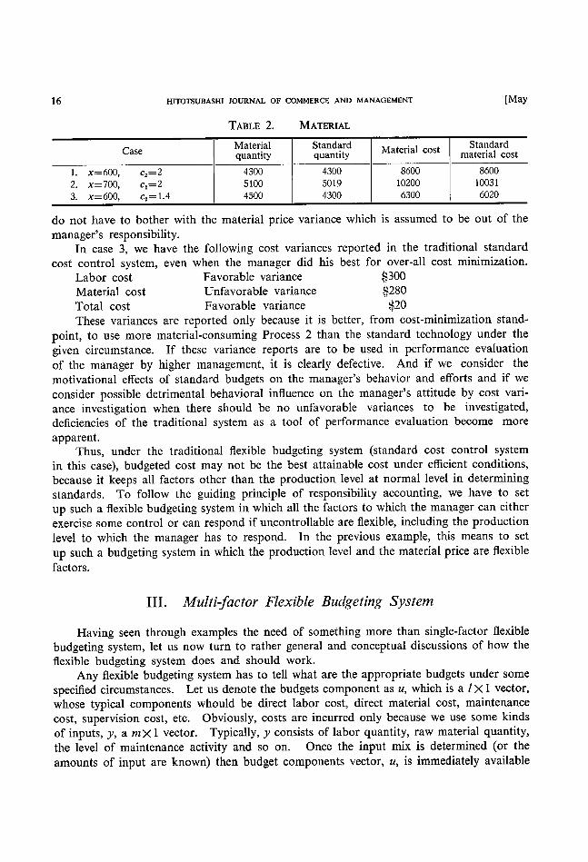
TABLE 2. MATERIAL

[May

Case

1 , x= 600, c2 =; 2

2, x =: 700, c2 == 2

3. x=600, c2 = I . 4

Material quantity

4300

5100

4500

Standard quantity

4300 5019

4300

Material cost

8600

10200

6300

Standard material cost

8600 l 003 l

6020

do not have to bother with the material price variance which is assumed to be out of the

manager's responsibility.

In case 3, we have the following cost variances reported in the traditional standard

cost control system, even when the manager did his best for over-all cost minimization.

$300 Favorable variance Labor cost $280 Unfavorable variance Material cost ~20 Favorable variance Total cost

These variances are reported only because it is better, from cost-minimization stand-

point, to use more material-consuming Process 2 than the standard technology under the

given circumstance. If these variance reports are to be used in performance evaluation

of the manager by higher management, it is clearly defective. And if we consider the

motivational effects of standard budgets on the manager's behavior and efforts and if we

consider possible detrimental behavioral influence on the manager's attitude by cost vari-

ance investigation when there should be no unfavorable variances to be investigated,

deficiencies of the traditional system as a tool of performance evaluation become more

apparent. Thus, under the traditional flexible budgeting system (standard cost control system

in this case), budgeted cost may not be the best attainable cost under efficient conditions,

because it keeps all factors other than the production level at normal level in determining

standards. To follow the guiding principle of responsibility accounting, we have to set up such a flexible budgeting system in which all the factors to which the manager can either

exercise some control or can respond if uncontrollable are flexible, including the production

level to which the manager has to respond. In the previous example, this means to set

up such a budgeting system in which the production level and the material price are flexible

factors.

III. Multi- actor Flexible Budgeting System fi

Having seen through examples the need of something more than single-factor flexible

budgeting system, Iet us now turn to rather general and conceptual discussions of how the

flexible budgeting system does and should work. Any fiexible budgeting system has to tell what are the appropriate budgets under some

specified circumstances. Let us denote the budgets component as u, which is a I X I vector,

whose typical components whould be direct labor cost, direct material cost, maintenance

cost, supervision cost, etc. Obviously, costs are incurred only because we use some kinds

of inputs, y, a m X I vector. Typically, y consists of labor quantity, raw material quantity.

the level of maintenance activity and so on. Once the input mix is determined (or the

amounts of input are known) then budget components vector, u, is immediately available

1 975] MULTI-FACTOR FLEXIBLE BuoGETING 17 as the function of input amounts, y, and their prices, c, I Xm vector. That is,

(1) u =f(c, y) , where f is a vector-valued function.

Given the production output quantities the manager has to produce x, a n X I vector.

the input mix required to produce x depend on many parameters of production process(es)

and input prices, c, when the cost minimization is sought. Let us divide the totality of

these parameters into two subsets, a, P･ Division into two subsets in done considering the manager's responsibility and controllability with respect to each of parameters.

First, a is a vector of those parameters to which the manager cannot exercise any

control, Iike material price in the previous example, or unknown yield on some raw mate-

rials. p is a vector of those parameters to which he can maintain some degree of control,

like labor productivity which he can influence, for example, through efforts for good human

relations. Since the input mix, y, is treated as the basic decision vector here, which es-

sentially covers the area of production planning, kinds of control the manager has over

p might be termed supervisory control, most of them of behavioral nature. Given the production goal x, the values of uncontrollable parameters, a, the manager has to decide

and implement some production plan, y, in one way or other, assuming that levels of controllable parameters, P, are determined somewhere independently from input mix planning. Thus, input levels, y, can be considered a function (vector-valued) of x, a, p as

follows.

(2) y=ip (x, a, ~) By substituting y for (1), we get

u =f (c, (x, a, P))

Since c is considered to be included in a or / and p,

(3) u=ip (x, a, ~) The implicit assumption in the traditional flexible budgeting that we mentioned earlier

in the paper is the same thing as a particular assumption about the functional form of (2)

and (3) used in establishing the standards. It implicitly says that in arriving at standards

of performance evaluation, we can set a and p to their standard values d, ~ and then find

out y's and u's for changing x's. By so doing it actually omits a and ~ from the significant

arguments in the function c and therefore ~)-Since, the purpose of fiexible budgets is just to establish the standards, not to calculate

the actual amount of y's and u's necessary in various situations, this simplication might be

good enough in some circumstances. For example, when the production process is rigid

enough so that we do not have any choice in production planning other than just to obey

the technology of the production process in producing a given x, it might be better to ac-

count non-standard cost behavior due to deviations of a and p from the standards as variance due to a and variances due to P and then focus our attention on variances due to

p, since it is these latter controllable variances that are the focal points of cost control

efforts under this circumstance.

In other circumstances, Iike in the previous example, where there are several alternative

production processes and levels of some of a should have substantial effects on the pro-

duction planning itself (like different choices of processes depending on the material price

in the previous example) the approach of the traditional fiexible budgeting will leave very

important part of the manager's performance evaluation obscured, that is, the evaluation

18 mTOTSUBASHI JOURNAL OF COMMERCE AND MANAGEMENT [May of his planning ability, by not taking into account those responses deemed necessary on

the part of the manager to changes of some of a from their standards. It seems important here to distinguish two different kinds of uncontrollable parameters,

a. One group consists of those uncontrollable parameters to which the manager can respond in the production planning phase, called a, here, and the others are those to which

the manager cannot respond in the production planning phase but just has to accept their

consequences passively in the production implementation phase, a2'

Differences between al' and a2, might become clear if we consider the availability of

information with respect to levels of al' and a2, m a particular period. Should the manager

be able to know what value an uncontrol]ab]e parameter will take in a particu]ar period

before he starts implementing the production plan for the period, thus enabling him to

make plans suitable for the known value of the parameter, this parameter is one of al. If

the value of a parameter is not available beforehand but available only after the fact, this

is one of a2'1

With this refinement, (2) and (3) can be rewritten as follows

(4) y=q,! (x, al, a2, p)

(5) u=ip (x, al' a2, P) (4) is a quantity budget and (5) is a cost budget. Any flexible budgeting system can be

considered as a special case of (4) and (5), differing in the functional form of ~,f and ~ and

the treatment of x, al, a2, p. For example, in the traditional single-factor fiexible budgets,

x is somehow reduced to a scalar and the nature of ip and ~9 is determined considering

'efiicient' cost behavior under normal conditions and effects of different values of al' are

ignored. Also all the al' a2 and p, are set to their standard values.

What we would like to propose here is a new flexible budgeting scheme, flexible not

only over x,2 but also over al'

Making budgets flexible over some parameters implies that the manager is released

from the responsibility about the values of those parameters themselves but in return is

charged of responding in an appropriate manner to changes of these parameter values.

Release of responsibility for parameter values is justified because al is assumed to be un-

controllable, and new charge for appropriate response is exactly in line with the philosophy

of responsibility accounting and would be helpful in the evaluation of the manager's plan-

ning ability. Coupled with the evaluation of the manager's supervisory abilitythr ough

cost variances due to P, new dimensions of performance evaluation would be possible by

establishing new variance analysis approach under this multiple-factor flexible budgeting

system. These topics will be treated in later sections in detail.

After setting down the general framework of a multi-factor flexible budgeting system,

two critical problems remain to be solved. First of all we have to determine, in each particular situation for which we apply this

general framework, what al' a2 and p are. It is difficult to discuss in general about this other than the definitions of al' a2 and p

which are given in the previous pages. Higher management is able to set al' a2 and p as

* n is possible that the line of demarkation between a*, and a, may not be clear~ut. In that case it is up to the particutar designing principle of the evaluation system to decide between a*, and a,.

' In case when x is multi-dimensional, fiexibility over x itself is already an extension over the single-factor

fiexible budgeting system.

1 975] MULTI-FACTOR FLEXIBLE BUDGETING 19 it sees fit for performance evaluation of lower management. In particular, a parameter

would have to satisfy at least the following two conditions to be included in al'

1 . The manager should be held responsible for responding to changes in the

parameter, and can do so in his production planning.

2. The parameter value changes rather frequently and its changes are believed

to have significant effects on the cost behavior under 'efficient conditions'.

Particularly interesting are the various factors which can be incorporated in a multi-

factor flexible budgeting system as x or al, and which are often neglected completely in the

traditional flexible budgeting system.

For example, when the activity and costs of the department in question has some interdependencies with those of other departments, cost standards for the department

should take into these interdependencies into account. As a more concrete example. suppose department A supplies a part of its outputs as an input into department B. If

department A has to adjust its production plan rather substantially as department B's

request for its intermediate goods changes, then the output level of this intermediate goods

should be included as an important component of x (maybe al' depending on the model formulation).

Another case in point is when there may exist a substantial "borrowing from the

future" Borrowmg from the future rs said to occur for example when the manager defers his maintenance work to the future periods so that he can have less cost in the pre-

sent period than otherwise, although the manager eventually has to pay for this deferment.

Whenever the borrowing from the future can be big enough to warrant careful attention

in the performance evaluation in the present period, intertemporal considerations have to be made either through suitably defining and relating some paraments of a, to the pre-

sent cost or defining some of x as the state of the system which will restrict future alternatives.

The second critical problem of a multi-factor flexible budgeting system is the derivation

of the functional form ~), or how to get the value of u=~) (x, al' a2, P) for each (x, al' (~2,

~) vector. One thing which is clear from the guiding principle' of responsibility accounting

is that the nature of ~ has to incorporate some kind of efficiency criteria. In this paper

we consider q, should represent the minimized (or optimum) cost, given x, al' Thus we

postulate some cost minimizing production planning model behind ~ and consider ~ to

trace optimal solutions for changing x, al.

As for the treatment of a2 and p in setting standards, we discuss it in the next and sub-

sequent sections. It is the purpose of the next section to see how we can determine ~p or

how we can build a production planning model suitable for a mu]ti-factor flexible budgeting

and then find u for each x and al under linear production processes.

IV. Linear Production Process: Activity Analysis Model

of Manufacturing Operations

Linear programming techniques have already been applied in budgeting in Stedry [9], and ljiri et al. [6] and so on. In this section we would like to propose to use a special

type of linear programming models as a planning and budgeting model, es~ecially~ ih

20 mTOTSUBAsm JOURNAL OF COMMERCE ANI) MANAGEMENT [May manufacturing operations. Such a model is based on the concepts of activity analysis

which has been developed mainly in the field of economics to treat the linear production

processes3 and can be used as a way of formulating the production planning model in Imear

programming context. As we shall see, this activity analysis model seems to be particularly

suitable as a basic model in a multi-factor flexible budgeting framework. We have to add

here that appllcations of activity analysis-type models in budgeting should not be limited

to manufacturing budgets but can be made in other areas of budgeting, financial budgets

etc.

One of the central concepts in activity analysis is 'activity' or 'process' with fixed

technological coefficients. Process I and Process 2 in the previous example are examples

of activities in this sense. Each activity consumes, at unit level of operation, certain

amounts of certain inputs, and produces certain amounts of certain outputs. These amounts are assumed not to change as the level of the activity changes. In this framework,

the problem of production planning is the problem of how to plan the activities levels so

that we can minimize the cost under certain constraints on activity levels. In the previous

example, inputs are labor, material, and the output is Product A. Constraints exist for

machine-hours. We call a vector of technological coefficients a technology vector. For

example,

Process I Process 2 (~

*)

'.' ,

"

l)

' * "

The first elements are output coefficients. The foruth elements of two vectors are machine-

hour requirements for machine I which is exclusively used for Process 1, thus zero entry in Process 2's vector. The fifth elemerrts are similar machine-hour requirement for machine 2.

If we denote the activity levels of Process I and 2 as zl' z2 and the total labor quantity

as yl' the total material quantity as y2, and the output level as x, the basic production

relationship is expressed by :

~ (1~ (x 1 ( )1 ~8) ~ ) 5.5 z+ 4 z= yl 7

y2

zl ~ 500

z2 ~ 300

zl' z2;~O

In the previous example, we assumed that costs would be incurred only for labor and material, not for machine-hours. (Machine cost is a fixed or uncontrollable cost in this

example.) Therefore, the production planning model with cost minimization objective

under normal conditions is

min. yl + 2y2 subject to above conditions

' See, for example, Koopmans (7).

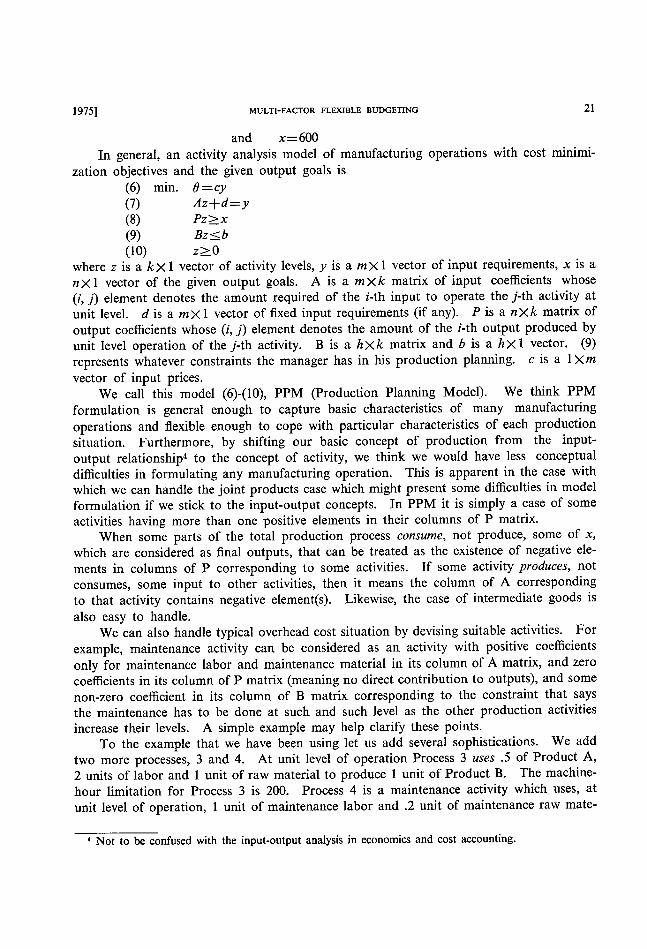
1975] MULTI-FACTOR FLEXIBLE BuoGmNc 21 and x 600

In general, an activity analysis model of manufacturing operations with cost minimi-

zation objectives and the given output goals is

(6) min. 0=cy

(7) Az+d=y (8) Pz~:x (9) Bz ~ b (10) z;~O

where z is a kX I vector of activity levels, y is a mX I vector of input requirements, x is a

nX1 vector of the given output goals. A is a mXk matrix of input coefficients whose (i, j) element denotes the amount required of the i-th input to operate the j-th activity at

unit level. d is a mX1 vector of fixed input requirements (if any). P is a nXk matrix of

output coefficients whose (i, j) element denotes the amount of the i-th output produced by

unit level operation of the j-th activity. B is a hXk matrix and b is a hXl vector. (9)

represents whatever constraints the manager has in his production planning. c is a I X m

vector of input prices.

We call this model (6)-(10), PPM (Production Planning Model). We think PPM formulation is general enough to capture basic characteristics of many manufacturing

operations and flexible enough to cope with particular characteristics of each production

situation. Furthermore, by shifting our basic concept of production from the input-output relationship4 to the concept of activity, we think we would have less conceptual

difficulties in formulating any manufacturing operation. This is apparent in the case with

which we can handle the joint products case which might present some difficulties in model

formulation if we stick to the input-output concepts. In PPM it is simply a case of some

activities having more than one positive elements in their columns of P matrix.

When some parts of the total production process consume, not produce, some of x, which are considered as final outputs, that can be treated as the existence of negative ele-

ments in columns of P corresponding to some activities. If some activity produces, not

consumes, some input to other activities, then it means the column of A corresponding

to that activity contains negative element(s). Likewise, the case of intermediate goods is

also easy to handle. We can also handle typical overhead cost situation by devising suitable activities. For

example, maintenance activity can be considered as an activity with positive coefficients

only for maintenance labor and maintenance material in its column of A matrix, and zero

coefficients in its column of P matrix (meaning no direct contribution to outputs), and some

non-zero coefficient in its column of B matrix corresponding to the constraint that says

the maintenance has to be done at such and such level as the other production activities

increase their levels. A simple example may help clarify these points.

To the example that we have been using let us add several sophistications. We add

two more processes, 3 and 4. At unit level of operation Process 3 uses .5 of Product A,

2 units of labor and I unit of raw material to produce I unit of Product B. The machine-

hour limitation for Process 3 is 200. Process 4 is a maintenance activity which uses, at

unit level of operation, I unit of maintenance labor and .2 unit of maintenance raw mate-

' Not to be confused with the input-output analysis in economics and cost accounting.

22 HrroTSUBASHI JOURNAL OF COMMERCE AND MANAGEMENT [May rial. It does not contribute to the production of any output directly, but let us suppose

.that z4, maintenance activity level, has to be such that

, Izl + ' 1 5z2 + '05z3 ~z4,

that is, the maintenance level has to increase as levels of Processes 1, 2 and 3 increase at

least at the rate of .1, .15, .05 respectively.

Now the formulation of this expanded example is as follows, assuming $1.2 for main-

tenance labor price and $1 for maintenance material price.

min. yl+2y2+ 1.2y3 + y4

( o :).,+(: .~f'=(~' ) y* y, '*+ '* +

o

o

o

2- 5z3;~xl zl+z . Z3 >_ x2

zl ~ 500 Z2 ~ 300

z3 ~ 200

. I zl + ' 1 5z2 + '05z3 = Z4 ~ O

z z z z>0 1' 2, 3, 4-y3 denotes the amount of maintenance labor, y4 the amount of maintenance material, xl

the given output goal for Product A, and x2 the given output goal for Product B.

As can be seen in this example, input variables, y, in PPM can be of substantial variety.

It is not difficult at all to have many different kinds of labor, many different kinds of mate-

rial, and other kinds of kinputs. This another capability of PPM formulation is additional

strength in budgeting where it might be desirable to split master budgets (e.g., master

budgets for labor) into smaller segments. For example, after knowing optimal levels of

z, y is just linear functions of z (y=Az+d) and,

(11) 2ciyi, L=a set of indices for all the labor inputs i=L

is the master labor budgets. Each ciyi, i e L, will give its breakdown.

Although PPM is formulated as a linear programming problem, nonlinearity of input

consumption or output production or in the constraints can be handle approximately by

using a piece-wise linear approximation of non-linear functions. For details of this for-

mulation, see ljiri [5]. In corporation of non-1inearity into PPM is very important if we

are to consider such cost elements as overhead-type costs, Iike step costs and semi-variable

costs.

Trivially, the case when the manager does not have any technological choice in alter-

native production processes in producing the given output goal x can be considered as a

special case of PPM. It is the case when the constraints (8) and (9) are strict enough to

allow only one solution or there is only one activity in the model (that is, k=1).

From the above arguments about the versatility of PPM as a basic production plan-

ing model, we consider we can use PPM in determi.ning multi-factor flexible budgets.

That is, we think PPM has three necessary characteristics as a basic model to be used

in a multi-factor fiexible budgeting system. First of all, most importantly, PPM can be

expected to represent manufacturing operations reasonably well, if not perfect. Secondly,

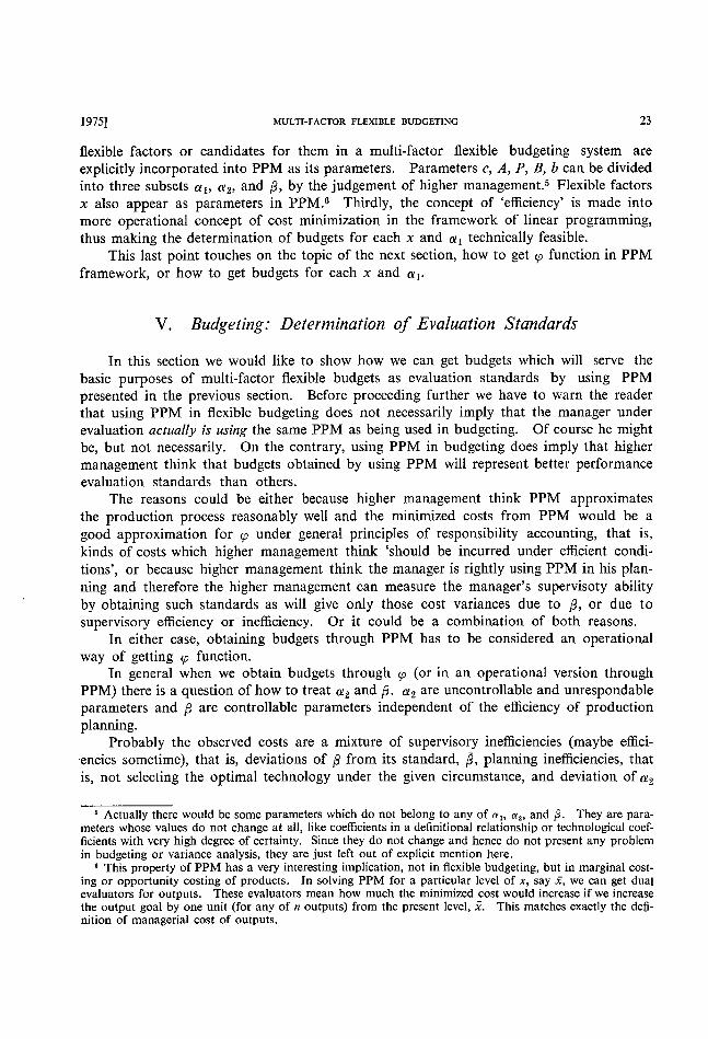
l 975] MULTI-FACTOR FLEXIBLE BUDGETlNG 23

flexible factors or candidates for them in a multi-factor flexible budgeting system are

explicitly incorporated into PPM as its parameters. Parameters c, A, P, B, b can be divided

into three subsets al' a2, and p, by the judgement of higher management.5 Flexible factors

x a]so appear as parameters in PPM.6 Thirdly, the concept of 'efficiency' is made into

more operational concept of cost minimization in the framework of linear programming,

thus making the determination of budgets for each x and al technically feasible.

This last point touches on the topic of the next section, how to get ~) function in PPM

framework, or how to get budgets for each x and al'

V. Budgeting: Deterlnination of Evaluation Standards

In this section we would like to show how we can get budgets which will serve the

basic purposes of multi-factor flexible budgets as evaluation standards by using PPM

presented in the previous section. Before proceeding further we have to warn the reader

that using PPM in flexible budgeting does not necessarily imply that the manager under

evaluation actually is using the same PPM as being used in budgeting. Of course he might

be, but not necessarily. On the contrary, using PPM in budgeting does imply that higher

management think that budgets obtained by using PPM will represent better performance

evaluation standards than others.

The reasons could be either because higher management think PPM approximates the production process reasonably well and the minimized costs from PPM would be a good approximation for ~ under general principles of responsibility accounting, that is,

kinds of costs which higher management think 'should be incurred under efficient condi-

tions', or because higher management think the manager is rightly using PPM in his plan-

ning and therefore the higher management can measure the manager's supervisoty ability

by obtaining such standards as will give only those cost variances due to ~, or due to

supervisory efficiency or inefficiency. Or it could be a combination of both reasons.

In either case, obtaining budgets through PPM has to be considered an operational

way of getting ~) function.

In general when we obtain budgets through p (or in an operational version through PPM) there is a question of how to treat a2 and ~, a2 are uncontrollable and unrespondable

parameters and p are controllable parameters independent of the efficiency of production

planning.

Probably the observed costs are a mixture of supervisory inefficiencies (maybe effici-

'encies sometime), that is, deviations of p from its standard, ~ , planning inefficiencies, that

is, not selecting the optimal technology under the given circumstance, and deviation of a2

5 Actually there would be some parameters which do not belong to any of al, az, and p . They are para-meters whose values do not change at all, Iike coefficients in a definitional relationship or technological coef-

ficients with very high degree of certainty. Since they do not change and hence do not present any problem in budgeting or variance analysis, they are just left out of explicit mention here.

6 This property of PPM has a very interesting implication, not in flexible budgeting, but in marginal cost-

ing or opportunity costing of products. In solving PPM for a particular level of x, say X, we can get dual evaluators for outputs. These evaluators mean how much the minimized cost would increase if we increase the output goal by one unit (for any of n outputs) from the present level, x. This matches exactly the defi-

nition of managerial cost of outputs.

24 HITOTSUBASHI JOURNAL OF COMMERCE AND MANAGEMl3NT [May from its standards, d2' Therefore, to get the right kind of evaluation standards that will

be capable of evaluating supervisory efficiency, it is clear that we have to set p to ~ so that

we can detect the deviation of ~ from ~ and its effects on costs by observing the actual costs

and comparing them with appropriate standards. As for a2, we set them to d2 in obtaining

standards and then try to separate the uncontrollable part of observed cost variances con-

tributed by the deviation of a2 from ~22, because a2, are uncontrollable and unrespondable.

This implies that the manager may plan his production by using the standard values of a,

and then adjust his plan, rather passively because of the definition of a2 as the realized

values of a2 become known after starting the implementation of the original plan. The

problem of variance analysis will be treated in detail in the next section.

Thus the problem of a multi-factor flexible budgeting becomes how to get

(12) u p (x, al' d2, ~) operationally for different values of x and al'

In PPM, this is to solve a parametric programming problem, parametric in x, which is a part of the stipulation vector, and a 1, which may scatter over c, A, P, B, b, with a2 and

P set to a2 and p. Let us denote by A (al' d2, ~) A matrix in which a2 part and ~ part are set to d2, ~

and al are left as parameters. Similar meanings for c (al, d2, ~), P (al' d2, ~) and so on.

Now the parametric programming problem to be solved is (13) min. =c (al' d2, ~) y

(14) A (al' d2, ~) z+d (al' d2･ ~) =y (15) P (al' d2･ ~) z~:x (16) B (al' ~2, ~) z~b ((~l' d2, ~)

(17) z;~O. Let us call (13)-(17) BDM (Budget Determination Model).

Unfortunately techniques of parametric programming in linear programming are not

advanced enough to treat such a complicated parametric program as BDM. Therefore, the best we can hope is to actually solve BDM for each x and al' As evaluation standards,

we only have to solve BDM for a particular x and cel' materialized in a particular period

after the fact. If we want to obtain a multifactor flexible budget before the fact as a moti-

vational devise, then we would problably have to solve BDM for certain representative

values of x and al, and do some kind of approximation for other values of x and al' In

this context, certain interesting behaviors of objective values, O', might help. Denoting

by c (al) the al part of c and so on, the following remarks apply.

e', seen as a function of x and b (al)' is an increasing, piece-wise linear, convex

function of x and a decreasing, piece-wise linear, convex function of b (al)' e' is also

a concave function of c (al)'7

Once we get the optimal solution, z', for BDM for a particular value of x and al' budg-

eting itself becomes rather trivial. Let us denote this optimal solution by

z'=z' (x, al)

recognizing the fact that z' is a function of x and a 1' This determines the optimal combi-

nation of activities.

Then, the corresponding input mix is,

T proofs are in the appendix.

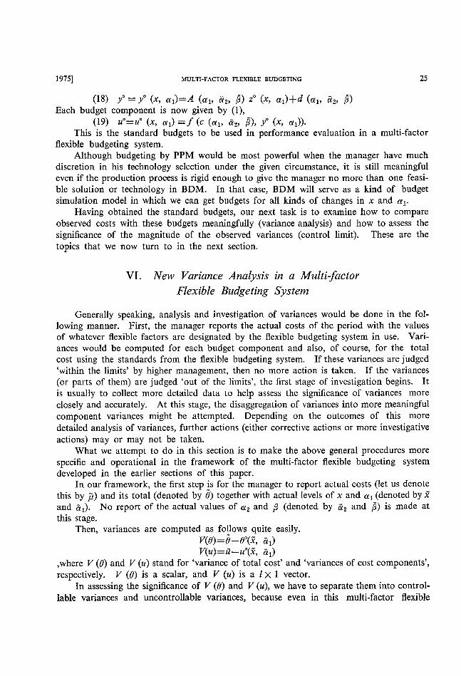
1975] MULTI-FACTOR FLEXIBLE BUDGETING 25 (18) y y (x a ) A (al' d2, ~) z' (x, al)+d (al' d2, ~)

Each budget component is now given by (1),

(19) u'=u' (x, al) =f(c (al, d2, ~), y' (x, al))'

This is the standard budgets to be used in performance evaluation in a multi-factor

fiexible budgeting system.

Although budgeting by PPM would be most powerful when the manager have much discretion in his technology selection under the given circumstance, it is still meaningful

even if the production process is rigid enough to give the manager no more than one feasi-

ble solution or technology in BDM. In that case. BDM will serve as a kind of budget

simulation model in which we can get budgets for all kinds of changes in x and al'

Having obtained the standard budgets, our next task is to examine how to compare observed costs with these budgets meaningfully (variance analysis) and how to assess the

significance of the magnitude of the observed variances (control limit). These are the

topics that we now turn to in the next section.

VI. New Variance Analysis in a Multi actor -fi

Flexible Budgeting System

Generally speaking, analysis and investigation of variances would be done in the fol-

lowing manner. First, the manager reports the actual costs of the period with the values

of whatever flexible factors are designated by the flexible budgeting system in use. Vari-

ances would be computed for each budget component and also, of course, for the total

cost using the standards from the flexible budgeting system. If these variances are judged

'within the limits' by higher management, then no more action is taken. If the variances

(or parts of them) are judged 'out of the limits', the first stage of investigation begins. It

is usually to collect more detailed data to help assess the significance of variances more

closely and accurately. At this stage, the disaggregation of variances into more meaningful

component variances might be attempted. Depending on the outcomes of this more detailed analysis of variances, further actions (either corrective actions or more investigative

actions) may or may not be taken. What we attempt to do in this section is to make the above general procedures more

specific and operational in the framework of the multi-factor flexible budgeting system

developed in the earlier sections of this paper.

In our framework, the first step is for the manager to report actual costs (let us denote

this by p) and its total (denoted by O) together with actual levels of x and al (denoted by j~

and dl)' No report of the actual values of a2 and ~ (denoted by az and ~) is made at

this stage.

Then, variances are computed as follows quite easily.

V(e)=6-e'(~, ~l) V(u)=ti-u'(~, al)

,where V (6) and V (u) stand for 'variance of total cost' and 'variances of cost components',

respectively. V (6) is a scalar, and V (u) is a I X I vector.

In assessing the significance of V (e) and V (u), we have to separate them into control-

lable variances and uncontrollable variances, because even in this multi-factor flexible

26 HITOTSUBASHI JOURNAL OF COMMERCE AND MANAGEMENT [May budgeting system u' (j~, al) does not account for the uncontrollable cost increase due to the

deviations of a2 from a2 8 and, in principle, we want to know controllable variances.

Without knowing i22, the assumption which is made at this stage, we have to determine

somehow whether there exist significant controllable variances in V (O) and V (u). Here

controllable variances mean variances due to planning inefficiencies or / and supervisory

inefficiencies (deviations of ~ from P)-

Although any way of disaggregating variances into the controllable part and the uncontrollab]e part would have some degree of arbitrariness, we think the following dis-

aggregation is reasonable.

Define p (x, al' ai2) and t (x, al' ~2) as component costs and total cost (counterparts

of u and O respectively) which would be incurred if the initial production plan is made as

z' (x, al) (which is determined at (~2=d2, ~ =~), but adjustments to activity levels, z', are

made during the period to cope with ~2 as they become known, that is, to satisfy the given

output goal, x, and the constraints under a2=d2, but keeping p at ~.

After having obtained the adjusted z, z/, costs are calculated as follows.

y/ A(al, a2' ~)z/+d(al, a2' ~) u=p(x, al, a2) = f(c(al' a2, ~), y/)

e=r(x, al, a2)=c(al, d2, ~)y!. Theref ore,

T(x, al, d2)=g'(x, al)

p(x, al, d2)=u'(x, al)'

because no adjustment are necessary if a2=i22'

Functions T and p are clearly dependent on how intraperiod adjustments are made.9

However these adjustments are made, we can conceptually define the uncontrollable vari-

ances, denoted by UCV (a) and UCV (u), and controllable variances, denoted by CV (O)

and CV (u), as follows.

(20) UCV(e)=c(j~, al' a2)~O'(j~, ~l)

(21) CV(e)=C-r(i, dl' a2) (22) UCV(u)=p(j~, al' a2)~u'(i, al)

(23) CV(u)=:a-p(~, al' d2)' Of course,

V(O) = UC V(e) + C V(O)

V(u) = UCV(u) + CV(u).

Notice, again, that by assumption we do not know (or have not done any investigation

to know) the values of a2 at this stage. Therefore, we do not know the values of 7 (x, al'

a2) and ,l (x, al, a2)' Only things we know are O, a, O' (i, dl)' and u' (~, al)' Suppose,

8 Although it is possible to get u' and C' from BDM using a, instead of i2,, resulting budget standards would be too much or too little to expect from the manager because, by definition, he cannot respond to any changes in a,, but getting budgets with d,, implies that he should respond optimaly to realized values of a,, thus making a,, the same fiexible factors as a* in their characteristics.

9 One example of intraperiod adjustments is the following. Use only those activities which are employed in z' (x, a*), (in the linear programming terminology, keep the same basis), and find an adjusted z to satisfy

the output goals and the constraints. If there are none of those z's we have to specify some way of changing

to or / and adding another set of activities. If there are more than one such z, then select the z, for example,

as close as possible to z' (x, a*), that is, with the minimum distance from z'. This refiects the often-advocated

principle of stay-close-to-the-original-plan. Instead of the minimurn distance criterion, we might impose the

minimum 'adjustment cost' criterion, which may complicate the problem more.

1975] ' MULTI-FACTOR FLEXIBLE BUI)GETING 27 however, we know the probability distribution of a2, denoted by p (a2)' Then, t and p

become random variables whose joint probability distribution function can be obtained

using p (~2) and T (~, i21' d2) and p (j~, al, d2)'

Let us denote this joint probability function by q (~, p).ro It is possible to get q (T,

p) operationaly, if tedious, because we know functions T and p, although we do not know

values of T and p for yet unknown values of a2' From here, it is just one step to get the joint probability distribution of CV (O) and

CV(u). Now we can get information on important probabilities in the following manner.

Pr(CV(O)=0, CV(u)=0)=q(e, u), Pr(CV(O)=0)= J~q(~, p)dp,

Pr(CV(u)=0)=J･q(r, a)df'

If these values are sufficiently large, say .80 or over, then we probably do not have to

investigate any further. If these probabilities are not large enqugh, say .80 or less, then

we would go ahead for further investigation.11

We can, of course, base our decision on other kinds of probabilities, Iike

Pr( CV(e)1 ~r)

or Pr (lCV (e) ~rl' and some component of CV(u)l~r2), where r, rl' and r2 are small positive numbers indicating higher management's judgement. In the latter example, higher

management is concerned on the controllable variances of the total cost and some com-

ponent cost they think important. Thus, having a joint probability distribution for CV

(O) and CV (u) is really helpful, and we can do a variety of statistical tests before we decide

to go ahead for further investigation.

As the second major stage of cost variance analysis, Iet us suppose higher management

have decided to investigate further and got information on i~2, ~･ Now we know the value of c (j~, a!1' a2) and p (~, al, a2)' Therefore values of CV (O) and CV (u) are known, too.

Now having the values of controllable variances, CV (O) and CV (u), it would be useful

if we can break CV (O) and CV (u) down so that we can see the causes of variances. In

particular, we are interested in disaggregating the controllable variances by two major

causes, planning inefiiciency and supervisory inefficiency.12 Each of these two is a very

important item in performance evaluation of the manager. Following the basic idea behind the derivation of lr and p, Iet us define lr (x, al' a2' p)

and I (x, al' d;, ~) as the total cost and component costs which would be incurred if the

initial production plan is made as z' (x, al)' but adjustments are made to activity levels,

z', during the period to cope with a2, and ~ as they become known, that is, to satisfy the

lo since functions T and p are hardly analytic functions, we may have to use the Monte Carlo simulation

technique to get q (r, p). ll Here, instead of these classical hypotheses-testing analysis (hypotheses being CV (e)=0 or CV (u)=0),

we might do Bayesian analysis. Or we can obtain the optimal investigation po]icy, assuming investigation

cost and benefit. See Dyckman (2). le Here we are assuming perfect implementation of the plan, perfect in the sense that actual activity levels

does not deviate at all from what the manager (or the planner) wants them to be. If there is any degree of imperfection in implementation, the terms planning inefficiency and planning variances should be interpreted

as meaning planning-implementation inefficiency and variance in the rest of this paper.

28 HITOTSUBASHI JOURNAL or COMMERCE AND MANAGEMENT [May given output goal, x, and the constraints under a2=a2, and p=~.13

Theref ore,

IT (x, al' a2, ~)=T (x, al' a2)

1 (x, al' a2, ~)=p (x, al' d2)'

The same remarks about the intraperiod adjustment mechanisms apply to lr and I as to

T and p. From the definitions of T, p, ~ and IF functions, it seems reasonable to define super-

visory variances (meaning cost variances due to supervisory inefficiency or efficiency) as

follows. They are denoted by SV (e) and SV(u), for the total cost and component costs respectively.

(24) SV(O)=T (j~, al' a2, ~)-T (X, al' ~2) (25) SV(u)=), (j~, al' ~2, ~)-p (j~, al' ~2)

We may likewise define planning variancesl4 (meaning cost variances due to planning

inefficiency), denoted by PV (O) and PV (u) respectively for the total cost and component

costs, as follows :

(26) PV(O)=0-1T (~, al' a2, p) (27) PV(u)=a-1 (j~, al' a2, p).

These definitions seem reasonable considering the meanings of IT and ~.

From (20)-(27) it is clear that

(28) CV(e)=SV(e)+pV(O) (29) CV(u)=SV(u)+pV(u).

Thus we have arrived at the desired disaggregation of controllable varinaces both

for the total cost and for component costs. Especially, (29) means quite something.

There, the complicated infiuence of supervisory and planning inefficiency is carefully in-

corporated into each component variances. Furthermore, such vague terms as planning ineffciency or supervisory inefficiency are now cast in cost terms having very concrete

meanings. They say, for exan]ple, if the manager supervises his operation (which affects

parameter values p) successfully and keeps them at their standards, the cost reduction would

be SV (O) dollars in total. In this sense, planning and supervisory variances presented

here may be considered as valuations of the manager's planning and supervisory in-effici-

ency (in gross terms) by opportunity costs. Being opportunity costs, they change their

values as surrounding conditions change, that is, as x and al change.

The importance of planning and supervisory variances in evaluating the manager's

over-all performance, not each specffic phase of his operation (like evaluation of each P),

is self-evident. Having obtained these two variances, it is now up to higher management

to decide how to assess their significance and how to act upon their assessment.

*3 In Demski (1), a seemingly similar but rather different concept of the ex post optimal program is in-troduced. His ex post optimal program is the optimal solution of the linear programming model with all the parameters having their actual values, not standard values. In our framework, it corresponds to z' (x. al) when all the parameters are treated as (rl, or a special intraperiod adjustment mechanism which yie]ds ex post optimal solution. See also the footnote in p. 23.

l' See the second footnote of the previous page.

l 975] MuLTI-FACTOR FLE)(IBLE BuoGETlNG 29

VII. Summary and Concluding Remarks

Summary and concluding remarks are now in order. In this paper we examined both the basic philosophy of responsibility accounting and

the current state of a single-factor flexible budgeting, and decided that in some situations

a single-factor flexible budgeting did not serve the purpose that it should, thereby creating

some need for a multi-factor flexible budgeting system.

After presenting a special type of linear programming models, called the activity

analysis model, as a basic model-type suitable for modeling manifacturing operations, we

noted that the activity analysis model (PPM) was particularly suitable as a basic model in

a multi-factor budgeting system.

Using PPM in budgeting, we could obtain a feasible system for multi-factor fiexible

budgeting and showed how to get budgets operationally.

New variance analysis using PPM framework and distinction among decision para-meters, uncontrollable and respondable parameters, al' uncontrollable and unrespondable

parameters, a2, and controllable parameters, p, resulted in a very interesting way of dis-

aggregating variances. First we indicated an operational way of separating uncontrollable

variances from controllable ones. Further disaggregation of controllable variances lead

to the notions of planning variances and supervisory variances, which would be impor-

tant pieces of information in evaluation of the manager's over-all performance.

Thus, we have laid down the conceptual as well operational framework for a multi-

factor flexible budgeting system.

And now the following discussions of merits and demerits of the proposed multi-factor

flexible budgeting system are in order.

In this system, the manager is held responsible when he does not take the opportunity

of profitting from the favorable environment (favorable al) and he is excused when the

environment turns hostile to him (unfavorable al)' In this sense he will be given fair per-

formance evaluation in line with the idea of responsibility accounting. Whatever good

motivational effects the fair evaluation may have on the attitude of the manager should

certainly be credited to the merits of the system. In this regard, careful selection of al by

higher management becomes very important. Another obvious merit of this proposed system is that it will save unnecessary cost variance investigation which would be done in

the traditional system. That is the investigation of those variances due to al which will

be costly as well as unfruitful and even detrimental (probably) to the manager's motivation.

There is also an obvious demerit in this new system. That is, the difficulty of interium

reports and evaluation during the period. As can be seen easily from the mechanism of

budget determination in this new system, we do not have any evaluation standards until

the end of the period when we start calculating standard budgets using BDM.

True and net merits of a multi-factor fiexible budgeting system are yet to be seen in

practical terms. Their empirical evaluation as well as the elaboration of the proposed

system in much greater detail would be topics for further research.

30 HlTOTSUEASm』0URNAL　OF　COMM旧RCl…AND　MAN＾G］≡MENT

　　　　　　　　　　　　　　　　　　　　　　■RE冊REWCE∫

1．Demski，J．，“An　Accounting　System　Structured　on　a　Linear　Programming　Mode1，”

　Z加■cco〃〃加g1～〃加w，42（4），0ctober1967，pp．701－712．

2．Dyckman，T．，“The　Analysis　of　Cost　Variances，”■o〃川α1gグ■㏄o〃〃伽g沢ωωκん，7

　（2），Fa111969，PP．215－244・

3，H㏄kert，J．and　J，Wi1son，肋3加∬肋伽肋gα〃Co〃o1，3rd　ed．，New　York：The　Rona1d　Press，1967．

4．Homgren，C、，Co〃■㏄o〃〃肋g’ノ〃伽αgε肋1五㎜ψα3加，Englewood　Cli価s，N．J．：　Prentice＿壬Ia11．　1962．

5．Ijiri，Y．，〃o〃αgε㎜ε〃Goα13α〃■㏄o〃〃肋g力7Co〃ro1，Amsterdam：North－Hol1and，

　1965．

6．Ijiri，Y．，F．Levy　and　R．Lyon，“A　Linear　Programming　Model　for　Budgeting　and

　Financia1P1anning，”Jo〃閉o1げ■㏄o〃〃肋g1～ω8〃cん，1（2），A11tumn1963，pp．198－212．

7－Koopmans，T．，ed．，ん伽妙ルo伽f∫ψ〃o∂“c〃o〃伽∂ノ〃oco〃o〃，New　York：John　Wi1ey，1951．

8．Shi1lingIaw，G．，Co並ノ㏄o〃〃加gjノ〃o伽た伽∂Co〃ro1，2nd　ed、，Homewood，I11．：

　Richard　Irwin，1967．

9．Stedry，A．，肋砲αCo〃rol　o〃Co∫ご肋乃〃for，Englewood　Cli冊s，N．J．：Prentice－HaH，

　1960．