hmc and all that - bu blogs – blogs for the boston...

IntroductionWhat is HMC good for?

Pseudofermions and RHMCSymplectic Integrators

Non-Renormalizability of HMCConclusions

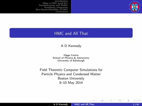
HMC and All That

A D Kennedy

Higgs CentreSchool of Physics & Astronomy

University of Edinburgh

Field Theoretic Computer Simulations forParticle Physics and Condensed Matter

Boston University8–10 May 2014

A D Kennedy HMC and All That 1 / 20

THE

UNIVERSI T

Y

OF

E D I N B U RGH




HMC: The MovieHMC: The Algorithm

What does HMC stand for?

Video by Tamara Broderick (Berkeley) and DavidDuvenaud (Cambridge)https://www.youtube.com/watch?v=Vv3f0QNWvWQ

Hans Christian Andersen, Molecular dynamicssimulations at constant pressure and/or temperature,J. Chem. Phys., 72, 2384 (1980).P. J. Rossky, J. D. Doll and H. L. Friedman,Brownian dynamics as smart Monte Carlo simulation,J. Chem. Phys., 69, 4628, (1978).

HMC is a Markov Chain Monte Carlo(MCMC) algorithm.

It is widely used in Lattice FieldTheory, Machine Learning, and severalother fields.It was originally called Hybrid MonteCarlo.

Based on the Hybrid algorithm ofDuane and Kogut (a hybrid ofMolecular Dynamics and amomentum heatbath).Made “exact” by Metropolis MonteCarlo accept/reject step.

In the statistics and machine learningfields it is called Hamiltonian MonteCarlo, which is probably a moremeaningful name.


THE

UNIVERSI T

Y

OF

E D I N B U RGH





What is HMC?

HMC introduces a “fictitious” Hamiltonian H(q, p) = T (p) + V (q) definedon the “positions” (or fields) q and a set of equally fictitious momenta p.The kinetic energy is chosen to be T = p2/2 (changing the coefficient isequivalent to rescaling time).

It constructs an ergodic Markov Chain with the fixed-point distributione−H over the phase space (q, p).It does this by alternating two steps

Selecting new momenta from a Gaussian heatbath, leaving the positionunchaged.Approximately integrating Hamilton’s equations for a reasonably long timeτ using an integrator that is exactly reversible and area-preserving (such asleapfrog), and then performing a Metropolis accept/reject step.Both steps have e−H as their fixed point distribution, but they are certainlynot ergodic individually.


THE

UNIVERSI T

Y

OF

E D I N B U RGH





Cost and Tuning

The fictitious momenta have nothing to do with any physical momenta inthe system. People sometimes try to use the “real” Hamiltonian dynamicsinstead, but it is not clear why this should be advantageous.

In free field theory the optimal trajectory length is of the order of thecorrelation length of the field theory under study. Both theoretical analysisand empirical measurements indicate that using shorter trajectories is afalse economy.

When the Hamiltonian is extensive, so using an integrator which has errorsof O(δτ n) requires V δτ n to be held constant. The volume scaling of thecost is therefore V 1+1/n at fixed trajectory length = correlation length.For leapfrog n = 4, so the cost grows as V 5/4 independent of thedimension of the lattice.

For large volumes using higher order symplectic integrators becomesworthwhile, but this makes the parameter-tuning problem harder.


THE

UNIVERSI T

Y

OF

E D I N B U RGH




What is HMC good for?

What problems doesn’t it solve?Sign problems: i.e., when there are huge cancellations between differentregions of the integration region.Such sign problems can be solved by reformulating the theory, but this isvery model-dependent (no general solution).There are interesting results using the complex Langevin algorithm (but I donot really understand why).Is there a suitable algorithm for a Quantum Computer?

What problems does it solve?It reduces autocorrelations.There is a large reduction in cost for interacting theories compared withLangevin or other small step or local update methods.For free field theory it reduces the dynamical critical exponent z from 2 to 1.For interacting theories this is also true in practice, even if perhaps not intheory (more later. . . ).


THE

UNIVERSI T

Y

OF

E D I N B U RGH




FermionsIntegrator InstabilitiesMultiple PseudofermionsRHMC

Fermions

In principle we could keep track of the sign and explicitly integrate overGrassmann-valued fields. The problem is that the resulting integral has a“sign problem”.

For renormalizable field theories (without too much improvement) fermionfields only occur quadratically in the action, and can be integrated to givethe determinant of the discrete Dirac operator.

〈Ω〉 ∝∫

dU dψ dψΩ(ψ, ψ,U)e−S(U)−ψM(U)ψ ∝∫

dU detM(U) Ω(U)e−S(U)

with

Ω(U) =

[Ω

(δ

δη,δ

δη,U

)e ηM

−1(U)η

]η=η=0

,

where the fermion kernelM = /D + m (or (/D + m)†(/D + m) in practice).

The determinant is real and positive, detM = det γ5Mγ5 = detM†.


THE

UNIVERSI T

Y

OF

E D I N B U RGH





Pseudofermions

We can replace the determinant withan integral over pseudofermion fieldswith kernelM−1,

〈Ω〉 ∝∫

dU d φ dφ Ω(U)e−S(U)−φM−1(U)φ.

For heavy fermions this works well, butfor light fermions the step size δτ → 0in order to accept anything.

For a long time this was thought to bedue to large fermionic forces comingfrom “exceptional” gauge fieldbackgrounds (“blame the usualsuspects”).


THE

UNIVERSI T

Y

OF

E D I N B U RGH





Integrator Instability

But this was not the case. The culprit was that we are using a singlepseudofermion field to estimate the fermionic force, and it is therefore verynoisy.

The Markov process still has the correct fixed point distribution even whenthe integrator becomes unstable, but the autocorrelation becomes zerobecause nothing is accepted.

The fundamental problem is that the large fluctuations in the estimator ofthe fermionic force cause the gauge field integrator to become(exponentially) unstable.

The solution is to use several pseudofermions to estimate the fermionicforce.

Ideally, each of the n pseudofermions should each contribute contributedetM1/n to the functional integral.


THE

UNIVERSI T

Y

OF

E D I N B U RGH





Multiple Pseudofermions

There are several ways of doings this

Hasenbusch: several pseudofermions with larger masses.Several cheap heavier pseudofermions plus a more costlycorrection term to ensure the correct determinant.

Lüscher: domain decomposition. Partition lattice into evenand odd blocks together with a “small” residual correction,each with their own pseudofermions. For light enoughfermions the residual part will domainate.

Rational HMC (RHMC): use rational approximation forM1/n. Requires thesolution of a large linear system for each pole in the rational approximationfor each pseudofermion.

In practice some combination of the techniques usually works best.


THE

UNIVERSI T

Y

OF

E D I N B U RGH





RHMC

RHMC makes use of multishift Krylov space solvers.

It is remarkable that all the coefficients in the Chebyshev optimal rationalapproximation x1/n ≈

∑j

αj

x+βjare positive, so the method is numerically

stable.

Usually only two or three pseudofermions are required, and 10 to 20 polesare required to achieve full floating-point accuracy over the spectrumofM.

Using these simple tricks the integrator step size can be increased byabout an order of magnitude before the fermionic force (rather than thenoise of its estimator) causes the instability to be triggered.

This has allowed lattice QCD computations to be carried out at thephysical π mass, thus eliminating the need for chiral perturbation theoryextrapolation in the mass.

“I expect chiral perturbation theory to apply below the pion mass”

— Jürg GasserA D Kennedy HMC and All That 10 / 20

THE

UNIVERSI T

Y

OF

E D I N B U RGH




Symplectic SymmetrySymplectic IntegratorsShadows

Symplectic Structure

Hamiltonian systems have an innate symplectic symmetry.Consider the exterior derivative of the Lagrangian

dL(q, q) =∂L

∂qdq +

∂L

∂qdq =

d

dt

(∂L

∂qdq

)=

d

dt(p dq)

using the Euler–Lagrange equations and defining p ≡ ∂L/∂q.Hence d2L = 0 requires that the fundamental 2-formω ≡ −d(p dq) = dq ∧ dp is time independent (Darboux theorem). It mustalso be closed, dω = 0.

This allows us to associate a vector field A with any 0-form (function) Aon phase space, dA(X ) = ω(A,X ) for any vector field X .

A is called a Hamiltonian vector field, even if A is not the Hamiltonian.

Classical trajectories are integral curves of H, where H is the Hamiltonian.


THE

UNIVERSI T

Y

OF

E D I N B U RGH





Poisson Brackets

The definition of the exterior derivative of a 0-form is dA(X ) = X A, hence

A B = dB(A) = ω(B, A) ≡A,B

where

A,B

is the Poisson bracket

of two phase space functions. ClearlyA,B

= −

B,A

.

According to Jacobi (1840)«. . . quelques remarques sur la plus profonde découverte de

M. Poisson, mais qui, je crois, n’a pas été bien comprise ni parLagrange, ni par les nombreux géomètres qui l’ont citée, ni parson auteur lui-même.»

For non-Francophones we may thank Google for the following translation“. . . a few remarks on the most profound discovery of Mr.

Fish, which, I think, was not well understood by either Lagrangeor by many others who have cited it, nor by the author himself.”


THE

UNIVERSI T

Y

OF

E D I N B U RGH





Jacobi Identity

The definition of the exterior derivative of a 2-form is

dω(X ,Y ,Z) = Xω(Y ,Z) + Yω(Z ,X ) + Zω(Y ,X )

−ω([X ,Y

],Z)− ω(

[Y ,Z

],X )− ω(

[Z ,X

],Y )

where[X ,Y

], the commutator of two vector fields, is iteself a vector field.

For Hamiltonian vector fields Aω(B, C) = −AB,C

= −

A,B,C

.

Moreover, ω([A, B

], C) = −ω(C ,

[A, B

]) = −dC(

[A, B

]) =

−(AB− BA)C = −AB,C

+ B

A,C

= −

A,B,C

+B,A,C

.

Combining these we find that Poisson brackets satisfy the Jacobi identityA,B,C

+B,C ,A

+C ,A,B

= 0.

Hence functions on phase space form a Lie algebra with the Poissonbracket as the Lie product.


THE

UNIVERSI T

Y

OF

E D I N B U RGH





BCH Formula

Using the Jacobi identity we find that[A, B

]C =

A,B, C

−B,A, C

=

A, B, C

=A,B

C for

all C , so we get the remarkable result that commutator of two

Hamiltonian vector fields is a Hamiltonian vector field:[A, B

]=A,B

.

The Baker–Campbell–Hausdorff (BCH) formula (due to F. Schur,according to Bourbaki) states that eAeB = eC where C =

∑n≥1 Cn with

C1 = A + B and

(n+1) Cn+1 = − adCn(A−B)+

bn/2c∑m=0

B2m

(2m)!

∑k1,...,k2m≥1k1+···+k2m=n

adCk1 . . . adCk2m(A+B),

where Bn are Bernoulli numbers and (adX) Y =[X,Y

].

For Hamiltonian vector fields this gives eAeB = eC where C =∑

n≥1 Cn

where the Cn are 0-forms given by the same formula, but this time forfunctions rather than vector fields and with (adA) B =

A,B

.


THE

UNIVERSI T

Y

OF

E D I N B U RGH





Integrators

Remember that classical trajectories were integral curves of theHamiltonian Hamiltonian vector field. For H(q, p) = T(p) + V(q) (forparticle physics V = S) we have, at least locally where ω = dq ∧ dp,H = T + S where T = T′(p) ∂

∂q and V = −V′(q) ∂∂p .

We cannot integrate H exactly, but We can construct an exact discreteintegrator for T

eδτTf(q, p) =∑n≥0

δτnT′(p)n

n!

∂nf∂qn (q, p) = f

(q + T′(p)δτ, p

)

using Taylor’s theorem, and likewise for eδτVf(q,p) = f(q, p−V′(q)δτ

).

This only converges for small enough δτ , of course.

In fact it is really only an asymptotic expansion: if we consider theevolution of the probability distribution e−H(q,p) of phase space points,then q or p may be arbitrarily large with exponentially small probability.


THE

UNIVERSI T

Y

OF

E D I N B U RGH





Shadow Hamiltonians

Using the BCH formula we may construct integrators for H to any desiredorder in the step size δτ .

What is perhaps more surprising is that this integrator, while it onlyapproximately conserves H, exactly conserves a nearby ShadowHamiltonian H, namely that built out of Poisson brackets using the BCHformula.

The first application of this result is that HMC trajectories conserveenergy to O(δτn) for arbitrarily long trajectory lengths, becauseH(q, p)−H(q, p) = O(δτn) everywhere in phase space.


THE

UNIVERSI T

Y

OF

E D I N B U RGH





Tuning HMC

Our second application is that we can use theShadow to tune the parameters of oursymplectic integrator.

The idea is that the Poisson brackets occuringin the BCH formula are extensive quantities,and therefore average to constants.

We therefore perform one HMC run andmeasure all the relevant Poisson brackets, wethen minimize the variance of the distributionof H− H by adjusting the integratorparameters. This is a simple task that iscomputationally cheap.

A formalism for constructing Poisson bracketsfor gauge fields and pseudofermions has beendeveloped.


THE

UNIVERSI T

Y

OF

E D I N B U RGH





Force-Gradient Integrators

Since the kinetic energy is just p2/2 some of the Poisson brackets, such asV,V,T

are momentum-independent.

We may therefore integrate the corresponding Hamiltionian vector field

V,V,T

exactly, giving us another integrator step to play with.

Using such Force-Gradient integrators have been used to speed upstate-of-the-art lattice computations by a factor of about three.

Improved integrators will become increasingly important as we are able tostudy larger lattices.


THE

UNIVERSI T

Y

OF

E D I N B U RGH




Non-Renormalizability

The continuum and continuous time limit of the the Langevin algorithmmay reformulated as a stochastic field theory. (Zwanziger, Zinn-Justin)

This allows a theoretical estimate of the scaling behaviour with respect tothe lattice spacing a.Lüscher and Schaefer have done the same for he generalized HMCalgorithm.

The “generalized” HMC algorithm (due to Horowitz) mixes a small amountof Gaussian noise at every step, rather than between long trajectories.In practice this does not help because it has to use a tiny rejection rate toavoid oscillating back and forth along its trajectory.This makes no difference in the continuous time limit, however.

They find that the resulting stochastic field theory is not perturbativelyrenormalizable, because it cannot be rotated to Euclidian space.

It is not entirely clear what this signifies, but they conjecture that it maymean that HMC is in the same universality class as the Langevinalgorithm, and thus has a dynamical critical exponent of z = 2.


THE

UNIVERSI T

Y

OF

E D I N B U RGH




Conclusions

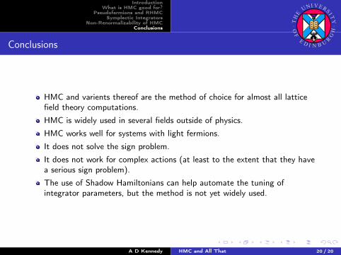
HMC and varients thereof are the method of choice for almost all latticefield theory computations.

HMC is widely used in several fields outside of physics.

HMC works well for systems with light fermions.

It does not solve the sign problem.

It does not work for complex actions (at least to the extent that they havea serious sign problem).

The use of Shadow Hamiltonians can help automate the tuning ofintegrator parameters, but the method is not yet widely used.


THE

UNIVERSI T

Y

OF

E D I N B U RGH

hmc and all that - bu blogs – blogs for the boston...

Documents