Pyramid Coding and Subband Coding

. Basic Idea: Successive lowpass filtering andsubsampling.

rip" 10.33 Processor generatingthe i + Ith.level image/'..(11.. "2) from theith.levelimage/'{II..1Iz)in Gaussianpyramidimagerepresentation.

. Filtering:

fp(nl' n2) = fi(nI, n2) * h(nI, n2)

o <nI,n2< 2M-lOtherwise

. Type of filter determines the kind of pyramid.

-- -Gaussian -pyramid: h( nl, n2} ...= h( nl)h(n2)a n=O

h(n) = ~ 1 n = :1:1

t - ~ n = ;j:2

a is between .3 and .6

109

"--.. -.... ~... ~I"'

P~ramid Coding and Subband Coding

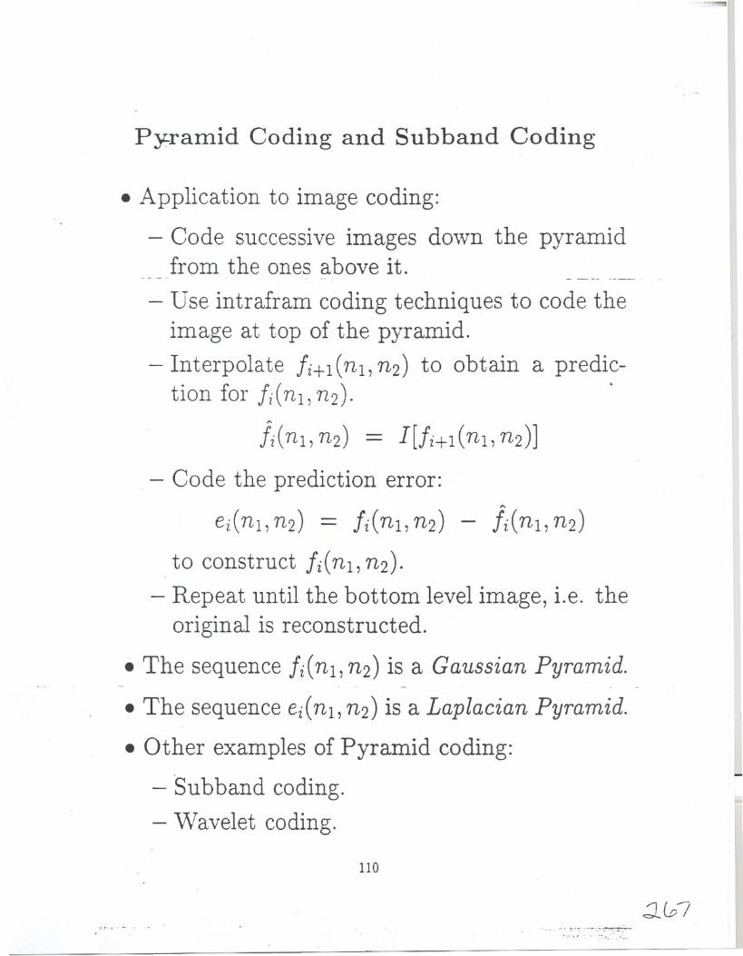
. Application to image coding:

- Code successive images do\vn the pyramidfrom the ones above it. - - -- -----

- Use intrafram coding techniques to code theimage at top of the pyramid.

- Interpolate fi+l (nl, n2) to obtain a predic-tion for fi(nl, n2)' .

Ji(nl, n2) = I[fi+l (nl, n2)]

. - Code the prediction error:

ei(nl, n2) = fi( nl, n2) - Ji(nl, n2)

to construct fi( nl, n2)'

- Repeat until the bottom level image, Le. theoriginal is reconstructed.

. The sequence !i(nl,n2) is a Gaussian Pyramid.- - -

. The sequence ei(nl, n2) is a Laplacian Pyramid.

. Other examples of Pyramid coding:

- Subband coding.- Wavelet coding.

;...

110

.~..,- _0 ::_0"":, ~~_. '1... ....

-..............

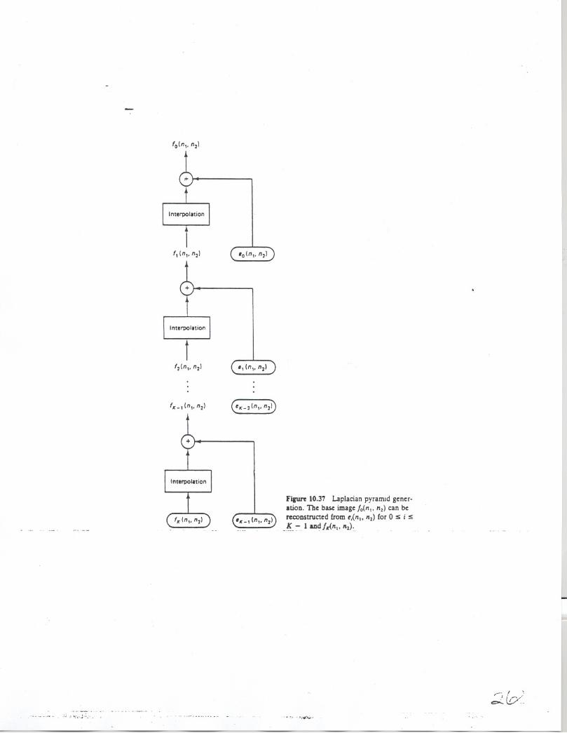
Fipn 10.37 Laplacian pyramId gener-

atioD. ibe base image /o(lIt. "2) can berecoDStructed from t,{lIto 112)for 0 s i s

_I!:_:- 1and/«<lItoIl2)'_

,_' I \-!.. b<

.., ~ .,..........

1

Figure 10.36 Exampie of the GauSSIan pyramid representation for image of 513 x 5D pixel;.wllh K = J.

The Gaussian pyramid representation can be used in developing an approachto image coding. To code the original image 1\1(111,II:). we code fl(II;. 11:)and thedifference between fur11,.11:)and a prediction of lu(IIJ. II~) from /1(11:. ":). Supposewe predict fu(1I!. 11:.1by interpolating/l(II!. II~). Denoting the interpolated Imageby f~(lli. II:). we find that the error signal t"J(IIJ. II:) coded is

eo(IlI.II:) = 10(111, II~) - l[1t(II\. II~)I (lOA6)=fo(lIl. II~) - fj(lIl. II:)

where 1[.] is the s?atial interpolation operation. The interpolation process expandsthe support size of 11(111, 11:). and the support size of fj(lIl. II:) is the same asfill,. 11:). One advantage of coding /1(111,II:) and t'o(lIl. II:) rather than 10(11,.":) isthat the coder used can be adapted to the characteristics of 11(111.11:)and eu(II!. ":1.Ii we do not quantlze 11(111.11:)and eo(lIl. II:). from (10.46) 10(111.11:)can be recovered

_ exactly by

(10..r7)

In image coding.j:(III. II:) and eo(lIl.II:) are quantized and the reconstructed imageju(II:. 11:)is obtained from (10.47) by

jo(lIl. II:) = 1[j1(1I1. 11:)] + eo(lIl. 11:) (10AS)

where .fU(III'11:)and eo(lIl. 11:)are quantized versions of fu(lIt. II:) and eo(II!. II:).If we stop here. the structure of the coding method is identical to the two-channelcoder we discussed in the previous section. The image 11(111,11:)can be viewedas the subsampled lows component fLS(lII' ":) and eo(1IJ' II:) can be viewed as thehighs component fH(II:. II:) in the system in Figure 10.31.

636 Image Coding Chap. 10

Figure 10.38 Example of the Laplacianpyramid imagerepresentationwith K = 4. Theoriginal image used is the 513 x 513-pixelimage!o(nh n:) in Figure 10.36. t,(n,. n:) [or0:5 i :5 3 and !.(n,. n:).

the difference of the two Gaussian functions. The difference of two Gaussians

can be modeled [Marr] approximately by the Laplacian of a Gaussian, hence thename "Laplacian pyramid."

From the above discussion, the pyramid coding method we discussed can beviewed as an example of subband image coding. A.s we have stated briefly, insubband image coding. an image is divided into different frequency bands and eachband is coded with its own coder. In the pyramid coding method we discussed.the bandpass filtering operation is performed implicitly and the bandpass filtersare obtained heuristically. In a typical subband image coder, the bandpass filtersare designed more theoretically [Vetterli; Woods and O'Neil].

Figure 10.39 illustrates the performance of an image coding system in whichfK(nl' n2) and e,(nl, n:) for 0 s is K-1 are coded with coders adapted to thesignal characteristics. Qualitatively, higher-level images have more variance andmore bits/pixel are assign-ed. FortUnately, however, they are smaller in size. -Fig-ure 10.39 shows an image coded at ! bitipixel. The original image used is the 513x 513-pixel image fo(nl, n2) in Figure 10.36. The bit rate of less than 1 bitipixelwas possible in this example by entropy coding and by exploiting the observationthat most pixels of the 513 x 513-pixel image eo(nl, n2) are quantized to zero.

One major advantage of the pyramid-based coding method we discussedabove is its suitability for progressive data transmission. By first s-=ndingthe top-level image fK(nl, n:) and interpolating it at the receiver, we have a very blurredimage. We then transmit eK_I(nl' n2) to reconstruct fK-I(nl, II:), which has ahigher spatial resolution than fK(nl, n2)' As we repeat the process, the recon-structed image at the receiver will have successively higher spatial resolution. Insome applications, it may be possible to stop the transmission before we fully

Sec. ,0.3 Waveform Coding 639

Figurf 10.39 Example of the laplacianp~T3mid image coding "'lth K = .Ial! bit:pixel. The ongmallmage used IS

the 513 x 513'plXellmage joIn,. n:) 10Figure 10.36.

recover the base level image fu(1I1'n~). For example. we may be able to judgefrom a blurred image that the image is not what we want. Fortunately. the imagesare transmitted from the top to the base of the pyramid. The size of imagesincreases by approximately a factor of four as we go down each level of the pyramid.

In addition to image coding. the Laplacian pyramid can also be used in otherapplications. For example. as we discussed above. the result of repetitive inter.polation of E'j(lIj.n2)such that its size is the same as that of fu(II!. II~)can be viewedas approximately the result of filtering fo(nj. n2) with the Laplacian of a Gaussian.As we discussed in Section 8.3.3. zero-crossing points of the result of filtering/0(11).n2) with the Laplacian of a Gaussian are the edge points in the edge detectionmethod by Marr and Hildreth.

10.3.6 Adaptive Coding and Vector Quantization

The waveform coding techniques discussed in previous sections can be modifiedto adapt to changing local image characteristics. In a PCM. system. !he_re~o_n~.struction levels can be chosen adaptively. In a DM system. the step size .1 canbe chosen adaptively. In regions where the intensity varies slowly. for example.A can be chosen to be small to reduce granular noise. In regions where the intensityincreases or decreases rapidly. .:1can be chosen to be large to reduce the slopeoverload distonion problem. In a DPCM system. the prediction coefficients am.!the reconstruction levels can be chosen adaptively. Reconstruction levels can alsobe chosen adaptively in a two-channel coder and a pyramid coder. The numberof bits assigned to each pixel can also be chosen adaptively in all the waveformcoders we discussed. In regions where the quantized signal varies very slowly. forexample. we may want to assign a smaller number of bits/pixel. It is also possibleto have a fixed number of bits/frame. while the bit rate varies at a pixel level.

In adaptive coding. the parameters in the coder are adapted based on some

640 Image Coding Chap. 10

.:;17i

.-'-"1.

I

I

I

IIIIiIii

Subband Coding

. . . . t 2X(n)

. . . . t 2

A 1

X(ro) = 2 [Ho(ro)Go(ro) + H1(ro)G1(ro)]X(ro) +

~ [Ho( ro + i)Go( ro) + HI (ro + n)G1 (ro) ]X( ro + n)

Consider QMF Filters:

Ho(ro) = Go(-OO) = F(ro)

jroHI ( ro) = G 1(-(0) = e F( - ro + 1[)

A 1 ~/

~ X(ro) = 2 [F(ro)F(-ro)+ F(-ro+n)F(ro+n)]/f'0

2 2IMPOSE: IF(oo)1 +IF(ro+1[)1 = 2

~ X(ro) = X(oo) ~ Perfect Reconstruction

Filter Design:

l..

i.I

· QMF filters:

N = # of taps

· Johnston's filter coefficients

ho(N - 1 - n) = ho(n)

~ symetric ~ NPR

8 tap Johnston filters:

h (0) = h (7) = 0.00938

h (1) = h (6) = 0.06942

h (2) = h (5) = -0.07065

h (3) = h (4) = 0.489980L..

Filter Design

· Cannot have linear phase FIR filters

for QMF condition except for trivial

2 tQP filter

~ amplitude distortion

· Well known filters

Ho(ro) = A(ro) Go(ro) = B(ro)

H1(ro) = ej())B(ro+1t)

G1(ro) = e-j())A(ro+1t)

a(n) = [1,2,1]

hen) = [-1,2,6,2,-1]

~ simple to implement

proposed by LeGa11

Filter Design:

* Smith and Barnwell

h(O) = 0.03489

h(l) = -0.0109

h(2) = -0.0628

h(3) = 0.2239

h(4) = 0.55685

h(5) = 0.35797

h(6) = -0.0239

h(7) = -0.0759

)

Bit Allocation in Subband Codin

R = Average # of bits per sample

RK = Average # of bits per sample of subband K

M = # of subbands

variance of coefficients in subband K:

)

...

2D Subband Coding

· Separable > Easy to implement

. Nonseparable

SeDarable subband Coding:

HaY

H1y

o

)Analysis

FREOUENCY DOMAIN

')lD

-1t

2D

highpass

roLowpass +1t

)

11\

T

I I

4I

2 2I

4I I1 I

. I 1----------- ------------I 1

I I

3 I1 1

1 3I 1I I

II

-1t'T I

I 1 +1tI I

3 I 1 1 I 31 II 1

-----T----- ------1-----1 I

4I

2 21

4I II I

-1t

Wavelets

') · A special kind of Subband Transform

· Historically developed independent ofsubband coding

K(n)

...

. . .

/Ho

DesspecbeWDec

o II ro

-Ho

-Ho I- t2 -

-Ho

- t 2H- I

HI- t 2....

-HI t2

X(ro)

0

t;ition

4 3 2 1j,..

-

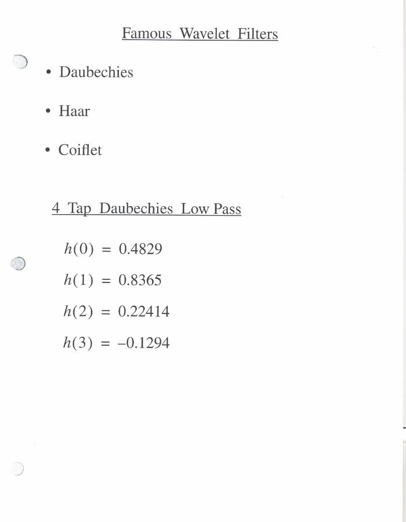
Famous Wavelet Filters

'9. · Daubechies

· Haar

· Coiflet

4 TaD Daubechies Low Pass

h(O) = 0.48291'.

'3.r.J

\;<'. '''';""I,::~,

h( 1) = 0.8365

h(2) = 0.22414

h(3) = -0.1294

j

)

Fractal Compression

· Founders: Manderblothand Bamsley.

· Basic idea: fixed point transformation

· Xo is fixed point of function f if

f(Xo) = Xo

· Example: Transformation ax + b

has a fixed point Xo given by:

Xo = aXo + b

· To transmit Xo' send a, b

Then iterate:

X (n+ 1) - X (n) bo - a 0 +

will converge regardless of initialguess.

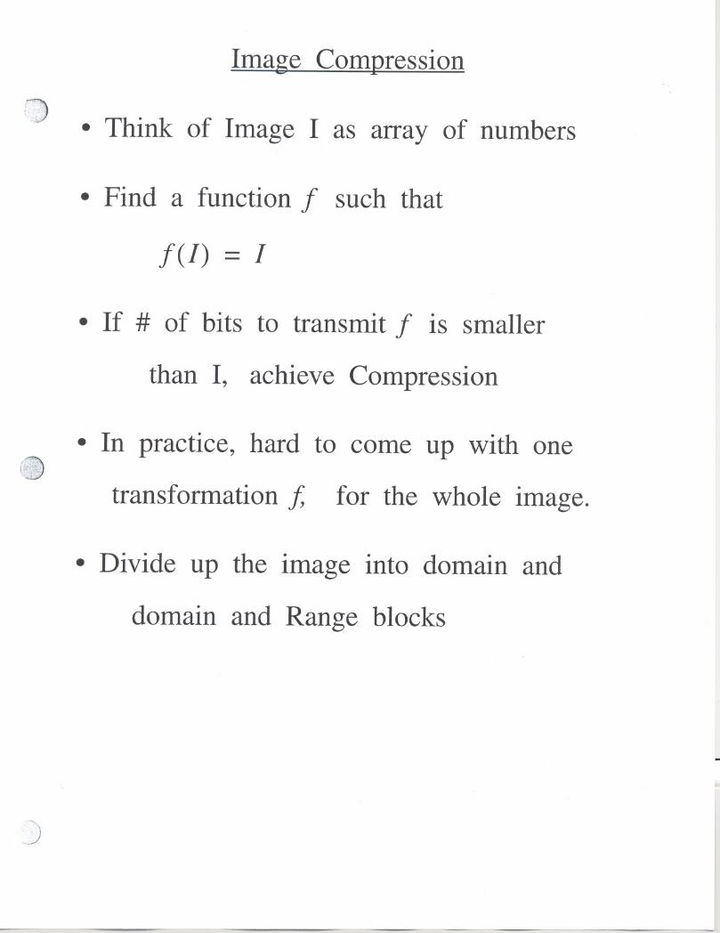
Image Compression

· Think of Image I as array of numbers

· Find a function I such that

1(1) = I

· If # of bits to transmit I is smaller

than I, achieve Compression

· In practice, hard to come up with one

transformation f, for the whole image.

· Divide up the image into domain and

domain and Range blocks

)

Image Compression

· Main idea:

- Divide up image into M x M"Range" blocks

- For each Range block findanother 2 M x 2 M

"Domain block" from

the same image such that for some

transformation f K we

get f K(DK) = RK

D K = Domain block k

R K = Range block k

· First publicly discussed byJacquin in 1989 thesis + 1992paper

· Works well if there is self

similarity in image.)

Range Domain

---1 I.I I I I

-+--t-+-+I I I I

· What should f K do?

'

I)'( ..<

change size of domain blockchange orientation of domain blockchange intensity of pixels

· f K consists of

geometric transformation : gK

massic transformation : m K

displacement + size + it' te,,~ ;+y

orientation+~

Transformations:

· gK : displaces + adjusts intensity

~ easy

i can be

* Rotation by 90, 180, -90* Reflection about

horizontal, vertical, diagonal:.) * identity map

· Finding transformations iscompute intensive

· Search through all domainblocks + all transformations tofind "BEST" one

· Encoding more time than decoding

· If Image is divided mtD

N Range blocks ~ N

transformations IK k=l,...N

are its representation.

1 = 1(1)

A

I is approximation to I.

· Collage theorem guarantees convergence

A

to I using any arbitrary initial

guess for image.

)

378 1 3 ANALYSIS/SYNTHESIS SCHEMES 13.5 Sur

FIGU I

The

ity of treCQJ1S1relativchas onlin appltimes.

13.

Weha'

codinggeneraconstncationwanttlvide h:to be ~G.728FIGURE 13.11 The fint six Iterations of the fractal decoding process.

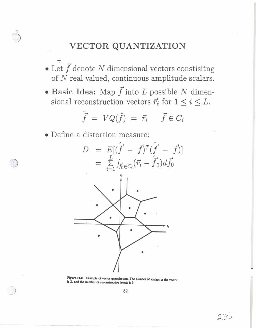
VECTOR QUANTIZATION- -

. Let f denote N dimensional vectors constisitngof N real valued, continuous amplitude scalars.-

. Basic Idea: Map f into L possible N dimen-sional reconstruction vectors fi for 1 < i < L.

,.,

f = VQ(j) = fi

. Define a distortion measure:

f/Ipft .1.' Eumpfe 01-=tor quaalizalioa.TbeDlUDberollCllara iDthe Wdoris 2, Uld the DlUDberof recDaIIl1IcIioaIeYCbis 9.

82

properties of Vector Quantization

. Removes linear dependency between randomvariables.

. Removes nonlinear dependency between ran-dom variables.

. ExpJits increase in dimensionality.

. Allo1vsus to code a scalar with less than onebit.

) . Computational and storage requirements arefar greater .than scalar quantization.

)83

VQ RemovesLinear Dependency-. Linear transformation can decorrelate linearly

dependent (correlated) random variables.

.

J

1.1

.

F1pn 11.J0 Result or clillliJulin& lineu

dependence or lbe IWOsalin I. IDd IJill F"Jlurc 10.9 by IiDcar trutslonnalioaof I, 8Dd 11'

~37

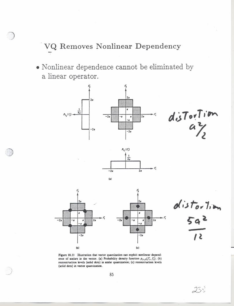
)-VQ RemovesNonlinear Dependency

. Nonlinear dependence cannot be eliminated by

a linear operator.

'i

Ib)

F"1III1"t10.11 JUustration that vector quantization can exploit _linear depend-ence of lCI.Ian in the vector. (a) Probability density function P,'n(f;. Ii); (b)realnstruction levels (lOIid dou) in scalar quantization; (c) rec:oostnaction levels(solid dou) in vector quantizatioa.

) 85

VQ ~xploits the Increase in Dimensionality

. The mean square error due to VQ is approxi-mately less than 4 percent than scalar quanti-zation. bn 1k ~~ -:# ~ r,e.~ :s~t:,." 1>4~is;

)

lal

...

Ibl

j86

..

. .. .. .. . . .... .... . . .. . . .... .... . . .. .. .. .

Codebook Design Algorithms-. I{-means algorithm.

. Tree codebooks and binary search.

. Nearest neighbor.

{~~;.~

87

1.' 1'- ,cx-r..-/

Codebook Design via K-means-

. Exploit the following two necessary conditionsfor the optimal solution:

-.- For a vector f to be quantized to one of

the reconstruction levels, the optimal quan-tizer must choose the reconstruction level 'Pi-.

V\Thich has the samllest distortion between f.-. · -.', . 'i' .J {' \' t . \, / J / t '\

an d r i. rj ~ ~:: -(: 1+-0. (-t ) '( , ) '. C' I ""1 ~ -( ') )

- Each reconstruction level fi must minimizethe average distortion D in Ci.

-. -.lYlinimize E(d(f, 'Pi) I fECi] W.T.t. 'Pi

. Find Ti and Ci iteratively ~ Problem: localversus global minimum ~ initial guess impor-t ant IMlat CDd8book 1IICt0l1. ~1SISL

JCl8aification of M hl"i"" 1IICt0l1to L ~ by qllMtiution

1

Estimation of " by computingCllntrold 0' the 1IICt0l1 withinIKtt duster

J

\ .r.,\ / 1 ,

. -) -.. ~

") ~j

r"),1 I :

~~(

- Complexity of K-means

. M training vectors, L codewords, N dimensional,R bits per scalar.

. Complexity of Codebook design:

- M L evaluation of distortion measure for each

L;- 11 'rZ/ ;?> iteration.

. - 1\1LN = N M2-NR additions and mults per'iteration.

- Example: N= 10, R=2 , M = 10L results in100 trillion operation per iteration.

- Storage: MN for training vectors, LN for re-construction levels ~ (M + 2~R)N. ~> .. -,

. ", I :

. Complexity of operation at the receiv~.-r\(~ '. e.-. ;1 ' I

I -. /~ 1,/ 9

- Storage of reconstruction levels: N2N R." IfN = 10 and R = 2, storage is 10 million.

- Number of artithemetic operations N2NR:'IfN = 10 and R = 2, 10 million operations perlook up.

89

)

Tree Codebook and Binary Search

J

. Full search is responsible for exponential growthof the number of operations at the r0@Qi~.~~r-+Tree codebook. T~~tt., ·

. Let L be a power of 2.

. Basic operation of tree codebook design:

- Use K-means to divide the N dimensional....

space of f into t\VOregions.

- Divide each of the two regions into two moreregions using the K-means algorithm.

- Repeat step 2 until there are L reconstruc-tion levels.

I'Jpre .U5 Eumple or . Ireeaide.'M boot.'r '.

)90

)

JA.:: :f1 if 7~ uWO~J

t,~* ".,~()

. .

fJ = ,~vS. ~

Complexity of Tree Codepook... ._ ..J- .. T"'"'( ...... ~ f ..; ...1 , ' , :...c _r :..,...., .' r.'" . t r /'" ~y-'..,-. _ '.." ~'J '"'"-:\ I c. - ';",

D .1 /. ./-/ o-! s1 ~~~. eSlgn comp ~Xlty: r 'G .-~

- Numbf;Lof arlth~~ operations per itera-tion is.2N A( log2L,j For N = 10 and R = 2,the reductioilIactor compared to the fullsearch is 26, 000.

- Storage: approximat;~ly. the same as full,s~arch1

.th 1 -, : . ,,' 7 ,...1._ ,_ -I. )a gorl m. '~i cY1'~ ! (M F" ~ 7~~ .'.' .-' .. r.'L,.:."

. Operation complexity at r€cciverT(c~/"

- Number of arithmetic operations Is 2N2R. :; 2 ~ I~~) LFor N = 10 and R = 2, the reduction factorcompared to the full search is 26, 000.

- Storage: The codebook must store all theintermediate reconstruction levels as well asthe final reconstruction levels. ~ Twice asmuch storage needed as full search.

. Distortion of full search is slightly smaller thanthat of tree search.

)

)91

liearest Neighbor Design Algorithm

. Initially proposed by Equitz.

. computational complexity grows linearly withthe training set.

. Find the 2 vectors closest to each other, mergethem into another vector equal to their mean,repeat this process until the number of vectors!is L.

. I\1ain efficiency is achieved by partitioning the<:) training d8:tainto a K-D tree ~ multiple merges

at each iteration.

92

I'-u.L .- /

- Variations of VQ

. Multistage VQ reduces storage and search time.

1. First stage a low rate VQ.2. Generate error by subtracting the codeword

from the original.3. Code the error by a different VQ.

4. Repeat steps 2 and 3.

/~';J/

TO CHANNEL

. \

INDEx 2INOEXI

Fia. 5.5.2 Multistaae Vcaor Quantizatioa. At each ltate an error YCCtoris computed.which is then used u the input 10the DCxt.tale or VQ. The decoder merelycomputes. lummatiOllor the code YCCtOncorrespoaclinllO the receivedindica.

. Parameter extraction techniques:

- mean and variance of each input vector arecomputed and sent separately.

- mean and variance might be coded with DPCM.

) 93

Variations of VQ (cont'd)-. Block classification:

- Divide the blocks into several classes accord-ing to spatial activity.

- Design a codebookfor each class.- Overhead on transmitting the codebook is

large.

. Combine prediction techniques with VQ:

- Coded quantity is the prediction error ratherthan int~nsity values.

. \TQ of color images exploits the correlation be-t\veen color components.

. Typical rates: .1 to .5 bits per pixel for 4 x 4pixels as vectors.

J 94

/-1:,.-...r.-- \

rI

local measure. such as local image contrast. If the local measure used can beobtained from previously coded pixel intensities. then it does not have to be trans-mitted. If the local measure used is obtained directly from [(nt. n;:). it must betransmitted. since the receiver does not have access to the original image. Adaptivecoding cenainly adds complexity to an image coder. but can often significantlyimprove its performance.

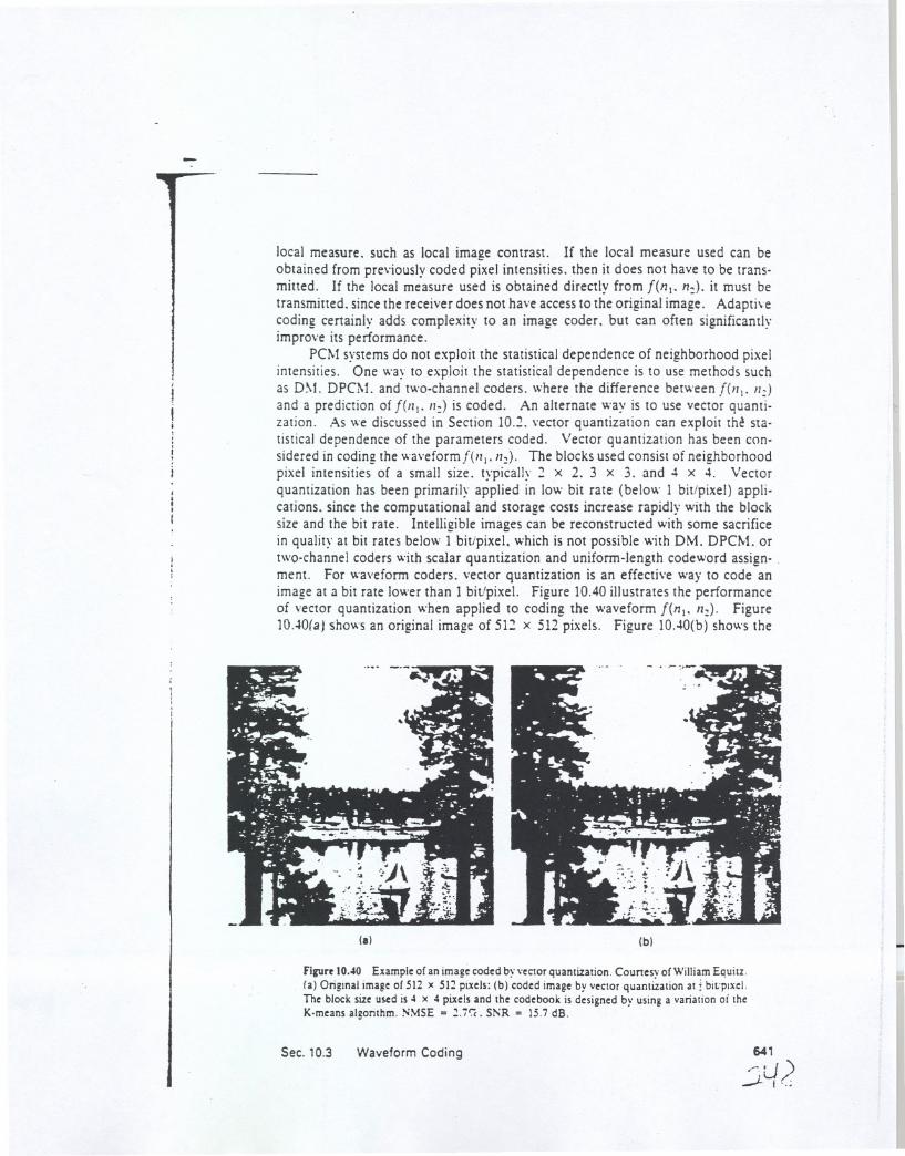
PCM systems do not exploit the statistical dependence of neighborhood pixelintensities. One way to exploit the statistical dependence is to use methods suchas D~L DPCM. and two-channel coders. where the difference between f(1ll. ":)and a prediction of [(III' II:) is coded. An alternate way is to use vector quanti-zation. As we discussed in Section 10.2. vector quantization can exploit th~ sta-tistical dependence of the parameters coded. Vector quantization has been con-sidered in coding the wa\'eform[(III.II~). The blocks used consist of neighborhoodpixel intensities of a small size. typically ~ x 2. 3 x 3. and ~ x 4. Vectorquantization has been primarily applied in low bit rate (below 1 bit/pixel) appli-cations. since the computational and storage costs increase rapidly with the blocksize and the bit rate. Intelligible images can be reconstructed with some sacrificein quality at bit rates below 1 bit/pixel. which is not possible with DM. DPCM. ortwo-channel coders with scalar quantization and uniform-length codeword assign- .

ment. For waveform coders. vector quantization is an effective way to code animage at a bit rate lower than 1bit/pixel. Figure 10.40illustrates the performanceof vector quantization when applied to coding the waveform [(nt. II~). Figure10.~0(a' shows an original image of 51:! x 512 pixels. Figure IOAO(b)shows the

lei Ibl

Flgurt 10.40 Example of an image coded by vector quantization. Counesy of William Equitz.

la) Original image or 512 x 51:! pixels: (b) coded image by vector quantization at i biliplxel.The block size used is 4 x 4 pixels and the codebook is designed by using a variation oi theK.means algorithm. NMSE .. :!.i':C. SI'R .. 15.7 dB.

Sec. 10.3 Waveform Coding 641

r.U ).-L I".;

L