holography for cosmology - kavli institute for the physics ... · holography for cosmology kostas...

IntroductionPart I: Holographic dictionary

Part II: New holographic modelsConclusions

Holographyfor Cosmology

Kostas SkenderisInstitute for Theoretical PhysicsGravitation and AstroParticle PhysicsAmsterdam (GRAPPA)KdV Institute for MathematicsUniversity of Amsterdam

Kostas Skenderis Holographic Non-Gaussianity



GRAPPA

A new initiative formed by three physics institutes:

Institute for Theoretical Physics (ITFA)Affiliate members: J. de Boer, E. Verlinde, K. Skenderis, M.Taylor, P. van der SchaarInstitute for High Energy Physics (IHEF)Affiliate members: S. Bentvelsen, E. de Wolf, E. Laenen, P.Kooijman, P. de JongAnton Pannekoek Institute (API) for astronomyAffiliate members: R. Wijers, A. Watts, M. van der Klis, S.Markoff, R. Wijnands

We are currently searching for at least four new facultymembers in senior and junior ranks, tenured ortenure-track.




Outline

1 Introduction

2 Part I: Holographic dictionaryCosmological PerturbationsThe domain-wall/cosmology correspondenceHolography: a primerCorrelators for holographic RG flowsHolography for cosmology

3 Part II: New holographic models

4 Conclusions




Introduction

Over the last two decades, striking new observations havetransformed cosmology from a qualitative to a quantitative science.




COBE (1989)




WMAP (2001)




Planck (2009)




Primordial perturbations

The primordial perturbations offer some of our best clues as to thefundamental physics underlying the big bang. Their form appears tobe very simple:

Small amplitude: δT/T ∼ 10−5.Nearly Gaussian.Nearly scale-invariant.Adiabatic.

Any proposed cosmological model must be able to account for thesebasic features, and any predicted deviations (e.g. from Gaussianity)are likely to prove critical in distinguishing different models.




The primordial power spectrum

A Gaussian distribution is fully characterised by its 2-point function orpower spectrum. From observations, the power spectrum takes theform:

∆2S(q) = ∆2

S(q0) (q/q0)nS(q)−1

The WMAP data yield (for q0 = 0.002Mpc−1)

∆2S(q0) = (2.445± 0.096)× 10−9, nS−1 = −0.040± 0.013,

i.e., the scalar perturbations have small amplitude and are nearlyscale invariant.

These two small numbers should appear naturally in any theorythat explains the data.




Non-Gaussianity

Non-Gaussianity implies non-zero higher-point correlation functions.The lowest order is the 3-point function, or bispectrum, of curvatureperturbations ζ:

〈ζ(q1)ζ(q2)ζ(q3)〉 = (2π)3δ(∑

qi)B(qi)

Non-Gaussianity arises from nonlinearities in cosmological evolution.The three main sources are:

1. Nonlinearities (interactions) in inflationary dynamics.2. Nonlinear evolution of perturbations in radiation/matter era.3. Nonlinearities in relationship between metric perturbations and

CMB temperature fluctuations. (To linear order, ∆T/T = (1/3)Φ).




Non-Gaussianity

Non-Gaussianity is important as it potentially provides a verystrong test of inflationary models. The amplitude of thebispectrum is parametrised by fNL:

B(qi) = fNL × (shape function)

Different inflationary models give different predictions for fNL andshape function.




The shape of non-Gaussianity

Local form [Gangui etal (1994)]; [Verde etal(2000)] ; Komatsu &Spergel (2001)]

Blocal(q1, q2, q3) = f localNL

6A2

5q31q3

2q33

3∑i=1

q3i , A = 2π2∆2

S(q)

→ WMAP7: f localNL = 32± 21(68%CL)

→ Single scalar slow-roll inflation: f localNL ∼ O(ε, η) ∼ 0.01

Equilateral form [Creminelli etal, astro-ph/0509029]]

Bequil(q1, q2, q3) = f equilNL

18A2

5q31q3

2q33

(−2q1q2q3 −

3∑i=1

q3i + (q1q2

2 + 5 perm)

)

→ WMAP7: f equilNL = 26± 140(68%CL)

The Planck data (expected next year) should be sensitive to just

fNL ∼ 5.




Holographic Universe

In this talk I will present new holographic models for the very earlyuniverse:

In these models, the very early universe is non-geometric andhas a weakly coupled description in terms of a three dimensionalQFT.They provide a new mechanism for a scale invariant spectrum.They are compatible with current observations, yet they havedifferent phenomenology than conventional inflation.




References

The talk is based onwork with Paul McFaddenHolography for Cosmology, arXiv:0907.5542The Holographic Universe, arXiv:1007.2007Observational signatures of holographic models of inflation,arXiv:1010.0244Holographic Non-Gaussianity, arXiv:1010.????on-going work with Adam Bzowski and Paul McFadden




Holography for cosmology

Any holographic proposal for cosmology should specify

1 what the dual QFT is2 how it can be used to compute cosmological observables (the

holographic dictionary)

Having defined the duality,

the new description should recover established results in theregime where the weakly coupled gravitational description is validnew results should follow by using the duality in the regimewhere gravity is strongly coupled.




Main results

Our two main results are:

Standard inflation is holographic.

There are holographic models that have different phenomenology thanslow-roll inflation but they are nevertheless consistent with current ob-servations. The Planck data has the power to comfortably refute orconfirm these models.




Plan

In the first part, I will explain the sense in which inflation isholographic.

Review standard inflationary computations.Review how to compute strong coupling QFT results usingstandard gauge/gravity duality.Show that the inflationary results can be fully expressed in termsof correlators of strongly coupled QFTs.

In the second part, I will discuss the new holographic models. Whilestandard inflation is linked to strongly coupled QFTs, the new modelsare based on weakly coupled three dimensional QFT.




Cosmological PerturbationsThe domain-wall/cosmology correspondenceHolography: a primerCorrelators for holographic RG flowsHolography for cosmology

Outline

1 Introduction



4 Conclusions





Cosmological Perturbations

We start by reviewing standard inflationary cosmology.

We will discuss (for simplicity) single field four dimensionalinflationary models,

S =1

2κ2

∫d4x√−g(R− (∂Φ)2 − 2κ2V(Φ))

We assume a spatially flat background (for simplicity)

ds2 = −dt2 + a2(t)dxidxi

Φ = ϕ(t)

The physical degrees of freedom are a scalar field ζ and atransverse traceless metric γij.





Power spectrumIn the inflationary paradigm, cosmological perturbations are assumedto originate at sub-horizon scales as quantum fluctuations.

Quantising the perturbations in the usual manner,

〈ζ(t,~q)ζ(t,−~q)〉 = |ζq(t)|2

〈γij(t,~q)γkl(t,−~q)〉 = 2|γq(t)|2Πijkl,

where Πijkl is the transverse traceless projection operator andζq(t) and γq(t) are the mode functions.The superhorizon power spectra are obtained by

∆2S(q) =

q3

2π2 |ζq(0)|2, ∆2T(q) =

2q3

π2 |γq(0)|2,

where γq(0) and ζq(0) are the constant late-time values of thecosmological mode functions.





Non-gaussianity

Non-Gaussianity is related to higher-point functions. In this talkwe focus on the three-point function of ζ. This is computed usingthe in-in formalism as

〈ζ3(t)〉 = −i∫ t

t0dt′〈[ζ3(t),Hint(t′)]〉

where Hint is obtained by expanding the action to cubic order.This leads to

〈ζq1ζq2ζq3〉 = (2π)3δ(q1 + q2 + q3)B(q1, q2, q3)

Different models are characterized by different B(q1, q2, q3).





Response functions

Let us now reformulate these results in terms of response functions.

The response functions, Ω2,Ω3,E2, . . ., are defined by

Π(~x1) =∫

d3x2Ω2(~x1 −~x2)ζ(~x2)+∫

d3x2d3x3Ω3(~x2 −~x1,~x3 −~x1)ζ(~x2)ζ(~x2)+· · · ,

Πγij (~x1) =

∫d3x2E2(~x1 −~x2)γij(~x2) + · · · ,

where Π and Πγij are the canonical momenta of ζ and γij and the dots

indicate other terms that are quadratic and higher order influctuations.





Perturbation equations

The field equations can be written in terms of response functions andwe present here the ones associated with ζ:

0 = Ω2(q) +1

2a3εΩ2

2(q)− 2aεq2,

0 = Ω3(qi) +1

2a3ε

(Ω2(q1) + Ω2(q2) + Ω2(q3)

)Ω3(qi) + X (qi),

where X (qi) depends on the interactions, ε = 2(H′/H)2 and H is theHubble function.





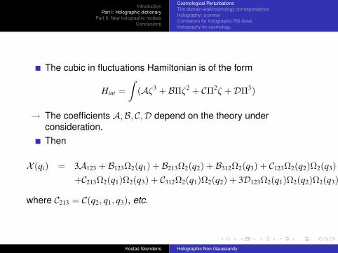
The cubic in fluctuations Hamiltonian is of the form

Hint =∫

(Aζ3 + BΠζ2 + CΠ2ζ +DΠ3)

→ The coefficients A,B, C,D depend on the theory underconsideration.Then

X (qi) = 3A123 + B123Ω2(q1) + B213Ω2(q2) + B312Ω2(q3) + C123Ω2(q2)Ω2(q3)+C213Ω2(q1)Ω2(q3) + C312Ω2(q1)Ω2(q2) + 3D123Ω2(q1)Ω2(q2)Ω2(q3)

where C213 = C(q2, q1, q3), etc.





Solution

The equations for the response functions can be solved:Ω2(q) = 2a3εζq/ζq

Ω3(z, qi) = −(∏

i 1/ζqi(z)) ∫ z

z0dz′X (z′, qi)

∏i ζqi(z

′),where ζq is a solution of the linearised equation of motion

0 = ζq + (3H + ε/ε)ζq − a−2q2ζq,





Response functions and 2- and 3-point functions

One can show that

|ζq|−2 = −2Im[Ω2(q)], |γq|−2 = −4Im[E2(q)].

so the power spectra can be expressed in terms of the late timebehavior of the response functions.One can also show that

B(q1, q2, q3) ∼Im[Ω3(q1, q2, q3)]∏3

i=1 Im[Ω2(qi)]

evaluated at late times.

We will next show that Ω2(q), E2(q) and Ω3(q1, q2, q3) are related totwo- and three-point functions of a strongly coupled 3d QFT.





Outline

1 Introduction



4 Conclusions





Domain-wall/cosmology correspondence

The springboard for our discussion is a correspondence betweencosmologies and domain-wall spacetimes.

Domain-wall spacetime:

ds2 = dr2 + e2A(r)dxidxi

Φ = Φ(r)

This solves the field equations that follow from

SDW =1

2κ2

∫d4x√

g [−R + (∂Φ)2 + 2κ2V(Φ)],






One can prove the following:

Domain-wall/Cosmology correspondence

For every domain-wall solution of a model with potential V there is aFRW solution for a model with potential (V = −V). [Cvetic, Soleng(1994)], [KS, Townsend (2006)]

The correspondence can be understood as analytic continuation.The flip in the sign of V guarantees that the metric remains real.An equivalent way to state the correspondence is

κ2 = −κ2





Domain-walls and holography

Domain-wall spacetimes enter prominently in holography. Theydescribe holographic RG flows.

The AdSd+1 metric is the unique metric whose isometry group isthe same as the conformal group in d dimensions. This is themain reason why the bulk dual of a CFT is AdS.The domain-wall spacetimes are the most general solutionswhose isometry group is the Poincaré group in d dimensions.Thus, if a QFT has a holographic dual the bulk solution must beof the domain-wall type.





Holographic RG flows

There are two different types of domain-wall spacetimes whoseholographic interpretation is fully understood.

1 The domain-wall is asymptotically AdSd+1,

A(r) → r, Φ(r) → 0, as r →∞

This corresponds to a QFT that in the UV approaches a fixedpoint. The fixed point is the CFT which is dual to the AdSspacetime approached as r →∞.





Holographic RG flows

2 The domain-wall has the following asymptotics

A(r) → n log r, Φ(r) →√

2n log r, as r →∞

This case has only been understood recently [Kanitscheider, KS,Taylor (2008)] [Kanitscheider, KS (2009)].

→ Specific cases of such spacetimes are ones obtained by takingthe near-horizon limit of the non-conformal branes (D0, D1, F1,D2, D4).

→ These solutions describe QFTs with a "generalized conformalstructure": all terms in the action have the same scaling andthere is a dimensionful coupling constant.






Let us see how the correspondence acts on the domain-wallsdescribing holographic RG flows.

1 Asymptotically AdS domain-walls are mapped to inflationarycosmologies that approach de Sitter spacetime at late times,

ds2 → ds2 = −dt2 + e2tdxidxi, as t →∞

2 The second type of domain-walls is mapped to solutions thatapproach power-law scaling solutions at late times,

ds2 → ds2 = −dt2 + t2ndxidxi, as t →∞





Outline

1 Introduction



4 Conclusions





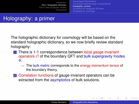
Holography: a primer

The holographic dictionary for cosmology will be based on thestandard holographic dictionary, so we now briefly review standardholography:

1 There is 1-1 correspondence between local gauge invariantoperators O of the boundary QFT and bulk supergravity modesΦ.→ The bulk metric corresponds to the energy momentum tensor of

the boundary theory.

2 Correlation functions of gauge invariant operators can beextracted from the asymptotics of bulk solutions.





Asymptotic solutions

The standard gauge/gravity duality is based on spacetimes thatare asymptotically locally Anti-de Sitter.These spacetimes have a conformal boundary and near theconformal boundary Einstein equations (with negativecosmological constant) hold.This implies that the metric has the following asymptotic form (in4 bulk dimensions) [Fefferman, Graham (1985)]

ds2 = dr2 + e2rgij(x, r)dxidxj

gij(x, r) = g(0)ij(x) + e−2rg(2)ij(x) + e−3rg(3)ij(x) + ...

g(0)(x) is the metric of the spacetime where the boundary theorylives and (as such) it is also the source of the boundary energymomentum tensor.





Correlation functions

Using the formalism of holographic renormalization, we then finda precise relation between correlation functions and asymptotics[de Haro, Solodukhin, KS (2000)]

〈Tij〉 =3

2κ2 g(3)ij.

This formula only requires that Einstein equations hold near theconformal boundary. In particular, it is also valid when curvaturesare large in the interior.Higher-point functions are obtained by differentiating the 1-pointfunctions w.r.t. sources and then setting the sources to theirbackground value

〈Ti1j1(x1)Ti2j2(x2) · · ·Tinjn(xn)〉 ∼δ(n−1)g(3)i1j1(x1)

δg(0)i2j2(x2) · · · δg(0)injn(xn)

∣∣∣g(0)=η





Correlation functions

Thus to solve the theory we need to know g(3) as a function of g(0).This can be obtained perturbatively.

→ From gravity to QFT2-point functions are obtained by solving linearized fluctuations,3-point functions by solving quadratic fluctuations etc. Here it iscrucial that the gravitational approximation is valid and thisresults in correlators of strongly coupled QFT.

→ From QFT to gravityGiven QFT correlators one obtains an asymptotic solution. If theQFT correlators are that of weakly coupled QFT then the bulkdescription has the prescribed asymptotic behavior and isstrongly coupled in the interior.





Outline

1 Introduction



4 Conclusions





Correlation functions for holographic RG flows

To compute correlation functions we perturb around thedomain-wall. The linearized equations are given by [Bianchi,Freedman, KS (2001)], [Papadimitriou, KS (2004)],

0 = ζ + (3H + ε/ε)ζ−q2e−2Aζ

0 = γij + 3Hγij−q2e−2Aγij,

Comparing with the cosmological perturbations, we find that theequations are mapped to each other provided

q = −iq

The same holds to all order: the fluctuation equations aremapped to each other provided the momenta are continued asabove.





Correlation functions for holographic RG flows

We now want to extract 2- and 3-point functions.

Schematically, we must expand the perturbed solution nearr →∞ and extract the piece that scales like e−3r.

The part linear in fluctuation gives the 2-point function.The part quadratic in fluctuation gives the 3-point function.

It is convenient to work in terms of response functions[Papadimitriou, KS (2004)]

Π = −Ω2ζ − Ω3ζ2 + · · · , Πγ

ij = −E2γij + · · · ,

where Π, Πγij are radial canonical momenta.





2-point functions for holographic RG flows

The 2-point function of the energy momentum tensor is then given by

〈Tij(q)Tkl(−q)〉 = A(q)Πijkl + B(q)πijπkl,

where Πijkl = 12 (πikπlj + πilπkj − πijπkl), πij = δij − qiqj/q2.

A(q) = 4 [E2(q)](0) , B(q) =14[Ω2(q)

](0) .

The subscript indicates that one should pick the term with appropriatescaling in the asymptotic expansion.





3-point functions for holographic RG flows

Similarly, one can derive a holographic formula for the 3-pointfunction

〈Ti1j1(q1)Ti2j2(q2)Ti3j3(q3)〉 = ...

in terms of response functions.The 3-point function for the trace of stress energy tensor, T = T i

i ,is related to the response function Ω3 by

[Ω3(q1, q2, q3)](0) ∼ 〈T(q1)T(q2)T(q3)〉+∑

i

〈T(qi)T(−qi)〉

− 2[〈T(q1)Υ(q2, q3))〉+ 〈T(q2)Υ(q1, q3))〉+ 〈T(q3)Υ(q1, q2))〉

].

whereΥ(~x1,~x2) =

δTij(~x1)δgkl(~x2)

∣∣∣0δijδkl.





Outline

1 Introduction



4 Conclusions





Holography for cosmologyWe are now ready to present the holographic dictionary forcosmology.

The DW/cosmology correspondence maps the near boundaryregion to the late time region.Under the analytic continuation

κ2 = −κ2, q = −iq

the response functions continue as follows

Ω2(q) = Ω2(−iq), E2(q) = E2(−iq),Ω3(q1, q2, q3) = Ω3(−iq1,−iq2,−iq3).

The analytic continuations translate in QFT language to

N → −iN, q → −iq





Holographic dictionary: Power spectrum

We have shown earlier that

∆2S(q) =

−q3

4π2ImΩ(0)(q), ∆2

T(q) =−q3

2π2ImE(0)(q),

It follows

∆2S(q) =

q3

2π2

(−1

8ImB(−iq)

), ∆2

T(q) =2q3

π2

(−1

ImA(−iq)

),

where the holographic 2-point function is

〈Tij(q)Tkl(−q)〉 = A(q)Πijkl + B(q)πijπkl,





Holographic dictionary: Non-Gaussianity

We have seen earlier that

〈ζq1ζq2ζq3〉 = (2π)3δ(q1 + q2 + q3)B(q1, q2, q3)

and B(q1, q2, q3) ∼ Im[Ω3(q1, q2, q3)]/∏3

i=1 Im[Ω2(qi)].It follows

B(q1, q2, q3) = −14

1∏i Im〈T(qi)T(−qi)〉

· Im[〈T(q1)T(q2)T(q3)〉

+∑

i

〈T(qi)T(−qi)〉 − 2(〈T(q1)Υ(q2, q3)〉+cyclic perms

)],

where the imaginary part is taken after the analytic continuation.





Summary




Outline

1 Introduction



4 Conclusions




New holographic models

We are now going to obtain new models by using weakly coupledQFT. This correspond to the gravitational theory being stronglycoupled at early times.The boundary theory will be a combination of gauge fields,fermions and scalars and it should admit a large N expansion.To extract predictions we need to compute n-point functions ofthe stress energy tensor analytically continue the result andinsert them in the holographic formulae.




The holographic model

As a model one can consider the strong coupling version ofasymptotically dS cosmologies and power-law cosmology.In this work we focus on QFTs dual to the latter. These aresuper-renormalizable QFTs that depend on a single dimensionfulcoupling:

S =1

g2YM

∫d3xtr

[12

FIijF

Iij +12(DφJ)2 +

12(DχK)2 + ψL /DψL

+ λM1M2M3M4ΦM1ΦM2ΦM3ΦM4 + µαβML1L2

ΦMψL1α ψ

L2β

].

All terms in this Lagrangian have dimension 4.




A new mechanism for scale invariant spectrum

We need to compute the 2-point function of Tij. The leading ordercomputation is at 1-loop:

The answer follows from general considerations:

The stress energy tensor has dimension 3 in three dimensions.1-loop amplitudes are independent of g2

YM

There is a factor of N2 because of the trace over the gaugeindices.

〈TijTkl〉 ∼ N2q3




A new mechanism for scale invariant spectrum

Recalling the holographic map:

∆2S ∼

q3

〈TT〉∼ 1

N2

Spectrum is scale invariant to leading order, independent of thedetails of the holographic theory.

Furthermore,

Amplitude of power spectrum A ∼ 1/N2.Small A ∼ 10−9 ⇒ large N ∼ 104, justifying the large N limit.




Power spectra

The complete answer is

A(q) = CAN2q3 + O(g2YM), B(q) = CBN2q3 + O(g2

YM),

where

CA = (NA +Nφ +Nχ + 2Nψ)/256, CB = (NA +Nφ)/256.

It follows

∆2S(q) =

116π2N2CB

+ O(g2YM), ∆2

T(q) =2

π2N2CA+ O(g2

YM).

NA : # of gauge fields, Nφ : # of minimally coupled scalars,Nχ : # of conformally coupled scalars, Nψ : # of fermions.




Tensors-to-scalar ratio

It follows thatr = ∆2

T/∆2S = 32CB/CA,

This is is not parametrically suppressed as in slow-roll inflation,nor does it satisfy the conventional slow-roll consistencycondition r = − 8nT .An upper bound on r translates into a constraint on the fieldcontent of the dual QFT.A smaller upper bound on r requires increasing the number ofconformal scalars and massless fermions and/or decreasing thenumber of gauge fields and minimal scalars.




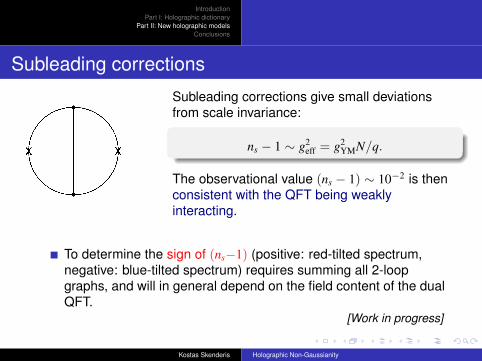
Subleading corrections

Subleading corrections give small deviationsfrom scale invariance:

ns − 1 ∼ g2eff = g2

YMN/q.

The observational value (ns − 1) ∼ 10−2 is thenconsistent with the QFT being weaklyinteracting.

To determine the sign of (ns−1) (positive: red-tilted spectrum,negative: blue-tilted spectrum) requires summing all 2-loopgraphs, and will in general depend on the field content of the dualQFT.

[Work in progress]




2-loop details

Super-renormalizable theories often have infrared problems. Thespecific type of theories we consider however are well-defined: g2

YMacts as an infrared cut-off. [Jackiw, Templeton (1981)] [Appelquist,Pisarski (1981)].The 2-loop integrals are indeed finite and one obtains:

A(q) = CAN2q3[1 + DAg2eff ln q/q0 + O(g4

eff)],

B(q) = CBN2q3[1 + DBg2eff ln q/q0 + O(g4

eff)],

where g2eff = g2

YMN/q and DA and DB are numerical constants.This leads to

nS(q)−1 = −DBg2eff + O(g4

eff), nT(q) = −DAg2eff + O(g4

eff).




Running

Independent of the details of the theory, the scalar spectral indexruns as

αs =dns

d ln q= −(ns−1) + O(g4

eff).

This prediction is qualitatively different from slow-roll inflation, forwhich αs/(ns−1) is of first-order in slow-roll.This prediction is consistent with current data and Planck shouldbe able to either exclude or confirm this running.




WMAP data WMAP Cosmological Parameter Plotter

Solid line:

α = −(ns−1)




Non-GaussianityDirect computation gives

〈T(q1)T(q2)T(q3)〉+∑

i

〈T(qi)T(−qi)〉

− 2(〈T(q1)Υ(q2, q3)〉+ cyclic perms

)= 2CBN2(2q1q2q3 +

∑i

q3i − (q1q2

2 + 5 perms))

Using the holographic formula one finds

B(q1, q2, q3) = BequilNL (q1, q2, q3)

withf equilNL = 5/36

This is independent of all details of theory.This value is larger than the fNL for slow-roll inflation, but probablystill too small to be detected by Planck.




Outline

1 Introduction



4 Conclusions




Conclusions

I have presented a holographic description of inflationarycosmology in terms of a 3-dimensional QFT (without gravity!)When gravity is weakly coupled, holography correctly reproducesstandard inflationary predictions for cosmological observables.When gravity is strongly coupled, one finds new models thathave a QFT description.




Observational signatures

I presented models with the following universal features:

1. they have a nearly scale invariant spectrum of small amplitudeprimordial fluctuations.

2. the scalar spectral index runs as αs = −(ns − 1).3. the three point function of curvature perturbations is exactly

equal to the equilateral form with f equilNL = 5/36.

Both predictions 2 and 3 could easily be ruled out by the Planck datanext year.




Outlook




DW/cosmology correspondence [KS, Townsend (2006)]

FRW spacetime (k = 0,−1,+1)

ds2 = −dt2 + a(t)2(

dr2

1− kr2 + r2(dθ2 + sin θ2dΩ2d−2)

)Curved domain-wall (κ = 0,−1,+1)

ds2 = dz2 + e2A(z)(− dτ 2

1 + κτ 2 + τ 2(dψ2 + sinhψ2dΩ2d−2)

)The analytic continuation

(t, r, θ) = −i(z, τ, ψ)

maps the one solution to the other with

a(t) ↔ eA(z), k ↔ −κ


holography for cosmology - kavli institute for the physics ... · holography for cosmology kostas...

Documents