household finance and the value of life - netspar filemainresults 1....
TRANSCRIPT

Household Finance and the Value of Life
Antoine Bommiera, Daniel Harenberga,François Le Grandb,a
aETH Zurich bEM Lyon Business School
Netspar International Pension WorkshopJanuary 18, 2017

Motivation
• Household finance• Life-cycle models• Savings and portfolio choices• Mortality exogenous• No explicit trade-off between consumption and life duration
• Value of life• Individual willingness to give up consumption for living longer• Cost-benefit analyses of public policies• Focus on estimating statistical value of life
⇒ This paper: import knowledge from value of life literature tohousehold finance literature
Bommier, Harenberg, Le Grand Household Finance and the Value of Life 1/20

Main results
1. Analytic result in stylized 2-period model: if value of life positive,more risk averse agents discount future more and save less
2. Quantitative results in calibrated life-cycle model: if value of lifepositive, more risk averse agents
• save less• participate less in the stock market• if they do, hold smaller share in stock⇒ Overturns important results in previous literature.
3. Empirical result: In SOEP data, more risk averse householdssave less
⇒ Highlights the importance of properly accounting for the value oflife in life-cycle models.
Bommier, Harenberg, Le Grand Household Finance and the Value of Life 2/20

Value of a statistical life
Definition
VSLt =∂U∂pt∂U∂ct
=
individual marginal rate of substitutionbetween survival and consumption at age t
• VSL = individual willingness-to-pay for a small reduction inmortality risk
• To increase her survival probability by 0 < ε� 1, an individualis willing to give up ε× VSLt units of consumption.
• Scaled to one unit of death: 1ε individuals would give up
εVSLtε = VSLt units of consumption to increase the number of
survivors by 1ε × ε = 1.
Bommier, Harenberg, Le Grand Household Finance and the Value of Life 3/20

The VSL in the economics literature
• A whole line of empirical literature estimates the VSL:• by looking at wage-risk trade-offs,• by measuring the willingness to pay for safer cars, homes,. . .• through questionnaires.
• The VSL is a central element:• for many cost-benefit analyses: for example, 85% of the benefits
of the Clean Air Act are related to mortality risk reductions (EPA,2011);
• in the debate about the optimal level of public health expenditure.
• In the USA, the VSL ≈ 7 million USD
Bommier, Harenberg, Le Grand Household Finance and the Value of Life 4/20

A two-period formal example
• Recursive preferences (Kreps-Porteus)
U(c0, c1, p0) = u(c0) + βφ−1Ep0 [φ(U1)],
• φ increasing and concave, controls risk aversion• At = 1:
• If alive, U1 = u(c1)
• If dead, U1 = ud , a constant ∈ [−∞,+∞]
• VSL0 governed by ud : Show formula
VSL0 > 0 ⇔ u(c1) > ud
Bommier, Harenberg, Le Grand Household Finance and the Value of Life 5/20

The discount rate• Definition
δ0 =∂U∂c0∂U∂c1
∣∣∣∣∣c0=c1
− 1
• In our two-period model:
δ0 =1βp0
φ′ (u)
φ′(u(c1))− 1,
where u is a certainty equivalent
u = φ−1 (p0φ(u(c1)) + (1− p0)φ(ud ))
Eg: Without mortality risk: δ0 = 1β − 1
Eg: For additively separable utility (affine φ): δ0 = 1βp0− 1
Bommier, Harenberg, Le Grand Household Finance and the Value of Life 6/20

The discount rate• Definition
δ0 =∂U∂c0∂U∂c1
∣∣∣∣∣c0=c1
− 1
• In our two-period model:
δ0 =1βp0
φ′ (u)
φ′(u(c1))− 1,
where u is a certainty equivalent
u = φ−1 (p0φ(u(c1)) + (1− p0)φ(ud ))
⇒ If VSL > 0: greater risk aversion ⇒ δ0 ↑ → savings ↓ Figure
Bommier, Harenberg, Le Grand Household Finance and the Value of Life 6/20

Risk aversion with several simultaneous risks
• Mortality risk: greater risk aversion ⇒ smaller savings,if VSL > 0
• Labor income risk: greater risk aversion ⇒ greater savings(precautionary motive)
• Financial return risk: depends on IES (see Details )
⇒ Opposing effects and ambiguous overall impact
⇒ Consequences for stock market participation, portfolio choice?
⇒ A quantitative analysis is needed
Bommier, Harenberg, Le Grand Household Finance and the Value of Life 7/20
A quantitative life-cycle model
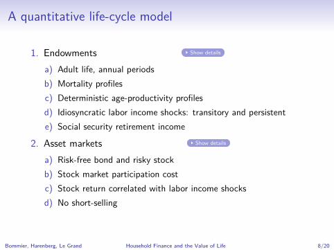
1. Endowments Show details
a) Adult life, annual periodsb) Mortality profilesc) Deterministic age-productivity profilesd) Idiosyncratic labor income shocks: transitory and persistente) Social security retirement income
2. Asset markets Show details
a) Risk-free bond and risky stockb) Stock market participation costc) Stock return correlated with labor income shocksd) No short-selling
Bommier, Harenberg, Le Grand Household Finance and the Value of Life 8/20

Preferences
• Felicity from consumption: u(c) = c1−σ−11−σ
• Felicity from bequests:
v(w) =θ
1− σ[(w + w)1−σ − w1−σ
]− v
• Kreps-Porteus recursive preferences General recursion
UAt =(1− β)u(ct)
+ βΦ−1(
ptEt[Φ(UA
t+1
)]+ (1− pt)Et
[Φ(UD
t+1
)])UD
t = (1− β) v(wt) + βv (0)
Bommier, Harenberg, Le Grand Household Finance and the Value of Life 9/20

Epstein-Zin and risk-sensitive preferences
• Both Kreps-Porteus class Why both?
• Epstein-Zin preferences (EZ), γ controls risk aversion
Φ(u) =1
1− γ (1 + (1− σ)u)1−γ1−σ − 1
1− γ , if γ, σ 6= 1
• γ controls risk aversion
• Risk-sensitive preferences (RS)
Φ(u) = −1k (exp(−ku)− 1) if k 6= 0
• k controls risk aversion
• Limit cases (k = 0, γ = 1, σ = 1) by continuity
Bommier, Harenberg, Le Grand Household Finance and the Value of Life 10/20

Calibration of preferences
1. Calibrate additive agent to empirical savings, VSL, and bequests2. Increase risk aversion for EZ agent3. Calibrate risk aversion of RS agent to match savings of EZ agent
Parameter Value Source/ counterpart/ target
Inverse IES, σ 2.0Exog. endowment, w 1 Net wage y = US$ 21’756Discount factor, β 0.93 Assetsadd
45 = US$ 100’000Life-death gap, v 32.3 VSLadd
45 = US$ 6.5mBequest motive, θ 5.3 Bequestsadd
90 = US$ 50’000†
Risk aversion, EZ, γ 3.0Risk aversion, RS, k 0.09 AssetsRS
45 = AssetsEZ45
Bommier, Harenberg, Le Grand Household Finance and the Value of Life 11/20

Parameterization of endowments and asset marketsParameter Value Source/ counterpart/ target
Working age, retirement age, maximum age 21, 65, 100Survival rates, pt {pt}T
1 U.S. mortality 2007, HMDAge productivity, µt {µt}T
1 Earnings profiles 2007, PSIDAverage wage, y 21 756 USD Net compensation 2007, SSAPensions, yR 33%× y Social security replacement rateAutocorrelation, ρ 0.95 Storesletten, et al. (2004)Var. persistent shocks, σ2
υ 0.03 Storesletten, et al. (2004)—Correlation with stock, κυ 0.15 Gomes and Michaelides (2005)Var. transitory shocks, σ2
ϑ 0.12 Storesletten, et al. (2004)—Correlation with stock, κϑ 0.30 Gomes and Michaelides (2005)Inheritance, w0 0.0
Gross risk-free return, R f 1.02Equity premium, ω 0.03Stock volatility, σν 0.18Participation cost, F 3620 USD
Bommier, Harenberg, Le Grand Household Finance and the Value of Life 12/20
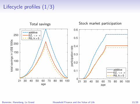
Lifecycle profiles (1/3)
Total savings
age21 30 40 50 60 70 80 90 100
tota
l savin
gs in U
S$ '0
00s
50
100
150
200
250additiveEZ, γ > σRS, k > 0
Stock market participation
age21 30 40 50 60 70 80 90 100
part
icip
ation r
ate
0
0.1
0.2
0.3
0.4
0.5
0.6
additiveEZ, γ > σRS, k > 0
Bommier, Harenberg, Le Grand Household Finance and the Value of Life 13/20

Lifecycle profiles (2/3)
Total savings
age21 30 40 50 60 70 80 90 100
tota
l savin
gs in U
S$ '0
00s
50
100
150
200
250additiveEZ, γ > σRS, k > 0
Conditional Share in Stock
age21 30 40 50 60 70 80 90 100
conditio
nal share
in s
tock
0
0.2
0.4
0.6
0.8
1
additiveEZ, γ > σRS, k > 0
Bommier, Harenberg, Le Grand Household Finance and the Value of Life 14/20

Lifecycle profiles (3/3)
Consumption
age21 30 40 50 60 70 80 90 100
consum
ption in U
S$ '0
00s
10
15
20
25
30
35
40
45
additiveEZ, γ > σRS, k > 0
Value of a Statistical Life
age21 30 40 50 60 70 80 90 100
VS
L in U
S$ '0
00s
×10 4
0
0.5
1
1.5
2
2.5additiveEZ, γ > σRS, k > 0
Bommier, Harenberg, Le Grand Household Finance and the Value of Life 15/20
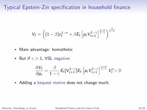
Typical Epstein-Zin specification in household finance
Vt =
((1− β)c1−σ
t + βEt[ptV 1−γ
t+1
] 1−σ1−γ) 1
1−σ
• Main advantage: homothetic
• But if γ > 1, VSL negative:
∂Vt∂pt
=β
1− γEt [V 1−γt+1 ]Et
[ptV 1−γ
t+1
] γ−σ1−γ V σ
t < 0
• Adding a bequest motive does not change much.
Bommier, Harenberg, Le Grand Household Finance and the Value of Life 16/20

Profiles for typical Epstein-Zin specification
Total savings
age21 30 40 50 60 70 80 90 100
tota
l savin
gs in U
S$ '0
00s
50
100
150
200
250
300
350 additiveEZ, γ > σ
Stock market participation
age21 30 40 50 60 70 80 90 100
part
icip
ation r
ate
0
0.1
0.2
0.3
0.4
0.5
0.6
additiveEZ, γ > σ
Bommier, Harenberg, Le Grand Household Finance and the Value of Life 17/20

Supporting evidence
• Empirical analysis based German SOEP• Self-declaration about risk aversion, RA
• 0 ("very willing to take risk") to 10 ("not at all willing to takerisk")
• Dohmen, et al. (2011):• RA good predictor of risky behavior• E. g., smoking, investing in stock, but not savings• Validate with field experiment (N=450)
• Our econometric analysis similar to Fuchs-Schündeln andSchündeln (2005), but with RA as explanatory variable forsavings
Bommier, Harenberg, Le Grand Household Finance and the Value of Life 18/20

Empirical Findings (dependent variable = log(savings))
Explanatory variables W/o interactions With interactions
risk aversion (RA) −0.013*** −0.016***
(0.004) (0.006)
RA × income risk 0.033(0.026)
RA × mortality −0.191*
(0.118)
log(wealth) 0.088*** 0.088***
(0.004) (0.004)
log(permanent income) −0.005 −0.018(0.208) (0.208)
income risk 0.285*** 0.111(0.081) (0.157)
demographic controls Show Show
Nb of observations 22973 22973
Bommier, Harenberg, Le Grand Household Finance and the Value of Life 19/20

Conclusion
• With positive value of life, risk aversion• Amplifies effect of mortality on discounting• Decreases lifecycle savings and stock market participation
• Mortality = main risk in life• Death is a state where you loose (part of) your savings• Saving is risk-taking behavior
• Observed low levels of saving may be rational and explained byhigher risk-aversion
Bommier, Harenberg, Le Grand Household Finance and the Value of Life 20/20

Appendix Table of Contents
Appendix
Household Finance and the Value of Life Appendix 1

Literature 1/2
Risk aversion . . . increases savings . . . decreases savings
Income risk E.g., BCL
Investment risk Kihlstrom and Mirman(1974) and BCL if IES< 1
Kihlstrom and Mirman(1974) and BCL if IES> 1
Mortality risk HPSA if IES < 1 Bommier (2006, 2013),BCL, Drouhin (2015),
HPSA if IES> 1
All three risks Gomes and Michaelides(2005, 2008),. . . more
• BCL: Bommier, Chassagnon, and LeGrand (2012)
• HPSA: Hugonnier, Pelgrin, and St-Amour (2012)
Household Finance and the Value of Life Appendix 2

Literature 1/2
Risk aversion . . . increases savings . . . decreases savings
Income risk E.g., BCL
Investment risk Kihlstrom and Mirman(1974) and BCL if IES< 1
Kihlstrom and Mirman(1974) and BCL if IES> 1
Mortality risk HPSA if IES < 1 Bommier (2006, 2013),BCL, Drouhin (2015),
HPSA if IES> 1
All three risks Gomes and Michaelides(2005, 2008),. . . more
This paper
• BCL: Bommier, Chassagnon, and LeGrand (2012)
• HPSA: Hugonnier, Pelgrin, and St-Amour (2012)
Household Finance and the Value of Life Appendix 2

Literature 2/2• Epstein-Zin preferences:
• With bequests: Gomes and Michaelides (2005), Inkman, Lopez, andMichaelides (2011), Horneff, Maurer, and Stamos (2008a, 2008b)
• Without bequests: Gomes and Michaelides (2008), Gomes,Michaelides, and Polkovnichenko (2009), Fehr and Habermann (2008),Fehr, Habermann, and Kindermann (2008) Fehr, Kallweit, andKindermann (2013)
• Risk aversion and savings:Bommier (2006, 2013), Bommier, Chassagnon, LeGrand (2012), Bhamra
and Uppal (2006)
• Value of a statistical life:Kaplow (2005), Viscusi and Aldy (2003), Bommier and Villeneuve (2012),
Córdoba and Ripoll (2013) Go Back
Household Finance and the Value of Life Appendix 3

VSL in two-period model
• Utility
U(c0, c1, p0) = u(c0) + βφ−1 (p0φ(u(c1)) + (1− p0)φ(ud )) .
• Applying the definition VSLt =∂U∂pt∂U∂ct
yields
VSL0 =β (φ(u(c1))− φ(ud ))
u′(c0)φ′ (φ−1 (p0φ(u(c1)) + (1− p0)φ(ud ))).
Go Back
Household Finance and the Value of Life Appendix 4

Discount rate and risk aversion
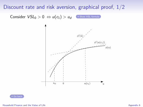
• VSL0 > 0 ⇔ u(c1) > ud Show VSL formula
⇒ ud < u < u(c1)
⇒ φ′(ud ) > φ′(u) > φ′(u(c1)), because φ concave
⇒ φ′(u)φ′(u(c1))
> 1
⇒ amplifies effect of mortality: δ0 = 1βp0
φ′(u)φ′(u(c1))
− 1,
• Risk aversion ↑ ⇒ more concave φ ⇒ stronger amplification⇒ discount rate ↑ ⇒ savings propensity ↓
Show graphical proof Show mathematical proof
Household Finance and the Value of Life Appendix 5

Discount rate and risk aversion, graphical proof, 1/2Consider VSL0 > 0 ⇔ u(c1) > ud Show VSL formula
uud u(c1)
φ(u)
u
φ (u(c1))
φ (u(cd))
E [φ]
Go back
Household Finance and the Value of Life Appendix 6

Discount rate and risk aversion, graphical proof, 1/2Consider VSL0 > 0 ⇔ u(c1) > ud Show VSL formula
uud u(c1)
φ(u)
u
φ′(u(c1))
φ′(u)
φ (u(c1))
φ (u(cd))
E [φ]
Go back
Household Finance and the Value of Life Appendix 6
Discount rate and risk aversion, graphical proof, 1/2Consider VSL0 > 0 ⇔ u(c1) > ud Show VSL formula
uud u(c1)
φ(u)
u
φ′(u(c1))
φ′(u)
Go back
Household Finance and the Value of Life Appendix 6

Discount rate and risk aversion, graphical proof, 1/2Consider VSL0 > 0 ⇔ u(c1) > ud Show VSL formula
uud u(c1)
φ(u)
u
φ′(u(c1))
φ′(u)
φb(u)
Go back
Household Finance and the Value of Life Appendix 6

Discount rate and risk aversion, graphical proof, 1/2Consider VSL0 > 0 ⇔ u(c1) > ud Show VSL formula
uud u(c1)
φ(u)
u
φ′(u(c1))
φ′(u)
φb(u)
ub
φb(ud)
φb (u(c1))
E[φb
]
Go back
Household Finance and the Value of Life Appendix 6

Discount rate and risk aversion, graphical proof, 1/2Consider VSL0 > 0 ⇔ u(c1) > ud Show VSL formula
uud u(c1)
φ(u)
u
φ′(u(c1))
φ′(u)
φb(u)
ub
Go back
Household Finance and the Value of Life Appendix 6
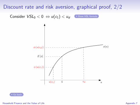
Discount rate and risk aversion, graphical proof, 2/2Consider VSL0 < 0 ⇔ u(c1) < ud Show VSL formula
uudu(c1)
φ(u)
u
φ (u(c1))
φ (u(cd))
E [φ]
Go back
Household Finance and the Value of Life Appendix 7
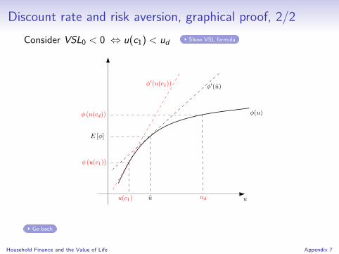
Discount rate and risk aversion, graphical proof, 2/2Consider VSL0 < 0 ⇔ u(c1) < ud Show VSL formula
uudu(c1)
φ(u)
u
φ′(u(c1)) φ′(u)
φ (u(c1))
φ (u(cd))
E [φ]
Go back
Household Finance and the Value of Life Appendix 7

Discount rate and risk aversion, graphical proof, 2/2Consider VSL0 < 0 ⇔ u(c1) < ud Show VSL formula
uudu(c1)
φ(u)
u
φ′(u(c1)) φ′(u)
Go back
Household Finance and the Value of Life Appendix 7

Discount rate and risk aversion, graphical proof, 2/2Consider VSL0 < 0 ⇔ u(c1) < ud Show VSL formula
uudu(c1)
φ(u)
u
φ′(u(c1)) φ′(u)
φb(u)
Go back
Household Finance and the Value of Life Appendix 7

Discount rate and risk aversion, graphical proof, 2/2Consider VSL0 < 0 ⇔ u(c1) < ud Show VSL formula
uudu(c1)
φ(u)
u
φ′(u(c1)) φ′(u)
φb(u)
ub
φb(ud)
φb (u(c1))
E[φb
]
Go back
Household Finance and the Value of Life Appendix 7

Discount rate and risk aversion, graphical proof, 2/2Consider VSL0 < 0 ⇔ u(c1) < ud Show VSL formula
uudu(c1)
φ(u)
u
φb(u)
ub
Go back
Household Finance and the Value of Life Appendix 7
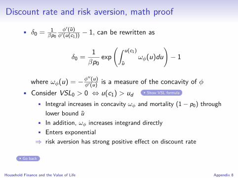
Discount rate and risk aversion, math proof
• δ0 = 1βp0
φ′(u)φ′(u(c1))
− 1, can be rewritten as
δ0 =1βp0
exp(∫ u(c1)
uωφ(u)du
)− 1
where ωφ(u) = −φ′′(u)φ′(u) is a measure of the concavity of φ
• Consider VSL0 > 0 ⇔ u(c1) > ud Show VSL formula
• Integral increases in concavity ωφ and mortality (1− p0) throughlower bound u
• In addition, ωφ increases integrand directly• Enters exponential⇒ risk aversion has strong positive effect on discount rate
Go back
Household Finance and the Value of Life Appendix 8

Savings with uncertain asset returns (go back)
Two periods / two states of the world that determine the asset return.
• Bad state = low return; Good state = high return .• If IES< 1,
• income effect dominates,• sB > sG
• Risk aversion increases savings.• Else if IES> 1,
• substitution effect dominates,• sB < sG ,• Risk aversion decreases savings.
Household Finance and the Value of Life Appendix 9

Endowments
• Working age t = 1 , retirement age T , max age T
• Mortality risk: survival probability pt
• Labor income (1 ≤ t < T )
yLt =y exp(µt + πt + ϑt)
πt =ρπt−1 + υt
ϑtiid∼N
(0, σ2
ϑ
), υt
iid∼ N(0, σ2
υ
)• Social security pension income (T ≤ t ≤ T ), y T
• At t = 1, inherit w0 Go back
Household Finance and the Value of Life Appendix 10

Asset markets
• Bond: risk-free gross return R f
• Stock: risky gross return
lnRst = ln
(R f + ω
)+ νt , νt
iid∼ N(0, σ2
ν
)• νt correlated with both labor income shocks with κϑ and κυ
• No short selling
• Stock-market participation cost, F ≥ 0, paid once in lifeGo back
Household Finance and the Value of Life Appendix 11

Choices and constraints
• Choices {ct , st , bt , ηt}
• Constraints
ct + bt + st + F1ηt=11ηt−1=0 = yt + R f bt−1 + Rst st−1,
st = 0 if ηt = 0,
yt =
yLt if t < T ,
y T else,
ct > 0, bt ≥ 0, st ≥ 0
and bequests are wt = R f bt−1 + Rst st−1.
Household Finance and the Value of Life Appendix 12

General Kreps-Porteus Recursion
• Recursion
Ut = (1− β)ut + βΦ−1(EF×Gt [Φ (Ut+1)]
),
with ut =
u(ct) if alive at t
v(wt) if dead at t
Go Back
Household Finance and the Value of Life Appendix 13

Epstein-Zin and risk-sensitive preferences (2/2)
• EZ: homothetic but not monotone (with respect to FSD)
• RS: non-homothetic but monotone.
⇒ Not monotone, what does that mean? Numerical Example
• RS: the only KP preferences that are monotone and disentanglerisk aversion from IES
• Working paper by Bommier and LeGrand (2014), work inprogress by Bommier, Kochov, and LeGrand (2016))
• In our setting:• Non-monotonicity little impact• Homotheticity has to be given up, because of VSL modelling
Go Back
Household Finance and the Value of Life Appendix 14

Numerical Example of Non-Monotonic Preferences
• Consider EZ utility: V (c0, c1) = c120 + (E[c−
12
1 ])−1.
• Lotteries i = `1, `2 paying off (c i0, c i
d ) or (c i0, c i
u) (50%–50%):
Lottery c i0 c i
d c iu V (c i
0, c id ) V (c i
0, c iu)
i = `1 4 1 7 9.00 21.58
i = `2 2 2.5 9 8.97 19.49
⇒ `1 always pays off more than `2.
• BUT, ex ante, V (c`10 , c`11 ) = 11.91 < 12.15 = V (c`20 , c
`21 )!
Go Back
Household Finance and the Value of Life Appendix 15

Value of a Statistical Life
• Marginal rate of substitution between survival rate andconsumption
VSLt =
∂UAt
∂pt∂UA
t∂ct
⇒ how much consumption to give up for increasing thelikelihood to live another year
Household Finance and the Value of Life Appendix 16

Computation
• Reformulate model• Cash-at-hand, xt = R f bt−1 + Rs
t st−1 + yt
• Total savings, at , and share in stock α ∈ [0, 1]
• Persistent productivity, πt : continuous state variable
• State space (xt , πt , ηt , t)
• Not differentiable
• Standard VFI infeasible
⇒ Use 3D cubic B-spline to interpolate expected continuation value
• Calibration: consider 3 agents: add ,EZ ,RS
Household Finance and the Value of Life Appendix 17

Re-calibration Without Mortality
Parameter Value Source/ counterpart/ target
Inverse IES, σ 2.0Exog. endowment, w 1.5Discount factor, β 0 .96 → 0 .95 Assetsadd
45 = US$ 100’000Life-death gap, v 30 .0 → 30 .3 VSLadd
45 = US$ 6.5mBequest motive, θ 20.0 Bequestsadd
85 =?
Risk aversion, EZ, γ 3.0→ 7.0Risk aversion, RS, k 0.08→ 0.58 AssetsRS
45 = AssetsEZ45
Go Back
Household Finance and the Value of Life Appendix 18

EZ in Gomes and Michaelides 2005
Vt =
(1− βpt)c1− 1ε
t + βEt
(ptV 1−ρ
t+1 + (1− pt)b (Xt+1/b)1−ρ
1− ρ
) 1− 1ε
1−ρ
1
1− 1ε
• Derivative ambiguous if ρ > 1 and ε < 1Go Back
Household Finance and the Value of Life Appendix 19

Re-calibration for ’typical’ EZ Specification
Parameter Value Source/ counterpart/ target
Inverse IES, σ 2.0Exog. endowment, w 1.5Discount factor, β 0.96 Assetsadd
45 = US$ 100’000Life-death gap, v 30.0→ 0.0 not targetedBequest motive, θ 20.0→ 0.0 exogenous
Risk aversion, EZ, γ 3.0→ 7.0Risk aversion, RS, k 0.08→ 0.71 AssetsRS
45 = AssetsEZ45
Go Back
Household Finance and the Value of Life Appendix 20

Controls in estimation
• age, age2, education, education2, gender, marital status (6
values), household size, number of children, current residence
(East or West Germany), year dummies
• R2 = 21.56
Go Back
Household Finance and the Value of Life Appendix 21

References
Bhamra, H. S. and R. Uppal (2006): “The role of risk aversion andintertemporal substitution in dynamic consumption-portfolio choice withrecursive utility,” Journal of Economic Dynamics and Control, 30,967–991.
Bommier, A. (2006): “Uncertain Lifetime and Intertemporal Choice: RiskAversion as a Rationale for Time Discounting,” International EconomicReview, 47, 1223–1246.
——— (2013): “Life Cycle Preferences Revisited,” Journal of EuropeanEconomic Association, 11, 1290–1319.
Bommier, A., A. Chassagnon, and F. Le Grand (2012):“Comparative Risk Aversion: A Formal Approach with Applications toSaving Behaviors,” Journal of Economic Theory, 147, 1614–1641.
Bommier, A., A. Kochov, and F. LeGrand (2016): “On MonotoneRecursive Preferences,” mimeo, ETH Zurich.
Household Finance and the Value of Life Appendix 22

References
Bommier, A. and F. LeGrand (2014): “A Robust Approach to RiskAversion,” Working paper, ETH Zurich.
Bommier, A. and B. Villeneuve (2012): “Risk Aversion and the Valueof Risk to Life,” Journal of Risk and Insurance, 79, 77–104.
Córdoba, J. C. and M. Ripoll (2013): “Beyond Expected Utility in theEconomics of Health and Longevity, Working Paper ,” .
Dohmen, T., A. Falk, D. Huffman, U. Sunde, J. Schupp, and G. G.Wagner (2011): “Individual risk attitudes: Measurement, determinants,and behavioral consequences,” Journal of the European EconomicAssociation, 9, 522–550.
Drouhin, N. (2015): “A Rank-Dependent Utility Model of UncertainLifetime,” Journal of Economic Dynamics and Conctrol, 53, 208–224.
Fehr, H. and C. Habermann (2008): “Risk Sharing and EfficiencyImplications of Progressive Pension Arrangements,” ScandinavianJournal of Economics, 110, 419–443.
Household Finance and the Value of Life Appendix 23
References
Fehr, H., C. Habermann, and F. Kindermann (2008): “Social securitywith rational and hyperbolic consumers,” Review of Economic Dynamics,11, 884–903.
Fehr, H., M. Kallweit, and F. Kindermann (2013): “Should pensionsbe progressive?” European Economic Review, 63, 94–116.
Fuchs-Schuendeln, N. and M. Schuendeln (2005): “PrecautionarySavings and Self-Selection: Evidence from the German Reunification“Experiment”,” Quarterly Journal of Economics, 120, 1085–1120.
Gomes, F. and A. Michaelides (2005): “Optimal Life-Cycle AssetAllocation: Understanding the Empirical Evidence,” The Journal ofFinance, 60, 869–904.
Gomes, F., A. Michaelides, and V. Polkovnichenko (2009):“Optimal savings with taxable and tax-deferred accounts,” Review ofEconomic Dynamics, 12, 718–735.
Household Finance and the Value of Life Appendix 24
References
Gomes, F. J. and A. Michaelides (2008): “Asset Pricing with LimitedRisk Sharing and Heterogeneous Agents,” The Review of FinancialStudies, 21, 415–448.
Horneff, W., R. H. Maurer, and M. Z. Stamos (2008a): “Optimalgradual annuitization: Quantifying the costs of switching to annuities,”Journal of Risk and Uncertainty, 75, 1019–1038.
Horneff, W. J., R. H. Maurer, and M. Z. Stamos (2008b):“Life-cycle asset allocation with annuity markets,” Journal of EconomicDynamics and Control, 32, 3590–3612.
Hugonnier, J., F. Pelgrin, and P. St-Amour (2012): “Health and(Other) Asset Holdings,” The Review of Economic Studies, 80, 663–710.
Inkmann, J., P. Lopes, and A. Michaelides (2011): “How Deep Is theAnnuity Market Participation Puzzle?” Review of Financial Studies, 24,279–319.
Household Finance and the Value of Life Appendix 25

References
Kaplow, L. (2005): “The value of a statistical life and the coefficient ofrelative risk aversion,” Journal of Risk and Uncertainty, 23–34.
Kihlstrom, R. E. and L. J. Mirman (1974): “Risk Aversion with manyCommodities,” Journal of Economic Theory, 8, 361–388.
Storesletten, K., C. I. Telmer, and A. Yaron (2004):“Consumption and Risk sharing over the Life Cycle,” Journal of MonetaryEconomics, 51, 609–633.
Viscusi, W. K. and J. E. Aldy (2003): “The Value of a Statistical Life:A Critical Review of Market Estimates Throughout the World,” TheJournal of Risk and Uncertainty, 27, 5–76.
Household Finance and the Value of Life Appendix 26