how can the heat transfer correlations for finned-tubes
TRANSCRIPT
HAL Id: hal-00699058https://hal.archives-ouvertes.fr/hal-00699058
Submitted on 19 May 2012
HAL is a multi-disciplinary open accessarchive for the deposit and dissemination of sci-entific research documents, whether they are pub-lished or not. The documents may come fromteaching and research institutions in France orabroad, or from public or private research centers.
L’archive ouverte pluridisciplinaire HAL, estdestinée au dépôt et à la diffusion de documentsscientifiques de niveau recherche, publiés ou non,émanant des établissements d’enseignement et derecherche français ou étrangers, des laboratoirespublics ou privés.
How can the heat transfer correlations for finned-tubesinfluence the numerical simulation of the dynamic
behavior of a heat recovery steam generator?H. Walter, R. Hofmann
To cite this version:H. Walter, R. Hofmann. How can the heat transfer correlations for finned-tubes influence the numericalsimulation of the dynamic behavior of a heat recovery steam generator?. Applied Thermal Engineering,Elsevier, 2010, 31 (4), pp.405. 10.1016/j.applthermaleng.2010.08.015. hal-00699058
Accepted Manuscript
Title: How can the heat transfer correlations for finned-tubes influence the numericalsimulation of the dynamic behavior of a heat recovery steam generator?
Authors: H. Walter, R. Hofmann
PII: S1359-4311(10)00342-X
DOI: 10.1016/j.applthermaleng.2010.08.015
Reference: ATE 3208
To appear in: Applied Thermal Engineering
Received Date: 4 January 2010
Revised Date: 12 July 2010
Accepted Date: 15 August 2010
Please cite this article as: H. Walter, R. Hofmann. How can the heat transfer correlations for finned-tubes influence the numerical simulation of the dynamic behavior of a heat recovery steam generator?,Applied Thermal Engineering (2010), doi: 10.1016/j.applthermaleng.2010.08.015
This is a PDF file of an unedited manuscript that has been accepted for publication. As a service toour customers we are providing this early version of the manuscript. The manuscript will undergocopyediting, typesetting, and review of the resulting proof before it is published in its final form. Pleasenote that during the production process errors may be discovered which could affect the content, and alllegal disclaimers that apply to the journal pertain.
How can the heat transfer correlations for finned-tubes
influence the numerical simulation of the dynamic
behavior of a heat recovery steam generator?
H. Waltera,∗, R. Hofmannb
aVienna University of Technology, Institute for Energy Systems and Thermodynamics,
Getreidemarkt 9, A-1060 Vienna, AustriabBERTSCHenergy, Josef Bertsch Gesm.b.H. & Co KG, Herrengasse 23, A-6700
Bludenz, Austria
Abstract
This paper presents the results of a theoretical investigation on the influ-
ence of different heat transfer correlations for finned-tubes to the dynamic
behavior of a heat recovery steam generator (HRSG). The investigation was
done for a vertical type natural circulation HRSG with 3 pressure stages
under hot start-up and shutdown conditions. For the calculation of the flue
gas side heat transfer coefficient the well known correlations for segmented
finned-tubes according to Schmidt, VDI and ESCOATM (traditional and re-
vised) as well as a new correlation, which was developed at the Institute
for Energy Systems and Thermodynamics, are used. The simulation results
show a good agreement in the overall behavior of the boiler between the dif-
ferent correlations. But there are still some important differences found in
the detail analysis of the boiler behavior.
Keywords:
∗Corresponding author. Tel.: +43 1 58801 30218; Fax: +43 1 58801 30299Email address: [email protected] (H. Walter)
Preprint submitted to Applied Thermal Engineering July 12, 2010

Heat transfer correlation, heat recovery steam generator, natural
circulation, finned tubes, numerical simulation
Nomenclature
a Discretization coefficient [kg/s]
aei SIMPLER discretization coefficient for the east neighbor of the cell
i at the staggered grid [kg/s]
aeei SIMPLER discretization coefficient at the east cell boundary of the
east neighbor cell of the cell i [kg/s]
aEi SIMPLER discretization coefficient for the east neighbor of the cell
i [kg/s]
ahE SIMPLER coefficient for the east neighbor cell of the energy balance
for the header [kg/s]
ahP SIMPLER coefficient for the energy balance of the header [kg/s]
ahW SIMPLER coefficient for the west neighbor cell of the energy bal-
ance of the header [kg/s]
amEi SIMPLER pressure correction discretization coefficient for the east
neighbor cell of the cell i [m s]
amhE SIMPLER pressure correction discretization coefficient for the east
neighbor cell of the header [m s]
amhP SIMPLER pressure correction discretization coefficient of the
header [m s]
amhW SIMPLER pressure correction discretization coefficient for the west
neighbor cell of the header [m s]
2

amPi SIMPLER pressure correction discretization coefficient of the cell i
[m s]
amWi SIMPLER pressure correction discretization coefficient for the west
neighbor cell of the cell i [m s]
aPi SIMPLER discretization coefficient for the energy balance of the
cell i [kg/s]
aWi SIMPLER discretization coefficient for the west neighbor of the cell
i [kg/s]
A Cross sectional area [m2]
Amin Net free area of tube row [m2]
Atot Total outside surface area of the finned-tube bundle [m2]
Ab Heating surface of the smooth bare tube [m2]
bei Constant term in discretization equation for the cell i [N]
bh Constant term in discretization equation for the energy balance of
the header [J/s]
bi Constant term in discretization equation for the energy balance of
the cell i [J/s]
bmh Constant term in discretization equation for the header [kg/s]
bmi Constant term in discretization equation for the cell i [kg/s]
bs Average segment width [m]
c General variable [var]
da Bare tube diameter [m]
dei East coefficient of the velocity correction of the cell i [m2s/kg]
dwi West coefficient of the velocity correction of the cell i [m2s/kg]
D Total outside diameter [m]
3

gx Component of the gravity in direction of the tube axis [m/s2]
e Spec. internal energy [J/kg]
F Error [-]
h Spec. enthalpy [J/kg]
hh Spec. enthalpy of the fluid inside the header [J/kg]
H Average fin height [m]
Hs Average segment height [m]
L Average tube length [m]
mg Flue gas mass [kg]
mg Flue gas mass flow [kg/s]
Nf Number of fins per m [1/m]
NL Number of tubes per row [-]
Nr Number of tubes in flow-direction [-]
Nu Nusselt-number [-]
p Pressure [Pa]
∆p Pressure difference [Pa]
ph Pressure of the fluid inside the header [Pa]
pD Drum pressure [Pa]
p′ Pressure correction [Pa]
Pr Prandtl-number [-]
q Heat flux [W/m2]
Re Reynolds-number [-]
s Tube thickness [m]
sf Average fin thickness [m]
4

Seci Constant term of the linearized source term of the cell i [Pa/m]
SeP i Proportional term of the linearized source term of the cell i [Pa
s/m2]
Sch Constant term of the linearized source term for the energy balance
of the header [W/m3]
SPh Proportional term of the linearized source term for the energy bal-
ance of the header [kg/m3s]
Sci Constant term of the linearized source term for the energy balance
of the cell i [W/m3]
SPi Proportional term of the linearized source term for the energy bal-
ance of the cell i [kg/m2s]
tf Fin pitch [m]
tl Longitudinal tube pitch [m]
tt Transversal tube pitch [m]
T Temperature [K]
Tf Mean fin temperature [K]
Tg Mean gas temperature [K]
U Perimeter [m]
Vh Volume of the fluid inside the header [m3]
w Fluid velocity [m/s]
w Pseudo-fluid velocity [m/s]
x Length [m]
α Heat transfer coefficient [W/m2K]
Density [kg/m3]
h Density of the fluid inside the header [kg/m3]
ϑ Temperature []
5

η Dynamic viscosity [Pa s]
τ Time [s]
ζ Pressure loss coefficient [-]
Superscripts
0 Value at the old time step
∗ Approximate value
′ Correction value
ˆ Pseudo value
Subscripts
0 Characteristic length at da
b Bare tube
E East grid point in mass and energy balance
ESCt ESCOA traditional
f Fin
fric Friction
g Gas
h Header
i Counter for the heat transfer correlations
in Inlet
j Index, counter
k Index, counter
l Longitudinal
m Mass
6
max Maximum
min Minimum
N Index, counter
P Grid point in mass and energy balance
rel Relative
r Tube row
s Segment
t Transversal
tot Total
wa wall
W West grid point in mass and energy balance
1. Introduction
In the energy and process technology most of the high power steam gen-
erators are designed as water tube boilers. Many of these boilers use the
waste heat of gas turbines. In these so called combined power cycles the
steam generator is arranged downstream the gas turbine (GT). Modern gas
turbines for combined cycles are highly flexible in their mode of operation,
i.e., concerning rates of start up, load change and shutdown. Heat Recovery
Steam Generators (HRSG) arranged downstream of the GT are forced to
operate in such a way, that the gas turbine operation is not restricted by
them. Therefore, they should be designed for a high cycling capability with
typical values in the range of approx. 250 cold starts, 1000 warm and 2500
hot starts for their typical 25 year life span.
Modern heavy duty GT are characterized by short start up times and high
7
load change velocities. Both during a cold and warm start these GT achieve
100% of their nominal load in approx. 20 minutes, while 70% of the nominal
GT-exhaust gas temperature and 60% of the nominal exhaust gas flow is
already achieved approx. 7 minutes after the GT start. The downstream
arranged HRSG is supposed not to hinder the operation and load change
velocity of the GT. Especially for vertical type HRSG with horizontal tubes
in the evaporator the requirements posed by the GT demand an accurate
calculation and a detailed engineering of the dynamic behavior of the HRSG.
The combined cycle power plant reaches its nominal load 120 or 190 minutes
after the GT start, depending upon whether warm- or cold-start is performed.
For a compact design of the HRSG finned-tubes are used for the bundle
heating surfaces.
Careful engineering and accurate prediction and simulation tools are nec-
essary in order to ensure an unhindered operation of the GT and take advan-
tage of the many positive aspects of the HRSG design. In Europe many of
these HRSG boilers are designed as vertical type with an natural circulation
evaporator. Normally, the fluid in the natural circulation evaporator flows
from the downcomer through the heated tube bank straight to the riser. The
driving force of the natural circulation is generated due to the density dif-
ference of the water in the downcomer and the water/steam mixture in the
tube bank and the riser tubes. The experience shows, that the most critical
operation modes of HRSG’s with a natural circulation evaporator are fast
warm start-ups and heavy load changes. In these cases stagnation and/or
reverse flow can occur due to dynamic effects (see e.g. [1, 2, 3]). In order to
avoid such situations it is important to have some information about the flow
8
distribution in the tube network of the steam generator available already in
the stage of boiler design. To get some important informations it is neces-
sary to have validated simulation tools which allow to calculate the start-up
and/or shutdown behavior of boilers.
It is well known that the influence of the flue gas heat transfer coefficient
to the overall heat transfer coefficient is higher compared to the heat transfer
coefficient of the working medium (in case of a boiler water, steam or a
water/steam mixture). For this reason the heat transfer coefficient between
flue gas and tube wall has an important influence on the heat flux - and in the
last consequence - on the dynamic behavior of heat exchangers respectively
steam generators.
Finned-tubes which are used in many HRSG’s have geometrically a sim-
ilar design e.g. helical solid or segmented finned-tubes et cetera. For such
types of finned-tubes there are a higher number of heat transfer correlations
available in the literature. But these correlations are measured under differ-
ent conditions (definition region for Re and Pr-numbers) and with different
tube geometry (e.g. fin pitch, bare tube diameter, number of fins per meter,
et cetera).
In computer codes one or more of such heat transfer correlations are
implemented. But the range of validity of these correlations can but must
not agree with the tubes installed in the boiler as well as in the range of
the analyzed operation mode e.g. start-up or shutdown (where Re can go to
zero).
In the present paper the results of a theoretical investigation on the in-
fluence of different heat transfer correlations for finned-tubes to the dynamic
9

behavior of a HRSG will be presented. The investigation was done for a
vertical type natural circulation heat recovery steam generator with 3 pres-
sure stages under hot start-up and shutdown conditions. For the calculation
of the flue gas side heat transfer coefficient the well known correlations for
segmented finned-tubes according to Schmidt [4], VDI [5] and ESCOATM
(traditional and revised) [6, 7] as well as a new correlation, which was de-
veloped at the Institute for Energy Systems and Thermodynamics [8, 9], are
used.
2. Brief description of the mathematical model and numerical method
To analyze the dynamic behavior of the natural circulation HRSG the
computer program DBS (Dynamic Boiler Simulation), which was developed
at the Institute for Energy Systems and Thermodynamics (IET) at the Vi-
enna University of Technology [10, 11], was used. The discretization of the
partial differential equations for the conservation laws was done with the aid
of the finite-volume-method. The pressure-velocity coupling and overall so-
lution procedure are based on the pressure correction algorithm SIMPLER
(Semi Implicit Method for Pressure Linked Equations Revised) [12]. To
prevent checkerboard pressure fields a staggered grid is employed and for
the convective term the UPWIND scheme is used. In the following a short
description of the mathematical model for the fluid flow in the tubes and the
headers (the so called ”tube-header-model”) will be presented.
2.1. Model of the fluid flow in the tube
The mass flow in the tubes of a steam generator can be assumed to be
one-dimensional, as the length of the tubes is much larger compared to their
10
diameter. For the model under consideration, the topology of the tube net-
work, the number of parallel tubes, the geometry in terms of outer diameter
and wall thickness of the tubes, the fin geometry and the dimensions of the
gas ducts are necessary. Furthermore, the thermodynamic data - such as
mass flow, pressure and temperature - of the heat exchanging flows are used
as input data.
The mathematical model [10] for the working medium is one-dimensional
in flow direction and uses a homogeneous equilibrium model for the two-
phase flow and applies a correction factor for the two phase pressure loss
according to Friedel [13]. For a straight tube with constant cross section the
governing equations in flow direction are written for the mass and momentum
conservation of the fluid:
∂
∂τ+
∂ (w)
∂x= 0 (1)
∂ (w)
∂τ+
∂ (w w + p)
∂x=
∂
∂x
(
η∂w
∂x
)
− gx −
(
∂p
∂x
)
fric
(2)
The density and the velocity w are averaged values over the cross section
of the tube.
Considering the fluid flow in steam boilers, the thermal energy is much
higher than the kinetic and the potential energy as well as the expansion
work. Therefore, the balance equation for the thermal energy can be simpli-
fied with the help of
e = h−p
(3)
to:∂ ( h)
∂τ+
∂ ( h w)
∂x= q
U
A+
∂p
∂τ. (4)
11
The heat exchange between the fluid and the tube wall is governed by
Newton’s law of cooling and the heat transfer through the wall is assumed
to be in radial direction only. The heat transfer models used in DBS for the
single and two-phase flow of the working medium includes correlations for
horizontal as well as for vertical tubes and is described in detail in [10].
2.2. Model of the header
The header is one of the most important structural component of every
steam generator and is used to connect a low number of connection tubes
with a large diameter and the high number of tubes of a bundle heating
surface or a combustion wall with a small tube diameter.
Figure 1 shows a header and the connected tubes. The three connected
tubes are representative for all the other tubes which are connected to the
header. Index j denotes the tubes where the mass flow enters the header,
while index k indicates the tubes where the mass flow leaves the header. The
index h denotes the thermodynamic state variables of the header.
For the computations of the header, the following assumptions may be
made:
• Assuming that the distribution of the thermodynamic state of the
header is homogeneous, the collector can be seen as one control vol-
ume for the calculation.
• The gravity distribution of density and pressure of the fluid inside the
header can be neglected because the vertical dimension of the header
is small compared to that of the remaining tube system.
12
• The huge difference in the cross section area of the header and the
connected tubes causes strong turbulence, avoiding thus a segregation
of the fluid in the header.
Because the headers are assumed to be a single control volume, the equa-
tions for the mass and energy balance are ordinary differential equations with
time τ as independent variable:
d (h Vh)
dτ=
∑
j
j wj Aj −∑
k
k wk Ak (5)
d (h hh Vh)
dτ=
∑
j
j wj hj Aj −∑
k
k wk hk Ak (6)
The variables of the header are denoted with the index h; j represents
values at the header entrance and k the values at the outlet. Vh is the volume
of the fluid inside the header and A the cross sectional area of the connected
tubes. Similar to the treatment of the fluid flow in the tube, the kinetic
energy as well as the expansion work is neglected in the energy balance.
Because momentum is a vector quantity, having the direction of the tube
axis, the momentum fluxes must not be added arithmetically but rather as
vectors. This is the case at the inlet and outlet of the headers, where the
individual tubes are connected under different angles. But the velocity of the
fluid inside the header is rather small compared to that inside the tubes. So
it can be assumed that the momentum of the fluid will be lost at the inlet of
the header and has to be rebuilt at the outlet. Based on this assumption, the
momentum balance of the header reduces to a pressure balance. The changes
of the momentum at the inlet and the outlet can be taken into account by a
13

pressure loss coefficient ζ:
ph = pj −ζj
2j wj |wj| (7)
ph = pk +ζk
2k wk |wk| . (8)
ζk takes into account the sum of the pressure loss due to the acceleration
of the fluid inside the header from approx. zero to the tube inlet velocity and
the frictional pressure loss across the sudden contraction. The pressure loss
for e.g. a sharp-edged entrance can be found in [14] or [15] and is identical
0.5. ζj represents the frictional pressure loss of the fluid flowing from the
tube outlet cell into the header. Based on the model assumptions for the
header the recovery of the pressure energy from the kinetic energy of the
fluid is set to zero.
Based on the simplifications described above, the algebraic equations for
header and header connected tubes will be presented in the next section. The
description of the tube-header model is written for readers who are familiar
with the basic ideas and notations of the well known SIMPLER method [12].
2.2.1. Discretized balance equations for the header
Taking into consideration the above described tube-header-model the dis-
sipation and regeneration of the momentum leads to separation of the mo-
mentum balance for the header connected tubes. At the formulation of the
momentum equations for the single control volumes of the tube network the
control volume of the header can be neglected. So, the calculation of the
pseudo-velocity w for the control volume of the header can be neglected and
the tri-diagonal structure of the matrix for the momentum balance can be
14
preserved. Compared to the calculation of the pseudo-velocity the calcula-
tion of the header pressure must include the control volume of the header,
because the pressure of the header even depends on the neighbor cells. The
pressure equation for the header leads to:
amhP ph =∑
j
amhW,j pN,j +∑
k
amhE,k p1,k + bmh (9)
with the coefficients:
amhP =∑
j
amhW,j +∑
k
amhE,k, (10)
amhW,j = (A)N+ 1
2,j dwN,j , (11)
amhE,k = (A)0+ 1
2,k de1,k, and (12)
bmh =(0
h − h)Vh
∆τ+∑
j
(wA)N+ 1
2,j −
∑
k
(wA)0+ 1
2,k. (13)
The pressure correction equation of the header for calculating the velocity
correction can be formulated as follows:
amhP p′h =∑
j
amhW,j p′N,j +∑
k
amhE,k p′1,k + bmh. (14)
The coefficients for Eq. (14) are identical to the Eq. (10) to (13). Just
the pseudo-velocity w in Eq. (13) must be changed by the approximated
velocity w∗.
The conditional equation for the spec. enthalpy of the fluid inside the
header hh can be calculated with
ahP hh =∑
j
ahW,j hN,j +∑
k
ahE,k h1,k + bh (15)
15
with the coefficients:
ahP =∑
j
ahW,j +∑
k
ahE,k + a0hP − SphVh, (16)
ahW,j = max[(w)N+ 1
2,j, 0] AN+ 1
2,j, (17)
ahE,k = max[−(w)0+ 1
2,k, 0] A0+ 1
2,k, (18)
bh = SchVh + a0hP h0
h and (19)
a0hP =
0hVh
∆τ. (20)
2.2.2. Discretized balance equations for the header connected control volumes
In this section, the discretized balance equations for the header connected
control volumes will be presented. The number of control volumes which are
connected to the header are not restricted by the model. The numbering of
the header connected control volumes can be seen in Fig. 1. All equations
are independent from the flow direction.
With the following equations the pressure, velocity and the spec. enthalpy
for the control volume 1, k at the tube inlet can be calculated. The equations
for the pseudo-velocity for the control volume 0 of the tubes k, k + 1, etc.
leads to:
w0+ 1
2,k =
aee0,kw1+ 1
2,k + be0,k
ae0,k
(21)
with the coefficients:
ae0,k = aee0,k + a0e0,k − Sep0,kA0+ 1
2,k∆x0+ 1
2,k (22)
aee0,k =
(
η1+ 1
2,k
∆x1+ 1
2,k
+ max[
−(w)1+ 1
2,k, 0]
)
A1+ 1
2,k, (23)
be0,k = Sec0,k A0+ 1
2,k ∆x0+ 1
2,k + a0
e0,k w0
0+ 1
2,k
and (24)
a0e0,k =
0
0+ 1
2,k
A0+ 1
2,k ∆x0+ 1
2,k
∆τ. (25)
16
The proportional part of the source term leads to:
Sep0,k∆x0+ 1
2,k = −
|∆pfric 0+ 1
2,k|
|w0+ 1
2,k|
− (1+ ζin)0+ 1
2,kw0+ 1
2,k max[w0+ 1
2,k, 0]
2∣
∣
∣w0+ 1
2,k
∣
∣
∣
. (26)
With the factor ζin the pressure loss due to the acceleration of the fluid
inside the header from approx. zero to the tube inlet velocity is considered.
For a sharp-edged entrance the pressure loss coefficient ζin is identical to 0.5
according to [14]. In case of reverse flow at the tube inlet the pressure loss
due to acceleration will be identical to zero with the help of the operator
max[A,B]. This is consistent with the model assumption where the momen-
tum of the fluid will be lost at the inlet of the header. In this case the fraction
of the decrease in kinetic energy which will be recovered by an increase in
pressure energy must not be taken into consideration.
The discretized equation for the pressure of the first control volume 1, k
yield to:
amP1,k p1,k = amW1,k ph + amE1,k p2,k + bm1,k (27)
with the coefficients:
amP1,k = amW1,k + amE1,k, (28)
amW1,k = (A)0+ 1
2,k dw1,k, (29)
amE1,k = (A)1+ 1
2,k de1,k and (30)
bm1,k =(0
1,k − 1,k)A1,k∆x1,k
∆τ+ (wA)0+ 1
2,k − (wA)1+ 1
2,k. (31)
The momentum balance for the staggered control volume 0, k can be
calculated with the help of the new pressure field and results to:
ae0,k w∗0+ 1
2,k
= aee0,k w∗1+ 1
2,k
+ be0,k + (ph − p1,k)A0+ 1
2,k. (32)
17
The coefficients for Eq. (32) can be calculated with the help of Eq. (22)
to (25).
The pressure correction equation for determination of the velocity field
can be written for the control volume 1, k independent from the direction of
the fluid in the tube channel in the following form:
amP1,k p′1,k = amW1,k p′h + amE1,k p′2,k + bm1,k. (33)
The coefficients for Eq. (33) are equivalent to the Eq. (28) to (31). Just
the pseudo-velocity w must be changed in Eq. (31) by the approximated
velocity w∗.
The energy balance for the control volume 1, k is given with:
aP1,k h1,k = aW1,k hh + aE1,k h2,k + b1,k (34)
with the coefficients:
aP1,k = aW1,k + aE1,k + a0P1,k − Sp1,kA1,k∆x1,k (35)
aW1,k = max[(w)0+ 1
2,k, 0] A0+ 1
2,k, (36)
aE1,k = max[−(w)1+ 1
2,k, 0] A1+ 1
2,k (37)
b1,k = Sc1,kA1,k∆x1,k + a0P1,kh
01,k and (38)
a0P1,k =
01,kA1,k∆x1,k
∆τ. (39)
The equations for the first control volumes at the tube outlet (subscript
N) are similar to the equations presented above. Therefore they are not de-
scribed here in detail. This set of equations can be derived from the equations
(21) to (39).
A more detailed description of the tube-header model as well as for the
model of the drum and controller can be found in [10, 11, 16] and [17].
18
2.3. Model for the flue gas
For the mathematical description of the flue gas the one-dimensional par-
tial differential equation of the conservation law for the energy and mass is
used. The mass balance for the flue gas is calculated quasi-stationary, while
for the energy balance the following simplified balance equation is used:
∂ (mg hg)
∂τ+ ∆x
∂ (mg hg)
∂x=
k∑
j=1
αgjAO,waj (ϑWaj − ϑg) . (40)
The discretization of the energy balance is done corresponding to the
finite-volume-method. The momentum balance for the flue gas is neglected,
because the computer code will not be used for calculating pressure fluctua-
tions in the flue gas pass.
The convective heat transfer coefficient between the flue gas and the tubes
can be calculated in DBS with different correlations for smooth or finned,
inline, or staggered tube banks. A brief description of the heat transfer
correlations used in this investigation is given in the Section 3.
2.4. Physical properties
For the numerical calculation of the fluid flow in steam generators the
thermodynamic- and transport properties for water and steam, the flue gas
as well as for the pipe material are needed. In general the properties are
dependent from the state variables pressure and temperature. While the
pressure dependency of water and steam is very high, the dependency on
pressure for the flue gas and the pipe material can be neglected. This sim-
plification for the flue gas can be done due to the fact that all processes take
place at approx. atmospheric pressure conditions.
19
The calculation of the thermodynamic- and transport properties in DBS
are done with correlations from the open literature. For water and steam
the equations according to [18], for the flue gas the correlations according
to [19] and for the pipe material the formulas according to [20] are used. In
addition to the temperature the properties for the flue gas depends also on
the flue gas composition, which is an input parameter in DBS.
3. Analyzed finned-tube correlations
3.1. Correlation according to Hofmann
Experimental investigations are performed at different finned-tube bundle
configurations, at the Institute for Energy Systems and Thermodynamics [9].
The tube bundles were arranged at equal transverse pitch, and in case of
up to eight consecutively arranged tubes, with equal longitudinally pitch in
staggered formation. Thus, a maximum total number of 88 tubes in different
configurations are investigated. All investigations are accomplished under hot
conditions, so that the effect of the pressure recovery through the tube bundle
has to be considered, as well as ambient temperature conditions without any
pressure recovery. The Reynolds-number related to the bare tube diameter
is varied in the range between 4500 and 35000. The geometrical data of the
tube and the arrangement in the test channel is summarized in Table 1.
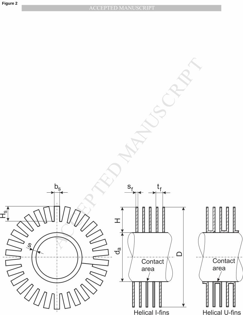
The profile of the helical finned-tubes used is depicted in a schematic
sketch in Fig. 2. Therein the fin pitch tf is 1
Nf, bs is the average segment
width, Hs the average segment height, sf the average fin thickness, H the
average fin height, s the tube thickness, and D = da + 2H, with da as the
bare tube diameter.
20
The geometrical dimensions of the investigated tubes are equal to real
industrial scale. The main idea of the investigated U-shaped finned-tube
is a larger contact area between fin and tube, compared to I-shaped fins.
The measurements were accomplished at the gas-side and at the waterside
respectively. Apart from describing the functional connections of the mea-
surements, the scope of a performed validation should be addressed to fulfill
the energy balance of the used system boundaries. Each heat transfer mea-
surement series is performed to attempt high accuracy. To obtain precise heat
transfer correlations, each calculated point was validated after measurement.
The applied data validation model, shown in [21], was introduced by Tenner
et al. [22]. This curve-fitting technique utilizes equations for mass and energy
balances as well as measurement value equations. For the analysis of mea-
surements a uncertainty calculation is a sufficient condition. According to
DIN 1319, [23], the propagation of uncertainties was calculated. As a result
of measurements at different tube row configurations, a reduction coefficient
for the heat transfer from the finned-tubes was derived [8]. As a result of
the experimental investigations new equations for calculating the Nusselt-
number Nu and pressure drop coefficient ζ are developed. The heat transfer
at segmented finned-tubes at staggered layout at constant Pr is suggested
to be empirically correlated with the following correlation, [9]:
Nu0,Nr= 0.36475 ·Re0.6013Pr1/3
[
1− 0.392 log
(
Nr,∞
Nr
)]
, (41)
21
within range of validity
Pr ≈ 0.71
4500 ≤ Re ≤ 35000
15.5 mm ≤ H ≤ 20 mm
0.8 mm ≤ sf ≤ 1.0 mm
1/295 ≤ tf ≤ 1/276 fins / m
1 ≤ Nr ≤ 8
According to [24] and [8], the Nusselt-number Nu01 is correlated for Nr
consecutive tube rows, with Nr less than 8 for the investigated I/U-fin tubes,
where ∞ at Nr = 8. A comparison of the proposed equation for the Nusselt-
number with almost all measurement results are found to be accurate within
about 20%. The deviation between 50% of all measurement results and the
Eq. (41) are correlated within 5%. Approx. 80% of the measurements have
a relative uncertainty laying within 15%. For further details regarding the
calculation procedure it is referred to [9].
3.2. Calculation according to ESCOATM
Further equations for determination of the external heat transfer coef-
ficient at helical solid and segmented finned-tubes in cross-flow, arranged
in-line and staggered, are provided by ESCOATM (Extended Surface Corpo-
ration of America), [6, 7]. The basis of these equations are measurements
performed by e.g. Weierman [25]. As stated in [6] both, the well known tra-
ditional ESCOATM -correlations and the new revised ESCOATM -correlations
1calculated with the bare tube diameter
22
for segmented finned-tubes at staggered arrangement are defined as follows:
Nu0 = C1C3C5RePr1/3
(
Tg
Tf
)0.25(D
da
)0.5
. (42)
Therein Tg is the mean gas temperature, Tf is the mean fin temperature and
D the finning diameter, which is D = da + 2H. The coefficients C1, C3, and
C5 are defined with:
3.2.1. Traditional ESCOATM -Correlation
C1 = 0.25Re−0.35, (43)
C3 = 0.55 + 0.45 exp
(
−0.35 H
tf − sf
)
, (44)
C5 = 0.7 +[
0.7− 0.8 exp(−0.15N2r )]
exp
(
−tltt
)
. (45)
3.2.2. Revised ESCOATM -Correlation
C1 = 0.091Re−0.25, (46)
C3 = 0.35 + 0.65 exp
(
−0.17 H
tf − sf
)
, (47)
C5 = 0.7 +[
0.7− 0.8 exp(−0.15N2r )]
exp
(
−tltt
)
. (48)
The coefficient C3 is a factor specifying the influence of the fin height and the
fin distance; C5 considers the influence of the transversal and the longitudi-
nal pitch within the finned-tube bundle as well as the number of consecutive
tubes in cross-flow. As characteristic length, the bare tube diameter is con-
sidered. The heat transfer equations of Weierman [25] show an evaluated
23
measurement uncertainty of about ±10% for segmented finned-tubes in a
equilateral staggered layout. Range of validity [25, 7]:
≈ (2000 ≤ Re ≤ 500000)
9.5 mm ≤ H ≤ 38.1 mm
0.9 mm ≤ sf ≤ 4.2 mm
1 ≤ tf ≤ 7 fins/inch
3.3. Calculation according to Th. E. Schmidt
According to Schmidt [4], in terms of significance, the bare tube diameter
as the characteristic length for determining the heat transfer coefficient is
taken into account. The correlation is evaluated from a large number of
test cases, mostly with annular solid fins and result in lower heat transfer
coefficients than spiral fins. The correlation in case of staggered tube layout
is defined with:
Nu0 = 0.45Re0.625Pr1/3
(
Atot
Ab
)
−0.375
. (49)
This heat transfer correlation is valid for an evaluated measurement uncer-
tainty of about ±25%, 1000 ≤ Re ≤ 40000, 5 ≤ Atot
Ab≤ 12 and Nr ≥ 3
consecutive arranged tube rows. As stated in [26, 4] Atot is the entire gas-
affected heating surface per m tube and Ab is the heating surface of the
smooth bare tube per m.
3.4. Calculation according to VDI-Heat Atlas
An equation for evaluating the heat transfer at staggered finned-tube bun-
dles is specified in the VDI Heat-Atlas, 10th edition, [5]. As compared in [26],
this equation is very similar to the correlation of Th.E. Schmidt, but other
24
coefficients and exponents are evaluated. All correlations are based on the
bare tube diameter da as characteristic length. If the flooding length, equiv-
alent diameter in volume, or hydraulic diameter is used as the characteristic
length, both the Nu-number and the Re-number have to be converted. The
equation in case of staggered tube layout reads as
Nu0 = 0.38Re0.6Pr1/3
(
Atot
Ab
)
−0.15
(50)
and is valid for Nr ≥ 4 consecutive arranged tube rows. In case of Nr = 3
tube rows the constant in the power law evaluates for 0.36, and if Nr = 2
the constant follows too 0.33. This heat transfer correlation is valid for an
evaluated measurement uncertainty of about ±10% to ±25%, 1000 ≤ Re ≤
100000 and 5 ≤ Atot
Ab≤ 30.
4. Simulated heat recovery boiler
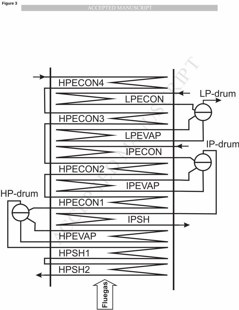
Figure 3 shows a sketch of the overall design of the simulated vertical
type natural circulation three pressure stage HRSG. The drum pressure at
full operation load for the high pressure system (HP) is 125 bars, for the
intermediate pressure system (IP) 39 bars and for the low pressure system
(LP) 12.8 bars. The HP-system consists of four economizer (HPECON1-4),
an evaporator (HPEVAP) with 6 parallel tube paths and two super heaters
HPSH1 and HPSH2, whereas HPSH1 has two parallel tube paths. The IP-
system consists of an economizer (IPECON), an evaporator (IPEVAP) with
3 parallel tube paths and a super heater (IPSH) and the LP-system consists
of an economizer (LPECON) and an evaporator (LPEVAP) with 3 parallel
tube paths. The saturated steam of the LP-system is used by another process
25
and will not be superheated. In the simulation model all parallel tube paths
are included. The flue gas enters the flue gas pass of the boiler at the bottom
and leaves it at the top.
Some important geometric data for the investigation of the analyzed
HRSG boiler are summarized in Tab. 2. All tubes of the bundle heating
surfaces are serrated finned-tubes with an bare tube diameter of ∅38.1 mm,
an averaged fin thickness of 0.8 mm and an averaged fin segment width of 4
mm. The tube rows of all heating surfaces are arranged in a staggered way
with a longitudinal pitch of 79 mm and a transversal pitch of 92 mm. The
heated length of the horizontal tubes per layer was 20 m.
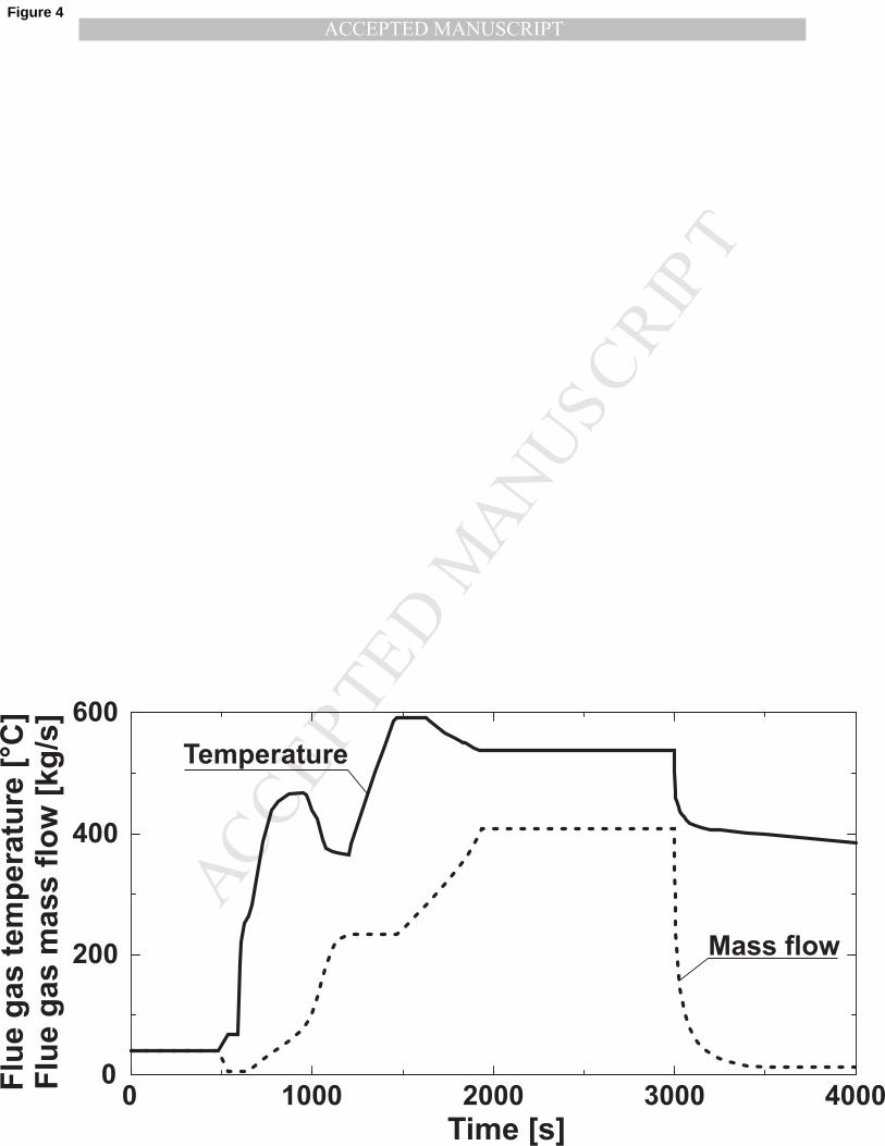
The GT exhaust flue gas mass flow and temperature, which are boundary
conditions for the simulations, are given as a function of time and can be
shown in Fig. 4. The total simulation time was 9500 s.
During the first period of the simulation (480 s) the GT purges the boiler.
After synchronization (between 480 and 540 s) the GT starts and reaches full
load 1950 s after simulation start. In the time period between 1950 and 3000
s the GT works under full load operation condition. Following the stationary
operation at full load the shutdown of the GT is simulated between 3000 and
9500 s. In this period the GT exhaust mass flow decreases rapidly close to
zero, while the exhaust temperature decreases approx. linearly with a small
gradient (see Fig. 5).
The exhaust flue gas mass flow from the gas turbine during the simulated
shut down period is not identical zero, because in the reality the gas turbine
rotor is turned at low rpm (revolutions per minute) for a controlled turbine
engine cool down, to allow an instant restart during this time period.
26
4.1. Initial and boundary conditions for the numerical simulation
The start-up behavior of a boiler depends on the time difference between
the shutdown and restart. A start-up from the cold load - (the system pres-
sure in the drum is equal to the atmospheric pressure) or part load condition,
the admissible rate of pressure (temperature) change of the natural circula-
tion system is mostly conditioned by the thermal stresses of the large diam-
eter components, which are positioned in the saturation region of the boiler,
e. g. cyclones inside the drum used for the water/steam separation, head-
ers and drum. This limitation applies both to load increase and reduction.
Therefore the natural circulation system is only applicable for a variable pres-
sure operation under certain conditions. Because a load change linked with
a pressure change is accompanied by a change of the saturation temperature.
Especially in the low pressure region the change of the saturation temper-
ature is high. Tables with a start-up time for drums, cyclones and headers
for different design pressures and wall thickness can be seen in [27]. The
simulation of the analyzed boiler was done under hot start-up conditions. In
this case the time difference between the shutdown and restart of the HRSG
boiler is up to approx. one full day (overnight standstill). The operation
pressure does not change during this time. Therefore the limitation of the
pressure (temperature) change is not taken into account and the boiler can
start in a faster way.
For the simulation of the boiler the following initial conditions are used:
• The steam generator is filled with water near boiling condition.
• The pressure distribution of the working medium in the tube network
of the boiler is affected by gravity.
27
• The velocity of the fluid at the start of the calculation process is equal
to zero.
• The initial fluid temperature in the evaporator of the boiler is identical
to the boiling temperature at drum pressure.
• The initial drum pressure for the HP-system was 100 bars, for the IP-
system 32 bars and for the LP-system 12 bars.
• The water level in the different drums at simulation start is located at
low water level.
5. Results of the numerical simulation
Before presenting the simulation results calculated with the different heat
transfer correlations for finned-tubes a brief description of the general start-
up behavior of the boiler will be given. This calculation is done with the
traditional ESCOATM correlation.
5.1. Start-up behavior of the boiler
Based on the development of the gas turbine exhaust flue gas mass flow
and temperature the operation pressure of the different drums change. Dur-
ing the purging of the HRSG and the synchronization of the GT (first 540
s of simulation, see Fig. 4) the drum pressure of the HP-system decreases
approx. linear down to 89 bars, the IP-system to 28.3 bars while the drum
pressure of the LP-system is approx. constant. This behavior of the pressure
is a result of the heat transfer from the working fluid in direction to the flue
gas mass flow (cooling of some of the HRSG heating surfaces, e.g. HPSH1
28
and HPSH2). Between approx. 540 s and 1200 s after simulation start the
drum pressures are approx. constant followed by an increase of the HP drum
pressure with 3 bars/min, the IP drum pressure with 0.88 bars/min and the
LP drum pressure with 0.05 bars/min up to the different pressure values at
full load. After achieving the system pressure at full operation load the drum
pressures are approx. constant.
Figure 5 shows the development of the flue gas temperature at the GT
outlet as well as in front of the evaporator of the different pressure stages. It
can be seen, that during the purging process and the first period of the GT
start-up the flue gas temperature before the different evaporators is higher
than the GT outlet temperature. Therefore the flue gas is heated up and the
tubes of some of the heating surfaces are cooled down during these periods.
This can be seen also at the GT shutdown at the HP-system.
The total absorbed heat flow from the boiler under full operation condi-
tion is approx. 175 MW.
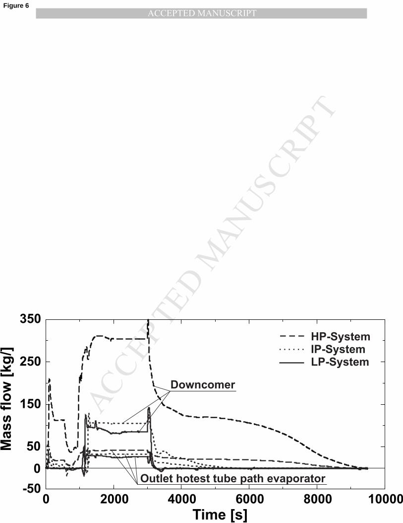
Figure 6 shows the mass flow in the downcomer and at the outlet of
the highest heated tube path of the different evaporators. In the following
the development of the mass flow in the HP evaporator (HPEVAP) will be
described in detail. During the purging period the tubes of the HPEVAP will
be cooled down and therefore the drum pressure decreases. Based on this
process the working fluid starts to circulate and also a small steam mass flow
(not included in Fig. 6) leaves the drum. This produced steam condensates
during this time period in both HPSH1 and HPSH2. Between 480 s and
540 s after simulation start the GT outlet mass flow decreases and the flue
gas outlet temperature increases (synchronization of the GT) which results
29
in a decreasing of the heat flow from the boiler tubes to the flue gas. With
increasing of the flue gas mass flow and temperature the direction of the heat
flow between flue gas and boiler tubes changes and therefore the mass flow
circulation in the evaporator tubes as well as the steam production increases
and achieves the steady state at full load.
With beginning of the GT shutdown the flue gas mass flow decreases
rapidly (see Fig. 4) and fluid mass from the drum is stored into the tube
network of the evaporator. This can be seen in the increase of the fluid mass
flow in the downcomer (see Fig. 6). After completion the storing process the
mass flow in the tube network of the evaporator decreases slowly to zero.
A description of start-up and shutdown behavior of the IP- and LP-system
will not be given, because these are similar to the HP-system. Compared to
the HP-system the time points for starting and finishing of the fluid circu-
lation in the IP- and LP-system is shifted in time (see Fig. 6). The overall
circulation ratio at full load of the HP-system is approx. 6.1, of the IP-system
12.7 and of the LP-system 16.7.
5.2. Influence of the different heat transfer correlations
For a better comparison of the different correlations a relative deviation
Frel =ci − cESCt
cESCt
(51)
based on the traditional ESCOATM heat transfer correlation was calcu-
lated. Therein ci is a general variable, which stands for e.g. the heat flow or
the heat transfer coefficient, and index i the counter for the different Nusselt-
correlations. cESCt is the equivalent general variable corresponding to ci for
30
the traditional ESCOATM correlation. The traditional ESCOATM correla-
tion was used as basis for this investigation, because it is one of the most
used equations to calculate the heat transfer coefficient for finned-tubes.
Figure 3 as well as Tab. 2 shows that the investigated boiler consists of
a high number of heating surfaces with different geometry. It can be seen
in Eq. (41) to (50) that the Nusselt-correlations used to calculate the heat
transfer coefficient of the finned-tubes are also a function of the geometry.
To reduce the number of figures the authors have selected representing
heating surfaces to describe the influence of the different heat transfer corre-
lations on the dynamic behavior of the boiler.
The simulation results with the different heat transfer correlations have
shown, that for every time step the sum of the heat flow absorbed from the
heating surfaces are equal within a very small difference. The highest value
for Frel under full load condition for the boiler is given with approx. 1.2%
by the correlation according to Schmidt. The simulation results calculated
with the different correlations show that the overall behavior of the boiler
during the start-up and shutdown of the GT are similar. But there are
still differences in details, which can influence the design or operation of the
boiler.
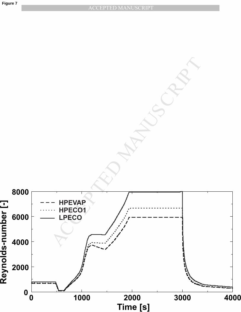
The averaged Reynolds-numbers for selected heating surfaces are pre-
sented in Fig. 7. The Re-numbers are averaged over the individual heat-
ing surface. It can be seen, that the curves for the Reynolds-numbers are
very close together during the periods with a low flue gas mass flow. A
higher flue gas mass flow and temperature leads to an expanding of the
Reynolds-numbers between the different heating surfaces. The heating sur-
31

faces located in the region with lower flue gas temperature leads to higher
Reynolds-numbers compared to the heating surfaces located in the region
with higher flue gas temperature. The highest values for Re are reached, of
course, under full operation conditions.
A comparison of the Reynolds-numbers with the range of validity of the
different heat transfer correlations used in this investigation shows, that the
calculated Re-numbers are located at the lower end or in case of a low GT
exhaust flue gas mass flow out of the definition region of the Nu-correlations.
But for the dynamic simulation of the start-up or shutdown behavior of a
boiler an extrapolation of the heat transfer correlations must be done. This is
based on the circumstance that the lower boundary for the definition region
of all heat transfer correlations, which are known by the authors, are too
high for Re→ 0.
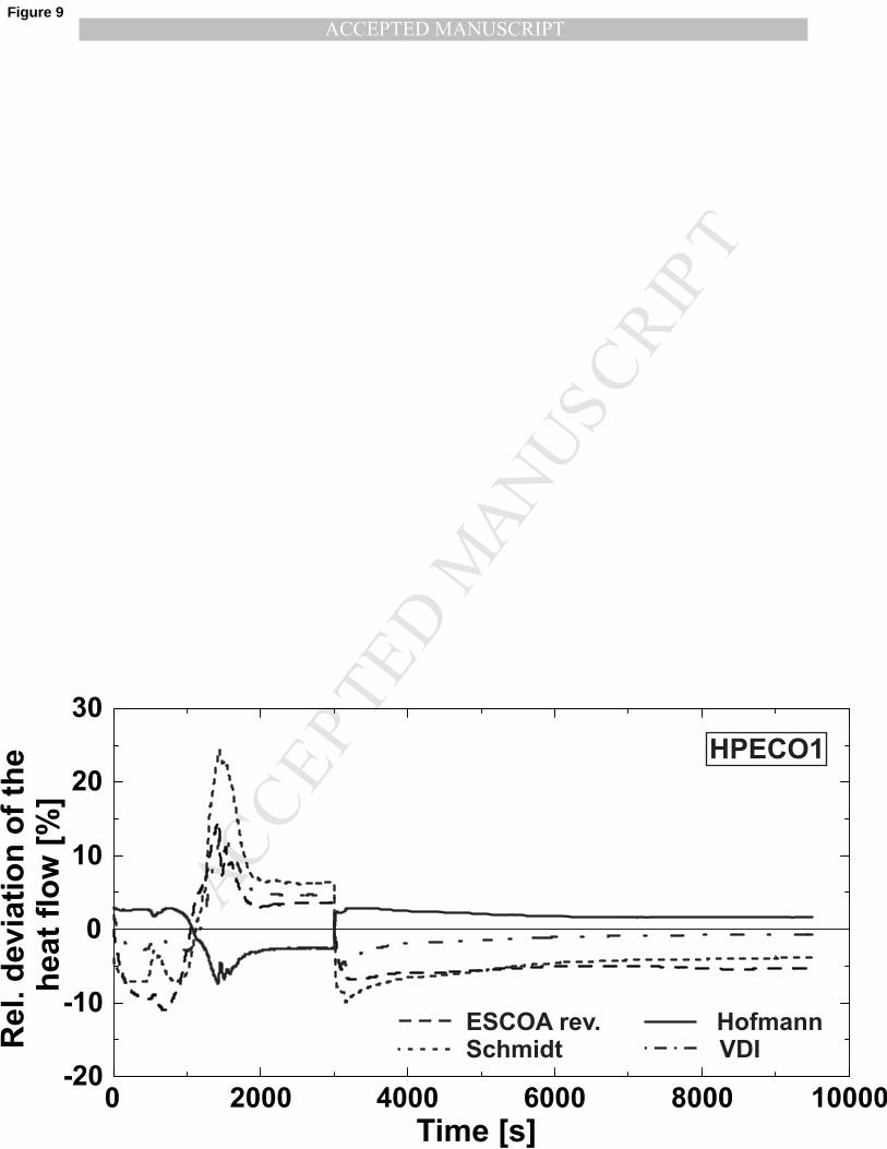
The heat flow from the flue gas to the HPECO1 for the different Nu-
correlations is shown in Fig. 8. Between the simulation time of 4000 and
9500 s the graphs in Fig. 8 grow together. The decrease of the absorbed
heat flow approx. 500 s after simulation start is a reaction to the decreasing
flue gas mass flow (synchronization of the gas turbine). The second decrease
in heat flow (at approx. 1500 s) is caused by the increase of the absorbed
heat in the HPEVAP and IPSH during this period. The figure shows clearly
that there are differences in the absorbed heat flows between the analyzed
correlations during the start-up and also at the full load period. The highest
variety of the heat flux compared to the traditional ESCOATM correlation
was given by the equation according to Schmidt. A more representative
presentation of this relationship can be seen with the help of the relative
32
deviation of the heat flow which is presented in Fig. 9.
All data used for Fig. 9 are referred to the traditional ESCOATM cor-
relation. The correlation according to Schmidt shows in the region around
full operation load of the boiler the highest values for the relative devia-
tion compared to the heat flow calculated with the traditional ESCOATM
correlation, while in the low Re-regions (see Fig. 7) the revised ESCOATM
correlation shows under the current simulation conditions the highest value
for Frel. The relative deviation of the correlation according to Hofmann is
less than 5% except a very small period during the second decrease period
of the absorbed heat flow. Under full operation load the correlations ac-
cording to Hofmann and also the revised ESCOATM correlation show the
lowest values for the relative derivation. The Nu-equation according to Hof-
mann underestimates while the revised ESCOATM correlation overestimates
the heat flow compared to the traditional ESCOATM correlation (see Fig.
8). The equation according to VDI represents the best agreement with the
traditional ESCOATM correlation at low Re-numbers. In this region all cor-
relations are out of their definition area and the heat transfer coefficient must
be extrapolated.
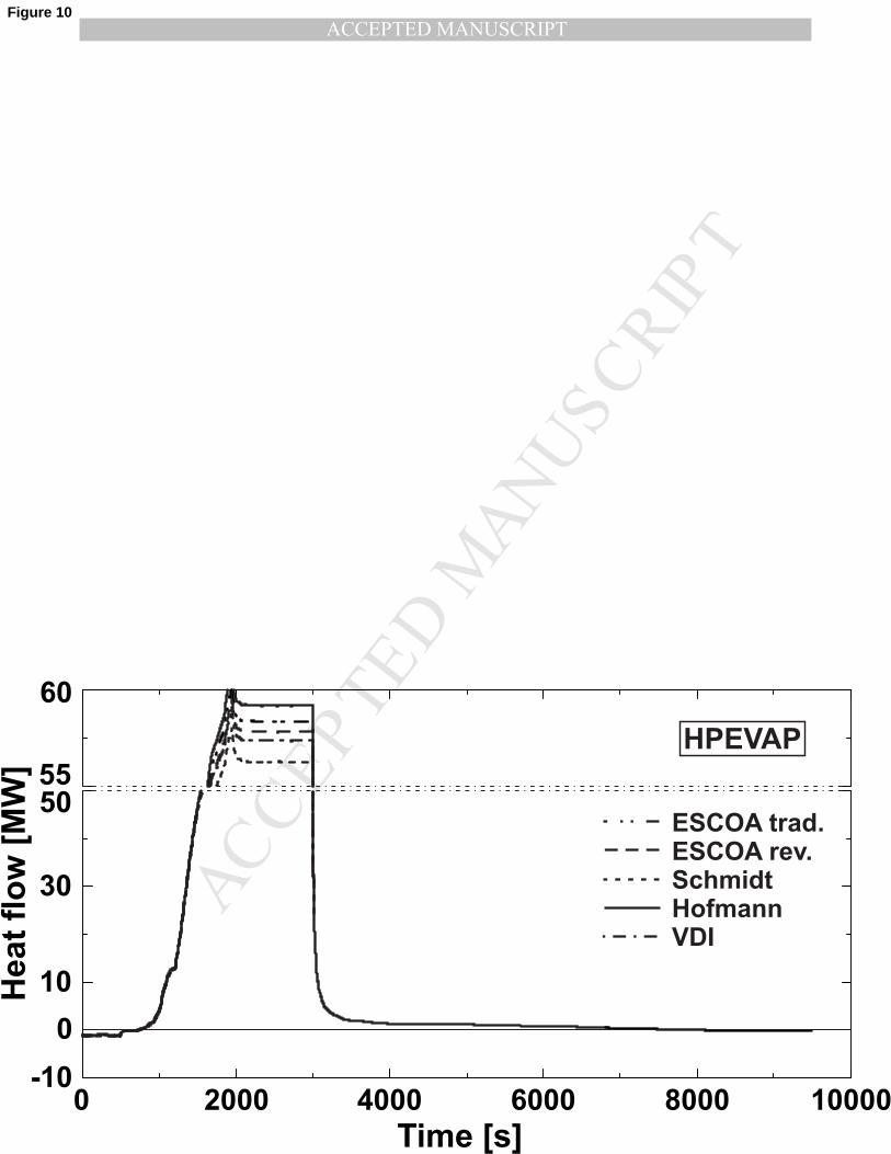
Figure 10 shows as a representative result of the numerical simulation
the absorbed heat flows of the HPEVAP, which is the heating surface with
the highest value of absorbed heat flow included in the HRSG. Every graph
in Fig. 10 represents the heat flow calculated with the help of one of the
Nusselt-correlations described in Section 3. It can be seen, that only under
full operation condition the absorbed heat flows differ among one another.
The highest difference is given with approx. 3 MW between the correlations
33
of Schmidt (lowest value) and Hofmann (highest value). This difference is
equivalent to approx. 1.7% of the total absorbed heat flow of the boiler at
full operation condition. This results also in a change of the overall circu-
lation ratio from 6 (Hofmann) to 6.3 (Schmidt). The curve according to
Hofmann as well as to the revised ESCOATM correlation are located close to
the traditional ESCOATM correlation also at full operation condition.
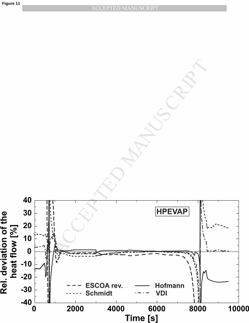
A view to the relative deviation of the absorbed heat flow of the HPEVAP,
which is presented in Fig. 11, show a small deviation to the traditional
ESCOATM equation. All investigated Nu-correlations show for Frel over a
wide range of the simulation a value smaller than 5%. The high deviation
from desired value of the traditional ESCOATM correlation at approx. 500
and 8000 s after simulation start is given by the circumstance that the heat
flow changes the flow direction from e. g. heating to cooling the flue gas
(see small sketch in Fig. 12). Therefore the heat flux is close to zero, which
results in high values by calculating the relative deviation. This can be seen
also in the first and last period of the numerical simulation. During this
period Frel shows also higher values.
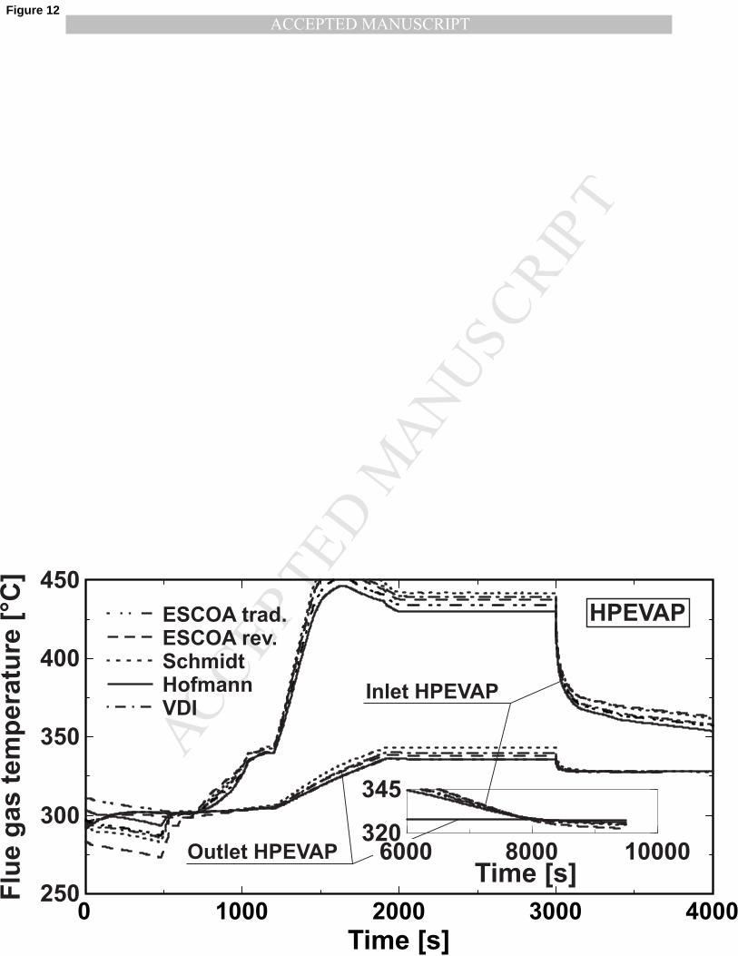
The development of the flue gas temperature over the time at the entrance
and at the exit of the HPEVAP of is shown in Fig. 12. During the first
approx. 600 s and the last period of the numerical simulation (> 8000 s, see
additional small sketch included in Fig. 12) the flue gas is heated up by the
HPEVAP. The graphs in Fig. 10 have shown that only under full operation
condition some differences in the heat flow is given between the different
correlations whereas the curves for the flue gas show also some variations
for the first approx. 600 s of simulation and during the GT shutdown. The
34
curves of the flue gas inlet temperature calculated with the different Nu-
correlations differ mostly at the first period of start-up. This results in a
variation of the downcomer mass flow in the HPEVAP which is presented in
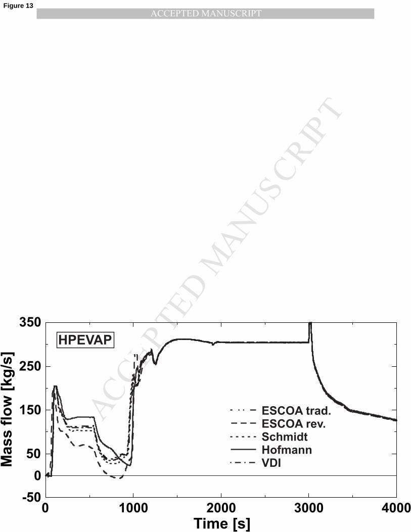
Fig. 13.
Figure 13 shows a comparison of the downcomer mass flow in the HPE-
VAP. It can be seen clearly, that the different evolution of the flue gas inlet
temperature at simulation start (< 600 s) results in a variation of the down-
comer mass flow. The curves which belongs to the correlations according to
Schmidt, VDI and ESCOATM traditional show approx. the same evolution
while the downcomer mass flow which belongs to Hofmann results to the
highest circulation mass flow during this period. The smallest downcomer
mass flow during this period is given by the revised ESCOATM correlation.
The calculation results with the revised ESCOATM correlation shows under
the analyzed operation conditions that between approx. 750 and 900 s after
start-up reverse flow of the fluid mass flow in the downcomer is possible.
This can lead under unfavorable operation conditions to a unstable behavior
(static instability like the Ledinegg instability) of the boiler, especially under
low operation pressure. Such a behavior for natural circulation boilers are
reported in the literature by e.g. [28, 1, 2, 3].
The above presented comparison are done from the view point of the
boiler behavior. In the following section the authors will give an explanation
of the results from the view point of the heat transfer correlation background.
The most important fact are the different temperatures of the tube bundle
heating surfaces, influencing the correlations of the dimensionless heat trans-
fer coefficients. As stated above, with a rising or decreasing temperature the
35
Re-number decreases or rises and thus different heat transfer coefficients are
evaluated. This can be seen in the general formulation of the heat transfer
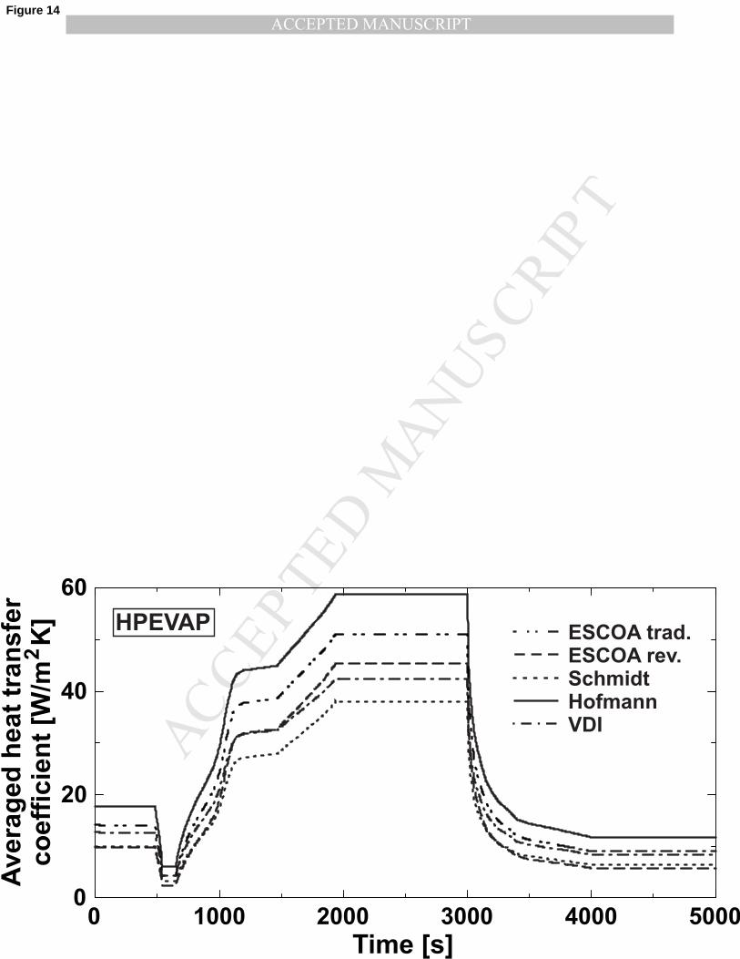
correlations presented above. A global comparison of the average heat trans-
fer coefficient at the HPEVAP, which is representative for all the heating
surfaces of the boiler, is depicted in Fig. 14. As seen, generally the lowest
heat transfer coefficients are evaluated with Schmidt’s correlation. This cor-
responds to the fact that these equations are evaluated mostly for annular
solid fins. The highest coefficients are found by the correlation of Hofmann.
This may be explained due to the exceed in range of validity partly of these
equations. A comparison of the heat transfer coefficients calculated by the
equations of ESCOATM traditional and VDI show a very small difference,
especially during start-up. In between Hofmann and ESCOATM revised the
traditional correlation of ESCOATM is located. It has to be noted that all
correlations according to their definition region are in general valid above
approx. 1000 s.
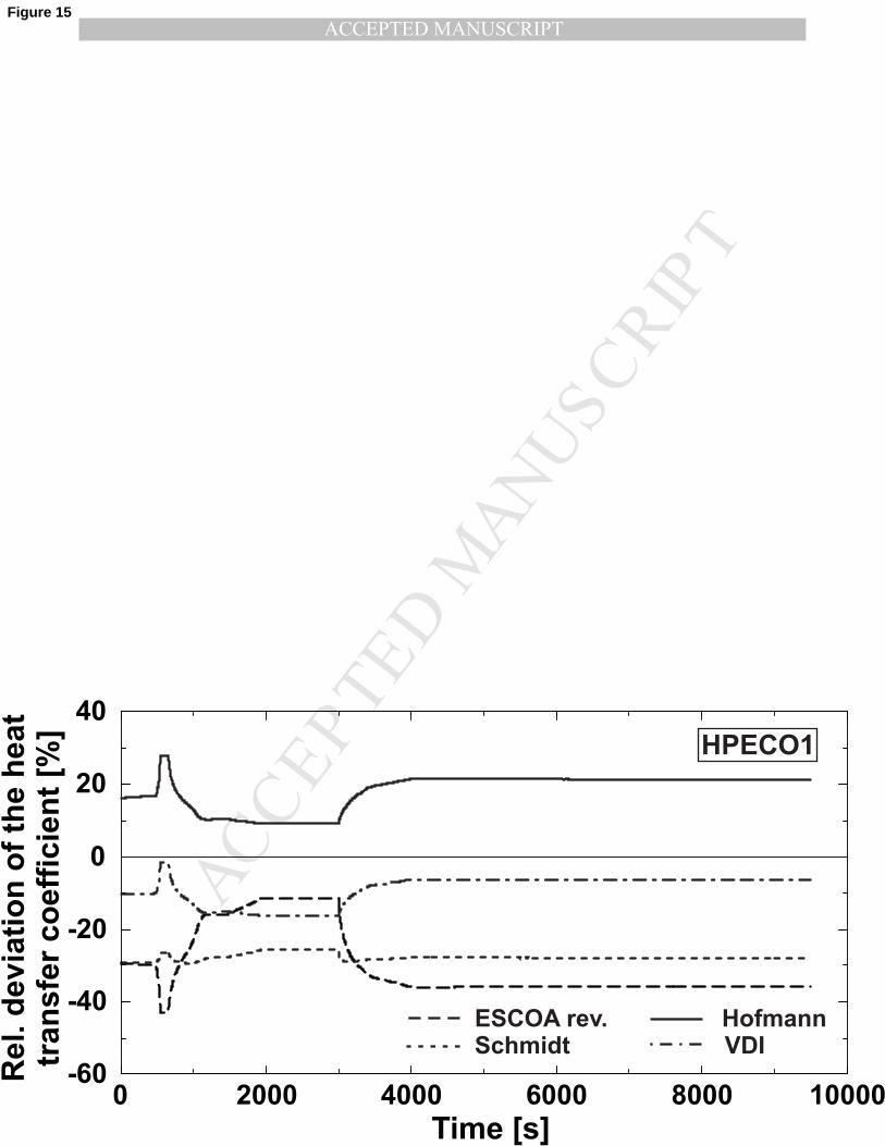
A detailed view into the tube bundle heating surfaces LPECO, HPE-
VAP, and HPECO1 will provide further information about the influence of
the different heat transfer correlations. Within the three compared heating
surfaces, the HPECO1 is located near the flue gas outlet, upstream of the
HPEVAP. Due to lower temperatures, the Re-numbers are in the range of
approx. 6800. In Fig. 15 the relative deviation of the heat transfer coeffi-
cients, based on the traditional ESCOATM correlations, is presented. During
start-up and shutdown the range of validity is exceeded. Thus a high varia-
tion of up to 40% can be ascerteained within all curves. In the range of the
stationary operation at full load a remarkable difference between Schmidt
36
and ESCOATM traditional of almost 30 % is noticed. All other equations
are located within 15% deviation. As also found in the global consideration,
both the ESCOATM revised and the VDI correlation has a good agreement.
Almost similar results are obtained within a comparison of the equations
at the HPEVAP. As a fact of the very close location of the heating surfaces
to the flue gas entry, the temperatures are very high. Due to high kinematic
viscosity, the evaluated Re-numbers are below 6000. At the lower Re-range of
all heat transfer correlations the deviation will increase, which may be seen in
the exponent of the Re-number, varying in between 0.6 to 0.75 (see Eq. (41)
to (50)). Thus different gradients within the functions are evaluated. A com-
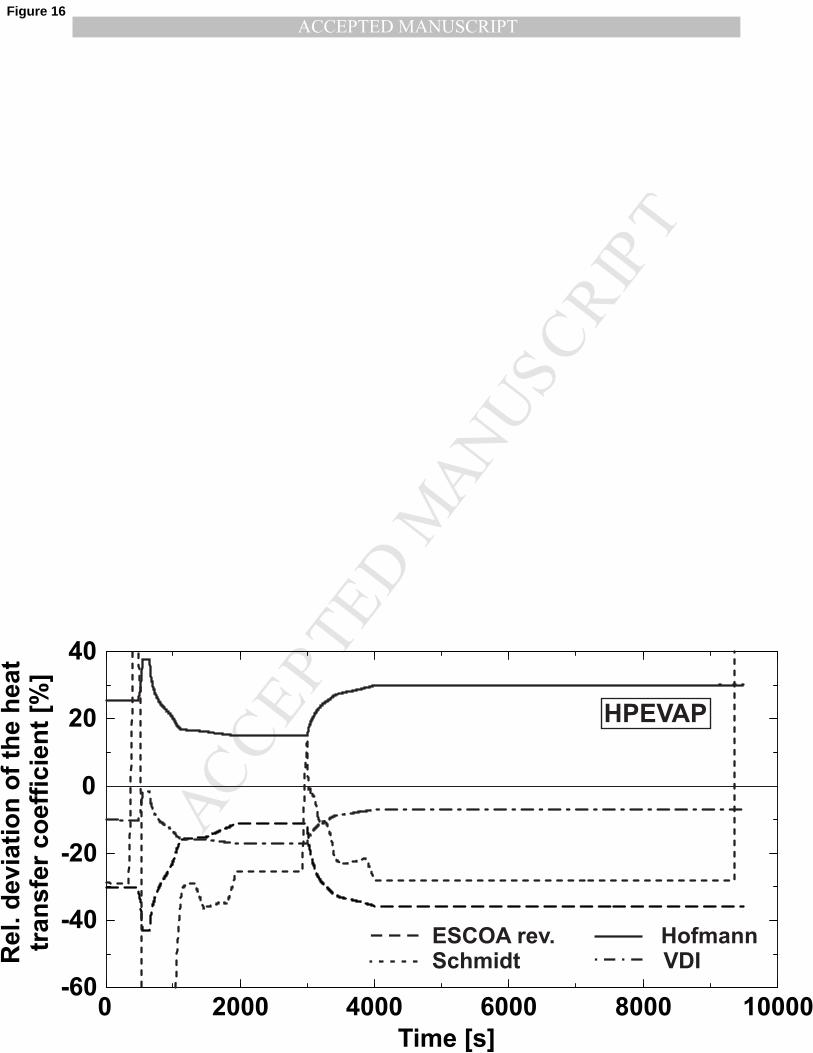
parison of Fig. 15 and 16 indicates almost same heat transfer progression but
with higher deviations. The differences may also be amplified by fact of dif-
ferent tube row numbers. Each individual author defines different reduction
coefficients for the heat transfer at fewer tube rows. But the most formulas
for calculating heat transfer at finned-tubes are generally valid for a certain
minimum number of consecutive tube rows and indicates a critical value of
equal or more than 8 rows in flow direction. At the HPECO1 5 consecutive
tube rows and at the HPEVAP 12 consecutive tube rows are installed. In
the range of the stationary operation the deviations of all correlations except
Schmidt varies in between 20%.
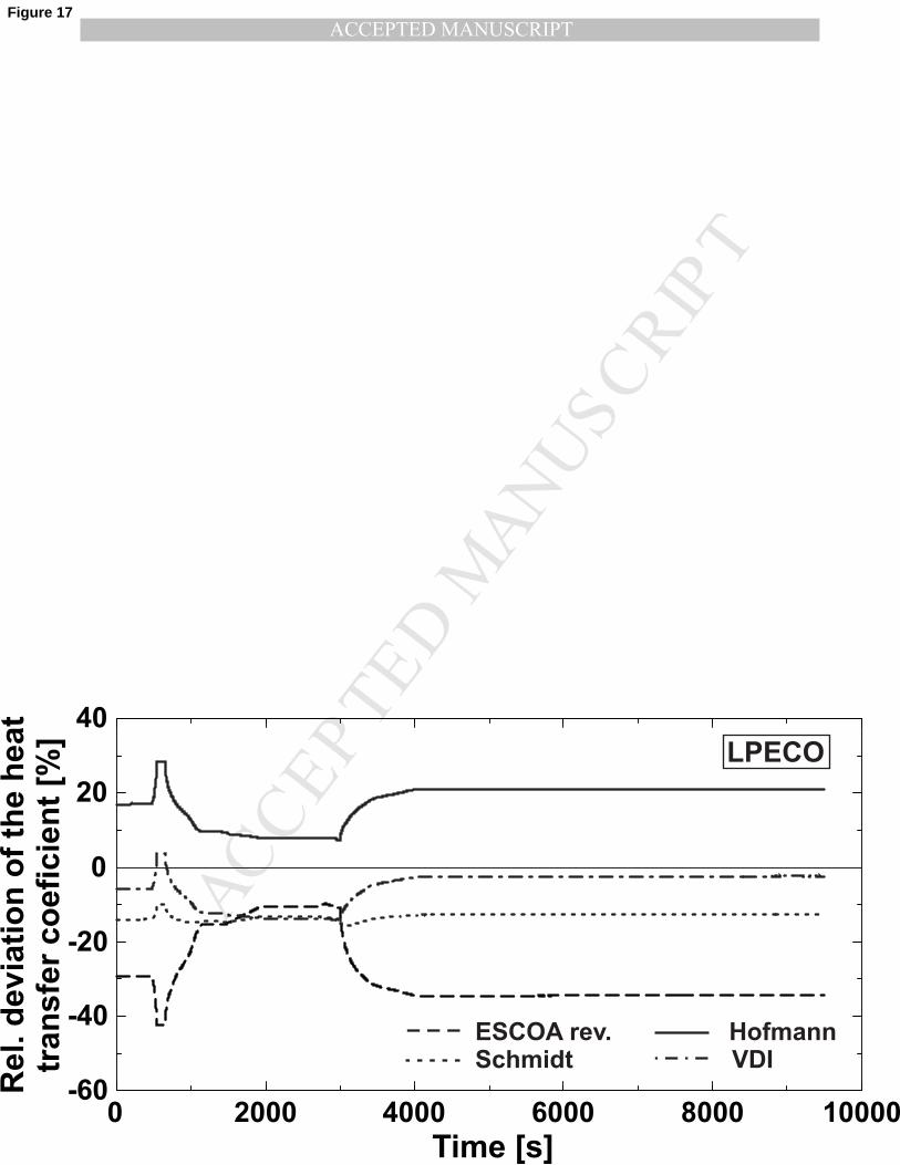
At the upper end of the flue gas pass through the HRSG the LPECO is
installed. Apart from low temperatures and thus higher Re-numbers (ap-
prox. 8000), the deviations are small (see Fig. 17). As seen in Fig. 14
and 17, the equation of Hofmann evaluates for generally higher heat trans-
fer coefficients, than equations of the authors in the comparison. All other
37
correlations are located very close together in between 2000 and 3000 s. The
LPECO is applied with two consecutive arranged tube rows, indicating also
any influences from tube arrangements. Depending on the longitudinal pitch
tl, the heat transfer coefficient differs for various tube bundle configurations.
Thus, different values of a reduction coefficient for a single tube row or two
consecutive arranged tube rows are obtained, compare values of e.g. [29] and
[24]. Considering this effect, Weierman [25] and ESCOATM in [6], stated
their reduction coefficient in dependence of tl/tt.
6. Conclusions
The influence of different Nu-correlations for finned-tubes, namely the
correlations according to Hofmann, ESCOATM traditional and revised, Schmidt
and VDI, on the dynamic behavior of a three stage HRSG under hot start-up
condition was studied theoretically. The study was done for a start-up and
shutdown sequence of a GT. Therefore the Re-number was in some parts of
the simulation out of the definition region of the different Nu-correlations
and must be extrapolated.
The investigation of the HRSG calculated with the different correlations
shows, that under the analyzed conditions the influence of the different cor-
relations on the overall behavior of the boiler is small. The total absorbed
heat flow of the boiler during the simulation was equal within small limits.
A further result of the analysis is, that the differences in the behavior of
the steam generator are given in the details. For the same heating surfaces
of the boiler the absorbed heat flow are different for the investigated corre-
lations. This results to different operation conditions in some parts of the
38
boiler during the start-up and shutdown process. In the worst case the boiler
can lead to unfavorable operation conditions, e.g. reverse flow or a change of
the flow direction in some parts of the evaporators. In such a case a redesign
of the boiler must be done. Therefore it is necessary to accomplish all cal-
culations with the tube related correlations, especially for detail analysis or
the design of the bundle heating surfaces.
A further result is obtained by a comparison of the heat transfer coeffi-
cient at different heating surfaces. It is indicated that the choice of different
correlations at the gas-side mass flow inlet and outlet influences the design
properties of the HRSG.
In the next step the numerical results should be verified by measured data
at a real power plant.
References
[1] H. Walter, W. Linzer, The influence of the operating pressure on the
stability of natural circulation systems, Applied Thermal Engineering
26 (7/8) (2006) 892–897.
[2] H. Walter, W. Linzer, Flow Stability of Heat Recovery Steam Genera-
tors, Trans. of ASME, Ser. D, Journal of Engineering for Gas Turbines
and Power 128 (2006) 840–848.
[3] A. Stribersky, W. Linzer, Ein Beitrag zum Problem der Stabilitaet beim
Naturumlauf, Fortschr.-Ber. VDI 154, VDI Verlag, Duesseldorf (1984).
[4] T. E. Schmidt, Der Waermeuebergang an Rippenrohre und die Berech-
39
nung von Rohrbuendel-Waermeaustauschern, Kaeltetechnik 15 (4)
(1963) 98–102.
[5] VDI-Heat Atlas, 10th Edition, Springer-Verlag, Berlin Heidelberg New
York, 2006.
[6] V. Ganapathy, Industrial Boilers and Heat Recovery Steam Generators,
Marcel Dekker Inc., New York Basel, 2003.
[7] ESCOA, Turb-X HF and Soldfin HF Rating Instructions, ESCOA,
Pryor, Oklahoma (1979).
[8] R. Hofmann, F. Frasz, K. Ponweiser, Experimental Heat Transfer Inves-
tigation of Tube Row Effects at Air Side Heat Exchanger with Serrated
Finned-Tubes, in: Proceedings of the 6th IASME/WSEAS International
Conference on Heat Transfer, Thermal Engineering and Environment,
2008, pp. 193–201.
[9] R. Hofmann, Experimental and Numerical Gas-Side Performance Evalu-
ation of Finned-Tube Heat Exchangers, Dissertation, Vienna University
of Technology (2009).
[10] H. Walter, Modellbildung und numerische Simulation von Naturum-
laufdampferzeugern, Fortschr.-Ber. VDI 457, VDI Verlag, Duesseldorf
(2001).
[11] H. Walter, Dynamic simulation of natural circulation steam generators
with the use of finite-volume-algorithms – A comparison of four algo-
rithms, Simulation Modelling Practice and Theory 15 (2007) 565–588.
40
[12] S. V. Patankar, Numerical Heat Transfer and Fluid Flow, Series in Com-
putational Methods in Mechanics and Thermal Sciences, Hemisphere
Publ. Corp., Washington, New York, London, 1980.
[13] L. Friedel, Improved Friction Pressure Drop Correlations for Horizon-
tal and Vertical Two-Phase Pipe Flow, in: European Two Phase Flow
Group Meeting, Ispra, Italien, 1979, pp. 1–25.
[14] H. Richter, Rohrhydraulik, 4th Edition, Springer Verlag, Berlin, Heidel-
berg, 1962.
[15] E. Fried, I. E. Idelchik, Flow Resistance: A Design Guide for Engineers,
Hemisphere Publishing Corporation, New York, Washington, Philadel-
phia, London, 1989.
[16] H. Walter, W. Linzer, Numerical Simulation of a Three Stage Natural
Circulation Heat Recovery Steam Generator, IASME Transactions 2 (8)
(2005) 1343–1349.
[17] B. Epple, R. Leithner, W. Linzer, H. Walter, Simulation von
Kraftwerken und waermetechnischen Anlagen, Springer Verlag, Wien,
2009.
[18] L. Haar, J. S. Gallagher, G. S. Kell, NBS/NRC Wasserdampftafeln,
Springer-Verlag, Berlin, 1988.
[19] F. Brandt, Dampferzeuger: Kesselsysteme, Energiebilanz, Stroemung-
stechnik, 2nd Edition, Vol. 3 of FDBR - Fachbuchreihe, Vulkan-Verlag,
Essen, 1999.
41
[20] F. Richter, Physikalische Eigenschaften von Staehlen und ihre Tem-
peraturabhaengigkeit, MANNESMANN Forschungsberichte 10, Verlag
Stahleisen m. b. H., Duesseldorf (1983).
[21] R. Hofmann, F. Frasz, K. Ponweiser, Heat Transfer and Pressure Drop
Performance Comparison of Finned-Tube Bundles in Forced Convection,
WSEAS-Transactions on Heat and Mass Transfer 2 (4) (2007) 72–88.
[22] J. Tenner, P. Klaus, S. E., Erfahrungen bei der Erstellung und dem
Einsatz eines Datenvalidierungsmodells zur Prozessueberwachung und
-optimierung im Kernkraftwerk Isar 2, VGB Kraftwerkstechnik 4 (1998)
43–49.
[23] DIN 1319, Grundlagen der Messtechnik, Tech. rep., DIN, Berlin, Part 1
to 4 (1996).
[24] F. Frasz, L. W., Waermeuebergangsprobleme an querangestroemten
Rippenrohrbuendeln, BWK 44 (7/8) (1992) 333–336.
[25] C. Weierman, Correlations Ease the Selection of Finned Tubes, The Oil
and Gas Journal 74 (36) (1976) 94–100.
[26] F. Frasz, Principles of Finned-Tube Heat Exchanger Design for En-
hanced Heat Transfer, Heat and Mass Transfer, WSEAS-Press, 2008,
edited by Hofmann, R. and Ponweiser, K.
[27] R. Leithner, Vergleich zwischen Zwangdurchlaufdampferzeuger, Zwang-
durchlaufdampferzeuger mit Vollastumwaelzung und Naturumlauf-
dampferzeuger, VGB Kraftwerkstechnik 63 (7) (1983) 553–568.
42
[28] H. Walter, Theoretical Stability Analysis of a Natural Circulation Two-
Pass Steam Generator: Influence of the Heating Profile and Operation
Pressure, WSEAS Transactions on Heat and Mass Transfer 1 (3) (2006)
274–282.
[29] J. Stasiulevicius, A. Skrinska, Heat Transfer of Finned Tube Bundles
in Crossflow, Hemisphere Publ. Corp., Washington New York London,
1988, edited by Zukauskas, A. and Hewitt, G.
43

List of Figure Captions
1. Figure 1: Discretization of the header and the header connected tubes
2. Figure 2: Sectional sketch of the investigated finned-tube with U/I-
shape
3. Figure 3: Sketch of the bundle heating surfaces arrangement of the
HRSG boiler
4. Figure 4: Gas turbine exhaust flue gas mass flow and temperature
5. Figure 5: Flue gas temperature at selected points in the flue gas pass
of the boiler
6. Figure 6: Mass flow in the downcomer and at the outlet of the highest
heated tube path of the different evaporators
7. Figure 7: Averaged Re-numbers of selected bundle heating surfaces
8. Figure 8: Heat flow from the flue gas to HPECO1
9. Figure 9: Relative deviation of the absorbed heat flow of HPECO1
10. Figure 10: Heat flow from the flue gas to HPEVAP
11. Figure 11: Relative deviation of the absorbed heat flow of HPEVAP
12. Figure 12: Flue gas temperature at the inlet and outlet of HPEVAP
13. Figure 13: Mass flow in the downcomer of HPEVAP
14. Figure 14: Average heat transfer coefficient at the HPEVAP
15. Figure 15: Relative deviation of the heat transfer coefficient at the
HPECO1
16. Figure 16: Relative deviation of the heat transfer coefficient at the
HPEVAP
44

17. Figure 17: Relative deviation of the heat transfer coefficient at the
LPECO
45

List of Table Captions
1. Table 1: Specifications of investigated finned-tubes
2. Table 2: Geometric data of the HRSG boiler
46
Table 1:
Fin Geometry Notation U-shaped I-shaped
segmented segmented
Bare tube diameter da 38.0 mm 38.0 mm
Tube thickness s 3.2 mm 4.0 mm
Number of fins per m Nf 295 276
Average fin height H 20.0 mm 15.5 mm
Average fin thickness sf 0.8 mm 1.0 mm
Average tube length L 495 mm 500 mm
Average segment width bs 4.3 mm 4.5 mm
Number of tubes in flow-direction Nr 8, 6, 4, 2, 1 8, 4, 2
Number of tubes per row NL 11 1
Longitudinal tube pitch tl 79 mm 9 mm
Transversal tube pitch tt 85 mm 5 mm
Outside surface area for 8 tube rows Atot 84.48 m2 64.05 m2
Fin material DC01 St 37.2
Tube material St 35.8 St 35.8
Net free area of tube row Amin 0.2292 m2 0.2326 m2
45
Table(s)
Table 2:
Name of Number Number of Number of Fin
the heating of tube parallel tubes fins per hight
surface layers per layer m tube [mm]
HPECON5 12 74 275 17
HPECON4 5 74 275 17
HPECON3 9 74 275 17
HPECON2 5 74 275 17
HPECON1 5 84 275 17
HPEVAP 12 84 268 17
HPSH1 3 84 128 11
HPSH2 4 84 272 11
IPECO1 2 84 268 17
IPEVAP 6 84 257 17
IPSH 2 84 110 17
LPECO 2 84 268 17
LPEVAP 6 84 270 17
46
Table(s)
1,k
0+1/
2,k0+1/2,k+1
1+1/2,k+1
2+1/2,k+1
3,k+1
2,k+1
1,k+1
1+1/
2,k
2+1/
2,k
2,k
3,k
h
i,j
i-1,j
i-1/2,j
i-3/2,j
i-2,j
i+1/2,j
Figure 1
Helical U-finsHelical I-fins
Contactarea
Contactarea
t fsfbs
Hs
s
da
D
H
Figure 2
HPECON1
HPECON4
HPECON3
HPECON2
HPEVAP
HPSH1
HPSH2
LPECONLP-drum
IP-drum
HP-drum
LPEVAP
IPEVAP
IPSH
IPECON
Flu
eg
as
Figure 3
0 1000 2000 3000 4000
Time [s]
0
200
400
600
Flu
e g
as t
em
pera
ture
[°C
]F
lue g
as m
ass f
low
[kg
/s]
Temperature
Mass flow
Figure 4

0 2000 4000 6000 8000 10000
Time [s]
0
200
400
600
Flu
e g
as t
em
pera
ture
[°C
]
Gas turbine outlet
Inlet HPEVAP
Inlet LPEVAP
Inlet IPEVAP
Figure 5
0
0
2000 4000 6000 8000 10000
Time [s]
-50
50
150
250
350
Mass f
low
[kg
/]
Downcomer
Outlet hotest tube path evaporator
HP-SystemIP-SystemLP-System
Figure 6
0
2000
4000
6000
8000
Re
yn
old
s-n
um
be
r [-
] HPEVAPHPECO1LPECO
0 1000 2000 3000 4000
Time [s]
Figure 7

0 1000 2000 3000 4000
Time [s]
0
2
4
6
8
He
at
flo
w [
MW
]
ESCOA trad.
SchmidtHofmannVDI
ESCOA rev.
HPECO1
Figure 8
0 2000 4000 6000 8000 10000
Time [s]
-20
-10
0
10
20
30
Re
l. d
ev
iati
on
of
the
he
at
flo
w [
%]
ESCOA rev. HofmannSchmidt VDI
HPECO1
Figure 9
0
0
2000 4000 6000 8000 10000
Time [s]
-10
10
30
50
Heat
flo
w [
MW
]
ESCOA trad.
SchmidtHofmannVDI
ESCOA rev.
55
60
HPEVAP
Figure 10
Rel. d
evia
tio
n o
f th
eh
eat
flo
w [
%]
ESCOA rev. HofmannSchmidt VDI
HPEVAP
0 2000 4000 6000 8000 10000
Time [s]
-40
-30
-20
-10
0
10
20
30
40
Figure 11
250
300
350
400
450
Flu
e g
as
te
mp
era
ture
[°C
]
ESCOA trad.
SchmidtHofmannVDI
ESCOA rev.
HPEVAP
Inlet HPEVAP
Outlet HPEVAP 6000 8000 10000Time [s]
320
345
0 1000 2000 3000 4000
Time [s]
Figure 12
0
0
1000 2000 3000 4000
Time [s]
-50
50
150
250
350
Ma
ss
flo
w [
kg
/s]
HPEVAP
ESCOA trad.
SchmidtHofmannVDI
ESCOA rev.
Figure 13
0 1000 2000 3000 4000 5000
Time [s]
0
20
40
60
Avera
ged
heat
tran
sfe
rco
eff
icie
nt
[W/m
K
]2
ESCOA trad.
SchmidtHofmannVDI
ESCOA rev.
HPEVAP
Figure 14
0 2000 4000 6000 8000 10000
Time [s]
-60
-40
-20
0
20
40
Rel. d
evia
tio
n o
f th
e h
eat
tran
sfe
r co
eff
icie
nt
[%]
ESCOA rev. HofmannSchmidt VDI
HPECO1
Figure 15
0 2000 4000 6000 8000 10000
Time [s]
-60
-40
-20
0
20
40
Rel. d
evia
tio
n o
f th
e h
eat
tran
sfe
r co
eff
icie
nt
[%]
ESCOA rev. HofmannSchmidt VDI
HPEVAP
Figure 16
0 2000 4000 6000 8000 10000
Time [s]
-60
-40
-20
0
20
40
Rel. d
evia
tio
n o
f th
e h
eat
tran
sfe
r co
efi
cie
nt
[%]
ESCOA rev. HofmannSchmidt VDI
LPECO
Figure 17