how is project #1 going? - pdfs.semanticscholar.org filewhy is this hard? simple analogy: 11 is the...

How is project #1 going?

Edge Detection

Last Lecture

Filtering

Pyramid

Today

Motion Deblur

Image Transformation

Removing Camera Shake from a Single Photograph

Rob Fergus, Barun Singh, Aaron Hertzmann, Sam T. Roweis and William T. Freeman

Massachusetts Institute of Technology and

University of Toronto

http://people.csail.mit.edu/fergus/research/deblur.html

Overview

Original Our algorithm

Close-up

Original Naïve Sharpening Our algorithm

Let’s take a photo

Blurry result

Slow-motion replay

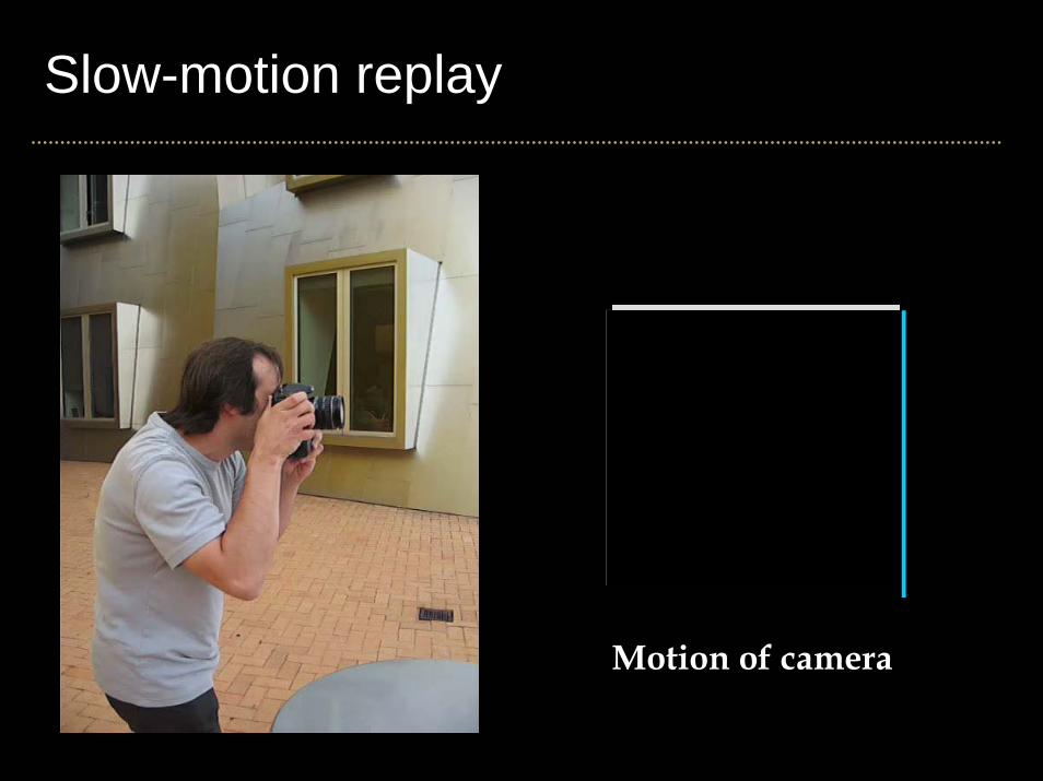
Slow-motion replay

Motion of camera

Image formation process

= ⊗

Blurry image Sharp image

Blur kernel

Input to algorithm Desired outputConvolution

operatorModel is approximation

Why is this hard?

Simple analogy:11 is the product of two numbers.What are they?

No unique solution: 11 = 1 x 1111 = 2 x 5.511 = 3 x 3.667 etc…..

Need more information !!!!

Multiple possible solutions

= ⊗

Blurry image

Sharp image Blur kernel

= ⊗

= ⊗

Natural image statistics

Histogram of image gradients

Characteristic distribution with heavy tails

Blury images have different statistics


Parametric distribution


Use parametric model of sharp image statistics

Three sources of information1. Reconstruction constraint:

=⊗

Input blurry imageEstimated sharp imageEstimatedblur kernel

2. Image prior: 3. Blur prior:Positive

&Sparse

Distribution of gradients

Variational Bayesian method

Based on work of Miskin & Mackay 2000

Keeps track of uncertainty in estimates of image and blur by using a distribution instead of a single estimate

Helps avoid local maxima and over-fitting

VariationalBayes

Variational Bayesian method

Maximum a-Posteriori (MAP)

Pixel intensity

Scor

e

Objective function for a single variable

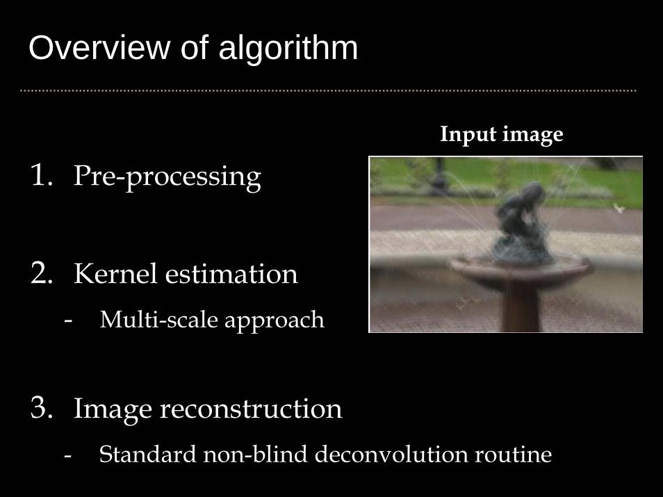
Overview of algorithm

Input image

1. Pre-processing

2. Kernel estimation- Multi-scale approach

3. Image reconstruction- Standard non-blind deconvolution routine

Preprocessing

Convert tograyscale

Input image

Remove gammacorrection

User selects patchfrom image

Bayesian inference too slow to run on whole image

Infer kernel from this patch

InitializationInput image

Initialize 3x3 blur kernel

Initial blur kernelBlurry patch Initial image estimate

Convert tograyscale



Inferring the kernel: multiscale methodInput image

Loop over scales

VariationalBayes

Upsampleestimates

Use multi-scale approach to avoid local minima:


Convert tograyscale



Image ReconstructionInput image

Full resolutionblur estimate

Non-blind deconvolution

(Richardson-Lucy)

Deblurredimage

Loop over scales

VariationalBayes

Upsampleestimates


Convert tograyscale



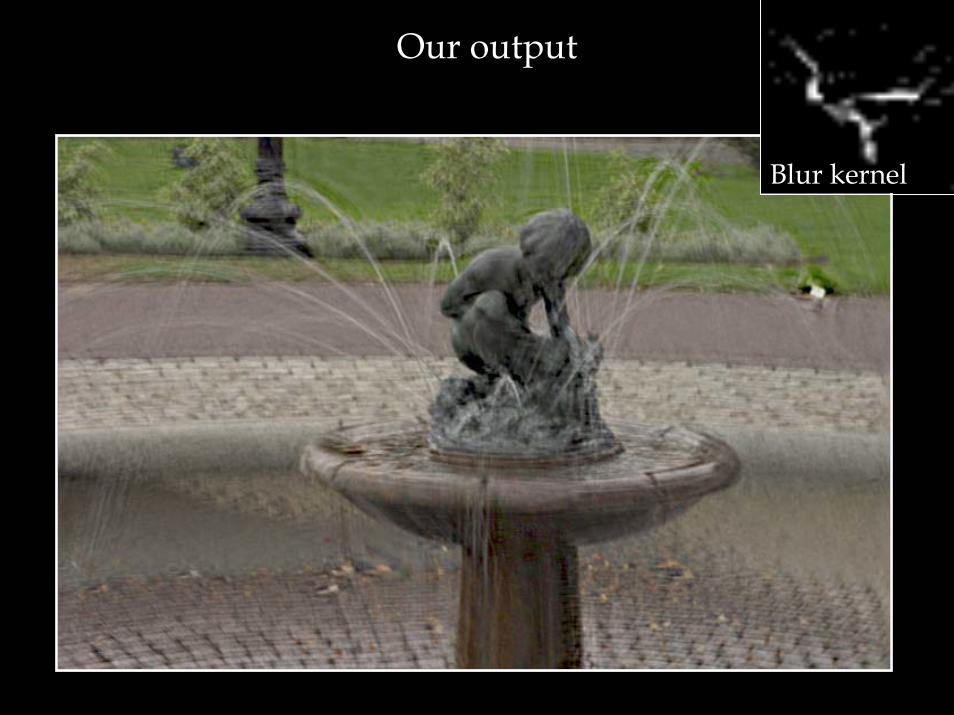
Results on real images

Submitted by people from their own photo collections

Type of camera unknown

Output does contain artifacts– Increased noise

– Ringing

Compares well to existing methods

Original photograph

Blur kernel Our output

Original photographMatlab’s deconvblind

Original photograph

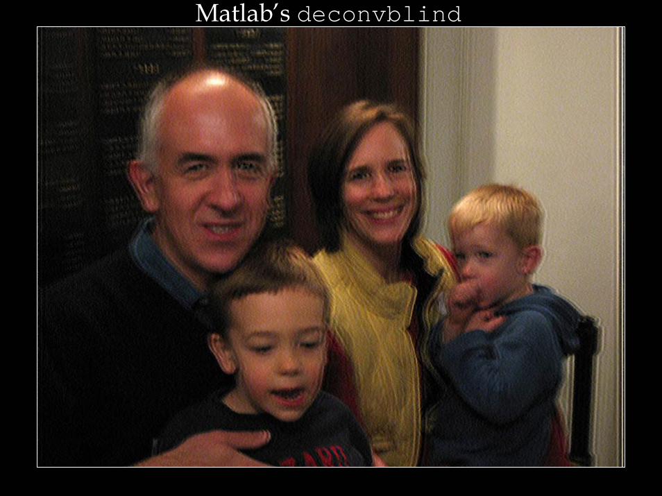
Matlab’s deconvblind

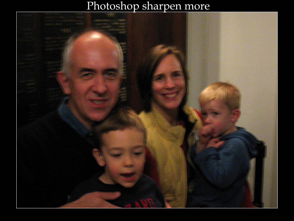
Photoshop sharpen more

2 4 6 8 10 12

2

4

6

8

Our output Blur kernel

2 4 6 8 10 12

2

4

6

8

Original photograph

1

2

3

4

5

6

7

8

9

Our output

Blur kernel

Original photograph

Our output

Blur kernel

Matlab’s deconvblind

Original photograph

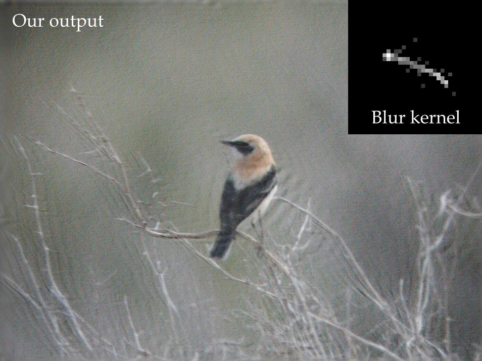
Our output

Blur kernel

Close-up of bird

Original Our output

Original photograph

Our output

Blur kernel

Image artifacts & estimated kernels

Blur kernels

Image patternsNote: blur kernels were inferred from large image patches,

NOT the image patterns shown

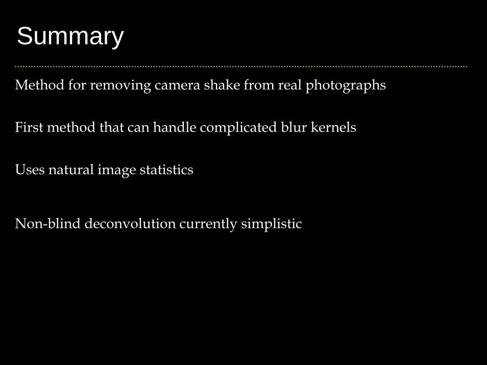
Summary

Method for removing camera shake from real photographs

First method that can handle complicated blur kernels

Uses natural image statistics

Non-blind deconvolution currently simplistic

Image Warping

• image filtering: change range of image• g(x) = T(f(x))

f

x

Tf

x

f

x

Tf

x

• image warping: change domain of image• g(x) = f(T(x))

Image Warping

• image filtering: change range of image• g(x) = T(f(x))

T

T

• image warping: change domain of image• g(x) = f(T(x))

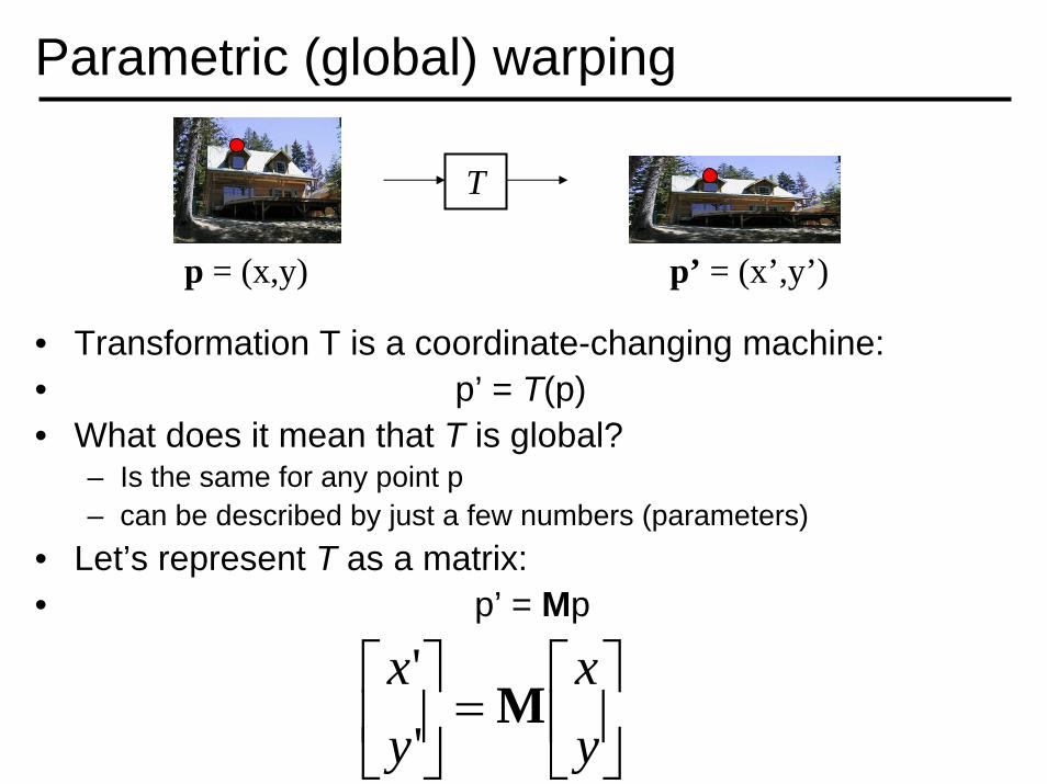
Parametric (global) warping

• Examples of parametric warps:

translation rotation aspect

affineperspective

cylindrical

Parametric (global) warping

• Transformation T is a coordinate-changing machine:• p’ = T(p)• What does it mean that T is global?

– Is the same for any point p– can be described by just a few numbers (parameters)

• Let’s represent T as a matrix:• p’ = Mp

T

p = (x,y) p’ = (x’,y’)

⎥⎦

⎤⎢⎣

⎡=⎥

⎦

⎤⎢⎣

⎡yx

yx

M''

Scaling

• Scaling a coordinate means multiplying each of its components by a scalar

• Uniform scaling means this scalar is the same for all components:

× 2

• Non-uniform scaling: different scalars per component:

Scaling

X × 2,Y × 0.5

Scaling

• Scaling operation:

• Or, in matrix form:

byyaxx

==''

⎥⎦

⎤⎢⎣

⎡⎥⎦

⎤⎢⎣

⎡=⎥

⎦

⎤⎢⎣

⎡yx

ba

yx

00

''

scaling matrix SWhat’s inverse of S?

2-D Rotation

θ

(x, y)

(x’, y’)

x’ = x cos(θ) - y sin(θ)y’ = x sin(θ) + y cos(θ)

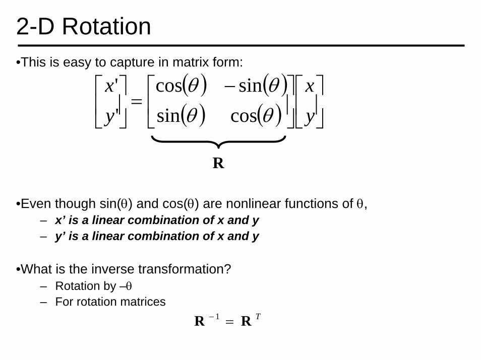
2-D Rotation•This is easy to capture in matrix form:

•Even though sin(θ) and cos(θ) are nonlinear functions of θ,– x’ is a linear combination of x and y– y’ is a linear combination of x and y

•What is the inverse transformation?– Rotation by –θ– For rotation matrices

( ) ( )( ) ( ) ⎥

⎦

⎤⎢⎣

⎡⎥⎦

⎤⎢⎣

⎡ −=⎥

⎦

⎤⎢⎣

⎡yx

yx

θθθθ

cossinsincos

''

TRR =− 1

R

2x2 Matrices

• What types of transformations can be represented with a 2x2 matrix?

2D Identity?

yyxx

==''

⎥⎦⎤

⎢⎣⎡⎥⎦⎤

⎢⎣⎡=⎥⎦

⎤⎢⎣⎡

yx

yx

1001

''

2D Scale around (0,0)?

ysy

xsx

y

x

*'

*'

=

=⎥⎦

⎤⎢⎣

⎡⎥⎦

⎤⎢⎣

⎡=⎥

⎦

⎤⎢⎣

⎡yx

ss

yx

y

x

00

''

2x2 Matrices


2D Rotate around (0,0)?

yxyyxx

*cos*sin'*sin*cos'

Θ+Θ=Θ−Θ=

⎥⎦

⎤⎢⎣

⎡⎥⎦

⎤⎢⎣

⎡ΘΘΘ−Θ

=⎥⎦

⎤⎢⎣

⎡yx

yx

cossinsincos

''

2D Shear?

yxshyyshxx

y

x

+=+=

*'*'

⎥⎦

⎤⎢⎣

⎡⎥⎦

⎤⎢⎣

⎡=⎥

⎦

⎤⎢⎣

⎡yx

shsh

yx

y

x

11

''

2x2 Matrices


2D Mirror about Y axis?

yyxx

=−=

''

⎥⎦⎤

⎢⎣⎡⎥⎦⎤

⎢⎣⎡−=⎥⎦

⎤⎢⎣⎡

yx

yx

1001

''

2D Mirror over (0,0)?

yyxx

−=−=

''

⎥⎦⎤

⎢⎣⎡⎥⎦⎤

⎢⎣⎡

−−=⎥⎦

⎤⎢⎣⎡

yx

yx

1001

''

2x2 Matrices


2D Translation?

y

x

tyytxx

+=+=

''

Only linear 2D transformations can be represented with a 2x2 matrix

NO!

All 2D Linear Transformations

• Linear transformations are combinations of …– Scale,– Rotation,– Shear, and– Mirror

• Properties of linear transformations:– Origin maps to origin– Lines map to lines– Parallel lines remain parallel– Ratios are preserved– Closed under composition

⎥⎦

⎤⎢⎣

⎡⎥⎦

⎤⎢⎣

⎡=⎥

⎦

⎤⎢⎣

⎡yx

dcba

yx''

⎥⎦⎤

⎢⎣⎡⎥⎦⎤

⎢⎣⎡⎥⎦⎤

⎢⎣⎡⎥⎦⎤

⎢⎣⎡=⎥⎦

⎤⎢⎣⎡

yx

lkji

hgfe

dcba

yx

''

Homogeneous Coordinates

• Q: How can we represent translation as a 3x3 matrix?

y

x

tyytxx

+=+=

''


•Homogeneous coordinates– represent coordinates in 2 dimensions with a 3-vector

⎥⎥⎥

⎦

⎤

⎢⎢⎢

⎣

⎡⎯→⎯⎥

⎦

⎤⎢⎣

⎡

1yx

yx


• Q: How can we represent translation as a 3x3 matrix?

• A: Using the rightmost column:

⎥⎥⎥

⎦

⎤

⎢⎢⎢

⎣

⎡

=100

1001

y

x

tt

ranslationT

y

x

tyytxx

+=+=

''

Translation

•Example of translation

⎥⎥⎥

⎦

⎤

⎢⎢⎢

⎣

⎡++

=⎥⎥⎥

⎦

⎤

⎢⎢⎢

⎣

⎡

⎥⎥⎥

⎦

⎤

⎢⎢⎢

⎣

⎡

=⎥⎥⎥

⎦

⎤

⎢⎢⎢

⎣

⎡

111001001

1''

y

x

y

x

tytx

yx

tt

yx

tx = 2ty = 1



• Add a 3rd coordinate to every 2D point– (x, y, w) represents a point at location (x/w, y/w)– (x, y, 0) represents a point at infinity– (0, 0, 0) is not allowed

Convenient coordinate system to represent many useful transformations

1 2

1

2 (2,1,1) or (4,2,2) or (6,3,3)

x

y

Basic 2D Transformations

• Basic 2D transformations as 3x3 matrices

⎥⎥⎥

⎦

⎤

⎢⎢⎢

⎣

⎡

⎥⎥⎥

⎦

⎤

⎢⎢⎢

⎣

⎡ΘΘΘ−Θ

=⎥⎥⎥

⎦

⎤

⎢⎢⎢

⎣

⎡

11000cossin0sincos

1''

yx

yx

⎥⎥⎥

⎦

⎤

⎢⎢⎢

⎣

⎡

⎥⎥⎥

⎦

⎤

⎢⎢⎢

⎣

⎡=

⎥⎥⎥

⎦

⎤

⎢⎢⎢

⎣

⎡

11001001

1''

yx

tt

yx

y

x

⎥⎥⎥

⎦

⎤

⎢⎢⎢

⎣

⎡

⎥⎥⎥

⎦

⎤

⎢⎢⎢

⎣

⎡=

⎥⎥⎥

⎦

⎤

⎢⎢⎢

⎣

⎡

11000101

1''

yx

shsh

yx

y

x

Translate

Rotate Shear

⎥⎥⎥

⎦

⎤

⎢⎢⎢

⎣

⎡

⎥⎥⎥

⎦

⎤

⎢⎢⎢

⎣

⎡=

⎥⎥⎥

⎦

⎤

⎢⎢⎢

⎣

⎡

11000000

1''

yx

ss

yx

y

x

Scale

Affine Transformations

• Affine transformations are combinations of …– Linear transformations, and– Translations

• Properties of affine transformations:– Origin does not necessarily map to origin– Lines map to lines– Parallel lines remain parallel– Ratios are preserved– Closed under composition

⎥⎥⎦

⎤

⎢⎢⎣

⎡

⎥⎥⎦

⎤

⎢⎢⎣

⎡=

⎥⎥⎦

⎤

⎢⎢⎣

⎡

wyx

fedcba

wyx

100''

Projective Transformations

• Projective transformations …– Affine transformations, and– Projective warps

• Properties of projective transformations:– Origin does not necessarily map to origin– Lines map to lines– Parallel lines do not necessarily remain parallel– Ratios are not preserved– Closed under composition

⎥⎥⎦

⎤

⎢⎢⎣

⎡

⎥⎥⎦

⎤

⎢⎢⎣

⎡=

⎥⎥⎦

⎤

⎢⎢⎣

⎡

wyx

ihgfedcba

wyx

'''

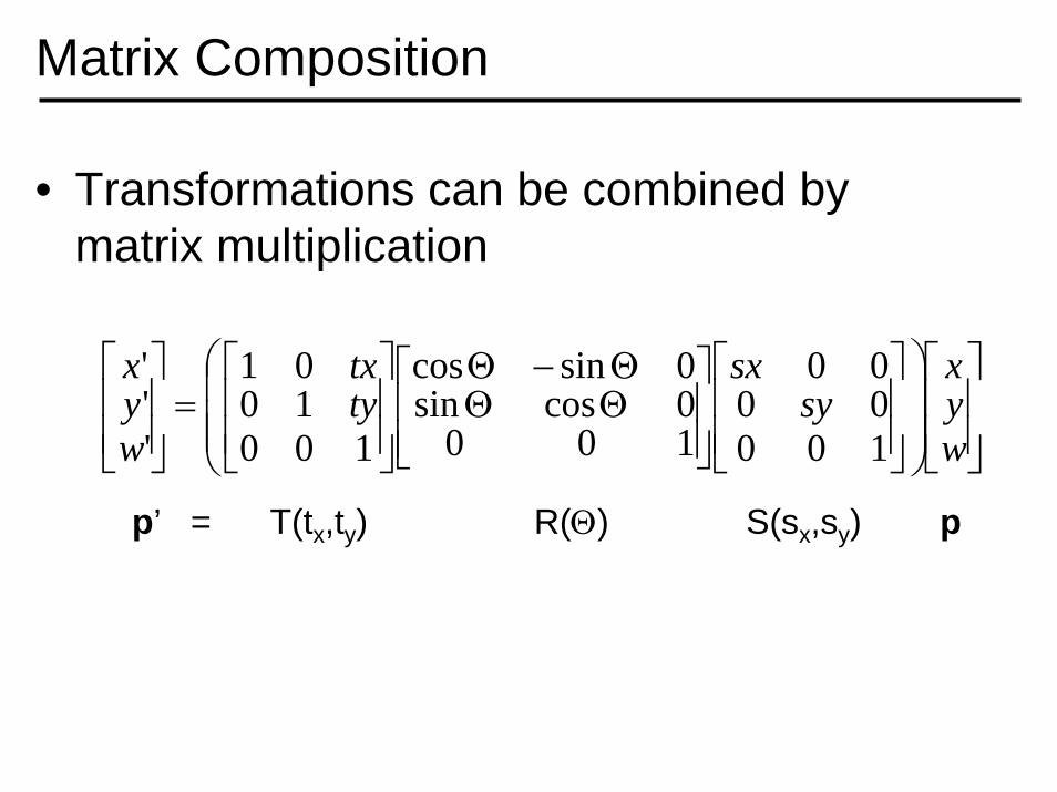
Matrix Composition

• Transformations can be combined by matrix multiplication

⎥⎥⎦

⎤

⎢⎢⎣

⎡

⎟⎟⎟

⎠

⎞

⎜⎜⎜

⎝

⎛

⎥⎥⎦

⎤

⎢⎢⎣

⎡

⎥⎥⎦

⎤

⎢⎢⎣

⎡ΘΘΘ−Θ

⎥⎥⎦

⎤

⎢⎢⎣

⎡=

⎥⎥⎦

⎤

⎢⎢⎣

⎡

wyx

sysx

tytx

wyx

1000000

1000cossin0sincos

1001001

'''

p’ = T(tx,ty) R(Θ) S(sx,sy) p

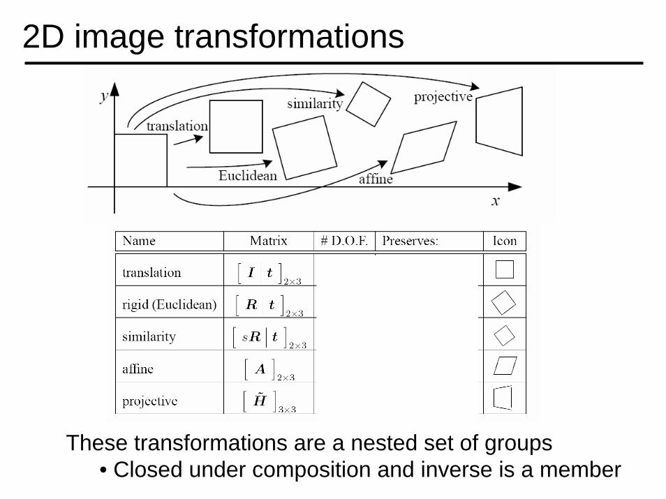
2D image transformations

These transformations are a nested set of groups• Closed under composition and inverse is a member

Recovering Transformations

• What if we know f and g and want to recover the transform T?

x x’

T(x,y)’y y

f(x,y) g(x’,y’)

?

– Using correspondences• How many do we need?

Translation: # correspondences?

• How many correspondences needed for translation?• How many Degrees of Freedom?• What is the transformation matrix?

x x’

T(x,y)’y y

?

⎥⎥⎥

⎦

⎤

⎢⎢⎢

⎣

⎡−−

=100

'10'01

yy

xx

pppp

M

Euclidian: # correspondences?

• How many correspondences needed for translation+rotation?

• How many DOF?

x x’

T(x,y)’y y

?

Affine: # correspondences?

• How many correspondences needed for affine?

• How many DOF?

x x’

T(x,y)’y y

?

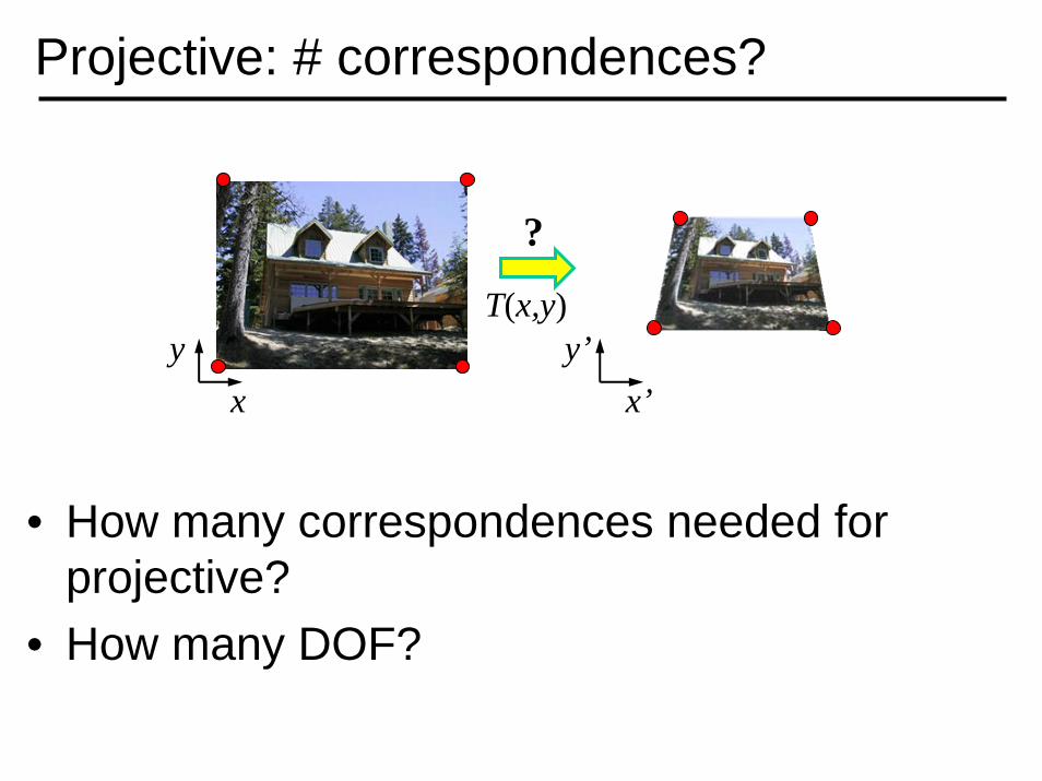
Projective: # correspondences?

• How many correspondences needed for projective?

• How many DOF?

x x’

T(x,y)’y y

?

Example: warping triangles

• Given two triangles: ABC and A’B’C’ in 2D (12 numbers) • Need to find transform T to transfer all pixels from one to

the other.• What kind of transformation is T?• How can we compute the transformation matrix:

T(x,y)

?

A

B

SourceC A’

C’

B’

Destination

⎥⎥⎥

⎦

⎤

⎢⎢⎢

⎣

⎡

⎥⎥⎥

⎦

⎤

⎢⎢⎢

⎣

⎡=

⎥⎥⎥

⎦

⎤

⎢⎢⎢

⎣

⎡

11001''

yx

fedcba

yx

warping triangles (Barycentric Coordinaes)

•Very useful in Graphics…

A

B

A’C’

B’

Source DestinationC

(0,0) (1,0)

(0,1)

changeof basis

Inverse changeof basis

Don’t forget to move the origin too!

2T11−T

Image warping

• Given a coordinate transform (x’,y’) = T(x,y) and a source image f(x,y), how do we compute a transformed image g(x’,y’) = f(T(x,y))?

x x’

T(x,y)

g(x’,y’)

’

f(x,y)

y y

f(x,y) g(x’,y’)

Forward warping

• Send each pixel f(x,y) to its corresponding location

• (x’,y’) = T(x,y) in the second image

x x’

T(x,y)

Q: what if pixel lands “between” two pixels?

y y’

f(x,y) g(x’,y’)

Forward warping

• Send each pixel f(x,y) to its corresponding location • (x’,y’) = T(x,y) in the second image

x x’

T(x,y)

Q: what if pixel lands “between” two pixels?

y y’

A: distribute color among neighboring pixels (x’,y’)– Known as “splatting”

f(x,y) g(x’,y’)xy

Inverse warping

• Get each pixel g(x’,y’) from its corresponding location • (x,y) = T-1(x’,y’) in the first image

x x’y’

T-1(x,y)

Q: what if pixel comes from “between” two pixels?

f(x,y) g(x’,y’)xy

Inverse warping

• Get each pixel g(x’,y’) from its corresponding location • (x,y) = T-1(x’,y’) in the first image

x x’

T-1(x,y)

Q: what if pixel comes from “between” two pixels?

y’

A: Interpolate color value from neighbors– nearest neighbor, bilinear, Gaussian, bicubic

how is project #1 going? - pdfs.semanticscholar.org filewhy is this hard? simple analogy: 11 is the...

Documents