how much scope for a mobility paradox? the relationship between

Citation: Breen, Richard, CarinaMood and Jan O. Jonsson. 2016.“How Much Scope for a MobilityParadox? The Relationship be-tween Social and Income Mobil-ity in Sweden.” Sociological Sci-ence 3: 39-60.Received: March 20, 2015Accepted: April 16, 2015Published: February 4, 2016Editor(s): Jesper Sørensen, KimWeedenDOI: 10.15195/v3.a3Copyright: c© 2016 The Au-thor(s). This open-access articlehas been published under a Cre-ative Commons Attribution Li-cense, which allows unrestricteduse, distribution and reproduc-tion, in any form, as long as theoriginal author and source havebeen credited.cb

How Much Scope for a Mobility Paradox?The Relationship between Social andIncome Mobility in SwedenRichard Breen,a Carina Mood,b, c Jan O. Jonssona, b

a) Oxford University; b) Stockholm University; c) Institute for Futures Studies

Abstract: It is often pointed out that conclusions about intergenerational (parent–child) mobilitycan differ depending on whether we base them on studies of class or income. We analyze empiricallythe degree of overlap in income and social mobility; we demonstrate mathematically the nature oftheir relationship; and we show, using simulations, how intergenerational income correlations relateto relative social mobility rates. Analyzing Swedish longitudinal register data on the incomes andoccupations of over 300,000 parent–child pairs, we find that social mobility accounts for up to 49percent of the observed intergenerational income correlations. This figure is somewhat greater for afine-graded micro-class classification than a five-class schema and somewhat greater for womenthan men. There is a positive relationship between intergenerational social fluidity and incomecorrelations, but it is relatively weak. Our empirical results, and our simulations verify that theoverlap between income mobility and social mobility leaves ample room for the two indicators tomove in different directions over time or show diverse patterns across countries. We explain thecircumstances in which income and social mobility will change together or co-vary positively andthe circumstances in which they will diverge.

Keywords: social mobility; class mobility; income inequality; stratification; intergenerational pro-cesses; intergenerational mobility

INTERGENERATIONAL mobility is a topic studied by both sociologists andeconomists, with the latter focusing on income or earnings mobility (see re-

views by Björklund and Jäntti 2009; Black and Devereux 2011) and the formeron occupational or class mobility (reviewed by Breen and Jonsson 2005). Whensocieties are ranked according to the extent of their economic and social intergener-ational mobility we see a good deal of agreement, with the Scandinavian countriesdisplaying high rates of income mobility and high relative social mobility—or socialfluidity1—and countries such as Britain, Italy and Germany somewhat lower levelsof both (see Breen 2004 for data on social mobility; Corak 2004 and Björklund andJäntti 2009 for income mobility; and Blanden 2013 for international comparisons ofboth). However, there seems to be no consistent relationship between the two formsof mobility. For example, U. S. social fluidity is usually found to be relatively highand similar to that of Sweden and the Netherlands (Beller and Hout 2006, Ferrie2005; cf. Erikson and Goldthorpe 1985) yet the United States has one of the high-est intergenerational income elasticities (and thus the lowest mobility) among theOECD countries (Solon 1992; Zimmerman 1992; Mazumder 2005; Gregg et al. 2013).China may be a similar contradictory case, having a very high intergenerational

39

Breen, Mood and Jonsson How Much Scope for a Mobility Paradox?

elasticity of income (Gong, Leigh and Meng 2010) yet high social fluidity (Ishidaand Miwa 2012).

One strand of the literature holds that income and social mobility simply capturedifferent phenomena. Björklund and Jäntti (2000:22), for example, write that, “froma purely conceptual point of view, . . . class and income . . . are obviously differentaspects of a person’s position in society. Hence, we ought to treat these . . . branchesof mobility analysis as complementary.” Erikson and Goldthorpe (2010:212) takethe same position: “intergenerational income mobility and intergenerational classmobility are of course different phenomena, and there is no a priori reason whythey should change in tandem.” However, it is not difficult to find a different viewof the relationship between income and social mobility, according to which theyare both indicators of a fundamental underlying inequality dynamic—such as theintergenerational reproduction of advantage and disadvantage—which is oftentaken to reflect inequality of opportunity or societal openness (e.g. , Erikson andGoldthorpe 1992). In this view, the ideal objects of analysis—class position, in thecase of sociologists, and lifetime income for economists—claim to capture variationsin life chances; that is ‘the chances an individual has of sharing in the socially createdeconomic or cultural “goods” which typically exist in any given society’ (Giddens1973:130–1). As Blanden, Gregg and Macmillan (2013:542) state, in their comparisonof social and economic mobility trends in the United Kingdom, “The view that weadopt here is that both are trying to assess long-term or permanent socioeconomicstatus but measure it in different ways.” Here discrepancies, such as that foundin the case of the United States, have to be explained in terms of differences in theempirical operationalization of the two forms of mobility.

Whether we accept the idea that the two ways of studying intergenerationalassociations embody something common or take the view that they are different, thefundamental question is the same: how are income and social mobility related, bothformally and empirically? Are they so closely related that divergent trends overtime, or differences in country rankings, should be seen as paradoxes, or are theyso disconnected that viewing them as two indicators of a common phenomenon islikely to be entirely off the mark?

Our first contribution is to address this issue by analyzing the empirical relation-ship between income and social mobility using uniquely suitable population datafrom Sweden that allow us to model the two processes simultaneously and estimatethe intergenerational associations with great precision. In doing so, we follow bothcommon practice and economic theories to design income mobility models. Forsocial mobility, we use the internationally well known Erikson-Goldthorpe (EGP)social class schema (Erikson and Goldthorpe 1992) as well as the more detailedoccupational, or “micro-class”, schema to model social class mobility (Grusky andSorensen 1998). Starting from a framework developed by Björklund and Jäntti(2000), Blanden (2013), and Blanden et al. (2013), we ask how much of the incomecorrelations across generations could be accounted for by social mobility, and weestimate the degree of overlap between income and social class mobility to be30–50 percent. 2 We show this overlap not only for the conventionally reportedfather-to-son association, but take a step further by also studying the impact ofmothers and the outcomes of daughters.

sociological science | www.sociologicalscience.com 40 February 2016 | Volume 3


Our second contribution is to extend this model mathematically in one impor-tant respect, by also considering relative (and not only absolute) social mobilityrates. Through the use of simulations we can show that, given the way in whichsociologists and economists empirically operationalize and analyze mobility, thereis no reason to expect the relationship between the two approaches to be particularlyclose. 3

Intergenerational Mobility

Social Mobility

The study of intergenerational social class mobility has been a mainstay of socio-logical research at least since the 1950s (Carlsson 1958; Featherman and Hauser1978; Erikson and Goldthorpe 1992; Breen 2004). Since the 1980s, mobility tableshave normally been analyzed using loglinear models, for which the basic datumis a table whose cells contain the frequencies in each combination of parent’s andrespondent’s class, usually called origin and destination classes (Hout 1983; Sobel,Hout, and Duncan 1985). A distinction is made between absolute mobility, which isthe pattern of flows from origins to destinations that can be observed in the mobilitytable, and relative mobility or social fluidity captured by odds ratios. These are theratio of the odds, among respondents born into one class origin, compared withthose born into another, of coming to occupy one social class destination ratherthan another. Odds ratios are said to be “margin invariant” because they are un-changed under the multiplication of any row or column of the mobility table by ascalar, permitting comparisons among tables which may have different marginaldistributions.

A log-linear model for the mobility table can be written:

log Fij = λ + λi + λj + λij (1)

where Fij denotes the expected (under the model) frequency in the ijth cell of thetable, where i = 1, . . . , I indexes origins and j = 1, . . . , J indexes destinations. Theorigin and destination (or row and column) main effects are given by λi and λj, andthe origin–destination association parameters are denoted λij. Odds ratios in thetable are functions of λij and not of the other parameters in (1).

There is general agreement on the ranking of countries in terms of their socialfluidity. Sweden, the Netherlands, and Israel belong to the group of more sociallyfluid countries, while Germany, Italy, and Ireland are characterized by a low levelof fluidity (Breen and Luijkx 2004). Though comparisons are not straightforward(mainly because of the difficulties of deriving, from US occupational codes, aclass classification comparable to the Erikson-Goldthorpe schema used in mostcomparative research), it seems that the United States is characterized by high socialfluidity (Breen and Jonsson 2005), not far off the Swedish figure (Jonsson et al. 2009).



Income Mobility

The study of intergenerational income mobility is a rapidly growing research areawithin economics (for important contributions, see Atkinson 1983; Solon 1992;Zimmerman 1992; Corak 2004). It focuses on the parent–child (usually father–son)correlation or elasticity of income or earnings. Normally, researchers relate thechild’s income as an adult to his or her parent’s income using a regression model:

log(yic) = α + β log(yip) + εi. (2)

Here i denotes a family (a parent–child pair), yip is parental income and yic is child’sincome. The average log income among children is captured in α, while β, theregression coefficient, estimates the intergenerational elasticity of incomes. Theerror term, ε, is assumed independent of parental income. β can be interpretedas the fraction of the income differences among parents that are transmitted tochildren. An intergenerational elasticity of around 03 means that almost a thirdof the income differences of two randomly chosen parents in a population will onaverage, be found among their children. This representation of intergenerationalmobility is a summary measure and as such suffers from the typical weaknesses ofsummary measures, but it can be made more complex by including non-linearities(e.g., Bratsberg et al. 2007). However, precisely because the elasticity is a summaryindicator it is very useful for assessing differences between countries. In generalterms it seems income mobility is higher in the Nordic countries and in Canadathan in the Unites States, the United Kingdom, Germany, France, and Italy—thoughseveral of the estimates reported in the international literature are surrounded bylarge standard errors.

A minimum requirement for this kind of analysis is data on a parent and his orher child’s income, and such data are difficult to obtain, and, even when available,usually relate to different age-ranges of the parents and children. Because incomestypically increase with age, in particular for those in higher social positions, it isusual to add age and the square of age to the specification of equation (2). Further-more, economists ideally seek to measure “permanent or “lifetime” income and forthis many years’ income data are necessary in order to average out transitory in-come components. Early estimates of income mobility in the United States reportedan elasticity lower than 0.20, but later studies, using more years of parental income,yielded estimates around 0.40 (Solon 1992; Zimmerman 1992). Mazumder (2005)using very long-run measures of parental earnings, claimed that US elasticity couldbe as high as 0.6, a result also arrived at by Gregg et al. (2013) when correcting theU.S. elasticity for measurement error.

Sociologists who study social mobility are most often interested in the un-derlying association between parents’ and children’s class in the mobility table,controlling for the different marginal distributions of origins and destinations (i.e.,structural differences between parents’ and children’s class distributions). But it isuncommon to find a similar approach among economists. The elasticity dependson both the correlation between parents’ and children’s (log) incomes and the ra-tio of the standard deviations of each. If we believe that the former captures theunderlying parent–child income association, we can transform the elasticity into



a correlation by multiplying it by the ratio of the standard deviation of the log ofparent’s income, σp to the standard deviation of child’s log income, σc:

r = βσp

σc, (3)

so giving a measure more in line with the sociologists’ use of odds ratios. Becauseit is not yet common practice to report intergenerational income correlations, weare uncertain about differences between countries or trends over time in the inter-generational correlation. For Sweden, however, Jonsson, Mood and Bihagen (2010)showed that the intergenerational household income correlation decreased for 33–37-year-olds during the period 1993–2007, while the elasticities increased, thusdemonstrating the advisability of considering both types of income associations.

The Mathematical Relationship between Income Mobilityand Social Mobility

A reviewer of the literatures in social and income mobility could not fail to be struckby the very limited degree to which they engage each other. Some commentatorshave certainly drawn attention to parallel findings in the two literatures (Swedenand Scandinavia most fluid) and to some striking discrepancies of which the UnitedStates provides a good example. Björklund and Jäntti (2000) sought to reconcileeconomic and social mobility by expressing the relationship between them in a sim-ple model of how much of the intergenerational income correlation is mediated viaintergenerational social mobility (or persistence). Here we follow their exposition.

Write income in each generation as a function of social class and a residual term:

yip = yp + ∑j

bjpxijp + eip (4)

for one or both parents (most often the father), and

yic = yc + ∑j

bjcxijc + eic (5)

for the child. Here y is income,4 j indexes social classes (j = 1, . . . J), xij are dummyvariables indicating which class is occupied, the b’s capture mean income in eachclass expressed as the deviation from overall mean income, yp and yc, and e is aresidual term, uncorrelated with class,5 which captures within-class variation in logincome. It will be useful to write the coefficients in matrix form, so bp and bc areboth J × 1 vectors of mean income in each class measured as the deviations fromthe overall mean in the parent and child classes.

Björklund and Jäntti (2000) argued that the covariance between yipand yic couldbe expressed as the sum of two paths. The first path, proceeding via social class,is given by the product of the effects of class on income in each generation andthe joint distribution of parent’s and child’s class: i.e., b′pP(XpXc)bc. This capturesthat part of the intergenerational covariance in income due to intergenerational



e(P) b(P)

cov(e(P),X(C)) cov(e(C),X(P)) cov(e(P),e(C)) M

e(C) b(C)

Parental income

Child's income

Other factors Parent

Other factors Child

Parental class

Child's class

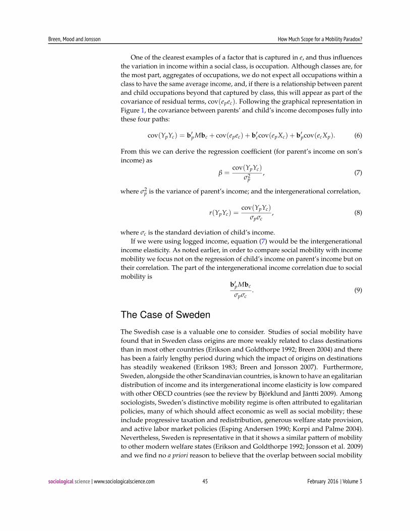
Figure 1: The Income and Social Mobility Process

class mobility. The second path is equal to cov(epec) and captures the impact of thetransmission of factors other than class. Björklund and Jäntti’s insight, however,was to see that P(XpXc) is the mobility table; that is, the cross-tabulation of parent’sby child’s class, albeit normed by dividing the frequencies of the table by the samplesize. So we now write M ≡ P(XpXc) for notational convenience.

Blanden et al. (2013) pointed out, however, that these two paths are not exhaus-tive of the ways in which parental and child incomes may be linked. There may becovariances between, on the one hand, the residual term in the parent’s equationand child’s class position, which establishes a path between parent’s and child’sincome equal to cov(epXc)bc, and between the residual from the child’s equationand parental class, giving rise to the path cov(ecXb)bp.

Figure 1 presents the resulting model of the relationship between income andclass mobility, with parental characteristics in the upper part and filial in the lower.The thick vertical arrow represents the intergenerational covariance of incomes: ourgoal is to explain how intergenerational class mobility contributes to generatingthis covariance. On the right side of the figure we see the arrow linking parent’sand child’s class and on the left side the covariance between the error terms ofequations (4) and (5). The elements added by Blanden et al (2013) are shown bythe diagonal lines linking parent and child, and they allow for the possibility thatfactors independent of parent’s class but related to parent’s income are correlatedwith child’s class position, and that parent’s class is correlated with other childfactors, independent of child’s class, that influence child’s income. We could thinkof a number of characteristics that we do not observe in normal mobility studiesthat exemplify these diagonal links. The variation within classes in educationalqualifications, skills, and abilities are obvious examples and, when such characteris-tics are measured (mostly at the child level, where data are more readily available),they account for some—but not all—of the intergenerational income correlation(Blanden, Gregg, and Macmillan 2007; Mood et al. 2012). In many traditionalstudies using only information on fathers, the error term on the parental side willof course include those characteristics of mothers that are unrelated to father’s classbut related to his income.



One of the clearest examples of a factor that is captured in e, and thus influencesthe variation in income within a social class, is occupation. Although classes are, forthe most part, aggregates of occupations, we do not expect all occupations within aclass to have the same average income, and, if there is a relationship between parentand child occupations beyond that captured by class, this will appear as part of thecovariance of residual terms, cov(epec). Following the graphical representation inFigure 1, the covariance between parents’ and child’s income decomposes fully intothese four paths:

cov(YpYc) = b′p Mbc + cov(epec) + b′ccov(epXc) + b′pcov(ecXp). (6)

From this we can derive the regression coefficient (for parent’s income on son’sincome) as

β =cov(YpYc)

σ2p

, (7)

where σ2p is the variance of parent’s income; and the intergenerational correlation,

r(YpYc) =cov(YpYc)

σpσc, (8)

where σc is the standard deviation of child’s income.If we were using logged income, equation (7) would be the intergenerational

income elasticity. As noted earlier, in order to compare social mobility with incomemobility we focus not on the regression of child’s income on parent’s income but ontheir correlation. The part of the intergenerational income correlation due to socialmobility is

b′p Mbc

σpσc. (9)

The Case of Sweden

The Swedish case is a valuable one to consider. Studies of social mobility havefound that in Sweden class origins are more weakly related to class destinationsthan in most other countries (Erikson and Goldthorpe 1992; Breen 2004) and therehas been a fairly lengthy period during which the impact of origins on destinationshas steadily weakened (Erikson 1983; Breen and Jonsson 2007). Furthermore,Sweden, alongside the other Scandinavian countries, is known to have an egalitariandistribution of income and its intergenerational income elasticity is low comparedwith other OECD countries (see the review by Björklund and Jäntti 2009). Amongsociologists, Sweden’s distinctive mobility regime is often attributed to egalitarianpolicies, many of which should affect economic as well as social mobility; theseinclude progressive taxation and redistribution, generous welfare state provision,and active labor market policies (Esping Andersen 1990; Korpi and Palme 2004).Nevertheless, Sweden is representative in that it shows a similar pattern of mobilityto other modern welfare states (Erikson and Goldthorpe 1992; Jonsson et al. 2009)and we find no a priori reason to believe that the overlap between social mobility



and income mobility should be much different from what we expect from otherEuropean countries.

Although there are good substantive grounds for choosing Sweden as a testcase, there is also a practical reason: there are very few, if any, data sets in the worldoutside of the Scandinavian countries that can provide similarly high quality dataand a sufficiently large sample for the kind of simultaneous analysis of social andeconomic intergenerational mobility that we undertake.

Data and Variables

We estimate economic and social mobility, and the individual components of equa-tion (6), using data from official Swedish registers, primarily tax registers andcensuses, kept by Statistics Sweden for the Swedish Institute for Social Research.To address different aspects of the intergenerational associations, we use not onlyincome and social class for fathers (as is common in the literature) but also fam-ily income and the dominant class in the parental generation (the dominant classhere defined as the higher of father’s and mother’s class). Daughters and sons areanalyzed separately, and their outcomes are studied in terms of social class andboth personal and family income. We selected children born 1948–52 and, througha unique personal multi-generational identifier we added information on theirparents, giving us data on around 300,000 father–child pairs (the exact number ofobservations varies between the analyses depending on the combination of incomeand class variables).6

We use two income measures: personal (own) employment income, defined asthe sum of pre-tax income from business, employment and work-related benefits;and disposable family income, defined as the sum of the family’s employment andbenefit incomes after the deduction of taxes. We take the average of parents’ yearlyincomes in 1968–19727 and the average of the child’s incomes in 1988–92 (whentheir ages ranged from 36–40 in 1988 to 40–45 in 1992). These years are chosenbecause their midpoints are the censuses of 1970 and 1990, respectively, from whichwe draw occupational information. For parental disposable family income we takethe average of mother’s and father’s incomes (including cases where the motherand father do not live together). We use income spells only if at least three out offive of these years were non-missing. Income is top-coded for incomes four or morestandard deviations above the mean (this affects one percent of sons in each cohortand three percent of their fathers), and years with zero or negative incomes havebeen coded missing. We also exclude those who are reported as self-employed inany of the censuses, as their registered incomes are less reliable indicators of actualliving standards.

Occupation is measured by information from the censuses in 1970 (for parents)and 1990 (for children), coded according to the Swedish standard classification,NYK (Statistics Sweden 1989). These data are used to construct classes in twodifferent degrees of aggregation. The first is a “big-class” scheme, closely related tothe EGP class schema. Because we omit the self-employed and farmers from ouranalyses, the usual seven EGP classes are reduced to five, and these are describedin the note at the foot of Table 1 (the Roman numerals refer to the EGP classes.)8



The second class schema is built on occupations, or “micro-classes,” definedas occupational categories that share common features in the technical-functionaldivision of labour, including skill requirements, training, and working conditions(Grusky 2005). We define 77 micro-classes, based on the coding algorithm pre-sented in Jonsson et al. (2009; see Table A2 in the appendix), and described atwww.classmobility.org9 We expect the occupational groupings to pick up incomevariation within big classes, thus shedding light on what the maximum overlap be-tween social and economic mobility might be. Knowing the difference between thetwo class schemata in this respect is useful given that, in most normal (survey) datasets, it is not possible to use more than five to ten classes. For both class schemata,we use the individual’s own class and also the family’s dominant class, wheredominant class is the class of the parent whose occupation has the higher status,using the Standard International Occupational Prestige Score (SIOPS) occupationalscale for ranking (Ganzeboom and Treiman 1996).

Descriptives

Table 1 shows descriptive statistics. Panel A displays the distribution of class originsand destinations for father, mother, son, and daughter, and for the dominant originand destination class distributions. Comparing fathers and sons, we see the wellknown upgrading of the class structure (here, between 1970 and 1990), with theupper middle class (I) expansion from nine to 21 percent and the correspondingdecline of the working classes (VI and VII) from 59 to 44 percent. Comparingsons and daughters also brings out much of the gender inequality in modern labormarkets, with women being concentrated in lower-grade manual (VII) and non-manual (III) jobs, and being much less represented in professional and managerialpositions (I). But we also note the rapid upgrading of women’s class positions whencomparing daughters with their mothers. Mothers’ labor market attachment in 1970was still weak (43 percent had no recorded occupation) and dominated by unskilledmanual work; this large discrepancy between mothers and daughters explains whywe do not conduct mobility analysis between them. The distribution of dominant(“household”) class origin is similar to that of father’s class, but because we includethe whole population here (some of whom grew up without a father), there aresome small dissimilarities. The minor differences between sons’ and daughters’household class distributions are due to the class destinations of single people.

Panel B shows, as an example of the social fluidity for our cohorts, the adjacentodds ratios from the father–son mobility table that cross-tabulates father’s classin 1970 with son’s class in 1990. The pattern of odds ratios will be familiar tostudents of intergenerational class mobility, with the largest values being on the(shaded) main diagonal, indicating the marked tendency for intergenerational classpersistence.


www.classmobility.org


Table 1: Descriptive statistics for intergenerational mobilityPanel A: Distribution of EGP origin and destination classes for children with valid value on own and father’sclass, and own and father’s employment income

Parents’ class Own classFather 1970 Mother 1970 Son 1990 Daughter 1990

EGP Class N of cases % N of cases % N of cases % N of cases %

I 26,442 9 3,786 1 33,502 21 1,7274 11II 45,467 15 26,155 8 36,520 23 40,122 26III 52,963 17 20,115 7 17,874 11 39,520 26VI 96,996 31 5,492 2 35,407 23 15,720 10VII 86,187 28 120,047 39 32,540 21 39,576 26Missing 132,460 43Total 308,055 100 308,055 100 155,843 99 152,212 99

Dominant classParents’ 1970 Sons’ 1990 Daughters’ 1990

EGP Class N of cases % N of cases % N of cases %I 31,397 8 46,631 23 46,753 23II 70,391 17 56,158 28 58,378 29III 65,207 16 32,262 16 39,498 20VI 99,266 24 36,491 18 27,676 14VII 139,519 34 32,518 16 29,415 15Total 405,780 99 204,060 101 201,720 101

Note: EGP classes: I=Upper middle class (professionals, higher administrative, executives), II=Middle class (semi-professionals [e.g.,nurses], mid-level administrative, low-level managers), III=Routine non-manual (clerks, secretaries, office-workers), VI=skilled manualworkers, VII=unskilled manual workers. Self-employed (classes IV) are not included in the analysis.

Panel B: Adjacent Odds Ratios in Intergenerational Class Mobility table

Son’s EGP class 1990Father’s EGP class 1970 I vs II II vs III III vs VI VI vs VII

Upper middle (I) vs Middle class (II) 1.69 1.03 1.47 0.77Middle class (II) vs Routine non-manual (III) 1.27 1.23 1.43 0.92Routine non-manual (III) vs Skilled manual (VI) 1.42 0.92 2.15 0.85Skilled manual (VI) vs Unskilled manual (VII) 0.98 1.21 0.86 1.42

Panel C: Parents’ and children’s income in 2007 Swedish kronor (for children with valid value on own andfather’s class, and own and father’s employment income)

Parents’ income 1970 Mean Median Std dev Min Max N of cases

Father, employment 250,955 213,342 140,988 1,775 106,1419 30,8055Mother, employment 95,034 85,642 62,512 85 407,154 221,613Household disposable 205,732 191,038 84,982 34,955 77,7606 308,000

Child’s income 1990

Son employment 274,810 254,450 97,907 3,636 68,7570 15,5843Daughter, employment 180,887 175,615 65,648 1,267 671,995 152,212Son household disp 31,8576 321,110 107,177 10,700 107,9791 155,842Daughter, household disp 327,039 330,294 112,830 12,983 1,079,791 152,209

Notes: Zero-incomes and negative incomes not included. Incomes top-coded to maximum four standard deviations from the meanExchange rates as of 2007 (July 1st): 10 SEK=1423 USD; 1061 Euro; 71 GBP.

Panel D: Age of parents and children (for children with valid value on own and father’s class and own andfather’s employment income)

Mean Median Std dev Min Max N

Father’s age 1970 51 50 6.2 28 75 308,055Mother’s age 1970 48 47 5.9 27 75 300,045Child’s age 199 40 40 1.4 38 42 308,055

Notes: 75 is the maximum age in the data. The very young minimum ages of parents are explained by adoptions.



Panel C of Table 1 shows the average and dispersion of parents’ and children’sincomes, with all amounts expressed in 2007 Swedish kronor (exchange rates inthe note to the table). Real incomes have grown over time and, given the rapidlyincreasing labor market participation of women, this is especially so for householddisposable incomes. Though income from employment reflects gender inequalityfavoring men, women, nevertheless, have slightly higher disposable householdincomes (assuming a gender-neutral distribution within families). This is probablybecause single women tend to have higher levels of education than single men, andbecause women’s spouses are usually older than men’s.

Finally, panel D shows the descriptive statistics for age. Children’s incomesare measured when they are around 40, but parents are about 10 years older, onaverage, when their incomes are measured, and they display much greater variationin age.

Results

There are several ways of conceiving of and defining the intergenerational incomecorrelation. We use three specifications, derived from previous studies and existingtheory. Our first specification focuses on the relationship between father’s andchild’s own income from work and on father’s and child’s individual class. This iscommon practice in both the income and social mobility literature, where mother’sand spouse’s class or income are commonly ignored; we call this the standard model.Our second specification, which we call the origin family model, replaces father’swork income and father’s own class with a measure of disposable family incomeand a measure of class origins based on the dominant class position of father ormother, but it retains the individual work income and class for children. This modelseeks to capture origins more fully by including the income and class position ofboth parents. It comes closest to the Becker and Tomes (1986) child investmentmodel, which posits that it is the total economic resources in the household thatinfluence children’s educational and income opportunities.

Our third and last specification—the gross model—takes the origin family modeland replaces the individual income and class measures of the child with his or herdisposable family income and a dominance measure of class (based on whicheverof the child or child’s spouse’s class is considered dominant). This gross modelmeasures family, rather than individual, resources in both generations. As a con-sequence it captures not only the direct transmission of income from origin todestination family but also the effects of assortative mating in the child generation.

Applying these three specifications to samples of male and female respondentsgenerates six income correlations, shown in Figure 2. The correlations are larger formen than for women. This finding, common in the literature on economic mobility(see Lee and Solon 2009) is, to some extent, a consequence of the gender gap inearnings that introduces a source of father–daughter economic mobility that has nocounterpart in the father–son comparison.

For both sexes the correlations are greatest in the standard model and weakestin the gross model. The latter result is expected, given that the gross model includesthe impact of spouse’s income, which, despite the tendency towards assortative



0.00

0.10

0.20

0.30

Model 1 Model 2 Model 3

Inco

me

corr

elat

ion

Men

Women

Figure 2: Income correlation between parents (average incomes 1968–72) and children (average incomes1988–92, adjusted for inflation) for sons and daughters born 1948–52, for three models of intergenerationalcorrelations(models explained below).Model 1: Father’s employment income, child’s employment incomeModel 2: Parents’ household income, child’s employment incomeModel 3: Parents’ household income, child’s household income.

mating, dilutes the intergenerational correlation. Nonetheless, this is the trueassociation between disposable incomes in the family of origin and the family ofdestination. That the income of the father alone is a better predictor of sons’ incomesthan the income of father and mother together, and the finding that this is not so forwomen, is probably a further manifestation of the gender gap in earnings. Addingmother’s income to father’s income adds noise to the father–son, but not to thefather–daughter, correlation.

Next, we decompose the income correlations from Figure 2 into the four partsshown in equation (6), using both of our two measures of social class—the EGPfive-class schema and the 77 micro-classes. The coefficients are generated frommodels that include age and age squared, but this makes almost no difference to theresults (coefficients with and without age controls differ only at the third decimalplace). Figure 3 shows how much of the intergenerational income correlation isaccounted for by intergenerational social persistence (in Table A1 of in the appendixwe present the full results for each of the 12 decompositions).

As Figure 3 shows, in the standard model among men, intergenerational persis-tence between EGP classes accounts for 39 percent of the intergenerational correla-tion of father–son incomes. The remaining three terms—the correlation betweenthe errors, the correlation between the parental error and child’s class and thecorrelation between parental class and child’s error—each accounts for around 20percent (Table A1). Moving to the origin family model, the share of the correlation



0.00

0.10

0.20

0.30

0.40

0.50

0.60

Model 1 Model 2 Model 3

Pro

po

rtio

n o

verl

ap

Men EGP class

Men Micro-class

Women EGP class

Women Micro-class

Figure 3: The degree of overlap between income correlation and social mobility for three models of intergener-ational correlations (models explained below).Model 1: Father’s employment income and class, child’s employment income and classModel 2: Parents’ household income and class, child’s employment income and classModel 3: Parents’ household income and class, child’s household income and class

in incomes (which we saw in Figure 2) accounted for by class persistence declinesto 37 percent for men; in the gross model it declines to 33. This is predominantlybecause the correlation of the errors increases from 23 percent in the standard modelto 32 percent in the gross model (Tabel A1). This means that factors that vary withinsocial classes—even within micro-classes—and that do not influence children’ssocial class position account for a bigger portion of the intergenerational incomecorrelation in the family origin model and the gross model. In the standard model(fathers only), this is likely to be due in part to characteristics of the mother (suchas her education). In the gross model, which includes spouse’s income, this pathmay be capturing the consequences of assortative mating (such as attributes of theparents-in-law).

The use of the 77 micro-class mobility table increases the degree to which classmobility and income mobility are directly related: in the standard model applied tomen, micro-class persistence accounts for almost 46 percent of the intergenerationalcorrelation (compared with 39 percent for EGP class mobility). As expected, theuse of a finer class classification reduces within-class variation and so the impact ofthe correlation between the errors is lessened. This is also true of the other modelspecifications for men: micro-class persistence accounts for more of the incomecorrelation even though the impact of class mobility diminishes as we move fromthe standard model to the origin family model and then the gross model. Overall,however, the improvement brought about by moving from five to 77 classes is



quite modest. The reason for this is most likely that micro-classes largely capturea lateral dimension in the class structure that is rather weakly related to incomein Sweden. Although the differences in social networks, skills, and occupationalaspirations between, say, bakers, metal workers, and carpenters may be essential forsocial class inheritance, they do not necessarily imply any income differences. This,in turn, reflects the different processes supposed to generate social and economicpersistence, respectively, but here it is best to caution against generalizing beyondthe case of Sweden.

The results for women (daughters) are both similar to and different from thoseof men. For our main question, the most striking difference is that class persis-tence accounts for more of the income correlation—almost half in the standardmodel, falling to 38 percent in the gross model (Figure 3), and the residual corre-lation accounts for less of the overlap among women than among men (Table A1).This difference may come about because men’s disproportionate frequency amonghigh-income earners leads to larger within-class variation in income, and the char-acteristics that account for this can be expected to be correlated across generations.The micro-class model picks up parts of this residual for men, suggesting that someof the unobserved characteristics are related to occupations (such as occupation-specific skills, qualifications, or aspirations). For women, on the other hand, themicro-classes perform particularly poorly: indeed, in the origin family model andthe gross model, micro-class persistence accounts for less of the intergenerationalincome correlation than does EGP class persistence. This is most likely becausethe relationship between parental class (which is predominantly the father’s ratherthan mother’s class in the dominance approach) and daughter’s class is stronger atthe EGP big-class level than at the level of micro-classes due to occupational gendersegregation (Jonsson et al. 2009).

When we move from the conventional model (involving fathers only) to thefamily origin model, and also to the gross model, we bring in mothers’ incomeand class. If it were the case that there were a gender interaction in the mobilityprocess, the decline in the share of the income correlation accounted for by socialpersistence across models would not have been as sharp for women. Instead, wefind a similar decline for women as for men when we move from the standard to thegross model, and the residual part of the intergenerational correlation increases evenmore for daughters. This result suggests that there is no obvious mother–daughterinteraction in the mobility process.

Social Fluidity and Intergenerational Income Mobility

Thus far our decomposition has followed that of Björklund and Jäntti (2000), asdeveloped by Blanden et al (2013). However, Björklund and Jäntti’s attempt toreconcile economic and social mobility did not fully reflect how sociologists analyzesocial mobility because their decomposition relates economic mobility to absolutesocial mobility, rather than to relative mobility. The finding of high mobility in theUnited States, for example, is actually a finding of high social fluidity, and thisis something to which the decomposition shown in equation (6) does not speak



directly. As noted earlier, one of the goals of this paper is to make good thatomission.

This presents a difficulty because the frequencies of a mobility table cannotbe written as a linear or a log-linear function of odds ratios alone and so there isno analytical expression for the relationship between social fluidity and economicmobility. Instead we proceed by simulation. Using the method described in theappendix, we generate a set of hypothetical mobility tables, each of which has thesame marginal distributions as the observed Swedish mobility table but with logodds ratios uniformly weaker or stronger than those observed. We change thestrength of the log odds ratios by multiplying the log-linear model’s interactionparameters by a scalar, s, which we vary from 0.1 to 4. Each value of s gives rise to acounterfactual mobility table, Ms. By using these counterfactual tables to calculatethat part of the income correlation due to social mobility, we can see how varyingsocial fluidity (weaker or stronger odds ratios) leads to different intergenerationalincome correlations.

Figure 4 plots the relationship between the income correlation implied by socialmobility for different degrees of social fluidity in the Swedish data, using tablesgenerated by the method described in the appendix. The x-axis shows the scaling—this is the value by which the log odds ratios in the original table have beenmultiplied to generate the counterfactual tables used in the computation of thecorrelation. Thus the value of the correlation when the scaling equals one is theobserved implied mobility correlation, 0.126. As Figure 4 shows, as the associationbetween origins and destinations in the mobility table increases, so does the impliedintergenerational income correlation, reflecting the fact that the covariance of originsand destinations itself increases as the odds ratios in the table become larger. As theodds ratios become very large—that is, more than twice as large as in the Swedishdata—the relationship grows at a weakening rate, so that, at very low levels ofsocial fluidity (high levels of association), further reductions in fluidity have lesseffect on the intergenerational income correlation.

The concave shape of the line in Figure 4 arises because, for a given set ofmarginal distributions of origins and destinations and for the patterns of oddsratios shown in panel B of Table 1, as the odds ratios capturing the associationbetween origins and destinations grow larger, an increasing share of cases clusterson the main diagonal, maximizing the covariance of origins and destinations10

But this clustering is subject to the constraint that the marginal distributions arefixed, and thus the share of cases on the main diagonal has a limit and so, therefore,does the overall covariance of origins and destinations. In turn this means that thecorrelation of parent–child incomes arising through intergenerational persistencealso tends towards a limit (given fixed values of bp and bc). Expressing this moreformally, let Qs denote the share of cases on the main diagonal of table Ms and ρs

be the income correlation due to intergenerational persistence when Ms is usedin equation (6), the decomposition. Then we find that, as s → ∞, Qs → Q∗ andas Qs → Q∗, ρs → ρ∗. That is, as s becomes large, the share of cases on themain diagonal reaches a limiting, maximum value (Q∗); in our Swedish data themaximum share of cases on the main diagonal is 0.584. As the share of casesreaches its limit, so does the implied income correlation (its limit is ρ∗): in the



0"

0,05"

0,1"

0,15"

0,2"

0,25"

0,3"

0,1" 0,6" 1,1" 1,6" 2,1" 2,6" 3,1" 3,6"

Implied"income"correla5

on"

Scaling"of"odds"ra5os"in"social"mobility"table"!

Figure 4: The relationship between the income correlation implied by social mobility for different degrees ofsocial fluidity

case of Swedish men this is 0.306. But this limit is approached very slowly. Themaximum implied correlation shown in Figure 4 is 0.259, and this corresponds toan origin–destination association four times greater than that observed in Sweden.The limit of 0.306 in fact exists at a point far beyond the (lower) range of socialfluidity observed in previous studies11 Over the observed range the relationshipbetween fluidity and economic mobility is approximately linear.

Notice that changing fluidity will not, of itself, change the variance of eitherparent or child incomes. To see this we can draw on equations (4) and (5) (butbearing in mind that we are now using un-logged incomes) to write

σ2p = b′pVX(p)bp + var (ep), (10)

where VX(p) is the variance-covariance matrix of the parental class dummies andvar (ep) is the within-class variation in parental incomes. We can write the equiva-

lent expression for the variance of child incomes:

σ2c = b′cVX(c)bc + var (ec). (11)

The important point is that VX(p) and VX(c) both depend only on the marginaldistributions of origins and destinations and these are unaffected by changing theassociation in the mobility table. Thus, although variations in hypothetical fluidityin a given table affect the origin–destination covariance, they do not affect thevariance of either origins or destinations.



How are Economic and Social Mobility Related?

The relationship between social and economic mobility depends on: (1) the strengthof the relationship between class and income among parents and among children;and (2) the covariance between parents’ and children’s class position. In turn, thiscovariance depends on (2a) social fluidity; and (2b) the marginal distributions oforigins and destinations. Because these elements can vary independently we shouldnot expect to see any necessary empirical relationship between social fluidity andthe intergenerational income correlation. Nevertheless, if we hold two of themconstant, we can state how variation in the third will be related to variation in theintergenerational income correlation.

Consider first the case in which the relationships between origins and parentalincome and between destination and child’s income are held constant, and so are themarginal distributions of origins and destinations. Then, declining odds ratios inthe mobility table (increasing social fluidity) will, as our simulations in the previoussection showed, reduce the covariance between origins and destinations, and thiswill drive down the intergenerational income correlation. Thus, more social fluiditywill, as we might have hoped, be associated with more income mobility. Nowconsider the situation in which the class–income relationships are held constantand so are the odds ratios in the mobility table: in this case, the more similarare the distributions of origins and destinations the greater the intergenerationalcorrelation of incomes. If Swedish sons had the same marginal class distribution astheir fathers, the intergenerational income correlation implied by social persistencewould increase from its observed 0.126 to 0.186.

Finally, consider the case when the covariance of origins and destinations isfixed. The more strongly class is related to income the stronger the relationshipbetween class and income mobility. When class is more predictive of income, theratio of the between-class to within-class variance in income among both parentsand children will be large; average income differences between classes, captured inthe vectors bp and bc will also be large; and the three terms in equation (??) thatinvolve the residuals—namely the residual covariance, cov(epec), the correlationbetween parental residual and child’s class, cov(epXc), and the correlation betweenparental class and child’s residual, cov(ecXp)—will be small and so income mobilitywill be more closely linked to social mobility.

Conclusions

Recent research on the transmission of advantage and disadvantage across gen-erations has seen a burgeoning literature on income mobility as an alternative, ora complement, to the study of social class mobility. These studies have howeverreported seemingly paradoxical results—the United States, for example, has beenportrayed as a relatively equal country in terms of social mobility, but as highlyunequal in terms of income mobility. How, then, are social and income mobilityrelated? Our contribution to answering this challenging question is to measure theirrelationship empirically, using data from Swedish population registers and censuses



that are specially suitable for this endeavor; and to understand the relationshipmathematically.

We find, for the standard father-to-son model, that the intergenerational incomecorrelation implied by the pattern of intergenerational class persistence is 0.12 whenusing a five-class schema and 0.14 when we used a 77 micro-class, or occupational,classification. These represent 39 and 46 percent, respectively, of the observedincome correlation of 0.3. We extended this model in several ways: by includingdaughters; by bringing in mothers’ incomes to form a total household income thatis integral to the child investment model; and by using total household incomeboth for parents and children, so that the intergenerational income correlationincludes the effect of origin on partner selection. The intergenerational correlationsfor daughters are lower than for sons, irrespective of the definition of parentalincome, but the part accounted for by social persistence is generally higher. Forsons, the residual income correlation (not involving class in either generation)is high, suggesting that characteristics of fathers that vary within classes have astrong effect on sons’ incomes. Though these characteristics may include thosewe normally do not observe (such as skills, abilities, aspirations, and networks),we find that replacing the EGP five-class schema with 77 micro-classes accountsfor some of this residual, suggesting that these characteristics are, in part, relatedto occupations. However, for women, the five-class schema accounts for more ofthe intergenerational income correlation than the 77 micro-class schema. This, webelieve, is predominantly an effect of occupational gender segregation, which leadsto a mismatch of fathers’ and daughters’ occupations, meaning that the micro-classmobility table is more erratic for the father–daughter combination, and so accountsfor less of the income correlation than the five-class mobility table.

There are good grounds for supposing that the percentage accruing to thefive-class schema is high because of Sweden’s centralized wage bargaining anda relatively regulated labor market, with the concomitant low variations in wagewithin social classes. This is unlikely to be the case in the liberal regime countrieslike the United Kingdom and the United States, where the difference in resultsbetween a more and less aggregated class schema might be expected to be greater.Indeed, it may be that countries such as the United States and China appear to beoutliers in the social/income mobility relationship because most of the data wehave on both types of intergenerational mobility comes from European societies, inmany of which labor market regulations and centralized wage bargaining may leadto a closer relationship between class and income than exists in other parts of theworld.

This brings us back, finally, to the question of whether social and income mobilityshould be seen as two ways of measuring some underlying concept of inequality,or whether they capture distinct social processes. We have not addressed theconceptual issue here but rather attempted to contribute by analyzing the overlapempirically and mathematically. Our overall conclusion is that social fluidity andincome mobility are positively related, but whether we observe such a relationshipbetween them is contingent on variation in other circumstances, specifically thedegree to which class and income are associated among parents and children, andthe degree of similarity in the distributions of origins and destinations. If we wanted



to uncover the empirical relationship between social fluidity and income mobility(for example, if we had measures of the two for a number of countries) we wouldalso need to take account of differences in these other circumstances. Furthermore,the relationship between the two will also depend on how we measure class andincome, and whether we study men or women—the overlap between social andincome mobility ranges from 32 to 49 percent in our analyses of Swedish data, andthis range may be greater with other mobility models and with data from othercountries.

That some countries rank quite differently on social fluidity and income mobilityhas often been thought paradoxical but, as we have shown, there is no paradox. Theapproach taken in this paper sets out the means by which the relationship betweensocial and income mobility in any specific case may be made more intelligible.

Notes

1 Social fluidity refers to relative mobility rates comparing the class distributions of peoplefrom different social class origins. These relative rates are captured through odds ratios,as we explain below.

2 We could also have asked how much of social mobility can be accounted for by incomemobility. This leads to a more cumbersome analysis, but the mathematical relationshipis shown in Appendix B.

3 We should stress that we are not seeking to make a causal claim about the extent towhich social mobility causes economic mobility (or vice versa), nor are we trying tomodel the pathways through which origin status, whether in terms of class or income, istransformed into destination status. There is a large and growing literature dealing withthe latter topic that often brings together sociologists and economists (see, for example,Ermisch, Jäntti, and Smeeding 2012; Smeeding, Erikson, and Jäntti 2011). Our analysis isdescriptive and mathematical, aiming to show empirically and explain formally howtwo types of mobility are related.

4 In our analyses we use income, rather than the more usual logged income, as it leads toa better fit.

5 The error term is uncorrelated with class in the same equation but may be correlatedacross equations.

6 The matching of parents and children was done by Statistics Sweden, following approvalby an ethical vetting committee, and is a routine procedure with very high reliabilitybecause of the use of a common personal identification number in all registers.

7 The data cover people up to age 75, so any parents above that age in 1970 are excluded.

8 The classification used is a Swedish standard socioeconomic classification (SEI), with theconversion I = SEI 56, 57, 60; II = SEI 46; III = SEI 33, 36; VI = SEI 21, 22; VII = SEI 11,12).

9 We deviate from this coding protocol by merging housekeeping workers with janitorsand cleaners; cashiers with shop assistants; (employed) fishermen with farm laborers;and nursery school teachers and aides with primary school teachers. Because we donot use self-employed in this study, the micro-class of proprietors is not included. Weidentify military personnel as a separate micro-class.



10 This is likely to be true for any mobility table because here the odds ratios involving cellson the main diagonal are usually the largest (as in panel B of Table 1), but it will not holdfor other sorts of tables where the largest odds ratios may lie elsewhere.

11 Breen and Luijkx (2004) report that, among 11 European countries, the greatest differencein log odds ratios is between Germany and Israel, with the log odds of the former beingon average twice those of the latter.

References

Atkinson, Anthony B.1983. The Economics of Inequality. Oxford: Clarendon Press.

Becker Gary S and Nigel Tomes 1986. “Human Capital and the Rise and Fall of Families.”Journal of Labor Economics 4/3:S1–S39. http://dx.doi.org/10.1086/298118.

Beller, Emily and Michael Hout 2006. “Welfare States and Social Mobility: How educationaland social policy may affect cross-national differences in the association between occu-pational origins and destinations” Research in Social Stratification and Mobility 24:353–65.http://dx.doi.org/10.1016/j.rssm.2006.10.001.

Björklund, Anders and Markus Jäntti 2000. “Intergenerational mobility of socio-economicstatus in comparative perspective.” Nordic Journal of Political Economy 26:3–33.

Björklund, Anders and Markus Jäntti 2009. “Intergenerational income mobility and the roleof family background.” Pp 491–521 in Oxford Handbook of Economic Inequality, edited byW. Salverda, B. Nolan, and T. Smeeding. Oxford: Oxford University Press.

Black, Sandra E. and Paul J. Devereux 2011.“Recent Developments in IntergenerationalMobility.” Pp. 1487–1541 in Handbook of Labor Economics, Vol. 4b. Amsterdam: Elsevier.http://dx.doi.org/10.1016/s0169-7218(11)02414-2.

Blanden, Jo. 2013. “Cross-Country Rankings in Intergenerational Mobility: A Comparisonof Approaches from Economics and Sociology." Journal of Economic Surveys 27:38–73.http://dx.doi.org/10.1111/j.1467-6419.2011.00690.x.

Blanden, Jo, Paul Gregg, and Lindsey Macmillan 2007. “Accounting for intergenerationalincome persistence: Noncognitive skills, ability and education.” The Economic Journal117:C43–C60. http://dx.doi.org/10.1111/j.1468-0297.2007.02034.x.

Blanden, Jo, Paul Gregg, and Lindsey Macmillan 2013. “Intergenerational persistence inincome and social class: The impact of within-group inequality.” Journal of the RoyalStatistical Society, Series A, 176: 541–563. http://dx.doi.org/10.1111/j.1467-985X.2012.01053.x.

Bratsberg, Bernt, Knut Røed, Oddbjorn Raaum, Robin Naylor, Markus Jäntti, Tor Eriks-son, and Eva Österbacka. 2007 “Nonlinearities in intergenerational earnings mobil-ity: Consequences for cross-country comparisons.” Economic Journal 117:C72–C92.http://dx.doi.org/10.1111/j.1468-0297.2007.02036.x.

Breen, Richard (ed) 2004. Social Mobility in Europe. Oxford: Oxford University Press. http://dx.doi.org/10.1093/0199258457.001.0001.

Breen, Richard and Jan O. Jonsson 2005 “Inequality of Opportunity in Comparative Perspec-tive: Recent Research on Educational Attainment and Social Mobility.” Annual Review ofSociology 31:223–244. http://dx.doi.org/10.1146/annurev.soc.31.041304.122232.

Breen, Richard and Jan O. Jonsson 2007 “Explaining Change in Social Fluidity: EducationalEqualization and Educational Expansion in Twentieth-Century Sweden.” AmericanJournal of Sociology 112:1775–1810. http://dx.doi.org/10.1086/508790.


http://dx.doi.org/10.1086/298118

http://dx.doi.org/10.1016/j.rssm.2006.10.001

http://dx.doi.org/10.1016/s0169-7218(11)02414-2

http://dx.doi.org/10.1111/j.1467-6419.2011.00690.x

http://dx.doi.org/10.1111/j.1468-0297.2007.02034.x

http://dx.doi.org/10.1111/j.1467-985X.2012.01053.x

http://dx.doi.org/10.1111/j.1467-985X.2012.01053.x

http://dx.doi.org/10.1111/j.1468-0297.2007.02036.x

http://dx.doi.org/10.1093/0199258457.001.0001

http://dx.doi.org/10.1093/0199258457.001.0001

http://dx.doi.org/10.1146/annurev.soc.31.041304.122232

http://dx.doi.org/10.1086/508790


Breen, Richard and Ruud Luijkx 2004 “Conclusions” Pp 383–410 in Social Mobility in Europe,edited by Riachrd Breen, Oxford: Oxford University Press. http://dx.doi.org/10.1093/0199258457.003.0015.

Carlsson, Gösta.1958. Social mobility and class structure. Lund: Gleerup.

Corak, Miles (ed. ) 2004. Generational income mobility in North America and Europe. Cambridge:Cambridge University Press. http://dx.doi.org/10.1017/CBO9780511492549.

Erikson, Robert 1983 “Changes in Social Mobility in Industrial Nations: The Case of Sweden.”Research in Social Stratification and Mobility 2:165–195.

Erikson, Robert and John H. Goldthorpe 1985. “Are American Rates of Social MobilityExceptionally High? New Evidence on an Old Issue.” European Sociological Review 1:1–22.

Erikson, Robert and John H. Goldthorpe 1992. The Constant Flux: A Study of Class Mobility inIndustrial Societies. Clarendon Press: Oxford.

Erikson, Robert and John H. Goldthorpe 2010. “Has social mobility in Britain decreased?Reconciling divergent findings on income and class mobility.” British Journal of Sociology61:211–230. http://dx.doi.org/10.1111/j.1468-4446.2010.01310.x.

Ermisch, John, Markus Jäntti, and Timothy Smeeding (eds), From Parents to Children. TheIntergenerational Transmission of Advantage. New York: Russell Sage.

Esping-Andersen, Gosta 1990. The three worlds of welfare capitalism. Cambridge: CambridgeUniversity Press.

Featherman, David L. and Robert M. Hauser 1978. Opportunity and Change. New York:Academic Press.

Ferrie. Joseph P 2005 “The End of American Exceptionalism? Mobility in the United Statessince 1850.” Journal of Economic Perspectives 19:199–215. http://dx.doi.org/10.1257/089533005774357824.

Ganzeboom, Harry B. G and Donald J. Treiman 1996 “Internationally comparable measuresof occupational status for the 1988 international standard classification of occupations.”Social Science Research 25:201–239. http://dx.doi.org/10.1006/ssre.1996.0010.

Giddens, Anthony 1973. The Class Structure of the Advanced Societies. Cambridge: CambridgeUniversity Press.

Gong, Honge, Andrew Leigh and Xin Meng 2012 “Intergenerational Income Mobility inUrban China.” The Review of Income and Wealth 58:481–503. http://dx.doi.org/10.1111/j.1475-4991.2012.00495.x.

Gregg, Paul, Jan O. Jonsson, Lindsey Macmillan, and Carina Mood 2013. Understandingincome mobility: the role of education for intergenerational income persistence in the US, UK,and Sweden DoQSS Working Paper No.13–12. London: University of London Institute ofEducation.

Grusky, David B 2005 “Foundations of a Neo-Durkheimian Class Analysis.” Pp 51–81 inApproaches to Class Analysis, edited by E. O. Wright. Cambridge: Cambridge UniversityPress.

Grusky, David B and Jesper Sorensen 1998 “Can class analysis be salvaged?” American Journalof Sociology 103:1187–1234. http://dx.doi.org/10.1086/231351.

Hout, Michael 1983. Mobility Tables. Beverly Hills: Sage.

Ishida, Hiroshi and Satoshi Miwa 2012 “Intergenerational Mobility and Late Industrialization”Institute of Social Sciences, University of Tokyo. Paper presented at the RC28 conferenceUniversity of Virginia, August 2012.


http://dx.doi.org/10.1093/0199258457.003.0015

http://dx.doi.org/10.1093/0199258457.003.0015

http://dx.doi.org/10.1017/CBO9780511492549

http://dx.doi.org/10.1111/j.1468-4446.2010.01310.x

http://dx.doi.org/10.1257/089533005774357824

http://dx.doi.org/10.1257/089533005774357824

http://dx.doi.org/10.1006/ssre.1996.0010

http://dx.doi.org/10.1111/j.1475-4991.2012.00495.x

http://dx.doi.org/10.1111/j.1475-4991.2012.00495.x

http://dx.doi.org/10.1086/231351


Jonsson, Jan O. , David B. Grusky, Matthew Di Carlo, Reinhard Pollak, and Mary C. Brinton2009 “Micro-Class Mobility. Social Reproduction in Four Countries.” American Journal ofSociology 114:977–1036. http://dx.doi.org/10.1086/596566.

Jonsson, Jan O, Carina Mood, and Erik Bihagen 2010. ”Fattigdomens förändring, utbredningoch dynamik.” (“Poverty in Sweden: Recent Trends, Prevalence, and Dynamics”) Pp9–126 in Social Rapport 2010. Stockholm: Socialstyrelsen (National Board of Health andSocial Affairs).

Korpi, Walter and Joakim Palme 2004 “Robin Hood, St Matthew, or simple egalitarianism?Strategies of equality in welfare states.” Pp 153–179 in A Handbook of comparative socialpolicy, edited by Patricia Kennett. Cheltenham: Edward Elgar. http://dx.doi.org/10.4337/9781845421588.00020.

Lee, Chul-In and Gary Solon 2009 “Trends in intergenerational income mobility.” The Reviewof Economics and Statistics 91:766–772. http://dx.doi.org/10.1162/rest.91.4.766.

Mazumder, Bhashkar 2005 “Fortunate Sons: New Estimates of Intergenerational Mobilityin the United States using Social Security Earnings Data.” The Review of Economics andStatistics 87:235–55. http://dx.doi.org/10.1162/0034653053970249.

Mood, Carina, Jan O. Jonsson, and Erik Bihagen 2012 “Socioeconomic Persistence acrossGenerations: Cognitive and Noncognitive Processes.” Pp. 53–83 in From Parents toChildren. The Intergenerational Transmission of Advantage, edited by J. Ermisch, M. Jäntti,and T. Smeeding. New York: Russell Sage.

Smeeding, Timothy, Robert Erikson, and Markus Jäntti (eds) 2011. Persistence, Privilege, andParenting. The Comparative Study of Intergenerational Mobility. New York: Russell Sage.

Sobel, Michael E. , Michael Hout, and Otis Dudley Duncan 1985 “Exchange, Structure, andSymmetry in Occupational Mobility.” American Journal of Sociology 91:359–372. http://dx.doi.org/10.1086/228281.

Solon, Gary. 1992. “Intergenerational Income Mobility in the United States.” AmericanEconomic Review 82:393–408.

Statistics Sweden 1989. Yrkesklassificeringar i FoB85 enligt Nordisk yrkesklassificering (NYK) ochSocioekonomisk indelning (SEI). Mis 1989:5. Stockholm: Statistics Sweden.

Zimmerman, David J 1992 “Regression towards Mediocrity in Economic Stature.” AmericanEconomic Review 82:409–29.


http://dx.doi.org/10.1086/596566

http://dx.doi.org/10.4337/9781845421588.00020

http://dx.doi.org/10.4337/9781845421588.00020

http://dx.doi.org/10.1162/rest.91.4.766

http://dx.doi.org/10.1162/0034653053970249

http://dx.doi.org/10.1086/228281

http://dx.doi.org/10.1086/228281


Acknowledgements: Thanks to participants at the RC28 meeting at the University ofVirginia, August 2012, and particularly Mike Hout and Matt Lawrence, for commentson an earlier draft. Mood and Jonsson acknowledge financial support from the SwedishCouncil for Health, Working Life, and Welfare (FAS 2009-1320; FORTE 2012-1741) andfrom the Swedish Foundation for Humanities and Social Sciences (RJ P12-0636:1).

Richard Breen: Nuffield College, Oxford University; Department of Sociology, OxfordUniversity.E-mail: [email protected].

Carina Mood: Swedish Institute for Social Research, Stockholm University; Institute forFutures Studies.E-mail: [email protected].

Jan O. Jonsson: Nuffield College, Oxford University; Swedish Institute for Social Research,Stockholm University.E-mail: [email protected].


how much scope for a mobility paradox? the relationship between

Documents