how not to understand holford & lavielle 2011 time to event · 2018-06-07 · holford &...
TRANSCRIPT

Holford & Lavielle 2011 http://www.page-meeting.org/default.asp?abstract=2281
Slide 1
©NHG Holford, M.Lavielle 2011, all rights reserved.
Time to Event Tutorial
Nick HolfordDept Pharmacology & Clinical Pharmacology
University of Auckland, New Zealand
Marc LavielleINRIA Saclay, France
Revision 1 Errors corrected slide 18
Slide 2
©NHG Holford, M.Lavielle 2011, all rights reserved.
Outline
• The Hazard: Biological basis for survival
• Types of Event and their Likelihood
» Exact time
» Right censored
» Interval censored
» Count data
• Joint Modelling of Continuous and Event Data
Slide 3
©NHG Holford, M.Lavielle 2011, all rights reserved.
How Not to Understand
Time to Event
Scandinavian Simvastatin Survival Study Group. Randomised trial of cholesterol lowering in
4444 patients with coronary heart disease: the Scandinavian Simvastatin Survival Study (4S).
Lancet. 1994;344:1383-89.
Relative Risk=0.7 (0.58-0.8 95%CI)
This landmark study led to the introduction of statins with a major impact on cardiovascular morbidity and mortality worldwide. However, this Kaplan-Meier plot shows that statins don‟t seem to have any effect on survival until at least a year after starting treatment. As far as I know there has never been any good explanation of why the benefits of statins are so delayed but when properly analysed this kind of survival data can describe the time course of hazard and give a clearer picture of how long it takes for statins to be effective.

Holford & Lavielle 2011 http://www.page-meeting.org/default.asp?abstract=2281
Slide 4
©NHG Holford, M.Lavielle 2011, all rights reserved.
Why do women live longer
than men?
Slide 5
©NHG Holford, M.Lavielle 2011, all rights reserved.
http://www.allowe.com/Humor/whymendieyounger.htm
Slide 6
©NHG Holford, M.Lavielle 2011, all rights reserved.
Life is hazardous
“… a bathtub-shaped hazard is appropriate in populations followed from birth.” Klein, J.P., and Moeschberger, M.L. 2003. Survival analysis: techniques for censored and truncated data. New York:
Springer-Verlag.
http://en.wikipedia.org/wiki/Bathtub_curve “The bathtub curve”
,...),,( ageracesexfHazard
The hazard describes the death rate at each instant of time. The shape of the hazard function over the human life span has the shape of a bathtub. US mortality data shows the hazard at birth falls quickly and eventually returns to around the same level by the age of 60. The hazard is approximately constant through childhood and early adolescence. The onset of puberty and subsequent life style changes (cars, drugs,…) adopted by men increases the hazard to a new plateau which lasts for 10 to 20 years. It would require a time varying model to describe how development (children) and ageing (adults) are associated with changes in death rate.

Holford & Lavielle 2011 http://www.page-meeting.org/default.asp?abstract=2281
Slide 7
©NHG Holford, M.Lavielle 2011, all rights reserved.
Why Pharmacokineticists are
Time to Event Experts
• What is an elimination rate constant?
» Proportionality factor relating elimination to amount of drug
AmountkRateOut
• What is a hazard?
» Proportionality factor relating death rate to number of people
still alive
ALIVENhRateOut
• Everything you know about elimination rate constants
applies to hazards!
The elimination rate constant is the hazard of a molecule „dying‟. Elimination rate constants and hazards always have units of 1/time Unlike most drugs the hazard is not usually constant („first-order elimination‟) but may change with time („time dependent clearance‟) or with the number of people („concentration dependent clearance‟)
Slide 8
©NHG Holford, M.Lavielle 2011, all rights reserved.
PK and Survival
Drug Events
Rate of lossN=people alive
A=molecules remaining
Hazard
Integral AUC Cumulative Hazard
Non-parametric Non-compartmental Kaplan-Meier
Time Course
Ndt
dNAk
dt
dAel
elk
)exp()( ttS)exp()( tktC el
The event rate is frequently scaled to a standard number of persons e.g. death rates per 100,000 people. Hazard models are more typically scaled to a single person. Pharmacokinetic models are scaled to the dose. In this example a unit dose is assumed for the time course of concentration.
Slide 9
©NHG Holford, M.Lavielle 2011, all rights reserved.
Some examples of
baseline hazard functions
Survivor Function P(T>t)Hazard Function (t)
0 0.5 1 1.5 2 2.5 3 3.5 4 4.5 5
0
1
2
3
4
time
(t)
0 0.5 1 1.5 2 2.5 3 3.5 4 4.5 5
0
0.2
0.4
0.6
0.8
1
time
P(
T >
t )
0 = 0.5
0 = 2
0 0.5 1 1.5 2 2.5 3 3.5 4 4.5 5
0
2
4
6
8
time
(t)
0 0.5 1 1.5 2 2.5 3 3.5 4 4.5 5
0
0.2
0.4
0.6
0.8
1
time
P(
T >
t )
0 = 0.05 ;
1 = 1
0 = 0.2 ;
1 = 0.6
0 0.5 1 1.5 2 2.5 3 3.5 4 4.5 5
0
0.2
0.4
0.6
0.8
1
time
(t)
0 0.5 1 1.5 2 2.5 3 3.5 4 4.5 5
0
0.2
0.4
0.6
0.8
1
time
P(
T >
t )
0 = 0.3 ;
1 = 0.6
0 = 0.6 ;
1 = 0.3
00(t)λ
)ln(
001 t
e(t)λ
te(t) λ 1
00
Exponential
Gompertz
Weibull
0 0.5 1 1.5 2 2.5 3 3.5 4 4.5 5
0
1
2
3
4
time
(t)
0 0.5 1 1.5 2 2.5 3 3.5 4 4.5 5
0
0.2
0.4
0.6
0.8
1
time
P(
T >
t )
0 = 0.5
0 = 2
0 0.5 1 1.5 2 2.5 3 3.5 4 4.5 5
0
2
4
6
8
time
(t)
0 0.5 1 1.5 2 2.5 3 3.5 4 4.5 5
0
0.2
0.4
0.6
0.8
1
time
P(
T >
t )
0 = 0.05 ;
1 = 1
0 = 0.2 ;
1 = 0.6
0 0.5 1 1.5 2 2.5 3 3.5 4 4.5 5
0
0.2
0.4
0.6
0.8
1
time
(t)
0 0.5 1 1.5 2 2.5 3 3.5 4 4.5 5
0
0.2
0.4
0.6
0.8
1
time
P(
T >
t )
0 = 0.3 ;
1 = 0.6
0 = 0.6 ;
1 = 0.3
Distribution
The hazard function is associated with a distribution of event times. Some common distributions have names e.g. Gompertz (one of the first mathematicians to explore survival analysis). Standard baseline hazard functions used by statisticians are typically chosen for their mathematical simplicity rather than any biological reason. (comment from Marc: not true and not relevant at all) The biology of event time distributions is largely based on descriptive and empirical approaches. However, the hazard is the way to introduce biological mechanism in order to aid understanding of the variability of time to event distributions. The Weibull distribution is traditionally written as a power function of time. It can be reparameterized (as shown here) to show it‟s close connection to the exponential
distribution (when 1 is zero) and the Gompertz distribution (ln(time) instead of time). (comment from Marc: “technical”

Holford & Lavielle 2011 http://www.page-meeting.org/default.asp?abstract=2281
comment of little interest for this tutorial) Note that the Weibull has the often non-biological property of a zero hazard when time is zero. (comment from Marc: not true and not relevant)
Slide 10
©NHG Holford, M.Lavielle 2011, all rights reserved.
Proportional hazards model
nn xxxe(t)λt λ
...
02211)(
Exponentiation of the explanatory variable function ensures
non-negative hazards
(t) : baseline hazard function,
• parametric (constant, Weibull, Gompertz,…)
• non parametric (Cox model)
x1 , x2 , … , xn independent variables (covariates)
The explanatory variable function is quite empirical. This form is used because there are some simple solutions for integrating the hazard and the exponential form ensures that the hazard is always non-negative. The Cox proportional hazards model is a semi-parametric version of this parametric model.
The Cox model does not estimate 0(t) but assumes it is similar for all cases of the explanatory variables. (Comment from Marc: this remark is incorrect and should be replaced by ““Sir David Cox observed that if the proportional hazards assumption holds (or, is assumed to hold) then it is possible to estimate the effect parameter(s) without any consideration of the hazard function”.)
Slide 11
©NHG Holford, M.Lavielle 2011, all rights reserved.
nnSEX xSEXxe(t)(t)
...
011
If the SEX is 0 for females and 1 for males and
the value of βSEX is 0.693 then the hazard ratio
for men is 2 (compared to women).
Example of proportional
hazards model
The coefficients of the exponential function are convenient for describing how the hazard varies with the explanatory variable. Exponentiation of the coefficient gives the hazard ratio for the effect of the explanatory variable.

Holford & Lavielle 2011 http://www.page-meeting.org/default.asp?abstract=2281
Slide 12
©NHG Holford, M.Lavielle 2011, all rights reserved.
Hazard and Survival
Hazard function
Cumulative hazard function
Survival function
Probability density function
Cumulative distribution function
)(t
dttbab
a)(),(
),( 0)(tt
etTP
),( 0)()(tt
ettp
(t0 : start of the experiment)
t
dssptTP0
)()(
Marc: I removed the word „relative‟ before likelihood in the definition of pdf. The pdf IS the likelihood. There is nothing „relative‟. ============= Hazard is the instantaneous rate of the event. The hazard model can be of any form but the hazard cannot be negative. As time passes the cumulative hazard predicts the risk of having the event over the interval 0-t. The risk in any interval a-b is obtained by integrating hazard with respect to time over this interval a-b. In case of multiple events, the risk in interval a-b is the expected number of events in this interval. The probability of survival (not having the event) can be predicted from the cumulative hazard. This is called the survivor function. The probability density function (pdf) describes the likelihood for this random event to occur at a given time. It can be calculated from the survivor function and hazard at that time. The cumulative distribution function, i.e. P(T<t), is the integral of the pdf between 0 and t.
Slide 13
©NHG Holford, M.Lavielle 2011, all rights reserved.
Likelihood of a single event
t0=0time
xT=a
1) Exact time of event
),0()()( a
aT
eaap
event the of likelihood
Single event observations (e.g. death) have just one observation event. The likelihood of a single event is the pdf. Note that this is not the probability of the event at that time.

Holford & Lavielle 2011 http://www.page-meeting.org/default.asp?abstract=2281
Slide 14
©NHG Holford, M.Lavielle 2011, all rights reserved.
Likelihood of a single event
2) Right censored event
t0=0time
|tend=a
/ / / / / / / / / / / / / / / / / / / / /
?
T > a
),0()( a
aT
eaTP
event the of likelihood
If the event is not observed at the end of the experiment, it is “right-censored” : it will (maybe) occur after t_end = a The likelihood of this right-censored event is P(t>a), i.e. the survivor function computed at time t=a.
Slide 15
©NHG Holford, M.Lavielle 2011, all rights reserved.
Likelihood of a single event
3) Interval censored event
),(),0( 1
)()(
baa
b Ta
ee
aTbTPaTP
event the of l ikelihood
t0=0timea
| / / / / / / / / / / / / / / /
?
a < T < b b
|
Assume now that the only information available is that the event occurred in an interval a-b: this is called an “interval censored event”. The likelihood of this interval censored event is the probability that the event occurred between a and b
• A first approach for computing this probability P(a<T<b) decomposes this probability as follows: P(a<T<b) = P(T<b) – P(T<a) = 1-exp(-Lambda(0,b))-1+exp(-Lambda(0,a)) = exp(-Lambda(0,a)) x (1-exp(-Lambda(a,b))) This first approach is only valid for single events and cannot be extended to repeated time to events (RTTE)
• A second approach for computing this probability P(a<T<b) decomposes the information a<T<b into two successive observations:
• At time a, the event was not observed yet: we know that T>a. Then, the first component of the likelihood is the probability P(T>a) = exp(-Lambda(0,a))
• At time b, the event was observed: we know that T<b, given the previous information that T>a. Then, the second component of the likelihood is the conditional probability P(T<b|T>a), i.e. the cumulative distribution function computed on the interval a-b: 1-exp(-Lambda(a,b))
Then, P(a<T<b) = P(T>a) x P(T<b|T>a) = exp(-Lambda(0,a)) x (1-exp(-
Lambda(a,b)))

Holford & Lavielle 2011 http://www.page-meeting.org/default.asp?abstract=2281
We will see that this second approach can
easily be extended to repeated time to events (RTTE)
Slide 16
©NHG Holford, M.Lavielle 2011, all rights reserved.
Encoding Single Events
xT=a
DV=1
|/ / / / / / / / /T > a
DV=0
| / / / / / / / / / /
T > a
|T < b
DV=2DV=0
Exact time of event
Right censored event
Interval censored event
Usually, DV=1 is used for an exact time event and DV=0 for a right censored event. In the case of an interval censored event, we need an additional coding for the end of the interval. We will use DV=2 in this tutorial.
Slide 17
©NHG Holford, M.Lavielle 2011, all rights reserved.
Encoding Single Events
ID TIME DV MDV(NONMEM)
Comment Likelihood
1 0 . 1 Start observing
1 50 1 0 Exact Time Event e
2 0 . 1 Start observing -
2 100 0 0 Censored Event e
3 0 . 1 Start observing -
3 55 0 0 Start Event Interval e
3 70 2 0 End Event Interval 1 - e
A record at time=0 is needed to define when the hazard integration starts. Remark: the MDV data item is required by NONMEM: it is a reminder that that the interval censored event computes the likelihood from two observation events (MDV=0). This MDV column is not required by MONOLIX since the information given by this column already exists in the DV column.

Holford & Lavielle 2011 http://www.page-meeting.org/default.asp?abstract=2281
Slide 18
©NHG Holford, M.Lavielle 2011, all rights reserved.
Single Event Time Varying Hazard (CP)
NONMEM$ESTIM MAXEVAL=9990 METHOD=COND
NSIG=3 SIGL=9
LAPLACE LIKE
$THETA
10 FIX ; CL
100 FIX ; V
(0,0.01) ; BASE
0.1 ; BETACP
$OMEGA
0 FIX ; PPV_CL
0 FIX ; PPV_V
$SUBR ADVAN=6 TOL=9
$MODEL
COMP=(CENTRAL)
COMP=(CUMHAZ)
$PK
IF (NEWIND.LE.1) CHLAST=0
CL=THETA(1) *EXP(ETA(1))
V=THETA(2) *EXP(ETA(3))
BASHAZ=THETA(3)
BETACP=THETA(4)
$DES
DCP=A(1)/V
DADT(1)=-CL*DCP
DADT(2)=BASHAZ*EXP(BETACP*DCP)
$ERROR
CP=A(1)/V
CUMHAZ=A(2) ; cumulative hazard
IF (DV.EQ.0) THEN ; right censored
Y=EXP(-CUMHAZ)
CHLAST=CUMHAZ ; start of interval
ELSE
CHLAST=CHLAST ; keep NM-TRAN happy
ENDIF
IF (DV.EQ.1) THEN ; exact time
HAZNOW=BASHAZ*EXP(BETACP*CP)
Y=EXP(-CUMHAZ)*HAZNOW
ENDIF
IF (DV.EQ.2) THEN ; interval censored
Y=1 – EXP(-(CUMHAZ - CHLAST))
ENDIF
Estimation of the parameters of any hazard model can be done using this kind of code. It uses ADVAN6 to integrate the hazard and obtain the cumulative hazard. This can be used with the hazard at the time of the event to calculate the likelihood of right censored, exact time and interval censored events. Note that the likelihood for an individual is the product of each of the contributions. This is important for interval censored events which are described by the likelihood of the right censoring event at the start of the interval (DV.EQ.0) and the interval censored event at the end of the interval (DV.EQ.2). Random effects on hazard model parameters (e.g. BASHAZ and BETACP) are not estimable with single events.
Slide 19
©NHG Holford, M.Lavielle 2011, all rights reserved.
Time Varying Hazard (CP)
MONOLIX 4.0$INDIVIDUAL ;distribution of the individual parameters
default dist=log-normal,
CL, V, BETACP iiv=no, BASHAZ iiv=no
$EVENT ;define the probability distribution of the time-to-event outcome
Cp = PKMODEL(CL,V) ;built-in PK model
lambda= BASHAZ*EXP(BETACP*Cp) ;the hazard function
$OBSERVATIONS distribution of the observations
Death type=event hazard=lambda
$TASKS ;tasks to perform
pop_parameters, fisher_information_matrix, graphics list=complete
$INITIAL ;initial values and parameters to estimate
POP_CL init=10 estimate=no,
POP_V init=100 estimate=no,
POP_BETACP init=0.1 POP_BASHAZ init=0.01
This code will be implemented in MONOLIX 4.0. A beta version will be available and presented during PAGE 2011.
Slide 20
©NHG Holford, M.Lavielle 2011, all rights reserved.
Extension to repeated events
/ / / / / / / / / / /
t0 time
x x x x xt1 t2 t3 t4 tend
|
1) Exact times of events
Repeated event observations (e.g. seizures) have several observation events.

Holford & Lavielle 2011 http://www.page-meeting.org/default.asp?abstract=2281
Slide 21
©NHG Holford, M.Lavielle 2011, all rights reserved.
Extension to repeated events
A careful calculation of the likelihood of repeated events is not straightforward… but is possible!
Slide 22
©NHG Holford, M.Lavielle 2011, all rights reserved.
Extension to repeated events
/ / / / / / / / / / /
t0 time
x x x x xt1 t2 t3 t4 t5=tend
|
1) Exact times of events
ID TIME DV MDV Comment Likelihood
1 t0 . 1 Start observing -
1 t1 1 0 Exact Time Event t1 e (t0 , t1)
1 t2 1 0 Exact Time Event t2 e (t1 , t2)
1 t3 1 0 Exact Time Event t3 e (t2 , t3)
1 t4 1 0 Exact Time Event t4 e (t3 , t4)
1 t5 0 0Right Censored
Evente (t4 , t5)
The same formulas used for exact times of event and right censored events can be used for repeated events.
Slide 23
©NHG Holford, M.Lavielle 2011, all rights reserved.
/ / / / / / / / /
Extension to repeated events
t0 time
| x | | x |t1 t2 t3 t4
/ / / / / / / / / / /| x
2) Interval censored events
t5=tend
Holford & Lavielle 2011 http://www.page-meeting.org/default.asp?abstract=2281
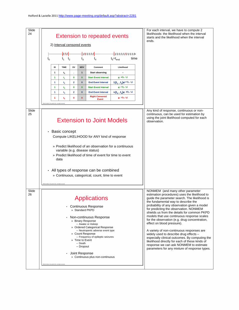
Slide 24
©NHG Holford, M.Lavielle 2011, all rights reserved.
/ / / / / / / / /
Extension to repeated events
t0 time
| x | | x |t1 t2 t3 t4
/ / / / / / / / / / /| x
2) Interval censored events
ID TIME DV MDV Comment Likelihood
1 t0 . 1 Start observing -
1 t1 0 0 Start Event Interval e (t0 , t1)
1 t2 2 0 End Event Interval (t1 , t2)e(t1 , t2)
1 t3 0 0 Start Event Interval e (t2 , t3)
1 t4 2 0 End Event Interval (t3 , t4)e(t3 , t4)
1 t5 0 0Right Censored
Evente (t4 , t5)
t5=tend
For each interval, we have to compute 2 likelihoods: the likelihood when the interval starts and the likelihood when the interval ends.
Slide 25
©NHG Holford, M.Lavielle 2011, all rights reserved.
Extension to Joint Models
• Basic concept
Compute LIKELIHOOD for ANY kind of response
» Predict likelihood of an observation for a continuous
variable (e.g. disease status)
» Predict likelihood of time of event for time to event
data
• All types of response can be combined
» Continuous, categorical, count, time to event
Any kind of response, continuous or non-continuous, can be used for estimation by using the joint likelihood computed for each observation.
Slide 26
©NHG Holford, M.Lavielle 2011, all rights reserved.
Applications
• Continuous Response» Standard PKPD
• Non-continuous Response» Binary Response
– Awake or Asleep
» Ordered Categorical Response– Neutropenic adverse event type
» Count Response– Frequency of epileptic seizures
» Time to Event– Death
– Dropout
• Joint Response» Continuous plus non-continuous
NONMEM (and many other parameter estimation procedures) uses the likelihood to guide the parameter search. The likelihood is the fundamental way to describe the probability of any observation given a model for predicting the observation. NONMEM shields us from the details for common PKPD models that use continuous response scales for the observation (e.g. drug concentration, effect on blood pressure). A variety of non-continuous responses are widely used to describe drug effects – especially clinical outcomes. By computing the likelihood directly for each of these kinds of response we can ask NONMEM to estimate parameters for any mixture of response types.

Holford & Lavielle 2011 http://www.page-meeting.org/default.asp?abstract=2281
Slide 27
©NHG Holford, M.Lavielle 2011, all rights reserved.
Joint Model Data
ID TIME TRT DVID DV MDV Comment
1 0 0 . . 1 Start observing
1 20 0 1 67.4 0 Biomarker
1 30 0 1 43.2 0 Biomarker
1 50 0 2 1 0 Exact Time Event
2 0 1 . . 1 Start observing
2 25 1 1 50.2 0 Biomarker
2 40 1 1 43.7 0 Biomarker
2 60 1 1 13.5 0 Biomarker
2 100 1 2 0 0 Censored Event
The TRT data item indicates if the subject is receiving active treatment (TRT=1) or not (TRT=0). DVID is used to distinguish between continuous value biomarker observations (e.g. DVID=1 for drug concentration) and event observations (e.g. DVID=2).
Slide 28
©NHG Holford, M.Lavielle 2011, all rights reserved.
Example of Joint Model:
Disease Progress and Time Varying Hazard
tbatf )( )()( tfeht
)()()( ttfty
1) Continuous biomarker 2) Time to event
Statistical model:
• IIV on a and b
• Treatment effect on b
Slide 29
©NHG Holford, M.Lavielle 2011, all rights reserved.
Disease Progress and Time Varying Hazard
NONMEM
$INPUT ID TRT DVID TIME DV MDV
$ESTIM MAX=9990 NSIG=3 SIGL=9
METHOD=CONDITIONAL
LAPLACE
$SUBR ADVAN=6 TOL=9
$MODEL
COMP=(CUMHAZ)
$PK
IF (NEWIND.LE.1) CHLAST=0 ; Initialize
;------------------------------
; Hazard
BASHAZ = THETA(1) ; Baseline hazard
BETADP = THETA(2) ; Disease progress effect
;------------------------------
; Symptomatic treatment effect
EFFECT = TRT*THETA(3)
;------------------------------
;Disease Progress
INTRI = (THETA(4)+ EFFECT)*EXP(ETA(1)
SLOPI = THETA(5)* EXP(ETA(2)
$DES
DPRG = INTRI + SLOPI*T
DADT(1) = BASHAZ*EXP(BETADP*DPRG) ; h(t)
$ERROR
CUMHAZ=A(1) ; Cumulative hazard
DISPRG=INTRI + SLOPI*TIME
;------------------------------
IF (DVID.EQ.1) THEN ; disease progress
F_FLAG = 0 ; Continuous
Y = DISPRG + ERR(1); Disease Progress
ENDIF
;------------------------------
IF (DVID.EQ.2.AND.DV.EQ.0) THEN ; right censored
F_FLAG = 1 ; Likelihood
Y = EXP(-CUMHAZ)
CHLAST=CUMHAZ ; start of interval
ELSE
CHLAST=CHLAST ; keep NM-TRAN happy
ENDIF
;------------------------------
IF (DVID.EQ.2.AND.DV.EQ.1) THEN ; exact time
F_FLAG = 1 ; Likelihood
HAZARD = BASHAZ*EXP(BETADP*DISPRG)
Y = EXP(-CUMHAZ)*HAZARD
ENDIF
;------------------------------
IF (DVID.EQ.2.AND.DV.EQ.2) THEN ; interval censored
F_FLAG = 1 ; Likelihood
Y = 1 – EXP(-(CHLAST-CUMHAZ))
ENDIF
This illustrates joint modelling for disease progress and an event. The event hazard depends on disease progress. A differential equation is used to integrate the hazard. An effect of treatment (TRT) is assumed to affect the intercept of the disease progress model which in turn influences the hazard of the event. It is useful to be able to save the value of the cumulative hazard in order to calculate the likelihood of an interval censored event. In this example DV=0 is used to indicate the start of the interval censored event period and the cumulative hazard at this time is saved in the CHLAST variable. The F_FLAG variable is used to tell NONMEM how to use the predicted Y value. F_FLAG of 0 is the default i.e. Y is the prediction of a continuous variable. F_FLAG of 1 means the prediction is a likelihood. F_FLAG of 2 means the prediction is -2*ln(Likelihood).

Holford & Lavielle 2011 http://www.page-meeting.org/default.asp?abstract=2281
Slide 30
©NHG Holford, M.Lavielle 2011, all rights reserved.
Disease Progress and Time Varying Hazard
MONOLIX 4
$DATA ;information in the dataset
ID, TRT use=cov type =cat, TIME, DVID, DV, MDV
$INDIVIDUAL ;distribution of the individual parameters
default dist=log-normal,
INTRI, SLOPI cov=TRT, BASHAZ iiv=no, BETADP iiv=no
$EQUATION
DISPRG= INTRI + SLOPE*T
$EVENT
lambda=BASHAZ*EXP(BETADP*DISPRG)
$OBSERVATIONS distribution of the observations
Biomarker type=continuous pred=DISPRG err=constant,
Death type=event hazard=lambda
Slide 31
©NHG Holford, M.Lavielle 2011, all rights reserved.
Extension to count data
t0
x xx x x x x x x x x xT1 T2T3 T4 T5 T6 T7 T8 T9 T10 T11 T12
The exact times of event
Slide 32
©NHG Holford, M.Lavielle 2011, all rights reserved.
Extension to count data
t0
x xx x x x x x x x x x
t0 t1 t2 t3 t4 t5 t6 t7
x xx x x x x x x x x x| | | | | | | |
T1 T2T3 T4 T5 T6 T7 T8 T9 T10 T11 T12
The exact times of event
are not observed …

Holford & Lavielle 2011 http://www.page-meeting.org/default.asp?abstract=2281
Slide 33
©NHG Holford, M.Lavielle 2011, all rights reserved.
Extension to count data
t0
x xx x x x x x x x x x
t0 t1 t2 t3 t4 t5 t6 t7
x xx x x x x x x x x x| | | | | | | |
T1 T2T3 T4 T5 T6 T7 T8 T9 T10 T11 T12
t0 t1 t2 t3 t4 t5 t6 t7
| | | | | | | |
The exact times of event
are not observed …
Only the number of events in each interval is observed
1 3 2 1 0 2 3
Slide 34
©NHG Holford, M.Lavielle 2011, all rights reserved.
Extension to count data
The count data is a (non homogenous) Poisson process.
The expected number of events in interval [a , b] is
b
a
dttba )(),(
Here, an observation is the number of events in an interval. A careful calculation of the likelihood of this number of observations is not straightforward… but is possible! We can show that this number of observations is a Poisson process. The Poisson parameter in any interval a-b is the expected number of events in this interval: it is defined as the risk (the cumulative hazard) in this interval.
Slide 35
©NHG Holford, M.Lavielle 2011, all rights reserved.
ID TIME DV MDV Likelihood
1 t0 . 1 -
1 t1 1 0 (t0 , t1)e(t0 , t1)
1 t2 3 0 (t1 , t2)3 e (t1 , t2) /3!
1 t3 2 0 (t2 , t3)2 e (t2 , t3) /2!
1 t4 1 0 (t3 , t4)e(t3 , t4)
1 t5 0 0 e (t4 , t5)
1 t6 2 0 (t5 , t6)2 e (t5 , t6) /2!
1 t7 3 0 (t6 , t7)3 e (t6 , t7) /3!
t0 t1 t2 t3 t4 t5 t6 t7
| | | | | | | | 1 3 2 1 0 2 3
Extension to count data
Unlike the previous examples the DV value is used to indicate the number of events in the interval. It does not indicate the event type (exact time, right, interval censored).

Holford & Lavielle 2011 http://www.page-meeting.org/default.asp?abstract=2281
Slide 36
©NHG Holford, M.Lavielle 2011, all rights reserved.
Outcome Event Hazard in Parkinson‟s Disease
deprenyl(t) = 1 for on periods, 0 for
off periods
status(t) = predicted disease status as measured by UPDRS or its subscales at time t
Other Explanatory Factors: (Xn)
•Levodopa(t), baseline motor subtypes status
•Age, sex, smoking status at study entry
Hazard Model with Explanatory Variables
h(t) = h0(t) ·exp( deprenyl·deprenyl(t) + status·status(t) + …+ nXn)
The severity of Parkinson‟s disease is usually assessed by the Unified Parkinson‟s disease response scale (UPDRS). The UPDRS score increases with time as the disease progresses. The disease status can be described by a model for disease progression (natural history) and the effects of treatment e.g. the use of levodopa (the mainstay of treatment) with or without deprenyl (a mono-amine oxidase inhibitor commonly used as an adjunctive treatment) The hazard of a clinical outcome event e.g. death, can be described by a baseline hazard, h0(t), and explanatory factors such as drug treatment and the time course of disease status. Other factors (age, sex, smoking, etc) are easily included in this kind of model.
Slide 37
©NHG Holford, M.Lavielle 2011, all rights reserved.
Evaluation of Hazard Models
visual predictive check
Death Disability
DepressionCognitive Impairment
The change of disease status, reflected by the time course of UPDRS, is the most important factor determining the hazard of clinical outcome events in Parkinson‟s disease. The different shapes of the survival function for death, disability, cognitive impairment and depression reflect different contributions of disease status to the probability of not having had the event as time passes.
Slide 38
©NHG Holford, M.Lavielle 2011, all rights reserved.
Putting Time Back
into The Picture
“Science is either
stamp collecting or physics”Ernest Rutherford
Stamp
CollectingPhysicsModels
Biomarker
+
Time
OutcomeHazard
+
Time

Holford & Lavielle 2011 http://www.page-meeting.org/default.asp?abstract=2281
Slide 39
©NHG Holford, M.Lavielle 2011, all rights reserved.
Backup Slides
Slide 40
©NHG Holford, M.Lavielle 2011, all rights reserved.
Constant hazard (t)
tetTP )(
T is a random variable with an exponential distribution:
0 0.5 1 1.5 2 2.5 3 3.5 4 4.5 5
0
0.1
0.2
0.3
0.4
0.5
0.6
0.7
0.8
0.9
1
time (h)
P(
T >
t )
= 0.5 h-1
= 1 h-1
= 2 h-1
The survival function of a constant hazard decreases exponentially to 0.
Slide 41
©NHG Holford, M.Lavielle 2011, all rights reserved.
Constant hazard (t)
teTtTPaTatTP )0()(
Important property: this distribution is memoryless
0 0.5 1 1.5 2 2.5 3 3.5 4 4.5 5
0
0.2
0.4
0.6
0.8
1
P( T > t ) P( T > t | T > 1) P( T > t | T > 3)
time (h)
Constant hazard makes the very strong assumption of memoryless. The modeller should be aware of this strong assumption at the time to select a hazard function. Consider for example that your event is the first passing of the viral load (HIV, HCV,…) under a given threshold (e.g. LOQ). Here, t_0 is the time when the active treatment starts. We assume that the initial viral load at t_0 is above this threshold. Then : - the hazard is 0 at t_0 and increases with time - if you know that you are still above the threshold after 6 months for instance, then this information will “modify” the distribution of your event time : P(T > t+a | T>a) > P(T>t | T>0) In other words, you are more likely to be a no responder and the probability to reach the threshold decreases This is one of the many examples where a constant hazard is a very poor choice and

Holford & Lavielle 2011 http://www.page-meeting.org/default.asp?abstract=2281
when alternative models (Weibull for instance) should be considered.
Slide 42
©NHG Holford, M.Lavielle 2011, all rights reserved.
Parametric Regression
In Standard Packages
• Estimation of hazard parameters is done after transformation e.g. ln(T)
• Explanatory variable model is then linear regression e.g. for Weibull
ipipiii xxx)(T ...ln 2211
Note that covariates (x1…xp) are usually assumed to be time invariant
Standard survival analysis is equivalent to non-compartmental PK.
It is useful for description but ignores time variation.
ipipiii xxxT ...)ln(1
)ln( 2211
Or more generally
When covariates change with time then the hazard must be integrated in a piecewise fashion. This is exactly analogous to PK problems. If clearance changes from one time period to the next then the concentration prediction must be done piecewise (NONMEM describes this as „advancing the solution‟)
Slide 43
©NHG Holford, M.Lavielle 2011, all rights reserved.
Distribution of Survival Times
Michaelis-Menten Elimination
hazard(t))Survival(tPDF(t)
thazard(t)d
e)Survival(t
b
0-
54.543.532.521.510.50
1
0.9
0.8
0.7
0.6
0.5
0.4
0.3
0.2
0.1
0
2
1.8
1.6
1.4
1.2
1
0.8
0.6
0.4
0.2
0
TIME
su
rviv
al
hazard
, P
DF
survival:1
hazard:1
PDF:1
A useful view of survival is to look at the probability density function for the survival times.

Holford & Lavielle 2011 http://www.page-meeting.org/default.asp?abstract=2281
Slide 44
©NHG Holford, M.Lavielle 2011, all rights reserved.
How can the effect of treatment
Rx(t) be described?
h(t) = f(sex, race, age(t), Rx(t),…)
Rx(t)
Standard survival analysis can include varying age implicitly. Adding time-varying covariates for survival analysis is harder to do because of the need to integrate the hazard. Drug treatments will often change with time and if expressed in terms of drug concentration the hazard could change in proportion to concentration after every dose.
Slide 45
©NHG Holford, M.Lavielle 2011, all rights reserved.
Survivor Function
0
0.1
0.2
0.3
0.4
0.5
0.6
0.7
0.8
0.9
1
0 2 4 6 8 10
Surv
ivo
r Fu
nct
ion
Time (y)
Constant Hazard Time varying hazard
An example of how to simulate the time course of survivor function, cumulative hazard and pdf with a continuously time varying hazard using Berkeley Madonna code. METHOD RK4 STARTTIME = 0 STOPTIME=10 DT = 0.02 beta0=0.1 betaStatus=0.01 S0=20 status=S0+12*time hazpla=beta0*exp(betaStatus*S0) haztrt=beta0*exp(betaStatus*status) init(cumpla)=0 d/dt(cumpla)=hazpla survpla=exp(-cumpla) init(cumtrt)=0 d/dt(cumtrt)=haztrt survtrt=exp(-cumtrt) pdfpla=survpla*hazpla pdftrt=survtrt*haztrt

Holford & Lavielle 2011 http://www.page-meeting.org/default.asp?abstract=2281
Slide 46
©NHG Holford, M.Lavielle 2011, all rights reserved.
Cumulative Hazard and
Relative Risk
0
0.5
1
1.5
2
2.5
0
0.5
1
1.5
2
2.5
0 2 4 6 8 10
Cu
mu
lati
ve H
azar
d
Re
lati
ve R
isk
Time (y)
Relative Risk Constant Hazard
Time varying hazard
Slide 47
©NHG Holford, M.Lavielle 2011, all rights reserved.
Probability Density Function
0
0.05
0.1
0.15
0 2 4 6 8 10
S(t)
* h
(t)
Time (y)
Constant Hazard Time varying hazard
Slide 48
©NHG Holford, M.Lavielle 2011, all rights reserved.
Hazard models link disease progress and
clinical outcome probability
tth
etTtS 0)(
)Pr()(h(t)= 0
h(t)= 0·exp( status·status(t))
Hazard FunctionSurvivor Function
0
0.1
0.2
0.3
0.4
0.5
0 2 4 6 8 10
Haz
ard
(1/y
)
Time (y)
Constant Hazard Time varying hazard
0
0.1
0.2
0.3
0.4
0.5
0.6
0.7
0.8
0.9
1
0 2 4 6 8 10
Surv
ivor
Fun
ctio
n
Time (y)
Constant Hazard Time varying hazard

Holford & Lavielle 2011 http://www.page-meeting.org/default.asp?abstract=2281
Slide 49
©NHG Holford, M.Lavielle 2011, all rights reserved.
Likelihoods for Survival
http://en.wikipedia.org/wiki/Survival_analysis
= S(Ti|θ) * h(Ti)
An alternative way of describing the likelihoods in terms of the survivor function and hazard function alone.